Fast convex optimization via inertial dynamics with Hessian driven damping

Abstract.

We first study the fast minimization properties of the trajectories of the second-order evolution equation

$$\ddot{x}(t)+\frac{\alpha}{t}\dot{x}(t)+\beta\nabla^{2}\Phi(x(t))\dot{x}(t)+\nabla\Phi(x(t))=0,$$

where $\Phi:\mathcal{H}\to\mathbb{R}$ is a smooth convex function acting on a real Hilbert space $\mathcal{H}$, and $\alpha$, $\beta$ are positive parameters. This inertial system combines an isotropic viscous damping which vanishes asymptotically, and a geometrical Hessian driven damping, which makes it naturally related to Newton’s and Levenberg-Marquardt methods. For $\alpha\geq 3$, and $\beta>0$, along any trajectory, fast convergence of the values

$$\Phi(x(t))-\min_{\mathcal{H}}\Phi=\mathcal{O}\left(t^{-2}\right)$$

is obtained, together with rapid convergence of the gradients $\nabla\Phi(x(t))$ to zero. For $\alpha>3$, just assuming that ${\rm argmin}\kern 1.19995pt\Phi\neq\emptyset,$ we show that any trajectory converges weakly to a minimizer of $\Phi$, and that $\Phi(x(t))-\min_{\mathcal{H}}\Phi=o(t^{-2})$. Strong convergence is established in various practical situations. In particular, for the strongly convex case, we obtain an even faster speed of convergence which can be arbitrarily fast depending on the choice of $\alpha$. More precisely, we have $\Phi(x(t))-\min_{\mathcal{H}}\Phi=\mathcal{O}(t^{-\frac{2}{3}\alpha})$. Then, we extend the results to the case of a general proper lower-semicontinuous convex function $\Phi:\mathcal{H}\rightarrow\mathbb{R}\cup\{+\infty\}$. This is based on the crucial property that the inertial dynamic with Hessian driven damping can be equivalently written as a first-order system in time and space, allowing to extend it by simply replacing the gradient with the subdifferential. By explicit-implicit time discretization, this opens a gate to new $-$ possibly more rapid $-$ inertial algorithms, expanding the field of FISTA methods for convex structured optimization problems.

Introduction

Throughout the paper, $\mathcal{H}$ is a real Hilbert space endowed with scalar product $\langle\cdot,\cdot\rangle$ and norm $\|x\|=\sqrt{\langle x,x\rangle}$ for $x\in\mathcal{H}$. Let $\Phi:\mathcal{H}\rightarrow\mathbb{R}$ be a twice continuously differentiable convex function (the case of a nonsmooth function will be considered later on). In view of the minimization of $\Phi$, we study the asymptotic behaviour (as $t\to+\infty$) of the trajectories of the second-order differential equation

(1) $$\boxed{\mbox{(DIN-AVD)}\quad\quad\ddot{x}(t)+\frac{\alpha}{t}\dot{x}(t)+\beta\nabla^{2}\Phi(x(t))\dot{x}(t)+\nabla\Phi(x(t))=0}$$

where $\alpha$ and $\beta$ are positive parameters.

This inertial system combines two types of damping:

In the first place, the term $\frac{\alpha}{t}\dot{x}(t)$ furnishes an isotropic linear damping with a viscous parameter $\frac{\alpha}{t}$ which vanishes asymptotically, but not too slowly. The asymptotic behavior of the inertial gradient-like system

(2) $$\mbox{(AVD)}\quad\quad\ddot{x}(t)+a(t)\dot{x}(t)+\nabla\Phi(x(t))=0,$$

with Asymptotic Vanishing Damping ((AVD) for short), has been studied by Cabot, Engler and Gaddat in [21]-[22]. They proved that, under moderate decrease of $a$ to zero, namely, that $\lim_{t\to+\infty}a(t)=0$ and $\int_{0}^{\infty}a(t)dt=+\infty$, every solution $x$ of (2) satisfies $\lim_{t\to+\infty}\Phi(x(t))\to\min_{\mathcal{H}}\Phi$.

Interestingly, with the specific choice $a(t)=\frac{\alpha}{t}$:

(3) $$\ddot{x}(t)+\frac{\alpha}{t}\dot{x}(t)+\nabla\Phi(x(t))=0,$$

Su, Boyd and Candès in [36] proved the fast convergence property

(4) $$\Phi(x(t))-\min_{\mathcal{H}}\Phi=\mathcal{O}\left(t^{-2}\right),$$

provided $\alpha\geq 3$. In the same article, the authors show that, for $\alpha=3$, (3) can be seen as a continuous-time version of the fast convergent method of Nesterov [29]-[30]-[31]-[32]. In [13], Attouch, Peypouquet and Redont showed that, for $\alpha>3$, each trajectory of (3) converges weakly to an element of ${\rm argmin}\kern 1.19995pt\Phi$. This result is a continuous-time counterpart to the Chambolle-Dossal algorithm [23], which is a modified Nesterov algorithm specially designed to obtain the convergence of the iterates.

In the second place, a geometrical damping, attached to the term $\beta\nabla^{2}\Phi(x(t))\dot{x}(t)$, has a natural link with Newton’s method. It gives rise to the so-called Dynamical Inertial Newton system ((DIN) for short)

(5) $$\mbox{(DIN)}\quad\quad\ddot{x}(t)+\gamma\dot{x}(t)+\beta\nabla^{2}\Phi(x(t))\dot{x}(t)+\nabla\Phi(x(t))=0,$$

which has been introduced by Alvarez, Attouch, Bolte and Redont in [6] ($\gamma$ is a fixed positive parameter). Interestingly, (5) can be equivalently written as a first-order system involving only the gradient of $\Phi$, which allows its extension to the case of a proper lower-semicontinuous convex function $\Phi$. This led to applications ranging from optimization algorithms [12] to unilateral mechanics and partial differential equations [11].

As we shall see, (DIN-AVD) inherits the convergence properties of both (AVD) and (DIN), but exhibits other important features, namely (see Theorems 1.10, 1.14, 1.15, 3.1, 4.8, 4.11, 4.12):

• Assuming $\alpha\geq 3$, $\beta>0$ and ${\rm argmin}\kern 1.19995pt\Phi\neq\emptyset$, we show the fast convergence property of the values (4), together with the fast convergence to zero of the gradients

  (6) $$\int_{0}^{\infty}t^{2}\|\nabla\Phi(x(t))\|^{2}dt<+\infty.$$

• For $\alpha>3$, we complete these results by showing that every trajectory converges weakly, with its limit belonging to ${\rm argmin}\kern 1.19995pt\Phi$. Moreover, we obtain a faster order of convergence $\Phi(x(t))-\min_{\mathcal{H}}\Phi=o(t^{-2})$.

• Also for $\alpha>3$, strong convergence is established in various practical situations. In particular, for the strongly convex case, we obtain an even faster speed of convergence which can be arbitrarily fast according to the choice of $\alpha$. More precisely, we have $\Phi(x(t))-\min_{\mathcal{H}}\Phi=\mathcal{O}(t^{-\frac{2}{3}\alpha})$.

• A remarkable property of the system (DIN-AVD) is that these results can be naturally generalized to the non-smooth convex case. The key argument is that it can be reformulated as a first-order system (both in time and space) involving only the gradient and not the Hessian!

Time discretization of (DIN-AVD) provides new ideas for the design of innovative fast converging algorithms, expanding the field of rapid methods for structured convex minimization of Nesterov [29, 30, 31, 32], Beck-Teboulle [16], and Chambolle-Dossal [23]. This study, however, goes beyond the scope of this paper, and will be carried out in a future research. As briefly evoked above, the continuous (DIN-AVD) system is also linked to the modeling of non-elastic shocks in unilateral mechanics, and the geometric damping of nonlinear oscillators. These are important areas for applications, which are not considered in this paper.

1. Smooth potential

The following minimal hypotheses are in force in this section, and are always tacitly assumed:

• $\alpha>0$, $\beta>0$;

• $\Phi:\mathcal{H}\rightarrow\mathbb{R}$ is a twice continuously differentiable convex function; and

• $t_{0}>0$, $x_{0}\in\mathcal{H}$, $\dot{x}_{0}\in\mathcal{H}$.

In view of minimizing $\Phi$, we study the asymptotic behaviour, as $t\to+\infty$, of a solution $x$ to (DIN-AVD) second-order evolution equation (1). We will successively examine the following points:

• existence and uniqueness of a solution $x$ to (DIN-AVD) with Cauchy data $x(t_{0})=x_{0}$ and $\dot{x}(t_{0})=\dot{x}_{0}$;

• minimizing properties of $x$ and convergence of $\Phi(x(t))$ towards $\inf\Phi$ whenever $\alpha>0$;

• fast convergence of $\Phi(x(t))$ towards $\min\Phi$, when the latter is attained and $\alpha\geq 3$;

• weak convergence of $x$ towards a minimum of $\Phi$ and faster convergence of $\Phi(x(t))$, when $\alpha>3$;

• some cases of strong convergence of $x$, and faster convergence of $\Phi(x(t))$.

1.1. Existence and uniqueness of solution

The following result will be derived in Section 4 from a more general result concerning a convex lower semicontinuous function $\Phi:\mathcal{H}\rightarrow{\mathbb{R}}\cup\{+\infty\}$ (see Corollary 4.6 below):

Theorem 1.1.

For any Cauchy data $(x_{0},\dot{x}_{0})\in\mathcal{H}\times\mathcal{H}$, (DIN-AVD) admits a unique twice continuously differentiable global solution $x:[t_{0},+\infty[\rightarrow\mathcal{H}$ verifying $(x(t_{0}),\dot{x}(t_{0}))=(x_{0},\dot{x}_{0})$.

1.2. Lyapunov analysis and minimizing properties of the solutions for $\alpha>0$

In this section, we present a family of Lyapunov functions for (DIN-AVD), and use them to derive the main properties of the solutions to this system. As we shall see, the fact that we have more than one (essentially different) of these functions will play a crucial role in establishing that the gradient vanishes as $t\to+\infty$.

Let $x:t\in[t_{0},\infty[\to\mathcal{H}$ satisfy (DIN-AVD) with Cauchy data $x(t_{0})=x_{0}$ and $\dot{x}(t_{0})=\dot{x}_{0}$, and let $\theta\in[0,\beta]$. Define $W_{\theta}:[t_{0},+\infty[\to{\mathbb{R}}$ by

(7) $$W_{\theta}(t)=\Phi(x(t))+\frac{1}{2}\|\dot{x}(t)+\theta\nabla\Phi(x(t))\|^{2}+\frac{\theta(\beta-\theta)}{2}\|\nabla\Phi(x(t))\|^{2}.$$

Observe that, for $\theta=0$, we obtain

$$W_{0}(t)=\Phi(x(t))+\frac{1}{2}\|\dot{x}(t)\|^{2},$$

which is the usual global mechanical energy of the system. We shall see that, for each $\theta\in[0,\beta]$, $W_{\theta}$ is a strict Lyapunov function for (DIN-AVD).

In order to simplify the notation, write

(8) $$u_{\theta}(t)=x(t)+\theta\int_{t_{0}}^{t}\nabla\Phi(x(s))ds,$$

so that  $u_{0}(t)=x(t),$ and, for each $\theta\in[0,\beta]$,

(9) $$\dot{u}_{\theta}(t) = \dot{x}(t)+\theta\nabla\Phi(x(t))$$

$$W_{\theta}(t) = \Phi(x(t))+\frac{1}{2}\|\dot{u}_{\theta}(t)\|^{2}+\frac{\theta(\beta-\theta)}{2}\|\nabla\Phi(x(t))\|^{2}.$$

Using (9) and (DIN-AVD), elementary computations yield

(10) $$\ddot{u}_{\theta}(t)=\ddot{x}(t)+\theta\nabla^{2}\Phi(x(t))\dot{x}(t)=-\frac{\alpha}{t}\dot{x}(t)-\nabla\Phi(x(t))+(\theta-\beta)\nabla^{2}\Phi(x(t))\dot{x}(t).$$

We have the following:

Proposition 1.2.

Let $\alpha>0$, and suppose $x:[t_{0},+\infty[\rightarrow\mathcal{H}$ is a solution of (DIN-AVD). Then, for each $\theta\in[0,\beta]$ and $t\geq\max\{t_{0},\frac{\alpha\theta}{2}\}$, we have

$$\dot{W}_{\theta}(t)\leq-\frac{\alpha}{2t}\|\dot{x}(t)\|^{2}-\frac{\alpha}{2t}\|\dot{u}_{\theta}(t)\|^{2}.$$

Proof.

First observe that

(11) $$\dot{W}_{\theta}(t)=\langle\nabla\Phi(x(t)),\dot{x}(t)\rangle+\langle\ddot{u}_{\theta}(t),\dot{u}_{\theta}(t)\rangle+\theta(\beta-\theta)\langle\nabla^{2}\Phi(x(t))\dot{x}(t),\nabla\Phi(x(t))\rangle.$$

Next, use (9) and (10) to obtain

$$\langle\ddot{u}_{\theta}(t),\dot{u}_{\theta}(t)\rangle = \langle-\frac{\alpha}{t}\dot{x}(t)-\nabla\Phi(x(t))+(\theta-\beta)\nabla^{2}\Phi(x(t))\dot{x}(t),\dot{x}(t)+\theta\nabla\Phi(x(t))\rangle$$

$$= -\frac{\alpha}{t}\|\dot{x}(t)\|^{2}-(\frac{\alpha\theta}{t}+1)\langle\nabla\Phi(x(t)),\dot{x}(t)\rangle-\theta\|\nabla\Phi(x(t))\|^{2}+(\theta-\beta)\langle\nabla^{2}\Phi(x(t))\dot{x}(t),\dot{x}(t)\rangle$$

$$\quad+\theta(\theta-\beta)\langle\nabla^{2}\Phi(x(t))\dot{x}(t),\nabla\Phi(x(t))\rangle$$

$$\leq -\frac{\alpha}{t}\|\dot{x}(t)\|^{2}-(\frac{\alpha\theta}{t}+1)\langle\nabla\Phi(x(t)),\dot{x}(t)\rangle-\theta\|\nabla\Phi(x(t))\|^{2}+\theta(\theta-\beta)\langle\nabla^{2}\Phi(x(t))\dot{x}(t),\nabla\Phi(x(t))\rangle,$$

since $\langle\nabla^{2}\Phi(x(t))\dot{x}(t),\dot{x}(t)\rangle\geq 0$ by convexity. From (11), we obtain

(12) $$\dot{W}_{\theta}(t)\leq-\frac{\alpha}{t}\|\dot{x}(t)\|^{2}-\frac{\alpha\theta}{t}\langle\nabla\Phi(x(t)),\dot{x}(t)\rangle-\theta\|\nabla\Phi(x(t))\|^{2}.$$

On the one hand, when $\theta=0$, it immediately follows that

$$\dot{W}_{0}(t)\leq-\frac{\alpha}{t}\|\dot{x}(t)\|^{2}.$$

On the other hand, if $\theta\in]0,\beta]$, we use (9) in (12) to deduce that

$$\dot{W}_{\theta}(t)\leq\left(\frac{2}{\theta}-\frac{\alpha}{t}\right)\langle\dot{u}_{\theta}(t),\dot{x}(t)\rangle-\frac{1}{\theta}\|\dot{x}(t)\|^{2}-\frac{1}{\theta}\|\dot{u}_{\theta}(t)\|^{2}\leq-\frac{\alpha}{2t}\|\dot{x}(t)\|^{2}-\frac{\alpha}{2t}\|\dot{u}_{\theta}(t)\|^{2},$$

since $\frac{2}{\theta}-\frac{\alpha}{t}\geq 0$ by hypothesis, and the fact that $|\langle\zeta,\xi\rangle|\leq\frac{1}{2}\|\zeta\|^{2}+\frac{1}{2}\|\xi\|^{2}$ for all $\zeta,\xi\in\mathcal{H}$. ∎

Theorem 1.3.

Let $\alpha>0$, and suppose $x:[t_{0},+\infty[\rightarrow\mathcal{H}$ is a solution of (DIN-AVD). Then

$$\lim_{t\to+\infty}W_{0}(t)=\lim_{t\to+\infty}W_{\beta}(t)=\lim_{t\to+\infty}\Phi(x(t))=\inf\Phi\in{\mathbb{R}}\cup\{-\infty\}.$$

Proof.

Since we are interested in asymptotic properties of $x$, we can assume $t\geq t_{1}=\max\{t_{0},\alpha\beta\}$ throughout the proof. Take $\theta\in\{0,\beta\}$, so that the last term in the definition (7) of $W_{\theta}$ vanishes. Given $z\in\mathcal{H}$, we define $h:[t_{1},+\infty[\to{\mathbb{R}}$ by

$$h(t)=\frac{1}{2}\|u_{\theta}(t)-z\|^{2}.$$

By the Chain Rule, we have

$$\dot{h}(t)=\langle u_{\theta}(t)-z,\dot{u}_{\theta}(t)\rangle\qquad\hbox{and}\qquad\ddot{h}(t)=\langle u_{\theta}(t)-z,\ddot{u}_{\theta}(t)\rangle+\|\dot{u}_{\theta}(t)\|^{2}.$$

On the other hand, from (9) and (10), we obtain

(13) $$\ddot{u}_{\theta}(t)+\frac{\alpha}{t}\dot{u}_{\theta}(t)=\left(\frac{\alpha\theta}{t}-1\right)\nabla\Phi(x(t))+(\theta-\beta)\nabla^{2}\Phi(x(t))\dot{x}(t).$$

Set

$$I(t):=\frac{1}{2}\left\|\int_{t_{0}}^{t}\nabla\Phi(x(s))ds\right\|^{2}\qquad\hbox{and}\qquad J(t):=\langle x(t)-z,\nabla\Phi(x(t))\rangle-\Phi(x(t)),$$

and observe that

$$\dot{I}(t)=\left\langle\int_{t_{0}}^{t}\nabla\Phi(x(s))ds,\nabla\Phi(x(t))\right\rangle\qquad\hbox{and}\qquad\dot{J}(t)=\langle x(t)-z,\nabla^{2}\Phi(x(t))\dot{x}(t)\rangle.$$

Next, since $\theta\in\{0,\beta\}$, we can write

$$\ddot{h}(t)+\frac{\alpha}{t}\dot{h}(t) = \|\dot{u}_{\theta}(t)\|^{2}+\left(\frac{\alpha\theta}{t}-1\right)\langle u_{\theta}(t)-z,\nabla\Phi(x(t))\rangle+(\theta-\beta)\langle u_{\theta}(t)-z,\nabla^{2}\Phi(x(t))\dot{x}(t)\rangle$$

$$= \|\dot{u}_{\theta}(t)\|^{2}+\left(\frac{\alpha\theta}{t}-1\right)\langle x(t)-z,\nabla\Phi(x(t))\rangle+\theta\left(\frac{\alpha\theta}{t}-1\right)\dot{I}(t)+(\theta-\beta)\dot{J}(t)$$

$$\leq \|\dot{u}_{\theta}(t)\|^{2}+\left(\frac{\alpha\theta}{t}-1\right)\big{(}\Phi(x(t))-\Phi(z)\big{)}+\theta\left(\frac{\alpha\theta}{t}-1\right)\dot{I}(t)+(\theta-\beta)\dot{J}(t),$$

where the last inequality follows from the convexity of $\Phi$ and the fact that $t\geq\alpha\beta\geq\alpha\theta$. Using the definition (7) of $W_{\theta}$, and Proposition 1.2, we get

$$\ddot{h}(t)+\frac{\alpha}{t}\dot{h}(t) = \left(\frac{3}{2}-\frac{\alpha\theta}{2t}\right)\|\dot{u}_{\theta}(t)\|^{2}+\left(\frac{\alpha\theta}{t}-1\right)\big{(}W_{\theta}(t)-\Phi(z)\big{)}+\theta\left(\frac{\alpha\theta}{t}-1\right)\dot{I}(t)+(\theta-\beta)\dot{J}(t)$$

$$\leq -\left(\frac{3t}{\alpha}-\theta\right)\dot{W}_{\theta}(t)+\left(\frac{\alpha\theta}{t}-1\right)\big{(}W_{\theta}(t)-\Phi(z)\big{)}+\theta\left(\frac{\alpha\theta}{t}-1\right)\dot{I}(t)+(\theta-\beta)\dot{J}(t).$$

Dividing by $t$ and rearranging the terms, we have

$$\frac{1}{t}\ddot{h}(t)+\left(\frac{1}{t}-\frac{\alpha\theta}{t^{2}}\right)\big{(}W_{\theta}(t)-\Phi(z)\big{)}\leq-\left(\frac{3}{\alpha}-\frac{\theta}{t}\right)\dot{W}_{\theta}(t)-\left[\frac{\alpha}{t^{2}}\dot{h}(t)+\theta\left(\frac{1}{t}-\frac{\alpha\theta}{t^{2}}\right)\dot{I}(t)+\frac{(\beta-\theta)}{t}\dot{J}(t)\right].$$

Since $h$, $I$ and $J$ are bounded from below, we can integrate this inequality from $t_{1}$ to $t$, and use Lemma 7.3 to obtain $C\in{\mathbb{R}}$ such that

(14) $$\frac{1}{t}\dot{h}(t)+\int_{t_{1}}^{t}\left(\frac{1}{s}-\frac{\alpha\theta}{s^{2}}\right)\big{(}W_{\theta}(s)-\Phi(z)\big{)}\,ds\leq-\int_{t_{1}}^{t}\left(\frac{3}{\alpha}-\frac{\theta}{s}\right)\dot{W}_{\theta}(s)\,ds+C.$$

Since $W_{\theta}$ is nonincreasing, we have

(15) $$\int_{t_{1}}^{t}\left(\frac{1}{s}-\frac{\alpha\theta}{s^{2}}\right)\big{(}W_{\theta}(s)-\Phi(z)\big{)}\,ds \geq \big{(}W_{\theta}(t)-\Phi(z)\big{)}\int_{t_{1}}^{t}\left(\frac{1}{s}-\frac{\alpha\theta}{s^{2}}\right)\,ds$$

$$= \big{(}W_{\theta}(t)-\Phi(z)\big{)}\left(\ln t-\ln t_{1}+\frac{\alpha\theta}{t}-\frac{\alpha\theta}{t_{1}}\right).$$

In turn,

(16) $$-\int_{t_{1}}^{t}\left(\frac{3}{\alpha}-\frac{\theta}{s}\right)\dot{W}_{\theta}(s)\,ds = \left(\frac{3}{\alpha}-\frac{\theta}{t_{1}}\right)\big{(}W_{\theta}(t_{1})-\Phi(z)\big{)}-\left(\frac{3}{\alpha}-\frac{\theta}{t}\right)\big{(}W_{\theta}(t)-\Phi(z)\big{)}+\theta\int_{t_{1}}^{t}\frac{W_{\theta}(s)-\Phi(z)}{s^{2}}\,ds$$

$$\leq \left(\frac{3}{\alpha}-\frac{\theta}{t_{1}}\right)\big{(}W_{\theta}(t_{1})-\Phi(z)\big{)}-\left(\frac{3}{\alpha}-\frac{\theta}{t}\right)\big{(}W_{\theta}(t)-\Phi(z)\big{)}+\theta\big{(}W_{\theta}(t_{1})-\Phi(z)\big{)}\left(\frac{1}{t_{1}}-\frac{1}{t}\right),$$

$$\leq \frac{3}{\alpha}\big{|}W_{\theta}(t_{1})-\Phi(z)\big{|}-\left(\frac{3}{\alpha}-\frac{\theta}{t}\right)\big{(}W_{\theta}(t)-\Phi(z)\big{)},$$

since $t\mapsto W_{\theta}(t)-\Phi(z)$ is nonincreasing and $t\geq t_{1}\geq\alpha\beta\geq\alpha\theta$.

Combining (14), (15) and (16), we deduce that

$$\frac{1}{t}\dot{h}(t)+\big{(}W_{\theta}(t)-\Phi(z)\big{)}\left(\ln t+D+\frac{E}{t}\right)\leq C^{\prime}$$

for appropriate constants $C^{\prime},D,E\in{\mathbb{R}}$.

Now, take $t_{2}\geq t_{1}$ such that $\ln s+D+\frac{E}{s}\geq 0$ for all $s\geq t_{2}$, and integrate from $t_{2}$ to $t$ to obtain

$$\frac{h(t)}{t}-\frac{h(t_{2})}{t_{2}}+\int_{t_{2}}^{t}\frac{h(s)}{s^{2}}ds+\big{(}W_{\theta}(t)-\Phi(z)\big{)}\int_{t_{2}}^{t}\left(\log s+D+\frac{E}{s}\right)ds\leq C^{\prime}(t-t_{2}).$$

Since $h$ is nonnegative, this implies

$$-\frac{h(t_{2})}{t_{2}}+\big{(}W_{\theta}(t)-\Phi(z)\big{)}\left(t\ln t-t_{2}\ln t_{2}+(D-1)(t-t_{2})+E(\ln t-\ln t_{2})\right)ds\leq C^{\prime}(t-t_{2}),$$

and so,

(17) $$\big{(}W_{\theta}(t)-\Phi(z)\big{)}\left(t\ln t+(D-1)t+E\ln t+F\right)ds\leq C^{\prime}t+G,$$

for some other constants $F,G\in{\mathbb{R}}$. As $t\to+\infty$, we obtain $\lim_{t\to+\infty}W_{\theta}(t)\leq\Phi(z)$ (the limit is in ${\mathbb{R}}\cup\{-\infty\}$). Since $z$ is arbitrary, and $\inf\Phi\leq\Phi(x(t))\leq W_{\theta}(t)$ for all $t$, the result follows. ∎

By the weak lower-semicontinuity of $\Phi$, Theorem 1.3 immediately yields the following:

Corollary 1.4.

Let $\alpha>0$, and suppose $x:[t_{0},+\infty[\rightarrow\mathcal{H}$ is a solution of (DIN-AVD). As $t\to+\infty$, every sequential weak cluster point of $x(t)$ belongs to ${\rm argmin}\kern 1.19995pt\Phi$. In particular, if $\|x(t)\|$ does not tend to $+\infty$ as $t\to+\infty$, then ${\rm argmin}\kern 1.19995pt\Phi\neq\emptyset$.

If the function $\Phi$ is bounded from below, we have the following stability result:

Proposition 1.5.

Let $\alpha>0$, and suppose $x:[t_{0},+\infty[\rightarrow\mathcal{H}$ is a solution of (DIN-AVD). If $\inf\Phi>-\infty$, then

$$\lim_{t\to+\infty}\|\dot{x}(t)\|=\lim_{t\to+\infty}\|\nabla\Phi(x(t))\|=0,\quad\int_{t_{0}}^{\infty}\frac{1}{t}\|\dot{x}(t)\|^{2}dt<+\infty,\quad\hbox{and}\quad\int_{t_{0}}^{\infty}\frac{1}{t}\|\nabla\Phi(x(t))\|^{2}dt<+\infty.$$

Proof.

Theorem 1.3 establishes that $\lim_{t\rightarrow+\infty}W_{0}(t)=\lim_{t\rightarrow+\infty}W_{\beta}(t)=\lim_{t\rightarrow+\infty}\Phi(x(t))=\inf\Phi\in{\mathbb{R}}\cup\{-\infty\}$. If $\Phi$ is bounded below, the limits belong to ${\mathbb{R}}$. We deduce that

$$\left\{\begin{array}[]{rcccl}\lim\limits_{t\to+\infty}\|\dot{x}(t)\|^{2}&=&2\lim\limits_{t\to+\infty}\big{(}W_{0}(t)-\Phi(x(t))\big{)}&=&0\vskip 6.0pt plus 2.0pt minus 2.0pt\\ \lim\limits_{t\to+\infty}\|\dot{u}_{\beta}(t)\|^{2}&=&2\lim\limits_{t\to+\infty}\big{(}W_{\beta}(t)-\Phi(x(t))\big{)}&=&0.\end{array}\right.$$

By definition (8), we have $\beta\nabla\Phi(x(t))=\dot{u}_{\beta}(t)-\dot{x}(t)$, and so, $\lim_{t\to+\infty}\|\nabla\Phi(x(t))\|=0$. Finally, Proposition 1.2 gives

$$\int_{t_{1}}^{\infty}\frac{\alpha}{2s}(\|\dot{x}(s)\|^{2}+\|\dot{u}_{\beta}(s)\|^{2})\,ds\leq W_{\beta}(t_{1})-\inf\Phi<+\infty.$$

It suffices to use $\beta\nabla\Phi(x(t))=\dot{u}_{\beta}(t)-\dot{x}(t)$ again to complete the proof. ∎

Proposition 1.6.

Let $\alpha>0$, and suppose $x:[t_{0},+\infty[\rightarrow\mathcal{H}$ is a solution of (DIN-AVD). If ${\rm argmin}\kern 1.19995pt\Phi\neq\emptyset$, then

• $\Phi(x(t))-\min\Phi=\mathcal{O}\left(\frac{1}{\log t}\right)$, $\|\dot{x}(t)\|=\mathcal{O}\left(\frac{1}{\sqrt{\log t}}\right)$ and $\|\nabla\Phi(x(t))\|=\mathcal{O}\left(\frac{1}{\sqrt{\log t}}\right)$;

• $\int_{t_{0}}^{\infty}\frac{1}{t}(\Phi(x(t))-\min\Phi)dt<+\infty$.

Proof.

Fix $\hat{z}\in{\rm argmin}\kern 1.19995pt\Phi$.

For i), observe that $0\leq\Phi(x(t))-\min\Phi+\frac{1}{2}\|\dot{u}_{\theta}(t)\|^{2}=W_{\theta}(t)-\min\Phi$. Next, use (17) with $z=\hat{z}$ to conclude.

For ii), use $z=\hat{z}$ in inequalities (14) and (16), and combine them to deduce that

(18) $$\frac{1}{2t}\frac{d}{dt}\|x(t)-\hat{z}\|^{2}+\left(1-\frac{\alpha\theta}{t_{1}}\right)\int_{t_{1}}^{t}\frac{W_{0}(s)-\Phi(z)}{s}\,ds\leq C^{\prime\prime}$$

for $t\geq t_{1}$ and some other constant $C^{\prime\prime}$. On the other hand, since $\lim_{t\to+\infty}\|\dot{x}(t)\|=0$ by Proposition 1.5, we have $\|\dot{x}\|_{\infty}:=\sup_{t\geq t_{0}}\|\dot{x}(t)\|<+\infty$. It follows that

$$\frac{1}{t}\frac{d}{dt}\|x(t)-\hat{z}\|^{2}\leq\frac{1}{t}\|\dot{x}\|_{\infty}\,\|x(t)-\hat{z}\|\leq\|\dot{x}\|_{\infty}\,\left(\frac{\|x(t_{1})-\hat{z}\|}{t_{1}}+\|\dot{x}\|_{\infty}\right)$$

by the Mean Value Theorem. From (18), we deduce that

$$\int_{t_{1}}^{t}\frac{W_{0}(s)-\Phi(z)}{s}\,ds<+\infty$$

which yields the result. ∎

Remark 1.7.

Most of the results in this section can be established without using the differentiability of $\dot{x}$ and $\nabla\Phi(x)$ independently, but only that of $\dot{u}_{\theta}=\dot{x}+\theta\nabla\Phi(x)$, along with relations (9) and (10), and the chain rule $\frac{d}{dt}\Phi(x(t))=\langle\nabla\Phi(x(t)),\dot{x}(t)\rangle$. We shall develop these arguments in Section 4, when we deal with a nonsmooth potential.

1.3. Fast convergence of the values for $\alpha\geq 3$

In this part we mainly analyze the fast convergence of the values of $\Phi$ along a trajectory of (DIN-AVD). The value $\alpha=3$ plays a special role: to our knowledge, it is the smallest for which fast convergence results are proved to hold.

Suppose $\alpha\geq 3$ and $x^{\ast}\in{\rm argmin}\kern 1.19995pt\Phi$. Let $x$ be a solution of (DIN-AVD) with Cauchy data $(x(t_{0}),\dot{x}(t_{0}))=(x_{0},\dot{x}_{0})\in\mathcal{H}\times\mathcal{H}$. For $\lambda\in[2,\alpha-1]$ we define the function $\mathcal{E}_{\lambda}:[t_{0},+\infty[\rightarrow{\mathbb{R}}$ by

(19) $$\mathcal{E}_{\lambda}(t)=t(t-\beta(\lambda+2-\alpha))(\Phi(x(t))-\min\Phi)+\frac{1}{2}\|\lambda(x(t)-x^{\ast})+t\dot{u}_{\beta}(t)\|^{2}+\lambda(\alpha-\lambda-1)\frac{1}{2}\|x(t)-x^{\ast}\|^{2},$$

where $u_{\beta}$ is given by (8), with $\theta=\beta$. To compute $\frac{d}{dt}\mathcal{E}_{\lambda}(t)$ we first differentiate each term of $\mathcal{E}_{\lambda}$ in turn (we use (10) in the second derivative).

$$\frac{d}{dt}[t(t-\beta(\lambda+2-\alpha))(\Phi(x(t))-\min\Phi)]=(2t-\beta(\lambda+2-\alpha))(\Phi(x(t))-\min\Phi)+t(t-\beta(\lambda+2-\alpha))\langle\dot{x}(t),\nabla\Phi(x(t))\rangle;$$

$$\frac{d}{dt}\frac{1}{2}\|\lambda(x(t)-x^{\ast})+t\dot{u}_{\beta}(t)\|^{2} = \langle\lambda(x(t)-x^{\ast})+t\dot{u}_{\beta}(t),\lambda\dot{x}(t)+\dot{u}_{\beta}(t)+t\ddot{u}_{\beta}(t)\rangle$$

$$= \langle\lambda(x(t)-x^{\ast})+t\dot{u}_{\beta}(t),(\lambda+1-\alpha)\dot{x}(t)-(t-\beta)\nabla\Phi(x(t))\rangle$$

$$= \lambda(\lambda+1-\alpha)\langle x(t)-x^{\ast},\dot{x}(t)\rangle-t(\alpha-\lambda-1)\|\dot{x}(t)\|^{2}-\beta t(t-\beta)\|\nabla\Phi(x(t))\|^{2}$$

$$-\lambda(t-\beta)\langle x(t)-x^{\ast},\nabla\Phi(x(t))\rangle-t(t-\beta(\lambda+2-\alpha))\langle\dot{x}(t),\nabla\Phi(x(t))\rangle;$$

$$\frac{d}{dt}\lambda(\alpha-\lambda-1)\frac{1}{2}\|x(t)-x^{\ast}\|^{2} = \lambda(\alpha-\lambda-1)\langle x(t)-x^{\ast},\dot{x}(t)\rangle.$$

Whence

$$\frac{d}{dt}\mathcal{E}_{\lambda}(t) = (2t-\beta(\lambda+2-\alpha))(\Phi(x(t))-\min\Phi)-\lambda(t-\beta)\langle x(t)-x^{\ast},\nabla\Phi(x(t))\rangle$$

$$-t(\alpha-\lambda-1)\|\dot{x}(t)\|^{2}-\beta t(t-\beta)\|\nabla\Phi(x(t))\|^{2}.$$

Now, $\langle x(t)-x^{\ast},\nabla\Phi(x(t))\rangle\geq\Phi(x(t)-\Phi(x^{\ast})$. If $t\geq\max\{t_{0},\beta\}$, we deduce, from (1.3), that

(21) $$\frac{d}{dt}\mathcal{E}_{\lambda}(t)\leq-((\lambda-2)t-\beta(\alpha-2))(\Phi(x(t))-\min\Phi)-t(\alpha-\lambda-1)\|\dot{x}(t)\|^{2}-\beta t(t-\beta)\|\nabla\Phi(x(t))\|^{2}.$$

Remark 1.8.

Recall that $\mathcal{E}_{\lambda}$ is nonnegative. Let us give a closer look at the coefficients on the right-hand side: First, $(\lambda-2)t-\beta(\alpha-2)\geq 0$ for $t\geq t_{1}=\max\{t_{0},\beta,\frac{\beta(\alpha-2)}{\lambda-2}\}$ provided $\lambda>2$. Next, $\alpha-\lambda-1\geq 0$ whenever $\lambda\leq\alpha-1$. A compatibility condition for these two relations to hold is that $2<\lambda\leq\alpha-1$, thus $\alpha>3$. The limiting case $\lambda=2$ (thus $\alpha=3$) will be included in Lemma 1.9 below. Finally, $\beta t(t-\beta)\geq 0$ for $t\geq\beta$. Summarizing, if $\lambda\in]2,\alpha-1]$, we immediately deduce that $\mathcal{E}_{\lambda}$ is nonincreasing on the interval $[t_{1},+\infty[$, and $\lim_{t\rightarrow+\infty}\mathcal{E}_{\lambda}(t)$ exists.

Lemma 1.9.

Let $\alpha\geq 3$ and ${\rm argmin}\kern 1.19995pt\Phi\neq\emptyset$. Suppose $x:[t_{0},+\infty[\rightarrow\mathcal{H}$ is a solution of (DIN-AVD). If $\lambda\in[2,\alpha-1]$, then the function

$$t\mapsto\left(\frac{t}{t-\beta}\right)^{\alpha-2}\mathcal{E}_{\lambda}(t)$$

is nonincreasing and $\lim_{t\rightarrow+\infty}\mathcal{E}_{\lambda}(t)$ exists.

Proof.

Since we are interested in asymptotic properties of $x$, we can assume $t>\max\{t_{0},\beta\}$. From (21) we deduce

$$\frac{d}{dt}\mathcal{E}_{\lambda}(t)\leq\beta(\alpha-2)(\Phi(x(t))-\min\Phi).$$

Multiplying by $t(t-\beta)$ and noticing $\lambda+2-\alpha\leq 1$ we obtain

$$t(t-\beta)\frac{d}{dt}\mathcal{E}_{\lambda}(t) \leq \beta(\alpha-2)t(t-\beta)(\Phi(x(t))-\min\Phi)$$

$$\leq \beta(\alpha-2)t(t-\beta(\lambda+2-\alpha))(\Phi(x(t))-\min\Phi)$$

$$\leq \beta(\alpha-2)\mathcal{E}_{\lambda}(t).$$

Now, multiplying by $t^{\alpha-3}(t-\beta)^{1-\alpha}$ we obtain

$$\left(\frac{t}{t-\beta}\right)^{\alpha-2}\frac{d}{dt}\mathcal{E}_{\lambda}(t)\leq\beta(\alpha-2)\frac{t^{\alpha-3}}{(t-\beta)^{\alpha-1}}\mathcal{E}_{\lambda}(t),$$

whence we deduce

$$\frac{d}{dt}\left[\left(\frac{t}{t-\beta}\right)^{\alpha-2}\mathcal{E}_{\lambda}(t)\right]\leq 0.$$

Therefore, the function $t^{\alpha-2}(t-\beta)^{2-\alpha}\mathcal{E}_{\lambda}(t)$ is nonincreasing. Since it is nonnegative, it has a limit as $t\to+\infty$, and, clearly, so does $\mathcal{E}_{\lambda}$. ∎

An important consequence is the following:

Theorem 1.10.

Let $\alpha\geq 3$ and ${\rm argmin}\kern 1.19995pt\Phi\neq\emptyset$. Suppose $x:[t_{0},+\infty[\rightarrow\mathcal{H}$ is a solution of (DIN-AVD). Then, $x$ is bounded. Moreover, set $\lambda\in[2,\alpha-1]$ and $t_{1}=\max\{t_{0},\beta\}$. For all $t\geq s>t_{1}$, we have

$$\Phi(x(t))-\min\Phi\leq\frac{1}{t^{2}}\left(\frac{s}{s-\beta}\right)^{\alpha-2}\mathcal{E}_{\lambda}(s)=\mathcal{O}(t^{-2}).$$

Proof.

Take $\lambda\in[2,\alpha-1]$. By the definition (19) of $\mathcal{E}_{\lambda}$, we have

(22) $$\frac{1}{2}\|\lambda(x(t)-x^{\ast})+t(\dot{x}(t)+\beta\nabla\Phi(x(t)))\|^{2}\leq\mathcal{E}_{\lambda}(t)$$

Since $\lim_{t\rightarrow+\infty}\mathcal{E}_{\lambda}(t)$ exists by Lemma 1.9, we can take an upper bound $M$ for $\mathcal{E}_{\lambda}$. Expanding the square we get

$$\lambda^{2}\frac{1}{2}\|x(t)-x^{*}\|^{2}+\lambda t\langle x(t)-x^{*},\dot{x}(t)\rangle+\lambda t\langle x(t)-x^{*},\beta\nabla\Phi(x(t))\rangle+t^{2}\frac{1}{2}\|\dot{x}(t)+\beta\nabla\Phi(x(t))\|^{2}\leq M.$$

Neglecting the last two terms of the left-hand side, which are nonnegative, we deduce that

$$\lambda\frac{1}{2}\|x(t)-x^{\ast}\|^{2}+t\langle x(t)-x^{\ast},\dot{x}(t)\rangle\leq\frac{M}{\lambda}.$$

Set $h(t)=\frac{1}{2}\|x(t)-x^{\ast}\|^{2}$ and multiply by $t^{\lambda-1}$ to obtain

$$\lambda t^{\lambda-1}h(t)+t^{\lambda}\dot{h}(t)=\frac{d}{dt}\left(t^{\lambda}h(t)\right)\leq\frac{M}{\lambda}t^{\lambda-1}.$$

Integrating from $t_{1}$ to $t>t_{1}$ we derive

$$t^{\lambda}h(t)-t_{1}^{\lambda}h(t_{1})\leq\frac{M}{\lambda^{2}}(t^{\lambda}-t_{1}^{\lambda}).$$

Hence

$$h(t)\leq h(t_{1})+\frac{M}{\lambda^{2}}.$$

We conclude that $h$ is bounded, and so is $x$.

For the rate of convergence, let us return to the definition of $\mathcal{E}_{\lambda}$. We have

$$\Phi(x(t))-\min\Phi\leq\frac{\mathcal{E}_{\lambda}(t)}{t(t-\beta(\lambda+2-\alpha))}\leq\frac{\mathcal{E}_{\lambda}(t)}{t(t-\beta)}.$$

By Lemma 1.9 again, the function $t^{\alpha-2}(t-\beta)^{2-\alpha}\mathcal{E}_{\lambda}(t)$ is nonincreasing. Hence, for $t\geq s>t_{1}$, we have

$$\Phi(x(t))-\min\Phi\leq\frac{1}{t(t-\beta)}\left(\frac{t-\beta}{t}\right)^{\alpha-2}\left(\frac{s}{s-\beta}\right)^{\alpha-2}\mathcal{E}_{\lambda}(s)\leq\frac{1}{t^{2}}\left(\frac{t-\beta}{t}\right)^{\alpha-3}\left(\frac{s}{s-\beta}\right)^{\alpha-2}\mathcal{E}_{\lambda}(s)\leq\frac{1}{t^{2}}\left(\frac{s}{s-\beta}\right)^{\alpha-2}\mathcal{E}_{\lambda}(s),$$

as required. ∎

Proposition 1.11.

Let $\alpha\geq 3$ and ${\rm argmin}\kern 1.19995pt\Phi\neq\emptyset$. Suppose $x:[t_{0},+\infty[\rightarrow\mathcal{H}$ is a solution of (DIN-AVD). Then

$$\int_{t_{0}}^{\infty}t^{2}\|\nabla\Phi(x(t))\|^{2}dt<+\infty$$

and

$$\|\dot{x}(t)+\beta\nabla\Phi(x(t))\|=\mathcal{O}\left(\frac{1}{t}\right).$$

If, moreover, $\nabla\Phi$ is Lipschitz continuous on bounded sets then

$$\|\ddot{x}(t)\|=\mathcal{O}\left(\frac{1}{\sqrt{\ln t}}\right).$$

Proof.

Let $\lambda\in[2,\alpha-1]$ and $t_{1}=\max\{t_{0},\beta\}$. From (21) we deduce

$$\frac{d}{dt}\mathcal{E}_{\lambda}(t)\leq\beta(\alpha-2)(\Phi(x(t))-\min\Phi)-\beta t(t-\beta)\|\nabla\Phi(x(t))\|^{2}.$$

Integrating from $t_{1}$ to $t>t_{1}$ we derive

$$\beta\int_{t_{1}}^{t}t(t-\beta)\|\nabla\Phi(x(t))\|^{2}dt\leq\mathcal{E}_{\lambda}(t_{1})-\mathcal{E}_{\lambda}(t)+\beta(\alpha-2)\int_{t_{1}}^{t}(\Phi(x(t))-\min\Phi)dt.$$

In view of Lemma 1.9 and Theorem 1.10, the right-hand side has a limit, which settles the first claim.

For the second one, from (22), we deduce that

$$t\|\dot{x}(t)+\beta\nabla\Phi(x(t))\|\leq\sqrt{2\mathcal{E}_{\lambda}(t)}+\lambda\|x(t)-x^{\ast}\|.$$

Since $\mathcal{E}_{\lambda}$ and $x$ are bounded, we conclude that $\|\dot{x}(t)+\beta\nabla\Phi(x(t))\|=\mathcal{O}(t^{-1})$ .

Assume now that $\nabla\Phi$ is Lipschitz continuous on bounded sets. Since $x$ is bounded, so is $\nabla^{2}\Phi(x)$. By Proposition 1.6, we have $\|\frac{\alpha}{t}\dot{x}(t)\|=\mathcal{O}(1/t\sqrt{\ln t})$, $\|\nabla^{2}\Phi(x(t))\dot{x}(t)\|=\mathcal{O}(1/\sqrt{\ln t})$ and $\|\nabla\Phi(x(t))\|=\mathcal{O}(1/\sqrt{\ln t})$. Using this information in (DIN-AVD), we obtain $\|\ddot{x}(t)\|=\mathcal{O}(1/\sqrt{\ln t})$. ∎

Remark 1.12.

Suppose $t_{0}>\beta$, so that $t_{1}=t_{0}>\beta$ in Theorem 1.10. Letting $s\downarrow t_{0}$, the estimation becomes

$$\Phi(x(t))-\min\Phi\leq\frac{1}{t^{2}}\left(\frac{t_{0}}{t_{0}-\beta}\right)^{\alpha-2}\mathcal{E}_{\lambda}(t_{0}),$$

where

$$\mathcal{E}_{\lambda}(t_{0})=t_{0}(t_{0}-\beta(\lambda+2-\alpha))(\Phi(x_{0})-\min\Phi)+\frac{1}{2}\|\lambda(x_{0}-x^{\ast})+t_{0}(\dot{x}_{0}+\beta\nabla\Phi(x_{0}))\|^{2}+\lambda(\alpha-\lambda-1)\frac{1}{2}\|x_{0}-x^{\ast}\|^{2}.$$

This value is important numerically. A judicious choice for the Cauchy data would consist in taking $\dot{x}_{0}=-\beta\nabla\Phi(x_{0})$, $x_{0}$ as close as possible to the optimal set, and $\Phi(x_{0})$ as small as possible. For $\beta=0$, we recover the same constant $C$ as for the (AVD) system. The comparison of the value of $C$ for these two systems is an interesting question that requires further study.

1.4. Weak convergence of the trajectories and faster convergence of the values for $\alpha>3$

We are now in a position to prove the weak convergence of the trajectories of (DIN-AVD), which is the main result of this section. In order to analyze the convergence properties of the trajectories of system (1), we will use Opial’s lemma [33], that we recall in its continuous form in the Appendix (see also [19], who initiated the use of this argument to analyze the asymptotic convergence of nonlinear contraction semigroups in Hilbert spaces).

We begin by establishing the following technical result, which is interesting in its own right:

Lemma 1.13.

Let $\alpha>3$ and $x^{*}\in{\rm argmin}\kern 1.19995pt\Phi$. Suppose $x:[t_{0},+\infty[\rightarrow\mathcal{H}$ is a solution of (DIN-AVD). Then

• $\displaystyle\int_{t_{0}}^{\infty}t(\Phi(x(t))-\min\Phi)dt<\infty$ and $\displaystyle\int_{t_{0}}^{\infty}t\|\dot{x}(t)\|^{2}dt<\infty$;

• $\displaystyle\int_{t_{0}}^{\infty}t\langle x(t)-x^{*},\nabla\Phi(x(t))\rangle dt<\infty$; and

• $\lim_{t\rightarrow+\infty}\|x(t)-x^{\ast}\|$ and $\lim_{t\rightarrow+\infty}t\langle x(t)-x^{\ast},\dot{x}(t)+\beta\nabla\Phi(x(t))\rangle$ exist.

Proof.

For (i), use (21) with $\lambda\in]2,\alpha-1[$ and $t\geq t_{1}=\max\{t_{0},\beta,\frac{\beta(\alpha-2)}{\lambda-2}\}$ to deduce that

$$((\lambda-2)t-\beta(\alpha-2))(\Phi(x(t))-\min\Phi)+t(\alpha-\lambda-1)\|\dot{x}(t)\|^{2}\leq-\frac{d}{dt}\mathcal{E}_{\lambda}(t).$$

Integrate between $t_{1}$ and $t\geq t_{1}$ to obtain

$$\int_{t_{1}}^{t}((\lambda-2)s-\beta(\alpha-2))(\Phi(x(s))-\min\Phi)ds+\int_{t_{1}}^{t}s(\alpha-\lambda-1)\|\dot{x}(s)\|^{2}ds\leq\mathcal{E}_{\lambda}(t_{1})-\mathcal{E}_{\lambda}(t).$$

It suffices to observe that the integrands are nonnegative (see Remark 1.8) and the right-hand side has a limit as $t\to+\infty$ by Lemma 1.9.

To prove (ii), observe that, from (1.3), we have

$$\frac{d}{dt}\mathcal{E}_{\lambda}(t)\leq(2t-\beta(\lambda+2-\alpha))(\Phi(x(t))-\min\Phi)-\lambda(t-\beta)\langle x(t)-x^{\ast},\nabla\Phi(x(t))\rangle$$

for $t\geq t_{1}$. Integrating from $t_{1}$ to $t\geq t_{1}$, we obtain

$$\int_{t_{1}}^{t}\lambda(s-\beta)\langle x(s)-x^{\ast},\nabla\Phi(x(s))\rangle ds\leq\mathcal{E}_{\lambda}(t_{1})-\mathcal{E}_{\lambda}(t)+\int_{t_{1}}^{t}(2s-\beta(\lambda+2-\alpha))(\Phi(x(s))-\min\Phi)ds.$$

The claim follows from part (i) and Lemma 1.9 since the integrand on the left-hand side is nonnegative.

Finally, for (iii), take two distinct values $\lambda$ and $\lambda^{\prime}$ in $[2,\alpha-1]$. We have

(23) $$\mathcal{E}_{\lambda^{\prime}}(t)-\mathcal{E}_{\lambda}(t)=(\lambda^{\prime}-\lambda)\left(-\beta t(\Phi(x(t))-\min\Phi)+t\langle x(t)-x^{\ast},\dot{x}(t)+\beta\nabla\Phi(x(t))\rangle+\frac{\alpha-1}{2}\|x(t)-x^{\ast}\|^{2}\right).$$

Using part (i) above, along with Lemma 1.9, we deduce that the quantity $k(t)$, defined as

$$k(t):=t\langle x(t)-x^{\ast},\dot{x}(t)+\beta\nabla\Phi(x(t))\rangle+\frac{\alpha-1}{2}\|x(t)-x^{\ast}\|^{2},$$

has a limit as $t\to+\infty$. Our goal, then, is to show that each term has a limit. By setting

$$q(t):=\frac{1}{2}\|x(t)-x^{\ast}\|^{2}+\int_{t_{0}}^{t}\langle x(s)-x^{\ast},\beta\nabla\Phi(x(s))\rangle ds,$$

we may write $k(t)$ as

$$k(t)=t\dot{q}(t)+(\alpha-1)q(t)-\beta(\alpha-1)\int_{t_{0}}^{t}\langle x(s)-x^{\ast},\nabla\Phi(x(s))\rangle ds.$$

Using (ii) and the fact that the integrand is nonnegative, we deduce that the last term has a limit as $t\to+\infty$. It ensues that $t\dot{q}(t)+(\alpha-1)q(t)$ has a limit, and, by Lemma 7.2, so does $q(t)$. As a consequence, $\lim_{t\rightarrow+\infty}\|x(t)-x^{\ast}\|$ exists, and then $\lim_{t\rightarrow+\infty}t\langle x(t)-x^{\ast},\dot{x}(t)+\beta\nabla\Phi(x(t))\rangle$ exists as well. ∎

Theorem 1.14.

Let $\alpha>3$ and ${\rm argmin}\kern 1.19995pt\Phi\neq\emptyset$. Suppose $x:[t_{0},+\infty[\rightarrow\mathcal{H}$ is a solution of (DIN-AVD). Then $x(t)$ converges weakly in $\mathcal{H}$, as $t\to+\infty$, to a point in ${\rm argmin}\kern 1.19995pt\Phi$.

Proof.

By part (iii) in Lemma 1.13, $\lim_{t\rightarrow+\infty}\|x(t)-x^{\ast}\|$ for every $x^{\ast}\in{\rm argmin}\kern 1.19995pt\Phi$. Next, by Theorem 1.10 and the weak lower-semicontinuity of $\Phi$, every sequential weak cluster point of $x(t)$ as $t\to+\infty$, belongs to ${\rm argmin}\kern 1.19995pt\Phi$. The convergence is thus a consequence of Opial’s Lemma. ∎

We now prove that the convergence of the values is actually faster than the one predicted by Theorem 1.10:

Theorem 1.15.

Let $\alpha>3$ and ${\rm argmin}\kern 1.19995pt\Phi\neq\emptyset$. Suppose $x:[t_{0},+\infty[\rightarrow\mathcal{H}$ is a solution of (DIN-AVD). Then

$$\Phi(x(t))-\min\Phi = o\left(t^{-2}\right)$$

$$\|\dot{x}(t)+\beta\nabla\Phi(x(t))\| = o\left(t^{-1}\right).$$

Proof.

Let $\lambda\in[2,\alpha-1]$. Function $\mathcal{E}_{\lambda}$ can also be written

$$\mathcal{E}_{\lambda}(t) = t(t-\beta(\lambda+2-\alpha))(\Phi(x(t))-\min\Phi)+t^{2}\frac{1}{2}\|\dot{x}(t)+\beta\nabla\Phi(x(t))\|^{2}$$

$$+\lambda t\langle x(t)-x^{\ast},\dot{x}(t)+\beta\nabla\Phi(x(t))\rangle+\lambda(\alpha-1)\frac{1}{2}\|x(t)-x^{\ast}\|^{2}.$$

In view of Lemma 1.9 and part (iii) of Lemma 1.13, the function

$$g(t)=t(t-\beta(\lambda+2-\alpha))(\Phi(x(t))-\min\Phi)+t^{2}\frac{1}{2}\|\dot{x}(t)+\beta\nabla\Phi(x(t))\|^{2}$$

has a limit as $t\to+\infty$. Moreover, for $t\geq\max\{t_{0},\beta\}$ we have

$$0\leq t^{-1}g(t)\leq(t-\beta(\lambda+2-\alpha))(\Phi(x(t))-\min\Phi)+t\|\dot{x}(t)\|^{2}+\beta^{2}t\|\nabla\Phi(x(t))\|^{2},$$

where the right-hand side is integrable on $[t_{0},+\infty[$ by Proposition 1.11 and part (i) of Lemma 1.13. Hence $\int_{t_{0}}^{\infty}t^{-1}g(t)dt<+\infty$. This forces $\lim_{t\to+\infty}g(t)=0$ and proves the claim, since $g$ is the sum of two nonnegative terms. ∎

1.5. Some remarks concerning the Hessian-driven damping term

1.5.1. Second-order differentiability of $\Phi$

In order to simplify the presentation, we have assumed, from the beginning, that $\Phi$ is twice continuously differentiable. However, the Hessian of the function $\Phi$ appears explicitly in just a few of the results that have been established so far:

• It is used in Proposition 1.2 and Theorem 1.3, but only for the parts concerning $W_{\theta}$ for $\theta\neq\beta$. In particular, it plays a role in the asymptotic properties of $W_{0}$ but not for those of $W_{\beta}$.

• Next, in Proposition 1.5, we combine the asymptotic properties of $W_{0}$ and $W_{\beta}$ in order to ensure that

  $$\lim_{t\to+\infty}\|\dot{x}(t)\|=\lim_{t\to+\infty}\|\nabla\Phi(x(t))\|=0.$$

• This argument also appears in the proof of Proposition 1.6, which is interesting, but not central to this study. In turn, the estimates in Proposition 1.6 are then used in Proposition 1.11 to prove that the acceleration $\ddot{x}$ vanishes as $t\to+\infty$ when $\nabla\Phi$ is Lipschitz-continuous.

In Section 4, we analyze the system (DIN-AVD) in the case of a nonsmooth potential. According to the preceding discussion, one may reasonably conjecture that most properties will possibly remain valid in a less regular context, except, perhaps, for those where the Hessian plays an active role.

1.5.2. The case $\beta=0$

In the case $\beta=0$, (DIN-AVD) becomes

(24) $$\mbox{(AVD)}\quad\quad\ddot{x}(t)+\frac{\alpha}{t}\dot{x}(t)+\nabla\Phi(x(t))=0.$$

The following facts concerning this system have been established in [36], [13] and [27], and can be recovered as special cases by setting $\beta=0$ in the corresponding results presented here, namely:

• If $\alpha>0$ then $\lim_{t\to+\infty}\Phi(x(t))=\inf\Phi$ and every sequential weak cluster point of $x(t)$ as $t\to+\infty$, belongs to ${\rm argmin}\kern 1.19995pt\Phi$ (Theorem 1.3 and Corollary 1.4). If, moreover, $\inf\Phi>-\infty$, then $\lim_{t\to+\infty}\|\dot{x}(t)\|=0$ (Proposition 1.5).

• If $\alpha\geq 3$ and ${\rm argmin}\kern 1.19995pt\Phi\neq\emptyset$, then $x$ is bounded and $\Phi(x(t))-\min\Phi=\mathcal{O}(t^{-2})$ (Theorem 1.10).

• If $\alpha>3$ and ${\rm argmin}\kern 1.19995pt\Phi\neq\emptyset$, then $\Phi(x(t))-\min\Phi=o\left(t^{-2}\right)$, $\|\dot{x}(t)\|=o(t^{-1})$, and $x(t)$ converges weakly, as $t\to+\infty$, to a point in ${\rm argmin}\kern 1.19995pt\Phi$ (Theorems 1.14 and 1.15). Strong convergence holds if $\Phi$ is even, uniformly convex, boundedly inf-compact, or if $\hbox{int}({\rm argmin}\kern 1.19995pt\Phi)\neq\emptyset$ (see Theorems 2.1, 2.2, 2.3 and 2.4 in Section 2 below).

1.5.3. The transition from $\beta>0$ to $\beta=0$

Recall that (DIN-AVD) is given by

(25) $$\ddot{x}(t)+\frac{\alpha}{t}\dot{x}(t)+\beta\nabla^{2}\Phi(x(t))\dot{x}(t)+\nabla\Phi(x(t))=0.$$

It turns out that the qualitative behavior of this system does not depend on the value of $\beta>0$. To see this, set $y(s)=x(\beta s)$ and $\Psi(y)=\beta^{2}\Phi(y)$, and take $t=\beta s$ in (25) to obtain

$$\ddot{x}(\beta s)+\frac{\alpha}{\beta s}\dot{x}(\beta s)+\beta\nabla^{2}\Phi(x(\beta s))\dot{x}(\beta s)+\nabla\Phi(x(\beta s))=0.$$

Since $\dot{y}(s)=\beta\dot{x}(\beta s)$, and $\ddot{y}(s)=\beta^{2}\ddot{x}(\beta s)$, we obtain

$$\frac{1}{\beta^{2}}\ddot{y}(s)+\frac{\alpha}{\beta^{2}s}\dot{y}(s)+\nabla^{2}\Phi(y(s))\dot{y}(s)+\nabla\Phi(y(s))=0.$$

Equivalently,

$$\ddot{y}(s)+\frac{\alpha}{s}\dot{y}(s)+\nabla^{2}\Psi(y(s))\dot{y}(s)+\nabla\Psi(y(s))=0,$$

which corresponds to (DIN-AVD) with $\beta=1$.

On the other hand, a closer look at the proof of Propositions 1.5 and 1.11 reveals that the estimations concerning $\|\nabla\Phi(x(t))\|$ degenerate and become meaningless as $\beta\to 0$. In this sense, the transition between the (essentially constant) case $\beta>0$ and the singular case $\beta=0$ is abrupt.

1.5.4. Advantages of the case $\beta>0$

The system (DIN-AVD) presents several advantages with respect to (AVD). We shall briefly comment some of them:

Estimations for $\nabla\Phi$ on the trajectory. The quantity $\nabla\Phi(x(t))\|$ has the following additional properties:

• If $\alpha>0$ and $\inf\Phi>-\infty$, then $\lim_{t\to+\infty}\|\nabla\Phi(x(t))\|=0$. This property is not known for (AVD).

• If $\alpha\geq 3$ and ${\rm argmin}\kern 1.19995pt\Phi\neq\emptyset$, then $\displaystyle\int_{t_{0}}^{\infty}t^{2}\|\nabla\Phi(x(t))\|^{2}\,dt<+\infty$. Observe that, when $\ddot{x}$ is bounded, it is roughly equivalent to saying that $\|\nabla\Phi(x(t))\|\to 0$ strictly faster than $t^{-\frac{3}{2}}$. This is a striking result, when compared with the $t^{-\frac{1}{2}}$ rate of convergence in the case of the continuous steepest descent.

Acceleration decay. Assume $\alpha\geq 3$ and ${\rm argmin}\kern 1.19995pt\Phi\neq\emptyset$. If, moreover, $\nabla\Phi$ is Lipschitz-continuous on bounded sets, then $\lim_{t\to+\infty}\|\ddot{x}(t)\|=0$.

Apparent vs. actual complexity. Extension to the nonsmooth setting. At a first glance, one may believe that the introduction of the Hessian-driven damping term brings an inherent additional complexity to the system, either in terms of the regularity required to establish existence and uniqueness of solutions, or in their actual computation. However, this turns out to be a misconception. Indeed, the presence of this additional term allows us to reformulate (DIN-AVD) as a first-order system both in time and space (see Subsection 4.1), called (g-DIN-AVD). This fact has two remarkable consequences:

• As we show in Subsection 4.2, existence and uniqueness of solution can be established by means of the perturbation theory developed in [17], even when the potential function is just proper, convex and lower-semicontinuous. By contrast, it is difficult to handle (AVD) with a nonsmooth $\Phi$, because the trajectories may exhibit shocks, and uniqueness is not guaranteed, see [8].

• By considering structured potentials $\Phi+\Psi$, with $\Phi$ is smooth and $\Psi$ is not, an explicit-implicit discretization of (g-DIN-AVD) gives rise to new inertial forward-backward algorithms. Recall (from [36] and [13]) that a similar argument provides a connection between (AVD) and forward-backward algorithms accelerated by means of Nesterov’s scheme (such as FISTA). If the asymptotic properties of (DIN-AVD) are preserved by this discretization, one may reasonably expect the resulting algorithms to outperform FISTA-like methods. This issue goes beyond the scope of the present paper and will be addressed in the future.

1.5.5. A simple example to compare (AVD) an (DIN-AVD)

We know, from [36] and [13], that (AVD) is linked with accelerated forward-backward methods (by means of Nesterov’s scheme). Let us compare the behavior of (AVD) and (DIN-AVD) in a simple example. Let $\Phi:{\mathbb{R}}\to{\mathbb{R}}$ be defined by $\Phi(x)=\frac{1}{2}x^{2}$, and take $\alpha>3$ and $\beta>0$. For simplicity, we shall also suppose that $\alpha\in{\mathbb{N}}$. Observe that $\Phi$ is strongly convex and ${\rm argmin}\kern 1.19995pt\Phi=\{0\}$. In this context, we can use a symbolic differential computation software to determine explicit solutions for (AVD) and (DIN-AVD) in terms of special functions. We used WolframAlpha^® Computational Knowledge Engine™, available at http://www.wolframalpha.com/.

AVD: In this case, (AVD) becomes

$$\ddot{x}(t)+\frac{\alpha}{t}\dot{x}(t)+x(t)=0,$$

whose solutions are of the form

$$x(t)=t^{\frac{1-\alpha}{2}}\left[c_{1}J_{\frac{\alpha-1}{2}}(t)+c_{2}Y_{\frac{\alpha-1}{2}}(t)\right],$$

where $c_{1},c_{2}\in{\mathbb{R}}$ are constants depending on the initial conditions, and $J_{\gamma}$ and $Y_{\gamma}$ are the Bessel functions of the first and the second kind, respectively, with parameter $\gamma$. Since $|J_{\gamma}(t)|=\mathcal{O}(t^{-\frac{1}{2}})$ and $|Y_{\gamma}(t)|=\mathcal{O}(t^{-\frac{1}{2}})$ (see [24, Section 5.11]), we deduce that

$$|x(t)|=\mathcal{O}(t^{-\frac{\alpha}{2}}).$$

This speed of convergence is faster than the one predicted in [13, Theorem 3.4], namely $|x(t)|=\mathcal{O}(t^{-\frac{\alpha}{3}})$, but it is still a power of $t$.

DIN-AVD: In turn, (DIN-AVD) is written as

$$\ddot{x}(t)+\left(\beta+\frac{\alpha}{t}\right)\dot{x}(t)+x(t)=0,$$

and its solutions are of the form

$$x(t)=e^{-\frac{t}{2}\left(\sqrt{\beta^{2}-4}+\beta\right)}\left[d_{1}U\left(\delta,\alpha,\sqrt{\beta^{2}-4}t\right)+d_{2}L_{-\delta}^{\alpha-1}\left(\sqrt{\beta^{2}-4}t\right)\right],$$

where $\delta:=\frac{\alpha}{2}\left(\frac{\beta}{\sqrt{\beta^{2}-4}}+1\right)$, $U(a,b;z)$ is the confluent hypergeometric function of the second kind with parameter $(a,b)$ at the point $z$, $L_{-\delta}^{\alpha-1}$ is the associated Laguerre Polynomial of degree $\alpha-1$ and parameter $-\delta$, and $d_{1},d_{2}\in{\mathbb{R}}$. But $|U(a,b;z)|=\mathcal{O}(|z|^{-a})$ as $|z|\to+\infty$ (see [24, Section 9.12]). Therefore, the worst-case speed of convergence is

$$|x(t)|=\mathcal{O}\left(t^{\alpha-1}e^{-\frac{\beta t}{2}}\right).$$

Observe that, if $d_{2}=0$ (which will depend on the initial conditions), then

$$|x(t)|=\mathcal{O}\left(t^{-\frac{\alpha}{2}}e^{-\frac{\beta t}{2}}\right).$$

Illustration 1.16.

We consider the function $\Phi:{\mathbb{R}}\to{\mathbb{R}}$ defined by $\Phi(x)=\frac{1}{2}x^{2}$. In Figure 1, we show $(t,x(t))$ and $(t,\Phi(x(t)))$ for $t\in[1,20]$ with initial conditions $x(1)=1$ and $\dot{x}(1)=-3$. The parameters taken were $\alpha=3.1$ and, for (DIN-AVD), $\beta=1$. In both cases, the trajectories and the function values converge to the global minimum $0$ and the optimal value $0$, respectively.

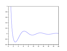
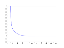
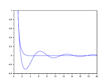
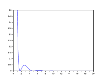
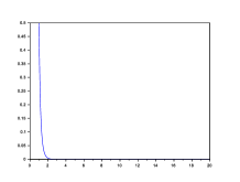
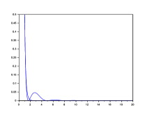
Figure 1. Up: $(t,x(t))$ for AVD (left), DIN-AVD (middle), both (right). Down: $(t,\Phi(x(t)))$ for AVD (left), DIN-AVD (middle), both (right).

Illustration 1.17.

Now, we consider the function $\Phi(x,y)=\frac{1}{2}(x^{2}+1000y^{2})$, which is still quadratic but not well conditioned. Figure 2 shows the curves $(x(t),y(t))$ and $(t,\Phi(x(t),y(t)))$. As before, we show the behavior on the interval $[1,20]$ with $\alpha=3.1$ and, for (DIN-AVD), $\beta=1$. The initial conditions were $(x(1),y(1))=(1,1)$ and $(\dot{x}(1),\dot{y}(1))=(0,0)$. In both cases, the trajectories and the function values converge to the global minimum $(0,0)$ and the optimal value $0$, respectively. However, the wild transversal oscillation exhibited by the solution of (AVD) are neutralized by (DIN-AVD).

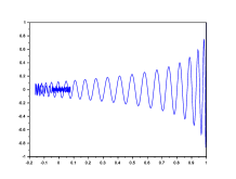
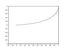
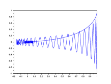
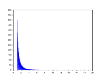
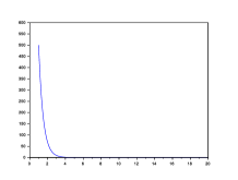
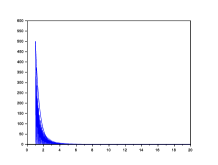
Figure 2. Up: $(x(t),y(t))$ for AVD (left), DIN-AVD (middle), both (right). Down: $(t,\Phi(x(t),y(t)))$ for AVD (left), DIN-AVD (middle), both (right).

2. Strong convergence results

In this section, we establish strong convergence of the trajectories in several relevant cases, namely: when $\Phi$ is even, uniformly convex, boundedly inf-compact, or if $\hbox{int}({\rm argmin}\kern 1.19995pt\Phi)\neq\emptyset$.

2.1. Even objective function

Recall that $\Phi$ is even if $\Phi(x)=\Phi(-x)$ for all $x\in\mathcal{H}$.

Theorem 2.1.

Suppose $\alpha>3$, $\beta>0$ and let $\Phi$ be twice differentiable, convex and even. Let $x:[t_{0},+\infty[\rightarrow\mathcal{H}$ be the global classical solution to (DIN-AVD) with Cauchy data $x(t_{0})=x_{0}$ and $\dot{x}(t_{0})=\dot{x}_{0}$. Then, $x(t)$ converges strongly, as $t\to+\infty$, to some $x^{*}\in{\rm argmin}\kern 1.19995pt\Phi$.

Proof.

Let $t_{1}>t_{0}$ and for $t_{0}\leq t\leq t_{1}$ define the following function of $t$

(26) $$g(t)=\|x(t)\|^{2}-\|x(t_{1})\|^{2}-\frac{1}{2}\|x(t)-x(t_{1})\|^{2}-\int_{t}^{t_{1}}\langle\beta\nabla\Phi(x(s)),x(s)+x(t_{1})\rangle ds.$$

We have

$$\dot{g}(t) =\langle\dot{u}_{\beta}(t),x(t)+x(t_{1})\rangle$$

$$\ddot{g}(t) =\langle\ddot{u}_{\beta}(t),x(t)+x(t_{1})\rangle+\langle\dot{u}_{\beta}(t),\dot{x}(t)\rangle,$$

where, we recall, $u_{\beta}$ is defined by (8) with $\theta=\beta$. Combining the two equations above, and using (13) we obtain

(27) $$\ddot{g}(t)+\frac{\alpha}{t}\dot{g}(t)=\langle\dot{u}_{\beta}(t),\dot{x}(t)\rangle-\left(1-\frac{\alpha\beta}{t}\right)\langle\nabla\Phi(x(t)),x(t)+x(t_{1})\rangle.$$

The energy function $W_{\beta}(t)=\frac{1}{2}\|\dot{u}_{\beta}(t)\|^{2}+\Phi(x(t))$ is nonincreasing by Proposition 1.2. Comparing the values of $W_{\beta}$ at $t$ and $t_{1}$, and successively using the fact that $\Phi$ is even along with the convex differential inequality, we obtain

$$\frac{1}{2}\|\dot{u}_{\beta}(t)\|^{2}+\Phi(x(t)) \geq\frac{1}{2}\|\dot{u}_{\beta}(t_{1})\|^{2}+\Phi(x(t_{1}))$$

$$=\frac{1}{2}\|\dot{u}_{\beta}(t_{1})\|^{2}+\Phi(-x(t_{1}))$$

$$\geq\frac{1}{2}\|\dot{u}_{\beta}(t_{1})\|^{2}+\Phi(x(t))-\langle\nabla\Phi(x(t)),x(t)+x(t_{1})\rangle.$$

After simplification, we obtain

$$-\langle\nabla\Phi(x(t)),x(t)+x(t_{1})\rangle\leq\frac{1}{2}\|\dot{u}_{\beta}(t)\|^{2}.$$

Since we are interested in the asymptotic behaviour of $x$, there is no harm in supposing $t\geq\alpha\beta$; so we deduce from the inequality above that

$$-\left(1-\frac{\alpha\beta}{t}\right)\langle\nabla\Phi(x(t)),x(t)+x(t_{1})\rangle\leq\left(1-\frac{\alpha\beta}{t}\right)\frac{1}{2}\|\dot{u}_{\beta}(t)\|^{2}\leq\frac{1}{2}\|\dot{u}_{\beta}(t)\|^{2}.$$

Then, equality (27) yields

$$\ddot{g}(t)+\frac{\alpha}{t}\dot{g}(t)\leq\langle\dot{u}_{\beta}(t),\dot{x}(t)\rangle+\frac{1}{2}\|\dot{u}_{\beta}(t)\|^{2}.$$

Using (9), it ensues that

$$\ddot{g}(t)+\frac{\alpha}{t}\dot{g}(t) \leq \frac{3}{2}\|\dot{x}(t)\|^{2}+2\langle\beta\nabla\Phi(x(t)),\dot{x}(t)\rangle+\frac{1}{2}\|\beta\nabla\Phi(x(t))\|^{2}$$

$$\leq \frac{5}{2}\|\dot{x}(t)\|^{2}+\frac{3}{2}\|\beta\nabla\Phi(x(t))\|^{2}.$$

Multiply the latter inequality by t and integrate from $t$ to $t_{1}\geq t$ to obtain

$$t_{1}\dot{g}(t_{1})-t\dot{g}(t)-(\alpha-1)g(t)\leq\frac{5}{2}\int_{t}^{t_{1}}s\|\dot{x}(s)\|^{2}ds+\frac{3}{2}\int_{t}^{t_{1}}s\|\beta\nabla\Phi(x(s))\|^{2}ds.$$

Let us take the definition of $g$ (26) into account to obtain

$$(\alpha-1)\frac{1}{2}\|x(t)-x(t_{1})\|^{2} \leq (\alpha-1)(\|x(t)\|^{2}-\|x(t_{1})\|^{2})-(\alpha-1)\int_{t}^{t_{1}}\langle\beta\nabla\Phi(x(s)),x(s)+x(t_{1})\rangle ds$$

$$+(t\dot{g}(t)-t_{1}\dot{g}(t_{1}))+\frac{5}{2}\int_{t}^{t_{1}}s\|\dot{x}(s)\|^{2}ds+\frac{3}{2}\int_{t}^{t_{1}}s\|\beta\nabla\Phi(x(s))\|^{2}ds.$$

Now, we have the following convergence results, as $t$ and $t_{1}$ tend to $+\infty$ with $t\leq t_{1}$:

• Since $0\in{\rm argmin}\kern 1.19995pt\Phi$, part (iii) of Lemma 1.13 implies $\|x(t)\|$ has a limit as $t\to+\infty$. Therefore, $(\|x(t)\|^{2}-\|x(t_{1})\|^{2})$ vanishes;

• Proposition 1.11 implies $t\mapsto\|\nabla\Phi(x(t))\|=\frac{1}{t}\times t\|\nabla\Phi(x(t))\|$ belongs to $L^{1}(t_{0},+\infty)$, as a product of functions in $L^{2}(t_{0},+\infty)$. Since $x$ is bounded, $s\mapsto\langle\beta\nabla\Phi(x(s)),x(s)+x(t_{1})$ is in $L^{1}(t_{0},+\infty)$, and so $\int_{t}^{t_{1}}\langle\beta\nabla\Phi(x(s)),x(s)+x(t_{1})\rangle ds$ vanishes;

• $|t\dot{g}(t)|=|t\langle\dot{x}(t)+\beta\nabla\Phi(x(t)),x(t)+x(t_{1})\rangle|$, this last quantity vanishes in view of Theorem 1.15 and the boundedness of $x$;

• $\int_{t}^{t_{1}}s\|\dot{x}(s)\|^{2}ds$ vanishes in view of part (i) of Lemma 1.13;

• $\int_{t}^{t_{1}}s\|\beta\nabla\Phi(x(s))\|^{2}ds$ vanishes in view of Proposition 1.11.

As a consequence, as $t\to+\infty$, $x(t)$ satisfies the Cauchy criterion in the Hilbert space $\mathcal{H}$. The limit obviously is a minimum point by Corollary 1.4. ∎

2.2. Solution set with nonempty interior

In this subsection, we examine the case where $\hbox{int}({\rm argmin}\kern 1.19995pt\Phi)\neq\emptyset$.

Theorem 2.2.

Suppose $\alpha>3$, $\beta>0$ and let $\Phi$ satisfy int$({\rm argmin}\kern 1.19995pt\Phi)\neq\emptyset$. Let $x$ be a classical global solution of (DIN-AVD). Then, $x(t)$ converges strongly, as $t\to+\infty$, to some $x^{*}\in{\rm argmin}\kern 1.19995pt\Phi$. Moreover,

$$\int_{t_{0}}^{\infty}t\|\nabla\Phi(x(t))\|dt<+\infty.$$

Proof.

Since int$({\rm argmin}\kern 1.19995pt\Phi)\neq\emptyset$, there exist $\xi^{*}\in{\rm argmin}\kern 1.19995pt\Phi$ and $\rho>0$ such that$\{z\in\mathcal{H},\;\|z-\xi^{*}\|<\rho\}\subseteq{\rm argmin}\kern 1.19995pt\Phi$. According to the monotonicity of $\nabla\Phi$, for any $y\in\mathcal{H}$ and any $z\in\mathcal{H}$ such that $\|z-\xi^{*}\|<\rho$, we have

$$\langle\nabla\Phi(y),y-z\rangle\geq 0.$$

Hence

$$\langle\nabla\Phi(y),y-\xi^{*}\rangle\geq\langle\nabla\Phi(y),z-\xi^{*}\rangle.$$

Taking the supremum with respect to $z\in\mathcal{H}$ such that $\|z-\xi^{*}\|<\rho$, we infer that for any $y\in\mathcal{H}$, we have

(28) $$\langle\nabla\Phi(y),y-\xi^{*}\rangle\geq\rho\|\nabla\Phi(y)\|.$$

In particular taking $y=x(t)$, we obtain

(29) $$\langle\nabla\Phi(x(t)),x(t)-\xi^{*}\rangle\geq\rho\|\nabla\Phi(x(t))\|.$$

From part (ii) of Lemma 1.13, we deduce that

(30) $$\rho\int_{t_{0}}^{\infty}t\|\nabla\Phi(x(t))\|dt\leq\int_{t_{0}}^{\infty}t\langle x(t)-\xi^{*},\nabla\Phi(x(t))dt<\infty.$$

Multiply equation (13) (with $\theta=\beta$) by $t$ to obtain

$$t\ddot{u}_{\beta}(t)+\alpha\dot{u}_{\beta}(t)=(\alpha\beta-t)\nabla\Phi(x(t)),$$

and integrate between $t_{0}$ and $t\geq t_{0}$ to conclude that

$$t\dot{u}_{\beta}(t)+(\alpha-1)u_{\beta}(t)=t_{0}\dot{u}_{\beta}(t_{0})+(\alpha-1)u_{\beta}(t_{0})+\int_{t_{0}}^{t}(\alpha\beta-s)\nabla\Phi(x(s))ds.$$

In view of (30) the right-hand side has a limit as $t\to+\infty$. —With Lemma 7.2, $u_{\beta}(t)=x(t)+\int_{t_{0}}^{t}\beta\nabla\Phi(x(s))ds$ has a limit as well. Hence $x(t)$ has a limit, which is a minimum point of $\Phi$. ∎

Let us notice that, thanks to the assumption $\mbox{int}({\rm argmin}\kern 1.19995pt\Phi)\neq\emptyset$, we have been able to pass from the $L^{2}$ estimation of Proposition 1.11 to an $L^{1}$ estimate for $t\mapsto t\|\nabla\Phi(x(t))\|$.

2.3. Bounded inf-compactness

A function $\Phi:\mathcal{H}\rightarrow\mathbb{R}$ is boundedly inf-compact if, for any $\lambda\in\mathbb{R}$, and $R>0$, the set  $\left\{x\in\mathcal{H}:\ \Phi(x)\leq\lambda,\ \|x\|\leq R\right\}$  is relatively compact in $\mathcal{H}$.

Theorem 2.3.

Suppose $\alpha\geq 3$ and that $\Phi:\mathcal{H}\rightarrow\mathbb{R}$ is a boundedly inf-compact function with ${\rm argmin}\kern 1.19995pt\Phi\neq\emptyset$. Then, every trajectory $x$ of (DIN-AVD) converges strongly, as $t\to+\infty$, to some $x^{*}\in{\rm argmin}\kern 1.19995pt\Phi$.

Proof.

The trajectory $x$ is minimizing by Theorem 1.3, and bounded by Theorem 1.10. Consequently, the trajectory is contained in the intersection of a sublevel set of $\Phi$ with some ball, which must be a compact set, since $\Phi$ is boundedly inf-compact. The trajectory converges weakly and is contained in a compact set. Hence it converges strongly to some $x^{*}\in{\rm argmin}\kern 1.19995pt\Phi$. ∎

2.4. Uniform convexity/monotonicity

Following [15], we say that $\nabla\Phi$ is uniformly monotone on bounded sets, if, for each $r>0$, there exists a nondecreasing function $\omega_{r}:[0,+\infty[\to[0,+\infty[$ vanishing only at 0, and such that

$$\langle\nabla\Phi(x)-\nabla\Phi(y),x-y\rangle\geq\omega_{r}(\|x-y\|)$$

for all $x,y\in\mathcal{H}$ with $\|x\|\leq r,\|y\|\leq r$.

Theorem 2.4.

Suppose $\alpha>3$, $\beta>0$. Suppose that ${\rm argmin}\kern 1.19995pt\Phi\neq\emptyset$, and $\nabla\Phi$ is uniformly monotone on bounded sets. Let $x$ be a classical global solution of (DIN-AVD). Then, ${\rm argmin}\kern 1.19995pt\Phi$ is reduced to a singleton $x^{*}$, and $x(t)$ converges strongly to $x^{*}$, as $t\to+\infty$.

Proof.

If $x^{*}$ and $x^{**}$ are two minimum points, then for $r=\max\{\|x^{*}\|,\|x^{**}\|\}$, we must have $\omega_{r}(\|x^{*}-x^{**}\|)=0$; hence ${\rm argmin}\kern 1.19995pt\Phi$, which is nonempty, reduces to one point, say, $x^{*}$.

By Theorem 1.10, the trajectory $x$ is bounded. Let $r>0$ be such that it is contained in the ball centered at the origin with radius $r$. Since $\nabla\Phi$ is uniformly monotone on bounded sets, and $\nabla\Phi(x^{*})=0$, we have

$$\langle\nabla\Phi(x(t)),x(t)-x^{*}\rangle\geq\omega_{r}(\|x(t)-x^{*}\|).$$

Hence

$$\omega_{r}(\|x(t)-x^{*}\|)\leq 2r\|\nabla\Phi(x(t))\|.$$

By Proposition 1.5,

$$\lim_{t\to\infty}\|\nabla\Phi(x(t))\|=0.$$

Hence $\omega_{r}(\|x(t)-x^{*}\|)\to 0$, which implies $\|x(t)-x^{*}\|\rightarrow 0$. ∎

3. Further results in the strongly convex case

Let us recall that a function $\Phi:\mathcal{H}\rightarrow\mathbb{R}$ is strongly convex if there exists some $\mu>0$ such that the function $\Phi-(\mu/2)\|\cdot\|^{2}$ is convex. If $\Phi$ is differentiable, the convexity inequality yields, for all $x,y\in\mathcal{H}$

$$\Phi(y)-\frac{\mu}{2}\|y\|^{2}\geq\Phi(x)-\frac{\mu}{2}\|x\|^{2}+\langle\nabla\Phi(x)-\mu x,y-x\rangle.$$

Whence, for all $x,y\in\mathcal{H}$

(31) $$\Phi(y)\geq\Phi(x)+\langle\nabla\Phi(x),y-x\rangle+\frac{\mu}{2}\|x-y\|^{2}.$$

The gradient of a strongly convex function is uniformly monotone on bounded sets, so that Theorem 2.4 holds. However, in the case of a strongly convex function, we can obtain a rate of convergence for $\Phi(x(t))$ to the infimal value better than that of Theorem 1.10 and more precise than that of Theorem 1.15.

Theorem 3.1.

Suppose $\alpha\geq 3$ and that $\Phi:\mathcal{H}\to{\mathbb{R}}$ is strongly convex. Then, ${\rm argmin}\kern 1.19995pt\Phi$ is reduced to a singleton $x^{*}$, and for any trajectory $x$ of (DIN-AVD) the following properties hold:

$$\Phi(x(t))-\min_{\mathcal{H}}\Phi = \mathcal{O}\left(t^{-\frac{2\alpha}{3}}\right)$$

$$\|x(t)-x^{*}\| = O\left(t^{-\frac{\alpha}{3}}\right).$$

Proof.

The first part follows from Theorem 2.4. For the convergence rates, the proof goes along the lines of that of Theorem 1.10: we shall show that a surrogate Lyapunov function (namely, the function $\mathcal{L}$ defined below) is bounded. Let $p\in{\mathbb{R}}$, $\lambda>0$ and let $Q$ be a quadratic polynomial. Precise values, depending on $\alpha$ and $\beta$, will be given further to $\lambda$, $p$, $Q$. Let us briefly write $u$ for $u_{\beta}$. Set $P(t)=t^{p}$ and for $x^{*}\in{\rm argmin}\kern 1.19995pt\Phi$ define

$$\mathcal{L}_{0}(t) = Q(t)(\Phi(x(t))-\Phi(x^{*}))+\frac{1}{2}\|\lambda(x(t)-x^{*})+t\dot{u}(t)\|^{2}$$

$$\mathcal{L}(t) = P(t)\mathcal{L}_{0}(t).$$

Our first task is to differentiate function $\mathcal{L}$. To simplify the wording, we write $\Phi^{*}$ for $\Phi(x^{*})$ and the dependence of $x$, $P$, $Q$, $\mathcal{L}_{0}$ and $\mathcal{L}$ on $t$ is not made explicit. To compute $d\mathcal{L}_{0}/dt$, we make use of (9) and (10).

$$\frac{d\mathcal{L}_{0}}{dt}=\, \dot{Q}(\Phi(x)-\Phi^{*})+Q\langle\dot{x},\nabla\Phi(x)\rangle+\langle\lambda(x-x^{*})+t\dot{u},\lambda\dot{x}+\dot{u}+t\ddot{u}\rangle$$

$$=\, \dot{Q}(\Phi(x)-\Phi^{*})+Q\langle\dot{x},\nabla\Phi(x)\rangle+\langle\lambda(x-x^{*})+t\dot{x}+t\beta\nabla\Phi(x)),(\lambda+1-\alpha)\dot{x}+(\beta-t)\nabla\Phi(x)\rangle$$

$$=\, \dot{Q}(\Phi(x)-\Phi^{*})+(Q-t^{2}+\beta(\lambda+2-\alpha)t)\langle\dot{x},\nabla\Phi(x)\rangle+\lambda(\lambda+1-\alpha)\langle x-x^{*},\dot{x}\rangle+\lambda(\beta-t)\langle x-x^{*},\nabla\Phi(x)\rangle$$

$$+(\lambda+\alpha-1)t\|\dot{x}\|^{2}+\beta t(\beta-t)\|\nabla\Phi(x)\|^{2}.$$

Expand $\mathcal{L}_{0}$ as

$$\mathcal{L}_{0}=\, Q(\Phi(x)-\Phi^{*})+\frac{\lambda^{2}}{2}\|x-x^{*}\|^{2}+\frac{t^{2}}{2}\|\dot{x}\|^{2}+\frac{\beta^{2}t^{2}}{2}\|\nabla\Phi(x)\|^{2}+\lambda t\langle x-x^{*},\dot{x}\rangle+\lambda\beta t\langle x-x^{*},\nabla\Phi(x)\rangle+\beta t^{2}\langle\dot{x},\nabla\Phi(x)\rangle,$$

and compute

$$\frac{d\mathcal{L}}{dt}=\, \frac{d\mathcal{L}_{0}}{dt}P+\mathcal{L}_{0}\dot{P}$$

(32) $$=\, \frac{d(PQ)}{dt}(\Phi(x)-\Phi^{*})+[(Q-t^{2}+\beta(\lambda+2-\alpha)t)P+\beta t^{2}\dot{P}]\langle\dot{x},\nabla\Phi(x)\rangle$$

$$+[\lambda(\lambda+1-\alpha)P+\lambda t\dot{P}]\langle x-x^{*},\dot{x}\rangle+\lambda[(\beta-t)P+\beta t\dot{P}]\langle x-x^{*},\nabla\Phi(x)\rangle+[2(\lambda+1-\alpha)tP+t^{2}\dot{P}]\frac{1}{2}\|\dot{x}\|^{2}$$

$$+[2\beta(\beta-t)tP+\beta^{2}t^{2}\dot{P}]\frac{1}{2}\|\nabla\Phi(x)\|^{2}+\frac{\lambda^{2}\dot{P}}{2}\|x-x^{*}\|^{2}.$$

For $t$ large enough (namely $t>(p+1)\beta$) the coefficient $\lambda[(\beta-t)P+\beta t\dot{P}]$ of $\langle x-x^{*},\nabla\Phi(x)\rangle$ is negative. Applying the strong convexity inequality (31) (with $y=x^{*}$), we have

$$\lambda[(\beta-t)P+\beta t\dot{P}]\langle x-x^{*},\nabla\Phi(x)\rangle\leq\lambda[(\beta-t)P+\beta t\dot{P}](\Phi(x)-\Phi^{*})+\lambda[(\beta-t)P+\beta t\dot{P}]\frac{\mu}{2}\|x-x^{*}\|^{2}.$$

So, we can dispose of $\langle x-x^{*},\nabla\Phi(x)\rangle$ in (32), and obtain the inequality

(33) $$\frac{d\mathcal{L}}{dt}\leq\, \left[\frac{d(PQ)}{dt}+\lambda((\beta-t)P+\beta t\dot{P})\right](\Phi(x)-\Phi^{*})+[(Q-t^{2}+\beta(\lambda+2-\alpha)t)P+\beta t^{2}\dot{P}]\langle\dot{x},\nabla\Phi(x)\rangle$$

$$+[\lambda(\lambda+1-\alpha)P+\lambda t\dot{P}]\langle x-x^{*},\dot{x}\rangle+[2(\lambda+1-\alpha)tP+t^{2}\dot{P}]\frac{1}{2}\|\dot{x}\|^{2}$$

$$+[2\beta(\beta-t)tP+\beta^{2}t^{2}\dot{P}]\frac{1}{2}\|\nabla\Phi(x)\|^{2}+[\lambda^{2}\dot{P}+\mu\lambda((\beta-t)P+\beta t\dot{P})]\frac{1}{2}\|x-x^{*}\|^{2}.$$

If we choose $p=2(\alpha-1-\lambda)$ and $Q(t)=t^{2}-\beta(\lambda+2-\alpha+p)t=t^{2}-\beta(\alpha-\lambda)t$, the coefficients of $\|\dot{x}\|$ and $\langle\dot{x},\nabla\Phi(x)\rangle$ vanish (recall $P(t)=t^{p}$). Taking these facts into account, we deduce from (33) that

$$\frac{d\mathcal{L}}{dt}\leq\, -t^{p}[(\lambda-2-p)t+\beta(\alpha-2\lambda)(p+1)](\Phi(x)-\Phi^{*})+\lambda(\lambda+1-\alpha+p)t^{p}\langle x-x^{*},\dot{x}\rangle$$

$$-\beta t^{p+1}[2t-\beta(p+2)]\frac{1}{2}\|\nabla\Phi(x)\|^{2}-\lambda t^{p-1}[\mu t^{2}-\mu\beta(p+1)t-p\lambda]\frac{1}{2}\|x-x^{*}\|^{2}.$$

For $t$ sufficiently large, the coefficients of $\|\nabla\Phi(x)\|^{2}$ and $\|x-x^{*}\|^{2}$ are negative; hence

(34) $$\frac{d\mathcal{L}}{dt}\leq\, -t^{p}[(\lambda-2-p)t+\beta(\alpha-2\lambda)(p+1)](\Phi(x)-\Phi^{*})+\lambda(\lambda+1-\alpha+p)t^{p}\langle x-x^{*},\dot{x}\rangle.$$

Choose $\lambda=\frac{2}{3}\alpha$, whence $p=\frac{2}{3}\alpha-2$, $\lambda-2-p=0$. Moreover, define $h(t)=\frac{1}{2}\|x(t)-x^{*}\|^{2}$. Then inequality (34) becomes

(35) $$\frac{d\mathcal{L}}{dt}\leq\, \frac{\alpha\beta}{9}(2\alpha-3)t^{p}(\Phi(x)-\Phi^{*})+\frac{2\alpha}{9}(\alpha-3)t^{p}\dot{h}.$$

To simplify the notations, set $\gamma=\frac{\alpha\beta}{9}(2\alpha-3)$ and $\delta=\frac{\alpha\beta}{3}$, and notice that $Q(t)=t(t-\delta)$ and $\frac{2\alpha}{9}(\alpha-3)=\frac{p\alpha}{3}$. Inequality (35) reads

$$\frac{d\mathcal{L}}{dt}\leq\, \gamma t^{p}(\Phi(x)-\Phi^{*})+\frac{p\alpha}{3}t^{p}\dot{h}.$$

With $t^{p}Q(\Phi(x)-\Phi^{*})\leq\mathcal{L}$ (for $t>\delta$), the inequality above becomes

$$\frac{d\mathcal{L}}{dt}\leq\, \gamma\frac{\mathcal{L}}{Q}+\frac{p\alpha}{3}t^{p}\dot{h}.$$

If we multiply this inequality by $(\frac{t}{t-\delta})^{p+1}$ we obtain

$$\left(\frac{t}{t-\delta}\right)^{p+1}\left[\frac{d\mathcal{L}}{dt}-\gamma\frac{\mathcal{L}}{Q}\right]=\frac{d}{dt}\left[\left(\frac{t}{t-\delta}\right)^{p+1}\mathcal{L}\right]\leq\frac{p\alpha}{3}t^{p}\left(\frac{t}{t-\delta}\right)^{p+1}\dot{h}.$$

Integrating between $t_{1}$, sufficiently large, and $t\geq t_{1}$, we obtain

$$\left(\frac{t}{t-\delta}\right)^{p+1}\mathcal{L}(t))\leq$$

$$\left(\frac{t_{1}}{t_{1}-\delta}\right)^{p+1}\mathcal{L}(t_{1})+\frac{p\alpha}{3}\left[t^{p}\left(\frac{t}{t-\delta}\right)^{p+1}h(t)-t_{1}^{p}\left(\frac{t_{1}}{t_{1}-\delta}\right)^{p+1}h(t_{1})-\int_{t_{1}}^{t}\frac{d}{ds}\left[s^{p}\left(\frac{s}{s-\delta}\right)^{p+1}\right]h(s)ds\right].$$

But $\frac{d}{ds}\ln(s^{p}(\frac{s}{s-\delta})^{p+1})=\frac{ps-\gamma}{s(s-\delta)}$, which shows that the integrand is positive for $t$ large enough. Hence

$$\left(\frac{t}{t-\delta}\right)^{p+1}\mathcal{L}(t))\leq\left(\frac{t_{1}}{t_{1}-\delta}\right)^{p+1}\mathcal{L}(t_{1})+\frac{p\alpha}{3}t^{p}\left(\frac{t}{t-\delta}\right)^{p+1}h(t).$$

Whence, we deduce that

(36) $$\mathcal{L}(t))\leq\left(\frac{t-\delta}{t}\right)^{p+1}\left(\frac{t_{1}}{t_{1}-\delta}\right)^{p}\mathcal{L}(t_{1})+\frac{p\alpha}{3}t^{p}h(t)\leq\left(\frac{t_{1}}{t_{1}-\delta}\right)^{p}\mathcal{L}(t_{1})+\frac{p\alpha}{3}t^{p}h(t).$$

Now, in view of the strong convexity inequality (31) (with $x=x^{*}$ and $y=x(t)$) we have

(37) $$h(t)\leq\frac{1}{\mu}(\Phi(x(t))-\Phi^{*})\leq\frac{\mathcal{L}(t)}{\mu t^{p}Q(t)}.$$

Hence, inequality (36) yields

$$\mathcal{L}(t))\leq\left(\frac{t_{1}}{t_{1}-\delta}\right)^{p}\mathcal{L}(t_{1})+\frac{p\alpha}{3\mu}\frac{\mathcal{L}(t)}{Q(t)}.$$

We deduce that

$$\mathcal{L}(t))\leq\left(\frac{t_{1}}{t_{1}-\delta}\right)^{p+1}\mathcal{L}(t_{1})\frac{Q(t)}{Q(t)-\frac{p\alpha}{3\mu}},$$

which shows that $\mathcal{L}$ is bounded.

If $L$ denotes an upper bound of $\mathcal{L}$, we have

$$\Phi(x(t))-\Phi^{*}\leq\frac{L}{t^{p}Q(t)}=\mathcal{O}\left(\frac{1}{t^{p+2}}\right)=\mathcal{O}\left(t^{-\frac{2\alpha}{3}}\right).$$

In view of the first inequality in (37), we also have

$$\|x(t)-x^{*}\|=\mathcal{O}\left(t^{-\frac{\alpha}{3}}\right),$$

as claimed. ∎

4. (DIN-AVD) as a first-order system. Extension to non-smooth potentials

Let $\beta>0$. As we shall see, the presence of the Hessian damping term allows formulating (DIN-AVD) as a first-order system both in time and space (with no occurrence of the Hessian). This will allow us to extend our study to the case of a proper lower-semicontinuous convex function, by simply replacing the gradient by the subdifferential. This approach was initiated in [6] in the case of (DIN), and further exploited for the study of damped shocks in mechanics in [11].

We begin by establishing the equivalence between (DIN-AVD) and a first-order system in the smooth case in Subsection 4.1, and then recover most results from preceding sections in the nonsmooth setting. Some of the arguments are essentially the same, so we will study in more detail the parts that are not, and leave the rest to the reader. To simplify the reading, we shall use $\Phi$ to denote a smooth potential (as in the previous sections), and $\phi$ for a proper lower-semicontinuous convex function.

4.1. (DIN-AVD) as a first-order system

Theorem 4.1.

Let $\Phi:\mathcal{H}\rightarrow\mathbb{R}$ be twice continuously differentiable. Suppose $\alpha\geq 0$, $\beta>0$. Let $(x_{0},\dot{x}_{0})\in\mathcal{H}\times\mathcal{H}$. The following statements are equivalent:

1. $x:[t_{0},+\infty[\to\mathcal{H}$ is a solution to the second-order differential equation

   $${\hbox{\rm(DIN-AVD)}}\quad\quad\ddot{x}(t)+\frac{\alpha}{t}\dot{x}(t)+\beta\nabla^{2}\Phi(x(t))\dot{x}(t)+\nabla\Phi(x(t))=0,$$

   with initial conditions $x(t_{0})=x_{0}$, $\dot{x}(t_{0})=\dot{x}_{0}$.

2. $(x,y):[t_{0},+\infty[\to\mathcal{H}\times\mathcal{H}$ is a solution to the first-order system

   $${\hbox{\rm(DIN-AVD)}_{f}}\ \left\{\begin{array}[]{rcl}\dot{x}(t)+\beta\nabla\Phi(x(t))-\left(\frac{1}{\beta}-\frac{\alpha}{t}\right)x(t)+\frac{1}{\beta}y(t)&=&0\\ \dot{y}(t)-\left(\frac{1}{\beta}-\frac{\alpha}{t}+\frac{\alpha\beta}{t^{2}}\right)x(t)+\frac{1}{\beta}y(t)&=&0,\end{array}\right.$$

   with initial conditions $x(t_{0})=x_{0}$, $y(t_{0})=-(\dot{x}_{0}+\beta\nabla\Phi(x_{0}))/\beta+(1-\beta\alpha/t_{0})x_{0}$.

Proof.

To simplify the notation, set $a(t)=\alpha/t$ and $z(t)=\int_{t_{0}}^{t}(a(s)\dot{x}(s)+\nabla\Phi(x(s)))ds-(\dot{x}_{0}+\beta\nabla\Phi(x_{0}))$.

Integrating (DIN-AVD) from $t_{0}$ to $t\geq t_{0}$ and differentiating $z$, we see that $x$ is a solution to (DIN-AVD) with initial conditions $x(t_{0})=x_{0}$, $\dot{x}(t_{0})=\dot{x}_{0}$, if and only if, $(x,z)$ is a solution to

(38) $$\left\{\begin{array}[]{rcl}\dot{x}(t)+\beta\nabla\Phi(x(t))+z(t)&=&0\\ \dot{z}(t)-a(t)\dot{x}(t)-\nabla\Phi(x(t))&=&0,\end{array}\right.$$

with initial conditions $x(t_{0})=x_{0}$, $z(t_{0})=-(\dot{x}_{0}+\beta\nabla\Phi(x_{0}))$.

Use a linear combination of the rows in (38) to eliminate the gradient in the second equation, and obtain the equivalent system

(39) $$\left\{\begin{array}[]{rcl}\dot{x}(t)+\beta\nabla\Phi(x(t))+z(t)&=&0\\ \beta\dot{z}(t)+(1-\beta a(t))\dot{x}(t)+z(t)&=&0.\end{array}\right.$$

Now define $y(t)=\beta z(t)+(1-\beta a(t))x(t)$. We see that $(x,z)$ is a solution to (39), with initial conditions $x(t_{0})=x_{0}$, $z(t_{0})=-(\dot{x}_{0}+\beta\nabla\Phi(x_{0}))$, if and only if $(x,y)$ is a solution to

$$\left\{\begin{array}[]{rcl}\dot{x}(t)+\beta\nabla\Phi(x(t))-\left(\frac{1}{\beta}-a(t)\right)x(t)+\frac{1}{\beta}y(t)&=&0\\ \dot{y}(t)+\beta\dot{a}(t)x(t)-\left(\frac{1}{\beta}-a(t)\right)x(t)+\frac{1}{\beta}y(t)&=&0,\end{array}\right.$$

with initial conditions $x(t_{0})=x_{0}$, $y(t_{0})=-\beta(\dot{x}_{0}+\beta\nabla\Phi(x_{0}))+(1-\beta\ a(t_{0}))x_{0}$. ∎

4.2. Existence of solutions in a nonsmooth setting

Beyond being of first-order in time, $\hbox{\rm(DIN-AVD)}_{f}$ does not involve the Hessian of $\Phi$. As a first consequence, the numerical solution of (DIN-AVD) is highly simplified, since it may be performed by discretization of $\hbox{\rm(DIN-AVD)}_{f}$ and only requires approximating the gradient of $\Phi$. Next, $\hbox{\rm(DIN-AVD)}_{f}$ permits to give a meaning to (DIN-AVD) even when $\Phi$ is not twice differentiable. In particular, we may consider a proper lower-semicontinuous convex potential function $\phi$.

More precisely, we have the following:

Definition 4.2.

Let $\alpha\geq 0$, $\beta>0$ and $\phi:\mathcal{H}\to{\mathbb{R}}\cup\{+\infty\}$ be a proper lower-semicontinuous convex function. The generalized (DIN-AVD) system, (g-DIN-AVD) for short, is defined by

(40) $$\hbox{\rm(g-DIN-AVD)}\ \left\{\begin{array}[]{rcl}\dot{x}(t)+\beta\partial\phi(x(t))-\left(\frac{1}{\beta}-\frac{\alpha}{t}\right)x(t)+\frac{1}{\beta}y(t)&\ni&0\\ \dot{y}(t)-\left(\frac{1}{\beta}-\frac{\alpha}{t}+\frac{\alpha\beta}{t^{2}}\right)x(t)+\frac{1}{\beta}y(t)&=&0,\end{array}\right.$$

where $\partial\phi$ stands for the convex subdifferential of $\phi$.

Setting $Z(t)=(x(t),y(t))\in\mathcal{H}\times\mathcal{H}$, (g-DIN-AVD) can be equivalently written

(41) $$\dot{Z}(t)+\partial\mathcal{G}(Z(t))+D(t,Z(t))\ni 0,$$

where $\mathcal{G}:\mathcal{H}\times\mathcal{H}\rightarrow\mathbb{R}\cup\{+\infty\}$ is the convex function defined by

(42) $$\mathcal{G}(Z)=\mathcal{G}(x,y)=\beta\phi(x),$$

and $D:\ [t_{0},+\infty[\times\mathcal{H}\times\mathcal{H}\to\mathcal{H}\times\mathcal{H}$ is given by

(43) $$D(t,Z)=D(t,x,y)=\left(-\left(\frac{1}{\beta}-\frac{\alpha}{t}\right)x+\frac{1}{\beta}y,-\left(\frac{1}{\beta}-\frac{\alpha}{t}+\frac{\alpha\beta}{t^{2}}\right)x+\frac{1}{\beta}y\right).$$

The differential inclusion (41) is governed by the sum of the maximal monotone operator $\partial\mathcal{G}$ (a convex subdifferential) and the time-dependent linear continuous operator $D(t,\cdot)$. The existence and uniqueness of a global solution for the corresponding Cauchy problem is a consequence of the general theory of evolution equations governed by maximal monotone operators. Before giving a precise statement, let us recall the notion of strong solution (see [17, Definition 3.1]).

Definition 4.3.

Let $\mathcal{H}$ be a Hilbert space, $t_{0}\in{\mathbb{R}}$ and $T>t_{0}$. Consider a proper lower-semicontinuous convex function $\phi:\mathcal{H}\to{\mathbb{R}}\cup\{+\infty\}$, along with a function $B:[t_{0},+\infty[\times\mathcal{H}\to\mathcal{H}$. We say that $z:[t_{0},T]\to\mathcal{H}$ is a strong solution on $[t_{0},T]$ to the differential inclusion

(44) $$\dot{z}(t)+\partial\phi(z(t))+B(t,z(t))\ni 0,$$

if the following properties are satisfied:

1. $z\in\mathcal{C}([t_{0},T],\mathcal{H})$;

2. $z$ is absolutely continuous on any compact subset of $]t_{0},T]$;

3. $z(t)\in\mbox{dom}(\partial\phi)$ for almost every $t\in]t_{0},T]$;

4. the inclusion (44) is verified for almost every $t\in]t_{0},T]$.

We say that $z:[t_{0},+\infty[\to\mathcal{H}$ is a global strong solution to (44), if it is a strong solution to (44) on $[t_{0},T]$ for all $T>t_{0}$.

With this terminology, we have the following:

Theorem 4.4.

Let $\phi:\mathcal{H}\rightarrow\mathbb{R}\cup\{+\infty\}$ be a convex lower semicontinuous proper function, and let $\beta>0$. For any Cauchy data $(x_{0},y_{0})\in\mbox{\rm{dom}}\,\phi\times\mathcal{H}$, there exists a unique global strong solution $(x,y):[t_{0},+\infty[\rightarrow\mathcal{H}\times\mathcal{H}$ to (g-DIN-AVD) verifying the initial condition $x(t_{0})=x_{0}$, $y(t_{0})=y_{0}$. This solution enjoys the further properties

• $y$ is continuously differentiable on $[t_{0},+\infty[$, and $\dot{y}(t)-\left(\frac{1}{\beta}-\frac{\alpha}{t}+\frac{\alpha\beta}{t^{2}}\right)x(t)+\frac{1}{\beta}y(t)=0,$ for all $t\geq t_{0}$;

• $x$ is absolutely continuous on $[t_{0},T]$ and $\dot{x}\in L^{2}(t_{0},T;\mathcal{H})$ for all $T>t_{0}$;

• $x(t)\in\mbox{dom}(\partial\phi)$ for all $t>t_{0}$;

• $x$ is Lipschitz continuous on any compact subinterval of $]t_{0},+\infty[$;

• the function $[t_{0},+\infty[\ni t\mapsto\phi(x(t))$ is absolutely continuous on $[t_{0},T]$ for all $T>t_{0}$;

• there exists a function $\xi:[t_{0},+\infty[\to\mathcal{H}$ such that

  • $\xi(t)\in\partial\phi(x(t))$ for all $t>t_{0}$;

  • $\dot{x}(t)+\beta\xi(t)-\left(\frac{1}{\beta}-\frac{\alpha}{t}\right)x(t)+\frac{1}{\beta}y(t)=0$ for almost every $t>t_{0}$;

  • $\xi\in L^{2}(t_{0},T;\mathcal{H})$ for all $T>t_{0}$;

  • $\frac{d}{dt}\phi(x(t))=\langle\xi(t),\dot{x}(t)\rangle$ for almost every $t>t_{0}$.

Proof.

It is sufficient to prove that $(x,y)$ is a strong solution of (g-DIN-AVD) on $[t_{0},T]$ and that the properties hold on $[t_{0},T]$ for each arbitrary $T>t_{0}$. So let us fix $T>t_{0}$. As we have already noticed, (g-DIN-AVD) can be written as a Lipschitz perturbation (41) of the differential inclusion governed by the subdifferential of a proper lower-semicontinuous convex function. A direct application of [17, Proposition 3.12] (see also [11, Theorem 4.1]) gives the existence and uniqueness of a strong global solution $Z=(x,y):[t_{0},T]\to\mathcal{H}\times\mathcal{H}$ to (41), equivalent to (g-DIN-AVD), with initial condition $Z(t_{0})=(x(t_{0}),y(t_{0}))=(x_{0},y_{0})$. Due to the simple form of perturbation $D$, the solution $(x,y)$ enjoys further properties:

(i) For almost every $t\geq t_{0}$ we have $\dot{y}(t)=g(t)$, where $g(t)=(\frac{1}{\beta}-\frac{\alpha}{t}+\frac{\alpha\beta}{t^{2}})x(t)-\frac{1}{\beta}y(t)$ is continuous on $[t_{0},T]$. Since $y$ is absolutely continous on $[s,t]\subseteq]t_{0},T]$, we have $y(t)-y(s)=\int_{s}^{t}g(\tau)d\tau$, and by continuity of $y$: $y(t)-y(t_{0})=\int_{t_{0}}^{t}g(\tau)d\tau$. Whence $\dot{y}(t)=g(t)$ for all $t\geq t_{0}$ (with $\dot{y}(t_{0})$ the right derivative).

To prove the next items, we introduce the differential inclusion

(45) $$\dot{z}(t)+\beta\partial\phi(z(t))\ni f(t),$$

to be satisfied by the unknown function $z$, where $f(t)=\left(\frac{1}{\beta}-\frac{\alpha}{t}\right)x(t)-\frac{1}{\beta}y(t)$. The function $f$ is continuous on $[t_{0},T]$ and absolutely continuous on any compact subinterval of $]t_{0},T]$ (properties (1) and (2) in Definition 4.3).

(ii) Consider the inclusion (45) on $[t_{0},T]$ with the initial condition $z(t_{0})=x_{0}\in\mbox{dom}\phi\subseteq\overline{\mbox{dom}\partial\phi}$ (see [17, Proposition 2.11] for the set inclusion). The assumptions of [17, Theorem 3.4] are met: $x_{0}\in\overline{\mbox{dom}\partial\phi}$, $f\in L^{1}(t_{0},T;\mathcal{H})$; hence inclusion (45) has a unique strong solution $z$ which obviously coincides with $x$ on $[t_{0},T]$. Then [17, Theorem 3.6] states that $\dot{z}=\dot{x}$ belongs to $L^{2}(t_{0},T;\mathcal{H})$, since the assumptions $f\in L^{2}(t_{0},T;\mathcal{H})$ and $x_{0}\in\mbox{dom}\phi$ are fulfilled. Now, in view of the absolute continuity of $x$, for $[s,t]\subset]t_{0},T]$, we have $x(t)-x(s)=\int_{s}^{t}\dot{x}(\tau)d\tau$, and by continuity of $x$ $x(t)-x(t_{0})=\int_{t_{0}}^{t}\dot{x}(\tau)d\tau$. Hence $x$ is absolutely continuous on $[t_{0},T]$ since $\dot{x}\in L^{2}(t_{0},T;\mathcal{H})\subseteq L^{1}(t_{0},T;\mathcal{H})$.

(iii) As before, let $z$ be the solution to (45) on $[t_{0},T]$ with initial condition $z(t_{0})=x_{0}$. Then, with [17, Theorem 3.7)], $z(t)=x(t)$ lies in $\mbox{dom}\partial\phi$ for all $t\in]t_{0},T]$ because $f$ has inherited the absolute continuity of $x$ on $[t_{0},T]$ and $x_{0}\in\mbox{dom}\phi$.

(iv) For any $\tau\in]t_{0},T]$ consider the inclusion (45) on $[\tau,T]$ with initial condition $z(\tau)=x(\tau)\in\mbox{dom}\partial\phi$. Obviously $z$ coincides with $x$ on $[\tau,T]$. Then [17, Proposition 3.3 (or Theorem 3.17)] states that $z=x$ is Lipschitz continuous on $[\tau,T]$, because $f$ is of bounded variation on $[\tau,T]$ and $x(\tau)\in\mbox{dom}\partial\phi$. As a consequence, $x$ is Lipschitz continuous on any compact subinterval of $]t_{0},T]$. This also gives (v).

(vi) Assertions (a)(b) are consequences of $(x,y)$ being a global strong solution of (g-DIN-AVD) and of ((iii)), while (c) is a consequence of (b) and ((ii)). Now, the hypotheses of [17, Lemma 3.3] are met on $[t_{0},T]$ (i. ​​e. $x$ absolutely continuous on $[t_{0},T]$ with $\dot{x}$ and $\xi$ in $L^{2}(t_{0},T;\mathcal{H})$) and we can conclude that the function $t\in[t_{0},T]\to\phi(x(t))$ is absolutely continuous and that (d) holds almost everywhere on $[t_{0},T]$ hence on $[t_{0},+\infty[$. ∎

Remark 4.5.

As a remarkable property of the semi-group of contractions generated by the subdifferential of a convex lower semicontinuous proper function, there is a regularization effect on the initial data. This property has been extended to the case of a Lipschitz perturbation of a convex subdifferential in [17, Proposition 3.12]. As a consequence, the existence and uniqueness of a strong solution to (g-DIN-AVD) with Cauchy data $(x_{0},y_{0})\in\overline{\rm{dom}\phi}\times\mathcal{H}$ is still valid, but some properties stated in Theorem 4.4 have to be weakened.

As a direct consequence of Theorem 4.4, we obtain the existence and uniqueness result for (DIN-AVD):

Corollary 4.6.

Suppose that $\Phi:\mathcal{H}\rightarrow\mathbb{R}$ is a convex $\mathcal{C}^{2}$ function. For any $t_{0}>0$, and any Cauchy data $(x_{0},\dot{x}_{0})\in\mathcal{H}\times\mathcal{H}$, there exists a unique classical global solution $x:\ [t_{0},+\infty[\rightarrow\mathcal{H}$ to

$$\hbox{\rm(DIN-AVD)}\quad\quad\quad\ddot{x}(t)+\frac{\alpha}{t}\dot{x}(t)+\beta\nabla^{2}\Phi(x(t))\dot{x}(t)+\nabla\Phi(x(t))=0,$$

with $x(t_{0})=x_{0}$, $\dot{x}(t_{0})=\dot{x}_{0}$ .

Proof.

First, use the equivalence between (DIN-AVD) and the first-order system (g-DIN-AVD), as given by Theorem 4.1, and then apply Theorem 4.4 with $y(t_{0})=-(\dot{x}_{0}+\beta\nabla\Phi(x_{0}))/\beta+(1-\beta\alpha/t_{0})x_{0}$. ∎

Remark 4.7.

It may be useful to sum up, for future reference, in addition to the regularity properties, the equalities satisfied by a global strong solution $(x,y)$ to (g-DIN-AVD)

(46) $$\dot{x}(t)+\beta\xi(t)-\left(\frac{1}{\beta}-\frac{\alpha}{t}\right)x(t)+\frac{1}{\beta}y(t)=0$$

(47) $$\dot{y}(t)-\left(\frac{1}{\beta}-\frac{\alpha}{t}+\frac{\alpha\beta}{t^{2}}\right)x(t)+\frac{1}{\beta}y(t)=0$$

(48) $$\frac{d}{dt}\phi(x(t))=\langle\xi(t),\dot{x}(t)\rangle.$$

Recall that (46), (48) are true for almost every $t>t_{0}$ ,while (47) is true for all $t\geq t_{0}$.

The following sections are devoted to showing that most properties of the classical solution $x$ of (DIN-AVD) hold for the global strong solution of (g-DIN-AVD) (actually, those that do not require $x$ to be twice differentiable).

4.3. Generalized (DIN-AVD): minimizing properties

Let $(x,y):[t_{0},+\infty[\to\mathcal{H}\times\mathcal{H}$ be the global strong solution to (g-DIN-AVD) with Cauchy data $(x(t_{0}),y(t_{0}))=(x_{0},y_{0})\in\mbox{dom}\,\phi\times\mathcal{H}$. Let us show that the results in Subsection 1.2 remain valid.

For $t\geq t_{0}$ define

(49) $$u(t)=\int_{t_{0}}^{t}\left(\left(\frac{1}{\beta}-\frac{\alpha}{s}\right)x(s)-\frac{1}{\beta}y(s)\right)ds.$$

With (46), $u$ also satisfies

$$u(t)=x(t)-x_{0}+\int_{t_{0}}^{t}\beta\xi(s)ds.$$

By its definition, $u$ is continuously differentiable, with $\dot{u}$ satisfying

(50) $$\dot{u}(t) = \left(\frac{1}{\beta}-\frac{\alpha}{t}\right)x(t)-\frac{1}{\beta}y(t),\quad\forall t\geq t_{0},$$

(51) $$= \dot{x}(t)+\beta\xi(t),\mbox{\hskip 60.00009ptfor almost all }t>t_{0}.$$

With parts (i) and (ii) of Theorem 4.4, equality (50) shows that $\dot{u}$ is absolutely continuous on any compact subinterval of $[t_{0},+\infty[$, hence differentiable almost everywhere on $[t_{0},+\infty[$. Therefore,

$$\ddot{u}(t)=\frac{\alpha}{t^{2}}x(t)+\left(\frac{1}{\beta}-\frac{\alpha}{t}\right)\dot{x}(t)-\frac{1}{\beta}\dot{y}(t).$$

The equality above, combined with $\dot{y}(t)=\alpha\beta x(t)/t^{2}-\dot{x}(t)-\beta\xi(t)$ (an easy consequence of (46) and (47)), yields

(52) $$\ddot{u}(t)=-\frac{\alpha}{t}\dot{x}(t)-\xi(t),$$

for almost all $t>t_{0}$. Using (51), we also obtain

(53) $$\ddot{u}(t) = \left(\frac{1}{\beta}-\frac{\alpha}{t}\right)\dot{x}(t)-\frac{1}{\beta}\dot{u}(t),$$

(54) $$\ddot{u}(t)+\frac{\alpha}{t}\dot{u}(t) = -\left(1-\frac{\alpha\beta}{t}\right)\xi(t),$$

for almost all $t>t_{0}$. We will need the following energy function of the system, defined for all $t\geq t_{0}$ (recall (50)):

(55) $$W(t)=\frac{1}{2}\|\dot{u}(t)\|^{2}+\phi(x(t)).$$

We are now in a position to prove

Theorem 4.8.

Let $\alpha>0$, and suppose $(x,y):[t_{0},+\infty[\rightarrow\mathcal{H}\times\mathcal{H}$ is a global strong solution to (g-DIN-AVD). Then

• $W$ is nonincreasing.

• $\lim_{t\to+\infty}W(t)=\lim_{t\to+\infty}\phi(x(t))=\inf\phi\in{\mathbb{R}}\cup\{-\infty\}$.

• As $t\to+\infty$, every sequential weak cluster point of $x(t)$ lies in ${\rm argmin}\kern 1.19995pt\phi$.

• If $\|x(t)\|\not\to+\infty$ as $t\to+\infty$, then ${\rm argmin}\kern 1.19995pt\phi\neq\emptyset$.

• If $\phi$ is bounded from below, then $\int_{t_{0}}^{\infty}\frac{1}{t}\|\dot{x}(t)\|^{2}dt<+\infty$, $\int_{t_{0}}^{\infty}\frac{1}{t}\|\dot{u}(t)\|^{2}dt<+\infty$ and $\lim_{t\to+\infty}\|\dot{u}(t)\|=0$.

• If ${\rm argmin}\kern 1.19995pt\phi\neq\emptyset$ then

  • $\phi(x(t))-\min\phi=\mathcal{O}\left(\frac{1}{\ln t}\right)$ and $\|\dot{u}(t)\|=\mathcal{O}\left(\frac{1}{\sqrt{\ln t}}\right)$,

  • $\int_{t_{0}}^{\infty}\frac{1}{t}(\phi(x(t))-\min\phi)dt\leq\int_{t_{0}}^{\infty}\frac{1}{t}(W(t)-\min\phi)dt<+\infty$.

Proof.

Once parts (i) and (ii) are proved, the rest of the arguments in Subsection 1.2 can be applied for the remainder. The proof of parts (i) and (ii) is formally the same as in the smooth case, but we must be careful of equalities and inequalities that are true almost everywhere.

Since we are interested in asymptotic properties of $x$, we can assume $t\geq t_{1}=\max\{t_{0},2\alpha\beta\}$ throughout the proof.

(i) With Theorem 4.4, the energy $W$ is absolutely continuous on the compact subintervals of $[t_{0},+\infty[$. Use (48) to obtain

$$\dot{W}(t)=\langle\dot{u}(t),\ddot{u}(t)\rangle+\langle\xi(t),\dot{x}(t)\rangle,$$

for almost every $t>t_{0}$. Now use (51) and (53) to obtain

$$\dot{W}(t) = -\frac{1}{\beta}\|\dot{x}(t)\|^{2}-\frac{1}{\beta}\|\dot{u}(t)\|^{2}+\left(\frac{2}{\beta}-\frac{\alpha}{t}\right)\langle\dot{u}(t),\dot{x}(t)\rangle$$

$$\leq -\frac{\alpha}{2t}\|\dot{x}(t)\|^{2}-\frac{\alpha}{2t}\|\dot{u}(t)\|^{2},$$

for almost every $t>t_{0}$. Hence $W$ is nonincreasing, since it is absolutely continuous on the compact subintervals of $[t_{0},+\infty[$.

(ii) Given $z\in\mathcal{H}$, we define $h:[t_{0},+\infty[\to{\mathbb{R}}$ by

$$h(t)=\frac{1}{2}\|u(t)-z\|^{2}.$$

Function $h$ is continuously differentiable with

$$\dot{h}(t)=\langle u(t)-z,\dot{u}(t)\rangle,$$

and the function $\dot{h}$ is absolutely continuous on compact subintervals of $[t_{0},+\infty[$ (since $\dot{u}$ is) and satisfies

$$\ddot{h}(t)=\langle u(t)-z,\ddot{u}(t)\rangle+\|\dot{u}(t)\|^{2}$$

for almost every $t>t_{0}$. Using (54), we obtain

$$\ddot{h}(t)+\frac{\alpha}{t}\dot{h}(t) = \|\dot{u}(t)\|^{2}-\left(1-\frac{\alpha\beta}{t}\right)\langle u(t)-z,\xi(t)\rangle$$

$$= \|\dot{u}(t)\|^{2}-\left(1-\frac{\alpha\beta}{t}\right)\langle x(t)-z,\xi(t)\rangle-\beta\left(1-\frac{\alpha\beta}{t}\right)\left\langle-x_{0}+\int_{t_{0}}^{t}\xi(s)ds\,,\,\xi(t)\right\rangle,$$

for almost every $t>t_{0}$. If we set $I(t)=\frac{1}{2}\left\|-x_{0}+\int_{t_{0}}^{t}\xi(s)ds\right\|^{2}$, then $I$ is absolutely continuous on $[t_{0},T]$ for all $T>t_{0}$ and we can write $\dot{I}(t)=\langle-x_{0}+\int_{t_{0}}^{t}\xi(s)ds,\xi(t)\rangle$, almost everywhere, because $\xi\in L^{2}(t_{0},T;\mathcal{H})\subseteq L^{1}(t_{0},T;\mathcal{H})$ (part (vi)-(c) of Theorem 4.4). So we have

$$\ddot{h}(t)+\frac{\alpha}{t}\dot{h}(t)=\|\dot{u}(t)\|^{2}-\left(1-\frac{\alpha\beta}{t}\right)\langle x(t)-z,\xi(t)\rangle-\beta\left(1-\frac{\alpha\beta}{t}\right)\dot{I}(t),$$

for almost every $t>t_{0}$.

The rest of the proof runs as in the smooth case (see Subsection 1.2) with $\xi$ in place of $\nabla\Phi\circ x$. We must notice that the integrations by parts used to obtain (14) are legitimate because $\dot{h}$, $W$ and $I$ are absolutely continuous. ∎

4.4. Fast convergence of the values for $\alpha\geq 3$

Let $(x,y):[t_{0},+\infty[\to\mathcal{H}\times\mathcal{H}$ be the global strong solution to (g-DIN-AVD) with Cauchy data $(x(t_{0}),y(t_{0}))=(x_{0},y_{0})\in\mbox{dom}\phi\times\mathcal{H}$. Let us show that the conclusions presented in Subsection 1.3 remain valid, except, of course, for the convergence to zero of the acceleration, which depends on the Lipschitz continuity of the Hessian (see the last part of Proposition 1.11).

Suppose $\alpha\geq 3$ and $x^{\ast}\in{\rm argmin}\kern 1.19995pt\Phi$. For $\lambda\in[2,\alpha-1]$ we define the function $\mathcal{E}_{\lambda}:[t_{0},+\infty[\rightarrow{\mathbb{R}}$ by

(56) $$\mathcal{E}_{\lambda}(t)=t(t-\beta(\lambda+2-\alpha))(\Phi(x(t))-\min\Phi)+\frac{1}{2}\|\lambda(x(t)-x^{\ast})+t\dot{u}(t)\|^{2}+\lambda(\alpha-\lambda-1)\frac{1}{2}\|x(t)-x^{\ast}\|^{2},$$

where $u$ is defined on $[t_{0},+\infty[$ by (49) and $\dot{u}$ is given by (50). Function $\mathcal{E}_{\lambda}$ is the sum of three terms, each of which is at least absolutely continuous on $[t_{0},T]$ for all $T>t_{0}$. Hence $\mathcal{E}_{\lambda}$ is differentiable almost everywhere. To compute $\frac{d}{dt}\mathcal{E}_{\lambda}(t)$ we first differentiate each term of $\mathcal{E}_{\lambda}$ in turn.

With (48) we have

$$\frac{d}{dt}[t(t-\beta(\lambda+2-\alpha))(\Phi(x(t))-\min\Phi)]=(2t-\beta(\lambda+2-\alpha))(\Phi(x(t))-\min\Phi)+t(t-\beta(\lambda+2-\alpha))\langle\xi(t),\dot{x}(t))\rangle,$$

for almost all $t>t_{0}$. Next, with (52), we have

$$\frac{d}{dt}\frac{1}{2}\|\lambda(x(t)-x^{\ast})+t\dot{u}(t)\|^{2} = \langle\lambda(x(t)-x^{\ast})+t\dot{u}(t),\lambda\dot{x}(t)+\dot{u}(t)+t\ddot{u}(t)\rangle$$

$$= \langle\lambda(x(t)-x^{\ast})+t\dot{u}(t),(\lambda+1-\alpha)\dot{x}(t)-(t-\beta)\xi(t)\rangle$$

$$= \lambda(\lambda+1-\alpha)\langle x(t)-x^{\ast},\dot{x}(t)\rangle-t(\alpha-\lambda-1)\|\dot{x}(t)\|^{2}-\beta t(t-\beta)\|\xi(t)\|^{2}$$

$$-\lambda(t-\beta)\langle x(t)-x^{\ast},\xi(t)\rangle-t(t-\beta(\lambda+2-\alpha))\langle\xi(t),\dot{x}(t)\rangle,$$

for almost all $t>t_{0}$. Lastly,

$$\frac{d}{dt}\lambda(\alpha-\lambda-1)\frac{1}{2}\|x(t)-x^{\ast}\|^{2}=\lambda(\alpha-\lambda-1)\langle x(t)-x^{\ast},\dot{x}(t)\rangle.$$

Collecting these results, we obtain

$$\frac{d}{dt}\mathcal{E}_{\lambda}(t) = (2t-\beta(\lambda+2-\alpha))(\Phi(x(t))-\min\Phi)-\lambda(t-\beta)\langle x(t)-x^{\ast},\xi(t)\rangle$$

$$-t(\alpha-\lambda-1)\|\dot{x}(t)\|^{2}-\beta t(t-\beta)\|\xi(t)\|^{2},$$

for almost all $t>t_{0}$. Since $\xi(t)\in\partial\phi(x(t))$ for all $t>t_{0}$ (part (vi)-(a) of Theorem 4.4), we have

$$\langle\xi(t),x(t)-x^{\ast}\rangle\geq\Phi(x(t)-\Phi(x^{\ast}),$$

and we deduce, from (4.4), that

(58) $$\frac{d}{dt}\mathcal{E}_{\lambda}(t)\leq-((\lambda-2)t-\beta(\alpha-2))(\Phi(x(t))-\min\Phi)-t(\alpha-\lambda-1)\|\dot{x}(t)\|^{2}-\beta t(t-\beta)\|\xi(t)\|^{2},$$

for almost all $t\geq t_{1}=\max\{t_{0},\beta\}$.

The arguments used in Section 1 can be modified accordingly (using $\xi$ in place of $\nabla\Phi\circ x$) to give

Theorem 4.9.

Let $\alpha\geq 3$ and ${\rm argmin}\kern 1.19995pt\Phi\neq\emptyset$. Suppose $(x,y):[t_{0},+\infty[\rightarrow\mathcal{H}\times\mathcal{H}$ is the global strong solution to (g-DIN-AVD) with initial value $(x(t_{0}),y(t_{0}))=(x_{0},y_{0})\in\mbox{dom }\phi\times\mathcal{H}$. Let $\lambda\in[2,\alpha-1]$ and $t_{1}=\max\{t_{0},\beta\}$. Then

1. $\lim_{t\rightarrow+\infty}\mathcal{E}_{\lambda}(t)$ exists.

2. For $t\geq s>t_{1}$ we have $\Phi(x(t))-\min\Phi\leq\frac{1}{t^{2}}(\frac{s}{s-\beta})^{\alpha-2}\mathcal{E}_{\lambda}(s)=\mathcal{O}(t^{-2})$.

3. $x$ is bounded.

4. $\int_{t_{0}}^{\infty}t^{2}\|\xi(t)\|^{2}dt<+\infty$ and $\int_{t_{0}}^{\infty}\|\xi(t)\|dt<+\infty$.

5. $\|\dot{x}(t)+\beta\xi(t)\|=\mathcal{O}(t^{-1})$.

4.5. Weak convergence of trajectories and faster convergence of the values for $\alpha>3$

In this section we state results quite similar, with their proofs, to Lemma 1.13, and Theorems 1.14 and 1.15 of the smooth case. Proofs are omitted, except for part (iii) of Lemma 4.10 below.

Lemma 4.10.

Let $\alpha>3$ and $x^{*}\in{\rm argmin}\kern 1.19995pt\Phi$. Let $(x,y):[t_{0},+\infty[\rightarrow\mathcal{H}\times\mathcal{H}$ be the global strong solution to (g-DIN-AVD) with initial value $(x(t_{0}),y(t_{0}))=(x_{0},y_{0})\in\mbox{dom }\phi\times\mathcal{H}$. Then,

• $\int_{t_{0}}^{\infty}t(\Phi(x(t))-\min\Phi)dt<\infty$ and $\int_{t_{0}}^{\infty}t\|\dot{x}(t)\|^{2}dt<\infty$.

• $\int_{t_{0}}^{\infty}t\langle x(t)-x^{*},\xi(t)\rangle dt<\infty$ and $\int_{t_{0}}^{\infty}\langle x(t)-x^{*},\xi(t)\rangle dt<\infty$.

• $\lim_{t\rightarrow+\infty}\|x(t)-x^{\ast}\|$ and $\lim_{t\rightarrow+\infty}t\langle x(t)-x^{\ast},\dot{x}(t)+\beta\xi(t)\rangle$ exist.

Proof.

As mentioned above, we only prove part (iii). Take two distinct values $\lambda$ and $\lambda^{\prime}$ in $[2,\alpha-1]$. For all $t\geq t_{0}$, we have (recall the definition (56) of $\mathcal{E}_{\lambda}$ and equality (50) giving $\dot{u}$)

(59) $$\mathcal{E}_{\lambda^{\prime}}(t)-\mathcal{E}_{\lambda}(t)=(\lambda^{\prime}-\lambda)\left(-\beta t(\Phi(x(t))-\min\Phi)+t\langle x(t)-x^{\ast},\dot{u}(t)\rangle+(\alpha-1)\frac{1}{2}\|x(t)-x^{\ast}\|^{2}\right).$$

Define for $t\geq t_{0}$

$$h(t) = \frac{1}{2}\|x(t)-x^{\ast}\|^{2}$$

(60) $$k(t) = t\langle x(t)-x^{\ast},\dot{u}(t)\rangle+(\alpha-1)h(t)$$

$$q(t) = h(t)+\int_{t_{0}}^{t}\langle x(s)-x^{\ast},\beta\xi(s)\rangle ds.$$

Function $q$ is absolutely continuous on $[t_{0},T]$ for all $T>t_{0}$. Indeed $h$ is, and the integrand $\langle x-x^{\ast},\beta\xi\rangle$ belongs to $L^{1}(t_{0},T)$ because $x-x^{\ast}$ and $\xi$ belong to $L^{2}(t_{0},T;\mathcal{H})$. Hence $q$ is differentiable almost everywhere and satisfies

$$\dot{q}(t)=\langle x(t)-x^{*},\dot{x}(t)\rangle+\langle x(t)-x^{*},\beta\xi(t)\rangle=\langle x(t)-x^{*},\dot{u}(t)\rangle,$$

which shows that $q$ is actually continuously differentiable.

On the one hand, equation (60) shows that $k(t)$ has a limit as $t\to+\infty$: this is a consequence of Theorem 4.9(1)(2) and (59). On the other hand, we can rewrite $k(t)$ as

$$k(t)=t\dot{q}(t)+(\alpha-1)q(t)-(\alpha-1)\int_{t_{0}}^{t}\langle x(s)-x^{\ast},\beta\xi(s)\rangle ds,$$

where the integral has a limit as $t\to+\infty$, by part (ii). Hence $t\dot{q}(t)+(\alpha-1)q(t)$ has a limit, hence (Lemma 7.2) $q(t)$ has a limit, hence $h(t)$ has a limit, hence, with (60), $t\langle x(t)-x^{\ast},\dot{x}(t)+\beta\nabla\Phi(x(t))\rangle$ has a limit. ∎

The arguments of Section 1 can be applied to obtain the following results:

Theorem 4.11.

Let $\alpha>3$ and ${\rm argmin}\kern 1.19995pt\Phi\neq\emptyset$, and let $(x,y):[t_{0},+\infty[\rightarrow\mathcal{H}\times\mathcal{H}$ be the global strong solution to (g-DIN-AVD) with initial value $(x(t_{0}),y(t_{0}))=(x_{0},y_{0})\in\mbox{dom }\phi\times\mathcal{H}$. Then $x(t)$ converges weakly, as $t\to+\infty$, to a point in ${\rm argmin}\kern 1.19995pt\Phi$.

Theorem 4.12.

Let $\alpha>3$ and ${\rm argmin}\kern 1.19995pt\Phi\neq\emptyset$. Let $(x,y):[t_{0},+\infty[\rightarrow\mathcal{H}\times\mathcal{H}$ be the global strong solution to (g-DIN-AVD) with initial value $(x(t_{0}),y(t_{0}))=(x_{0},y_{0})\in\mbox{dom }\phi\times\mathcal{H}$. Then

$$\Phi(x(t))-\min\Phi = o\left(t^{-2}\right)$$

$$\|\dot{x}(t)+\beta\xi(t)\| = o\left(t^{-1}\right).$$

4.6. Strong convergence

The results of Section 2 about a smooth potential, can also be established for a lower semicontinuous potential in a straightforward manner, using $\xi$ in place of $\nabla\Phi\circ x$ (observe that integrations by parts are legitimate by the absolute continuity of the functions involved). We only state the theorems and omit their proofs.

Theorem 4.13.

Suppose $\alpha>3$, $\beta>0$ and let $\phi:\mathcal{H}\to{\mathbb{R}}\cup\{+\infty\}$ be proper, lower-semicontinuous, convex and even. Let $(x,y):[t_{0},+\infty[\rightarrow\mathcal{H}\times\mathcal{H}$ be the global strong solution to (g-DIN-AVD) with initial value $(x(t_{0}),y(t_{0}))=(x_{0},y_{0})\in\mbox{dom }\phi\times\mathcal{H}$. Then, $x(t)$ converges strongly, as $t\to+\infty$, to some $x^{*}\in{\rm argmin}\kern 1.19995pt\Phi$.

Theorem 4.14.

Suppose $\alpha>3$, $\beta>0$ and let $\phi:\mathcal{H}\to{\mathbb{R}}\cup\{+\infty\}$ be a proper lower-semicontinuous convex function satisfying int$({\rm argmin}\kern 1.19995pt\Phi)\neq\emptyset$. Let $(x,y):[t_{0},+\infty[\rightarrow\mathcal{H}\times\mathcal{H}$ be the global strong solution to (g-DIN-AVD) with initial value $(x(t_{0}),y(t_{0}))=(x_{0},y_{0})\in\mbox{dom }\phi\times\mathcal{H}$. Then, $x(t)$ converges strongly, as $t\to+\infty$, to some $x^{*}\in{\rm argmin}\kern 1.19995pt\Phi$. Moreover,

$$\int_{t_{0}}^{\infty}t\|\xi(t)\|dt<+\infty.$$

Theorem 4.15.

Suppose $\alpha>3$, $\beta>0$ and let $\phi:\mathcal{H}\to{\mathbb{R}}\cup\{+\infty\}$ be a boundedly inf-compact proper lower semicontinuous convex function. Let $(x,y):[t_{0},+\infty[\rightarrow\mathcal{H}\times\mathcal{H}$ be the global strong solution to (g-DIN-AVD) with initial value $(x(t_{0}),y(t_{0}))=(x_{0},y_{0})\in\mbox{dom }\phi\times\mathcal{H}$. Then, $x(t)$ converges strongly, as $t\to+\infty$, to some $x^{*}\in{\rm argmin}\kern 1.19995pt\Phi$.

In the smooth case, the proof of Theorem 3.1 relies on inequality (31), which, in the nonsmooth case, has to be replaced by

$$\phi(y)\geq\phi(x)+\langle\xi,y-x\rangle+\frac{\mu}{2}\|y-x\|^{2}$$

for all $x$, $y$ in $\mbox{dom}\phi$ and all $\xi\in\partial\phi(x)$. We obtain:

Theorem 4.16.

Suppose $\alpha>3$, $\beta>0$ and let $\phi:\mathcal{H}\to{\mathbb{R}}\cup\{+\infty\}$ be a strongly convex proper lower semicontinuous function. Let $(x,y):[t_{0},+\infty[\rightarrow\mathcal{H}\times\mathcal{H}$ be the global strong solution to (g-DIN-AVD) with initial value $(x(t_{0}),y(t_{0}))=(x_{0},y_{0})\in\mbox{dom }\phi\times\mathcal{H}$. Then, ${\rm argmin}\kern 1.19995pt\Phi$ is reduced to a singleton $x^{*}$, and the following properties hold:

$$\Phi(x(t))-\min_{\mathcal{H}}\Phi = \mathcal{O}\left(t^{-\frac{2\alpha}{3}}\right)$$

$$\|x(t)-x^{*}\| = O\left(t^{-\frac{\alpha}{3}}\right).$$

5. Asymptotic behavior of the trajectory under perturbations

In this section, we analyze the asymptotic behavior, as $t\to+\infty$, of the solutions of the differential equation

(61) $$\ddot{x}(t)+\frac{\alpha}{t}\dot{x}(t)+\beta\nabla^{2}\Phi(x(t))\dot{x}(t)+\nabla\Phi(x(t))=g(t),$$

where the second member $g:[t_{0},+\infty[\to\mathcal{H}$ of (61) is supposed to be locally integrable, and acts as a perturbation of (DIN-AVD). We restrict ourselves to the smooth case for simplicity. Therefore, we assume that $\Phi:\mathcal{H}\rightarrow\mathbb{R}$ is convex, twice continuously differentiable, and $\nabla\Phi$ is Lipschitz-continuous on bounded sets. From the Cauchy-Lipschitz-Picard Theorem, for any initial condition $(x_{0},\dot{x}_{0})\in\mathcal{H}\times\mathcal{H}$, we deduce the existence and uniqueness of a maximal local solution $x$ to (61), with $\dot{x}$ locally absolutely continuous. If $\Phi$ is bounded from below, the global existence follows from the energy estimate proved in Proposition 5.1 below. This being said, our main concern here is to obtain sufficient conditions on $g$ ensuring that the convergence properties established in the previous section are preserved. The analysis follows very closely the arguments given in Section 1. Therefore, we shall state the main results and sketch the proofs, underlining the parts where additional techniques are required.

5.1. Lyapunov analysis and minimizing properties of the solutions for $\alpha>0$

Let $x:t\in[t_{0},\infty[\to\mathcal{H}$ satisfy (61) with Cauchy data $x(t_{0})=x_{0}$, $\dot{x}(t_{0})=\dot{x}_{0}$. Let $\theta\in[0,\beta]$, and $T>t_{0}$. For $t_{0}\leq t\leq T$, define the energy function, $W_{\theta,g,T}:[t_{0},\infty[\to{\mathbb{R}}$ by

(62) $$W_{\theta,g,T}(t)=\Phi(x(t))+\frac{1}{2}\|\dot{x}(t)+\theta\nabla\Phi(x(t))\|^{2}+\frac{\theta(\beta-\theta)}{2}\|\nabla\Phi(x(t))\|^{2}+\int_{t}^{T}\langle\dot{x}(\tau)+\theta\nabla\Phi(x(\tau)),g(\tau)\rangle d\tau.$$

We have the following:

Proposition 5.1.

Let $\alpha>0$, and suppose $x:[t_{0},+\infty[\rightarrow\mathcal{H}$ is a solution of (61). Then, for each $\theta\in[0,\beta]$ and $t\geq\max\{t_{0},\frac{\alpha\theta}{2}\}$, we have

$$\dot{W}_{\theta,g,T}(t)\leq-\frac{\alpha}{2t}\|\dot{x}(t)\|^{2}-\frac{\alpha}{2t}\|\dot{x}(t)+\theta\nabla\Phi(x(t))\|^{2}.$$

The proof goes along the lines of Proposition 1.2. In the computation of $\dot{W}_{\theta,g,T}(t)$, the terms containing $g$ cancel out.

We now prove an auxiliary result, that will be useful later on.

Lemma 5.2.

Suppose that $\Phi$ is bounded from below. Let $x:[t_{0},+\infty[\rightarrow\mathcal{H}$ be a solution of (61) with $\alpha>0$ and $\displaystyle{\int_{t_{0}}^{\infty}\|g(t)\|\,dt<+\infty}$. Then,  $\sup\limits_{t\geq t_{0}}\|\dot{x}(t)\|<+\infty$, and $\sup\limits_{t\geq t_{0}}\|\nabla\Phi(x(t))\|<+\infty$.

Proof.

Let us first fix $T>t_{0}$. By Proposition 5.1, for any $\theta\in[0,\beta]$, $W_{\theta,g,T}(\cdot)$ is a decreasing function on $[t_{0},T]$. In particular, $W_{\theta,g,T}(t)\leq W_{\theta,g,T}(t_{0})$ for $t_{0}\leq t\leq T$, that is

$$\Phi(x(t)) +\frac{1}{2}\|\dot{x}(t)+\theta\nabla\Phi(x(t))\|^{2}+\frac{\theta(\beta-\theta)}{2}\|\nabla\Phi(x(t))\|^{2}+\int_{t}^{T}\langle\dot{x}(\tau)+\theta\nabla\Phi(x(\tau)),g(\tau)\rangle d\tau$$

$$\leq\Phi(x_{0})+\frac{1}{2}\|\dot{x}(t_{0})+\theta\nabla\Phi(x_{0})\|^{2}+\frac{\theta(\beta-\theta)}{2}\|\nabla\Phi(x_{0})\|^{2}+\int_{t_{0}}^{T}\langle\dot{x}(\tau)+\theta\nabla\Phi(x(\tau)),g(\tau)\rangle d\tau.$$

As a consequence

(63) $$\frac{1}{2}\|\dot{x}(t)+\theta\nabla\Phi(x(t))\|^{2}\leq C+\int_{t_{0}}^{t}\|\dot{x}(\tau)+\theta\nabla\Phi(x(\tau))\|\|g(\tau)\|d\tau,$$

with

$$C:=\Phi(x_{0})-\inf\Phi+\frac{1}{2}\|\dot{x}(t_{0})+\theta\nabla\Phi(x_{0})\|^{2}+\frac{\theta(\beta-\theta)}{2}\|\nabla\Phi(x_{0})\|^{2},$$

which does not depend on $T$. As a consequence, inequality (63) holds true for any $t\geq t_{0}$. Applying Gronwall-Bellman Lemma (see [17, Lemme A.4]), we obtain

$$\|\dot{x}(t)+\theta\nabla\Phi(x(t))\|\leq\sqrt{2C}+\int_{t_{0}}^{t}\|g(\tau)\|d\tau.$$

Using the integrability of $g$, it follows that $\sup_{t\geq t_{0}}\|\dot{x}(t)+\theta\nabla\Phi(x(t))\|<+\infty$. Then, taking $\theta=0$, we obtain $\sup\limits_{t\geq t_{0}}\|\dot{x}(t)\|<+\infty$. Finally, using $\theta=\beta$ and the triangle inequality, we obtain $\sup\limits_{t\geq t_{0}}\|\nabla\Phi(x(t))\|<+\infty$. ∎

If $g$ is integrable on $[t_{0},+\infty[$, Lemma 5.2 allows us to define a function $W_{\theta,g}:\,[t_{0},+\infty[\to{\mathbb{R}}$ by

(64) $$W_{\theta,g}(t)=\Phi(x(t))+\frac{1}{2}\|\dot{x}(t)+\theta\nabla\Phi(x(t))\|^{2}+\frac{\theta(\beta-\theta)}{2}\|\nabla\Phi(x(t))\|^{2}+\int_{t}^{\infty}\langle\dot{x}(\tau)+\theta\nabla\Phi(x(\tau)),g(\tau)\rangle d\tau.$$

For each $T\geq t_{0}$, $W_{\theta,g}$ and $W_{\theta,g,T}$ differ by a constant, and have the same derivative, given by Proposition 5.1. When $\theta\in\{0,\beta\}$, which is our main concern in the next theorem, definition (64) of $W_{\theta,g}$ reduces to

$$W_{\theta,g}(t)=\Phi(x(t))+\frac{1}{2}\|\dot{x}(t)+\theta\nabla\Phi(x(t))\|^{2}+\int_{t}^{\infty}\langle\dot{x}(\tau)+\theta\nabla\Phi(x(\tau)),g(\tau)\rangle d\tau.$$

We are now in a position to prove the following perturbed version of Theorem 1.3 and Proposition 1.5.

Theorem 5.3.

Let $\alpha>0$, and suppose $x:[t_{0},+\infty[\rightarrow\mathcal{H}$ is a solution of (61). Suppose that $\Phi$ is bounded from below and $\displaystyle{\int_{t_{0}}^{\infty}\,\|g(t)\|\,dt<+\infty}$. Then

$$\lim_{t\to+\infty}W_{0,g}(t)=\lim_{t\to+\infty}W_{\beta,g}(t)=\lim_{t\to+\infty}\Phi(x(t))=\inf\Phi.$$

Moreover

$$\lim_{t\to+\infty}\|\dot{x}(t)\|=\lim_{t\to+\infty}\|\nabla\Phi(x(t))\|=0.$$

Proof.

We follow the lines of the proof of Theorem 1.3, adopting the same notations. Some modifications are introduced by the perturbation term $g$. Instead of inequality (14), we obtain

(65) $$\frac{1}{t}\dot{h}(t)+\int_{t_{1}}^{t}\left(\frac{1}{s}-\frac{\alpha\theta}{s^{2}}\right)\big{(}W_{\theta,g}(s)-\Phi(z)\big{)}\,ds\leq-\int_{t_{1}}^{t}\left(\frac{3}{\alpha}-\frac{\theta}{s}\right)\dot{W}_{\theta}(s)\,ds+C+K_{1}(t)+K_{2}(t),$$

where

$$K_{1}(t)=\int_{t_{1}}^{t}\langle\frac{1}{s}g(s),u_{\theta}(s)-z\rangle ds\qquad\hbox{and}\qquad K_{2}(t)=\int_{t_{1}}^{t}\left(\frac{1}{s}-\frac{\alpha\theta}{s^{2}}\right)\int_{s}^{\infty}\langle\dot{u}_{\theta}(\tau),g(\tau)\rangle d\tau ds.$$

Let us majorize $K_{1}$ and $K_{2}$. The relation $\|u_{\theta}(s)-z\|\leq\|u_{\theta}(t_{1})-z\|+\int_{t_{1}}^{s}\|\dot{u}_{\theta}(\tau)\|d\tau$, and Lemma 5.2 together imply

$$K_{1}(t)\leq\int_{t_{1}}^{t}\frac{1}{s}\|g(s)\|\|u_{\theta}(s)-z\|ds\leq\left(\frac{\|u_{\theta}(t_{1})-z\|}{t_{1}}+\sup_{t\geq t_{1}}\|\dot{u}_{\theta}(\tau)\|\right)\int_{t_{1}}^{+\infty}\|g(s)\|ds\leq C<+\infty.$$

For $K_{2}$, we use integration by parts and Lemma 5.2 to obtain

$$K_{2}\leq C\int_{t_{1}}^{t}\left(\frac{1}{s}\int_{s}^{\infty}\|g(\tau)\|d\tau\right)ds\leq C\left(\ln t\int_{t}^{\infty}\|g(\tau)\|d\tau+\int_{t_{1}}^{t}\|g(\tau)\|\ln\tau\ d\tau+1\right).$$

Then, we continue just as in the proof of Theorem 1.3, but, instead of inequality (17), we obtain

$$\big{(}W_{\theta,g}(t)-\Phi(z)\big{)} \left(t\ln t+(D-1)t+E\ln t+F\right)ds$$

$$\leq C^{\prime}\left(t+t\ln t\int_{t}^{\infty}\|g(\tau)\|d\tau+2\int_{t_{2}}^{t}\|g(\tau)\|\tau\ln\tau\ d\tau+t\int_{t_{1}}^{t}\|g(\tau)\|\ln\tau d\tau\right)+G,$$

for some appropriate constants $D,E,F,G\in{\mathbb{R}}$. Divide by $t\ln t$, let $t\to+\infty$, and use Lemma 7.4, to obtain $\lim_{t\to+\infty}W_{\theta,g}(t)\leq\Phi(z)$. The integrability of $g$ and Lemma 5.2 yield $\lim_{t\to+\infty}\int_{t}^{\infty}\langle\dot{x}(\tau)+\theta\nabla\Phi(x(\tau)),g(\tau)\rangle d\tau=0$. As a consequence,

$$\lim_{t\to+\infty}\left(\Phi(x(t))+\frac{1}{2}\|\dot{x}(t)+\theta\nabla\Phi(x(t))\|^{2}\right)\leq\Phi(z)$$

for each $z\in\mathcal{H}$. We deduce that $\lim_{t\to+\infty}\Phi(x(t))=\inf\Phi$, and $\lim_{t\to+\infty}\|\dot{x}(t)+\theta\nabla\Phi(x(t))\|=0$. Taking successively $\theta=0$, and $\theta=\beta$, we finally obtain $\lim_{t\to+\infty}\|\dot{x}(t)\|=\lim_{t\to+\infty}\|\nabla\Phi(x(t))\|=0$. ∎

5.2. Fast convergence of the values for $\alpha\geq 3$ and convergence of the trajectories for $\alpha>3$.

Theorem 5.4.

Let ${\rm argmin}\kern 1.19995pt\Phi\neq\emptyset$, and let $x:[t_{0},+\infty[\rightarrow\mathcal{H}$ be a solution of (61) with $\alpha\geq 3$ and $\displaystyle{\int_{t_{0}}^{\infty}t\,\|g(t)\|\,dt<+\infty}$. Then $\Phi(x(t))-\min_{\mathcal{H}}\Phi=\mathcal{O}\left(t^{-2}\right)$.

Proof.

Take $x^{\ast}\in{\rm argmin}\kern 1.19995pt\Phi$, and let $x$ be a solution of (61) with Cauchy data $(x(t_{0}),\dot{x}(t_{0}))=(x_{0},\dot{x}_{0})\in\mathcal{H}\times\mathcal{H}$ and $\alpha\geq 3$. For $\lambda\in[2,\alpha-1]$, and $t_{0}<T<+\infty$, we define the function $\mathcal{E}_{\lambda,g,T}:[t_{0},T]\rightarrow{\mathbb{R}}$ by

$$\mathcal{E}_{\lambda,g,T}(t):= t(t-\beta(\lambda+2-\alpha))(\Phi(x(t))-\min\Phi)+\frac{1}{2}\|\lambda(x(t)-x^{\ast})+t\dot{u}_{\beta}(t)\|^{2}+\lambda(\alpha-\lambda-1)\frac{1}{2}\|x(t)-x^{\ast}\|^{2}$$

$$+\int_{t}^{T}\tau\langle\lambda(x(\tau)-x^{*})+\tau\dot{u}_{\beta}(\tau),g(\tau)\rangle d\tau,$$

where $u_{\beta}$ is given by (8), with $\theta=\beta$. When derivating $\mathcal{E}_{\lambda,g,T}$, the terms containing $g$ cancel out. As in Section 1, we obtain (21) with $\mathcal{E}_{\lambda,g,T}$ instead of $\mathcal{E}_{\lambda}$. It follows that $\mathcal{E}_{\lambda,g,T}$ is decreasing on $[t_{0},T]$. In particular, $\mathcal{E}_{\lambda,g,T}(t)\leq\mathcal{E}_{\lambda,g,T}(t_{0})$ for $t_{0}\leq t\leq T$. This gives

(66) $$\frac{1}{2}\|\lambda(x(t)-x^{\ast})+t\dot{u}_{\beta}(t)\|^{2}\leq C+\int_{t_{0}}^{t}\|\lambda(x(t)-x^{\ast})+t\dot{u}_{\beta}(t)\|\|\tau g(\tau)\|d\tau,$$

with

$$C=t_{0}(t_{0}-\beta(\lambda+2-\alpha))(\Phi(x(t_{0}))-\min\Phi)+\frac{1}{2}\|\lambda(x(t_{0})-x^{\ast})+t_{0}\dot{u}_{\beta}(t_{0})\|^{2}+\lambda(\alpha-\lambda-1)\frac{1}{2}\|x(t_{0})-x^{\ast}\|^{2},$$

which does not depend on $T$. As a consequence, inequality (66) holds true for any $t\geq t_{0}$. Applying Gronwall-Bellman Lemma (see [17, Lemme A.4]) to (66), and using the integrability of $t\mapsto tg(t)$, it follows that

(67) $$\sup_{t\geq t_{0}}\|\lambda(x(t)-x^{\ast})+t\dot{u}_{\beta}(t)\|\leq\sqrt{2C}+\int_{t_{0}}^{\infty}\|\tau g(\tau)\|d\tau<+\infty.$$

As a consequence, we can define the energy function

$$\mathcal{E}_{\lambda,g}(t):= \ t(t-\beta(\lambda+2-\alpha))(\Phi(x(t))-\min\Phi)+\frac{1}{2}\|\lambda(x(t)-x^{\ast})+t\dot{u}_{\beta}(t)\|^{2}+\lambda(\alpha-\lambda-1)\frac{1}{2}\|x(t)-x^{\ast}\|^{2}$$

$$+\int_{t}^{\infty}\tau\langle\lambda(x(\tau)-x^{*})+\tau\dot{u}_{\beta}(\tau),g(\tau)\rangle d\tau,$$

which has the same derivative as $\mathcal{E}_{\lambda,g,T}$. Hence $\mathcal{E}_{\lambda,g}(t)\leq\mathcal{E}_{\lambda,g}(t_{0})$. Combined with (67), this gives

$$t(t-\beta(\lambda+2-\alpha))(\Phi(x(t))-\min\Phi)\leq C+\sup_{t\geq t_{0}}\|\lambda(x(t)-x^{\ast})+t\dot{u}_{\beta}(t)\|\int_{t_{0}}^{\infty}\|\tau g(\tau)\|d\tau<+\infty,$$

and the result follows. ∎

Finally, we have the following perturbed version of Theorem 1.14:

Theorem 5.5.

Let ${\rm argmin}\kern 1.19995pt\Phi\neq\emptyset$, and let $x:[t_{0},+\infty[\rightarrow\mathcal{H}$ be a solution of (61) with $\alpha>3$ and $\displaystyle{\int_{t_{0}}^{\infty}t\,\|g(t)\|\,dt<+\infty}$. Then, $x(t)$ converges weakly, as $t\to+\infty$, to a point in ${\rm argmin}\kern 1.19995pt\Phi$.

Proof.

As in the proof of Theorem 1.14, the result follows easily once we obtain the estimations given in Lemma 1.13, which are all obtained following the same arguments, replacing $\mathcal{E}_{\lambda}$ by $\mathcal{E}_{\lambda,g}$. ∎

6. Inertial forward-backward algorithms

When applied to structured optimization, time discretization of the (g-DIN-AVD) dynamic provides a new class of inertial forward-backward algorithms, which enlarge the field of FISTA methods.

6.1. (g-DIN-AVD) for structured minimization

In many situations, we are dealing with a structured convex minimization problem

(68) $$\min\left\{\phi(x)+\Psi(x):\ x\in\mathcal{H}\right\}$$

involving the sum of two potential functions, namely $\Psi$ smooth, and $\phi$ nonsmooth. Precisely,

$\bullet$ $\phi:\mathcal{H}\to\mathbb{R}\cup\{+\infty\}$ is a convex, lower semicontinuous proper function (which possibly takes the value $+\infty$);

$\bullet$ $\Psi:\mathcal{H}\to\mathbb{R}$ is a convex, continuously differentiable function, whose gradient is Lipschitz continuous on bounded sets.

In order to highlight the asymmetrical role played by the two potential functions, the smooth potential is indicated by a capital letter $\Psi$, and the nonsmooth potential by $\phi$. Since $\Psi$ is continuous, by the classical additivity rule for the subdifferential of a sum of convex functions (the Moreau-Rockafellar Theorem), we have

(69) $$\partial(\phi+\Psi)=\partial\phi+\nabla\Psi.$$

Thus, the (g-DIN-AVD) system writes

(70) $$\hbox{\rm(g-DIN-AVD)}\ \left\{\begin{array}[]{l}\dot{x}(t)+\beta\partial\phi(x(t))+\beta\nabla\Psi(x(t))-\left(\frac{1}{\beta}-\frac{\alpha}{t}\right)x(t)-y(t)\ni 0;\\ \rule{0.0pt}{20.0pt}\dot{y}(t)+\frac{1}{\beta}\left(\frac{1}{\beta}-\frac{\alpha}{t}+\frac{\alpha\beta}{t^{2}}\right)x(t)+\frac{1}{\beta}y(t)=0.\end{array}\right.$$

Keeping this in mind, we can devise an algorithm for the numerical minimization of the function $\phi+\Psi$ by discretizing (70). In view of the asymmetric regularity properties of the two functions, we are going to discretize (70) implicitely with respect to the nonsmooth function $\phi$, and explicitely with respect to the smooth function $\Psi$. More precisely, take a time step size $h>0$, and $t_{k}=kh$, $x_{k}=x(t_{k})$ , $y_{k}=y(t_{k})$. We start with $(x_{0},y_{0})\in\mathcal{H}\times\mathcal{H}$. At the $k$-th iteration, given $(x_{k},y_{k})$ compute $x_{k+1}$ and then $y_{k+1}$ using the following rule:

(IFB-AVD) $$\left\{\begin{array}[]{ccl}0&\in&\displaystyle\frac{x_{k+1}-x_{k}}{h}+\beta\partial\phi(x_{k+1})+\beta\nabla\Psi(x_{k})-\left(\frac{1}{\beta}-\frac{\alpha}{kh}\right)x_{k}-y_{k}\vskip 6.0pt plus 2.0pt minus 2.0pt\\ 0&=&\displaystyle\frac{y_{k+1}-y_{k}}{h}+\frac{1}{\beta}\left(\frac{1}{\beta}-\frac{\alpha}{kh}+\frac{\alpha\beta}{k^{2}h^{2}}\right)x_{k+1}+\frac{1}{\beta}y_{k+1}.\end{array}\right.$$

The acronym (IFB-AVD) stands for Inertial Forward-Backward algorithm with Asymptotic Vanishing Damping.

Using the proximity operator $\hbox{prox}_{\beta h\phi}$ (see, for instance, [15] or [35]), we can write

(71) $$\left\{\begin{array}[]{ccl}x_{k+1}&=&\displaystyle\mbox{prox}_{\beta h\phi}\left(\left(1+h\left(\frac{1}{\beta}-\frac{\alpha}{kh}\right)\right)x_{k}-\beta h\nabla\Psi(x_{k})+hy_{k}\rule{0.0pt}{8.99994pt}\right)\\ y_{k+1}&=&\displaystyle\frac{\beta}{\beta+h}y_{k}-\frac{h}{\beta+h}\left(\frac{1}{\beta}-\frac{\alpha}{kh}+\frac{\alpha\beta}{k^{2}h^{2}}\right)x_{k+1}.\end{array}\right.$$

So, at the $k$-th iteration, given $(x_{k},y_{k})$, we first compute $x_{k+1}$ with the help of the gradient of $\Psi$ (explicit, forward step), then apply the proximity mapping associated to $\phi$ (implicit, backward step), and finally compute $y_{k+1}$.

From a computational viewpoint, when comparing (IFB-AVD) with the classical forward-backward algorithms, the inertial and damping features inherited from the continuous-time counterpart (DIN-AVD) induce only the addition of some terms whose computation is essentially costless. However, in the light of the results for the continuous-time trajectories, it is reasonable to expect interesting convergence properties. This goes beyond the scope of this paper, and will be the subject of future research. A somehow related (but different) inertial forward-backward algorithm was initiated in [12] in the case of a fixed viscous parameter.

Remark 6.1.

A major interest to such a direct link between differential equations and algorithms is twofold: on the one hand, it suggests several properties of the later that would be difficult to detect otherwise, and, on the other one, it provides a strategy of proof.

7. Conclusions

We have presented a second-order system (DIN-AVD) that combines properties of a nonlinear oscillator with two types of damping: an asymptotically vanishing isotropic viscosity term, and a more geometrical Hessian-driven damping.

Its trajectories (global solutions) have several interesting properties, namely:

• They minimize the objective function $\Phi$, and give $o(k^{-2})$ convergence of the values if ${\rm argmin}\kern 1.19995pt\Phi\neq\emptyset$.

• Each trajectory converges weakly to a minimizer of $\Phi$ whenever there are any, and strong convergence holds in several important cases.

• The gradient of $\Phi$ vanishes along the trajectories with order $\mathcal{O}(k^{-1})$.

• Strong global solutions exist, even if the objective function is not differentiable, since (DIN-AVD) is equivalent to a first-order system in time and space (see below).

• Both the velocity and the acceleration (if $\nabla\Phi$ is Lipschitz-continuous on bounded sets) vanish asymptotically.

The system is closely related to forward-backward algorithms with Nesterov’s acceleration scheme, through the system (AVD) studied in [36] and [13], and also to Newton’s (and Levenberg-Marquardt) method, in view of the presence of the Hessian of the objective function. However, it exhibits some particular important features, especially:

• In (AVD), the damping is homogeneous and isotropic, and thus ignores the geometry of the potential function $\Phi$, which is to minimize. By contrast, (DIN-AVD) exhibits an additional geometric damping term which is controlled by the Hessian of $\Phi$. This type of damping is linked to Newton’s method, and confers (DIN-AVD) some further favorable optimization properties. In particular, we obtain that the gradient of $\Phi$ goes to zero fast as $t\to+\infty$. Also, the acceleration vanishes asymptotically. These properties are not known for (AVD), and endow (DIN-AVD) with additional stability. This fact was also confirmed by some numerical experiments, although this is not the main objective of this study.

• A second prominent property of (DIN-AVD) is that the system can be naturally extended to the case of a nonsmooth potential (g-DIN-AVD). This relies on the fact that the system can be equivalently formulated as a first-order system both in space and time. The main properties of (DIN-AVD), which are known for a smooth potential, extend to the case of a nonsmooth potential except for the fact that the acceleration goes to zero, which depends on the Lipschitz continuity of $\nabla\Phi$. This generalization has important consequences in mechanics and partial differential equations in relation with the modeling of nonelastic shocks. This is not explored in this paper, where our main concern is optimization.

• In the third place, by considering structured potentials $\Phi+\Psi$, with $\Phi$ smooth and $\Psi$ nonsmooth, the explicit-implicit discretization of (g-DIN-AVD) gives rise to new potentially fast inertial forward-backward algorithms, which complement FISTA-like methods (see [29], [16], etc.). The study of the continuous-time setting, which is the subject of this work, is very useful in this respect since it gives a possible strategy of proof, an idea of natural candidates for a Lyapunov function, and the types of properties that can be expected for the algorithm. This goes beyond the scope of the present paper and is subject of future research.

• Finally, in view of the first-order equivalent formulation, where the Hessian does not appear, the complexity per iteration is essentially that of a first-order gradient-like method!

Summarizing, (DIN-AVD) is a second-order system (in time and space) that uses subtle information on the geometry of the objective function, for which the trajectories have remarkable convergence properties. However, from the point of view of implementation, it behaves as a first-order system (again, in time and space).

In view of the parameters $\alpha$ and $\beta$ involved in the description of (DIN-AVD), our study raises some interesting questions both from theoretical and practical perspectives. Here, we mention two:

• Is $\alpha=3$ critical? It would be interesting to know if there is a function $\Phi$ for which the fast convergence property of the values does not hold with some $\alpha<3$, or if there exists a nonconvergent trajectory for $\alpha\leq 3$.

• Is there an optimal choice of $\alpha$ and $\beta$? There might be a rule, possibly based on the function $\Phi$, a training scheme, or a heuristic (besides the one given in Remark 1.12), to select the combination of the parameters and initial conditions that yields the best rates of convergence.

Appendix

Lemma 7.1 (Opial).

Let $S$ be a non empty subset of $\mathcal{H}$ and $x:[0,+\infty[\to\mathcal{H}$ a map. Assume that

• for every $z\in S$, $\lim_{t\to+\infty}\|x(t)-z\|$ exists;

• every weak sequential cluster point of the map $x$ belongs to $S$.

Then $x(t)$ converges weakly, as $t\to+\infty$, to some $x_{\infty}\in S$.

Lemma 7.2.

Let $\mathcal{H}$ be a Hilbert space. Let $x:[t_{0},+\infty[\to\mathcal{H}$ a continuously differentiable function satisfying $u(t)+\frac{t}{\alpha}\dot{u}(t)\to L$, $t\to+\infty$, with $\alpha>0$ and $L\in\mathcal{H}$. Then $u(t)\to L$, $t\to+\infty$.

Proof.

Set $v=u-L$ and fix $\varepsilon>0$. There exists $T\geq t_{0}$ such that for $t\geq T$

$$\left\|v(t)+\frac{t}{\alpha}\dot{v}(t)\right\|<\varepsilon.$$

Multiplying by $\alpha t^{\alpha-1}$ we obtain

$$\left\|\alpha t^{\alpha-1}v(t)+t^{\alpha}\dot{v}(t)\right\|=\left\|\frac{d}{dt}(t^{\alpha}v(t))\right\|<\varepsilon\alpha t^{\alpha-1}.$$

Integrating between $T$ and $t\geq T$ we get

$$\left\|t^{\alpha}v(t)-T^{\alpha}v(T)\right\|=\left\|\int_{T}^{t}\frac{d}{ds}(s^{\alpha}v(s))ds\right\|\leq\int_{T}^{t}\left\|\frac{d}{ds}(s^{\alpha}v(s))\right\|ds<\varepsilon(t^{\alpha}-T^{\alpha}).$$

Hence

$$\|v(t)\|\leq\left(\frac{T}{t}\right)^{\alpha}\|v(T)\|+\varepsilon\left(1-\left(\frac{T}{t}\right)^{\alpha}\right),$$

whence we deduce $\limsup_{t\to+\infty}\|v(t)\|\leq\varepsilon$. The proof is complete. ∎

Lemma 7.3.

Let $\tau,p>0$ and let $\psi:]\tau,+\infty[\to{\mathbb{R}}$ be twice continuously differentiable and bounded from below. Then,

$$\inf_{t>\tau}\int_{\tau}^{t}\frac{\dot{\psi}(s)}{s^{p}}\,ds>-\infty\quad\hbox{and}\quad\inf_{t>\tau}\int_{\tau}^{t}\frac{\ddot{\psi}(s)}{s^{p}}\,ds-\frac{\dot{\psi}(t)}{t^{p}}>-\infty.$$

Proof.

By subtracting $\inf\psi$ we may assume that $\psi$ is nonnegative. Using integration by parts, we obtain

$$\int_{\tau}^{t}\frac{\dot{\psi}(s)}{s^{p}}\,ds=\frac{\psi(t)}{t^{p}}-\frac{\psi(\tau)}{\tau^{p}}+p\int_{\tau}^{t}\frac{\psi(s)}{s^{p+1}}\,ds\geq-\frac{\psi(\tau)}{\tau^{p}}.$$

In a similar fashion, we deduce that

$$\int_{\tau}^{t}\frac{\ddot{\psi}(s)}{s^{p}}\,ds-\frac{\dot{\psi}(t)}{t^{p}}=\frac{\dot{\psi}(\tau)}{\tau^{p}}+p\int_{\tau}^{t}\frac{\dot{\psi}(s)}{s^{p+1}}\,ds\geq\frac{\dot{\psi}(\tau)}{\tau^{p}}-p\frac{\psi(\tau)}{\tau^{p+1}},$$

and we conclude. ∎

Lemma 7.4.

Take $\delta>0$, and let $f\in L^{1}(\delta,+\infty)$ be nonnegative and continuous. Consider a nondecreasing function $\psi:]\delta,+\infty[\to]0,+\infty[$ such that $\lim\limits_{t\to+\infty}\psi(t)=+\infty$. Then,

$$\lim_{t\rightarrow+\infty}\frac{1}{\psi(t)}\int_{\delta}^{t}\psi(s)f(s)ds=0.$$

References

- [1] B. Abbas, H. Attouch, B. F. Svaiter, Newton-like dynamics and forward-backward methods for structured monotone inclusions in Hilbert spaces, J. Optim. Theory Appl. 161 (2014), no. 2, pp 331–360.
- [2] S. Adly, H. Attouch, A. Cabot, Finite time stabilization of nonlinear oscillators subject to dry friction, Nonsmooth Mechanics and Analysis (edited by P. Alart, O. Maisonneuve and R.T. Rockafellar), Adv. in Math. and Mech., Kluwer (2006), pp. 289–304.
- [3] F. Alvarez, On the minimizing property of a second-order dissipative system in Hilbert spaces, SIAM J. Control Optim. 38 (2000), no. 4, pp. 1102–1119.
- [4] F. Alvarez, H. Attouch, Convergence and asymptotic stabilization for some damped hyperbolic equations with non-isolated equilibria, ESAIM Control Optim. Calc. of Var. 6 (2001), pp. 539–552.
- [5] F. Alvarez, H. Attouch, An inertial proximal method for maximal monotone operators via discretization of a nonlinear oscillator with damping, Set-Valued Anal. 9 (2001), no. 1-2, pp. 3–11.
- [6] F. Alvarez, H. Attouch, J. Bolte, P. Redont, A second-order gradient-like dissipative dynamical system with Hessian-driven damping. Application to optimization and mechanics, J. Math. Pures Appl., 81 (2002), no. 8, pp. 747–779.
- [7] H. Attouch, G. Buttazzo, G. Michaille, Variational analysis in Sobolev and BV spaces. Applications to PDE’s and optimization, MPS/SIAM Series on Optimization, 6, Society for Industrial and Applied Mathematics (SIAM), Philadelphia, PA, Second edition, 2014, 793 pages.
- [8] H. Attouch, A. Cabot, P. Redont, The dynamics of elastic shocks via epigraphical regularization of a differential inclusion, Adv. Math. Sci. Appl. 12 (2002), no.1, pp. 273–306.
- [9] H. Attouch and M.-O. Czarnecki, Asymptotic control and stabilization of nonlinear oscillators with non-isolated equilibria, J. Differential Equations 179 (2002), pp. 278–310.
- [10] H. Attouch, X. Goudou and P. Redont, The heavy ball with friction method. The continuous dynamical system, global exploration of the local minima of a real-valued function by asymptotical analysis of a dissipative dynamical system, Commun. Contemp. Math., 2 (2000), no. 1, pp. 1–34.
- [11] H. Attouch, P.E. Maingé, P. Redont, A second-order differential system with Hessian-driven damping; Application to non-elastic shock laws, Differential Equations and Applications, 4 (2012), no. 1, pp. 27–65.
- [12] H. Attouch, J. Peypouquet, P. Redont, A dynamical approach to an inertial forward-backward algorithm for convex minimization, SIAM J. Optim. 24 (2014), no. 1, pp. 232–256.
- [13] H. Attouch, Z. Chbani, J. Peypouquet, P. Redont, Fast convergence of an inertial gradient-like system with vanishing viscosity, to appear in Math. Program., arXiv:1507.04782 (2015).
- [14] H. Attouch and A. Soubeyran, Inertia and reactivity in decision making as cognitive variational inequalities, J. Convex Anal. 13 (2006), pp. 207-224.
- [15] H. Bauschke and P. Combettes, Convex Analysis and Monotone Operator Theory in Hilbert spaces , CMS Books in Mathematics, Springer, (2011).
- [16] A. Beck and M. Teboulle, A fast iterative shrinkage-thresholding algorithm for linear inverse problems, SIAM J. Imaging Sci., 2(1) 2009, pp. 183–202.
- [17] H. Brézis, Opérateurs maximaux monotones dans les espaces de Hilbert et équations d’évolution, Lecture Notes 5, North Holland, (1972).
- [18] H. Brézis, Asymptotic behavior of some evolution systems: Nonlinear evolution equations, Academic Press, New York, (1978), pp. 141–154.
- [19] R.E. Bruck, Asymptotic convergence of nonlinear contraction semigroups in Hilbert spaces, J. Funct. Anal. 18 (1975), pp. 15–26.
- [20] A. Cabot, Inertial gradient-like dynamical system controlled by a stabilizing term, J. Optim. Theory Appl. 120 (2004), pp. 275–303.
- [21] A. Cabot, H. Engler, S. Gadat, On the long time behavior of second order differential equations with asymptotically small dissipation, Trans. Amer. Math. Soc. 361 (2009), pp. 5983–6017.
- [22] A. Cabot, H. Engler, S. Gadat, Second order differential equations with asymptotically small dissipation and piecewise flat potentials, Electronic Journal of Differential Equations, 17 (2009), pp. 33–38.
- [23] A. Chambolle, Ch. Dossal, On the convergence of the iterates of Fista, HAL Id: hal-01060130 https://hal.inria.fr/hal-01060130v3
- [24] N. N. Lebedev, Special functions and their applications. Revised edition, translated from the Russian and edited by Richard A. Silverman. Unabridged and corrected republication. Dover Publications, Inc., New York, 1972. xii+308 pp.
- [25] J. Liang, J. Fadili and G. Peyré Activity Identification and Local Linear Convergence of Inertial Forward-Backward Splitting, arXiv:1503.03703.
- [26] D. A. Lorenz and Thomas Pock, An inertial forward-backward algorithm for monotone inclusions, J. Math. Imaging Vision (2014) pp. 1-15. (online).
- [27] R. May, Asymptotic for a second order evolution equation with convex potential and vanishing damping term, preprint.
- [28] A. Moudafi, M. Oliny, Convergence of a splitting inertial proximal method for monotone operators, J. Comput. Appl. Math., 155 (2), (2003), pp. 447–454.
- [29] Y. Nesterov, A method of solving a convex programming problem with convergence rate O(1/k2). In Soviet Mathematics Doklady, volume 27, 1983, pp. 372–376.
- [30] Y. Nesterov, Introductory lectures on convex optimization: A basic course, volume 87 of Applied Optimization. Kluwer Academic Publishers, Boston, MA, 2004.
- [31] Y. Nesterov, Smooth minimization of non-smooth functions, Mathematical programming, 103(1) 2005, pp. 127–152.
- [32] Y. Nesterov, Gradient methods for minimizing composite objective function, CORE Discussion Papers, 2007.
- [33] Z. Opial, Weak convergence of the sequence of successive approximations for nonexpansive mappings, Bull. Amer. Math. Soc. 73 (1967), pp. 591–597.
- [34] B. O’Donoghue and E. J. Candès, Adaptive restart for accelerated gradient schemes, Found. Comput. Math., 2013.
- [35] J. Peypouquet, Convex optimization in normed spaces. Theory, methods and examples. With a foreword by Hedy Attouch Springer Briefs in Optimization. Springer, Cham, 2015. xiv+124 pp.
- [36] W. Su, S. Boyd, E. J. Candès, A differential equation for modeling Nesterov’s accelerated gradient method: theory and insights. Neural Information Processing Systems 27 (2014), pp. 2510–2518.