Ultrarelativistic bound states in the spherical well.

Abstract

We address an eigenvalue problem for the ultrarelativistic (Cauchy) operator $(-\Delta)^{1/2}$, whose action is restricted to functions that vanish beyond the interior of a unit sphere in three spatial dimensions. We provide high accuracy spectral data for lowest eigenvalues and eigenfunctions of this infinite spherical well problem. Our focus is on radial and orbital shapes of eigenfunctions. The spectrum consists of an ordered set of strictly positive eigenvalues which naturally splits into non-overlapping, orbitally labelled $E_{(k,l)}$ series. For each orbital label $l=0,1,2,...$ the label $k=1,2,...$ enumerates consecutive $l$-th series eigenvalues. Each of them is $2l+1$-degenerate. The $l=0$ eigenvalues series $E_{(k,0)}$ are identical with the set of even labeled eigenvalues for the $d=1$ Cauchy well: $E_{(k,0)}(d=3)=E_{2k}(d=1)$. Likewise, the eigenfunctions $\psi_{(k,0)}(d=3)$ and $\psi_{2k}(d=1)$ show affinity. We have identified the generic functional form of eigenfunctions of the spherical well which appear to be composed of a product of a solid harmonic and of a suitable purely radial function. The method to evaluate (approximately) the latter has been found to follow the universal pattern which effectively allows to skip all, sometimes involved, intermediate calculations (those were in usage, while computing the eigenvalues for $l\leq 3$).

I Motivation.

A classical relativistic Hamiltonian $H=\sqrt{m^{2}c^{4}+c^{2}p^{2}}-mc^{2}$, where $c$ stands for the velocity of light, upon a standard canonical quantization recipe ($p\rightarrow-i\hbar\nabla$) gives rise to the energy operator $\hat{H}=\sqrt{-\hbar^{2}c^{2}\Delta+m^{2}c^{4}}-mc^{2}$. Its ultrarelativistic version (often interpreted as the mass zero limit of the former) reads $\hat{H}=\hbar c\sqrt{-\Delta}$.

Both operators are spatially nonlocal. The meaning of symbolic expressions (like e.g. the square root of the minus Laplacian) is well established, see e.g. GS and references there in. Compare e.g. also KKM -KGSZ .

Spectral problems for $d=3$ quasi-relativistic quantum systems in the presence of harmonic or Coulomb potentials have received an ample coverage in the literature, in the context of high-energy physics (mostly computer-assisted spectral outcomes), lucha1 ; lucha2 , mathematical physics herbst , and stability of matter problems (an enormous literature on the high level of mathematical rigor), lieb . The $d=1$ quasi-relativistic oscillator and the finite well problems (the latter has never been elevated to $d=3$) were elaborated in detail in acta , see also KKM where the infinite well problem has been analyzed in some depth.

The $d=3$ ultrarelativistic operator can be given a physical interpretation within the photon wave mechanics framework, IBB , see also GS ; ZG . As well it may serve as a natural approximation of the ”true” generator in the quasi-relativistic quantum mechanics of nearly massless particles. Another view is to give the ultrarelativistic operator a status of one specific (Cauchy) example in an infinite family of fractional (strictly speaking, Lévy stable, admitting a conceptual extension from $d=1$ to $d=3$) energy operators. Each member of the family gives rise to the legitimate Schrödinger-type evolution equation and various Schrödinger-type spectral (eigenvalue) problems in the presence of external potentials. We recall GS , that such fractional quantum mechanics framework appears to be devoid of any natural massive particle content, which is the case in all pedestrian discussions of the standard Schrödinger picture quantum mechanics.

Various $d=1$ spectral problems for fractional operators (Cauchy in this number), like e.g. those with the harmonic or anharmonic potentials, have been widely studied in (mostly mathematical) literature. The essential progress has been made just recently, gar ; lorinczi ; lorinczi1 . The infinite fractional well in $d=1$ has been studied primarily by mathematicians and preliminary attempts were made to attack the fully-fledged $d=3$ spectral problem, KKMS -DKK2 .

In the mathematically oriented research, the main objective for the eigenfunctions was to deduce approximate formulas, next monotonicity, concavity and norm estimates, plus the decay rates at the boundary. With respect to the eigenvalues, the focus was on results concerning properties of the spectrum, like e.g. multiplicity and approximation of eigenvalues, with suitable upper and lower accuracy bounds.

We follow a bit more pragmatic line of research in Refs. ZG ; KGSZ , with the aim to deduce most accurate to date shapes of eigenfunctions and possibly most accurate approximate eigenvalues for the ultrarelativistic case proper, with a focus on would-be simplest models of the finite and infinite Cauchy wells. Our previous analysis ZG has been restricted to $d=1$, like in the mathematical references mentioned above.

Interestingly, the $d=3$ investigation of the spherical well analog of the $d=1$ fractional (and thus also Cauchy) infinite well problem has been initiated only recently, D ; DKK ; DKK2 . The existence of solutions to the eigenvalue problem has been demonstrated, together with that of a non-decreasing unbounded sequence of eigenvalues, the lowest eigenvalue being positive and simple, DKK . An analysis has been focused on finding two-sided bounds for the eigenvalues of the fractional Laplace operator in the unit ball. An efficient numerical scheme has been proposed and few exemplary eigenvalues were obtained in the $d=3$ case.

Some general properties of the fractional unit ball spectrum were established, including links of lowest $d=1$ eigenvalues (specifically, the least one) with these related to the $d=3$ problem. In the derivations, the Authors have employed so-called solid harmonics, hence worked with a definite orbital (angular momentum) input. However, consequences of the orbital dependence, except for mentioning the trivial orbital label $l=0$ case, have been basically left aside.

The methods of Ref. DKK do not give access to explicit eigenfunctions, and thence to their approximate shapes. We are vitally interested in the orbital $l=0,1,2...$ dependence and the expected $|m|\leq l$ degeneracy of the spectrum for each value of $l$. It is instructive to note that the only spectral solution in existence, with the $d=3$ generator involved, is that of the Cauchy oscillator, remb1 . It has been solved exclusively in the orbital $l=0$ sector and so far no data are available about $l\geq 1$ sectors of this specific model system.

The major purpose of the present paper is to overcome the above mentioned (orbital) shortcomings of the existing $d=3$ formalism for a fractional infinite well, DKK ; DKK2 . We are mostly interested in the ultrarelativistic spectral problem $d=3$. Therefore, instead of addressing the whole one-parameter family of fractional energy operators, we restrict considerations to the Cauchy operator. This entails an exploration of affinities of the $d=3$ problem with the previously resolved $d=1$ Cauchy case, ZG , which go deeper than predicted in Ref. DKK .

Since calculation methods involving fractional operators (with a possible exception of so-called fractional derivatives, that share a number of shortcomings with the Fourier multiplier methods, c.f. ZG and GS ) are not bread and butter in the physics-oriented research, we pay attention to a number of essential details. Our methodology can be extended to other fractional spectral problems as well, but the Cauchy (ultrarelativistic) case is a perfect playground, where analytic and numerical intricacies related to nonlocal operators can be efficiently kept under control. Additionally, among all fractional generators, it is the Cauchy one which remains close enough to traditional physicists’ intuitions about what the quantum theory is about, GS .

II Infinite spherical Cauchy well.

We depart from a formal eigenvalue problem for a nonlocal $\alpha\in(0,2)$ fractional operator

$$(-\Delta)^{\alpha/2}f(x)=Ef(x),$$ (1)

in a bounded open domain $D\subset\mathbb{R}^{d}$, $d=1,2,3...$ , with a zero condition in the complement of $D$ (exterior Dirichlet boundary data), meaning that there holds $f(x)=0$ for $x\notin D$.

Before imposing the boundary data, let us recall that for all $x\in\mathbb{R}^{d}$ the nonlocal operator $(-\Delta)^{\alpha/2}$ is defined as follows, GS ; DKK :

$$(-\Delta)^{\alpha/2}f(x)=\mathcal{A}_{\alpha,d}\lim\limits_{\varepsilon\to 0^{+}}\int\limits_{\mathbb{R}^{d}\cap\{|y-x|>\varepsilon\}}\frac{f(x)-f(y)}{|x-y|^{\alpha+d}}dy,\quad 0<\alpha<2,$$ (2)

where the (Lévy measure) normalisation coefficient $\mathcal{A}_{\alpha,d}$ reads

$$\mathcal{A}_{\alpha,d}=\frac{2^{\alpha}\Gamma(\frac{\alpha+d}{2})}{\pi^{d/2}|\Gamma(-\frac{\alpha}{2})|}.$$ (3)

Since we are interested in the ultrarelativistic (Cauchy) operator, we shall ultimately set $\alpha=1,d=3$ and accordingly $\mathcal{A}_{1,3}=\pi^{-2}$.

The implementation of exterior Dirichlet boundary data upon a nonlocal operator, which is a priori defined everywhere in $\mathbb{R}^{d}$, is not a trivial affair, c.f. the $d=1$ analysis of this issue in Refs. acta ; ZG ; KGSZ . Our $d=3$ solution of the spectral problem for the infinite Cauchy well will rely in part on $d=1$ intuitions of Ref. ZG . It is possible due to the radial symmetry of the Cauchy generator in $d=3$, c.f. also D ; DKK ; DKK2 which enforces a ”natural” topology of the infinite well in $d=3$ as that of the spherical well (actually the unit ball).

We point out that in conjunction with the standard Laplacian, a typical well shape, considered in the literature, is that of a cube. Nonetheless, the spherical well, both finite and infinite, has received some attention in the quantum theory tetxtbooks and in the nuclear physics literature G .

For clarity of discussion and further usage in the present paper, we find instructive to set a link with a discussion of Refs. ZG ; KGSZ , on how to reconcile the $d=1$ spatial nonlocality of the generator with the exterior Dirichlet boundary data. Namely, in the $d=1$ case, the general expression Eq. (2) takes the form of the Cauchy principal value (relative to $0$) of the integral $(-\Delta)^{1/2}f(x)=\frac{1}{\pi}\int\limits_{-\infty}^{\infty}\frac{f(x)-f(t)}{(t-x)^{2}}dt$. Let us assume that $x\in D=(-1,1)\subset\mathbb{R}$ and demand $f(x)$ to vanish on the complement of $D$. Keeping in mind the integration singularities (their impact has been made explicit in Eq. (5) of Ref. KGSZ ), we can pass to another form of $(-\Delta)^{1/2}f$:

$$(-\Delta)^{1/2}f(x)=(p.v.)\left[\frac{1}{\pi}\int\limits_{-\infty}^{\infty}\frac{f(x)}{(t-x)^{2}}dt-\frac{1}{\pi}\int\limits_{-1}^{1}\frac{f(t)}{(t-x)^{2}}dt\right],$$ (4)

where the Cauchy principal value symbol $(p.v)$ appears in the self-explanatory notation. Although Eq. (4) looks excessively formal, since both integrals are hypersingular KGSZ , the adopted $(p.v.)$ recipe (given $x$, execute integrations over $|t-x|>0$, subtract two finite integrals, ultimately take the $\epsilon\rightarrow 0$ limit), allows to handle all obstacles.

We shall elevate this $d=1$ observation to $d=3$. Effectively, in three dimensions, the fractional operator while acting on functions $f$ that vanish everywhere, except for an open set $D\subset\mathbb{R}^{3}$ (i.e. vanish for $|\textbf{r}|=r\geq 1$), may be considered as the $(p.v.)$-regularized difference of two singular integrals, in close affinity with Eq. (4). Namely, in view of Eq. (2) we have:

$$(-\Delta)^{1/2}f(\textbf{r})=(p.v.)\left[\frac{1}{\pi^{2}}\int_{\mathbb{R}^{3}}\frac{f(\textbf{r})}{(\textbf{u}-\textbf{r})^{4}}d^{3}u-\frac{1}{\pi^{2}}\int_{D}\frac{f(\textbf{u})}{(\textbf{u}-\textbf{r})^{4}}d^{3}u\right]\equiv I_{1}(\textbf{r})-I_{2}(\textbf{r}),$$ (5)

where the notation $(p.v.)$ indicates that, given $\textbf{r}=(x,y,z)\in D\subset\mathbb{R}^{3}$, integrations are carried out over $\textbf{u}=(p,t,s)\in\mathbb{R}^{3}$ such that $|\textbf{u}-\textbf{r}|>\epsilon$, and subsequently the $\epsilon\rightarrow 0$ limit is to follow.

In computations to be carried out in below, we shall simplify the notation by skipping the $(p.v.)$ symbol and passing to a formal difference $I_{1}(\textbf{r})-I_{2}(\textbf{r})$ of singular integrals. We shall make explicit the divergent contributions that are cancelled away in the $(p.v.)$ procedure. We note, that in spherical coordinates, $I_{1}(\textbf{r})$ involves an integration with respect to the radial parameter $r\in(0,\infty)$, while $I_{2}(\textbf{r})$ refers to the radial integration over $r\in(0,1)$ (the unit ball assumption).

III Ground state and other purely radial eigenfunctions.

In the present section we shall use a notation $D=\{\textbf{r}=(x,y,z)\in\mathbb{R}^{3}:\>x^{2}+y^{2}+z^{2}<1\}$. Upon assuming that the eigenfunction shows up the radial dependence only $f(\textbf{r})=\psi(r)$, with $r=\sqrt{x^{2}+y^{2}+z^{2}}$, we may consider the eigenvalue problem in a simpler form.

Namely, since for a purely radial function we have an identity $f(\textbf{r})=f(0,0,|z|)=\psi(|z|)$, it suffices to investigate $f(\textbf{r})$ along the $z$-semiaxis, for all $(0,0,|z|)\in D$, i.e. $\psi(|z|)$ for $|z|<1$. Quite analogously we may proceed with $|x|<1$, and likewise with $|y|<1$.

Guided by intuitions coming from our previous analysis of the infinite Cauchy well in $d=1$, ZG , we seek the ground state function of the $d=3$ (infinite) spherical well problem in the form of power series:

$$f(\textbf{r})=\psi(r)=C\sqrt{1-r^{2}}\sum_{n=0}^{\infty}\alpha_{2n}r^{2n},\qquad\alpha_{0}=1,$$ (6)

where $C$ is the normalization constant defined through $|C|^{2}\int_{4\pi}d\Omega\int_{0}^{1}r^{2}\psi^{*}(r)\psi(r)dr=1$. In view of $\psi(r)=\psi(|z|)$, instead of the fully-fledged eigenvalue problem (1), with (5) implicit, we shall seek solutions of

$$(-\Delta)^{1/2}\psi(|z|)=E\psi(|z|),\qquad|z|<1,$$ (7)

for $\textbf{r}=(0,0,|z|),\,|z|<1$ hence effectively along the interval $z\in(-1,1)$ on the $z$-semiaxis. We recall that $\psi(|z|)$ needs to vanish identically for $|z|\geq 1$.

First we shall establish what is the output of the action (5) of the Cauchy operator upon radial functions of the form $r^{2n}\sqrt{1-r^{2}}$, with $n=0,1,2,...$, while evaluated at $r=|z|$, for rationale c.f. Eq. (6).

III.1 $(-\Delta)^{1/2}[r^{2n}\sqrt{1-r^{2}}](|z|)$.

Let us begin from the $n=0$ case. By direct computation, one arrives at:

$$\left((-\Delta)^{1/2}\sqrt{1-x^{2}-y^{2}-z^{2}}\right)(0,0,|z|)=2.$$ (8)

We shall take an opportunity to perform computations in detail for this exemplary case, to indicate how potentially divergent terms are $(p.v.)$-handled. Integrations will be carried out in spherical coordinates:

$$\left\{\begin{array}[]{ll}u=r\cos\phi\sin\theta,\\ v=r\sin\phi\sin\theta,\\ w=r\cos\theta,\end{array}\right.\qquad|J|=r^{2}\sin\theta,\qquad\left\{\begin{array}[]{ll}r\geqslant 0,\\ 0\leqslant\phi<2\pi,\\ 0\leqslant\theta<\pi.\end{array}\right.$$ (9)

We interpret the left-hand-side of Eq. (8) as a (controlled) subtraction of two singular integrals $I_{1}(r)-I_{2}(r)$, with $r=\sqrt{x^{2}+y^{2}+z^{2}}$, c.f. Eq. (5). Keeping in mind the $(p.v.)$ recipe, we shall evaluate each of these integrals separately with divergent terms clearly isolated. We know that they are to be cancelled away in the subtraction procedure.

Let us consider $I_{1}(|z|)$ and $I_{2}(|z|)$ at the origin, specified by the value $|z|=0$. We have:

$$I_{1}(0)=\frac{1}{\pi^{2}}\int\limits_{0}^{\infty}dr\int\limits_{0}^{2\pi}d\phi\int\limits_{0}^{\pi}d\theta\frac{r^{2}\sin\theta}{r^{4}}=\frac{4}{\pi}\int\limits_{0}^{\infty}\frac{dr}{r^{2}}=\lim\limits_{r\to 0}\frac{4}{\pi r},$$ (10)

while for $I_{2}(|z|)$ there holds

$$I_{2}(0)=\frac{1}{\pi^{2}}\int\limits_{0}^{1}dr\int\limits_{0}^{2\pi}d\phi\int\limits_{0}^{\pi}d\theta\frac{r^{2}\sin\theta\sqrt{1-r^{2}}}{r^{4}}=\frac{4}{\pi}\int\limits_{0}^{1}dr\frac{\sqrt{1-r^{2}}}{r^{2}}=\frac{4}{\pi}\left(-\frac{\pi}{2}+\lim\limits_{r\to 0}\frac{1}{r}\right).$$ (11)

Since we effectively follow the $(p.v.)$ recipe, the divergent terms cancel each other and we arrive at $I_{1}(0)-I_{2}(0)=2$. Let us consider $1>|z|\neq 0$. Accordingly:

$$I_{1}(|z|)=\frac{\sqrt{1-|z|^{2}}}{\pi^{2}}\int\limits_{0}^{\infty}dr\int\limits_{0}^{2\pi}d\phi\int\limits_{0}^{\pi}d\theta\frac{r^{2}\sin\theta}{(r^{2}-2r|z|\cos\theta+|z|^{2})^{2}}.$$ (12)

The $\phi$ integration produces a $2\pi$ factor. By employing

$$\int\frac{\sin x\,dx}{(A-B\cos x)^{2}}=-\frac{1}{B(A-B\cos x)},$$ (13)

we get

$$I_{1}(|z|)=\frac{\sqrt{1-|z|^{2}}}{\pi|z|}\int\limits_{0}^{\infty}r\left(\frac{1}{(r-|z|)^{2}}-\frac{1}{(r+|z|)^{2}}\right)dr.$$ (14)

$I_{1}(|z|)$ can be rewritten as a difference of two integrals, the first of which is singular. In view of the implicit $(p.v.)$ recipe, the first integration is carried over intervals $(0,|z|-\varepsilon)$ and $(|z|+\varepsilon,\infty)$, where $\varepsilon>0$ and the ultimate limiting procedure $\varepsilon\to 0$ is implicit while computing $I_{1}(|z|)-I_{2}(|z|)$. Because of

$$\int\frac{r\,dr}{(r\pm|z|)^{2}}=\pm\frac{|z|}{r\pm|z|}+\ln\left|r\pm|z|\right|,$$ (15)

we have

$$I_{1}(|z|)=\frac{2\sqrt{1-|z|^{2}}}{\pi}\lim\limits_{\varepsilon\to 0}\frac{1}{\varepsilon}.$$ (16)

The second entry in $I_{1}(|z|)-I_{2}(|z|)$ reads

$$I_{2}(|z|)=\frac{1}{\pi^{2}}\int\limits_{0}^{1}dr\int\limits_{0}^{2\pi}d\phi\int\limits_{0}^{\pi}d\theta\frac{r^{2}\sin\theta\sqrt{1-r^{2}}}{(r^{2}-2r|z|\cos\theta+|z|^{2})^{2}}=\frac{1}{\pi|z|}\int\limits_{0}^{1}r\sqrt{1-r^{2}}\left(\frac{1}{(r-|z|)^{2}}-\frac{1}{(r+|z|)^{2}}\right)dr.$$ (17)

Indefinite integrals

$$\int\frac{r\sqrt{1-r^{2}}}{(r\pm|z|)^{2}}dr=\frac{(r\pm 2|z|)\sqrt{1-r^{2}}}{r\pm|z|}\pm 2|z|\arcsin(r)-\frac{(-1+2|z|^{2})\ln\left|r\pm|z|\right|}{\sqrt{1-|z|^{2}}}+\frac{(-1+2|z|^{2})\ln(1\pm r|z|+\sqrt{1-r^{2}}\sqrt{1-|z|^{2}})}{\sqrt{1-|z|^{2}}},$$ (18)

need some care concerning the integration intervals (c.f. the previous singular case Eq. (16)) and keeping in mind an ultimate $\varepsilon\to 0$ limit. The final result is:

$$I_{2}(|z|)=-2+\frac{1}{\pi}\lim\limits_{\varepsilon\to 0}\left(\frac{\sqrt{1-(|z|-\varepsilon)^{2}}}{\varepsilon}+\frac{\sqrt{1-(|z|+\varepsilon)^{2}}}{\varepsilon}\right).$$ (19)

The difference $I_{1}(|z|)-I_{2}(|z|)$, if carried out in the $(p.v.)$ manner, involves a well defined limiting expression

$$\lim\limits_{\varepsilon\to 0}\left(\frac{2\sqrt{1-|z|^{2}}}{\varepsilon}-\frac{\sqrt{1-(|z|-\varepsilon)^{2}}}{\varepsilon}-\frac{\sqrt{1-(|z|+\varepsilon)^{2}}}{\varepsilon}\right)=0,$$ (20)

hence for all $0<|z|<1$, there holds $I_{1}(|z|)-I_{2}(|z|)=2$ as anticipated in Eq. (8).

Since $r=\sqrt{x^{2}+y^{2}+z^{2}}$, we can proceed analogously to evaluate $(-\Delta)^{1/2}(r^{2n}\sqrt{1-r^{2}})$, $n\in\mathbb{N}$ at $(0,0,|z|)\in D$. We get:

$$\left((-\Delta)^{1/2}r^{2}\sqrt{1-r^{2}}\right)(0,0,|z|)=-1+4|z|^{2}=\left(2\left(-\frac{1}{2}\right)+4\cdot 1\cdot r^{2}\right)(0,0,|z|),$$ (21)

$$\left((-\Delta)^{1/2}r^{4}\sqrt{1-r^{2}}\right)(0,0,|z|)=-\frac{1}{4}-2|z|^{2}+6|z|^{4}=\left(2\left(-\frac{1}{8}\right)+4\left(-\frac{1}{2}\right)r^{2}+6\cdot 1\cdot r^{4}\right)(0,0,|z|),$$ (22)

$$\left((-\Delta)^{1/2}r^{6}\sqrt{1-r^{2}}\right)(0,0,|z|)=-\frac{1}{8}-\frac{1}{2}|z|^{2}-3|z|^{4}+8|z|^{6}=\left(2\left(-\frac{1}{16}\right)+4\left(-\frac{1}{8}\right)r^{2}+6\left(-\frac{1}{2}\right)r^{4}+8\cdot 1\cdot r^{6}\right)(0,0,|z|).$$ (23)

and more generally:

$$(-\Delta)^{1/2}r^{2n}\sqrt{1-r^{2}}(0,0,|z|)=\left(2c_{2n}+4c_{2n-2}r^{2}+\ldots+(2n+2)c_{0}r^{2n}\right)(0,0,|z|),$$ (24)

where $c_{2n}$ are coefficients of the Taylor expansion of $\sqrt{1-r^{2}}$, with $r<1$:

$$\sqrt{1-r^{2}}=\sum_{n=0}^{\infty}c_{2n}r^{2n}=\sum_{n=0}^{\infty}\frac{(2n)!}{(1-2n)(n!)^{2}4^{n}}r^{2n}.$$ (25)

Our major observation, to be employed in below, is that if we act $(-\Delta)^{1/2}$ upon $\sqrt{1-r^{2}}\,w_{2n}(r)$ where $w_{2n}(r)=\sum_{k=0}^{n}\alpha_{2k}r^{2k}$ is a polynomial of the $2n$-th degree, the outcome is the sole (no $\sqrt{1-r^{2}}$ factor) polynomial of the $2n$-th degree, compare e.g. Eq. (24), see also ZG ; D .

On the other hand, we have assumed that the ground state $\psi(r)=\psi(|z|)$ should have a functional form $\psi(|z|)=C\sqrt{1-r^{2}}\sum_{k=0}^{\infty}\alpha_{2k}\,r^{2k}$, $\alpha_{0}=1$, where $C$ is the $L^{2}(D)$ normalization constant. Under these premises, the validity of the eigenvalue equation $(-\Delta)^{1/2}\psi(|z|)=E\psi(|z|)$, for all $|z|<1$, is far from being obvious.

III.2 Approximate ground state function.

Further procedure follows the main idea of Ref. ZG . Expansions coefficients $\alpha_{2k}$ of $\psi(|z|)$ and the would be eigenvalue $E$, at the moment remain unknown. Nonetheless, presuming all necessary convergence properties, upon inserting $\psi(|z|)$ to the eigenvalue equation (7), we formally get

$$\sum_{k=0}^{\infty}\alpha_{2k}\sum_{j=0}^{k}a_{j,k}\,|z|^{2k-2j}=E\sum_{j=0}^{\infty}\sum_{k=0}^{\infty}c_{2j}\alpha_{2k}|z|^{2k+2j}\,,$$ (26)

where coefficients of the generating matrix read:

$$a_{j,k}=2(k-j+1)c_{2j}.$$ (27)

Since we do not see any prospect to solve the above equation (27) analytically with respect to $E$ and all $\alpha_{2k},k=1,2,...$ ($\alpha_{0}=1$ being presumed), following the idea of Ref. ZG (c.f. specifically Section III there in), we reiterate to approximate solution methods which are based on a suitable truncation of the infinite series on both right and left-hand-sides of Eq. (26). We shall discuss truncations to polynomial expressions of degrees ranging up to $2n=500$.

(i) We deliberately insert a truncated test function (remember about $r=|z|<1$)

$$\psi^{(2n)}(r)=C^{(2n)}\sqrt{1-r^{2}}\,w_{2n}(r)=C^{(2n)}\sqrt{1-r^{2}}\sum_{k=0}^{n}\alpha_{2k}\,r^{2k}$$ (28)

into the eigenvalue equation $(-\Delta)^{1/2}\psi(r)=E\psi(r),\,0<r<1$, compare e.g. Eq. (7). Clearly, in view of (24), the left-hand-side of the eigenvalue equation (26) becomes a polynomial of the degree $2n$. $C^{(2n)}$ stands for the corresponding normalisation coeeficient.

(ii) The right-hand-side series of Eq. (26) needs to be truncated carefully to yield a polynomial of the degree $(2n)$ as well, so that we ultimately get $n$ equations involving the unknown energy eigenvalue $E$ and $n$ coefficients $\alpha_{2k},k=1,2,...,n$, (we assume $\alpha_{0}=1$).

(iii) Our approximate function obeys the boundary condition (e.g. vanishes at $r=1$). We extend this boundary condition to the output of $(-\Delta)^{1/2}\psi^{(2n)}(r)$, i.e. we demand

$$\lim\limits_{r\to 1}(-\Delta)^{1/2}\psi^{(2n)}(r)=0.$$ (29)

which completes the system of $n$ equations for $n+1$ unknowns (mentioned in (ii)) by a supplementary $n+1$-st constraint.

To derive the system of linear equations resulting from our assumptions (ii) and (iii), let us rewrite the left-hand-side of the identity (26) as follows

$$(-\Delta)^{1/2}\,\left(\sum\limits_{k=0}^{\infty}\alpha_{2k}x^{2k}\sqrt{1-x^{2}}\right)=\sum\limits_{k=0}^{\infty}\alpha_{2k}\left(2c_{2k}+4c_{2k-2}x^{2}+\ldots(2k+2)c_{0}x^{2k}\right)=$$

$$(\alpha_{0}\cdot 2c_{0}+\alpha_{2}\cdot 2c_{2}+\ldots)+(\alpha_{2}\cdot 4c_{0}+\alpha_{4}\cdot 4c_{2}+\ldots)x^{2}+(\alpha_{4}\cdot 6c_{0}+\alpha_{6}\cdot 6c_{2}+\ldots)x^{4}+\ldots=$$

$$(\alpha_{0}a_{0,0}+\alpha_{2}a_{1,1}+\ldots)+(\alpha_{2}a_{0,1}+\alpha_{4}a_{1,2}+\ldots)x^{2}+(\alpha_{4}a_{0,2}+\alpha_{6}a_{1,3}+\ldots)x^{4}+\ldots,$$

where the definition (27) of expansion coefficients $a_{j,k}$ has been employed. The right-hand side of (26) reads:

$$E\sum\limits_{k=0}^{\infty}\alpha_{2k}x^{2k}\sqrt{1-x^{2}}=E(\alpha_{0}+\alpha_{2}x^{2}+\ldots)(c_{0}+c_{2}x^{2}+\ldots)=$$

$$E(\alpha_{0}c_{0}+(\alpha_{0}c_{2}+\alpha_{2}c_{0})x^{2}+(\alpha_{0}c_{4}+\alpha_{2}c_{2}+\alpha_{4}c_{0})x^{4}+\ldots).$$

We truncate the power series in (26) at the order $2n$ and compare coefficients staying at consecutive powers of $x^{2k}$ up to $k=n$. The result comprises $n$ equations

$$\begin{split}\alpha_{0}a_{0,0}+\alpha_{2}a_{1,1}+\ldots+\alpha_{2n}a_{n,n}&=E\alpha_{0}c_{0}\\ \alpha_{2}a_{0,1}+\alpha_{4}a_{1,2}+\ldots+\alpha_{2n}a_{n-1,n}&=E(\alpha_{0}c_{2}+\alpha_{2}c_{0})\\ \alpha_{4}a_{0,2}+\alpha_{6}a_{1,3}+\ldots+\alpha_{2n}a_{n-2,n}&=E(\alpha_{0}c_{4}+\alpha_{2}c_{2}+\alpha_{4}c_{0})\\ &\vdots\\ \alpha_{2n-2}a_{0,n-1}+\alpha_{2n}a_{1,n}&=E(\alpha_{0}c_{2n-2}+\alpha_{2}c_{2n-4}+\ldots+\alpha_{2n-2}c_{0}).\end{split}$$

Accordingly, the linear system of equations with unknown $E$ and $\alpha_{2k},1\leq k\leq n$, associated with a truncation of (26) to finite polynomial expressions of degree $2n$ receives the final form

$$\sum\limits_{k=i}^{n}\alpha_{2k}a_{k-i,k}=E\sum\limits_{k=0}^{i}\alpha_{2k}c_{2(i-k)},\qquad i=0,1,\ldots,n-1,$$

$$\sum\limits_{m=0}^{n}\left(\alpha_{2m}\sum\limits_{k=0}^{m}a_{k,m}\right)=0,$$ (30)

that is amenable to computer assisted solution methods. The last identity comes from the boundary condition (iii).

We solve the linear system (30) by means of the Wolfram Mathematica routines. These provide a perfect tool to solve large systems of linear equations. One needs to realize that (30) has more than one solution. To select the solution which yields the best approximation of the ground state, we seek the lowest eigenvalue $E$ in the set of all (approximate) energy values obtained, compare e.g. also ZG .

-	C	E	$\alpha_{2}$	$\alpha_{4}$	$\alpha_{6}$	$\alpha_{8}$	$\alpha_{10}$	$\alpha_{12}$	$\alpha_{14}$	$\alpha_{16}$
$w_{2}$	1.056807	2.666667	-0.666667	-	-	-	-	-	-	-
$w_{4}$	1.140012	2.863894	-0.913200	0.197227	-	-	-	-	-	-
$w_{6}$	1.106161	2.799020	-0.843785	0.207082	-0.056047	-	-	-	-	-
$w_{8}$	1.099255	2.786553	-0.831059	0.205789	-0.045361	-0.016270	-	-	-	-
$w_{10}$	1.094163	2.777689	-0.822196	0.204434	-0.041563	-0.007494	-0.015020	-	-	-
$w_{12}$	1.090862	2.772063	-0.816638	0.203467	-0.039622	-0.005198	-0.008023	-0.012058	-	-
$w_{14}$	1.088597	2.768252	-0.812904	0.202774	-0.038442	-0.004068	-0.006161	-0.006311	-0.010044	-
$w_{16}$	1.086983	2.765561	-0.810281	0.202268	-0.037661	-0.003395	-0.005232	-0.004792	-0.005218	-0.008531
$w_{18}$	1.085796	2.763594	-0.808372	0.201890	-0.037115	-0.002954	-0.004670	-0.004031	-0.003948	-0.004406
$w_{20}$	1.084900	2.762114	-0.806941	0.201601	-0.036717	-0.002645	-0.004295	-0.003567	-0.003309	-0.003323
$w_{30}$	1.082578	2.758299	-0.803271	0.200837	-0.035739	-0.001932	-0.003475	-0.002638	-0.002207	-0.001922
$w_{40}$	1.081679	2.756826	-0.801863	0.200534	-0.035380	-0.001686	-0.003205	-0.002353	-0.001901	-0.001589
$w_{50}$	1.081242	2.756110	-0.801180	0.200385	-0.035210	-0.001573	-0.003082	-0.002227	-0.001770	-0.001451
$w_{60}$	1.080999	2.755709	-0.800799	0.200300	-0.035116	-0.001511	-0.003016	-0.002160	-0.001701	-0.001380
$w_{70}$	1.080849	2.755463	-0.800565	0.200248	-0.035059	-0.001474	-0.002977	-0.002120	-0.001660	-0.001338
$w_{80}$	1.080751	2.755301	-0.800411	0.200214	-0.035022	-0.001450	-0.002951	-0.002094	-0.001634	-0.001311
$w_{90}$	1.080683	2.755188	-0.800305	0.200190	-0.034996	-0.001436	-0.002933	-0.002077	-0.001616	-0.001293
$w_{100}$	1.080634	2.755107	-0.800228	0.200173	-0.034978	-0.001422	-0.002921	-0.002064	-0.001604	-0.001281
$w_{150}$	1.080517	2.754913	-0.800044	0.200131	-0.034934	-0.001394	-0.002892	-0.002035	-0.001574	-0.001251
$w_{200}$	1.080476	2.754844	-0.799979	0.200116	-0.034918	-0.001384	-0.002881	-0.002025	-0.001564	-0.001241
$w_{300}$	1.080446	2.754795	-0.799932	0.200105	-0.034907	-0.001377	-0.002874	-0.002017	-0.001557	-0.001234
$w_{400}$	1.080436	2.754777	-0.799916	0.200102	-0.034903	-0.001375	-0.002871	-0.002015	-0.001555	-0.001231
$w_{500}$	1.080431	2.754769	-0.799908	0.200100	-0.034901	-0.001374	-0.002870	-0.002014	-0.001553	-0.001230

Table 1: Computed exemplary expansion coefficients $\alpha_{2k},k\leq n$ for polynomial entries $w_{2n}=\sum_{k=0}^{n}\alpha_{2k}\,r^{2k},n=1,2,....,250$ in the approximate ground state function expression $\psi^{(2n)}(r)=C^{(2n)}\sqrt{1-r^{2}}w_{2n}(r)$. We have a clear picture of the convergence properties (and stabilization tendency) of $E^{(2n)}$ and $C^{(2n)}$, together with that of displayed coefficients, with the growth of $n$ towards $250$. We indicate that our spectral result $E^{(500)}=2.754769$ may be set in comparison with $E=2.75476$ computed independently in Ref. D .

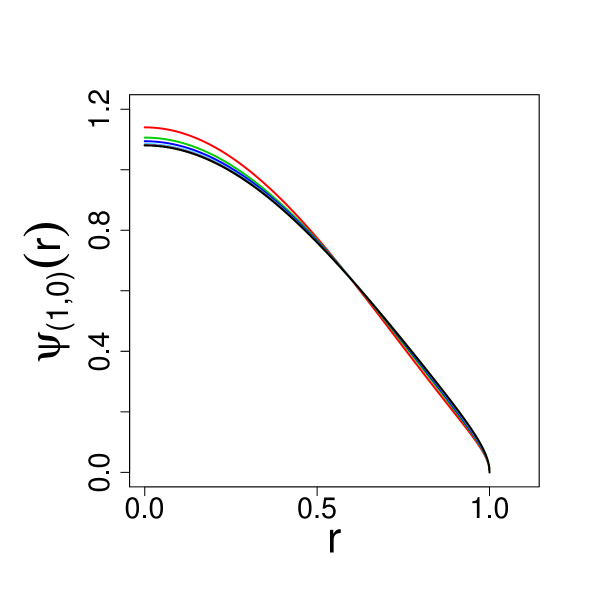
Figure 1: A comparative display of approximate ground state functions $\psi_{(1,0)}^{(2n)}(r)$ for polynomial (approximation) degrees $2n=4,6,10,20,30,50,70,100,150,200,500$. For each consecutive curve, the maximum location drops down with the growth of $2n$. The $2n=500$ curve is depicted in black.

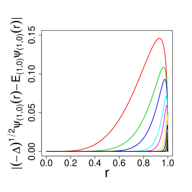
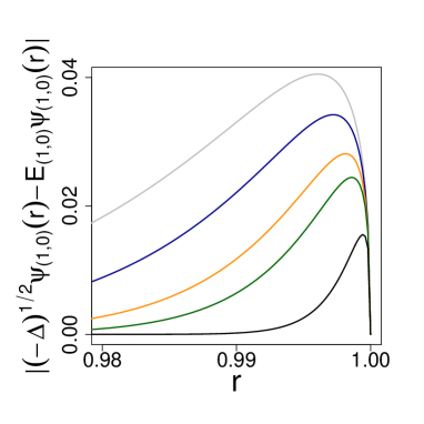
Figure 2: Detuning between the polynomial $(-\Delta)^{1/2}\psi^{(2n)}_{(1,0)}(r)$ of the degree $2n$ and the non-polynomial approximate expression $E^{(2n)}_{(1,0)}\psi^{(2n)}_{(1,0)}(r)$. Left panel: a comparative display for $2n=4,6,10,20,30,50,70,100,150,200,500$. Right panel: the detuning display for $2n=70,100,150,200,500$. The $2n=500$ curve is depicted in black.

Figure 3: Contour shapes of approximate purely radial eigenfunctions $\psi^{(500)}_{(k,0)}(r)$ for $k=2,3,4$.

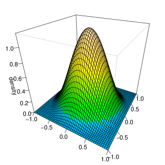
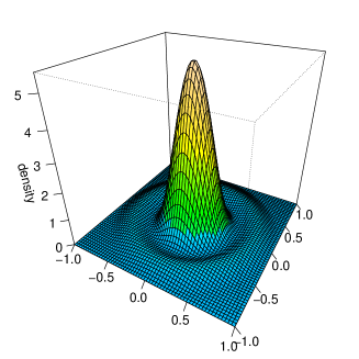
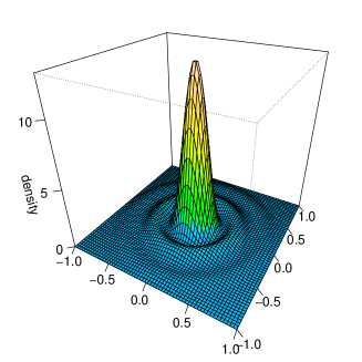
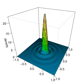
Figure 4: Comparative display of polar $(r,\theta)$ plots for probability densities $|\psi^{(500)}_{(k,0)}(r)|^{2}$ with $k=1,2,3,4$. Note scale changes along the vertical (density values) axis, necessary to fit the location of maxima.

We have explicitly computed solution values of $E^{(2n)}$ and $C^{(2n)}$, together with all expansion coefficients $\alpha^{(2n)}_{2k},k=1,...,n$ for each polynomial $w_{2n}$ appearing as a building block of an approximate ground state function $\psi^{(2n)}(r)=C^{(2n)}\sqrt{1-r^{2}}w_{2n}(r)$. In Table I, we have displayed selected coefficients only. The convergence properties of the data associated with $\psi_{2n}$, as $n$ approaches $250$, set a solid ground for further computational analysis of excited states.

The data displayed in Table I clearly demonstrate that the approximate ground state eigenvalue $E^{(2n)}$ drops down, showing a distinctive stabilization tendency. Our computed (approximate) ground state eigenvalue $E^{(500)}=2.754769$, up to the fifth decimal digit coincides with the value obtained independently in D (see e.g. Table 4 on page 552).

Since we have in hands all coefficients $\alpha^{(2n)}_{2k},k\geq n$ (not displayed in the present paper), that determine consecutive polynomials $w_{2n}$ from n=1 up to $n=250$, it is possible to make a comparative display of various curves $\psi^{(2n)}(r)$ with $n\leq 250$. The data in Fig. 1 show convincingly how close to the true (limiting) ground state of the (ultrarelativistic) infinite spherical well we actually are, even for relatively small values of $n$.

In Fig. 1 we employ the notation $\psi_{(1,0)}(r)$ for the ground state function and its approximations. We tentatively mention that the $2l+1$-fold ($|m|\leq l$) degeneracy of eigenvalues in each $l>0$ spectral series will enforce the usage of the third index $m$. We anticipate as well the splitting of the spherical well spectrum into the family of independent $l=0,1,2,...$ eigenvalue series $E_{(k,l)}$, $k=1,2,3,...$.

We have displayed curves $\psi^{(2n)}_{(1,0)}(r)$ for $2n=4,6,10,20,30,50,70,100,150,200,500$. The best approximation ($2n=500$) of the ground state function is depicted in black. We point out that maxima of approximating curves consecutively drop down with the growth of $n$.

All coefficients $\alpha_{2k},k\leq n$, together with $E^{(2n)}$, were explicitly computed after completing a severe truncation of the resultant polynomial expressions on both sides of the identity (26), down to the degree $2n$. Accordingly, the right-hand-side of (26) seems to have not much in common with $E^{(2n)}\,\psi^{(2n)}(r)$, where merely $w_{2n}(r)$ factor obeys the truncation restriction, while $\sqrt{1-r^{2}}$ remains untouched (is not truncated at all). That is not so.

In Fig. 2, for each value of $2n=4,6,10,20,30,50,70,100,150,200,500$, we compare directly the computed polynomial expression of the $2n$-th degree $(-\Delta)^{1/2}\psi^{(2n)}(r)$ with the complete (openly non-polynomial) expression $E^{(2n)}\,\psi^{(2n)}(r)=E^{(2n)}C^{(2n)}\sqrt{1-r^{2}}w_{2n}(r)$. That is accomplished by means of the point-wise detuning measure $|(-\Delta)^{1/2}\psi^{(2n)}(r)-E^{(2n)}\,\psi^{(2n)}(r)|$ which quantifies a difference (actually its modulus) between the two pertinent expressions.

The detuning proves to be fairly small ($<0.017$ for $2n=500$), remains sharply concentrated in a close vicinity of the $r=1$ boundary (negligible for $r<0.993$), and quickly decays to $0$ with the growth of $n$. In Fig, 2 we have displayed a convincing graphical proof of both the reliability of our approximation method and of the conspicuous convergence (in fact that of the detuning) of $\psi^{(2n)}(r)$ towards an ultimate ground state $\psi_{(1,0)}(r)$, as $n\rightarrow\infty$.

III.3 $l=0$ series.

We point out that the system of equations (31) allows to deduce approximate radial forms of higher eigenfunctions and eigenvalues in the infinite spherical well problem. Clearly, there are many other solutions available (including the complex ones, which we discard). After selecting the lowest eigenvalue $E=E_{(1,0)}$ (associated with the ground state $\psi_{(1,0)}(r)$), in the increasingly ordered set of $E$’s, we select the least one with the property $E_{(2,0)}<E_{(3,0)}$.

The approximate value of $E^{(2n)}_{(2,0)}$ for the $2n=500$-th excited state

$$\psi^{(2n)}_{(2,0)}(r,\phi,\theta)=C^{(2n)}\sqrt{1-r^{2}}\sum_{k=0}^{n}\alpha_{2k}r^{2k},\qquad\alpha_{0}=1$$ (31)

reads $E_{(2,0)}^{(500)}=5.8922138$.

Obviously, in the course of the computation (according to (30)) we have recovered not only the approximate eigenvalue, but the approximate eigenfunction as well. We recall that expansion coefficients $\alpha_{2k}$ with $k\leq 250$ come out as solutions of Eq. (31) together with the value of $E^{(2k)}$. We do not reproduce the detailed computation data (available upon request), we also abstain from presenting the detuning estimates. Results are similar to those obtained for the ground state function.

Selecting other solutions of Eq. (30) associated with with consecutive eigenvalues in an increasing sequence $E_{(1,0)}<E_{(2,0)}<E_{(3,0)}<...$ we are able to deduce the functional forms $\psi_{(k,0)}^{(2n)}(r)$ of higher (approximate) excited eigenfunctions of the purely radial form. These eigenvalues correspond to other purely radial solutions $\psi^{(2n)}_{(k,0)}(r)$, $k=2,3,4$ of Eqs. (30).

In Fig. 3 we depict the (contour) shapes of lowest radial eigenfunctions, while in Fig. 4 polar $(r,\theta)$ diagrams of related probability densities, with the $z$-axis directed perpendicular and inwards, relative to the picture frame.

III.4 Link between $d=1$ and $d=3$ infinite well ($l=0$) spectral series.

$E_{(k,0)}(d=3)=E_{2k}(d=1)$	1	2	3	4	5	6
2n=500	2.754769	5.892214	9.033009	12.174403	15.316005	18.457716
Ref. KGSZ	2.754795	5.892233	9.032984	12.174295	15.315777	18.457329
Ref. K	2.748894	5.890486	9.032079	12.173672	15.315554	*

Table 2: A comparison of approximate eigenvalues $E_{(k,0)}$ of the infinite spherical Cauchy well with approximate eigenvalues $E_{2k}$ of the $d=1$ infinite Cauchy well, as reported in KGSZ ; K .

For a particular choice $2n=500$ of the polynomial $w_{(2n)}$ degree, we have computed few lowest eigenvalues. They read: $E^{(500)}_{(2,0)}=5.892214$, $E^{(500)}_{(3,0)}=9.033009$ and $E^{(500)}_{(4,0)}=12.174403$. Interestingly, the obtained $d=3$ eigenvalues, at least up to five decimal digits, coincide with independently derived even-labelled eigenvalues $E_{2},E_{4},E_{6},E_{8}$ of the $d=1$ infinite Cauchy well spectral problem, ZG ; KGSZ .

In Table II we have collected comparatively the pertinent computed $d=3$ eigenvalues $E_{(k,0)}$ with $d=1$ results taken from KGSZ ; K . We point out that eigenvalues computed in K and KGSZ originally were set against the (asymptotically valid in $d=1$) formula $E_{k}\sim k\pi/2-\pi/8$, where $k\in 2\mathbb{N}$.

We note that the computation fidelity of higher eigenvalues is quite sensitive on the sufficiently large degree $2n$ of the polynomial approximation involved. Accordingly, we need very large $2n$ to infer a reliable approximation of $E_{(k,0)}$ if $k=100$ for example.

We hereby identify the generic feature of the spectrum of the Cauchy spherical well, that a subset $E_{(k,0)}$ of all $l=0$ eigenvalues is identical with that of even labeled eigenvalues of the $d=1$ Cauchy well: $E_{(k,0)}(d=3)=E_{2k}(d=1)$. Its asymptotic (large $k$) behavior is controlled by the $d=1$ formula, K ; KKMS ; ZG

$$E_{2k}\sim k\pi-\pi/8.$$ (32)

In the literature we have found some hints in this connection, D ; DKK , but the above conjecture has never been spelled out. The pertinent discussion has been focused on relating the ground state eigenvalue of the Cauchy well in $d>2$ with a suitable lower dimensional even-labeled eigenvalue.

Indeed, our computed ground state eigenvalue appears to coincide (fapp - for all practical purposes) with the first excited state eigenvalue of the $d=1$ Cauchy well, c.f. ZG ; KGSZ . This observation finds support in earlier theoretical results D . Namely, if $E_{*}$ is the lowest eigenvalue for which there exists the odd eigenfunction in the $d$-dimensional space, $E_{*}$ coincides with the eigenvalue of the radial ground state in the $(d+2)$ - dimensional space. This observation holds true for any $d$ (cf. Theorem 2 in Ref. D ).

Let us notice that in accordance with our analysis of the $d=3$ case, polynomial expansion coefficients of the ground state function are identical with $d=1$ polynomial coefficients of the first excited state. To this end one should simply compare Eqs. (58)-(62) of Ref. ZG with our present formulas (26)-(31). Indeed, we have:

$$\begin{array}[]{ccc}\psi_{2}(x)=C\sqrt{1-x^{2}}\sum\limits_{n=0}^{\infty}\beta_{2n+1}x^{2n+1},&&\psi_{(1,0)}(r)=C\sqrt{1-r^{2}}\sum\limits_{n=0}^{\infty}\alpha_{2n}r^{2n},\\ d=1,&&d=3,\end{array}$$ (33)

and clearly $\beta_{2n+1}=\alpha_{2n}$, for any $n\in\mathbb{N}$. Because other radial solutions (excited states) come out the same way from (30), our ($d=3$ versus $d=1$) conjecture seems to be unquestionably valid.

Remark 1: This peculiar interplay between $d=1$ and $d=3$ spectral data may justified directly by investigating the properties of respective Cauchy operators. Let $|z|\neq 0$. Assuming that we deal with the purely radial $d=3$ eigenfunction we have

$$\left((-\Delta)^{1/2}\psi(x,y,z)\right)(0,0,|z|)=\left(I_{1}-I_{2}\right)=E\psi(|z|),$$

where

$$I_{1}=\frac{1}{\pi^{2}}\left(\int\limits_{0}^{\infty}dr\int\limits_{0}^{2\pi}d\phi\int\limits_{0}^{\pi}d\theta\frac{\psi(|z|)r^{2}\sin\theta}{(r^{2}-2r|z|\cos\theta+|z|^{2})^{2}}\right)=\frac{\psi(|z|)}{\pi|z|}\int\limits_{0}^{\infty}r\left(\frac{1}{(r-|z|)^{2}}-\frac{1}{(r+|z|)^{2}}\right)dr,$$

and

$$I_{2}=\frac{1}{\pi^{2}}\left(\int\limits_{0}^{1}dr\int\limits_{0}^{2\pi}d\phi\int\limits_{0}^{\pi}d\theta\frac{\psi(r)r^{2}\sin\theta}{(r^{2}-2r|z|\cos\theta+|z|^{2})^{2}}\right)=\frac{1}{\pi|z|}\int\limits_{0}^{1}r\psi(r)\left(\frac{1}{(r-|z|)^{2}}-\frac{1}{(r+|z|)^{2}}\right)dr.$$

Let us assume that actually $\psi(r)$ is an even function i.e. $\psi(r)=\psi(-r)$. Then, presuming $0<z<1$ we can make a formal change of the integration variable $r\rightarrow-r$ in the second integrand (and related integral). We get:

$$I_{1}=\frac{\psi(z)}{\pi z}\int\limits_{-\infty}^{\infty}\frac{r}{(r-z)^{2}}dr,$$

and accordingly ($r$ is interpreted to belong to the integration interval $[-1,1]$)

$$I_{2}=\frac{1}{\pi z}\int\limits_{-1}^{1}\frac{r\psi(r)}{(r-z)^{2}}dr.$$

Presuming $-1<z<0$ we get similar results (except that we make a change of the integration variable $r\rightarrow-r$ in the first integrand). That extends the validity of the previous two identities (for $I_{1}$ and $I_{2}$) to any $z\in(-1,0)\cup(0,1)$.
Remembering that all integrations are carried out in the sense of the Cauchy principal values, we have also:

$$\int\limits_{-\infty}^{\infty}\frac{r}{(r-z)^{2}}dr=\int\limits_{-\infty}^{\infty}\frac{(r-z)+z}{(r-z)^{2}}dr=\int\limits_{-\infty}^{\infty}\frac{z}{(r-z)^{2}}dr.$$

Accordingly there holds

$$\frac{1}{\pi}\left(\int\limits_{-\infty}^{\infty}\frac{z\psi(z)}{(r-z)^{2}}-\int\limits_{-1}^{1}\frac{r\psi(r)}{(r-z)^{2}}dr\right)=Ez\psi(z),$$

to be compared with Eq. (4), originally defining the eigenvalue problem for the $d=1$ Cauchy operator.

An immediate conclusion follows. If an even (purely radial) function $\psi(z)$ is a solution of the $d=3$ eigenvalue problem, then the odd function $z\psi(z)$ actually is a solution of the $d=1$ eigenvalue problem. Surely an odd function cannot be a ground state, but an excited state of the $d=1$ spectral problem.
The above reasoning can be inverted and thence by departing from the odd $d=1$ eigenfunction 1D ($z\psi(z)$, (where clearly $\psi(z)$ is even) we end up with $\psi(z)$ as a legitimate eigenfunction of the $d=3$ spectral problem. Moreover, both functions share the same eigenvalue.

Remark 2: In Ref. ZG we have proposed an analytic expression for the approximate excited eigenfunction of the $d=1$ infinite Cauchy well:

$$\psi_{2}(x)=-C\sin(\beta x)\sqrt{(1-x^{2})\cos(\beta x)},$$ (34)

where C=1.99693 is a normalization constant in $d=1$, while the parameter $\beta$ has been optimized to take the value $\beta=1760\pi/4096$. Our discussion in the previous Remark 1, sets a transparent link between the first excited state in $d=1$ and the ground state in $d=3$. Let us introduce

$$\psi(r)=C\frac{\sin(\beta r)\sqrt{(1-r^{2})\cos(\beta r)}}{r},\qquad r=\sqrt{x^{2}+y^{2}+z^{2}}$$ (35)

as an admissible analytic expression for the ”natural” approximation of the ground state in $d=3$. Here, the normalization constant needs to be evaluated in $d=3$ and equals (with an accuracy up to six decimal digits) $C=0.796658$.

In Fig. 5 we display comparatively the $d=3$ analytic curve (red) (35) against the approximate ground state $\psi_{(1,0)}^{(500)}$ (black). An agreement is striking. For more detailed discussion of the $d=1$ case, see e.g. Section II.D in Ref. ZG .

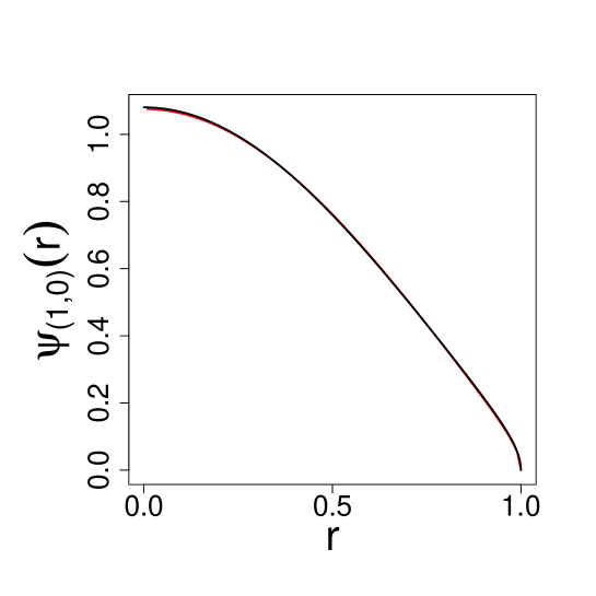
Figure 5: Comparative display of two approximations of the ground state in $d=3$, the analytic form (in red) and $\psi_{(1,0)}^{(500)}$, see e.g. Fig. 1 (in black). The maximum of the analytic curve (red) is residually shifted down if compared with the computed (black) approximate outcome.

Remark 3: The previously discussed $d=1$ versus $d=3$ interplay of Cauchy well spectral problems has its close analog in standard quantum mechanics, where the minus Laplacian replaces our fractional operator). Let us consider the $d=1$ symmetric infinite well on the open set $(-1,1)$. For all $x\in(-1,1)$ we have the Schrödinger eigenvalue problem (we set $m=\hbar=1$) in the form

$$-\frac{1}{2}\frac{\partial^{2}\psi}{\partial x^{2}}=E\psi$$

Its solutions have the standard form: $\psi^{p}_{n}(x)=C\cos[(\pi/2+n\pi)x]$, $E^{p}_{n}=(\pi/2+n\pi)^{2}/2$, $n\in\mathbb{N}$ (even, i.e. $n=2k$) and $\psi^{n}_{n}(x)=C\sin(n\pi x)$, $E^{n}_{n}=(n\pi)^{2}/2$, $n\in\mathbb{N}_{+}$ (odd, $n=2k+1$). Energy eigenvalues, in the notation encompassing both families of eigenfunctions, read: $E_{n}=n^{2}\pi^{2}/8$, where $n\in\mathbb{N}_{+}$. The ground state energy $E_{1}=\pi^{2}/8$ corresponds to the even function, while the first odd one $C\sin(\pi x)$ refers to the excited state with $E_{2}=\pi^{2}/2$.
The radial part of the $d=3$ Schrödinger equation for $l=0$ takes the form

$$-\frac{1}{2}\frac{\partial^{2}R}{\partial r^{2}}-\frac{1}{r}\frac{\partial R}{\partial r}=ER.$$

Both $\cos(\gamma_{2n+1}r)/r$ and $\sin(\gamma_{2n}r)/r$, where $\gamma_{n}=n\pi/2$, are solutions of this equation. However the blow-up property of $\cos(\gamma_{2n+1}r)/r$ as $r\to 0$ enforces discarding of that function from the analysis. Accordingly, solutions of the radial equation have the form $\sin(\gamma_{2n}r)/r$. Clearly $\sin(\pi r)/r$ (up to normalization) stands for the ground state with the eigenvalue $E=\pi^{2}/2$.
In passing, we point out G , that other eigenfunctions for the $d=3$ infinite spherical well can be deduced by addressing the fully-fledged eigenvalue problem with $l\neq 0$. Eigensolutions are given in terms of Bessel functions and energy values read $E_{kl}=(u_{l,k}^{2}/2)$, where $u_{l,k}$ are the Bessel function zeroes. For each choice of $l=0,1,2,...$ we recover the $l$-th eigenvalue series labelled by $k=1,2,...$. It is worthwhile to mention that for large $k$, the series look quite regular, in view of $u_{l,k}\sim\pi(k+{\frac{l}{2}})$. In particular, one can prove that for $l=0$ the Bessel function takes the form $j_{0}(r)=\sin(r)/r$ which clearly has zeroes at $k\pi$. The corresponding eigenvalues read $E_{k0}=(k\pi)^{2}/2$, $k\in\mathbb{N}_{+}$ and form the $l=0$-series of eigenvalues.

IV Orbitally nontrivial eigenstates, $l\geq 1$ series.

IV.1 Prerequisites.

In the previous section we have relied on some $d=1$ intuitions in computing the ground state data for the infnite spherical well. We find them useful in the search for non-radial eigenfunctions, albeit after some preliminary discussion on how the rotational symmetry of the problem may help in making computations easier.

Let us specify a point $P$ as the endpoint of the vector $OP=\textbf{p}=(x_{1},x_{2},x_{3})\in D$. By executing a suitable three dimensional rotation, we may pass to a new coordinate system whose $Oz$ axis contains $P$. Clearly, for such $P$, the identity $x_{1}^{2}+x_{2}^{2}=0$ would imply $x_{1}=x_{2}=0$. Consistently, we may safely assume $x_{1}^{2}+x_{2}^{2}\neq 0$ to hold true in general.

Our further considerations critically rely on a proper change (rotation) of the reference frame in $\mathbb{R}^{3}$, under the assumption made. The pertinent frame of reference change would result in the rotation of coordinates

$$y=R_{y}R_{z}x=\left(0,0,\sqrt{x_{1}^{2}+x_{2}^{2}+x_{3}^{2}}\right)^{T},$$ (36)

where we denote $y=(y_{1},y_{2},y_{3})^{T}$, $x=(x_{1},x_{2},x_{3})^{T}$, ($T$ indicates that the vector is transposed) while $R_{x}$ and $R_{y}$ are rotation matrices around $OY$ and $OZ$ respectively. They read:

$$R_{z}=\left(\begin{array}[]{ccc}\cos\phi&\sin\phi&0\\ -\sin\phi&\cos\phi&0\\ 0&0&1\\ \end{array}\right),$$ (37)

$$R_{y}=\left(\begin{array}[]{ccc}\cos\theta&0&-\sin\theta\\ 0&1&0\\ \sin\theta&0&\cos\theta\\ \end{array}\right),$$ (38)

where

$$\cos\phi=\frac{x_{1}}{\sqrt{x_{1}^{2}+x_{2}^{2}}},\qquad\sin\phi=\frac{x_{2}}{\sqrt{x_{1}^{2}+x_{2}^{2}}},$$ (39)

$$\cos\theta=\frac{x_{3}}{\sqrt{x_{1}^{2}+x_{2}^{2}+x_{3}^{2}}},\qquad\sin\theta=\frac{\sqrt{x_{1}^{2}+x_{2}^{2}}}{\sqrt{x_{1}^{2}+x_{2}^{2}+x_{3}^{2}}}.$$ (40)

Clearly, the inverse rotation matrix gives rise to $x=R^{-1}_{z}R^{-1}_{y}y$. We denote $S=R^{-1}_{z}R^{-1}_{y}$. Its explicit form is

$$S=\left(\begin{array}[]{ccc}\frac{x_{1}x_{3}}{\sqrt{x_{1}^{2}+x_{2}^{2}}\sqrt{x_{1}^{2}+x_{2}^{2}+x_{3}^{2}}}&-\frac{x_{2}}{\sqrt{x_{1}^{2}+x_{2}^{2}}}&\frac{x_{1}}{\sqrt{x_{1}^{2}+x_{2}^{2}+x_{3}^{2}}}\\ \frac{x_{2}x_{3}}{\sqrt{x_{1}^{2}+x_{2}^{2}}\sqrt{x_{1}^{2}+x_{2}^{2}+x_{3}^{2}}}&\frac{x_{1}}{\sqrt{x_{1}^{2}+x_{2}^{2}}}&\frac{x_{2}}{\sqrt{x_{1}^{2}+x_{2}^{2}+x_{3}^{2}}}\\ -\frac{\sqrt{x_{1}^{2}+x_{2}^{2}}}{\sqrt{x_{1}^{2}+x_{2}^{2}+x_{3}^{2}}}&0&\frac{x_{3}}{\sqrt{x_{1}^{2}+x_{2}^{2}+x_{3}^{2}}}\\ \end{array}\right).$$ (41)

In Section II we have given $d=3$ Cauchy operator a somewhat formal but computationally convenient integral form $I_{1}-I_{2}$ (remember about our precautions concerning the close neighborhood of $(0,0,0)$). We have:

$$(-\Delta)^{1/2}\psi(x_{1},x_{2},x_{3})=$$ (42)

$$\frac{1}{\pi^{2}}\left(\int\limits_{\mathbb{R}^{3}}\frac{\psi(x_{1},x_{2},x_{3})du}{((u_{1}-x_{1})^{2}+(u_{2}-x_{2})^{2}+(u_{3}-x_{3})^{2})^{2}}-\int\limits_{D}\frac{\psi(u_{1},u_{2},u_{3})du}{((u_{1}-x_{1})^{2}+(u_{2}-x_{2})^{2}+(u_{3}-x_{3})^{2})^{2}}\right),$$

where $du=du_{1}du_{2}du_{3}$.

The integration procedure will be carried out as follows. We execute an inverse rotation of $u$ according to the previous recipe, e.g. $u=Sv$ and employ $x=Sy$ where $y=\left(0,0,\sqrt{x_{1}^{2}+x_{2}^{2}+x_{3}^{2}}\right)^{T}$. We note the $D$ is rotation invariant (spherical well) and the modulus of the Jacobian of the transformation $S$ equals $1$. Substituting

$$u_{i}=s_{i1}v_{1}+s_{i2}v_{2}+s_{i3}v_{3},\qquad i=1,2,3,$$ (43)

where $s_{ij}$ are matrix elements of $S$ we get

$$\sqrt{u_{1}^{2}+u_{2}^{2}+u_{3}^{2}}\xrightarrow{S}\sqrt{v_{1}^{2}+v_{2}^{2}+v_{3}^{2}},$$ (44)

$$(u_{1}-x_{1})^{2}+(u_{2}-x_{2})^{2}+(u_{3}-x_{3})^{2}\xrightarrow{S}v_{1}^{2}+v_{2}^{2}+\left(v_{3}-\sqrt{x_{1}^{2}+x_{2}^{2}+x_{3}^{2}}\right)^{2}.$$ (45)

That is the starting point for our further analysis.

IV.2 $l=1$ series.

We denote $\textbf{p}=(x_{1},x_{2},x_{3})$ and $p=\sqrt{x_{1}^{2}+x_{2}^{2}+x_{3}^{2}}$. Our next assumption pertains to the anticipated functional form of the excited eigenstate with an orbital (angular) input, i.e. being non-radial. We make a trial ansatz (note the a priori insertion of orbital labels, to be justified in below):

$$\psi_{(1,1,0)}(\textbf{p})=C\,x_{3}\,f(p),$$ (47)

$$f(p)=\sqrt{1-p^{2}}\sum\limits_{k=0}^{\infty}\beta_{2k}p^{2k},$$

where $C$ is the normalization factor. We assume furthermore that $\beta_{0}=1$.

We shall demonstrate that Eq. (47) indeed determines a proper functional form of the first excited eigenfunction and entails a computation of its fairly accurate approximations. Like in Section II, we shall execute integrations of the series expansion in (47) term after term.

First we shall prove that:

$$(-\Delta)^{1/2}\left(u_{3}\sqrt{1-(u_{1}^{2}+u_{2}^{2}+u_{3}^{2})}\right)(\textbf{p})=\frac{8}{3}x_{3}.$$ (48)

We need to evaluate (while taking care of divergent contributions two integral expressions $I_{1}(\textbf{p})$ and $I_{2}(\textbf{p})$, before eventually subtracting them and so eliminating singular contributions. We have:

$$I_{1}(\textbf{p})=\frac{1}{\pi^{2}}\int\limits_{\mathbb{R}^{3}}\frac{x_{3}\sqrt{1-(x_{1}^{2}+x_{2}^{2}+x_{3}^{2})}}{((u_{1}-x_{1})^{2}+(u_{2}-x_{2})^{2}+(u_{3}-x_{3})^{2})^{2}}du=\frac{x_{3}\sqrt{1-p^{2}}}{\pi^{2}}\int\limits_{\mathbb{R}^{3}}\frac{dv}{(v_{1}^{2}+v_{2}^{2}+(v_{3}-p)^{2})^{2}}.$$ (49)

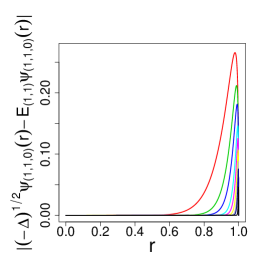
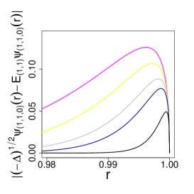
Figure 6: Left panel: contour plot of $\psi^{(500)}_{(1,1,0)}$ for $\theta=0$. Middle panel: Comparative display of detuning curves for $\psi_{(1,1,0)}$ at $\theta=0$, polynomial approximations of degrees $10,20,30,50,70,100,150,200,500$. The maximum drops down with the growth of $2n$. The optimal (2n=500) curve is depicted in black. Right panel: detuning for polynomial approximations of degrees $70,100,150,200,500$.

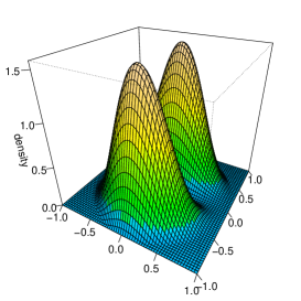
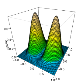
Figure 7: Probability densities $|\psi^{(500)}_{(1,1,0)}(r,\phi,\theta)|^{2}$ (left) and $|\psi^{(500)}_{(1,1,\pm 1)}(r,\phi,\theta)|^{2}$ (right) in polar coordinates.

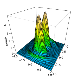
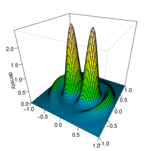
Figure 8: Contour plot of $\psi^{(500)}_{(2,1,0)}$ at $\theta=0$ (left). Probability densities $|\psi^{(500)}_{(2,1,0)}(r,\phi,\theta)|^{2}$ (midddle) and $|\psi^{(500)}_{(2,1,\pm 1)}(r,\phi,\theta)|^{2}$ (right) in polar coordinates.

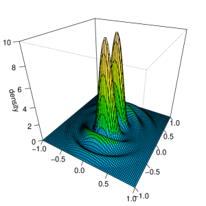
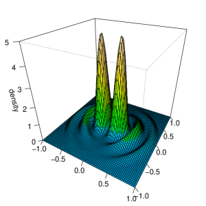
Figure 9: Contour plot of $\psi^{(500)}_{(3,1,0)}$ at $\theta=0$. Probability densities $|\psi^{(500)}_{(3,1,0)}(r,\phi,\theta)|^{2}$ (middle) and $|\psi^{(500)}_{(3,1,\pm 1)}(r,\phi,\theta)|^{2}$ in polar coordinates.

After passing to spherical coordinates we get

$$I_{1}(\textbf{p})=\frac{x_{3}\sqrt{1-p^{2}}}{\pi^{2}}\int\limits_{0}^{\infty}dr\int\limits_{0}^{2\pi}d\phi\int\limits_{0}^{\pi}d\theta\frac{r^{2}\sin\theta}{(r^{2}-2rp\cos\theta+p^{2})^{2}}=\frac{2x_{3}\sqrt{1-p^{2}}}{\pi}\lim\limits_{\varepsilon\to 0}\frac{1}{\varepsilon}.$$ (50)

The integral entry $I_{2}(\textbf{p})$ reads

$$I_{2}(\textbf{p})=\frac{1}{\pi^{2}}\int\limits_{D}\frac{u_{3}\sqrt{1-(u_{1}^{2}+u_{2}^{2}+u_{3}^{2})}}{((u_{1}-x_{1})^{2}+(u_{2}-x_{2})^{2}+(u_{3}-x_{3})^{2})^{2}}du=\frac{1}{\pi^{2}}\int\limits_{D}\frac{(s_{31}v_{1}+s_{32}v_{2}+s_{33}v_{3})\sqrt{1-(v_{1}^{2}+v_{2}^{2}+v_{3}^{2})}}{(v_{1}^{2}+v_{2}^{2}+(v_{3}-\sqrt{x_{1}^{2}+x_{2}^{2}+x_{3}^{2}})^{2})^{2}}dv,$$ (51)

We denote $v=\sqrt{v_{1}^{2}+v_{2}^{2}+v_{3}^{2}}$. The outcome of the $\phi$-integration in the range $[0,2\pi]$ is

$$\int\limits_{D}\frac{v_{1}\sqrt{1-v^{2}}}{(v_{1}^{2}+v_{2}^{2}+(v_{3}-p)^{2})^{2}}dv=\int\limits_{0}^{1}dr\int\limits_{0}^{2\pi}d\phi\int\limits_{0}^{\pi}d\theta\frac{r^{2}\sin\theta\cdot r\cos\phi\sin\theta\sqrt{1-r^{2}}}{(r^{2}-2rp\cos\theta+p^{2})^{2}}=0,$$ (52)

and quite analogously

$$\int\limits_{D}\frac{v_{2}\sqrt{1-v^{2}}}{(v_{1}^{2}+v_{2}^{2}+(v_{3}-\sqrt{x_{1}^{2}+x_{2}^{2}+x_{3}^{2}})^{2})^{2}}dv=0.$$ (53)

Accordingly:

$$I_{2}(\textbf{p})=\frac{s_{33}}{\pi^{2}}\int\limits_{D}\frac{v_{3}\sqrt{1-v^{2}}}{(v_{1}^{2}+v_{2}^{2}+(v_{3}-\sqrt{x_{1}^{2}+x_{2}^{2}+x_{3}^{2}})^{2})^{2}}dv=\frac{s_{33}}{\pi^{2}}\int\limits_{0}^{1}dr\int\limits_{0}^{2\pi}d\phi\int\limits_{0}^{\pi}d\theta\frac{r^{2}\sin\theta\cdot r\cos\theta\sqrt{1-r^{2}}}{(r^{2}-2rp\cos\theta+p^{2})^{2}}.$$ (54)

To evaluate (48) few more steps are necessary. Let us notice that

$$I_{2}(\textbf{p})={\frac{s_{33}}{2\pi p^{2}}}(I_{21}+I_{22}),$$ (55)

where

$$I_{21}=\int\limits_{0}^{1}r(r^{2}+p^{2})\sqrt{1-r^{2}}\left(\frac{1}{(r-p)^{2}}-\frac{1}{(r+p)^{2}}\right)dr,$$ (56)

$$I_{22}=\int\limits_{0}^{1}r\sqrt{1-r^{2}}\left(\ln(r-p)^{2}-\ln(r+p)^{2}\right)dr.$$ (57)

One may check the validity of the following indefinite integrals, GR :

$$\int\frac{r(r^{2}+p^{2})\sqrt{1-r^{2}}}{(r\mp p)^{2}}dr=\frac{\sqrt{1-r^{2}}(r^{3}\pm p\pm 2r^{2}p\mp 18p^{3}+r(-1+9p^{2}))}{3(r\mp p)}\pm p(1-6p^{2})\arcsin(r)$$

$$-\frac{2p^{2}(-2+3p^{2})\ln\left|r\mp p\right|}{\sqrt{1-p^{2}}}+\frac{2p^{2}(-2+3p^{2})\ln(1\mp rp+\sqrt{1-r^{2}}\sqrt{1-p^{2}})}{\sqrt{1-p^{2}}},$$ (58)

and

$$\int r\sqrt{1-r^{2}}\ln(r\mp p)^{2}\,dr=\frac{1}{3}\left[\frac{1}{3}\sqrt{1-r^{2}}\left(8-2r^{2}\mp 3rp-6p^{2}\right)\pm p(-3+2p^{2})\arcsin(r)\right.$$

$$\left.+2(1-p^{2})^{3/2}\ln\left|r\mp p\right|-(1-r^{2})^{3/2}\ln(r\mp p)^{2}-2(1-p^{2})^{3/2}\ln(1\mp rp+\sqrt{1-r^{2}}\sqrt{1-p^{2}})\right].$$ (59)

Remembering about our precautions concerning singular terms and employing $s_{33}p=x_{3}$, we ultimately arrive at

$$I_{2}=-\frac{8}{3}x_{3}+\frac{x_{3}}{\pi}\lim\limits_{\varepsilon\to 0}\left(\frac{\sqrt{1-(p-\varepsilon)^{2}}}{\varepsilon}+\frac{\sqrt{1-(p+\varepsilon)^{2}}}{\varepsilon}\right).$$ (60)

While subtracting formal expressions we note that all divergent terms cancel each other and consistently there holds

$$I_{1}-I_{2}=\frac{8}{3}x_{3},$$ (61)

as anticipated.

Let $u=\sqrt{u_{1}^{2}+u_{2}^{2}+u_{3}^{2}}$. Analogously, albeit somewhat tediously, we handle subsequent expansion terms in our formula (47), with an outcome valid for all $n$:

$$(-\Delta)^{1/2}\left(u_{3}u^{2n}\sqrt{1-u^{2}}\right)(x_{1},x_{2},x_{3})=\left(4x_{3}\sum\limits_{k=0}^{n}c_{2k}\frac{(n+1-k)(n+2-k)}{(2n+3-2k)}p^{2n-2k}\right),$$ (62)

where $c_{2k}$ are coefficients of the Taylor expansion of $\sqrt{1-z^{2}}$, c.f. also Section II.

Upon inserting the trial function (47) to the eigenvalue equation (5), we arrive at (c.f. also Section II.B and note that the resultant identity needs to hold true for all $x_{3}=p\cos\theta$):

$$\sum_{k=0}^{\infty}\sum_{n=k}^{\infty}\beta_{2n}b_{k,n}p^{2n-2k}=\sum_{k=0}^{\infty}\sum_{n=0}^{\infty}E\beta_{2n}c_{2k}p^{2k+2n},$$ (63)

where

$$b_{k,n}=4\frac{(n+1-k)(n+2-k)}{(2n+3-2k)}c_{2k},$$ (64)

and we have

$$c_{2k}=\frac{(2k)!}{(1-2k)(k!)^{2}4^{k}}.$$ (65)

The analytic solution of the system of linear equations (63) is not in the reach. Therefore we reiterate to the very same truncation method (polynomial approximation) we have employed in Section II.B, and we follow steps (i)-(iii) there in.

The system of $2n+1$ equations for $2n+1$ unknowns $E$ and $\beta_{2k}$ (we recall that $\beta_{0}=1$, by assumption), corresponding to the polynomial approximation of the degree $2n$, has the form

$$\sum\limits_{k=i}^{n}\beta_{2k}b_{k-i,k}=E\sum\limits_{k=0}^{i}\beta_{2k}c_{2(i-k)},\qquad i=0,1,\ldots,n-1,$$

$$\sum\limits_{m=0}^{n}\left(\beta_{2m}\sum\limits_{k=0}^{m}b_{k,m}\right)=0.$$ (66)

The last identity is an outcome of the boundary condition (iii) i.e. $(-\Delta)^{1/2}\psi_{(1,1,0)}(r,\phi,\theta)$ at the boundary $r=1$.

Wolfram Mathematica routines allow to handle large systems of linear equations of the form (66). The computation allows to recover both the approximate eigenfunction $\psi^{(500)}_{(1,1,0)}(r,\phi,\theta)$ and the corresponding eigenvalue $E^{(500)}_{(1,1)}=4.121332$. It is worthwhile to mention that in Table 4 of Ref. D the same eigenvalue has been independently computed with the outcome (notation of D ) $\lambda_{*}=4.12131$. The original motivation of Ref. D was to demonstrate that the pertinent $\lambda_{*}$ (first excited eigenvalue in $d=3$) is identical with the ground state eigenvalue of the spherical well problem in dimension $d+2=5$.

Analogous considerations allow to prove that three trial functions of the form

$$x_{1}f(p),\qquad x_{2}f(p),\qquad x_{3}f(p),$$ (67)

give rise to real (approximate) eigenfunctions of the spherical well problem, sharing the eigenvalue $E_{(1,1)}$ and the radial factor $f(p)$.

Remark 5: Computations involve respectively $x_{1}$ or $x_{2}$ instead of $x_{3}$ in the integral expression $I_{1}$. Evaluation of the integral expression $I_{2}$ would look similarly. However, the change of variables (appropriate rotation of the intrinsic coordinate system) would transform $u_{i}$ ($i=1,2$) to $s_{i1}v_{1}+s_{i2}v_{2}+s_{i3}v_{3}$. Integrals containing $v_{1}$ i $v_{2}$ would vanish identically. We note that in the ultimate formulas one deals with $s_{13}p=x_{1}$ and $s_{23}p=x_{2}$.

Consequently, in case of $l=1$ to the label $k=1$ there correspond three linearly independent real eigenfunctions with a common radial part $f(p)$. It is customary to pass to a complex system of eigenfunctions

$$\psi_{(1,1,0)}(\textbf{p})=Cx_{3}f(p)=C^{\prime}pY_{1}^{0}(\theta,\phi)f(p),$$ (68)

$$\psi_{(1,1-1)}(\textbf{p})=C(x_{1}-i\,x_{2})f(p)=C^{\prime}pY_{1}^{-1}(\theta,\phi)f(p),$$ (69)

$$\psi_{(1,1,1)}(\textbf{p})=C(x_{1}+i\,x_{2})f(p)=C^{\prime}pY_{1}^{1}(\theta,\phi)f(p),$$ (70)

where $\psi_{(1,1,m)}$, $m=-1,0,1$ can be given a familiar form of linear combinations of spherical harmonics (and solid harmonics in parallel), multiplied by the radial function $f(p)$, L ; Lei .

IV.3 $l=2$ series.

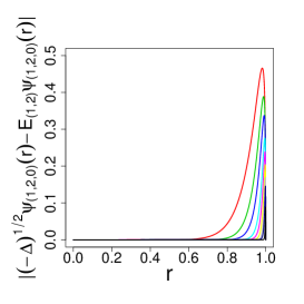
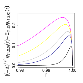
Figure 10: Contour plot of $\psi^{(500)}_{(1,2,0)}$ at $\theta=0$. The detuning for $\psi^{(500)}_{(1,2,0)}$ at $\theta=0$ for polynomial approximations with degrees $10,20,30,50,70,100,150,200,500$. The maximum drops down with the growth of $2n$. The $2n=500$ curve is depicted in black. Right: detuning for degrees $70,100,150,200,500$.

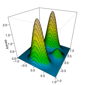
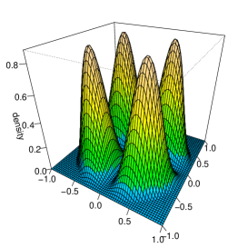
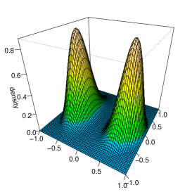
Figure 11: Probability densities in polar coordinates (from left to right): $|\psi^{(500)}_{(1,2,0)}(r,\phi,\theta)|^{2}$, $|\psi^{(500)}_{(1,2,\pm 1)}(r,\phi,\theta)|^{2}$ and $|\psi^{(500)}_{(1,2,\pm 2)}(r,\phi,\theta)|^{2}$ .

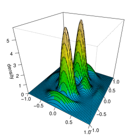
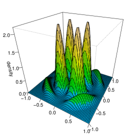
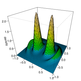
Figure 12: Probability densities (from left to right) $|\psi^{(500)}_{(2,2,0)}(r,\phi,\theta)|^{2}$, $|\psi^{(500)}_{(2,2,\pm 1)}(r,\phi,\theta)|^{2}$ and $|\psi^{(500)}_{(2,2,\pm 2)}(r,\phi,\theta)|^{2}$.

Our trial choice for the next ($k=1,l=2$, $m=0$ being anticipated) orbitally nontrivial bound state is

$$\psi_{(1,2,0)}(x_{1},x_{2},x_{3})=C\frac{3x_{3}^{2}-p^{2}}{2}f(p)$$ (72)

where

$$f(p)=\sqrt{1-p^{2}}\sum\limits_{k=0}^{\infty}\gamma_{2k}p^{2k},\qquad\gamma_{0}=1.$$ (73)

We follow the same methodology as before and skip detailed calculations. However, for the reader’s convenience we present an outline of main steps and reproduce the ultimate outcomes.

The integral expression $I_{1}$ takes the form

$$I_{1}=\frac{1}{\pi^{2}}\int\limits_{\mathbb{R}^{3}}\frac{3x_{3}^{2}-p^{2}}{2}\frac{\sqrt{1-p^{2}}}{((u_{1}-x_{1})^{2}+(u_{2}-x_{2})^{2}+(u_{3}-x_{3})^{2})^{2}}du=\frac{(3x_{3}^{2}-p^{2})}{\pi}\sqrt{1-p^{2}}\lim\limits_{\varepsilon\to 0}\frac{1}{\varepsilon},$$ (74)

while the evaluation of $I_{2}$ is more intricate. We have

$$I_{2}=\frac{1}{2\pi^{2}}\int\limits_{D}\frac{(3u_{3}^{2}-u^{2})\sqrt{1-u^{2}}}{((u_{1}-x_{1})^{2}+(u_{2}-x_{2})^{2}+(u_{3}-x_{3})^{2})^{2}}du=\frac{1}{2\pi^{2}}\int\limits_{D}\frac{[3(s_{31}v_{1}+s_{32}v_{2}+s_{33}v_{3})^{2}-v^{2}]\sqrt{1-v^{2}}}{(v_{1}^{2}+v_{2}^{2}+(v_{3}-p)^{2})^{2}}dv,$$ (75)

and a number of integrals need to be evaluated explicitly.

The final outcome is

$$(-\Delta)^{1/2}\left(\frac{3u_{3}^{2}-u^{2}}{2}\sqrt{1-u^{2}}\right)(x_{1},x_{2},x_{3})=\frac{16}{5}\left(\frac{3x_{3}^{2}-p^{2}}{2}\right)=\frac{1}{2}\left[3\left(4-\frac{1}{3}-\frac{1}{5}\right)-4\right]c_{0}\left(\frac{3x_{3}^{2}-p^{2}}{2}\right),$$ (76)

Analogously we arrive at

$$(-\Delta)^{1/2}\left(\frac{3u_{3}^{2}-u^{2}}{2}u^{2}\sqrt{1-u^{2}}\right)(x_{1},x_{2},x_{3})=\left(\frac{3x_{3}^{2}-p^{2}}{2}\right)\frac{1}{2}\left\{\left[3\left(4-\frac{1}{3}-\frac{1}{5}\right)-4\right]c_{2}+\left[3\left(6-\frac{1}{5}-\frac{1}{7}\right)-6\right]c_{0}p^{2}\right\},$$ (77)

$$\begin{split}(-\Delta)^{1/2}\left(\frac{3u_{3}^{2}-u^{2}}{2}u^{4}\sqrt{1-u^{2}}\right)(x_{1},x_{2},x_{3})&=\left(\frac{3x_{3}^{2}-p^{2}}{2}\right)\frac{1}{2}\left\{\left[3\left(4-\frac{1}{3}-\frac{1}{5}\right)-4\right]c_{4}\right.\\ &\left.+\left[3\left(6-\frac{1}{5}-\frac{1}{7}\right)-6\right]c_{2}p^{2}+\left[3\left(8-\frac{1}{7}-\frac{1}{9}\right)-8\right]c_{0}p^{4}\right\},\end{split}$$ (78)

where $c_{2k}$ are Taylor series expansion coefficients for $\sqrt{1-z^{2}}$. We note that

$$\frac{1}{2}\left[2(2n-2k+4)-3\left(\frac{1}{2n-2k+3}+\frac{1}{2n-2k+5}\right)\right]=\frac{8(n-k+1)(n-k+2)(n-k+3)}{(2n-2k+3)(2n-2k+5)},$$ (79)

hence, the general formula (referring to the $2n$-th power of $u$) takes the form

$$(-\Delta)^{1/2}\left(\frac{3u_{3}^{2}-u^{2}}{2}u^{2n}\sqrt{1-u^{2}}\right)(x_{1},x_{2},x_{3})=\left(\frac{3x_{3}^{2}-p^{2}}{2}\right)8\sum\limits_{k=0}^{n}\frac{(n-k+1)(n-k+2)(n-k+3)}{(2n-2k+3)(2n-2k+5)}c_{2k}p^{2n-2k}.$$ (80)

Upon inserting the trial function $\psi_{(1,2,0)}$ (Eqs. (72) and (73)) to the eigenvalue equation, we get

$$\sum_{k=0}^{\infty}\sum_{n=k}^{\infty}g_{k,n}\gamma_{2n}p^{2n-2k}=\sum_{k=0}^{\infty}\sum_{n=0}^{\infty}E\gamma_{2n}c_{2n}p^{2k+2n}.$$ (81)

where

$$g_{k,n}=c_{2n}\,\frac{8(n+1-k)(n+2-k)(n+3-k)}{(2n+3-2k)(2n+5-2k)}.$$ (82)

Like before, we have no tools to solve (81) analytically. Therefore we follow the approximation route of Section II.B, specifically steps (i) - (iii). The polynomial approximation of the degree $2n$ results in the linear system of $2n+1$ equations for unknowns $E$ and $\gamma_{2n}$ ($\gamma_{0}=1$ is presumed):

$$\sum\limits_{k=i}^{n}\gamma_{2k}g_{k-i,k}=E\sum\limits_{k=0}^{i}\gamma_{2k}c_{2(i-k)},\qquad i=0,1,\ldots,n-1,$$

$$\sum\limits_{m=0}^{n}\left(\gamma_{2m}\sum\limits_{k=0}^{m}g_{k,m}\right)=0.$$ (83)

The last identity is an outcome of the boundary condition (iii): $(-\Delta)^{1/2}\psi_{(1,2,0)}(r,\phi,\theta)$ at $r=1$.

The system is amenable to Wolfram Mathematica routines and allows to compute all $\gamma_{2k}$ and the (approximate) eigenvalue $E_{(1,2)}=5.400079$ associated with $\psi^{(500)}_{(1,2,0)}$. We can can demonstrate that five real functions:

$$(x_{1}^{2}-x_{2}^{2})f(p),\quad x_{1}x_{2}f(p),\quad x_{1}x_{3}f(p),\quad x_{2}x_{3}f(p),\quad(2x_{3}^{2}-x_{1}^{2}-x_{2}^{2})f(p),$$ (84)

give rise to the system of linearly independent approximate eigenfunctions, that share the same (approximate) eigenvalue $E_{(1,2)}$.

By employing this real eigenfunctions quintet we can readily pass to their complex-valued relatives which directly involve spherical harmonics (and solid harmonics as well). Indeed, we have

$$\psi_{(1,2,0)}(\textbf{p})=C{\frac{3x_{3}^{2}-p^{2}}{2}}f(p)=C^{\prime}p^{2}Y^{0}_{2}f(p),$$ (85)

$$\psi_{(1,2,\pm 1)}(\textbf{p})=Cx_{3}(x_{1}\pm ix_{2})f(p)=C^{\prime}p^{2}Y^{\pm 1}_{2}f(p),$$ (86)

$$\psi_{(1,2,\pm 2)}(\textbf{p})=C(x_{1}\pm ix_{2})^{2}f(p)=C^{\prime}p^{2}Y^{\pm 2}_{2}f(p).$$ (87)

	1	2	3	4	5	6
0	2.754769	5.892214	9.033009	12.174403	15.316005	18.457716
1	4.121332	7.342181	10.517287	13.677648	16.831345	19.981459
2	5.400079	8.718436	11.940889	15.129721	18.302539	21.466420
3	6.630371	10.045716	13.320189	16.542195	19.738192	22.919240

Table 3: Spectral $l$-series for $l=0,1,2,3$ and $1\leq k\leq 6$ . Approximate eigenvalues $E_{(k,l)}$ computed for polynomial truncations of the degree $2n=500$.

Figure 13: Contour plots of $\psi^{(500)}_{(2,2,0)}$ and $\psi^{(500)}_{(1,3,0)}$ at $\theta=0$.

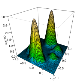
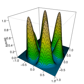
Figure 14: Polar plots of probability densities $|\psi^{(500)}_{(1,3,0)}(r,\phi,\theta)|^{2}$ and $|\psi^{(500)}_{(1,3,\pm 1)}(r,\phi,\theta)|^{2}.$

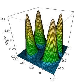
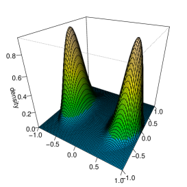
Figure 15: Polar plots of probability densities $|\psi^{(500}_{(1,3,\pm 2)}(r,\phi,\theta)|^{2}$ and $|\psi^{(500)}_{(1,3,\pm 3)}(r,\phi,\theta)|^{2}$

IV.4 Higher excited states, $l\geq 3$ series.

Let us notice that in the matrix re-writing of the eigenvalue problem (5) for $l=0,1,2$ functions, we have encountered the generating matrices (27), (64), (82) respectively, which we list comparatively in a single formula:

$$a_{k,n}^{(0)}=a_{k,n}=2(n+1-k)\,c_{2k},\quad n\geqslant k,$$ (89)

$$a_{k,n}^{(1)}=b_{k,n}=4{\frac{(n+1-k)(n+2-k)}{2n+3-2k}}\,c_{2k},\quad n\geqslant k,$$ (90)

$$a_{k,n}^{(2)}=g_{k,n}=8{\frac{(n+1-k)(n+2-k)(n+3-k)}{(2n+3-2k)(2n+5-2k)}}\,c_{2k},\quad n\geqslant k.$$ (91)

It is clear that we can proceed by induction and take for granted that higher eigenfunctions of the Cauchy well will be determined by linear systems of equations with generating matrices of the form

$$a_{k,n}^{(l)}=2^{l+1}\frac{\prod\limits_{s=1}^{l+1}(n+s-k)}{\prod\limits_{s=1}^{l}(2n+2s+1-2k)}\,\,c_{2k},\quad n\geqslant k,\quad l\geq 0.$$ (93)

We have explicitly (by means of calculations) checked the validity of the formula (93) for the case of $l=3$. The pertinent calculations are skipped here. In particular, for $k=1$ and $l=3$ we have arrived at (approximate) eigenfunctions:

$$\begin{split}\psi_{1,3,0}(\textbf{r})&=C\left(\frac{5x^{3}_{3}-3x_{3}r^{2}}{2}\right)f(r)=C\left(\frac{5\cos^{3}\theta-3\cos\theta}{2}\right)r^{3}f(r)=C^{\prime}r^{3}Y_{3}^{0}(\theta,\phi)f(r),\\ \psi_{1,3,\pm 1}(\textbf{r})&=C(x_{1}\pm x_{2})(5x_{3}^{2}-r^{2})f(r)=C\sin\theta\left(5\cos^{2}\theta-1\right)e^{\pm i\phi}r^{3}f(r)=C^{\prime}r^{3}Y_{3}^{\pm 1}(\theta,\phi)f(r),\\ \psi_{1,3,\pm 2}(\textbf{r})&=C(x_{1}\pm x_{2})^{2}x_{3}f(r)=C\sin^{2}\theta\cos\theta e^{\pm 2i\phi}r^{3}f(r)=C^{\prime}r^{3}Y_{3}^{\pm 2}(\theta,\phi)f(r),\\ \psi_{1,3,\pm 3}(\textbf{r})&=C(x_{1}\pm x_{2})^{3}f(r)=C\sin^{3}\theta e^{\pm 3i\phi}r^{3}f(r)=C^{\prime}r^{3}Y_{3}^{\pm 3}(\theta,\phi)f(r),\end{split}$$ (94)

with a common for all these eigenfunctions $f(r)$ factor of the form

$$f(r)=\sqrt{1-r^{2}}\sum\limits_{n=0}^{\infty}\delta_{2n}r^{2n},\quad\delta_{0}=1.$$ (95)

One readily recognizes both spherical harmonics $Y_{3}^{m}$ and solid harmonics $r^{3}Y_{3}^{m}$ with $m=0,\pm 1,\pm 2,\pm 3$ in the presented formulas. The computed eigenvalue reads $E_{(1,3)}=6.630371$.

Since, in the polynomial approximation of the $2n$-th degree we have computed all expansion coefficients $\delta_{2k}$, we know precisely the functional form of respective (approximate) eigenfunctions. and that of resultant probability densities $\psi_{1,3,m}(r,\phi,\theta)$ with $m=0,\pm 1,\pm 2,\pm 3$. Those are depicted in Figs. (14) - (16).

We stress that the universal form (93) of the generating matrix $a_{k,n}^{(l)}$ opens the door to a direct computation of approximate eigensolutions (eigenvalues and eigenfunctions) for the $l$-the spectral series of arbitrary length, by means of the Wolfram Mathematica routines. Thus, ultimately we are allowed to skip detailed, sometimes tedious and demanding, preliminary calculations, whose outcome would-be the specific (in view of a particular choice of $l$) matrix versions of the spectral problem, like e.g. those encoded in Eqs. (27), (64), (82).

The generic functional form of any trial eigensolution of Eq. (5), corresponding to the eigenvalue $E$ in the $l$-th series, reads as follows:

$$\psi(\textbf{r})=C\,r^{l}\,Y_{l}^{m}(\theta,\phi)\,f(r),$$ (96)

$$f(r)=\sqrt{1-r^{2}}\sum\limits_{n=0}^{\infty}\delta_{2n}r^{2n}.$$ (97)

Actually, in the polynomial approximation of the $2n$-th degree involving $f(r)$ of the form (95) or (97), we end up with a universal (c.f. (93)) matrix eigenvalue problem, valid for any $l=0,1,2,...$, from which one can deduce the corresponding expansion coefficients $\delta_{2k}$, $k\leq n$, with $\delta_{0}=1$ being presumed:

$$\sum\limits_{k=i}^{n}\delta_{2k}a_{k-i,k}^{(l)}=E\sum\limits_{k=0}^{i}\delta_{2k}c_{2(i-k)},\qquad i=0,1,\ldots,n-1,$$

$$\sum\limits_{m=0}^{n}\left(\delta_{2m}\sum\limits_{k=0}^{m}a_{k,m}^{(l)}\right)=0.$$ (98)

The last identity is an outcome of the boundary condition $(-\Delta)^{1/2}\psi(\textbf{r})$ at $r=1$, imposed on the trial function $\psi(\textbf{r})$, Eq. (96), when truncated appropriately (polynomial approximation of the degree $2n$)..

A computer assisted computation, while augmented by an eigenvalue sieve (we order the eigenvalues into the non-decreasing series) allows to associate with each eigenvalue a corresponding eigenstate (or a family of them, in view of the degeneracy of the spectrum). The latter are defined (c.f. (95)) in terms of directly evaluated coefficients $\delta_{2k}$, $k\leq n$, $\delta_{0}=1$ being presumed.

V Outlook

While attempting to solve the spectral problem for the infinite spherical well, we have relied on explicit calculations that show how the nonlocal ultrarelativistic operator acts on properly chosen trial functions in its domain. We have employed an efficient truncation method, which yields approximate eigenvalues and eigenfunctions of the problem, with basically unlimited accuracy (depending on the degree $2n$ of the polynomial truncation).

We have identified universal features of the method of solution, summarized in Eqs. (93), (96)-(98). The structure of the spherical well spectrum resembles that of the standard (Laplacian-induced) quantum mechanical spherical well. Namely, the spectrum splits into non-overlapping eigenvalue and eigenfunction families, each family being labeled by a corresponding orbital label $l=0,1,2,...$. Links of the purely radial family of eigenstates with spectral solutions of the $d=1$ infinite well problem have been established.

In connection with the addressed ultrarelativistic spherical well problem, we refer to Ref. GS for a broader background and rationale for our analysis of nonlocal operators. In the present paper we have contributed to seldom investigated and still unexplored area, where even simplest spectral problems as yet have not received full solutions, specifically those exhibiting nontrivial orbital features.

Like in the standard quantum mechanical reasoning, we regard the infinite well as a an approximation of a deep finite well. Therefore, it is of interest to analyze ind detail the ultrarelativistic finite spherical well (the $d=1$ case has found its solution, ZG ). As well, quite an ambitious research goal could be an analysis a spatially random distribution (”gas”) of finite ultrarelativistic spherical wells, embedded in a spatially extended finite energy background.

References

• (1) P. Garbaczewski and V. Stephanovich, Lévy flights and nonlocal quantum dynamics, J. Math. Phys. 54, (2013) 072103.
• (2) K. Kaleta, M. Kwaśnicki and J. Małecki, One-dimensional quasi-relativistic particle in the box, Rev. Math. Phys. 25 (8), 1350014, (2013).
• (3) P. Garbaczewski and M. Żaba, Nonlocally induced (quasirelativistic) bound states: Harmonic confinement and the finite well, Acta Phys. Pol. 46, 949, (2015).
• (4) Z-F. Li, at al, Relativistic Harmonic Oscillator, J. Math. Phys. 46, 103514, (2005).
• (5) R. L. Hall and W. Lucha, Schrödinger models for solutions of the Bethe-Salpeter equation in Minkowski space, Phys. Rev. D 85, 125006, (2012).
• (6) K. Kowalski and J. Rembieliński,The Salpeter equation and probability current in the relativistic Hamiltonian quantum mechanics, Phys. Rev. A84, 012108, (2011).
• (7) I. W. Herbst, Spectral theory of the operator $(p^{2}+m^{2})^{1/2}-Ze^{2}/r$, Comm.Math. Phys. 53, 285, (1977).
• (8) E. H. Lieb and R. Seiringer, The Stability of Matter in Quantum Mechanics, (Cambridge university Press, 2009).
• (9) I. Białynicki-Birula and Z. Białynicka-Birula, The role of the Riemann-Siberstein vector in classical and quantum theories of electromagnetism, J. Phys. A: Math. Gen. 46, 053001, (2013).
• (10) K. Kowalski and J. Rembieliński, The relativistic massless harmonic oscillator, Phys. Rev. A81, 012118, (2010).
• (11) P. Garbaczewski and V. Stephanovich, Lévy flights in inhomogeneous environments, Physica A 389, 4419, (2010).
• (12) J. Lőrinczi and J. Małecki, Spectral properties of the massless relativistic harmonic oscillator, J. Diff. Equations, 251, 2846, (2012).
• (13) J. Lőrinczi, K. Kaleta and S. Durugo, Spectral and analytic properties of nonlocal Schrödinger operators and related jump processes, Comm. Apppl. Industrial Math. 6(2), e-534, (2015).
• (14) T. Kulczycki, M. Kwaśnicki, J. Małecki, A. Stós, Spectral properties of the Cauchy process on half-line and interval, Proc. London. Math. Soc. 101, 589-622, (2010).
• (15) M. Kwa nicki,Eigenvalues of the fractional Laplace operator in the interval, J. Funct. Anal. 262, 2379, (2012).
• (16) M. Żaba and P. Garbaczewski, Nonlocally-induced (fractional) bound states: Shape analysis in the infinite Cauchy well, J. Math. Phys. 56, 123502, (2015).
• (17) E. V. Kirichenko, P. Garbaczewski, V. Stephanovich, M. Żaba, Infinite Cauchy well spectral solution as the hypersingular Fredholm problem, arXiv:1505.01277 (2015).
• (18) B. Dyda, Fractional calculus for power functions and eigenvalues of the fractional laplacian, Fractional Calculus and Applied Analysis, 15, 4, 536-555, (2012).
• (19) B. Dyda, A. Kuznetsov and M. Kwa nicki, Eigenvalues of the fractional Laplace operator in the unit ball, arXiv:1509.08533 (2015).
• (20) B. Dyda, A. Kuznetsov and M. Kwa nicki, Fractional Laplace operator and Meijer G-function, arXiv:1509.08529 (2015).
• (21) D.J. Griffiths, Introduction to quantum mechanics, (Prentice Hall, NJ, 1995).
• (22) I.S. Gradshteyn and I.M. Ryzhik, Table of Integrals, Series, and Products, Eighth Edition by Daniel Zwillinger and Victor Moll (2014).
• (23) R.R. Liboff, Introductory Quantum Mechanics (4th ed.) (Addison-Wesley, Reading, 2002).
• (24) R. B. Leighton, Principles of Modern Physics, (McGraw-Hill, NY, 1959).