Uncertainty quantification of effective nuclear interactions

Abstract

We give a brief review on the development of phenomenological NN interactions and the corresponding quantification of statistical uncertainties. We look into the uncertainty of effective interactions broadly used in mean field calculations through the Skyrme parameters and effective field theory counter-terms by estimating both statistical and systematic uncertainties stemming from the NN interaction. We also comment on the role played by different fitting strategies on the light of recent developments.

PACS numbers:03.65.Nk,11.10.Gh,13.75.Cs,21.30.Fe,21.45.+v

1 Introduction

The study of nucleon-nucleon (NN) scattering acquired a central role in nuclear physics with the first experimental measurements of neutron-proton (np) and proton-proton (pp) differential cross sections [1, 2]. Since then an ever increasing database of NN scattering measurements at different kinematic conditions has been collected in the literature and several phenomenological potentials have been developed to describe it [3, 4, 5, 6, 7, 8, 9, 10, 11]. However, already in 1935 the seminal work of Yukawa introduced the meson exchange picture where the NN interaction is the result of the exchange of massive particles [12]. This is the basis of the well known one pion exchange potential (OPE) which still nowadays gives the most accurate description of the NN interaction at distances greater than $3.0$ fm. The pioneering work of Gammel and Thaler in 1957 presented an improvement over previous phenomenological approaches by including a spin-orbit coupling term [3] and is considered the first model with a semi-quantitative description of the data [13]. In later years several potentials, including the ones from Hamada-Johnston [4], Yale [5], Paris [6] and Bonn [7] presented gradual improvements by including additional structural terms. For an in depth review of the progress in NN phenomenological interactions before 1993 see Refs. Machleidt:1989tm, Machleidt:1992uz and references therein. Despite the great theoretical efforts to obtain an accurate representation of pp and np elastic scattering data, a statistically successful description of such observables was not possible until 1993 when the Nijmegen group discarded over a thousand $3$ $\sigma$ inconsistent data out of 5246 np and pp scattering observables and incorporated small but relevant electromagnetic effects [16]. After this success a new generation of realistic interactions were introduced including the NijmI, NijmII, Reid93, ArgonneV18 and CD-Bonn potentials [8, 9, 10] as well as the covariant spectator model [17]. A least-squares merit figure yielding $\chi^{2}/{\rm d.o.f.}\lesssim 1$ is a qualifying characteristic for a potential to be considered realistic. As opposed to phenomenological interactions, a fundamental description of NN scattering data should be given by the quantum chromodynamics (QCD) theoretical framework. Using sub-nuclear degrees of freedom in terms of quarks and gluons it is possible, in principle, to describe all levels of hadronic interactions up to nuclear binding. However, despite the tremendous effort done in direct lattice QCD calculations [18, 19, 20] this approach still falls short when confronted with NN scattering data (see however the recent development [21]). Other indirect approaches with QCD ingredients like the inclusion of chiral symmetries in Effective Field Theory (EFT) [22, 23, 24, 25, 26, 27, 28] or large number of colors $N_{c}$ scaling for the NN potential [29, 30, 31, 32, 33] either have a phenomenological component or are unable to accurately reproduce NN scattering observables as high quality interactions up to energies near the pion production threshold (see the discussions in Refs. [34, 35]).

Each experimental measurement of a NN scattering observable is subject to random statistical fluctuations which are quantified by the experimentalist in the form of error bars and in turn create a statistical uncertainty in our knowledge of the NN interaction. In order to determine the size of this statistical uncertainty and provide the NN potential with its corresponding error band an accurate description of the over 8000 pp and np available published data is necessary. Nowadays, phenomenological interactions represent the only approach capable of such a description. Even though the study of the NN interaction started more than six decades ago, the estimation of the corresponding uncertainties has often been overlooked throughout all those years. One of the main reasons behind the lack of estimation of errors arising from experimental uncertainties in pp and np scattering is probably the high level of complexity required to accurately describe the NN interaction, especially when all the details of the short-range or high momentum effects are taken into account directly. Coarse graining embodies the Wilsonian renormalization [36] concept and represents a very reliable tool to simplify the description of pp and np scattering data while still retaining all the relevant information of the interaction up to a certain energy range set by the de Broglie wavelength of the most energetic particle considered. The $V_{\mathrm{low}k}$ potentials in momentum space are a good example of an implementation of coarse graining by removing the high-momentum part of the interaction [37, 38]. Several potentials and partial wave analyses (PWA) which accurately describe a large set of pp and np scattering data can be found in the literature [25, 39, 26, 17, 10, 9, 8, 16]. Despite the great number of experimental data densely probing the NN interaction in certain kinematic regions of energy and scattering angle $(T_{\mathrm{LAB}},\theta)$ other areas of the same plane remain mostly unexplored [40]. This unbalance creates an abundance bias in which different phenomenological potentials show agreement where experimental data are available but great discrepancies can arise when predictions are made for the areas where no data constrains the interaction. Also, each potential has its own particular characteristics, some are given in momentum space, others in coordinate space with different types of non-localities, and some are energy dependent while others are not. These differences in the theoretical representations of the NN interaction combined with the abundance bias of the experimental data gives rise to significant systematic uncertainties which propagate to any nuclear structure calculation and therefore should be quantified to avoid performing nuclear structure calculations with a superfluously high numerical precision.

In this paper we will focus on a particular aspect of error analysis, namely the determination of the low energy structure and its statistical and systematic uncertainties from the point of view of effective interactions.

2 Effective Nuclear Interactions

Power expansions in momentum space of effective interactions were introduced by Moshinsky [41] and Skyrme [42] to provide significant simplifications to the nuclear many body problem in comparison with the ab initio approach, in which it is customary to employ phenomenological interactions fitted to NN scattering data to solve the nuclear many body problem. As a consequence of such simplifications effective interactions, also called Skyrme forces, have been extensively used in mean field calculations [43, 44, 45, 46]. Within this framework the effective force is deduced from the elementary NN interaction and encodes the relevant physical properties in terms of a small set of parameters. However, there is not a unique determination of the Skyrme force and different fitting strategies result in different effective potentials (see e.g. Refs. Friedrich:1986zza and Klupfel:2008af). This diversity of effective interactions within the various available schemes signals a source of statistical and systematic uncertainties that remain to be quantified. Fortunately the parameters determining a Skyrme force can be extracted from phenomenological interactions [49, 50] and uncertainties can be propagated accordingly [51]. At the two body level the Moshinsky-Skyrme potential in momentum representation reads

$$V_{\Lambda}({\bf p}^{\prime},{\bf p}) = \int d^{3}xe^{-i{\bf x}\cdot({\bf p^{\prime}}-{\bf p})}\hat{V}({\bf x})$$ (1)

$$= t_{0}(1+x_{0}P_{\sigma})+\frac{t_{1}}{2}(1+x_{1}P_{\sigma})({\bf p}^{\prime 2}+{\bf p}^{2})$$

$$+t_{2}(1+x_{2}P_{\sigma}){\bf p}^{\prime}\cdot{\bf p}+2iW_{0}{\bf S}\cdot({\bf p}^{\prime}\times{\bf p})$$

$$+\frac{t_{T}}{2}\left[\sigma_{1}\cdot{\bf p}\,\sigma_{2}\cdot{\bf p}+\sigma_{1}\cdot{\bf p^{\prime}}\,\sigma_{2}\cdot{\bf p^{\prime}}-\frac{1}{3}\sigma_{1}\,\cdot\sigma_{2}({\bf p^{\prime}}^{2}+{\bf p}^{2})\right]$$

$$+\frac{t_{U}}{2}\left[\sigma_{1}\cdot{\bf p}\,\sigma_{2}\cdot{\bf p}^{\prime}+\sigma_{1}\cdot{\bf p^{\prime}}\,\sigma_{2}\cdot{\bf p}-\frac{2}{3}\sigma_{1}\,\cdot\sigma_{2}{\bf p^{\prime}}\cdot{\bf p}\right]+{\cal O}(p^{4})$$

where $P_{\sigma}=(1+\sigma_{1}\cdot\sigma_{2})/2$ is the spin exchange operator with $P_{\sigma}=-1$ for spin singlet $S=0$ and $P_{\sigma}=1$ for spin triplet $S=1$ states. The cut-off $\Lambda$ specifies the maximal CM momentum scale, and therefore $\Delta r=\hbar/\Lambda$ determines the de Broglie resolution.

As mentioned above different nuclear data can be used to constrain the Skyrme potential. The usual approach is to fit parameters of Eq. (1) to doubly closed shell nuclei and nuclear matter saturation properties [43, 44, 45, 46]. In Ref. Arriola:2010hj the parameters were determined from just NN threshold properties such as scattering lengths, effective ranges and volumes without explicitly taking into account the finite range of the NN interaction; while in Ref. NavarroPerez:2013iwa the parameters were computed directly from a local interaction in coordinate space that reproduces NN elastic scattering data. In Ref. Perez:2014kpa the latter approach was used to propagate statistical uncertainties into the Skyrme parameters. Here we will follow along the same technique to quantify the systematic uncertainties, which arise from the different representations of the NN interaction. For completeness we reproduce the equations necessary to compute the Skyrme parameters from a local potential in coordinate space:

$$(t_{0},x_{0}t_{0}) = \frac{1}{2}\int\,d^{3}x\,\,\left[V_{{}^{3}S_{1}}(r)\pm V_{{}^{1}S_{0}}(r)\right]\,,$$

$$(t_{1},x_{1}t_{1}) = -\frac{1}{12}\int\,d^{3}x\,r^{2}\,\left[V_{{}^{3}S_{1}}(r)\pm V_{{}^{1}S_{0}}(r)\right]\,,$$

$$(t_{2},x_{2}t_{2}) = \frac{1}{54}\int\,d^{3}x\,r^{2}\,\left[V_{{}^{3}P_{0}}(r)+3V_{{}^{3}P_{1}}(r)+5V_{{}^{3}P_{2}}(r)\pm 9V_{{}^{1}P_{1}}(r)\right]\,,$$

$$W_{0} = \frac{1}{72}\int\,d^{3}x\,r^{2}\,\left[2V_{{}^{3}P_{0}}(r)+3V_{{}^{3}P_{1}}(r)-5V_{{}^{3}P_{2}}(r)\right]\,,$$

$$t_{T} = \frac{1}{5\sqrt{2}}\int\,d^{3}x\,r^{2}\,V_{E_{1}}(r)\,,$$

$$t_{U} = \frac{1}{36}\int\,d^{3}x\,r^{2}\,\left[-2V_{{}^{3}P_{0}}(r)+3V_{{}^{3}P_{1}}(r)-V_{{}^{3}P_{2}}(r)\right]\,,$$ (2)

where the $\pm$ in the first three equations refers to the first and second possibilities on the l.h.s.

Alternatively we consider effective interactions derived from a low momentum interaction where the coefficients can be identified with the phenomenological counter-terms of chiral effective field theory. To obtain such counter-terms we express the momentum space NN potential in the partial wave basis

$$v^{JS}_{l^{\prime},l}(p^{\prime},p)=(4\pi)^{2}\int_{0}^{\infty}\,dr\,r^{2}\,j_{l^{\prime}}(p^{\prime}r)j_{l}(pr)V_{l^{\prime}l}^{JS}(r)\,$$ (3)

and use the Taylor expansion of the spherical Bessel function

$$j_{l}(x)=\frac{x^{l}}{(2l+1)!!}\left[1-\frac{x^{2}}{2(2l+3)}+\dots\right]$$ (4)

to get an expansion for the potential in each partial wave. Keeping terms up to fourth order ${\cal O}(p^{4},p^{\prime 4},p^{3}p^{\prime},pp^{\prime 3},p^{2}p^{\prime 2})$ corresponds to keeping only $S$-, $P$- and $D$-waves along with $S$-$D$ and $P$-$F$ mixing parameters. Using the normalization and spectroscopic notation of Ref. Epelbaum:2004fk one gets

$$v_{00}^{JS}(p^{\prime},p) = \widetilde{C}_{00}^{JS}+C_{00}^{JS}(p^{2}+p^{\prime 2})+D^{1}_{00}{}^{JS}(p^{4}+p^{\prime 4})+D^{2}_{00}{}^{JS}p^{2}p^{\prime 2}+\cdots$$

$$v_{11}^{JS}(p^{\prime},p) = pp^{\prime}C_{11}^{JS}+pp^{\prime}(p^{2}+p^{\prime 2})D_{11}^{JS}+\cdots$$

$$v_{22}^{JS}(p^{\prime},p) = p^{2}p^{\prime}{}^{2}D_{22}^{JS}+\cdots$$

$$v_{20}^{JS}(p^{\prime},p) = p^{\prime}{}^{2}C_{20}^{JS}+p^{\prime}{}^{2}p^{2}D^{1}_{20}{}^{JS}+p^{\prime}{}^{4}D^{2}_{20}{}^{JS}+\dots$$

$$v_{31}^{JS}(p^{\prime},p) = p^{\prime}{}^{3}pD_{31}^{JS}+\cdots$$ (5)

and each counter-term can be expressed as a radial momentum of the NN potential in a specific partial wave. Different methods have been proposed to quantify some of the uncertainties in these quantities[52, 53]. In this work we follow a direct procedure that completely determines the relevant uncertainties.

2.1 Statistical Uncertainties

Most phenomenological interactions are determined by a least squares procedure consisting of the minimization of the figure of merit

$$\chi^{2}=\sum_{i=1}^{N}R_{i}^{2}=\sum_{i=1}^{N}\frac{(O_{i}^{\rm exp}-O_{i}^{\rm theor}(p_{1},p_{2},\ldots,p_{P}))^{2}}{(\Delta O_{i}^{\rm exp})^{2}},$$ (6)

where $O_{i}^{\rm exp}$ are the measured data with an experimental error $\Delta O_{i}^{\rm exp}$, $O_{i}^{\rm theor}$ are the theoretical values determined by the potential parameters $\boldsymbol{p}=(p_{1},p_{2},\ldots,p_{P})$ and $R_{i}$ are known as residuals. The minimization of $\chi^{2}$ corresponds to finding the most likely values for the fitting parameters $\boldsymbol{p}_{0}$ given by

$$\min\chi^{2}(\boldsymbol{p})=\min\sum_{i=1}^{N}\frac{(O_{i}^{\rm exp}-O_{i}^{\rm theor}(\boldsymbol{p}))^{2}}{(\Delta O_{i}^{\rm exp})^{2}}=\chi^{2}(\boldsymbol{p}_{0}).$$ (7)

In practice an agreement between theory and experiment requires $\chi^{2}/(N-P)\sim 1$. But this does not quantify the uncertainty of the parameters after the fit. To obtain statistically justified uncertainties the following crucial property must hold: The discrepancies between theoretical and experimental values are independent and normally distributed. This assumption of course can only be checked after the possibly complex and numerically expensive process of fitting the interaction to reproduce experimental NN scattering data. However, testing for the normality of the residuals is an easy and straightforward procedure, as detailed in Ref. Perez:2014kpa, with a wide range of different tests available in the literature and several of them already implemented in mathematical packages.

Once the assumption of normally distributed residuals has been positively tested it is possible to propagate the experimental uncertainty into the potential parameters in the form of confidence regions via the standard procedure of obtaining the parameters’ covariance matrix. These confidence regions contain the set of values $\boldsymbol{p}^{\prime}$ around $\boldsymbol{p}_{0}$ that give $\chi^{2}(\boldsymbol{p}^{\prime})\leq\chi^{2}(\boldsymbol{p}_{0})+1$ and represent the statistical uncertainty of the phenomenological interaction. The covariance matrix is defined as the inverse of the Hessian matrix

$$({\cal C}^{-1})_{ij}\equiv H_{ij}=\frac{\partial\chi^{2}}{\partial p_{i}\partial p_{j}}$$ (8)

and can be used to calculate the statistical uncertainty of any quantity expressed as a function of the potential parameters

$$(\Delta F)^{2}=\sum_{ij}\frac{\partial F}{\partial p_{i}}\frac{\partial F}{\partial p_{j}}{\cal C}_{ij,}.$$ (9)

Our series of phenomenological interactions, including the DS-OPE, DS-$\chi$TPE, DS-Born, Gauss-OPE, Gauss-$\chi$TPE and Gauss-Born[11, 55, 56, 40, 57], have all been positively and stringently tested for normally distributed residuals. This allows us to confidently propagate the statistical uncertainties into the Skyrme parameters of Eq.(2) and the counter-terms of Eq.(5) using the parameters’ covariance matrix as indicated in Eq.(9). Our results are summarized in tables 2.1 and 2.1. The statistical uncertainties in both the Skyrme parameters and the counter-terms are about the same order of magnitude for the six potentials considered. This was expected since all six interactions are statistically equivalent in the sense that each one describes the self-consistent database with $\chi^{2}/(N-P)\sim 1$ and their residuals follow the standard normal distribution.

Moshinsky-Skyrme parameters for the renormalization scale $\Lambda=400$ MeV. Errors quoted for each potential are statistical; errors in the last column are systematic and correspond to the sample standard deviation of the six previous columns. See main text for details on the calculation of systematic errors. Units are: $t_{0}$ in ${\rm MeV}{\rm fm}^{3}$, $t_{1},t_{2},W_{0},t_{U},t_{T}$ in ${\rm MeV}{\rm fm}^{5}$, and $x_{0},x_{1},x_{2}$ are dimensionless. DS-OPE DS-$\chi$TPE DS-Born Gauss-OPE Gauss-$\chi$TPE Gauss-Born Compilation $t_{0}$ -626.8(64) -529.6(53) -509.0(55) -584.4(157) -406.1(289) -521.8(152) -529.6(751) $x_{0}$ -0.38(2) -0.56(1) -0.54(1) -0.26(2) -0.71(8) -0.55(4) -0.50(16) $t_{1}$ 948.1(30) 913.6(22) 900.1(17) 987.4(29) 945.5(18) 941.3(16) 939.3(304) $x_{1}$ -0.048(3) -0.074(3) -0.068(3) -0.013(3) -0.047(3) -0.058(2) -0.051(22) $t_{2}$ 2462.6(56) 2490.0(39) 2462.1(25) 2441.3(56) 2490.1(24) 2466.8(26) 2468.8(187) $x_{2}$ -0.8686(6) -0.8750(8) -0.8753(6) -0.8630(8) -0.8729(6) -0.8785(3) -0.872(6) $W_{0}$ 107.7(4) 100.8(3) 96.2(3) 105.0(5) 109.3(7) 94.3(2) 102.2(61) $t_{U}$ 1278.6(12) 1260.3(5) 1257.0(4) 1285.6(12) 1254.9(9) 1249.3(3) 1264.3(144) $t_{T}$ -4220.9(87) -4292.8(23) -4289.0(21) -4385.6(99) -4271.8(51) -4319.5(58) -4296.6(545)

Potential integrals in different partial waves. Errors quoted for each potential are statistical; errors in the last column are systematic and correspond to the sample standard deviation of the six previous columns. See main text for details on the calculation of systematic errors. Units are: $\widetilde{C}$’s are in $10^{4}$ ${\rm GeV}^{-2}$, $C$’s are in $10^{4}$ ${\rm GeV}^{-4}$ and $D$’s are in $10^{4}$ ${\rm GeV}^{-6}$. DqS-OPE DS-$\chi$TPE DS-Born Gauss-OPE Gauss-$\chi$TPE Gauss-Born Compilation $\widetilde{C}_{{}^{1}S_{0}}$ -0.141(1) -0.135(2) -0.128(2) -0.121(5) -0.113(9) -0.133(3) -0.13(1) $C_{{}^{1}S_{0}}$ 4.17(2) 4.12(2) 4.04(1) 4.20(2) 4.16(2) 4.18(1) 4.15(6) $D_{{}^{1}S_{0}}^{1}$ -448.8(11) 443.7(5) -441.5(3) -447.0(10) -446.7(2) -446.3(2) -445.7(26) $D_{{}^{1}S_{0}}^{2}$ -134.6(3) -133.1(1) -132.46(4) -134.1(3) -134.02(7) -133.90(7) -133.7(8) $\widetilde{C}_{{}^{3}S_{1}}$ -0.064(2) -0.038(1) -0.039(1) -0.070(2) -0.019(6) -0.038(4) -0.045(19) $C_{{}^{3}S_{1}}$ 3.79(1) 3.55(1) 3.52(1) 4.09(2) 3.785(9) 3.724(9) 3.7(2) $D_{{}^{3}S_{1}}^{1}$ -510.7(3) -504.7(4) -504.1(2) -516.7(6) -509.7(1) -508.2(1) -509.0(46) $D_{{}^{3}S_{1}}^{2}$ -153.2(1) -151.4(1) -151.22(6) -155.0(2) -152.90(3) -152.47(3) -152.7(14) $C_{{}^{1}P_{1}}$ 6.44(2) 6.54(1) 6.464(6) 6.37(2) 6.529(7) 6.488(7) 6.47(6) $D_{{}^{1}P_{1}}$ -594.9(2) -592.1(2) -590.21(6) -594.5(2) -597.83(7) -596.25(7) -594.3(28) $C_{{}^{3}P_{1}}$ 3.738(2) 3.659(3) 3.633(3) 3.762(6) 3.677(3) 3.599(1) 3.68(6) $D_{{}^{3}P_{1}}$ -253.29(5) -249.8(2) -249.62(7) -254.23(9) -251.0(2) -251.06(2) -251.5(19) $C_{{}^{3}P_{0}}$ -4.911(8) -4.882(5) -4.897(3) -4.944(6) -4.802(8) -4.883(2) -4.89(5) $D_{{}^{3}P_{0}}$ 347.0(2) 343.6(2) 344.62(6) 345.8(1) 345.02(3) 346.25(2) 345.4(12) $C_{{}^{3}P_{2}}$ -0.445(2) -0.434(3) -0.426(2) -0.426(2) -0.448(1) -0.427(1) -0.43(1) $D_{{}^{3}P_{2}}$ -10.62(7) -9.7(2) -9.45(6) -11.55(4) -9.939(8) -9.631(7) -10.1(8) $D_{{}^{1}D_{2}}$ -70.92(3) -70.66(6) -70.52(3) -70.58(3) -71.109(7) -71.074(5) -70.8(3) $D_{{}^{3}D_{2}}$ -367.8(2) -364.39(7) -364.54(4) -367.19(8) -367.10(2) -366.99(1) -366.3(15) $D_{{}^{3}D_{1}}$ 205.8(2) 204.25(7) 204.26(4) 204.4(1) 205.17(3) 205.21(3) 204.9(6) $D_{{}^{3}D_{3}}$ 0.55(1) 0.87(6) 0.90(4) -0.32(9) 0.26(3) 0.51(3) 0.46(45) $C_{\epsilon_{1}}$ -8.36(2) -8.500(4) -8.492(4) -8.35(1) -8.404(4) -8.399(5) -8.42(7) $D_{\epsilon_{1}}^{1}$ 1012.6(6) 1005.5(1) 1006.23(6) 1010.5(3) 1011.83(5) 1012.71(6) 1009.9(32) $D_{\epsilon_{1}}^{2}$ 434.0(3) 430.94(4) 431.24(3) 433.1(1) 433.64(2) 434.02(2) 432.8(14) $D_{\epsilon_{2}}$ 84.18(4) 83.29(1) 83.398(7) 84.25(3) 83.660(5) 83.818(8) 83.8(4)

2.2 Systematic Uncertainties

As mentioned earlier the uneven distribution of experimental NN scattering data over the laboratory energy - scattering angle plane creates an abundance bias in which the discrepancies of predictions by phenomenological interactions for observables in unexplored kinematic regions can be significantly larger than the inferred statistical uncertainties. A clear example of this abundance bias is shown in Fig. 1 which plots the polarization transfer parameter $D_{t}$ at $T_{\rm LAB}=325$ MeV as a function of the center of mass scattering angle $\theta_{\rm c.m.}$. For forward scattering angle, where no measurements are available, the six phenomenological potentials show incompatible predictions. This signals the presence of systematic uncertainties arising from the different representations of the NN interaction. In the particular case of the phenomenological interactions listed in tables 2.1 and 2.1 the six potentials can be considered to be statistically equivalent since each one gives an accurate description of the same self-consistent database with normally distributed residuals. Therefore any discrepancy in their predictions can only be attributed to the different representations of the short, intermediate and long range parts. These discrepancies have been observed in phase-shifts, scattering amplitudes and low energy parameters to be considerably larger than the corresponding statistical uncertainties[57].

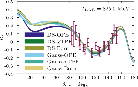
Figure 1: Polarization transfer parameter $D_{t}$ at $T_{\rm LAB}=325$ MeV as a function of center of mass scattering angle $\theta_{\rm c.m.}$. The six bands correspond to the predictions of the six statistically equivalent phenomenological potentials DS-OPE (dark blue), DS-$\chi$TPE (dark green), DS-Born (dark yellow), Gauss-OPE (light blue), Gauss-$\chi$TPE (light green) and Gauss-Born (light yellow). The predictions are compared with experimental data (red error bars) [58, 59].

To estimate the systematic uncertainty on the Skyrme parameters and counter-terms of six statistically equivalent phenomenological interactions presented in the previous section we use the sample standard deviation defined as

$$s=\sqrt{\frac{1}{N-1}\sum_{i=1}^{N}(x_{i}-\bar{x})^{2}},$$ (10)

where $\bar{x}$ is the usual sample mean. The reason for the $1/(N-1)$ factor, instead of the usual $1/N$, is to reduce the bias generated from having an estimate of the mean from a sample of six interactions instead of the actual mean of the population. Of course, this procedure can only give a lower limit of the actual systematic uncertainty since only a subset of all the possible statistically equivalent representations of the NN interaction can be included. Our results are presented in the last column of tables 2.1 and 2.1, with the sample mean as central value. The estimated systematic uncertainties for the Skyrme parameters and counter-terms are always at least an order of magnitude larger than the statistical ones from each one of the six potentials considered. This is in agreement with the results of Ref. Perez:2014waa in phase-shifts, scattering amplitudes and low energy parameters.

3 Discussion on fitting strategies

Our estimates on the statistical and systematic errors of both Skyrme parameters and counter-terms are based on 6 different, statistically significant and equivalent fits to a set of $\sim 6700$ np and pp scattering data below lab energies of $350$ MeV, the canonical and traditional upper energy for NN potentials marked by pion production threshold. They are representative of similar features found previously [57] for phase-shifts, scattering amplitudes and low energy threshold parameters.

3.1 Consistent vs inconsistent fits

Since the earliest fits, the validation of the NN interaction has proceeded normally by the well known least squares $\chi^{2}$-method. This is certainly a convenient and handy way of minimizing discrepancies between the theoretical model characterized by unknown parameters and the available experimental data with their assumed uncertainties. One of the great advantages of the approach is that it has a probabilistic interpretation and relies on a maximum likelihood principle. In the observable space $(O_{1},\dots O_{N})$ the $\chi^{2}$ could be interpreted as a distance enjoying all necessary axioms of a metric measuring the separation between a given theory $O_{i}^{\rm theor}(p_{1},p_{2},\ldots,p_{P})$ and the experimental result $O_{i}^{\rm exp}$ in units of the experimental uncertainties $\Delta O_{i}^{\rm exp}$. Therefore we may understand a sense of proximity within the space of parameters $(p_{1},p_{2},\ldots,p_{P})$. Precisely because of that this is not the only sense of proximity possible, and any other least distance principle might be used to optimize the theory . Of course, alternative approaches provide different senses of optimization but also require more detailed studies and often do not go beyond useful recipes which can hardly be justified a priori nor checked a posteriori.

In contrast, the popularity enjoyed by the traditional least squares approach relies actually in this capability of checking the self-consistency. This is admittedly a potential drawback for the utility of the approach, since one may end up in the uncomfortable situation of having a visually good fit but a mathematically inconsistent one. The fits carried out by ourselves also run these risks. However, we wonder whether it makes sense to take just the advantages of the $\chi^{2}$ without buying the disadvantages. This remark applies beyond the NN data analysis.  As a consequence of this, many of the visually good but inconsistent fits that were found in the process of the present and previous investigations have not been reported. For instance a fit to the full database, without the $3$ $\sigma$ rejection criterion invoked previously [11], provides a $\chi^{2}/{\rm d.o.f.}=1.7$ for about $N\sim 8000$ NN scattering data and corresponds to a discrepancy with the chi square distribution at the $25$ $\sigma$ level. As shown later the re-scaling by a Birge factor [61] cannot be applied as the normality test fails.

Some of the renowned and benchmarking papers on NN fits do not even quote their best $\chi^{2}$ value [4, 7], and it is unclear what they actually mean by improvement beyond a purely visual and subjective inspection of the plots.

For instance, the SAID analysis [62] yields $\chi^{2}/N\sim 1.7$ for the analyzed data bellow laboratory energy of $350$ MeV, which is $25$ $\sigma$ away from any reasonable confidence level. We do not exclude in principle the possibility that a normality test analysis on residuals might allow for re-scaling experimental errors by a Birge factor, something that, to our knowledge, remains to be established. We do not expect, however, this to be the case. The Granada analysis including all $\sim 8000$ NN data is similar in size and provides a similar reduced $\chi^{2}/N\sim 1.7$. Only after self-consistent $3\sigma$ data selection down to $\sim 6700$ data is the normality test passed. The database can be downloaded from Ref. GranadaDB.

Likewise, the widely used Optimized Chiral Nucleon-Nucleon Interaction at Next-to-Next-to-Leading Order [39] fits $N=1945$ scattering NN data for laboratory energies below 125 MeV, yielding a reduced $\chi^{2}/{\rm d.o.f.}=1.15$, already $5$ $\sigma$ excluded as a consistent fit. Unfortunately, as we have recently shown [34], their residuals do not pass the normality test, so that one cannot re-scale by a Birge factor the experimental uncertainties, indicating that the fit is inconsistent. Therefore, either some data are inconsistent among themselves or the proposed theory contains sizable systematic errors.

3.2 Fitting scattering data vs fitting phase-shifts

However, carrying out a large scale PWA implementing all necessary physical effects is rather messy, and one may naturally wonder to what extent all these complications are necessary. Moreover, the main outcome of the PWA are the phase-shifts and mixing parameters. Thus, quite often researchers prefer to fit phase shits from any of the existing data analyses. The key question is: when do the phases extracted from a PWA qualify for tracking the experimental NN uncertainties?. Firstly, one must have for the reduced $\chi^{2}$ a given confidence interval, i.e. $\chi^{2}/{\rm d.o.f.}=1\pm\sqrt{2/{\rm d.o.f.}}$ in order to guarantee a sensible fit with a statistically meaningful confidence level. This is certainly a sufficient condition to carry out a statistically error analysis. Does this mean that if the reduced $\chi^{2}$ does not fall within this range we have a bad fit?. Not necessarily. Fortunately, the reduced $\chi^{2}$ condition is not a necessary one. If the value falls outside this interval, one may still re-scale the errors by a so-called Birge factor, provided one can test positively the hypothesis that the set of residuals are a scaled normal variable. Thus, this requires passing a normality test for the residuals. We have repeatedly stressed this aspect [40, 51] to justify the selection of our database in Ref. Perez:2013jpa and to promote as high quality the 6 interactions proposed by us [57] and used here in our study of Skyrme parameters and counter-terms.

Assuming that all these conditions are fulfilled one would obtain from the PWA a set of phase-shifts with legitimate statistical error bars stemming from experimental uncertainties. Unfortunately, this is a simplifying assumption for it ignores existing correlations among the set of partial waves induced by the fit of scattering observables directly to the available scattering data. Our experience on replacing the full PWA by a reduced set of phase-shifts and mixing parameters is not positive as far as the complete $\chi^{2}/{\rm d.o.f.}$ is concerned. Moreover, this shortcut does not prove to be a faithful determination of statistical errors. This is certainly a regrettable situation which finds its origin, as outlined above, on the lack of control of predicting non-fitted observables, see the discussion around Fig. 1, ultimately triggered by the abundance bias as well as the specific choice of interaction. Under these circumstances we recommended [57] that if a fit to phase-shifts was to be carried out, probably the least biased strategy would be fitting to an average and standard deviation of the 6 proposed potentials, which provides also a larger error bar and for which complete tables are provided. As said, this is based on our own experience on performing fits to single and separate phase-shifts where only statistical error bars were included; the inferred interaction did not reproduce accurately the scattering data from which the phase-shifts being fitted were deduced.

In what follows we comment on recent work where the phase-shift strategy was pursued and also on the possible pitfalls. The local chiral potential suggested in Ref. Gezerlis:2014zia and based on phase-shift fit has been tested in our recent work against the corresponding experimental data within the same energy range [34] providing extremely large reduced $\chi^{2}/N\sim 10-10^{4}$ depending on the maximal energy.

While the calculation in Ref. Epelbaum:2014efa makes, in the authors words, obsolete the widely advertised previous versions, one should say that in line with all their previous developments they have not been confronted with scattering data directly but rather to phase shifts obtained in the SAID analysis [62]. While abundant information regarding good visual fits against selected data is provided, no $\chi^{2}$ to the total number of data used to extract the phase-shifts has been reported. As we pointed out before the, SAID $\chi^{2}/N$ gives $1.7$ for the analyzed data bellow laboratory energy of $350$ MeV, which is $25$ $\sigma$ away from any reasonable confidence level.

Recently a benchmarking analysis of peripheral nucleon-nucleon scattering at fifth order of chiral perturbation theory using input from $\pi N$ scattering was carried out [65]. There a comparison to peripheral phase shifts was shown and good visual agreement can be seen, with the single exception of the ${}^{1}F_{3}$ wave, when compared to the Nijmegen and SAID databases [62] is undertaken. However, as it is well known, peripheral phase-shifts can only be extracted from experiment after a complete PWA, thus they are only indirectly accessible. Besides this, peripheral waves are determined very accurately, as they mostly stem from the OPE potential tail and their error bars are actually tiny. As our recent analysis [57] shows, uncertainties go beyond what a visual fit may discern. Unfortunately, the analysis of Ref. Entem:2014msa does not provide a quantitative measure of the agreement. This is actually a place where a scrupulous error analysis might provide extremely useful information on the validation of the theory.

3.3 Bayesian vs Classical

The Bayesian framework is a particularly appealing approach as it mainly poses the question of the chances for the theory being correct given some data rather than the chances for the data being correct under the assumption that the testing theory is the right one. In the Bayesian interpretation, the fitting parameters become random variables which are determined from the given given data and assuming a prior probability of finding the parameters independently on the experimental data subjected to the analysis. Besides the purely ontological aspects, the Bayesian approach is practical as it educates the theory when the number of parameters and the number of data are similar. A further rewarding aspect of the approach is the asymptotic consistency between both Classical and Bayesian approaches when the number of data actually becomes much larger than the number of parameters.

The practical implementation proceeds via the augmented $\chi^{2}$-approach where an additional term is added to the standard $\chi^{2}$, see Eq. 6, and which will be denoted as $\chi^{2}_{\rm exp}$ here. This new term will be denoted as $\chi^{2}_{\rm th}$ incorporating some a priori known and fuzzy constraints on the fitting parameters and are incorporated as follows (see e.g. Refs. Lepage:2001ym,Morningstar:2001je,Schindler:2008fh for pedagogical introductions)

$$\chi_{\rm th}^{2}=\sum_{i=1}^{P}\left(\frac{p_{i}-p_{i}^{\rm th}}{\Delta p_{i}}\right)^{2},$$ (12)

where one expects the parameters $p_{i}$ to be within $p_{i}^{\rm th}\pm\Delta p_{i}$. The case of absolute ignorance corresponds to $\Delta p_{i}\to\infty$ where the case of absolute certainty corresponds to $\Delta p_{i}\to 0$. Let us denote by $N_{p}$ the number of effective constraints, i.e. the number of parameters where $0<\Delta p_{i}<\infty$. As mentioned, the impact of this new term can only be sizable under certain operating conditions. Namely, $\chi_{\rm exp}^{2}\sim\chi^{2}_{\rm th}$. Otherwise, some ad hoc choice on the relative weight of both contributions has to be made. This is a key question and depends both on the quality of the data as well as the confidence of the constraints. Obviously, for a small number of constraints $N_{p}$ as compared to the number of data or pseudo-data $N_{d}$, a direct addition of $\chi^{2}_{\rm exp}$ and $\chi^{2}_{\rm th}$ would make the constraints irrelevant. Therefore, and following a suggestion [69] one may construct a reduced $\chi^{2}$, $\bar{\chi}^{2}\equiv\chi^{2}/N$, with a $50\%$ weighting on the data/pseudo-data and the theoretical constraints, corresponding to

$$\chi^{2}_{\rm total}\;=\;\frac{N_{d}+N_{p}}{2}\;\left(\frac{\chi^{2}_{\rm exp}}{N_{d}}+\frac{\chi^{2}_{\rm th}}{N_{p}}\right)\,.$$ (13)

The additional terms in the total $\chi^{2}$ impose a penalty for fits which deviate from the $N_{p}$ theoretical expectations on the fitting parameters $p_{i}$ significantly from the a priori theoretical expectation $p_{i}^{\rm th}\pm\Delta p_{i}$. In the case under study corresponding to NN scattering our fitting parameters are the strengths of delta-shells or Gaussian radial functions for which no obvious guess is available. In the present study the counter-terms are taking as derived secondary quantities, but it would certainly be very interesting to test their size in a Bayesian manner based on theoretical expectations deduced either from chiral perturbation theory or large $N_{c}$ arguments as successfully done in a recent meson-meson scattering analysis [69].

Actually, a similar idea was implemented recently [52] to impose the expected $SU(4)$ Wigner symmetry for S-waves, $\tilde{C}_{{}^{1}S_{0}}\sim\tilde{C}_{{}^{3}S_{1}}$, in a Bayesian fashion using the augmented $\chi^{2}$ realization. As we see from Table 2.1 even when we take into account our estimate for the systematic error these two numbers differ.

Of course, one possible interpretation of the Wigner symmetry as a long distance symmetry is Wilsonian in nature as suggested in Ref. Arriola:2010hj and checked within the Similarity Renormalization group approach [70, 71, 72, 73] at relatively small energy scales. In such a case the violation reported in table 2.1 based on a higher energies analysis is not significant as far as the Wigner symmetry analysis is concerned, and may introduce a bias in the Bayesian constraint invoked in Ref. Epelbaum:2014efa.

4 Conclusions

We have extracted the Skyrme parameters of effective interactions from six phenomenological realistic NN interactions. For each potential the statistical uncertainty from the experimental NN scattering data was propagated into the calculated Skyrme parameters. The statistical uncertainties of the parameters are the same order of magnitude for the six potentials. In most cases the extracted Skyrme parameters from different interactions are incompatible within 1 standard deviation. Since the six interactions are statistically equivalent, their discrepancies must originate from the different representations of the NN interaction and are therefore considered to be systematic uncertainties. We estimated the systematic uncertainty of the Skyrme parameters with the sample standard deviation of the six interactions and found it to be at least an order of magnitude larger than the statistical ones. The same procedure was followed to estimate the systematic uncertainties of the counter-terms, which resulted to be also an order of magnitude larger than the statistical ones.

We have also discussed and shown how a detailed statistical scrutiny of the NN scattering data may provide valuable hints on the interplay between theory and experiment and their assumed uncertainties. Ignoring these important pieces of information is not only misleading, but enhances strongly biased views on the underlying dynamical structure of the nuclear force and promoting at the same time interactions which are not properly validated against the available data. These are crucial points for the predictive power of theoretical nuclear physics, since the reliable uncertainty quantification of nuclear forces is an urgent necessity in ab initio nuclear structure and nuclear reactions calculations.

References

- [1] E. Kelly, C. Leith, E. Segrè and C. Wiegand, Phys. Rev. 79 (Jul 1950) 96.
- [2] O. Chamberlain, E. Segrè and C. Wiegand, Phys. Rev. 83 (Sep 1951) 923.
- [3] J. Gammel and R. Thaler, Phys.Rev. 107 (1957) 291.
- [4] T. Hamada and I. Johnston, Nucl.Phys. 34 (1962) 382.
- [5] K. Lassila, M. Hull, H. Ruppel, F. McDonald and G. Breit, Phys.Rev. 126 (1962) 881.
- [6] W. Cottingham, M. Lacombe, B. Loiseau, J. Richard and R. Vinh Mau, Phys.Rev. D8 (1973) 800.
- [7] R. Machleidt, K. Holinde and C. Elster, Phys.Rept. 149 (1987) 1.
- [8] V. Stoks, R. Klomp, C. Terheggen and J. de Swart, Phys.Rev. C49 (1994) 2950, arXiv:nucl-th/9406039 [nucl-th].
- [9] R. B. Wiringa, V. Stoks and R. Schiavilla, Phys.Rev. C51 (1995) 38, arXiv:nucl-th/9408016 [nucl-th].
- [10] R. Machleidt, Phys.Rev. C63 (2001) 024001, arXiv:nucl-th/0006014 [nucl-th].
- [11] R. Navarro Pérez, J. E. Amaro and E. Ruiz Arriola, Phys.Rev. C88 (2013) 064002, arXiv:1310.2536 [nucl-th].
- [12] H. Yukawa, Interaction of elementary particles. Part I, in Proc. Phys. Math. Soc. Jpn., (1935), pp. 48–57.
- [13] R. Machleidt and I. Slaus, J.Phys. G27 (2001) R69, arXiv:nucl-th/0101056 [nucl-th].
- [14] R. Machleidt, Adv.Nucl.Phys. 19 (1989) 189.
- [15] R. Machleidt and G.-Q. Li, Phys.Rept. 242 (1994) 5, arXiv:nucl-th/9301019 [nucl-th].
- [16] V. Stoks, R. Kompl, M. Rentmeester and J. de Swart, Phys.Rev. C48 (1993) 792.
- [17] F. Gross and A. Stadler, Phys.Rev. C78 (2008) 014005, arXiv:0802.1552 [nucl-th].
- [18] S. R. Beane, PoS LATTICE2008 (2008) 008, arXiv:0812.1236 [hep-lat].
- [19] HAL QCD Collaboration (S. Aoki), Prog.Part.Nucl.Phys. 66 (2011) 687, arXiv:1107.1284 [hep-lat].
- [20] HAL QCD Collaboration (S. Aoki et al.), PTEP 2012 (2012) 01A105, arXiv:1206.5088 [hep-lat].
- [21] E. Berkowitz, T. Kurth, A. Nicholson, B. Joo, E. Rinaldi, M. Strother, P. M. Vranas and A. Walker-Loud (2015) arXiv:1508.00886 [hep-lat].
- [22] S. Weinberg, Phys.Lett. B251 (1990) 288.
- [23] C. Ordonez, L. Ray and U. van Kolck, Phys.Rev.Lett. 72 (1994) 1982.
- [24] N. Kaiser, R. Brockmann and W. Weise, Nucl.Phys. A625 (1997) 758, arXiv:nucl-th/9706045 [nucl-th].
- [25] M. Rentmeester, R. Timmermans, J. L. Friar and J. de Swart, Phys.Rev.Lett. 82 (1999) 4992, arXiv:nucl-th/9901054 [nucl-th].
- [26] D. Entem and R. Machleidt, Phys.Rev. C68 (2003) 041001, arXiv:nucl-th/0304018 [nucl-th].
- [27] E. Epelbaum, W. Glockle and U.-G. Meissner, Nucl.Phys. A747 (2005) 362, arXiv:nucl-th/0405048 [nucl-th].
- [28] R. Machleidt and D. Entem, Phys.Rept. 503 (2011) 1, arXiv:1105.2919 [nucl-th].
- [29] H. Muther, C. Engelbrecht and G. Brown, Nucl.Phys. A462 (1987) 701.
- [30] D. B. Kaplan and A. V. Manohar, Phys.Rev. C56 (1997) 76, arXiv:nucl-th/9612021 [nucl-th].
- [31] M. K. Banerjee, T. D. Cohen and B. A. Gelman, Phys.Rev. C65 (2002) 034011, arXiv:hep-ph/0109274 [hep-ph].
- [32] A. Calle Cordon and E. Ruiz Arriola, Phys.Rev. C78 (2008) 054002, arXiv:0807.2918 [nucl-th].
- [33] A. Calle Cordon and E. Ruiz Arriola, Phys.Rev. C80 (2009) 014002, arXiv:0904.0421 [nucl-th].
- [34] R. Navarro Pérez, J. E. Amaro and E. R. Arriola, Phys. Rev. C91 (2015) 054002, arXiv:1411.1212 [nucl-th].
- [35] M. Piarulli, L. Girlanda, R. Schiavilla, R. Navarro Pérez, J. E. Amaro and E. Ruiz Arriola, Phys. Rev. C91 (2015) 024003, arXiv:1412.6446 [nucl-th].
- [36] K. Wilson and J. B. Kogut, Phys.Rept. 12 (1974) 75.
- [37] S. Bogner, T. Kuo and A. Schwenk, Phys.Rept. 386 (2003) 1, arXiv:nucl-th/0305035 [nucl-th].
- [38] S. Bogner, R. Furnstahl and A. Schwenk, Prog.Part.Nucl.Phys. 65 (2010) 94, arXiv:0912.3688 [nucl-th].
- [39] A. Ekström et al., Phys. Rev. Lett. 110 (2013) 192502, arXiv:1303.4674 [nucl-th].
- [40] R. Navarro Pérez, J. E. Amaro and E. Ruiz Arriola, Phys.Rev. C89 (2014) 064006, arXiv:1404.0314 [nucl-th].
- [41] M. Moshinsky, Nuclear Physics 8 (1958) 19 .
- [42] T. Skyrme, Nuclear Physics 9 (1959) 615 .
- [43] D. Vautherin and D. M. Brink, Phys. Rev. C5 (1972) 626.
- [44] J. W. Negele and D. Vautherin, Phys. Rev. C5 (1972) 1472.
- [45] E. Chabanat, J. Meyer, P. Bonche, R. Schaeffer and P. Haensel, Nucl. Phys. A627 (1997) 710.
- [46] M. Bender, P.-H. Heenen and P.-G. Reinhard, Rev. Mod. Phys. 75 (2003) 121.
- [47] J. Friedrich and P. G. Reinhard, Phys. Rev. C33 (1986) 335.
- [48] P. Klupfel, P. G. Reinhard, T. J. Burvenich and J. A. Maruhn, Phys. Rev. C79 (2009) 034310, arXiv:0804.3385 [nucl-th].
- [49] E. Ruiz Arriola (2010) arXiv:1009.4161 [nucl-th].
- [50] R. Navarro Pérez, J. E. Amaro and E. Ruiz Arriola, Few Body Syst. 54 (2013) 1487, arXiv:1209.6269 [nucl-th].
- [51] R. Navarro Pérez, J. E. Amaro and E. Ruiz Arriola, J. Phys. G42 (2015) 034013, arXiv:1406.0625 [nucl-th].
- [52] E. Epelbaum, H. Krebs and U. G. Meißner, Eur. Phys. J. A51 (2015) 53, arXiv:1412.0142 [nucl-th].
- [53] R. J. Furnstahl, N. Klco, D. R. Phillips and S. Wesolowski (2015) arXiv:1506.01343 [nucl-th].
- [54] R. J. Furnstahl, D. R. Phillips and S. Wesolowski, J. Phys. G42 (2015) 034028, arXiv:1407.0657 [nucl-th].
- [55] R. Navarro Pérez, J. E. Amaro and E. Ruiz Arriola, Phys.Rev. C88 (2013) 024002, arXiv:1304.0895 [nucl-th].
- [56] R. Navarro Pérez, J. E. Amaro and E. Ruiz Arriola, Phys.Rev. C89 (2014) 024004, arXiv:1310.6972 [nucl-th].
- [57] R. N. Perez, J. Amaro and E. R. Arriola (2014) arXiv:1410.8097 [nucl-th].
- [58] A. S. Clough et al., Phys. Rev. C21 (1980) 988.
- [59] C. Amsler et al., Phys. Lett. B69 (1977) 419.
- [60] R. Navarro Pérez, E. Ruiz Arriola and J. Ruiz de Elvira, Phys. Rev. D91 (2015) 074014, arXiv:1502.03361 [hep-ph].
- [61] R. T. Birge, Phys. Rev. 40 (Apr 1932) 207.
- [62] W. Briscoe, D. Schott, I. Strakovsky and R. Workman, INS Data Analysis Center http://gwdac.phys.gwu.edu/, Accessed: 2015-08-15.
- [63] R. Navarro Perez, J. Amaro and E. Ruiz Arriola, 2013 Granada Database http://www.ugr.es/~amaro/nndatabase/, (2013), Accessed: 2015-08-15.
- [64] A. Gezerlis, I. Tews, E. Epelbaum, M. Freunek, S. Gandolfi, K. Hebeler, A. Nogga and A. Schwenk, Phys. Rev. C90 (2014) 054323, arXiv:1406.0454 [nucl-th].
- [65] D. R. Entem, N. Kaiser, R. Machleidt and Y. Nosyk, Phys. Rev. C91 (2015) 014002, arXiv:1411.5335 [nucl-th].
- [66] G. P. Lepage, B. Clark, C. T. H. Davies, K. Hornbostel, P. B. Mackenzie, C. Morningstar and H. Trottier, Nucl. Phys. Proc. Suppl. 106 (2002) 12, arXiv:hep-lat/0110175 [hep-lat], [,12(2001)].
- [67] C. Morningstar, Nucl. Phys. Proc. Suppl. 109A (2002) 185, arXiv:hep-lat/0112023 [hep-lat], [,185(2001)].
- [68] M. R. Schindler and D. R. Phillips, Annals Phys. 324 (2009) 682, arXiv:0808.3643 [hep-ph], [Erratum: Annals Phys.324,2051(2009)].
- [69] T. Ledwig, J. Nieves, A. Pich, E. Ruiz Arriola and J. Ruiz de Elvira, Phys. Rev. D90 (2014) 114020, arXiv:1407.3750 [hep-ph].
- [70] V. S. Timoteo, S. Szpigel and E. Ruiz Arriola, Phys. Rev. C86 (2012) 034002, arXiv:1108.1162 [nucl-th].
- [71] E. Ruiz Arriola, V. S. Timoteo and S. Szpigel, PoS CD12 (2013) 106, arXiv:1302.3978 [nucl-th].
- [72] E. Ruiz Arriola, S. Szpigel and V. S. Timoteo, Phys. Lett. B728 (2014) 596, arXiv:1307.1231 [nucl-th].
- [73] E. Ruiz Arriola, S. Szpigel and V. S. Timóteo, Annals Phys. 353 (2014) 129, arXiv:1407.8449 [nucl-th].