Physically feasible three-level transitionless quantum driving with multiple Schrödinger dynamics

Abstract

Three-level quantum systems, which possess some unique characteristics beyond two-level ones, such as electromagnetically induced transparency, coherent trapping, and Raman scatting, play important roles in solid-state quantum information processing. Here, we introduce an approach to implement the physically feasible three-level transitionless quantum driving with multiple Schrödinger dynamics (MSDs). It can be used to control accurately population transfer and entanglement generation for three-level quantum systems in a nonadiabatic way. Moreover, we propose an experimentally realizable hybrid architecture, based on two nitrogen-vacancy-center ensembles coupled to a transmission line resonator, to realize our transitionless scheme which requires fewer physical resources and simple procedures, and it is more robust against environmental noises and control parameter variations than conventional adiabatic passage techniques. All these features inspire the further application of MSDs on robust quantum information processing in experiment.

I Introduction

Accurately controlling a quantum system with high fidelity is a fundamental prerequisite in quantum information processing QIP1 , high precision measurements precision measurement , and coherent control of atomic and molecular systems molecular1 . To this end, rapid adiabatic passage rap , which leads two-level quantum systems to evolve slowly enough along a specific path, can produce near-perfect population transfer between two quantum states of (artificial) atoms or molecules. The adiabatic evolution requires long runtime, which will generate the extra loss of coherence and spontaneous emission of quantum systems. Shortcuts to adiabaticity are alternative fast processes to reproduce the same physical processes in a finite shorter time, which is only limited by the energy-time complementarity qst . There are two potentially equivalent shortcuts to speed up adiabatic process in a nonadiabatic route: Lewis-Riesenfeld invariant-based inverse engineering LR1 ; LR2 ; LR3 ; LR4 ; STAreview and transitionless quantum driving (TQD) TQDA1 ; Rice ; TQDA2 ; TQDA3 ; TQDA5 ; TQDA6 ; dr . Interestingly, TQD has attracted considerable attention in experiment TQDAexperiment ; TQDANV . In 2012, Bason et al. TQDAexperiment demonstrated the quantum system following the instantaneous adiabatic ground state nearly perfectly on Bose-Einstein condensates in optical lattices. In 2013, Zhang et al. TQDANV implemented the assisted adiabatic passages through TQD in a two-level quantum system by controlling a single spin in an nitrogen-vacancy center in diamond.

For three-level quantum systems, the stimulated Raman adiabatic passage (STIRAP) technique STIRAP uses partially overlapping pulses (Stokes and pump pulses) to perfectly realize the population transfer between two quantum states with the same parity, in which single-photon transitions are forbidden by electric dipole radiation. The STIRAP over the rapid adiabatic passage is its robustness against substantial fluctuations of pulse parameters, since the evolution of the quantum system is in the dark state space and only the two quantum states are involved. This technique has gained theoretical and experimental studies in atomic and molecular shore and superconducting quantum systems paraoanu . When TQD is applied to speed up the adiabatic operation in three-level quantum systems, the situation becomes more complicated TQDA3 ; Garaot ; TQDA7 ; TQDA8 ; wei . In 2010, Chen et al. TQDA3 employed the TQD to speed up adiabatic passage techniques in three-level atoms extending to the short-time domain their robustness with respect to parameter variations. In 2014, Martínez-Garaot et al. Garaot studied shortcuts to adiabaticity in three-level systems by means of Lie transforms. Alternatively, in 2012, Chen and Muga chen designed the resonant laser pulses to perform the fast population transfer in three-level systems by invariant-based inverse engineering. In 2014, Kiely and Ruschhaupt ruschhaupt constructed fast and stable control schemes for two- and three-level quantum systems.

Interestingly, multiple Schrödinger dynamics (MSDs) ibanez1 ; ibanez2 were presented to adopt iterative interaction pictures to get physically feasible interactions or dynamics for two-level quantum systems recently. Meanwhile, it enables the designed interaction picture to reproduce the same final population (or state) as those in the original Schrödinger picture by appropriate boundary conditions. In 2012, Ibáñez et al. ibanez1 first employed several Schrödinger pictures and dynamics to design alternative and feasible experimental routes for trap expansions and compressions, and for harmonic transport. In 2013, Ibáñez et al. ibanez2 also examined the limitations and capabilities of superadiabatic iterations to produce a sequence of shortcuts to adiabaticity by iterative interaction pictures. This raises a significative question: whether one can find an effective way for three-level TQD in experimental applications. Three-level quantum systems play important roles in solid-state quantum information processing as they possess some unique characteristics beyond two-level ones, such as electromagnetically induced transparency, coherent trapping, Raman scatting, and so on. Therefore, manipulating such quantum systems in an accurate and robust manner is especially important.

Inspired by the two-level TQD with MSDs ibanez1 ; ibanez2 , here we employ the iteration process to obtain physically feasible TQD in three-level quantum systems. More interestingly, we present a physical implementation for the transitionless scheme with the hybrid quantum system composed of nitrogen-vacancy-center ensembles (NVEs) and the superconducting transmission line resonator (TLR). It has some advantages. First, it can accurately control quantum systems in a shorter time, as adiabatic quantum evolution can be efficiently accelerated by TQD. Second, the MSDs-based Hamiltonian required for three-level TQD is physically feasible, which can be used to implement accurate and robust population transfer and entanglement generation with high fidelity in a single-shot operation. Third, it is more robust against control parameter fluctuations and dissipations than conventional adiabatic passage technique. Fourth, the transitionless scheme presented here is quite universal, and it is broadly applicable in other quantum systems, such as atom cavity, superconducting-qubit TLR, and so on. All these advantages provide the good applications of MSDs on robust quantum information processing in experiment in the future.

This paper is organized as follows: In Sec. II, we show the basic principle of our scheme for obtaining the physically feasible TQD in three-level quantum systems by using MSDs. In Sec.III, we give specific comparisons of population transfer and superposition state generation based on the conventional STIRAP and MSDs, respectively. In Sec. IV, we present a physical implementation of the transitionless scheme on an NVEs-TLR system, and analyze the fidelity in the presence of decoherence. A discussion and a summary are enclosed in Sec. V.

II Physically feasible Hamiltonian with MSDs on three-level quantum systems

II.1 The transitionless Hamiltonian with multiple Schrödinger dynamics

First, we give a brief review of TQD. Considering an arbitrary time-dependent Hamiltonian $H_{0}(t)$ of a quantum system, which has the nondegenerate instantaneous eigenstates $|n_{0}(t)\rangle$ with corresponding eigenvalues $E_{n}(t)$, we get

$$H_{0}(t)|n_{0}(t)\rangle=E_{n}(t)|n_{0}(t)\rangle.$$ (1)

In the adiabatic approximation, the state evolution of the system driven by $H_{0}(t)$ can be written as ($\hbar=1$)

$$|\Psi_{n}(t)\rangle=exp\left\{-i\!\!\int_{0}^{t}\!\!dt^{{}^{\prime}}\!E_{n}(t^{{}^{\prime}})-\!\!\int_{0}^{t}\!\!dt^{{}^{\prime}}\langle n_{0}(t^{{}^{\prime}})|\dot{n_{0}}(t^{{}^{\prime}})\rangle\right\}|n_{0}(t)\rangle.$$ (2)

As a consequence, the evolution operator for this given quantum system is specified. Alternatively, one can seek a transitionless Hamiltonian $H(t)$ that can accurately drive evolving state $|\psi_{n}(t)\rangle$ in a shortest possible time, which guarantees that there are no transitions between the eigenstates of $H_{0}(t)$. That is, it should satisfy

$$H(t)|\psi_{n}(t)\rangle=i|\dot{\psi_{n}}(t)\rangle.$$ (3)

Defining a time-dependent unitary operator

$$\!\!U(t)\!=\!\!\!\sum_{n}\!exp\!\left\{\!-i\!\!\int_{0}^{t}\!\!dt^{{}^{\prime}}\!E_{n}(t^{{}^{\prime}})-\!\!\int_{0}^{t}\!\!dt^{{}^{\prime}}\langle n_{0}(t^{{}^{\prime}})|\dot{n_{0}}(t^{{}^{\prime}})\rangle\!\right\}\!|n_{0}(t)\rangle\langle n_{0}(0)|,$$

which obeys $H(t)U(t)=i\dot{U}(t)$. By analytically solving the equation $H(t)=i\dot{U}(t)U^{{\dagger}}(t)$, we have

$$H(t) = \sum_{n}E_{n}|n_{0}\rangle\langle n_{0}|+i\sum_{n}(|\dot{n_{0}}\rangle\langle n_{0}|-\langle n_{0}|\dot{n_{0}}\rangle|n_{0}\rangle\langle n_{0}|)$$ (5)

$$\equiv H_{0}(t)+H^{cd}_{0}(t),$$

where all kets are time-dependent. From Eq. (5), one can see that the transitionless Hamiltonian $H(t)$ consists of the original Hamiltonian $H_{0}(t)$ for adiabatic evolution and a counterdiabatic driving Hamiltonian $H^{cd}_{0}(t)$ TQDA1 ; Rice ; TQDA2 ; TQDA3 . TQD offers an effective accurate route for the controlled system following perfectly the instantaneous ground state of a given Hamiltonian in theory and experiment. Nevertheless, it is found that the transitionless Hamiltonian is difficult to implement for example in three-level quantum systems TQDA3 since the counterdiabatic driving Hamiltonian has to break down the energy structure of the original Hamiltonian or bring extra detunings.

Superadiabatic iterations as an extension of the usual adiabatic approximation have been introduced in Ref. berry . The process of superadiabatic iteration can be summarized in Table 1, where $H_{j}(t)$ donates the $j-th$ Hamiltonian by a unitary transformation $A_{j-1}(t)$ on the $(j-1)-th$ Hamiltonian $H_{j-1}(t)$, $A_{j}(t)=\sum\limits_{n}|n_{j}(t)\rangle\langle n_{j}(0)|$ ($j=1,2,\cdot\cdot\cdot$), $|n_{j}(t)\rangle$ are the eigenstates of the Hamiltonian $H_{j}(t)$, and $j$ is the number of superadiabatic iteration.

Table 1: Scheme for superadiabatic iteration to realize MSDs as a result of Hamiltonian $H_{0}(t)$.

Iteration	Hamiltonian	Eigenstates	Unitary operator
$0-th$	$H_{0}(t)$	$|n_{0}(t)\rangle$	$A_{0}(t)\!=\!\sum\limits_{n}|n_{0}(t)\rangle\langle n_{0}(0)|$
$1-st$	$H_{1}(t)$	$|n_{1}(t)\rangle$	$A_{1}(t)\!=\!\sum\limits_{n}|n_{1}(t)\rangle\langle n_{1}(0)|$
$\cdot\cdot\cdot\cdot\cdot\cdot$
$j-th$	$H_{j}(t)$	$|n_{j}(t)\rangle$	$A_{j}(t)\!=\!\sum\limits_{n}|n_{j}(t)\rangle\langle n_{j}(0)|$
$\cdot\cdot\cdot\cdot\cdot\cdot$

Here, our goal is to use MSDs to obtain physically feasible transitionless Hamiltonian for three-level quantum systems in TQD. In what follows we will present an explicit explanation about it, reviewing the ideas from Refs. ibanez1 ; ibanez2 . For the initial Hamiltonian $H_{0}(t)$ with eigenstates $|n_{0}(t)\rangle$, the corresponding transitionless Hamiltonian $H^{T}_{0}(t)$ for $0\!-\!th$ iteration reads

$$H^{T}_{0}(t)=H_{0}(t)+H^{cd}_{0}(t)=\sum_{n}E_{n}|n_{0}\rangle\langle n_{0}|+i\dot{A}_{0}(t)A^{{\dagger}}_{0}(t),$$ (6)

where $A_{0}(t)=\sum\limits_{n}|n_{0}(t)\rangle\langle n_{0}(0)|$ is defined as the unitary operator based on the eigenstates $|n_{0}(t)\rangle$ of the initial Hamiltonian $H_{0}(t)$, and $|n_{0}(0)\rangle$ is the bare adiabatic basis. Here, the eigenstates are chosen to fulfill the parallel transport condition, i.e., $\langle n_{0}(t)|\dot{n}_{0}(t)\rangle=0$.

In the first interaction picture (the $1\!-\!th$ iteration), by a unitary transformation $A_{0}(t)$, the interaction picture Hamiltonian $H_{1}(t)$ becomes

$$H_{1}(t)=A^{{\dagger}}_{0}(t)[H_{0}(t)-K_{0}(t)]A_{0}(t).\;\;\;\;\;\;$$ (7)

where $K_{0}(t)=i\dot{A}_{0}(t)A^{{\dagger}}_{0}(t)$. In this case, the transitionless Hamiltonian is described by

$$H^{T}_{1}(t) = A^{{\dagger}}_{0}(t)[H_{0}(t)\!-\!K_{0}(t)\!+\!H^{cd}_{0}(t)]A_{0}(t)$$ (8)

$$= A^{{\dagger}}_{0}(t)H_{0}(t)A_{0}(t).\;\;$$

Here, we employ the relation $K_{0}(t)\!=\!H^{cd}_{0}(t)$. In the Schrödinger picture, the Hamiltonian for TQD is $H_{0}(t)+H^{cd}_{0}(t)$. It is worth noticing that $H^{T}_{0}(t)$ and $H^{T}_{1}(t)$ are related by a unitary transform $A_{0}(t)$, and they represent the same common underlying physics.

In the second interaction picture (the $2\!-\!th$ iteration), for the Hamiltonian $H_{1}(t)$ with eigenstates $|n_{1}(t)\rangle$, the interaction picture Hamiltonian $H_{2}(t)$ can be expressed as

$$H_{2}(t)=A^{{\dagger}}_{1}(t)[H_{1}(t)-K_{1}(t)]A_{1}(t),$$ (9)

where $A_{1}(t)=\sum\limits_{n}|n_{1}(t)\rangle\langle n_{1}(0)|$ and $K_{1}(t)=i\dot{A}_{1}(t)A^{{\dagger}}_{1}(t)$. In the same way, by adding a counterdiabatic driving term, one can obtain another transitionless Hamiltonian $H^{T}_{2}(t)$. Then the Hamiltonian in TQD is $H_{0}(t)+H^{cd}_{1}(t)$, where $H^{cd}_{1}(t)=A_{0}(t)K_{1}(t)A^{{\dagger}}_{0}(t)$.

Similarly, in the high-order interaction picture [the $(j+1)-th$ iteration], one can also get the corresponding Hamiltonian to realize TQD in the Schrödinger picture as

$$H_{0}(t)+H^{cd}_{j}(t)=H_{0}(t)+iB_{j}(t)\dot{A}_{j}(t)A^{{\dagger}}_{j}(t)B^{{\dagger}}_{j}(t),\;\;\;\;\;$$ (10)

where $B_{j}(t)=A_{0}(t)A_{1}(t)\cdot\cdot\cdot A_{j-1}(t)$ and $A_{j}(t)=\sum\limits_{n}|n_{j}(t)\rangle\langle n_{j}(0)|$ ($j=1,2,\cdot\cdot\cdot$) with $|n_{j}(t)\rangle$ being the eigenstates of the Hamiltonian $H_{j}(t)$ for the $j-th$ iteration. Note that a physically feasible Hamiltonian is hard to obtain due to the unpredictable number of superadiabatic iterations needed for execution in the specific quantum systems.

II.2 Physically feasible three-level transitionless quantum driving

In three-level quantum systems, the effective Hamiltonian for achieving adiabatic population transfer in the orthogonal basis of $\{|\phi_{1}\rangle,|\phi_{2}\rangle,|\phi_{3}\rangle\}$ takes the form of

$$H_{0}(t) =\eta\left(\begin{array}[]{ccc}0&0&\cos\theta\\ 0&0&\sin\theta\\ \cos\theta&\sin\theta&0\\ \end{array}\right),$$ (14)

where $\eta=\sqrt{\eta_{1}^{2}+\eta_{2}^{2}}$, $\theta=\arctan(\eta_{1}/\eta_{2})$, and $\eta$, $\eta_{1}$, and $\eta_{2}$ are time-dependent effective coupling strengths. The instantaneous eigenvalues and the corresponding normalized eigenstates are

$$\begin{split}E_{\mp}&=\mp\eta,\;\;\;\;\;E_{0}=0,\\ |E_{-}\rangle&=\frac{1}{\sqrt{2}}(\cos\theta|\phi_{1}\rangle+\sin\theta|\phi_{2}\rangle-|\phi_{3}\rangle),\\ |E_{+}\rangle&=\frac{1}{\sqrt{2}}(\cos\theta|\phi_{1}\rangle+\sin\theta|\phi_{2}\rangle+|\phi_{3}\rangle),\\ |E_{0}\rangle&=\sin\theta|\phi_{1}\rangle-\cos\theta|\phi_{2}\rangle.\end{split}$$ (15)

It is easy to see that $\langle E_{m}|\dot{E}_{m}\rangle=0$ $({m}={+},{-},{0})$. From Eq. (7), one can obtain the interaction picture Hamiltonian in the $1\!-\!th$ iteration for the effective Hamiltonian $H_{0}(t)$ in the basis $\{|E_{-}\rangle,|E_{+}\rangle,|E_{0}\rangle\}$ as follows:

$$H_{1}(t) =\left(\begin{array}[]{ccc}-\eta&0&-\frac{i\dot{\theta}}{\sqrt{2}}\\ 0&\eta&-\frac{i\dot{\theta}}{\sqrt{2}}\\ \frac{i\dot{\theta}}{\sqrt{2}}&\frac{i\dot{\theta}}{\sqrt{2}}&0\\ \end{array}\right),$$ (19)

where $\dot{\theta}=(\dot{\eta}_{1}\eta_{2}-\dot{\eta}_{2}\eta_{1})/\eta^{2}$. The unitary transform matrix related to $H_{0}(t)$ and $H_{1}(t)$ is

$$A_{0} =\left(\begin{array}[]{ccc}\frac{1}{\sqrt{2}}\cos\theta&\frac{1}{\sqrt{2}}\cos\theta&\sin\theta\\ \frac{1}{\sqrt{2}}\sin\theta&\frac{1}{\sqrt{2}}\sin\theta&-\cos\theta\\ -\frac{1}{\sqrt{2}}&\frac{1}{\sqrt{2}}&0\\ \end{array}\right).$$ (23)

The normalized eigenvectors of the Hamiltonian $H_{1}(t)$ are

$$\begin{split}\lambda_{\mp}&=\mp\sqrt{\eta^{2}+\dot{\theta}^{2}},\;\;\;\;\;\lambda_{0}=0,\\ |\lambda_{-}\rangle&=\frac{iW}{R}|E_{-}\rangle+\frac{iQ}{R}|E_{+}\rangle+\frac{\sqrt{2}\dot{\theta}}{R}|E_{0}\rangle,\\ |\lambda_{+}\rangle&=\frac{iQ}{R}|E_{-}\rangle+\frac{iW}{R}|E_{+}\rangle-\frac{\sqrt{2}\dot{\theta}}{R}|E_{0}\rangle,\\ |\lambda_{0}\rangle&=\frac{-i\sqrt{2}\dot{\theta}}{R}|E_{-}\rangle+\frac{i\sqrt{2}\dot{\theta}}{R}|E_{+}\rangle+\frac{2\eta}{R}|E_{0}\rangle,\end{split}$$ (24)

where $W=\eta+\sqrt{\eta^{2}+\dot{\theta}^{2}}$, $Q=-\eta+\sqrt{\eta^{2}+\dot{\theta}^{2}}$, and $R=2\sqrt{\eta^{2}+\dot{\theta}^{2}}$. It generates the unitary operator

$$A_{1} =\left(\begin{array}[]{ccc}\frac{iW}{R}&\frac{iQ}{R}&\frac{-i\sqrt{2}\dot{\theta}}{R}\\ \frac{iQ}{R}&\frac{iW}{R}&\frac{i\sqrt{2}\dot{\theta}}{R}\\ \frac{\sqrt{2}\dot{\theta}}{R}&-\frac{\sqrt{2}\dot{\theta}}{R}&\frac{2\eta}{R}\\ \end{array}\right),$$ (28)

with which one can get the interaction picture Hamiltonian in the $2\!-\!th$ iteration. Substituting Eq. (23) and Eq. (28) into Eq. (10) when $j=1$, one can obtain the Hamiltonian $H_{M}(t)$ in MSDs for realizing shortcuts to adiabaticity as

$$H_{M}(t) =\left(\begin{array}[]{ccc}0&0&\!\!\eta\!\cos\!\theta+V_{1}\\ 0&0&\!\!\eta\sin\!\theta-V_{2}\\ \eta\!\cos\!\theta+V_{1}&\eta\!\sin\theta-V_{2}&0\\ \end{array}\right),$$ (32)

where $V_{1}=4\sin\!\theta(\dot{\eta}\dot{\theta}-\eta\ddot{\theta})/R^{2}$, $V_{2}=4\cos\!\theta(\dot{\eta}\dot{\theta}-\eta\ddot{\theta})/R^{2}$, $\dot{\eta}=(\eta_{1}\dot{\eta_{1}}+\eta_{2}\dot{\eta_{2}})/\eta$, and $\ddot{\theta}=[(\ddot{\eta_{1}}\eta_{2}-\eta_{1}\ddot{\eta_{2}})\eta-2\dot{\eta}(\dot{\eta_{1}}\eta_{2}-\eta_{1}\dot{\eta_{2}})]/\eta^{3}$. It is not difficult to find that the Hamiltonian $H_{M}(t)$ in MSDs has the same form as the Hamiltonian $H_{0}(t)$, without additional couplings and detunings. Thus, a simple and feasible control of TQD for three-level systems is physically implemented with MSDs by flexibly tuning the effective coupling strengths.

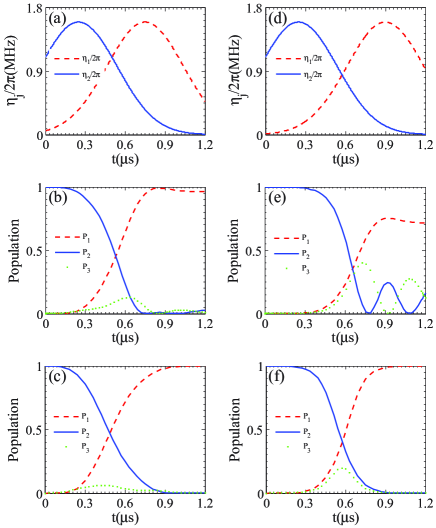
Figure 1: Comparisons of robustness of the population transfer based on the STIRAP and MSDs. (a) The time-dependent effective coupling strengths $\eta_{1}$ and $\eta_{2}$ are in the Gaussian shapes as $\eta_{j}=\eta_{0}e^{-[(t-t_{j})/T]^{2}}$ ($j=1,2$) with $\eta_{0}/{2\pi}=1.6~{}\rm MHz$, $t_{1}=0.75~{}\rm\mu s$, $t_{2}=0.25~{}\rm\mu s$, and $T=0.408~{}\rm\mu s$. Time evolution of the population $P_{k}(t)$ during the population transfer from $|\phi_{2}\rangle$ to $|\phi_{1}\rangle$ based on: (b) STIRAP, and (c) MSDs, respectively. When the time delay of $\eta_{1}$ is changed to be $t_{1}=0.9~{}\rm\mu s$ and other parameters remain invariant, time evolution of the effective coupling strengths and the populations based on STIRAP and MSDs are shown in (d), (e), (f), respectively.

III High-fidelity population transfer and superposition state generation

III.1 Population transfer

From Eq. (15), one can see that when $\theta=0$ at time $t_{i}=0$, the dark state $|E_{0}(t)\rangle$ becomes $|\phi_{2}\rangle$ with a global phase factor $\pi$. If the system evolves adiabatically along the state $|E_{0}(t)\rangle$, the final state is $|\phi_{1}\rangle$ when $\theta=\frac{\pi}{2}$ at later time $t_{f}$. As a result, a simple population transfer is completely realized by STIRAP STIRAP . For this purpose, the time-dependent effective coupling strengths are in the Gaussian shapes as

$$\eta_{j}=\eta_{0}e^{-[(t-t_{j})/T]^{2}},$$ (33)

where $\eta_{0}$, $t_{j}$, and $T$ are the amplitude, time delay, and width of the coupling strength, respectively. In Fig. 1(a), we display variations of the two optimal effective coupling strengths with time $t$ for achieving population transfer, where $\eta_{0}/{2\pi}=1.6~{}\rm MHz$, $t_{1}=0.75~{}\rm\mu s$, $t_{2}=0.25~{}\rm\mu s$, and $T=0.408~{}\rm\mu s$. Figures. 1(b) and 1(c) present time evolution of the populations during the transfer process from $|\phi_{2}\rangle$ to $|\phi_{1}\rangle$ based on STIRAP and MSDs, respectively. The population is defined as $P_{k}(t)=\langle\phi_{k}|\rho(t)|\phi_{k}\rangle$ ($k=1,2,3$) with $\rho(t)$ being the time evolution of density matrix after the population transfer operation on the initial state $|\phi_{2}\rangle$. In this case, both the time evolutions governed by the Hamiltonians $H_{0}(t)$ and $H_{M}(t)$ can achieve near-perfect population transfer from $|\phi_{2}\rangle$ to $|\phi_{1}\rangle$, while the population $P_{3}$ of intermediate state $|\phi_{3}\rangle$ shows a slightly different behavior. When the time delay of $\eta_{1}$ is changed to be $t_{1}=0.9~{}\rm\mu s$, which reduces overlap of the two effective coupling strengths, we plot variations of the effective coupling strengths, time evolution of the populations based on STIRAP and MSDs in Figs. 1(d), 1(e), and 1(f), respectively. One can see that the population transfer by the Hamiltonian $H_{M}(t)$ with MSDs is perfectly realized in a short evolution time, and the final population of the target state $|\phi_{1}\rangle$ can reach $100\%$, while the Hamiltonian $H_{0}(t)$ with STIRAP cannot. Moreover, numerical calculations reveal that the Hamiltonian $H_{M}(t)$ is also valid for high-fidelity population transfer even the time delay of $\eta_{1}$ becomes much bigger than $0.9~{}\rm\mu s$, suggesting that our transitionless scheme with MSDs is very robust and can efficiently realize perfect population transfer.

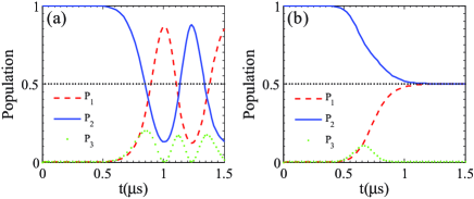
Figure 2: Time evolutions of the populations in the superposition state generation scheme for $|\phi_{1}\rangle$, $|\phi_{2}\rangle$, and $|\phi_{3}\rangle$ based on (a) the STIRAP and (b) MSDs, respectively, with $\eta_{0}/{2\pi}=1.6~{}\rm MHz$, $t_{3}=1.15~{}\rm\mu s$, $t_{4}=0.25~{}\rm\mu s$, and $T=0.408~{}\rm\mu s$.

III.2 Superposition state generation

Assuming the initial state of the system is $|\phi_{2}\rangle$, one can easily get the superposition state $|\psi\rangle=\frac{1}{\sqrt{2}}(|\phi_{1}\rangle-|\phi_{2}\rangle)$ by STIRAP and MSDs. For this purpose, the two time-dependent effective coupling strengths are designed as

$$\begin{split}\eta_{1}&=\eta_{0}e^{-[(t-t_{3})/T]^{2}},\\ \eta_{2}&=\eta_{0}e^{-[(t-t_{4})/T]^{2}}+\eta_{0}e^{-[(t-t_{3})/T]^{2}},\end{split}$$ (34)

which should satisfy the boundary conditions of the STIRAP that at the beginning of the operation $\eta_{1}/\eta_{2}=0$ and at the end $\eta_{1}/\eta_{2}=1$. Given the parameters $\eta_{0}/{2\pi}=1.6~{}\rm MHz$, $t_{4}=0.25~{}\rm\mu s$, and $T=0.408~{}\rm\mu s$, the performances of the populations for $|\phi_{1}\rangle$ and $|\phi_{2}\rangle$ with variation of $t_{3}$ have two conditions as follows: $(\rm{i})$ when the parameter $t_{3}$ gets an optimal time $0.75~{}\rm\mu s$, time evolutions of the populations $P_{1}$ and $P_{2}$ with STIRAP and MSDs reach an approximate value $\frac{1}{2}$, that is, the two approaches effectively generate the superposition state $|\psi\rangle$; $(\rm{ii})$ when $t_{3}$ increases, the population dynamics with STIRAP and MSDs exhibit significantly different behaviors. The equivalent populations with $P_{1}=P_{2}=\frac{1}{2}$ can be implemented with MSDs, implying that time evolution of the quantum state governed by $H_{M}(t)$ is in the superposition state $|\psi\rangle$, while the Hamiltonian $H_{0}(t)$ in STIRAP leads to oscillatory behaviors for $P_{1}$ and $P_{2}$, as shown in Figs. 2(a) and 2(b), respectively. These results convince us that MSDs could pave an efficient way to achieve accurate and robust quantum information processing.

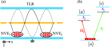
Figure 3: (a) Schematic diagram of the hybrid quantum system, which consists of two NVEs coupled to a high-Q TLR. (b) The $V$-type energy-level configuration for the ground state of NVE driven by the resonator and appropriate external magnetic fields.

IV physical implementation of the transitionless scheme on an NVEs-TLR system

To experimentally realize the population transfer and entanglement generation, we consider the hybrid quantum system, in which two NVEs are coupled to a high-Q TLR, as shown in Fig. 3(a). The NVE can be modeled as a $V$-style three-level qubit with $|g\rangle$ and $|e\rangle$ being two upper-levels, and $|a\rangle$ serving as the lower-level. As illustrated in Fig. 3(b), the transition $|a\rangle\leftrightarrow|e\rangle$ is largely detuned to the resonator frequency with coupling strength $g_{j}$ and detuning $\Delta_{j}$, and the transition $|a\rangle\leftrightarrow|g\rangle$ is off-resonant driven by a time-dependent microwave pulse with Rabi frequency $\Omega_{L,j}(t)$ and the same detuning $\Delta_{j}$, respectively. The interaction Hamiltonian with $\hbar=1$ for the hybrid system is given by

$$H_{I}(t)=\sum_{j=1}^{2}\eta_{j}(t)\,a\sigma_{j}^{{\dagger}}\,+H.c.,$$ (35)

where $\sigma_{j}^{{\dagger}}=|e\rangle_{j}\langle g|$ and $\eta_{j}(t)=g_{\!j}\,\Omega_{L,j}(t)/\Delta_{j}$ is the effective coupling strength. Obviously, it is easy to realize full control of $\eta_{j}(t)$ by changing Rabi frequency $\Omega_{L,j}(t)$ of the microwave pulse when the parameters $g_{j}$ and $\Delta_{j}$ are prescribed. The Hamiltonian $H_{I}(t)$ conserves the total excitation number $N=\sum_{j=1}^{2}\sigma_{j}^{{\dagger}}\sigma_{j}^{-}+n_{c}$ during the dynamical evolution with $n_{c}$ being the photon number in the resonator and $\sigma_{j}^{{\dagger}}=(\sigma_{j}^{-})^{{\dagger}}$. The whole system evolves in the one-excited subspace spanned by $\{|\phi_{1}\rangle=|0ge\rangle,|\phi_{2}\rangle=|0eg\rangle,|\phi_{3}\rangle=|1gg\rangle\}_{c,1,2}$, where the subscripts ${c}$, ${1}$, and ${2}$ donate the resonator mode, the first NVE, and the second NVE, respectively. In the basis of $\{|\phi_{1}\rangle,|\phi_{2}\rangle,|\phi_{3}\rangle\}$, the interaction Hamiltonian $H_{I}(t)$ is equivalent to the Hamiltonian $H_{0}(t)$. Consequently, one can achieve the robust and accurate population transfer and maximally entangled state generation between two NVEs, where the cavity state is employed as an ancillary.

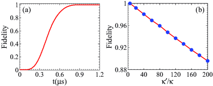
Figure 4: (a) Fidelity of the population transfer scheme with MSDs from $|\phi_{2}\rangle=|0eg\rangle$ to $|\phi_{1}\rangle=|0ge\rangle$ under the influence of dissipations. In the simulation, $\kappa^{-1}=50~{}\rm\mu s$ decay , $\gamma^{-1}=6~{}\rm ms$, $\gamma_{\varphi}^{-1}=600~{}\rm\mu s$ dephasing , and other parameters are the same as those for Fig. 1(c). (b) Fidelity of the population transfer scheme with MSDs for different cavity decay rates $\kappa^{\prime}$ (in units of $\kappa$).

In the presence of dissipations, the dynamics of the NVE-TLR hybrid system is described by the Lindblad master equation:

$$\frac{d\rho}{dt}\!=\!-i\,[H(t),\rho]\!+\!\kappa D[a]\rho\!+\!\gamma D[\sigma^{-}]\rho\!+\!\gamma_{\varphi}D[\sigma^{z}]\rho,$$ (36)

where $\rho$ is the density matrix operator for the hybrid system, $H(t)$ is the Hamiltonian in the form of Eq. (35), $D[L]\rho=(2L\rho L^{+}-L^{+}L\rho-\rho L^{+}L)/2$, $\kappa$ is the decay rate of TLR, and $\gamma$ and $\gamma_{\varphi}$ are the relaxation and dephasing rates of NVE, respectively. For the proposed transfer scheme, the fidelity is defined as $F=\langle\phi_{1}|\rho|\phi_{1}\rangle$ with $|\phi_{1}\rangle$ being the corresponding ideally final state under the population transfer on its initial state $|\phi_{2}\rangle$. By choosing the feasible experimental parameters as: $g/{2\pi}=20~{}\rm MHz$, $\Delta/{2\pi}=200~{}\rm MHz$, $\kappa^{-1}=50~{}\rm\mu s$, $\gamma^{-1}=6~{}\rm ms$, $\gamma_{\varphi}^{-1}=600~{}\rm\mu s$, and $\Omega_{L,j}(t)=\Omega_{0}e^{-[(t-t_{j})/T]^{2}}~{}\rm MHz$ with $t_{1}=0.75~{}\rm\mu s$, $t_{2}=0.25~{}\rm\mu s$, $T=0.408~{}\rm\mu s$, $\Omega_{0}/{2\pi}=16~{}\rm MHz$, which meets the adiabatic condition that $\int_{0}^{\tau}\Omega_{L,j}(t)dt\gg 1$ with $\tau=1.2~{}\rm\mu s$ STIRAP , one can find that the proposed scheme with MSDs can realize perfect population transfer with the fidelity being $100\%$, as shown in Fig. 4(a). To illustrate the robustness of the present scheme, we also simulate the dependence of the fidelity $F$ versus the photon decay rate $\kappa^{\prime}$ in Fig. 4(b). It shows that a high fidelity of $89.60\%$ can still be obtained even for $\kappa^{\prime}/\kappa=200$. The reasons are two-manifold: The cavity state is just used as an ancillary in the present scheme, so it is insensitive to the photon decay in the resonator; the mean photon number $\bar{n}=\langle a^{\dagger}a\rangle$, in consistency with the population $P_{3}$ for intermediate state $|\phi_{3}\rangle$ in Fig. 1, remains a trivial value during the transfer process, which cannot achieve the complete occupation of photon states photon . The above results suggest that time evolution of the populations with MSDs is more robust against control parameter fluctuations and imperfections than STIRAP.

V Discussion and Summary

We consider the feasibility with the current accessible parameters in the NVE-TLR hybrid system. For an NVE placed at the antinodes of the magnetic field of the full-wave mode of the TLR, the coupling strength $g/{2\pi}=16~{}\rm MHz$ between them is reported experimentally NVEs-TLR1 ; photon . The amplitude of microwave pulse is available with the current experiment parameter $\Omega_{0}/{2\pi}=16~{}\rm MHz$ driving . The detuning is $\Delta/{2\pi}=160~{}\rm MHz$ so that $\Delta\gg g$ and $\Delta\gg\Omega_{0}$, which can adiabatically eliminate the state $|a\rangle$. From Eq. (35), the effective coupling strength is $\eta_{j}/{2\pi}=1.6~{}\rm MHz$. When the coupling strength $g$ and detuning $\Delta$ remain invariant, we have full control of the population transfer and entanglement generation by controlling flexibly the time-dependent Rabi frequency $\Omega_{L,j}(t)$ of the microwave pulse with a single-shot operation. The microwave coplanar waveguide resonators with the decay rate of $\kappa^{-1}=50~{}\rm\mu s$ can be reached decay . The dephasing time of $T_{2}>600~{}\mu s$ for an NVE in bulk high-purity diamond has been experimentally observed at room temperature dephasing . An optimized dynamical decoupling microwave pulse has been demonstrated to increase the dephasing time of NVE from $0.7~{}ms$ to $30~{}ms$ DD1 . Moreover, our transitionless scheme with MSDs requires fewer resources, one TLR and two NVEs, which greatly simplifies the experimental complexity.

In summary, we have presented a simple scheme for physically feasible TQD for three-level quantum systems with MSDs, which is used to realize perfect population transfer and entanglement generation in a single-shot operation. Our experimentally realizable transitionless protocol based on the NVE-TLR hybrid system requires fewer physical resources and simple procedures (one-step indeed), works in the dispersive regime, and is robust against decoherence and control parameter fluctuations. These features make our protocol more accurate for the manipulation of the evolution of three-level quantum systems than previous proposals, which may open up further experimental realizations for robust quantum information processing with MSDs.

References

- (1) J. Stolze and D. Suter, Quantum Computing: A Short Course from Theory to Experiment (Wiley-VCH, Berlin, 2008), 2nd ed.
- (2) T. W. Hänsch, Nobel Lecture: Passion for precision. Rev. Mod. Phys. 78, 1297 (2006).
- (3) P. Král, I. Thanopulos, and M. Shapiro, Rev. Mod. Phys. 79, 53 (2007).
- (4) N. V. Vitanov, T. Halfmann, B. W. Shore, and K. Bergmann, Annu. Rev. Phys. Chem. 52, 763 (2001).
- (5) A. C. Santos and M. S. Sarandy, Sci. Rep. 5, 15775 (2015).
- (6) H. R. Lewis and W. B. Riesenfeld, J. Math. Phys. 10, 1458 (1969).
- (7) J. G. Muga, X. Chen, A. Ruschhaupt, E. Torrontegui, and D. Guéry-Odelin, J. Phys. B 42, 241001 (2009).
- (8) X. Chen, E. Torrontegui, and J. G. Muga, Phys. Rev. A 83, 062116 (2011).
- (9) E. Torrontegui, S. Ibáñez, S. Martínez-Garaot, M. Modugno, A. del Campo, D. Guéry-Odelin, A. Ruschhaupt, X. Chen, and J. G. Muga, Adv. At. Mol. Opt. Phys. 62, 117 (2013).
- (10) Y. H. Chen, Y. Xia, Q. Q. Chen, and J. Song, Phys. Rev. A 89, 033856 (2014).
- (11) M. Demirplak and S. A. Rice, J. Phys. Chem. A 107, 9937 (2003).
- (12) M. Demirplak and S. A. Rice, J. Phys. Chem. B 109, 6838 (2005).
- (13) M. Demirplak and S. A. Rice, J. Chem. Phys. 129, 154111 (2008).
- (14) M. V. Berry, J. Phys. A: Math. Theor. 42, 365303 (2009).
- (15) X. Chen, I. Lizuain, A. Ruschhaupt, D. Guéry-Odelin, and J. G. Muga, Phys. Rev. Lett. 105, 123003 (2010).
- (16) A. del Campo, Phys. Rev. Lett. 111, 100502 (2013).
- (17) M. Moliner and P. Schmitteckert, Phys. Rev. Lett. 111, 120602 (2013).
- (18) M. G. Bason, M. Viteau, N. Malossi, P. Huillery, E. Arimondo, D. Ciampini, R. Fazio, V. Giovannetti, R. Mannella, and O. Morsch, Nat. Phys. 8, 147 (2012).
- (19) J. Zhang, J. H. Shim, I. Niemeyer, T. Taniguchi, T. Teraji, H. Abe, S. Onoda, T. Yamamoto, T. Ohshima, J. Isoya, and D. Suter, Phys. Rev. Lett. 110, 240501 (2013).
- (20) K. Bergmann, H. Theuer, and B. Shore, Rev. Mod. Phys. 70, 1003 (1998).
- (21) B. W. Shore, Manipulating Quantum Structures Using Laser Pulses (Cambridge University Press, New York, 2011).
- (22) K. S. Kumar, A. Vepsalainen, S. Danilin, and G. S. Paraoanu, arXiv:1508.02981.
- (23) S. Martínez-Garaot, E. Torrontegui, X. Chen, and J. G. Muga, Phys. Rev. A 89, 053408 (2014).
- (24) M. Lu, Y. Xia, L. T. Shen, J. Song, and N. B. An, Phys. Rev. A 89, 012326 (2014).
- (25) L. Giannelli and E. Arimondo, Phys. Rev. A 89, 033419 (2014).
- (26) X. Shi and L. F. Wei, Laser Phys. Lett. 12, 015204 (2015).
- (27) X. Chen and J. G. Muga, Phys. Rev. A 86, 033405 (2012).
- (28) A. Kiely and A. Ruschhaupt, J. Phys. B 47, 115501 (2014).
- (29) S. Ibáñez, X. Chen, E. Torrontegui, J. G. Muga, and A. Ruschhaupt, Phys. Rev. Lett. 109, 100403 (2012).
- (30) S. Ibáñez, X. Chen, and J. G. Muga, Phys. Rev. A 87, 043402 (2013).
- (31) M. V. Berry, Proc. R. Soc. A 414, 31 (1987).
- (32) A. Megrant, C. Neill, R. Barends, B. Chiaro, Y. Chen, L. Feigl, J. Kelly, E. Lucero, M. Mariantoni, P. J. J. O’Malley, D. Sank, A. Vainsencher, J. Wenner, T. C. White, Y. Yin, J. Zhao, C. J. Palmstrøm, J. M. Martinis, and A. N. Cleland, App. Phys. Lett. 100, 113510 (2012).
- (33) P. L. Stanwix, L. M. Pham, J. R.Maze, D. LeSage, T. K. Yeung, P. Cappellaro, P. R. Hemmer, A. Yacoby, M. D. Lukin, and R. L. Walsworth, Phys. Rev. B 82, 201201 (2010).
- (34) Y. Kubo, C. Grezes, A. Dewes, T. Umeda, J. Isoya, H. Sumiya, N. Morishita, H. Abe, S. Onoda, T. Ohshima, V. Jacques, A. Dréau, J. F. Roch, I. Diniz, A. Auffeves, D. Vion, D. Esteve, and P. Bertet, Phys. Rev. Lett. 107, 220501 (2011).
- (35) Y. Kubo, F. R. Ong, P. Bertet, D. Vion, V. Jacques, D. Zheng, A. Dréau, J. F. Roch, A. Auffeves, F. Jelezko, J. Wrachtrup, M. F. Barthe, P. Bergonzo, and D. Esteve, Phys. Rev. Lett. 105, 140502 (2010).
- (36) G. D. Fuchs, V. V. Dobrovitski, D. M. Toyli, F. J. Heremans, and D. D. Awschalom, Science 326, 1520 (2009).
- (37) D. Farfurnik, A. Jarmola, L. M. Pham, Z. H. Wang, V. V. Dobrovitski, R. L. Walsworth, D. Budker, and N. Bar-Gill, Phys. Rev. B 92, 060301(R) (2015).