Torque-induced rotational dynamics in polymers: Torsional blobs and thinning

Abstract

By using the blob theory and computer simulations, we investigate the properties of a linear polymer performing a stationary rotational motion around a long impenetrable rod. In particular, in the simulations the rotation is induced by a torque applied to the end of the polymer that is tethered to the rod. Three different regimes are found, in close analogy with the case of polymers pulled by a constant force at one end. For low torques the polymer rotates maintaining its equilibrium conformation. At intermediate torques the polymer assumes a trumpet shape, being composed by blobs of increasing size. At even larger torques the polymer is partially wrapped around the rod. We derive several scaling relations between various quantities as angular velocity, elongation and torque. The analytical predictions match the simulation data well. Interestingly, we find a “thinning” regime where the torque has a very weak (logarithmic) dependence on the angular velocity. We discuss the origin of this behavior, which has no counterpart in polymers pulled by an applied force.

]Institute for Theoretical Physics, KU Leuven, Celestijnenlaan 200D, Leuven, Belgium INFN, Sezione di Padova, Via Marzolo 8, Padova, Italy ]Department of Physics, Kyushu University, Fukuoka 819-0395, Japan Laboratoire de Microbiologie et Génétique Moléculaires UMR 5100, CNRS & Université Paul Sabatier, F-31000 Toulouse, France

1 Introduction

Understanding the dynamics of polymers at the nanoscale is a great challenge, which is not only interesting from the conceptual viewpoint, but also because it is useful for applications in nanotechnology. The challenge stems from the fact that even single polymers can display a complex dynamical behavior. A popular example is translocation through a nanopore, a process which has attracted quite some attention in the past years (see Panja et al. and Palyulin et al. ^{1, 2} for a review). In polymer translocation, the molecule is set into motion by an applied field at the pore side which acts as a linear pulling force.

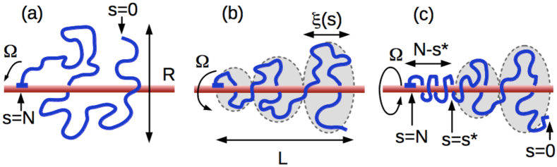
Figure 1: Various dynamical regimes for the steady state motion of a flexible polymer rotating with constant angular velocity $\Omega$ around a rod. (a) The equilibrium regime (small $\Omega$). (b) The trumpet regime (intermediate $\Omega$). (c) The stem-trumpet regime (large $\Omega$). The polymer is attached to the rod at one end $s=N$ while the opposite end ($s=0$) is free, where $s$ labels the monomers along the chain. In the equilibrium regime, the shape is on average spherical with a size $R\simeq aN^{\nu}$. In the trumpet and stem-trumpet regime the polymer conformation is characterized by a series of blob of size $\xi(s)$, which decreases starting from the free end ($s=0$).

While the dynamics of pulled polymers has been thoroughly studied, less attention has been devoted to the properties of polymers performing rotational motion, which can be induced by applying a torque. There are several examples in which the rotational motion of a polymer is of relevance. For instance, in the DNA double helix melting the two strands have to unwind from each other to separate. Another example is the transcription process, where RNA polymerase performs a rotational motion along the DNA axis wrapping the emergent mRNA molecule along the DNA ^{3, 4}. The torque caused by relative rotation of the nascent RNA and DNA during transcription induces dynamic supercoiling in the transcribed DNA (“twin supercoiled domains”) which have a number of biological implications ^{5, 6}. Also the closure of DNA bubbles involves rotational dynamics ^{7, 8} and rotational friction is involved in supercoil formation in DNA ⁹.

The aim of this paper is to investigate the torque-induced dynamics on a flexible polymer using a theoretical model based on torque-balance equations and computer simulations. We find a rich dynamical behavior where the polymer conformation is characterized by three different regimes, illustrated in 1. In general the theoretical predictions are in very good agreement with the simulation results and there are many analogies with the steady state motion of a polymer pulled by a force. In addition, the rotational motion is characterized by a “thinning” regime, which has no analogous counterpart in the dynamics of pulled polymers.

An isolated polymer in equilibrium is characterized by a single length scale, its Flory radius $R\simeq aN^{\nu}$ (where $N$ is the number of monomers and $a$ the monomer-monomer distance). In a polymer subject to confinement or to some external forces, instead, new length scales appear and the aforementioned global scaling generally breaks down. In these cases, the polymer can be described as being composed of blobs ¹⁰ of characteristic size $\xi$. Depending on the system considered, the blobs can have constant size or their size may vary along the chain. According to the blob picture, the equilibrium scaling governed by the Flory exponent $\nu$, still holds at distances below $\xi$, while the effect of the external perturbation becomes apparent at higher distances. A classical illustration of the blob model is a polymer in equilibrium stretched by forces applied at the two end monomers and pointing in opposite direction ¹¹. Here blobs have a characteristic homogeneous size $\xi\simeq k_{B}T/f$, where $f$ is the applied force.

The blob model has been applied to many other equilibrium problems in polymer physics, for instance in modeling dense melts ¹⁰, polyelectrolytes stretched by an applied force ^{12, 13}, polymers and biopolymers confined in nano-channels ^{14, 15, 16} and polymers adsorbed to surfaces ¹⁷. The blob model also provides a powerful tool to study polymer dynamics, a paradigmatic example being a polymer pulled by one end ^{18, 19, 20, 21, 22, 23} (briefly reviewed in the following section). Other out-of-equilibrium cases where the blob model has been applied include the already mentioned polymer translocation ^{24, 23, 22}, the DNA hairpin folding ²⁵, the DNA compression in a nanochannel ²⁶ and the unwinding relaxation of a polymer from a fixed axis ^{27, 28, 29, 4}.

This paper discusses the steady state dynamics of a flexible polymer performing a rotational motion around a fixed and impenetrable rod ^{4, 28}. This motion is induced by a constant torque applied at the one end monomer that is attached to the rod. Hence it is different from the case in which the torque is applied to induce an internal twist dynamics on the polymer ⁹. We consider polymers containing simple single covalent bonds without twisting energy.

After an initial transient regime the polymer performs a steady rotation with a constant angular velocity $\Omega$, which is the rotational counterpart of the steady linear velocity of a polymer pulled by a constant force. To explain the steady state dynamics, we develop a blob model in which torsional blobs have a rotational origin. They have different scaling properties from the tensile blobs arising in stretched or dragged polymers. Our theory shows that, depending on the torque (or angular velocity), the polymer can assume different conformations. For low torques one finds an equilibrium regime (1(a)), followed by a trumpet regime at intermediate torques (1(b)) and a stem-trumpet regime at high $\Omega$ (1(c)). Because of these regimes, the torque grows monotonically but not always linearly with the angular velocity. The theory is supported by Langevin dynamics computer simulations.

2 Theory

It is convenient to recall a few basic properties of polymers pulled at constant force, a case which has been well studied in the past ^{18, 19, 30, 31, 21, 23, 22}. This will allow us to establish some useful scaling relations, which will be compared to those for polymers under torque. The comparison will be made through the introduction of torsional ⁴ blobs. Using the blob model we derive the relation between torque and rotational velocity. Finally the elongation of a self-avoiding polymer along the rod is investigated. Part of the theory of a stationary rotating polymer has already been developed in Ref. ⁴. Here we extend this theory to self-avoiding polymers and compute new quantities as the polymer elongation along the rod, which was not considered previously.

2.1 Tensile blobs

Consider a polymer, consisting of $N$ monomers, pulled by a constant force at one end. To label the monomers along the chain a coordinate $s$ is used: the polymer is pulled at $s=N$, while $s=0$ is the free end. After a transient phase, the polymer arrives in the steady state, moving with a constant velocity ${\mathrm{v}}$. The force difference between two closely lying points $s$ and $s+\mathrm{d}s$ is then fully compensated by the friction. The force balance yields

$$\mathrm{d}f=\gamma_{0}{\mathrm{v}}\mathrm{d}s,$$ (1)

where $\gamma_{0}$ is the friction per monomer. Note that we focus here to the Rouse dynamics case, to which the simple relation (1) applies. With hydrodynamic interactions, the effect of the conformation dependent friction should be taken into account ²². The hydrodynamic case is briefly discussed at the end of this Section.

The differential equation (1) has solution $f(s)=\gamma_{0}{\mathrm{v}}s$, where we used the boundary condition $f(0)=0$. We obtain the following relation between the pulling force $f=f(N)$ and the velocity:

$$f=\gamma_{0}{\mathrm{v}}N.$$ (2)

The force is related to the blob size as

$$\frac{\xi(s)}{a}\simeq\frac{k_{B}T}{f(s)a}\simeq\frac{k_{B}T}{a\gamma_{0}{\mathrm{v}}s}\simeq\frac{a}{\tau_{0}{\mathrm{v}}s},$$ (3)

where we introduced a monomer-scale characteristic time

$$\tau_{0}=\frac{\gamma_{0}a^{2}}{k_{B}T}.$$ (4)

(throughout the paper we use the symbol $\simeq$ to indicate a “quasi-equality” between two quantities, meaning that numerical prefactors of the order unity are neglected). Weak forces do not significantly perturb the shape of the polymer. The threshold force which produces a perturbation can be obtained from the requirement that the size of the initial blob, $\xi(N)$, exceeds the equilibrium radius of the polymer: $\xi(N)\gtrsim aN^{\nu}$. This leads to

$$f\lesssim\frac{k_{B}T}{aN^{\nu}}.$$ (5)

For stronger forces the polymer consists of blobs of varying size and distributed from the free end according to (3), i.e. the blob size grows towards the free end. This so-called trumpet regime ends when the smallest blob has a size comparable to the monomer-monomer distance, i.e. $\xi(N)\simeq a$. The trumpet regime appears for forces in the following range:

$$\frac{k_{B}T}{aN^{\nu}}\lesssim f\lesssim\frac{k_{B}T}{a}\,.$$ (6)

At higher forces,

$$f\gtrsim\frac{k_{B}T}{a},$$ (7)

part of the polymer close to the pulled monomer is stretched, while the end part still has the trumpet shape. For simplicity the boundaries between the three regimes were obtained using static criteria. We note that they can also be obtained from dynamic criteria involving the drift velocity of the polymer. For instance the equilibrium regime can be characterized from the requirement

$${\mathrm{v}}\tau_{R}\lesssim aN^{\nu},$$ (8)

where $\tau_{R}\simeq\tau_{0}N^{1+2\nu}$ is the longest relaxation time. In the relation (8) we require that the distance covered by the polymer in a time equal to $\tau_{R}$ is smaller than its equilibrium radius, i.e. the polymer moves sufficiently slow so that it equilibrates while leaving a region of the size of its radius. It can be easily seen that (8) is identical to (5)). Analogous arguments can be used to derive (6) and (7)).

The three regimes characterized by the inequalities (5)-(7) are the tensile counterparts of those shown in 1 for polymers under torque. For comparison with the rotating polymer it is useful to compute the end-to-end extension of a polymer pulled by a force. In the trumpet regime (6), where the scaling (3) applies to the whole polymer, the end-to-end distance is given by

$$L=\int_{0}^{N}\frac{\xi(s)}{g(s)}\,\mathrm{d}s\,\simeq\frac{a^{2}}{\tau_{0}{\mathrm{v}}}\left(\frac{\tau_{0}{\mathrm{v}}N}{a}\right)^{1/\nu},$$ (9)

where $g(s)\simeq(\xi/a)^{1/\nu}$ is the number of monomers per blob. Note that at the threshold of the equilibrium regime $f\simeq k_{B}T/aN^{\nu}$ the force-velocity relation (2) yields:

$${\mathrm{v}}\simeq\frac{f}{\gamma_{0}N}\simeq\frac{a}{\tau_{0}N^{1+\nu}}.$$ (10)

Substituting this expression in (9) we recover the equilibrium result $L\simeq aN^{\nu}$.

2.2 Torsional Blobs

Consider now the rotational counterpart of a pulled polymer, where a torque $M$ is applied to the monomer attached to the rod ²⁸. For weak torques we expect that, analogous to the case of a pulled polymer, the polymer will perform a rotational motion while maintaining its equilibrium shape. Using the threshold value for the polymer pulled by a constant force (5), an upper bound for the torque in the equilibrium regime is found:

$$M\simeq fR\lesssim k_{B}T.$$ (11)

Here $f$ is the characteristic value of the applied force and $R\simeq aN^{\nu}$ the equilibrium radius. Using $\mathrm{v}\simeq\Omega R$, which relates linear to rotational velocity, together with the force-velocity expression (2), the inequality (11) can be rewritten:

$$\frac{M}{k_{B}T}\simeq\frac{\gamma_{0}N\Omega R^{2}}{k_{B}T}=\tau_{0}\Omega N^{1+2\nu}\lesssim 1.$$ (12)

This establishes the threshold value for the equilibrium regime for given $N$ and $\Omega$ (the characteristic monomer-scale time, $\tau_{0}$, is defined in (4)). Note the similarities of the previous inequality with (8): the inequality in (12) requires the relaxation of the rotating polymer while performing a fraction $1/2\pi$ of a turn. It should be stressed that the condition for the equilibrium regime $M/k_{B}T\lesssim 1$ (11) is correct up to logarithmic terms which, because they are dimensionless, cannot be extracted from scaling considerations. A more accurate handling of these terms is reported in the Section discussing the dependence of the torque on $\Omega$.

We now use a torque balance argument to set up a differential equation for $M(s)$, the torque $M$ as a function of the monomer coordinate $s$. This is the rotational version of (1), which related the force to $s$ in the tensile case. Consider a torsional blob of size $\xi(s)$ which rotates around the rod at fixed angular velocity $\Omega$. The infinitesimal torque difference is $\mathrm{d}M\simeq\xi\mathrm{d}f$, while the friction $\gamma_{0}v\mathrm{d}s\simeq\gamma_{0}\Omega\xi\mathrm{d}s$. The force balance then gives

$$\frac{\mathrm{d}M}{\mathrm{d}s}\simeq\gamma_{0}\Omega\xi^{2}(s).$$ (13)

Unlike in the pulling case, (1), the blob size $\xi(s)$ appears in the previous equation, reflecting the fact that the rotational friction is conformation-dependent even without the hydrodynamic interactions. To close (13), we thus need to know the local relation between the torque and the torsional blob size. To this end we consider the equilibrium properties of a polymer wound around a rod.

The winding angle $\theta$ of a polymer attached to a rod is defined as $2\pi$ times the number of turns the polymer performs around the rod, starting from the fixed end. In equilibrium the average winding angle vanishes by symmetry: $\langle\theta\rangle=0$. This variable is distributed according to the following scaling form ^{32, 33, 34, 35}:

$$P_{\theta}(\theta,N)=f_{\theta}\left(\frac{\theta}{(\ln N)^{\alpha}}\right),$$ (14)

where $f_{\theta}$ is a scaling function. This form is generic, but the case of the two dimensional winding of an ideal polymer around a circle one has $\alpha=1$ ³³. For a two dimensional self-avoiding polymer $\alpha=1/2$ ^{32, 34}. In three dimensions the scaling for the ideal polymer remains $\alpha=1$. The equilibrium three dimensional self-avoiding polymer wound around the rod has been studied numerically ³⁵ and data were fitted with $\alpha\approx 0.75$. In the torque ensemble the probability distribution is obtained by a Laplace transform of (14):

$$P_{M}(M,N) = \int\mathrm{d}\theta\,e^{\beta M\theta}\,P_{\theta}(\theta,N)$$ (15)

$$= f_{M}\left(\frac{M{(\ln N)^{\alpha}}}{k_{B}T}\right).$$

with $f_{M}$ a scaling function. This relation implies that typical values scale as $M\simeq k_{B}T/(\ln N)^{\alpha}$. Applying this result to the torsional blob $\xi(s)\simeq ag(s)^{\nu}$ with $g(s)$ monomers, we get the torsional blob-torque relation

$$M(s) \simeq \frac{k_{B}T}{[\ln{(\xi(s)/a)}]^{\alpha}}$$ (16)

Differentiating the previous relation with respect of $s$ we find:

$$\frac{\mathrm{d}M}{\mathrm{d}s} \simeq -\frac{k_{B}T}{\xi[\ln{(\xi/a)}]^{\alpha+1}}\frac{\mathrm{d}\xi}{\mathrm{d}s}$$ (17)

Combining (13) and (17) we obtain a differential equation for $\xi$. This can be solved explicitely if one neglects the logarithmic term, which has a very weak dependence on $\xi$. The solution is

$$\frac{\xi(s)}{a}\simeq\left(\frac{1}{\tau_{0}\Omega s}\right)^{1/2}.$$ (18)

which agrees with the result of Eq. (46) of Ref. ⁴. Note the central difference with respect to the tensile blobs in (3), where the decay in $s$ is much faster: $\xi\sim 1/s$.

From (18) we get the threshold for the different regimes in the same way as for tensile blobs. Again, the equilibrium regime ends when the equilibrium polymer radius is equal to the size of the initial blob $\xi(N)$, i.e. $\xi(N)\simeq aN^{\nu}$. From this relation, and using (18), we get again (12). The boundary between the trumpet and stem-trumpet regime is obtained when $\xi(N)\simeq a$, which yields

$$\tau_{0}\Omega N\simeq 1\,.$$ (19)

In summary: we expect three distinct regimes, with boundaries given by the analysis above. These regimes are also depicted in 1.

• If $\tau_{0}\Omega\lesssim 1/N^{1+2\nu}$, the polymer rotates while maintaining its equilibrium shape.

• If $1/N^{1+2\nu}\lesssim\tau_{0}\Omega\lesssim 1/N$ the polymer assumes a trumpet shape in its full length. It is composed of torsional blobs of decreasing size $\xi\sim s^{-1/2}$ starting from the free polymer end $s=0$.

• If $\tau_{0}\Omega\gtrsim 1/N$ the polymer assumes a trumpet shape in a limited range $0\leq s\leq s^{*}$, while the monomers close to the tethered point, $s^{*}\leq s\leq N$, are fully wrapped around the rod. This marks the stem-trumpet regime. $s^{*}$, the boundary between stem and trumpet, can be obtained from the relation $\xi(s^{*})/a\simeq 1$, thus:

  $$s^{*}\simeq\frac{1}{\tau_{0}\Omega}\,.$$ (20)

Note that the size of the blob diverges as $s\to 0$. To avoid divergences in the following calculations we compute $\xi_{0}$, the size of the ‘last’ blob, containing $s_{0}$ monomers. The size can be obtained using the blob scaling (18) (recall that $s=0$ is the free end) and the equilibrium properties of the last blob ($\xi_{0}\sim as_{0}^{\nu}$):

$$\frac{\xi_{0}}{a}\simeq\left(\frac{1}{\tau_{0}\Omega}\right)^{1/2}\left(\frac{\xi_{0}}{a}\right)^{-1/2\nu}.$$ (21)

Rewriting yields expressions for $\xi_{0}$ and $s_{0}$:

$$\frac{\xi_{0}}{a}\simeq\left(\frac{1}{\tau_{0}\Omega}\right)^{\nu/(1+2\nu)},$$ (22)

$$s_{0}\simeq\left(\frac{1}{\tau_{0}\Omega}\right)^{1/(1+2\nu)}.$$ (23)

At the threshold between equilibrium and trumpet regime $\tau_{0}\Omega N^{1+2\nu}\simeq 1$ and from (22) one then finds $\xi_{0}\simeq aN^{\nu}$, i.e. the last blob ‘covers’ the whole polymer.

2.3 Torque vs. angular velocity

The analysis of the previous section can be used to compute the total torque applied as a function of the angular velocity. The fact that the rotational friction depends on the conformation leads to a non-trivial dependence of $M$ on $\Omega$.

2.3.1 Equilibrium Regime

To obtain the torque we integrate (13)

$$M\simeq\int_{0}^{N}\mathrm{d}s\,\gamma_{0}\Omega\xi^{2}(s)$$ (24)

When the whole polymer is in equilibrium, random coil statistics holds: $\xi^{2}(s)\simeq a^{2}(N-s)^{2\nu}$. Plugging this into (24) we get

$$\frac{M}{k_{B}T}\simeq\tau_{0}\Omega N^{1+2\nu},$$ (25)

This calculation reproduces (12), which was previously obtained from scaling arguments.

2.3.2 Trumpet Regime

To calculate the torque in the trumpet regime we integrate Eq. (17). We use $\xi$ as integration variable, hence the interval $0\leq s\leq N$ corresponds to $\xi(N)\leq\xi\leq+\infty$, as the last blob size formally diverges in the limit $s\to 0$. Here $\xi(N)$ denotes the size of the first blob. As (17) was obtained from the differentiating (16) we get:

$$M=\int_{0}^{N}\frac{\mathrm{d}M}{\mathrm{d}s}\,\mathrm{d}s\simeq\frac{k_{B}T}{\left[\ln(\xi(N)/a)\right]^{\alpha}}$$ (26)

Using (18) we obtain:

$$\frac{M}{k_{B}T}\simeq\frac{1}{\left[\displaystyle\ln\left(\frac{1}{\sqrt{\tau_{0}\Omega N}}\right)\right]^{\alpha}}$$ (27)

which is a very weakly increasing function of $\Omega$.

We have used Eq. (11) to estimate the boundary between the equilibrium and trumpet regimes. Alternatively we can estimate this boundary by equating the torques of (25) and (26) and assuming that the polymer consists of a single blob $\xi(N)\simeq aN^{\nu}$. We obtain

$$\tau_{0}\Omega N^{1+2\nu}\simeq\frac{1}{\left[\ln N^{\nu}\right]^{\alpha}}$$ (28)

hence the rotating polymer is in equilibrium for torques

$$\frac{M}{k_{B}T}\lesssim\frac{1}{\left[\ln N\right]^{\alpha}}$$ (29)

Compared to (12) the previous relation contains a logarithmic term. In practice this term does not affect strongly the estimate of the boundary of the equilibrium regime. However the estimate (28) is more accurate as it can be seen from a following argument. We can estimate the boundary using

$$M\theta\simeq k_{B}T$$ (30)

where $\theta$ is the stationary winding angle of the rotating polymer. Eq. (30) is the rotational counterpart of the relation $fR\simeq k_{B}T$ (see (5)) which is an estimate of the boundary of the equilibrium regime for a polymer pulled by a force $f$ on one end ($R\simeq aN^{\nu}$ is the Flory radius). In the rotating case the polymer does not display a substantial deformation compared to equilibrium when the average winding is smaller than that from equilibrium fluctuations in absence of torque. The boundary of the equilibrium regime can be estimated by equating the average winding angle induced by the torque to the equilibrium value in absence of torque as follows:

$$\theta\simeq\sqrt{\langle\theta^{2}\rangle_{M=0}}$$ (31)

Now, $\theta$ is obtained from (30), using the torque for the equilibrium regime (25). As equilibrium fluctuations are described by the scaling form (14) we get $\langle\theta^{2}\rangle_{M=0}\sim(\ln N)^{2\alpha}$. Combining these results we get again the relation (28).

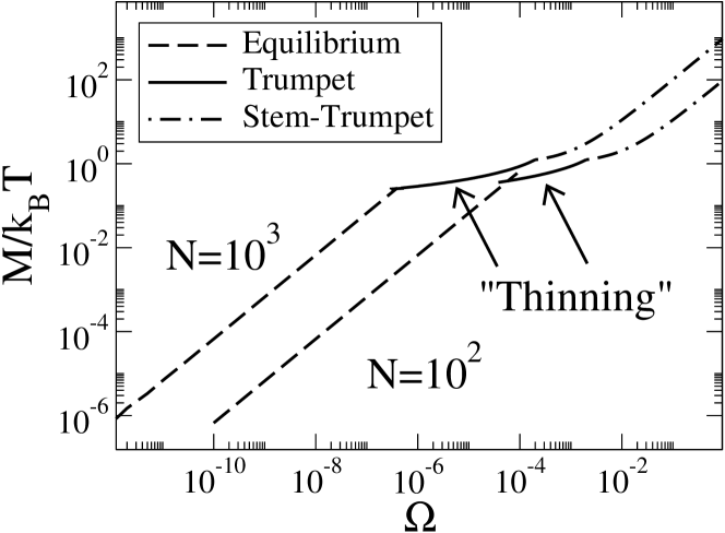
Figure 2: Plots of torque vs. angular velocity predicted by the theory ((25), (27) and (32)), for ideal polymers of two different lengths ($N=10^{2}$ and $N=10^{3}$). The three regimes are highlighted. In the equilibrium regime and in the stem trumpet regime $M$ is linear in $\Omega$ (in the latter asymptotically in $N$). In the intermediate trumpet regime $M$ depends weakly (logarithmically) on $\Omega$. A cutoff value $\Delta=0.2$ was used as estimate the boundary between the trumpet and stem-trumpet regimes.

2.3.3 Stem-Trumpet Regime

In the stem-trumpet regime the polymer is assumed to form a tight helix for $s^{*}\leq s\leq N$, where $s^{*}$ is given by (20) and a trumpet for $s\leq s^{*}$. The contribution of the torque from the stem can be obtained by integrating (18) where the blob size fixed to $\xi\simeq R_{r}$, with $R_{r}$ the radius of the rod. One finds $M_{\rm stem}\simeq\gamma_{0}\Omega R_{r}^{2}(N-s^{*})$. The trumpet part contributes to the torque as (27), with $s^{*}$ replacing $N$. Combining these two contributions results in:

$$\frac{M}{k_{B}T}\simeq\left(\frac{R_{r}}{a}\right)^{2}\left(N-s^{*}\right)\tau_{0}\Omega+\frac{1}{\left[\displaystyle\ln\left(\frac{1}{\sqrt{\tau_{0}\Omega s^{*}}}\right)\right]^{\alpha}}$$ (32)

In this regime the torque is again, to leading order, proportional to $\Omega$. Eq. (19) provides an estimate of the boundary between the trumpet and the stem-trumpet regimes. If this relation is used as a strict equality $\tau_{0}\Omega N=1$ one gets a divergence of (27). Analogously, (32) is divergent when (20) is used as a strict equality. In order to avoid such effects we used in both cases a different cutoff $\tau_{0}\Omega N=\Delta$ and $\tau_{0}\Omega s^{*}=\Delta$, where $\Delta<1$. The torque in the trumpet regime is therefore bounded in the interval:

$$\frac{1}{(\ln N)^{\alpha}}\lesssim\frac{M}{k_{B}T}\lesssim 1$$ (33)

In summary: the torque-angular velocity relation is highly non-trivial, as depicted in 2. At weak and high torques, respectively the equilibrium and stem-trumpet regimes, $M$ is proportional to $\Omega$. This can be directly seen in (25) and (32) (in the latter case this proportionality holds in leading order for large $N$). Both regimes are characterized by two different rotational friction coefficients $M_{\rm C}\simeq\Gamma_{\rm C}\Omega$ and $M_{\rm H}\simeq\Gamma_{\rm H}\Omega$, with different dependencies on the polymer length: $\Gamma_{\rm C}\propto N^{1+2\nu}$ and $\Gamma_{\rm H}\propto N$. In the intermediate trumpet regime there is a strong “thinning” behavior with $M$ increasing very weakly with $\Omega$. Here the polymer decreases its resistance to the rotational motion by getting closer to the rod axis. This contrasts the stretching by a linear force, where the force-velocity relation is always linear for Rouse dynamics, as can be seen by inspection of the force-velocity relation (2). Only for chains with hydrodynamic interactions, a non-linear force-velocity relation is obtained ²².

2.4 Polymer elongation

A self-avoiding polymer is expected to, at sufficiently high torque, elongate as a helix along the rod. The blob theory developed in the previous section can be used to compute the elongation in the three regimes. The elongation, denoted by $L$, is defined as the distance between the two end monomers along the rod direction. In the calculations we can safely use the leading order form for the blob size (18), ignoring higher order logarithmic terms.

2.4.1 Equilibrium regime

In the equilibrium regime the polymer maintains its equilibrium shape, hence

$$L\simeq aN^{\nu}.$$ (34)

2.4.2 Trumpet regime

In the trumpet regime one can simply sum up the contribution of the different blobs:

$$L=\int_{0}^{N}\frac{\xi(s)}{g(s)}\mathrm{d}s,$$ (35)

where $g(s)$ is the number of monomers in the blob. In the calculation there is no need to separate the contribution of the last blob as the singularity in $s\to 0$ is integrable. Using $g(s)\simeq[\xi(s)/a]^{1/\nu}$ and (18), we can evaluate the integral:

$$L\simeq a\int_{0}^{N}\left(\frac{1}{\tau_{0}\Omega s}\right)^{\frac{\nu-1}{2\nu}}\mathrm{d}s\ \simeq\frac{a}{\tau_{0}\Omega}\left(\tau_{0}\Omega N\right)^{\frac{1+\nu}{2\nu}}.$$ (36)

This is the rotational counterpart of (9), which was derived for pulled polymers. The boundary between the equilibrium and the trumpet regime is characterized by the relation $\tau_{0}\Omega\simeq 1/N^{1+2\nu}$. Substituting this boundary condition in (36) gives $L\simeq aN^{\nu}$, as expected in the equilibrium regime. Hence (36) merges with (34) at the phase boundary.

2.4.3 Stem-Trumpet Regime

In the stem-trumpet regime the first $N-s^{*}$ monomers, counting from the end attached to the rod, are fully wrapped around the rod, while the last $s^{*}$ are in a trumpet conformation. Assuming that in the stem the elongation per monomer is $h$, we find

$$L \simeq h(N-s^{*})+a\int_{0}^{s^{*}}\left(\frac{1}{\tau_{0}\Omega s}\right)^{\frac{\nu-1}{2\nu}}\mathrm{d}s\$$ (37)

$$\simeq hN+\frac{a-h}{\tau_{0}\Omega},$$

where we have used (20): $s^{*}\simeq 1/(\tau_{0}\Omega)$. To show the compatibility of (36) and (37), we plug in $\tau_{0}\Omega=1/N$, which marks the phase boundary between trumpet and stem-trumpet regime. It is clear that both expressions then coincide at $L\simeq aN$.

In summary: when the polymer is performing an equilibrium rotation, the elongation along the rod axis is dictated by the random coil value. Upon entering the trumpet regime, blobs start to form and $L$ grows as $\sim\Omega^{(1-\nu)/2\nu}$. Finally, in the stem-trumpet regime the polymer is wrapped around the rod and asymptotically $L\sim N$. Note that in an ideal chain monomers can pass through each other, thus there is no helix formation and the previous calculations are not at issue.

2.5 Hydrodynamics

The results presented above can be extended to the hydrodynamic case. A blob of size $\xi$ moving with velocity $v$ now experiences a friction propotional to its size, $\gamma_{0}v\xi/a$, while without hydrodynamics the friction scales with the number of monomers in a blob. The contribution of a small segment $\mathrm{d}s$ of the polymer to the friction force is then

$$\mathrm{d}f=\gamma_{0}v\left(\xi/a\right)\frac{\mathrm{d}s}{\left(\xi/a\right)^{1/\nu}}.$$ (38)

Hence the torque balance ($\mathrm{d}M=\xi\mathrm{d}f$) reads

$$\frac{\mathrm{d}M}{\mathrm{d}s}\simeq\gamma_{0}a^{2}\Omega\left(\frac{\xi}{a}\right)^{3-1/\nu},$$ (39)

which is the counterpart of (13).

(17) was derived from local equilibrium input, hence it remains valid in the hydrodynamic case. Combining (17) and (39) results in a differential equation for $\xi(s)$. The solution, neglecting again logarithmic terms, is

$$\xi(s)\simeq\left(\frac{1}{\tau_{0}\Omega s}\right)^{\frac{\nu}{3\nu-1}}.$$ (40)

Using the Flory exponent $\nu=3/5$ we get $\xi\sim s^{-3/4}$. This is a more rapid decay of the blob size than in the Rouse case $\sim s^{-1/2}$, see Eq.(18).

Using (40) we can calculate the scaling behavior of various quantities in the hydrodynamic case. Note that (26) implies that $M$ still depends logarithmically on $\Omega$ in the trumpet regime. Another interesting quantity to compute is the elongation in the trumpet regime:

$$L=\int_{0}^{N}\frac{\xi(s)}{g(s)}\mathrm{d}s\simeq\frac{a}{\tau_{0}\Omega}\left(\tau_{0}\Omega N\right)^{\frac{2\nu}{3\nu-1}}.$$ (41)

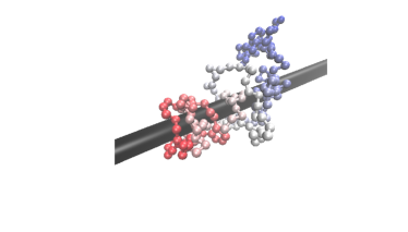
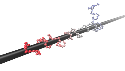
Figure 3: Snapshots of simulations of steady rotating polymers around an infinitely long rod. The figure shows an ideal polymer (left) where excluded volume interactions are only between each monomer and the rod and a real polymers (right) where excluded volume interactions act between all monomers as well. The first monomer in the red end is attached to the rod and is subjected to an external torque. The torque has the value $M=3.55$ and the length is $N=200$ in both cases, which corresponds to the trumpet regime.

3 Numerical Simulations

Numerical simulations were performed using the LAMMPS package ³⁶. Due to the large computational cost of simulating systems with hydrodynamics interactions, we restrict our analysis to simulations of Rouse polymers. The polymer was modeled using a bead spring model with a finitely extensible nonlinear elastic (FENE) interaction ³⁷ between successive beads, so that a maximal distance between bonds is imposed. The rod was modeled by defining a cylindrical region with radius $R_{r}$ around the z-axis and adding soft repulsive interaction of Weeks-Chandler-Andersen (WCA) type ³⁸. Because the maximal distance between beads is chosen smaller than the diameter of the rod, it is impossible for bonds to cross through the rod.

In order to impose a constant torque we introduced a ‘ghost’ particle at the origin of the axes, i.e. within the rod. A second particle was kept at a constant distance from it using the SHAKE algorithm ³⁹. The distance was set equal to $R_{r}$, the radius of the rod. A constant force $f_{b}$ was applied to the second particle, which corresponds to the first bead of the polymer. This force was oriented perpendicular to the plane defined by the rod and the axis connecting this first bead and the ghost particle. The applied torque equals then $M=f_{b}R_{r}$. Furthermore LJ units of LAMMPS were used, such that $k_{B}=m=1$. In these units the two parameters controlling the repulsive Lennard-Jones part of the FENE potential (usually called $\epsilon$ and $\sigma$) are also set to one. Then we chose to set $\gamma_{0}=a=R_{r}=1$. The maximal bond length, controlled by the FENE potential, was set to 1.5.

The system was integrated using the fix nve and fix langevin commands in LAMMPS, which corresponds to performing a Langevin dynamics simulation. Time integration is realized using a velocity Verlet updating scheme. The coupling to the heat bath is implemented through the thermostat described in Schneider and Stoll⁴⁰ and Dunweg and Paul⁴¹. Simulations were performed for different torques and for lengths up to $N=400$. 3 shows two snapshots of the simulations, representing the two models used in the simulations: ideal polymers (left) and self-avoiding polymers (right). In the latter case an additional WCA potential was added.

In the simulations the torque is fixed and applied to the anchored monomer. Thus there are no numerical errors on $M$. The angular velocity was instead determined from the simulation runs. For every value of the applied torque the simulation was run for a significantly long time, such that the stationary state was reached. The angular velocity was determined by counting the number of turns a monomer made in a given time interval, multiplying this number by $2\pi$ and dividing by the length of the time interval. Monomers close to the attached end have larger fluctuations, so $\Omega$ was estimated by averaging over the end monomers.

In this section we focus on three observables. The first is the blob size along the rod. Due to its interesting properties, a separate section for the size of the last blob is added. Then the focus shifts to the torque versus angular velocity relation. Finally the elongation of a SAW along the rod is presented.

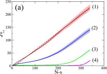
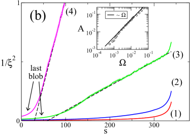
Figure 4: Plots of (a) $\xi^{2}$ vs. $N-s$ and (b) $1/\xi^{2}$ vs. $s$ for an ideal polymer of length $N=340$ and for three different angular velocities: (1) $\Omega=5.17\cdot 10^{-5}$, (2) $\Omega=1.55\cdot 10^{-4}$, (3) $\Omega=5.61\cdot 10^{-4}$ and (4) $\Omega=8.19\cdot 10^{-4}$. The standard error is depicted as a shade around the plots.

3.1 Blob size vs. $s$

First of all we are interested in the blob size. A good estimator for this blob size is the average distance of each monomer from the rod. As the rod is oriented along the z-axis we have

$$\xi(s)=\sqrt{x^{2}(s)+y^{2}(s)},$$ (42)

where $x(s)$ and $y(s)$ represent the x- and y-coordinate of the $s$-th monomer.

In 4(a), $\xi^{2}(s)$ vs. $N\!-\!s$ is presented for four different values of the applied torque, for ideal polymers. These four cases are labeled from 1 to 4, ordered according to increasing applied torque. We estimated the stationary angular velocity $\Omega$, for the different cases, as presented in the caption, from the ratio of the number of turns of each monomer over the simulation time.

For case 1, the weakest applied torque, the polymer has an equilibrium shape characterized by random coil scaling (recall that $s\!=\!0$ is the free end):

$$\xi^{2}(s)\simeq a^{2}(N-s)^{2\nu},$$ (43)

with $\nu=1/2$ for ideal polymers. In this case we estimate $\tau_{0}\Omega N^{2}\!\approx\!6$, using $\tau_{0}\!=\!1$ and setting $\Omega$ as given in the caption of 4. Since $\tau_{0}\Omega N^{1+2\nu}\!>\!1$, this should correspond to the trumpet regime - according to the analysis in the theory section. However, the theory is based on scaling arguments and the relations are valid up to some numerical prefactors. This first case (1) suggests that the trumpet regime sets in at $\Omega$’s a bit higher than predicted by (12).

When higher torques are applied (cases 2-4) the stationary shape gets distorted from the equilibrium. The polymer gets wrapped around the rod, but close to the free end $s\!=\!0$ the shape is well fitted by (43), indicating that the free end is equilibrated. For case 4 we get $\tau_{0}\Omega N\!\approx\!0.3$, indicating that the system is close to the onset of the stem-trumpet regime, see (19).

In order to check the validity of the blob theory we have replotted the data of 4(a) in 4(b), but in the form $1/\xi^{2}$ vs. $s$. The data of cases 3 and 4 are well fitted by a linear form

$$\frac{1}{\xi^{2}}=As+B$$ (44)

which supports the scaling form of (18). In fitting the data we used a non vanishing intercept $B$, due to the correction from the last blob. In case 2 the last blob seems to be extended to the whole polymer and the scaling $1/\xi^{2}\sim s$ cannot be clearly observed. We have fitted the data of $1/\xi^{2}$ vs. $s$ in the range of values where this relation is linear using a two-parameter fit on (44). The slope coefficient $A$ as a function of $\Omega$ is shown in the inset of 4(b). This quantity increases linearly with $\Omega$ in agreement with the prediction of (18). A similar analysis was performed for self-avoiding polymers. The results are in agreement with the blob theory and are shown in 5(a,b). Close to the free end the polymer exhibits equilibrium scaling $\xi^{2}\sim(N-s)^{2\nu}$ (5(a)). The plot $1/\xi^{2}$ vs. $s$ (5(b)) shows the characteristic scaling behavior $\sim 1/\sqrt{s}$ of torsional blobs (18).

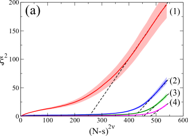
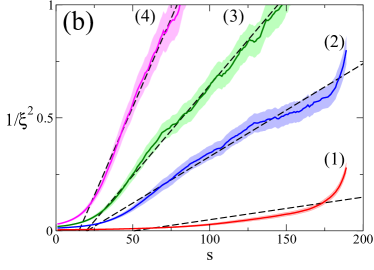
Figure 5: Plots of (a) $\xi^{2}$ vs. $(N-s)^{2\nu}$ ($\nu=0.588$) and (b) $1/\xi^{2}$ vs. $s$ for a self-avoiding polymer of length $N=190$ and for three different angular velocities: (1) $\Omega=1.95\cdot 10^{-4}$, (2) $\Omega=1.16\cdot 10^{-3}$, (3) $\Omega=2.34\cdot 10^{-3}$ and (4) $\Omega=4.01\cdot 10^{-3}$. The standard error is depicted as a shade around the plots.

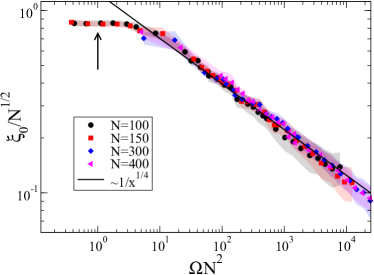
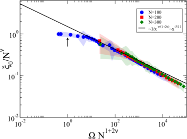
Figure 6: Plot of $\xi_{0}/N^{1/2}$ vs. $\Omega N^{1+2\nu}$ for (a) an ideal polymer ($\nu=1/2$) and (b) a self-avoiding polymer ($\nu=0.588$). The data for different lengths collapse into a single master curve as predicted from (45). The scaling function governs the crossover from equilibrium to trumpet regime, expected to take place for $\tau_{0}\Omega N^{1+2\nu}\simeq 1$, see (12). This value is indicated by a vertical arrow. Recall that in the simulation units $\tau_{0}\simeq 1$. The standard error is depicted as a shade around the plots.

3.2 The last blob

We focus now on the size of the last blob $\xi_{0}$. In the trumpet regime, according to (22), $\xi_{0}\!\sim\!\Omega^{-\nu/(1+2\nu)}$, while in the equilibrium case $\xi_{0}\!\simeq\!aN^{\nu}$. We can connect the two regimes using the following ansatz:

$$\xi_{0}=aN^{\nu}\,\phi\left(\tau_{0}\Omega N^{1+2\nu}\right),$$ (45)

where $\phi(x)$ is a scaling function and the scaling variable $x\!\equiv\!\tau_{0}\Omega N^{1+2\nu}$, which is the natural combination of $\Omega$ and $N$ (see (12)). The equilibrium regime is recovered in the limit of small $x$ if $\phi(x)\to\phi_{0}\simeq 1$. For large $x$ we require:

$$\phi(x)\sim x^{-\frac{\nu}{1+2\nu}},$$ (46)

to recover (22). Note that the last blob is insensitive to the transition from the trumpet to the stem-trumpet regime.

We determine the size of the last blob from simulation data using (42) for $s=0$. 6 shows a plot of $\xi_{0}/N^{0.5}$ vs. $\Omega N^{1+2\nu}$ for (a) ideal polymers ($\nu=1/2$) and (b) self-avoiding polymers ($\nu=0.588$). The data for various polymer lengths $N$ collapse into a single curve in agreement with the scaling behavior predicted by the scaling ansatz (45). For large values of $\Omega N^{1+2\nu}$ the data follow the prediction of (46). The arrows in 6 show the estimated transition point from the equilibrium to the trumpet regime ($\tau_{0}\Omega N^{1+2\nu}=1$, where we set $\tau_{0}=1$). Again the onset of the trumpet regime occurs at somewhat higher values of $\Omega$ and $N$ than those predicted from the analytical arguments.

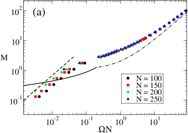
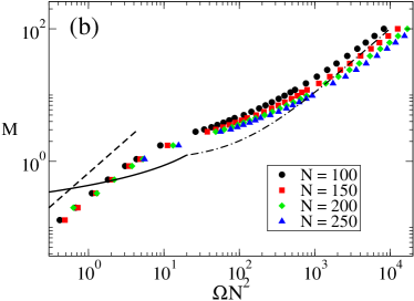
Figure 7: Symbols: Plots of $M$ vs $\Omega N$ (a) and $\Omega N^{1+2\nu}$ (b) as obtained from simulations of ideal polymers ($\nu=1/2$) of various lengths. Dashed and solid lines: analytical predictions from the blob theory ((25), (27) and (32)) for a polymer with length $N=100$. These equations contain no adjustable parameters. (25) and (27) are analytically continued beyond their domain of validity, which produces a crossing of the two lines. In agreement with the blob theory, the simulation data indicate that the torque is a function of the scaling variable $\Omega N^{1+2\nu}$ in the equilibrium regime, while it is a function of $\Omega N$ in the trumpet and stem-trumpet regimes. The standard error, which is in the horizontal direction since $\Omega$ was measured, is smaller than symbol size.

3.3 $\mathbf{M}$ vs. $\boldsymbol{\Omega}$

7 shows a plot of the applied torque $M$ vs. $\Omega N$ (a) and vs. $\Omega N^{1+2\nu}$ (b) as obtained for the simulations for polymers of various lengths (we consider here only the case of ideal polymers ($\nu=1/2$)). The lines are the plots of the blob theory predictions ((25), (27) and (32)) for a polymer of length $N=100$. At low and high torques, the torque is proportional to the angular velocity, which is in agreement with the predictions of (25) and (32). The two regimes are separated by an intermediate (trumpet) regime, where “thinning” occurs: the torque increases more slowly than linear in $\Omega$. In the low torque (equilibrium) regime the data from polymers of various lengths collapse when plotted as function of $\Omega N^{2}$ (7(b)), in agreement with (25). At higher torques the data collapse when plotted as functions of $\Omega N$ (7(a)), which is again in agreement with  (27) and (32). There is an overall quite satisfactory quantitative agreement between theory and simulations, keeping into account that we use no adjustable parameters in (25), (27) and (32) (we used $\tau_{0}=1$ as estimated from our simulations units). Comparing the simulations with the torsional blob theory predictions, we find that the differences are at most within a factor three. We recall that the torque-balance arguments in the blob theory are based on quasi-equalities which ignore unknown numerical prefactors which are expected to be of the order of unity. A more detailed test of the dependence of $M$ on $\Omega$ in the trumpet regime (as predicted by (27)) is at the moment not possible because logarithmic dependences are notoriously difficult to establish as they require very long polymers.

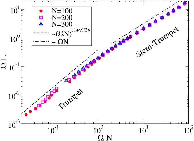
Figure 8: Plot of $\Omega L$ vs. $\Omega N$ for three self-avoiding polymers of different lengths. The elongation $L$, defined in 47 is the distance along the rod axis between the two end monomers. The simulation data agree well with the blob theory, which predicts two different scaling behaviors in the trumpet $\Omega L\sim(\Omega N)^{1.33}$ and in the stem-trumpet $\Omega L\sim\Omega N$ regimes (the Flory exponent for self-avoiding polymers is $\nu\approx 0.588$). The standard error is smaller than symbol size.

3.4 Elongation along the rod

The elongation of the polymer along the rod was computed only for the case of self avoidance where ¹⁰ $\nu\approx 0.588$. In the simulation we determined the average absolute distance between the $z$-coordinates of the first and last monomer, so the elongation is defined as

$$L=\left\langle\left|z(0)-z(N)\right|\right\rangle.$$ (47)

As we are interested in the behavior of $L$ in the trumpet and stem-trumpet regimes we plot in 8 $\Omega L$ vs. $\Omega N$ for polymers of various lengths. For self-avoiding polymers the theoretical prediction (36) implies $\tau_{0}\Omega L\simeq a(\tau_{0}\Omega N)^{1.33}$. In the stem trumpet regime, (37) yields to leading order in $N$: $\tau_{0}\Omega L\simeq h\tau_{0}\Omega N$. The crossover between these two regimes around $\tau_{0}\Omega N\simeq 1$ (19) is indeed observed in 8, where the data belonging to polymers of different lengths collapse into a single curve.

4 Conclusions

In this paper, we gave a full description of the stationary rotation of a flexible polymer induced by a torque. Using a local torque-balance equation, we computed the polymer shape as a function of the curvilinear coordinate $s$. We identify three regimes as the angular velocity increases (or equivalently, when the torque applied to the monomer attached to the rod increases). (i) The equilibrium regime, where the polymer is not perturbed from its equilibrium configuration. (ii) The trumpet regime, in which the polymer is composed of blobs of decreasing size, starting from the free end. Here the blob size decays as $1/\sqrt{s}$, which is much slower than the case of a constant force applied at one end ($\sim 1/s$). Finally (iii) the stem-trumpet regime is defined when a part of the polymer close to the attached monomer is tightly wound around the axis while the free end still displays a trumpet shape.

One of the central results of this paper is the characterization of the response of the total torque $M$ to a change of the angular velocity $\Omega$ or the number of monomers $N$. In the equilibrium and the stem-trumpet regime, the torque is proportional to the angular velocity $M\simeq\Gamma\Omega$. The torque friction, $\Gamma$, has a different scaling behavior with the polymer length in equilibrium $\Gamma\propto N^{1+2\nu}$ compared to the stem-trumpet regime $\Gamma\propto N$. More surprisingly, in the trumpet regime the torque has a very weak (logarithmic) dependence on $\Omega$. This dependence stems from the fact that when the torque is increased the polymer gets closer to the central axis hereby reducing the resistance to the rotational motion. Non-power law, and specifically logarithmic, behavior has already been predicted, simulated and observed in the case of polymer stretching.^{12, 13} However, in that case a situation where both ends are subjected to a force is studied and the logarithmic dependence represents an increase of resistance for high forces due to short-scale DNA crumpling. The setup we consider is different: the resistance decreases in an intermediate torque regime, due to the decrease in distance between the polymer and the rod.

The torque-torsional blob relation (16) is an analogue of the well-known force-tensile blob relation in the pulling problem ¹¹, and is expected to play an essential role to further explore the rotational dynamics. It would be interesting to check experimentally the predictions of the theory. The experimental protocol could be achieved with excitable cylinders in an optical torque wrench ⁴². A polymer could be attached to the cylinder and the other end of the polymer labelled with a fluorescent molecule, allowing, e.g., to test the dependence of spacing of the free end from the axis of rotation with respect to the angular velocity.

5 Acknowledgement

B.B. acknowledges the support of Grant No CA077712 from the National Cancer Institute, NIH to the Hanawalt laboratory at Stanford University. T.S. is supported by KAKENHI [Grant No.26103525, “Fluctuation and Structure”, Grant No.24340100, Grant-in-Aid for Scientific Research (B)], Ministry of Education, Culture, Sports, Science and Technology (MEXT), Japan and JSPS Core-to-Core Program (Nonequilibrium Dynamics of Soft Matter and Information). J-C.W. acknowledges the support by the Laboratory of Excellence Initiative (Labex) NUMEV, OD by the Scientific Council of the University of Montpellier.

Table of Contents graphic

Torque-induced rotational dynamics in polymers: Torsional blobs and thinning

Michiel Laleman, Marco Baiesi, Boris P. Belotserkovskii, Takahiro Sakaue, Jean-Charles Walter and Enrico Carlon

References

- Panja et al. 2013 Panja, D.; Barkema, G. T.; Kolomeisky, A. B. J. Phys.: Condens. Matter 2013, 25, 413101
- Palyulin et al. 2014 Palyulin, V. V.; Ala-Nissila, T.; Metzler, R. Soft Matter 2014, 10, 9016–9037
- Belotserkovskii and Hanawalt 2011 Belotserkovskii, B. P.; Hanawalt, P. C. Biophys. J. 2011, 100, 675–684
- Belotserkovskii 2014 Belotserkovskii, B. P. Phys. Rev. E 2014, 89, 022709
- Liu and Wang 1987 Liu, L.; Wang, J. Proc. Natl. Acad. Sci. 1987, 84, 7024
- Tsao et al. 1989 Tsao, Y.-P.; Wu, H.-Y.; Liu, L. Cell 1989, 56, 111
- Dasanna et al. 2012 Dasanna, A. K.; Destainville, N.; Palmeri, J.; Manghi, M. Europhys. Lett. 2012, 98, 38002
- Dasanna et al. 2013 Dasanna, A. K.; Destainville, N.; Palmeri, J.; Manghi, M. Phys. Rev. E 2013, 87, 052703
- Wada and Netz 2009 Wada, H.; Netz, R. R. Europhys. Lett. 2009, 87, 38001
- de Gennes 1979 de Gennes, P.-G. Scaling Concepts in Polymer Physics; Cornell University Press: Ithaca, USA, 1979
- Pincus 1976 Pincus, P. Macromolecules 1976, 9, 386–388
- Saleh et al. 2009 Saleh, O. A.; McIntosh, D. B.; Pincus, P.; Ribeck, N. Phys. Rev. Lett. 2009, 102, 068301
- Stevens et al. 2013 Stevens, M. J.; McIntosh, D. B.; Saleh, O. A. Macromolecules 2013, 46, 6369–6373
- Nikoofard et al. 2014 Nikoofard, N.; Hoseinpoor, S. M.; Zahedifar, M. Phys. Rev. E 2014, 90, 062603
- Reisner et al. 2005 Reisner, W.; Morton, K. J.; Riehn, R.; Wang, Y. M.; Yu, Z.; Rosen, M.; Sturm, J. C.; Chou, S. Y.; Frey, E.; Austin, R. H. Phys. Rev. Lett. 2005, 94, 196101
- Sakaue and Raphael 2006 Sakaue, T.; Raphael, E. Macromolecules 2006, 39, 2621–2628
- Klushin et al. 2013 Klushin, L. I.; Polotsky, A. A.; Hsu, H.-P.; Markelov, D. A.; Binder, K.; Skvortsov, A. M. Phys. Rev. E 2013, 87, 022604
- Brochard-Wyart 1993 Brochard-Wyart, F. Europhys. Lett. 1993, 23, 105
- Brochard-Wyart et al. 1994 Brochard-Wyart, F.; Hervet, H.; Pincus, P. Europhys. Lett. 1994, 26, 511
- Perkins et al. 1995 Perkins, T. T.; Smith, D. E.; Larson, R. G.; Chu, S. Science 1995, 268, 83–87
- Obermayer et al. 2007 Obermayer, B.; Hallatschek, O.; Frey, E.; Kroy, K. Eur. Phys. J. E 2007, 23, 375–388
- Sakaue et al. 2012 Sakaue, T.; Saito, T.; Wada, H. Phys. Rev. E 2012, 86, 011804
- Rowghanian and Grosberg 2012 Rowghanian, P.; Grosberg, A. Y. Phys. Rev. E 2012, 86, 011803
- Sakaue 2007 Sakaue, T. Phys. Rev. E 2007, 76, 021803
- Frederickx et al. 2014 Frederickx, R.; In’t Veld, T.; Carlon, E. Phys. Rev. Lett. 2014, 112, 198102
- Khorshid et al. 2014 Khorshid, A.; Zimny, P.; Tétreault-La Roche, D.; Massarelli, G.; Sakaue, T.; Reisner, W. Phys. Rev. Lett. 2014, 113, 268104
- Walter et al. 2014 Walter, J.-C.; Baiesi, M.; Carlon, E.; Schiessel, H. Macromolecules 2014, 47, 4840–4846
- Walter et al. 2014 Walter, J.-C.; Laleman, M.; Baiesi, M.; Carlon, E. Eur. Phys. J. Special Topics 2014, 223, 3201–3213
- Walter et al. 2013 Walter, J.-C.; Baiesi, M.; Barkema, G. T.; Carlon, E. Phys. Rev. Lett. 2013, 110, 068301
- Buguin and Brochard-Wyart 1996 Buguin, A.; Brochard-Wyart, F. Macromolecules 1996, 29, 4937–4943
- Brochard-Wyart 1995 Brochard-Wyart, F. Europhys. Lett. 1995, 30, 387
- Fisher et al. 1984 Fisher, M. E.; Privman, V.; Redner, S. J. Phys. A: Math. Gen. 1984, 17, L569
- Rudnick and Hu 1987 Rudnick, J.; Hu, Y. J. Phys. A: Math. Gen. 1987, 20, 4421
- Duplantier and Saleur 1988 Duplantier, B.; Saleur, H. Phys. Rev. Lett. 1988, 60, 2343–2346
- Walter et al. 2011 Walter, J.-C.; Barkema, G. T.; Carlon, E. J. Stat. Mech.: Theory and Exp. 2011, 2011, P10020
- Plimpton 1995 Plimpton, S. J. Comp. Phys. 1995, 117, 1 – 19
- Kremer and Grest 1990 Kremer, K.; Grest, G. S. J. Chem. Phys. 1990, 92, 5057–5086
- Weeks et al. 1971 Weeks, J. D.; Chandler, D.; Andersen, H. C. J. Chem. Phys. 1971, 54, 5237–5247
- Ryckaert et al. 1977 Ryckaert, J.-P.; Ciccotti, G.; Berendsen, H. J. J. Comp. Phys. 1977, 23, 327 – 341
- Schneider and Stoll 1978 Schneider, T.; Stoll, E. Phys. Rev. B 1978, 17, 1302–1322
- Dünweg and Paul 1991 Dünweg, B.; Paul, W. Int. J. Mod. Phys. C 1991, 02, 817–827
- Pedaci et al. 2011 Pedaci, F.; Huang, Z.; van Oene, M.; Barland, S.; Dekker, N. H. Nature Phys. 2011, 7, 259–264