Residual-based a posteriori error estimation for the Maxwell’s eigenvalue problem

Abstract

We present an a posteriori estimator of the error in the $\mathrm{L}^{2}$-norm for the numerical approximation of the Maxwell’s eigenvalue problem by means of Nédélec finite elements. Our analysis is based on a Helmholtz decomposition of the error and on a superconvergence result between the $\mathrm{L}^{2}$-orthogonal projection of the exact eigenfunction onto the curl of the Nédélec finite element space and the eigenfunction approximation. Reliability of the a posteriori error estimator is proved up to higher order terms and local efficiency of the error indicators is shown by using a standard bubble functions technique. The behavior of the a posteriori error estimator is illustrated on a numerical test. A posteriori error estimate, Maxwell’s eigenvalue problem, Nédélec finite elements, mixed formulation

1 Introduction

One of the most classical problems in electromagnetism is the so called cavity problem for Maxwell’s equations, which corresponds to computing the resonant frequencies of a bounded perfectly conducting cavity. This amounts to solving the eigenvalue problem for the Maxwell’s system. Although there has been an intense research in this area, to the best of authors’ knowledge, no results on a posteriori error estimation of Maxwell’s eigenvalue problem are available in the literature.

A posteriori error estimation for various problems involving Maxwell’s equations has been subject of several papers. Residual-based a posteriori error analyses have been done for an electromagnetic scattering problem in Monk (1998) and for an eddy current problem in Beck et al. (2000); in both cases, smooth coefficients and sufficiently regular domains have been considered. Generalizations to piecewise constant coefficients and to Lipschitz domains have been done in Nicaise & Creusé (2003) and Schöberl (2008), respectively. Estimates robust with respect to the coefficients of the equations have been obtained in Cochez-Dhondt & Nicaise (2007). The $hp$-version has been considered in Bürg (2011, 2012), where bounds with explicit dependence on the polynomial degree have been derived. Further, convergence of an $hp$-adaptive strategy based on these estimates has been studied in Bürg (2013). Residual-based a posteriori error estimates have been also obtained for the $\bm{A}-\phi$ and the $\bm{T}/\Omega$ magnetodynamic harmonic formulations in Creusé et al. (2012) and Creusé et al. (2013), respectively, and for the time-harmonic Maxwell’s equations with strong singularities in Chen et al. (2007). Functional-type error estimates for the time-harmonic Maxwell’s equations have been derived in Repin (2007) and Hannukainen (2008). A drawback of this approach is that it requires to solve a global auxiliary problem. By contrast, equilibrated fluxes-based a posteriori error estimates requiring to solve only local problems have been analyzed in Braess & Schöberl (2008). Furthermore, implicit error estimates have been derived in Harutyunyan et al. (2008) and a Zienkiewicz–Zhu error estimator based on a patch recovery has been introduced in Nicaise (2005).

On the other hand, a posteriori error estimation for different spectral problems has been subject of several papers, too. Among the first ones, we mention Verfürth (1994); Larson (2000); Durán et al. (2003) for the standard finite element approximation of second-order elliptic eigenvalue problems. We also mention Garau et al. (2009) and Giani & Graham (2009), where adaptive schemes based on this estimators have been proved to converge.

In its turn, the first paper dealing with a posteriori error estimates for a mixed formulation of an eigenvalue problem seems to be Durán et al. (1999), where Raviart–Thomas finite elements are used for the discretization of the spectral problem for the Laplace operator. The analysis in this reference makes use of a Helmholtz decomposition of the error, as is typical in the a posteriori error analysis of mixed problems. It also uses a superconvergent approximation of the primal variable, which is constructed by exploiting the equivalency between the lowest-order Raviart–Thomas mixed discretization and a non-conforming method for the primal problem based on the Crouzeix–Raviart space enriched by bubble functions. This approach has been extended to fluid-structure vibration problems in Alonso et al. (2001, 2004). However, in spite of many existing analogies, a direct extension of these ideas to Maxwell’s eigenvalue problem does not seem feasible, because no element that could play the role of Crouzeix–Raviart’s in Durán et al. (1999) is known.

An alternative analysis which avoids the relation between Raviart–Thomas and Crouzeix–Raviart elements has been more recently explored in (Boffi et al., 2012, Section 6.4.2). The results from this reference are based on a superconvergence result from Gardini (2009). A similar result is obtained in Lin & Xie (2012) for more general second-order elliptic eigenvalue problems and mixed finite element methods. In both cases, an interpolation coming from the commuting diagram applied to the primal variable comes to play a role in order to prove superconvergence with respect to the eigenfunction approximation. An a posteriori error estimator based on this result has been proposed in Jia et al. (2013). More recently, a similar analysis has been used to conclude convergence of an adaptive scheme in Boffi et al. (2015).

We derive in this paper a posteriori error estimates of the error in the $\mathrm{L}^{2}$-norm for the Maxwell’s eigenvalue problem discretized by Nédélec elements (see Boffi et al. (1999); Boffi (2000); Caorsi et al. (2000); Monk & Demkowicz (2001) for the a priori analysis). With this end, we adapt the results from Durán et al. (1999); Boffi et al. (2012); Lin & Xie (2012); Jia et al. (2013). However, our approach use neither an alternative discretization (as in Durán et al. (1999)) nor an interpolation coming from the commuting diagram (as in the other references) for obtaining a superconvergence approximation of the primal variable. Instead, we use a superconvergence result between the $\mathrm{L}^{2}$-orthogonal projection of the eigenfunction onto the curl of the Nédélec finite element space and the eigenfunction approximation.

The structure of the paper is the following. We introduce primal and mixed weak formulations of the Maxwell’s eigenvalue problem and their corresponding finite element discretizations in Section 2. The superconvergence result is established in Section 3. A posteriori error estimates in the $\mathrm{L}^{2}$-norm are derived and reliability and local efficiency of the error indicators are proved in Section 4. The paper is concluded with Section 5, where the behavior of the derived estimates is illustrated on a numerical test.

2 Continuous and discrete problems

In this section we introduce continuous and discrete variational formulations of the problem under interest.

2.1 Preliminaries

Let $\Omega\subset\mathbb{R}^{3}$ be a domain with polyhedral Lipschitz boundary $\partial\Omega$. For the sake of simplicity, we assume that $\Omega$ is non-convex and simply-connected and that its boundary is connected. Let $\bm{n}$ be the unit outward normal to $\partial\Omega$.

We use standard notation for Lebesgue and Sobolev spaces. Specifically, for a given domain $M\subset\mathbb{R}^{3}$, $\mathrm{L}^{2}(M)$ denotes the space of square-integrable functions and, for $t\in\mathbb{N}$, $\mathrm{H}^{t}(M)$ denotes the space of functions having square-integrable weak derivatives up to the $t$-th order. For $t\notin\mathbb{N}$ ($t>0$), $\mathrm{H}^{t}(M)$ denotes the standard fractional Sobolev space. For any $t>0$, $\left\|\cdot\right\|_{t,M}$ denotes the norm of the Sobolev space $\mathrm{H}^{t}(M)$. We recall that for any $t>0$ the inclusion $\mathrm{H}^{t}(M)\hookrightarrow\mathrm{L}^{2}(M)$ is compact. We also denote $\mathbf{L}^{2}(M):=[\mathrm{L}^{2}(M)]^{3}$ and $\mathbf{H}^{t}(M):=[\mathrm{H}^{t}(M)]^{3}$. Further, $\left(\cdot,\cdot\right)_{M}$ denotes the inner product in $\mathrm{L}^{2}(M)$ or $\mathbf{L}^{2}(M)$ and $\left\|\cdot\right\|_{0,M}$ the induced norm. Analogously, $\left(\cdot,\cdot\right)_{\partial M}$ denotes the $(d-1)$-dimensional $\mathrm{L}^{2}(\partial M)$ inner product; the same notation is applied in the vector case. We will omit subscript $M$ in case $M=\Omega$.

We denote by $C$ a generic positive constant, not necessarily the same at each occurrence, but always independent of the mesh refinement parameter $h$ which will be introduced in the next subsection.

We recall the definition of some classical spaces that will be used in the sequel:

$$\mathrm{H}^{1}_{0}(\Omega) :=\left\{v\in\mathrm{H}^{1}(\Omega):\ v=0\ \ \text{on }\partial\Omega\right\};$$

$$\mathbf{H}(\operatorname{\mathrm{div}},\Omega) :=\left\{\bm{v}\in\mathbf{L}^{2}(\Omega):\ \operatorname{\mathrm{div}}\bm{v}\in\mathrm{L}^{2}(\Omega)\right\};$$

$$\mathbf{H}_{0}(\operatorname{\mathrm{div}},\Omega) :=\left\{\bm{v}\in\mathbf{H}(\operatorname{\mathrm{div}},\Omega):\ \bm{v}\cdot\bm{n}=0\ \ \text{on }\partial\Omega\right\};$$

$$\mathbf{H}(\operatorname{\mathrm{div}}^{0},\Omega) :=\left\{\bm{v}\in\mathbf{H}(\operatorname{\mathrm{div}},\Omega):\ \operatorname{\mathrm{div}}\bm{v}=0\ \ \text{in }\Omega\right\};$$

$$\mathbf{H}_{0}(\operatorname{\mathrm{div}}^{0},\Omega) :=\mathbf{H}_{0}(\operatorname{\mathrm{div}},\Omega)\cap\mathbf{H}(\operatorname{\mathrm{div}}^{0},\Omega);$$

$$\mathbf{H}(\operatorname{\mathbf{curl}},\Omega) :=\left\{\bm{v}\in\mathbf{L}^{2}(\Omega):\ \operatorname{\mathbf{curl}}\bm{v}\in\mathbf{L}^{2}(\Omega)\right\};$$

$$\mathbf{H}_{0}(\operatorname{\mathbf{curl}},\Omega) :=\left\{\bm{v}\in\mathbf{H}(\operatorname{\mathbf{curl}},\Omega):\ \bm{v}\times\bm{n}=\bm{0}\ \ \text{on }\partial\Omega\right\};$$

$$\mathbf{H}(\operatorname{\mathbf{curl}}^{0},\Omega) :=\left\{\bm{v}\in\mathbf{H}(\operatorname{\mathbf{curl}},\Omega):\ \operatorname{\mathbf{curl}}\bm{v}=\bm{0}\ \ \text{in }\Omega\right\};$$

$$\mathbf{H}_{0}(\operatorname{\mathbf{curl}}^{0},\Omega) :=\mathbf{H}_{0}(\operatorname{\mathbf{curl}},\Omega)\cap\mathbf{H}(\operatorname{\mathbf{curl}}^{0},\Omega);$$

$$\mathbf{H}^{t}(\operatorname{\mathbf{curl}},\Omega) :=\left\{\bm{v}\in\mathbf{H}^{t}(\Omega):\ \operatorname{\mathbf{curl}}\bm{v}\in\mathbf{H}^{t}(\Omega)\right\}\quad(t>0).$$

Spaces $\mathbf{H}(\operatorname{\mathrm{div}},\Omega)$ and $\mathbf{H}(\operatorname{\mathbf{curl}},\Omega)$ endowed with the norms defined by

$$\left\|\bm{v}\right\|_{\operatorname{\mathrm{div}}}^{2}:=\left\|\bm{v}\right\|_{0}^{2}+\left\|\operatorname{\mathrm{div}}\bm{v}\right\|_{0}^{2}\qquad\text{and}\qquad\left\|\bm{v}\right\|_{\operatorname{\mathbf{curl}}}^{2}:=\left\|\bm{v}\right\|_{0}^{2}+\left\|\operatorname{\mathbf{curl}}\bm{v}\right\|_{0}^{2},$$

respectively, are Hilbert spaces. In turn, $\mathbf{H}_{0}(\operatorname{\mathrm{div}},\Omega)$, $\mathbf{H}(\operatorname{\mathrm{div}}^{0},\Omega)$ and $\mathbf{H}_{0}(\operatorname{\mathrm{div}}^{0},\Omega)$ are closed subspaces of $\mathbf{H}(\operatorname{\mathrm{div}},\Omega)$. In its turn, $\mathbf{H}_{0}(\operatorname{\mathbf{curl}},\Omega)$, $\mathbf{H}(\operatorname{\mathbf{curl}}^{0},\Omega)$ and $\mathbf{H}_{0}(\operatorname{\mathbf{curl}}^{0},\Omega)$ are closed subspaces of $\mathbf{H}(\operatorname{\mathbf{curl}},\Omega)$.

We also denote

$$\bm{\mathcal{M}}:=\operatorname{\mathbf{curl}}(\mathbf{H}_{0}(\operatorname{\mathbf{curl}},\Omega))$$

endowed with the $\mathbf{L}^{2}(\Omega)$-norm. Notice that $\bm{\mathcal{M}}=\mathbf{H}_{0}(\operatorname{\mathrm{div}}^{0},\Omega)$ (see Amrouche et al. (1998)), which is a Hilbert space.

In the paper we will repeatedly use the following embedding theorem.

Theorem 2.1.

There exists $t\in\left(\frac{1}{2},1\right)$ such that the following inclusions are continuous:

$$\left.\begin{array}[]{rc}\mathbf{H}_{0}(\operatorname{\mathbf{curl}},\Omega)\cap\mathbf{H}(\operatorname{\mathrm{div}},\Omega)\\[2.84544pt] \mathbf{H}(\operatorname{\mathbf{curl}},\Omega)\cap\mathbf{H}_{0}(\operatorname{\mathrm{div}},\Omega)\end{array}\right\}\hookrightarrow\mathbf{H}^{t}(\Omega).$$

Moreover, there exists $C>0$ such that

$$\left\|\bm{v}\right\|_{t}\leq C\left(\left\|\operatorname{\mathbf{curl}}\bm{v}\right\|_{0}+\left\|\operatorname{\mathrm{div}}\bm{v}\right\|_{0}\right)$$

for all $\bm{v}\in\mathbf{H}_{0}(\operatorname{\mathbf{curl}},\Omega)\cap\mathbf{H}(\operatorname{\mathrm{div}},\Omega)$ or $\bm{v}\in\mathbf{H}(\operatorname{\mathbf{curl}},\Omega)\cap\mathbf{H}_{0}(\operatorname{\mathrm{div}},\Omega)$.

Proof 2.2.

The inclusions in $\mathbf{H}^{t}(\Omega)$ with $t>1/2$ can be found in (Amrouche et al., 1998, Proposition 3.7), for instance; the constraint $t<1$ comes from the fact that $\Omega$ is not convex. The estimate follows from (Amrouche et al., 1998, Corollary 3.16) and the simple connectedness of $\Omega$ for $\bm{v}\in\mathbf{H}(\operatorname{\mathbf{curl}},\Omega)\cap\mathbf{H}_{0}(\operatorname{\mathrm{div}},\Omega)$ and from (Amrouche et al., 1998, Corollary 3.19) and the fact that $\partial\Omega$ is connected for $\bm{v}\in\mathbf{H}_{0}(\operatorname{\mathbf{curl}},\Omega)\cap\mathbf{H}(\operatorname{\mathrm{div}},\Omega)$.

2.2 Continuous problem

In a homogeneous and isotropic medium, by setting all the physical constants to 1, the Maxwell’s eigenvalue problem reduces to finding $\lambda\in\mathbb{R}$ and $\bm{u}:\,\Omega\longrightarrow\mathbb{R}^{3}$, $\bm{u}\neq\bm{0}$, satisfying

$$\operatorname{\mathbf{curl}}(\operatorname{\mathbf{curl}}\bm{u}) =\lambda\bm{u}\quad\text{in }\Omega,$$

$$\operatorname{\mathrm{div}}\bm{u} =0\quad\text{in }\Omega,$$

$$\bm{u}\times\bm{n} =\bm{0}\quad\text{on }\partial\Omega.$$

We will consider two formulations of this problem, one primal and the other mixed. In order to make the numerical approximation easier, the former usually drops the divergence free constraint. Then, the primal formulation reads as follows.

Problem 2.3.

Find $\left(\lambda,\bm{u}\right)\in\mathbb{R}\times\mathbf{H}_{0}(\operatorname{\mathbf{curl}},\Omega)$, $\bm{u}\neq\bm{0}$, such that

$$\left(\operatorname{\mathbf{curl}}\bm{u},\operatorname{\mathbf{curl}}\bm{v}\right)=\lambda\left(\bm{u},\bm{v}\right)\qquad\forall\bm{v}\in\mathbf{H}_{0}(\operatorname{\mathbf{curl}},\Omega).$$

The eigenvalues of this problem consist of $\lambda=0$ with eigenspace $\mathbf{H}_{0}(\operatorname{\mathbf{curl}}^{0},\Omega)=\nabla(\mathrm{H}^{1}_{0}(\Omega))$ and a sequence of positive real numbers $\left\{\lambda_{n}\right\}_{n=1}^{\infty}$ which satisfy $\lambda_{n}\to\infty$.

For $\lambda\neq 0$, by introducing $\bm{\sigma}:=\left(\operatorname{\mathbf{curl}}\bm{u}\right)/\lambda\in\bm{\mathcal{M}}$, we are led to the following mixed formulation.

Problem 2.4.

Find $\left(\lambda,\bm{u},\bm{\sigma}\right)\in\mathbb{R}\times\mathbf{H}_{0}(\operatorname{\mathbf{curl}},\Omega)\times\bm{\mathcal{M}}$, $\left(\bm{u},\bm{\sigma}\right)\neq\bm{0}$, such that

$$\left(\bm{u},\bm{v}\right)-\left(\operatorname{\mathbf{curl}}\bm{v},\bm{\sigma}\right)=0 \qquad\forall\bm{v}\in\mathbf{H}_{0}(\operatorname{\mathbf{curl}},\Omega),$$ (2.1a)

$$-\left(\operatorname{\mathbf{curl}}\bm{u},\bm{\tau}\right)=-\lambda\left(\bm{\sigma},\bm{\tau}\right) \qquad\forall\bm{\tau}\in\bm{\mathcal{M}}.$$ (2.1b)

The spectra of Problems 2.3 and 2.4 are identical, except for $\lambda=0$ which is not an eigenvalue of the latter. More precisely, both problems are equivalent for $\lambda\neq 0$ in the following sense:

• if $\left(\lambda,\bm{u}\right)$ is an eigenpair of Problem 2.3 with $\lambda\neq 0$, then $\left(\lambda,\bm{u},\frac{1}{\lambda}\operatorname{\mathbf{curl}}\bm{u}\right)$ is a solution of Problem 2.4;

• if $\left(\lambda,\bm{u},\bm{\sigma}\right)$ is a solution of Problem 2.4, then $\left(\lambda,\bm{u}\right)$ is a solution of Problem 2.3 and $\bm{\sigma}=\frac{1}{\lambda}\left(\operatorname{\mathbf{curl}}\bm{u}\right)$.

For the purpose of subsequent analysis, we define the solution operators

$$\bm{T}:\;\bm{\mathcal{M}}\longrightarrow\bm{\mathcal{M}}\qquad\text{and}\qquad\bm{S}:\;\bm{\mathcal{M}}\longrightarrow\mathbf{H}_{0}(\operatorname{\mathbf{curl}},\Omega)$$

as follows: given $\bm{g}\in\bm{\mathcal{M}}$, $(\bm{S}\bm{g},\bm{T}\bm{g})\in\mathbf{H}_{0}(\operatorname{\mathbf{curl}},\Omega)\times\bm{\mathcal{M}}$ is the solution of

$$\left(\bm{S}\bm{g},\bm{v}\right)-\left(\operatorname{\mathbf{curl}}\bm{v},\bm{T}\bm{g}\right)=0 \qquad\forall\bm{v}\in\mathbf{H}_{0}(\operatorname{\mathbf{curl}},\Omega),$$ (2.2a)

$$-\left(\operatorname{\mathbf{curl}}(\bm{S}\bm{g}),\bm{\tau}\right)=-\left(\bm{g},\bm{\tau}\right) \qquad\forall\bm{\tau}\in\bm{\mathcal{M}}.$$ (2.2b)

Lemma 2.5.

Equations (2.2) yield a well-posed problem.

Proof 2.6.

We define $a(\bm{u},\bm{v}):=\left(\bm{u},\bm{v}\right)$ for $\bm{u},\bm{v}\in\mathbf{H}_{0}(\operatorname{\mathbf{curl}},\Omega)$ and $b(\bm{v},\bm{\tau}):=\left(\operatorname{\mathbf{curl}}\bm{v},\bm{\tau}\right)$ for $\bm{v}\in\mathbf{H}_{0}(\operatorname{\mathbf{curl}},\Omega)$ and $\bm{\tau}\in\bm{\mathcal{M}}$. According to the classical theory for mixed finite element methods (see, e.g., Boffi et al. (2013)), it is enough to prove the ellipticity of $a$ in the kernel of $b$ and the inf-sup condition for $b$ for the problem to be well-posed.

The kernel of $b$ has the form

$$\bm{\mathcal{K}}:=\left\{\bm{v}\in\mathbf{H}_{0}(\operatorname{\mathbf{curl}},\Omega):\ \left(\bm{\tau},\operatorname{\mathbf{curl}}\bm{v}\right)=0\ \ \forall\bm{\tau}\in\bm{\mathcal{M}}\right\}=\mathbf{H}_{0}(\operatorname{\mathbf{curl}}^{0},\Omega),$$

so that the ellipticity of $a$ in the kernel of $b$ follows immediately:

$$a(\bm{v},\bm{v})=\left\|\bm{v}\right\|^{2}_{0}=\left\|\bm{v}\right\|^{2}_{\operatorname{\mathbf{curl}}}\qquad\forall\bm{v}\in\bm{\mathcal{K}}.$$

On the other hand, let $\bm{\tau}\in\bm{\mathcal{M}}$ be arbitrary but fixed. Since $\bm{\mathcal{M}}=\mathbf{H}_{0}(\operatorname{\mathrm{div}}^{0},\Omega)$, due to (Amrouche et al., 1998, Therorem 3.17), there exists a vector potential $\bm{v}_{\bm{\tau}}\in\mathbf{H}_{0}(\operatorname{\mathbf{curl}},\Omega)\cap\mathbf{H}(\operatorname{\mathrm{div}}^{0},\Omega)$ of $\bm{\tau}$, such that $\operatorname{\mathbf{curl}}\bm{v}_{\bm{\tau}}=\bm{\tau}$ and $\left\|\bm{v}_{\bm{\tau}}\right\|_{\operatorname{\mathbf{curl}}}\leq C\left\|\bm{\tau}\right\|_{0}$ (see (Amrouche et al., 1998, Corollary 3.19)). Consequently, by taking $\bm{v}:=\bm{v}_{\bm{\tau}}$ in the supremum below, we obtain

$$\sup_{\bm{v}\in\mathbf{H}_{0}(\operatorname{\mathbf{curl}},\Omega)}\frac{\left(\bm{\tau},\operatorname{\mathbf{curl}}\bm{v}\right)}{\left\|\bm{v}\right\|_{\operatorname{\mathbf{curl}}}}\geq\frac{\left\|\bm{\tau}\right\|^{2}_{0}}{\left\|\bm{v}_{\bm{\tau}}\right\|_{\operatorname{\mathbf{curl}}}}\geq\frac{1}{C}\left\|\bm{\tau}\right\|_{0}.$$

Since $\bm{\tau}\in\bm{\mathcal{M}}$ has been chosen arbitrarily, we derive the inf-sup condition for $b$, which together with the ellipticity of $a$ in the kernel of $b$ allow us to conclude that the mixed formulation (2.2) is well-posed.

In the following lemma we derive some additional regularity for $\bm{S}\bm{g}$ and $\bm{T}\bm{g}$, which will yield additional regularity for the solutions of the eigenvalue problem as well.

Lemma 2.7.

For all $\bm{g}\in\bm{\mathcal{M}}$, $\bm{S}\bm{g}=\operatorname{\mathbf{curl}}(\bm{T}\bm{g})$. Moreover, $\bm{T}\bm{g}$ and $\bm{S}\bm{g}$ both belong to $\mathbf{H}^{t}(\Omega)$ with $t\in\left(\frac{1}{2},1\right)$ as in Theorem 2.1 and

$$\left\|\bm{S}\bm{g}\right\|_{t}+\left\|\bm{T}\bm{g}\right\|_{t}\leq C\left\|\bm{g}\right\|_{0}.$$

Proof 2.8.

The equality $\bm{S}\bm{g}=\operatorname{\mathbf{curl}}(\bm{T}\bm{g})$ follows from (2.2a) by taking $\bm{v}\in\mathcal{D}(\Omega)^{3}$. Then, $\bm{T}\bm{g}\in\mathbf{H}(\operatorname{\mathbf{curl}},\Omega)\cap\mathbf{H}_{0}(\operatorname{\mathrm{div}}^{0},\Omega)\hookrightarrow\mathbf{H}^{t}(\Omega)$ with $1/2<t<1$ (cf. Theorem 2.1) and

$$\left\|\bm{T}\bm{g}\right\|_{t}\leq C\left\|\operatorname{\mathbf{curl}}(\bm{T}\bm{g})\right\|_{0}=C\left\|\bm{S}\bm{g}\right\|_{0}\leq C\left\|\bm{g}\right\|_{0},$$

where the last inequality holds because of the well-posedness proved in Lemma 2.5. On the other hand, since $\bm{S}\bm{g}=\operatorname{\mathbf{curl}}(\bm{T}\bm{g})$, $\bm{S}\bm{g}\in\mathbf{H}(\operatorname{\mathrm{div}}^{0},\Omega)\cap\mathbf{H}_{0}(\operatorname{\mathbf{curl}},\Omega)\hookrightarrow\mathbf{H}^{t}(\Omega)$ (cf. Theorem 2.1, again) and

$$\left\|\bm{S}\bm{g}\right\|_{t}\leq C\left\|\bm{S}\bm{g}\right\|_{\operatorname{\mathbf{curl}}}\leq C\left\|\bm{g}\right\|_{0},$$

once more because of Lemma 2.5. Thus, we conclude the proof.

Corollary 2.9.

Let $\left(\lambda,\bm{u},\bm{\sigma}\right)$ be a solution of Problem 2.4. Then,

$$\bm{u}=\operatorname{\mathbf{curl}}\bm{\sigma}\quad\text{and}\quad\operatorname{\mathbf{curl}}\bm{u}=\lambda\bm{\sigma}\quad\text{in }\Omega.$$ (2.3)

Moreover, $\bm{u},\bm{\sigma}\in\mathbf{H}^{t}(\operatorname{\mathbf{curl}},\Omega)$ and

$$\left\|\bm{u}\right\|_{t}+\left\|\operatorname{\mathbf{curl}}\bm{u}\right\|_{t}+\left\|\bm{\sigma}\right\|_{t}+\left\|\operatorname{\mathbf{curl}}\bm{\sigma}\right\|_{t}\leq C\left\|\bm{\sigma}\right\|_{0}$$

with $1/2<t<1$ as in Theorem 2.1.

Proof 2.10.

Since $\bm{u}=\bm{S}(\lambda\bm{\sigma})$ and $\bm{\sigma}=\bm{T}(\lambda\bm{\sigma})$, due to the previous lemma, $\bm{u}=\operatorname{\mathbf{curl}}\bm{\sigma}$. Moreover, since $\operatorname{\mathbf{curl}}\bm{u}-\lambda\bm{\sigma}\in\bm{\mathcal{M}}$, equation (2.1b) implies that $\operatorname{\mathbf{curl}}\bm{u}=\lambda\bm{\sigma}$. The rest of the results follow from Lemma 2.7.

2.3 Finite element spaces

We set up the notation for introducing finite element approximations of Problems 2.3 and 2.4. We consider a regular family $\left\{\mathcal{T}_{h}\right\}$ of partitions of the closure of $\Omega$ into a finite number of tetrahedra $K$. As usual, $h:=\max_{K\in\mathcal{T}_{h}}h_{K}$, where $h_{S}$ denotes the diameter of $S$, for any $S\subset\Omega$. We denote by $\mathbb{P}_{k}(K)$ the space of polynomials of degree at most $k$ on $K$ and by $\tilde{\mathbb{P}}_{k}(K)$ the subspace of homogeneous polynomials of degree $k$.

We consider the Nédélec space of order $k$,

$$\bm{\mathcal{N}}_{h}^{\,0}(\Omega):=\left\{\bm{v}_{h}\in\mathbf{H}_{0}(\operatorname{\mathbf{curl}},\Omega):\ \bm{v}_{h}|_{K}\in{[\mathbb{P}_{k}(K)]}^{3}\oplus\bm{x}\times{[\tilde{\mathbb{P}}_{k}(K)]}^{3}\ \ \forall K\in\mathcal{T}_{h}\right\},$$

the Raviart–Thomas space of order $k$,

$$\bm{\mathcal{RT}}_{h}^{\,0}(\Omega):=\left\{\bm{v}_{h}\in\mathbf{H}_{0}(\operatorname{\mathrm{div}},\Omega):\ \bm{v}_{h}|_{K}\in{[\mathbb{P}_{k}(K)]}^{3}\oplus\bm{x}\tilde{\mathbb{P}}_{k}(K)\ \ \forall K\in\mathcal{T}_{h}\right\},$$

the Lagrangian finite element space of order $k$,

$$\mathcal{L}_{h}^{0}(\Omega):=\left\{v_{h}\in\mathcal{C}(\bar{\Omega}):\ v_{h}|_{K}\in\mathbb{P}_{k}(K)\ \ \forall K\in\mathcal{T}_{h}\text{ and }v_{h}=0\text{ on }\partial\Omega\right\}\subset\mathrm{H}^{1}_{0}(\Omega),$$

and the curl of the Nédélec space

$$\bm{\mathcal{M}}_{h}:=\operatorname{\mathbf{curl}}(\bm{\mathcal{N}}_{h}^{\,0}(\Omega)).$$

We will use different interpolants on each of these discrete spaces. In $\mathbf{H}_{0}(\operatorname{\mathbf{curl}},\Omega)$ we will use the Nédélec interpolant,

$$\bm{\mathcal{I}}_{\rm N}:\;\mathbf{H}^{t}(\operatorname{\mathbf{curl}},\Omega)\cap\mathbf{H}_{0}(\operatorname{\mathbf{curl}},\Omega)\longrightarrow\bm{\mathcal{N}}_{h}^{\,0}(\Omega),$$

which is well-defined provided $t>1/2$. In such a case, we have the following interpolation error estimate (see (Monk, 2003, Theorem 5.41(1))):

$$\left\|\bm{v}-\bm{\mathcal{I}}_{\rm N}\bm{v}\right\|_{\operatorname{\mathbf{curl}}}\leq Ch^{\min\{t,k+1\}}\left(\left\|\bm{v}\right\|_{t}+\left\|\operatorname{\mathbf{curl}}\bm{v}\right\|_{t}\right).$$ (2.4)

The Nédélec interpolant is also well-defined for $\bm{v}\in\mathbf{H}^{t}(\Omega)$ with $1/2<t\leq 1$, whenever $\operatorname{\mathbf{curl}}\bm{v}\in\bm{\mathcal{RT}}_{h}^{\,0}(\Omega)$. In such a case, $\operatorname{\mathbf{curl}}(\bm{\mathcal{I}}_{\rm N}\bm{v})=\operatorname{\mathbf{curl}}\bm{v}$ and we have the following error estimate (see (Monk, 2003, Theorem 5.41(2))):

$$\left\|\bm{v}-\bm{\mathcal{I}}_{\rm N}\bm{v}\right\|_{0}\leq C\left(h^{t}\left\|\bm{v}\right\|_{t}+h\left\|\operatorname{\mathbf{curl}}\bm{v}\right\|_{0}\right).$$ (2.5)

In $\mathbf{H}_{0}(\operatorname{\mathrm{div}},\Omega)$ we will use the Raviart–Thomas interpolant,

$$\bm{\mathcal{I}}_{\rm R}:\;\mathbf{H}^{t}(\Omega)\cap\mathbf{H}_{0}(\operatorname{\mathrm{div}},\Omega)\longrightarrow\bm{\mathcal{RT}}_{h}^{\,0}(\Omega),$$

which is well-defined provided $t>0$. In case $t>1/2$, the following error estimate holds true (see (Monk, 2003, Theorem 5.25)):

$$\left\|\bm{v}-\bm{\mathcal{I}}_{\rm R}\bm{v}\right\|_{0}\leq Ch^{\min\{t,k+1\}}\left\|\bm{v}\right\|_{t}.$$ (2.6)

Moreover, it is well-known that for $\bm{v}\in\mathbf{H}^{t}(\Omega)$

$$\operatorname{\mathrm{div}}\bm{v}=0\quad\Rightarrow\quad\operatorname{\mathrm{div}}(\bm{\mathcal{I}}_{\rm R}\bm{v})=0$$ (2.7)

and, for $\bm{v}\in\mathbf{H}^{t}(\operatorname{\mathbf{curl}},\Omega)$,

$$\operatorname{\mathbf{curl}}(\bm{\mathcal{I}}_{\rm N}\bm{v})=\bm{\mathcal{I}}_{\rm R}(\operatorname{\mathbf{curl}}\bm{v});$$ (2.8)

therefore, $\bm{\mathcal{I}}_{\rm R}(\operatorname{\mathbf{curl}}\bm{v})\in\bm{\mathcal{M}}_{h}$.

The following result will be used in the sequel.

Lemma 2.11.

For $\Omega$ simply connected,

$$\operatorname{\mathbf{curl}}(\bm{\mathcal{N}}_{h}^{\,0}(\Omega))=\bm{\mathcal{RT}}_{h}^{\,0}(\Omega)\cap\mathbf{H}(\operatorname{\mathrm{div}}^{0},\Omega).$$

Moreover, there exists $C>0$ (independent of $h$) such that, for all $\bm{\tau}_{h}\in\bm{\mathcal{RT}}_{h}^{\,0}(\Omega)\cap\mathbf{H}(\operatorname{\mathrm{div}}^{0},\Omega)$, there exists $\bm{v}_{h}\in\bm{\mathcal{N}}_{h}^{\,0}(\Omega)$ that satisfies $\operatorname{\mathbf{curl}}\bm{v}_{h}=\bm{\tau}_{h}$ and

$$\left\|\bm{v}_{h}\right\|_{\operatorname{\mathbf{curl}}}\leq C\left\|\bm{\tau}_{h}\right\|_{0}.$$

Proof 2.12.

The inclusion $\operatorname{\mathbf{curl}}(\bm{\mathcal{N}}_{h}^{\,0}(\Omega))\subset\bm{\mathcal{RT}}_{h}^{\,0}(\Omega)\cap\mathbf{H}(\operatorname{\mathrm{div}}^{0},\Omega)$ is well-known (see (Monk, 2003, Lemma 5.40)). To prove the other inclusion, let $\bm{\tau}_{h}\in\bm{\mathcal{RT}}_{h}^{\,0}(\Omega)\cap\mathbf{H}(\operatorname{\mathrm{div}}^{0},\Omega)$. Since $\Omega$ is simply connected, there exists $\bm{v}\in\mathbf{H}_{0}(\operatorname{\mathbf{curl}},\Omega)\cap\mathbf{H}(\operatorname{\mathrm{div}}^{0},\Omega)$ such that $\bm{\tau}_{h}=\operatorname{\mathbf{curl}}\bm{v}$ in $\Omega$ (see (Amrouche et al., 1998, Theorem 3.17)). Then, there exists $t\in\left(\frac{1}{2},1\right)$ such that $\bm{v}\in\mathbf{H}^{t}(\Omega)$ (cf. Theorem 2.1) and $\operatorname{\mathbf{curl}}\bm{v}\in\bm{\mathcal{RT}}_{h}^{\,0}(\Omega)$. Hence, as mentioned above, its Nédélec interpolant $\bm{\mathcal{I}}_{\rm N}\bm{v}\in\bm{\mathcal{N}}_{h}^{\,0}(\Omega)$ is well-defined, $\operatorname{\mathbf{curl}}(\bm{\mathcal{I}}_{\rm N}\bm{v})=\operatorname{\mathbf{curl}}\bm{v}=\bm{\tau}_{h}$ in $\Omega$ and (2.5) holds true. Therefore, $\bm{\tau}_{h}\in\operatorname{\mathbf{curl}}(\bm{\mathcal{N}}_{h}^{\,0}(\Omega))$. Moreover, as a consequence of (2.5) we have that

$$\left\|\bm{\mathcal{I}}_{\rm N}\bm{v}\right\|_{0}\leq\left\|\bm{v}\right\|_{0}+C\left(h^{t}\left\|\bm{v}\right\|_{t}+h\left\|\operatorname{\mathbf{curl}}\bm{v}\right\|_{0}\right)\leq C\left\|\operatorname{\mathbf{curl}}\bm{v}\right\|_{0}=C\left\|\bm{\tau}_{h}\right\|_{0},$$

where we have used Theorem 2.1 for the last inequality. Thus, since $\operatorname{\mathbf{curl}}(\bm{\mathcal{I}}_{\rm N}\bm{v})=\bm{\tau}_{h}$, we conclude the proof by taking $\bm{v}_{h}:=\bm{\mathcal{I}}_{\rm N}\bm{v}$.

2.4 Discrete problem

The finite element approximation of the primal formulation in Problem 2.3 reads as follows.

Problem 2.13.

Find $\left(\lambda_{h},\bm{u}_{h}\right)\in\mathbb{R}\times\bm{\mathcal{N}}_{h}^{\,0}(\Omega)$, $\bm{u}_{h}\neq\bm{0}$, such that

$$\left(\operatorname{\mathbf{curl}}\bm{u}_{h},\operatorname{\mathbf{curl}}\bm{v}_{h}\right)=\lambda_{h}\left(\bm{u}_{h},\bm{v}_{h}\right)\quad\forall\bm{v}_{h}\in\bm{\mathcal{N}}_{h}^{\,0}(\Omega).$$

The eigenvalues of this problem consist of $\lambda_{h}=0$ with corresponding eigenspace $\nabla(\mathcal{L}_{h}^{0}(\Omega))$ and $\lambda_{h,n}>0$, $n=1,\ldots,\operatorname{\mathrm{dim}}(\bm{\mathcal{N}}_{h}^{\,0}(\Omega))-\operatorname{\mathrm{dim}}(\mathcal{L}_{h}^{0}(\Omega))+1$.

In turn, the finite element approximation of the mixed formulation in Problem 2.4 is the following.

Problem 2.14.

Find $\left(\lambda_{h},\bm{u}_{h},\bm{\sigma}_{h}\right)\in\mathbb{R}\times\bm{\mathcal{N}}_{h}^{\,0}(\Omega)\times\bm{\mathcal{M}}_{h}$ such that $\left(\bm{u}_{h},\bm{\sigma}_{h}\right)\neq\bm{0}$ and

$$\left(\bm{u}_{h},\bm{v}_{h}\right)-\left(\operatorname{\mathbf{curl}}\bm{v}_{h},\bm{\sigma}_{h}\right)=0 \qquad\forall\bm{v}_{h}\in\bm{\mathcal{N}}_{h}^{\,0}(\Omega),$$ (2.9a)

$$-\left(\operatorname{\mathbf{curl}}\bm{u}_{h},\bm{\tau}_{h}\right)=-\lambda_{h}\left(\bm{\sigma}_{h},\bm{\tau}_{h}\right) \qquad\forall\bm{\tau}_{h}\in\bm{\mathcal{M}}_{h}.$$ (2.9b)

Problems 2.13 and 2.14 are equivalent for $\lambda_{h}\neq 0$ in the same sense as described for the corresponding continuous problems. In particular, notice that if $\left(\lambda_{h},\bm{u}_{h},\bm{\sigma}_{h}\right)\in\mathbb{R}\times\bm{\mathcal{N}}_{h}^{\,0}(\Omega)\times\bm{\mathcal{M}}_{h}$ is a solution of Problem 2.14, then

$$\left(\operatorname{\mathbf{curl}}\bm{u}_{h}-\lambda_{h}\bm{\sigma}_{h},\bm{\tau}_{h}\right)=0\qquad\forall\bm{\tau}_{h}\in\bm{\mathcal{M}}_{h}$$

and, since clearly $\operatorname{\mathbf{curl}}\bm{u}_{h}\in\bm{\mathcal{M}}_{h}$, we have that

$$\operatorname{\mathbf{curl}}\bm{u}_{h}=\lambda_{h}\bm{\sigma}_{h}.$$ (2.10)

Further, we define the discrete solution operators

$$\bm{T}_{h}:\;\bm{\mathcal{M}}\longrightarrow\bm{\mathcal{M}}_{h}\subset\bm{\mathcal{M}}\qquad\text{and}\qquad\bm{S}_{h}:\;\bm{\mathcal{M}}\longrightarrow\bm{\mathcal{N}}_{h}^{\,0}(\Omega)\subset\mathbf{H}_{0}(\operatorname{\mathbf{curl}},\Omega)$$

as follows: given $\bm{g}\in\bm{\mathcal{M}}$, $(\bm{S}_{h}\bm{g},\bm{T}_{h}\bm{g})\in\bm{\mathcal{N}}_{h}^{\,0}(\Omega)\times\bm{\mathcal{M}}_{h}$ is the solution of

$$\left(\bm{S}_{h}\bm{g},\bm{v}_{h}\right)-\left(\operatorname{\mathbf{curl}}\bm{v}_{h},\bm{T}_{h}\bm{g}\right)=0 \qquad\forall\bm{v}_{h}\in\bm{\mathcal{N}}_{h}^{\,0}(\Omega),$$ (2.11a)

$$-\left(\operatorname{\mathbf{curl}}(\bm{S}_{h}\bm{g}),\bm{\tau}_{h}\right)=-\left(\bm{g},\bm{\tau}_{h}\right) \qquad\forall\bm{\tau}_{h}\in\bm{\mathcal{M}}_{h}.$$ (2.11b)

Lemma 2.15.

Equations (2.11) yield a well-posed problem and $\left\|\bm{T}_{h}\right\|$ and $\left\|\bm{S}_{h}\right\|$ are bounded uniformly in $h$.

Proof 2.16.

The discrete kernel of $b$ takes the form

$$\bm{\mathcal{K}}_{h}:=\left\{\bm{v}_{h}\in\bm{\mathcal{N}}_{h}^{\,0}(\Omega):\ \left(\bm{\tau}_{h},\operatorname{\mathbf{curl}}\bm{v}_{h}\right)=0\ \ \forall\bm{\tau}_{h}\in\operatorname{\mathbf{curl}}(\bm{\mathcal{N}}_{h}^{\,0}(\Omega))\right\}=\bm{\mathcal{N}}_{h}^{\,0}(\Omega)\cap\mathbf{H}(\operatorname{\mathbf{curl}}^{0},\Omega)\subset\bm{\mathcal{K}}$$

and the ellipticity of $a$ in $\bm{\mathcal{K}}$ has been proved in Lemma 2.5. The discrete inf-sup condition follows immediately from Lemma 2.11 with a constant independent of $h$. Thus the proof follows from these two conditions and the classical theory for mixed finite element methods (see, e.g., Boffi et al. (2013)).

In what follows we will establish convergence properties for $\bm{S}_{h}$ and $\bm{T}_{h}$.

Lemma 2.17.

If $\bm{g}\in\bm{\mathcal{M}}\cap\mathbf{H}^{t}(\Omega)$ with $t\in\left(\frac{1}{2},1\right)$ as in Theorem 2.1, then

$$\left\|\left(\bm{S}-\bm{S}_{h}\right)\bm{g}\right\|_{\operatorname{\mathbf{curl}}}+\left\|\left(\bm{T}-\bm{T}_{h}\right)\bm{g}\right\|_{0}\leq Ch^{t}\left\|\bm{g}\right\|_{t}.$$

Proof 2.18.

Let $\bm{g}\in\bm{\mathcal{M}}\cap\mathbf{H}^{t}(\Omega)$ with $t\in\left(\frac{1}{2},1\right)$ as in Theorem 2.1. By virtue of Lemmas 2.5 and 2.15, from the classical approximation theory for mixed finite elements (see, e.g., Boffi et al. (2013)) we have that

$$\left\|\bm{S}\bm{g}-\bm{S}_{h}\bm{g}\right\|_{\operatorname{\mathbf{curl}}}+\left\|\bm{T}\bm{g}-\bm{T}_{h}\bm{g}\right\|_{0}\leq C\left(\inf_{\bm{v}_{h}\in\bm{\mathcal{N}}_{h}^{\,0}(\Omega)}\left\|\bm{S}\bm{g}-\bm{v}_{h}\right\|_{\operatorname{\mathbf{curl}}}+\inf_{\bm{\tau}_{h}\in\bm{\mathcal{M}}_{h}}\left\|\bm{T}\bm{g}-\bm{\tau}_{h}\right\|_{0}\right).$$ (2.12)

Notice that, for $\bm{g}\in\bm{\mathcal{M}}$, due to (2.2b), $\operatorname{\mathbf{curl}}(\bm{S}\bm{g})=\bm{g}$. Hence, the assumed additional regularity, $\bm{g}\in\mathbf{H}^{t}(\Omega)$, together with the fact that $\bm{S}\bm{g}\in\mathbf{H}^{t}(\Omega)$ (cf. Lemma 2.7) yield that the Nédélec interpolant of $\bm{S}\bm{g}$ is well-defined. Thus, we can take $\bm{v}_{h}:=\bm{\mathcal{I}}_{\rm N}(\bm{S}\bm{g})$ in (2.12) and using (2.4) and Lemma 2.7, we obtain

$$\left\|\bm{S}\bm{g}-\bm{\mathcal{I}}_{\rm N}(\bm{S}\bm{g})\right\|_{\operatorname{\mathbf{curl}}}\leq Ch^{t}\left(\left\|\bm{S}\bm{g}\right\|_{t}+\left\|\bm{g}\right\|_{t}\right)\leq Ch^{t}\left\|\bm{g}\right\|_{t}.$$

On the other hand, because of Lemma 2.7, $\bm{T}\bm{g}\in\mathbf{H}^{t}(\Omega)$. Thus, since $\bm{T}\bm{g}\in\bm{\mathcal{M}}\subset\mathbf{H}_{0}(\operatorname{\mathrm{div}}^{0},\Omega)$, (2.7) implies that $\operatorname{\mathrm{div}}(\bm{\mathcal{I}}_{\rm R}(\bm{T}\bm{g}))=0$ in $\Omega$. Therefore, $\bm{\mathcal{I}}_{\rm R}(\bm{T}\bm{g})\in\bm{\mathcal{M}}_{h}$ (see Lemma 2.11) and we can take $\bm{\tau}_{h}:=\bm{\mathcal{I}}_{\rm R}(\bm{T}\bm{g})$ in (2.12). Using (2.6) and Lemma 2.7 again, we obtain

$$\left\|\bm{T}\bm{g}-\bm{\mathcal{I}}_{\rm R}(\bm{T}\bm{g})\right\|_{0}\leq Ch^{t}\left\|\bm{T}\bm{g}\right\|_{t}\leq Ch^{t}\left\|\bm{g}\right\|_{0}.$$

We conclude the proof by combining the above estimates.

It is also possible to prove a similar approximation property for $\bm{S}_{h}$ and $\bm{T}_{h}$ when the right-hand side $\bm{g}$ lies in the discrete space $\bm{\mathcal{M}}_{h}$. In fact, we have the following result.

Lemma 2.19.

If $\bm{g}\in\bm{\mathcal{M}}_{h}$, then

$$\left\|\left(\bm{S}-\bm{S}_{h}\right)\bm{g}\right\|_{\operatorname{\mathbf{curl}}}+\left\|\left(\bm{T}-\bm{T}_{h}\right)\bm{g}\right\|_{0}\leq Ch^{t}\left\|\bm{g}\right\|_{0}$$

with $t\in\left(\frac{1}{2},1\right)$ such that Theorem 2.1 holds true.

Proof 2.20.

The proof runs almost identical to that of Lemma 2.17. The only difference is that, now, $\operatorname{\mathbf{curl}}(\bm{S}\bm{g})=\bm{g}\in\bm{\mathcal{M}}_{h}$ which does not lie necessarily in $\mathbf{H}^{t}(\Omega)$. However, as claimed above, $\bm{\mathcal{I}}_{\rm N}(\bm{S}\bm{g})$ is also well-defined and (2.5) holds true, namely,

$$\left\|\bm{S}\bm{g}-\bm{\mathcal{I}}_{\rm N}(\bm{S}\bm{g})\right\|_{0}\leq C\left(h^{t}\left\|\bm{S}\bm{g}\right\|_{t}+h\left\|\operatorname{\mathbf{curl}}(\bm{S}\bm{g})\right\|_{0}\right)\leq Ch^{t}\left\|\bm{g}\right\|_{0},$$

where the last inequality is a consequence of Lemma 2.7. Since according to (2.8) we have that $\operatorname{\mathbf{curl}}(\bm{S}\bm{g})-\operatorname{\mathbf{curl}}(\bm{\mathcal{I}}_{\rm N}(\bm{S}\bm{g}))=\operatorname{\mathbf{curl}}(\bm{S}\bm{g})-\bm{\mathcal{I}}_{\rm R}(\operatorname{\mathbf{curl}}(\bm{S}\bm{g}))=\bm{g}-\bm{\mathcal{I}}_{\rm R}\bm{g}=\bm{0}$, we conclude the proof by taking $\bm{v}_{h}:=\bm{\mathcal{I}}_{\rm N}(\bm{S}\bm{g})$ and $\bm{\tau}_{h}:=\bm{\mathcal{I}}_{\rm R}(\bm{T}\bm{g})$ as in the proof of Lemma 2.17.

3 A superconvergence result

The aim of this section is to obtain a superconvergence result which will be central for the a posteriori error analysis that will be developed in the following section. With this aim, we will adapt some results from Lin & Xie (2012) to our case.

First, we recall some a priori approximation results. From now on, we fix $t\in\left(\frac{1}{2},1\right)$ as in Theorem 2.1. Moreover, for the sake of simplicity, we will focus our attention on approximating a simple eigenvalue. Therefore, let $\lambda$ be a fixed eigenvalue of Problem 2.4 with multiplicity one. Let $\left(\bm{u},\bm{\sigma}\right)$ be an associated eigenfunction which we normalize by taking $\left\|\bm{\sigma}\right\|_{0}=1$. As shown in Boffi (2000), there exists a simple eigenvalue $\lambda_{h}$ of Problem 2.14 that converges to $\lambda$ as $h$ goes to zero. Moreover, there exists an associated eigenfunction $\left(\bm{u}_{h},\bm{\sigma}_{h}\right)$, which we can take also normalized by $\left\|\bm{\sigma}_{h}\right\|_{0}=1$, such that the following a priori error estimates holds true.

Theorem 3.1.

There hold:

$$\left|\lambda-\lambda_{h}\right| \leq C\inf_{\bm{v}_{h}\in\bm{\mathcal{N}}_{h}^{\,0}(\Omega),\,\bm{\tau}_{h}\in\bm{\mathcal{M}}_{h}}\left(\left\|\bm{u}-\bm{v}_{h}\right\|^{2}_{\operatorname{\mathbf{curl}}}+\left\|\bm{\sigma}-\bm{\tau}_{h}\right\|^{2}_{0}\right)\leq Ch^{2t},$$ (3.1)

$$\left\|\bm{\sigma}-\bm{\sigma}_{h}\right\|_{0} \leq C\inf_{\bm{v}_{h}\in\bm{\mathcal{N}}_{h}^{\,0}(\Omega),\,\bm{\tau}_{h}\in\bm{\mathcal{M}}_{h}}\left(\left\|\bm{u}-\bm{v}_{h}\right\|_{\operatorname{\mathbf{curl}}}+\left\|\bm{\sigma}-\bm{\tau}_{h}\right\|_{0}\right)\leq Ch^{t}.$$ (3.2)

Proof 3.2.

The estimates of $\left|\lambda-\lambda_{h}\right|$ and $\left\|\bm{\sigma}-\bm{\sigma}_{h}\right\|_{0}$ by the respective infima can be found in (Boffi, 2000, Theorem 2). The remaining bounds follow from (2.4) by taking $\bm{v}_{h}:=\bm{\mathcal{I}}_{\rm N}\bm{u}\in\bm{\mathcal{N}}_{h}^{\,0}(\Omega)$, from (2.6) by taking $\bm{\tau}_{h}:=\bm{\mathcal{I}}_{\rm R}\bm{\sigma}\in\bm{\mathcal{M}}_{h}$ (cf. (2.7)), from Corollary 2.9 and from the normalization constraint $\left\|\bm{\sigma}\right\|_{0}=1$.

Our next step is to define the standard $\mathbf{L}^{2}(\Omega)$-orthogonal projector

$$\bm{P}_{h}:\;\bm{\mathcal{M}}\longrightarrow\bm{\mathcal{M}}_{h}$$

and establish its approximation properties.

Lemma 3.3.

For all $\bm{\tau}\in\bm{\mathcal{M}}\cap\mathbf{H}^{t}(\Omega)$,

$$\left\|\bm{\tau}-\bm{P}_{h}\bm{\tau}\right\|_{0}\leq Ch^{t}\left\|\bm{\tau}\right\|_{t}.$$

Proof 3.4.

Since $\bm{\tau}\in\bm{\mathcal{M}}=\mathbf{H}_{0}(\operatorname{\mathrm{div}}^{0},\Omega)$, according to (Amrouche et al., 1998, Theorem 3.17), there exists $\bm{v}\in\mathbf{H}_{0}(\operatorname{\mathbf{curl}},\Omega)\cap\mathbf{H}(\operatorname{\mathrm{div}}^{0},\Omega)$ such that $\bm{\tau}=\operatorname{\mathbf{curl}}\bm{v}$ and $\left\|\bm{v}\right\|_{\operatorname{\mathbf{curl}}}\leq C\left\|\bm{\tau}\right\|_{0}$ (see (Amrouche et al., 1998, Corollary 3.19)). Since $\mathbf{H}_{0}(\operatorname{\mathbf{curl}},\Omega)\cap\mathbf{H}(\operatorname{\mathrm{div}}^{0},\Omega)\hookrightarrow\mathbf{H}^{t}(\Omega)$ (cf. Theorem 2.1), $\bm{v}\in\mathbf{H}^{t}(\Omega)$ and $\left\|\bm{v}\right\|_{t}\leq C\left\|\bm{v}\right\|_{\operatorname{\mathbf{curl}}}\leq C\left\|\bm{\tau}\right\|_{0}$. Moreover, since $\operatorname{\mathbf{curl}}\bm{v}=\bm{\tau}\in\mathbf{H}^{t}(\Omega)$, we have that $\bm{v}\in\mathbf{H}^{t}(\operatorname{\mathbf{curl}},\Omega)$ with $\left\|\bm{v}\right\|_{t}+\left\|\operatorname{\mathbf{curl}}\bm{v}\right\|_{t}\leq C\left\|\bm{\tau}\right\|_{t}$. On the other hand, since $\bm{P}_{h}$ is the $\mathbf{L}^{2}(\Omega)$-orthogonal projector onto $\bm{\mathcal{M}}_{h}$ and $\operatorname{\mathbf{curl}}(\bm{\mathcal{I}}_{\rm N}\bm{v})\in\bm{\mathcal{M}}_{h}$,

$$\left\|\bm{\tau}-\bm{P}_{h}\bm{\tau}\right\|_{0}\leq\left\|\operatorname{\mathbf{curl}}\bm{v}-\operatorname{\mathbf{curl}}(\bm{\mathcal{I}}_{\rm N}\bm{v})\right\|_{0}\leq Ch^{t}\left(\left\|\bm{v}\right\|_{t}+\left\|\operatorname{\mathbf{curl}}\bm{v}\right\|_{t}\right)\leq Ch^{t}\left\|\bm{\tau}\right\|_{t},$$

where we have used (2.4).

In the forthcoming analysis we will also use the mixed finite element approximation $(\bm{\hat{u}}_{h},\bm{\hat{\sigma}}_{h})\in\bm{\mathcal{N}}_{h}^{\,0}(\Omega)\times\bm{\mathcal{M}}_{h}$ of an eigenfunction $\left(\bm{u},\bm{\sigma}\right)$ of Problem 2.4 defined by

$$\left(\bm{\hat{u}}_{h},\bm{v}_{h}\right)-\left(\operatorname{\mathbf{curl}}\bm{v}_{h},\bm{\hat{\sigma}}_{h}\right)=0 \qquad\forall\bm{v}_{h}\in\bm{\mathcal{N}}_{h}^{\,0}(\Omega),$$ (3.3a)

$$-\left(\operatorname{\mathbf{curl}}\bm{\hat{u}}_{h},\bm{\tau}_{h}\right)=-\lambda\left(\bm{\sigma},\bm{\tau}_{h}\right) \qquad\forall\bm{\tau}_{h}\in\bm{\mathcal{M}}_{h}.$$ (3.3b)

Notice that $\bm{\hat{u}}_{h}=\bm{S}_{h}(\lambda\bm{\sigma})$ and $\bm{\hat{\sigma}}_{h}=\bm{T}_{h}(\lambda\bm{\sigma})$, whereas $\bm{u}=\bm{S}(\lambda\bm{\sigma})$ and $\bm{\sigma}=\bm{T}(\lambda\bm{\sigma})$. Hence, it follows from Lemma 2.17 that

$$\left\|\bm{u}-\bm{\hat{u}}_{h}\right\|_{\operatorname{\mathbf{curl}}}+\left\|\bm{\sigma}-\bm{\hat{\sigma}}_{h}\right\|_{0}\leq Ch^{t}\left\|\bm{\sigma}\right\|_{t}\leq Ch^{t}\left\|\bm{\sigma}\right\|_{0},$$ (3.4)

the last inequality because of Corollary 2.9.

Our next step is to prove a superconvergence approximation property between $\bm{\hat{\sigma}}_{h}$ and $\bm{P}_{h}\bm{\sigma}$.

Lemma 3.5.

There holds

$$\left\|\bm{\hat{\sigma}}_{h}-\bm{P}_{h}\bm{\sigma}\right\|_{0}\leq Ch^{2t}.$$

Proof 3.6.

Let us set $\bm{r}_{h}:=\left(\bm{\hat{\sigma}}_{h}-\bm{P}_{h}\bm{\sigma}\right)/\left\|\bm{\hat{\sigma}}_{h}-\bm{P}_{h}\bm{\sigma}\right\|_{0}\in\bm{\mathcal{M}}_{h}$. Let $\bm{\tilde{u}}:=\bm{S}\bm{r}_{h}$ and $\bm{\tilde{\sigma}}:=\bm{T}\bm{r}_{h}$, so that $(\bm{\tilde{u}},\bm{\tilde{\sigma}})\in\mathbf{H}_{0}(\operatorname{\mathbf{curl}},\Omega)\times\bm{\mathcal{M}}$ and

$$\left(\bm{\tilde{u}},\bm{v}\right)-\left(\operatorname{\mathbf{curl}}\bm{v},\bm{\tilde{\sigma}}\right)=0 \qquad\forall\bm{v}\in\mathbf{H}_{0}(\operatorname{\mathbf{curl}},\Omega),$$ (3.5a)

$$-\left(\operatorname{\mathbf{curl}}\bm{\tilde{u}},\bm{\tau}\right)=-\left(\bm{r}_{h},\bm{\tau}\right) \qquad\forall\bm{\tau}\in\bm{\mathcal{M}}.$$ (3.5b)

Also, let $\bm{\tilde{u}}_{h}:=\bm{S}_{h}\bm{r}_{h}$ and $\bm{\tilde{\sigma}}_{h}:=\bm{T}_{h}\bm{r}_{h}$, so that $(\bm{\tilde{u}}_{h},\bm{\tilde{\sigma}}_{h})\in\bm{\mathcal{N}}_{h}^{\,0}(\Omega)\times\bm{\mathcal{M}}_{h}$ and

$$\left(\bm{\tilde{u}}_{h},\bm{v}_{h}\right)-\left(\operatorname{\mathbf{curl}}\bm{v}_{h},\bm{\tilde{\sigma}}_{h}\right)=0 \qquad\forall\bm{v}_{h}\in\bm{\mathcal{N}}_{h}^{\,0}(\Omega),$$ (3.6a)

$$-\left(\operatorname{\mathbf{curl}}\bm{\tilde{u}}_{h},\bm{\tau}_{h}\right)=-\left(\bm{r}_{h},\bm{\tau}_{h}\right) \qquad\forall\bm{\tau}_{h}\in\bm{\mathcal{M}}_{h}.$$ (3.6b)

Then, from Lemma 2.19, we have that

$$\left\|\bm{\tilde{u}}-\bm{\tilde{u}}_{h}\right\|_{\operatorname{\mathbf{curl}}}+\left\|\bm{\tilde{\sigma}}-\bm{\tilde{\sigma}}_{h}\right\|_{0}\leq Ch^{t}\left\|\bm{r}_{h}\right\|_{0}\leq Ch^{t}.$$ (3.7)

Now, by using the definition of $\bm{r}_{h}$, taking $\bm{\tau}_{h}:=\bm{\hat{\sigma}}_{h}-\bm{P}_{h}\bm{\sigma}$ in (3.6b), and using the fact that $\bm{P}_{h}$ is the $\mathbf{L}^{2}(\Omega)$-orthogonal projection onto $\bm{\mathcal{M}}_{h}$, we write

$$\left\|\bm{\hat{\sigma}}_{h}-\bm{P}_{h}\bm{\sigma}\right\|_{0}=\left(\bm{\hat{\sigma}}_{h}-\bm{P}_{h}\bm{\sigma},\bm{r}_{h}\right)=\left(\operatorname{\mathbf{curl}}\bm{\tilde{u}}_{h},\bm{\hat{\sigma}}_{h}-\bm{P}_{h}\bm{\sigma}\right)=\left(\operatorname{\mathbf{curl}}\bm{\tilde{u}}_{h},\bm{\hat{\sigma}}_{h}-\bm{\sigma}\right).$$

Taking $\bm{v}_{h}:=\bm{\tilde{u}}_{h}$ in (3.3a) and $\bm{v}:=\bm{\tilde{u}}_{h}$ in (2.1a) and adding and subtracting $\left(\bm{\hat{u}}_{h}-\bm{u},\bm{\tilde{u}}\right)$ yield

$$\left(\operatorname{\mathbf{curl}}\bm{\tilde{u}}_{h},\bm{\hat{\sigma}}_{h}-\bm{\sigma}\right)=\left(\bm{\hat{u}}_{h}-\bm{u},\bm{\tilde{u}}_{h}-\bm{\tilde{u}}\right)+\left(\bm{\hat{u}}_{h}-\bm{u},\bm{\tilde{u}}\right).$$

Further, taking $\bm{v}:=\bm{\hat{u}}_{h}-\bm{u}$ in (3.5a) and adding and subtracting $\left(\bm{\tilde{\sigma}}_{h},\operatorname{\mathbf{curl}}(\bm{\hat{u}}_{h}-\bm{u})\right)$ lead to

$$\left(\bm{\hat{u}}_{h}-\bm{u},\bm{\tilde{u}}\right)=\left(\bm{\tilde{\sigma}}-\bm{\tilde{\sigma}}_{h},\operatorname{\mathbf{curl}}(\bm{\hat{u}}_{h}-\bm{u})\right)+\left(\bm{\tilde{\sigma}}_{h},\operatorname{\mathbf{curl}}(\bm{\hat{u}}_{h}-\bm{u})\right).$$

Moreover, by using $\bm{\tau}_{h}:=\bm{\tilde{\sigma}}_{h}$ in (3.3b) and $\bm{\tau}:=\bm{\tilde{\sigma}}_{h}$ in (2.1b), we obtain

$$\left(\bm{\tilde{\sigma}}_{h},\operatorname{\mathbf{curl}}(\bm{\hat{u}}_{h}-\bm{u})\right)=0.$$

Therefore, from all these equations we derive

$$\left\|\bm{\hat{\sigma}}_{h}-\bm{P}_{h}\bm{\sigma}\right\|_{0}=\left(\bm{\hat{u}}_{h}-\bm{u},\bm{\tilde{u}}_{h}-\bm{\tilde{u}}\right)+\left(\bm{\tilde{\sigma}}-\bm{\tilde{\sigma}}_{h},\operatorname{\mathbf{curl}}(\bm{\hat{u}}_{h}-\bm{u})\right).$$

Thus, we conclude the proof by combining the equation above, the error estimates (3.4) and (3.7) and the normalization constraint $\left\|\bm{\sigma}\right\|_{0}=1$.

Now, we prove a superconvergence approximation property between $\bm{\hat{\sigma}}_{h}$ and $\bm{\sigma}_{h}$.

Lemma 3.7.

If $h$ is small enough, then

$$\left\|\bm{\hat{\sigma}}_{h}-\bm{\sigma}_{h}\right\|_{0}\leq Ch^{2t}.$$

Proof 3.8.

The proof we provide follows that of (Lin & Xie, 2012, Theorem 3.2). Let us first state some relations that follow from (2.2), (2.11), and (3.3):

$$\lambda\bm{T}\bm{\sigma}=\bm{\sigma},\qquad\lambda_{h}\bm{T}_{h}\bm{\sigma}_{h}=\bm{\sigma}_{h}\qquad\text{and}\qquad\lambda\bm{T}_{h}\bm{\sigma}=\bm{\hat{\sigma}}_{h}.$$

According to this, the following equalities hold:

$$\left(\bm{I}-\lambda\bm{T}\right)\left(\bm{\hat{\sigma}}_{h}-\bm{\sigma}_{h}\right) =\left(\lambda_{h}\bm{T}_{h}-\lambda\bm{T}\right)\left(\bm{\hat{\sigma}}_{h}-\bm{\sigma}_{h}\right)+\bm{\hat{\sigma}}_{h}-\bm{\sigma}_{h}-\lambda_{h}\bm{T}_{h}(\bm{\hat{\sigma}}_{h}-\bm{\sigma})-\lambda_{h}\bm{T}_{h}(\bm{\sigma}-\bm{\sigma}_{h})$$

$$=\left(\lambda_{h}\bm{T}_{h}-\lambda\bm{T}\right)\left(\bm{\hat{\sigma}}_{h}-\bm{\sigma}_{h}\right)+\left(\lambda-\lambda_{h}\right)\bm{T}_{h}\bm{\sigma}-\lambda_{h}\bm{T}_{h}(\bm{\hat{\sigma}}_{h}-\bm{\sigma}).$$ (3.8)

Let us set $\bm{\delta}_{h}:=\bm{\hat{\sigma}}_{h}-\bm{\sigma}_{h}-\left(\bm{\hat{\sigma}}_{h}-\bm{\sigma}_{h},\bm{\sigma}\right)\bm{\sigma}$. Due to normalization ($\left\|\bm{\sigma}\right\|_{0}=1$) there holds $\left(\bm{\delta}_{h},\bm{\sigma}\right)=0$. Because of the fact that $\lambda$ is a simple eigenvalue, its eigenspace is spanned by $\bm{\sigma}$. Since $\bm{T}:\;\bm{\mathcal{M}}\longrightarrow\bm{\mathcal{M}}$ is self-adjoint, the orthogonal complement of $\bm{\sigma}$ is an invariant subspace for $\bm{T}$ and $\lambda$ does not belong to the spectrum of $\bm{T}|_{\bm{\sigma}^{\perp_{\bm{\mathcal{M}}}}}:\;\bm{\sigma}^{\perp_{\bm{\mathcal{M}}}}\longrightarrow\bm{\sigma}^{\perp_{\bm{\mathcal{M}}}}$. Therefore, $\left(\bm{I}-\lambda\bm{T}\right):\;\bm{\sigma}^{\perp_{\bm{\mathcal{M}}}}\longrightarrow\bm{\sigma}^{\perp_{\bm{\mathcal{M}}}}$ is invertible and its inverse is bounded. Consequently, since $\bm{\delta}_{h}\in\bm{\sigma}^{\perp_{\bm{\mathcal{M}}}}$, there exists $C>0$ such that $\left\|\bm{\delta}_{h}\right\|_{0}\leq C\left\|\left(\bm{I}-\lambda\bm{T}\right)\bm{\delta}_{h}\right\|_{0}$. Moreover, since $\left(\bm{I}-\lambda\bm{T}\right)\bm{\sigma}=\bm{0}$, we have that $\left\|\bm{\delta}_{h}\right\|_{0}\leq C\left\|\left(\bm{I}-\lambda\bm{T}\right)(\bm{\hat{\sigma}}_{h}-\bm{\sigma}_{h})\right\|_{0}$. Then, by using (3.8), we arrive at

$$\left\|\bm{\delta}_{h}\right\|_{0} \leq C\left(\left\|\left(\lambda_{h}\bm{T}_{h}-\lambda\bm{T}_{h}\right)\left(\bm{\hat{\sigma}}_{h}-\bm{\sigma}_{h}\right)\right\|_{0}+\left\|\left(\lambda\bm{T}_{h}-\lambda\bm{T}\right)\left(\bm{\hat{\sigma}}_{h}-\bm{\sigma}_{h}\right)\right\|_{0}\right.$$

$$\hphantom{\leq C\big{(}}\left.+\left|\lambda-\lambda_{h}\right|\left\|\bm{T}_{h}\bm{\sigma}\right\|_{0}+\lambda_{h}\left\|\bm{T}_{h}(\bm{\hat{\sigma}}_{h}-\bm{\sigma})\right\|_{0}\right).$$ (3.9)

We will estimate all terms on the right-hand side above in the same way as in (Lin & Xie, 2012, Theorem 3.2.(3.27)), except for the last one. With the aid of (3.1) and using the facts that $\left\|\bm{T}_{h}\right\|_{0}\leq C$ (cf. Lemma 2.15) and $\left\|\bm{\sigma}\right\|_{0}=1$, we have

$$\left\|\left(\lambda_{h}\bm{T}_{h}-\lambda\bm{T}_{h}\right)\left(\bm{\hat{\sigma}}_{h}-\bm{\sigma}_{h}\right)\right\|_{0}\leq Ch^{2t}\left\|\bm{T}_{h}(\bm{\hat{\sigma}}_{h}-\bm{\sigma}_{h})\right\|_{0}\leq Ch^{2t}\left\|\bm{\hat{\sigma}}_{h}-\bm{\sigma}_{h}\right\|_{0},$$ (3.10)

and

$$\left|\lambda-\lambda_{h}\right|\left\|\bm{T}_{h}\bm{\sigma}\right\|_{0}\leq Ch^{2t},$$ (3.11)

whereas from Lemma 2.19 with $\bm{g}:=\bm{\hat{\sigma}}_{h}-\bm{\sigma}_{h}$ we derive

$$\left\|\left(\lambda\bm{T}_{h}-\lambda\bm{T}\right)\left(\bm{\hat{\sigma}}_{h}-\bm{\sigma}_{h}\right)\right\|_{0}\leq C\lambda h^{t}\left\|\bm{T}(\bm{\hat{\sigma}}_{h}-\bm{\sigma}_{h})\right\|_{t}\leq C\lambda h^{t}\left\|\bm{\hat{\sigma}}_{h}-\bm{\sigma}_{h}\right\|_{0}.$$ (3.12)

The last term in (3.9) can be handled as follows. We add and subtract $\bm{T}_{h}(\bm{P}_{h}\bm{\sigma})$ and obtain

$$\lambda_{h}\left\|\bm{T}_{h}(\bm{\hat{\sigma}}_{h}-\bm{\sigma})\right\|_{0}\leq\lambda_{h}\left\|\bm{T}_{h}(\bm{\hat{\sigma}}_{h}-\bm{P}_{h}\bm{\sigma})\right\|_{0}+\lambda_{h}\left\|\bm{T}_{h}(\bm{P}_{h}\bm{\sigma}-\bm{\sigma})\right\|_{0}.$$

For the first term on the right-hand side above, Lemma 3.5 leads to

$$\lambda_{h}\left\|\bm{T}_{h}(\bm{\hat{\sigma}}_{h}-\bm{P}_{h}\bm{\sigma})\right\|_{0}\leq Ch^{2t}.$$

On the other hand, to evaluate the last term we use the definition of $\bm{T}_{h}$ and observe that $\bm{T}_{h}(\bm{P}_{h}\bm{\sigma}-\bm{\sigma})=0$, because the right-hand side of (2.11) vanishes for $g=\bm{P}_{h}\bm{\sigma}-\bm{\sigma}$. Therefore, we have proved that

$$\lambda_{h}\left\|\bm{T}_{h}(\bm{\hat{\sigma}}_{h}-\bm{\sigma})\right\|_{0}\leq Ch^{2t}.$$ (3.13)

Now, by using the definition of $\bm{\delta}_{h}$, we have that

$$\left\|\bm{\hat{\sigma}}_{h}-\bm{\sigma}_{h}\right\|_{0}\leq\left\|\bm{\delta}_{h}\right\|_{0}+\left\|\left(\bm{\hat{\sigma}}_{h}-\bm{\sigma}_{h},\bm{\sigma}\right)\bm{\sigma}\right\|_{0}.$$ (3.14)

Thus, there remains to estimate

$$\left\|\left(\bm{\hat{\sigma}}_{h}-\bm{\sigma}_{h},\bm{\sigma}\right)\bm{\sigma}\right\|_{0}=\left|\left(\bm{\hat{\sigma}}_{h}-\bm{\sigma}_{h},\bm{\sigma}\right)\right|\leq\left|\left(\bm{\hat{\sigma}}_{h}-\bm{\sigma},\bm{\sigma}\right)\right|+\left|\left(\bm{\sigma}-\bm{\sigma}_{h},\bm{\sigma}\right)\right|.$$ (3.15)

Since $\left\|\bm{\sigma}\right\|_{0}=\left\|\bm{\sigma}_{h}\right\|_{0}=1$, by using (3.2) we have that

$$\left|\left(\bm{\sigma}-\bm{\sigma}_{h},\bm{\sigma}\right)\right|=\frac{1}{2}\left\|\bm{\sigma}-\bm{\sigma}_{h}\right\|^{2}_{0}\leq Ch^{2t}$$ (3.16)

and we are left with the estimation of $\left|\left(\bm{\hat{\sigma}}_{h}-\bm{\sigma},\bm{\sigma}\right)\right|$. By taking $\bm{q}:=\bm{\hat{\sigma}}_{h}-\bm{\sigma}$ as a test function in (2.1b) and $\bm{\tau}:=\bm{\hat{u}}_{h}-\bm{u}$ in (2.1a), we write

$$\lambda\left(\bm{\sigma},\bm{\hat{\sigma}}_{h}-\bm{\sigma}\right)=\left(\operatorname{\mathbf{curl}}\bm{u},\bm{\hat{\sigma}}_{h}-\bm{\sigma}\right)+\left(\operatorname{\mathbf{curl}}(\bm{\hat{u}}_{h}-\bm{u}),\bm{\sigma}\right)-\left(\bm{u},\bm{\hat{u}}_{h}-\bm{u}\right).$$ (3.17)

Furthermore, by using $\bm{\hat{u}}_{h}$ as test function in (2.1a) and (3.3a), we have that $(\bm{\hat{u}}_{h},\bm{\hat{u}}_{h}-\bm{u})-(\operatorname{\mathbf{curl}}\bm{\hat{u}}_{h},\bm{\hat{\sigma}}_{h}-\bm{\sigma})=0$, whereas, by taking $\bm{\hat{\sigma}}_{h}$ as test function in (2.1b) and (3.3b), we have that $\left(\operatorname{\mathbf{curl}}(\bm{\hat{u}}_{h}-\bm{u}),\bm{\hat{\sigma}}_{h}\right)=0$. Thus, from the last three equations and making use of the error estimate (3.4), we arrive at

$$\lambda\left(\bm{\sigma},\bm{\hat{\sigma}}_{h}-\bm{\sigma}\right)=\left(\operatorname{\mathbf{curl}}(\bm{u}-\bm{\hat{u}}_{h}),\bm{\hat{\sigma}}_{h}-\bm{\sigma}\right)+\left(\operatorname{\mathbf{curl}}(\bm{\hat{u}}_{h}-\bm{u}),\bm{\sigma}-\bm{\hat{\sigma}}_{h}\right)-\left(\bm{u}-\bm{\hat{u}}_{h},\bm{\hat{u}}_{h}-\bm{u}\right)\leq Ch^{2t}.$$ (3.18)

Finally, putting together (3.14), (3.9)–(3.13), and (3.15)–(3.18) leads to

$$\left\|\bm{\hat{\sigma}}_{h}-\bm{\sigma}_{h}\right\|_{0}\leq C\left(h^{2t}+\lambda h^{t}\left\|\bm{\hat{\sigma}}_{h}-\bm{\sigma}_{h}\right\|_{0}\right).$$

Therefore, for $h$ small enough we conclude that

$$\left\|\bm{\hat{\sigma}}_{h}-\bm{\sigma}_{h}\right\|_{0}\leq Ch^{2t}$$

and we end the proof.

Now we are in a position to derive as an immediate consequence of Lemmas 3.5 and 3.7, the superconvergence result that will be used in the following section.

Corollary 3.9.

For $h$ small enough,

$$\left\|\bm{P}_{h}\bm{\sigma}-\bm{\sigma}_{h}\right\|_{0}\leq Ch^{2t}.$$

4 A posteriori error estimate

In this section we derive an a posteriori error estimate in the $\mathrm{L}^{2}$-norm of the error between the eigenfunction $\bm{u}$ and its approximation $\bm{u}_{h}$. With this end, we apply the Helmholtz decomposition of the error as follows:

$$\bm{e}_{h}:=\bm{u}-\bm{u}_{h}=\nabla\alpha+\operatorname{\mathbf{curl}}\bm{\beta},$$

where $\alpha\in\mathrm{H}^{1}_{0}(\Omega)$ is the solution of the following problem:

$$\left(\nabla\alpha,\nabla\psi\right)=\left(\bm{e}_{h},\nabla\psi\right)\qquad\forall\psi\in\mathrm{H}^{1}_{0}(\Omega).$$

Therefore, $\operatorname{\mathrm{div}}(\bm{e}_{h}-\nabla\alpha)=0$ in $\Omega$ and, hence, there exists $\bm{\beta}\in\mathbf{H}(\operatorname{\mathbf{curl}},\Omega)\cap\mathbf{H}_{0}(\operatorname{\mathrm{div}}^{0},\Omega)$ such that $\operatorname{\mathbf{curl}}\bm{\beta}=\bm{e}_{h}-\nabla\alpha$ (see (Amrouche et al., 1998, Theorem 3.12)). Moreover, $\left\|\bm{\beta}\right\|_{\operatorname{\mathbf{curl}}}\leq C\left\|\bm{e}_{h}-\nabla\alpha\right\|_{0}\leq C\left\|\bm{e}_{h}\right\|_{0}$ (see (Amrouche et al., 1998, Corollary 3.16)). Using this decomposition, we split the $\mathbf{L}^{2}(\Omega)$-norm of the error $\bm{e}_{h}$ into two terms,

$$\left\|\bm{e}_{h}\right\|_{0}^{2}=\left(\bm{e}_{h},\nabla\alpha\right)+\left(\bm{e}_{h},\operatorname{\mathbf{curl}}\bm{\beta}\right),$$

which will be estimated separately.

For each $K\in\mathcal{T}_{h}$, we define the (local) error indicator

$$\eta_{K}^{2}:=h_{K}^{2}\left\|\operatorname{\mathrm{div}}\bm{u}_{h}\right\|^{2}_{0,K}+\sum_{F\in\mathcal{F}_{h}^{\,\rm I}:\ F\subset\partial K}\frac{h_{F}}{4}\left\|{\left[\left[\bm{u}_{h}\cdot\bm{n}_{F}\right]\right]}_{F}\right\|^{2}_{0,F},$$

where $\mathcal{F}_{h}^{\,\rm I}$ is the set of all tetrahedra faces lying in the interior of $\Omega$, $\bm{n}_{F}$ is a unit vector normal to $F$ and ${\left[\left[\cdot\right]\right]}_{F}$ denotes the jump across $F$. We also define the (global) error estimator

$$\eta:=\left\{\sum_{K\in\mathcal{T}_{h}}\eta_{K}^{2}\right\}^{\frac{1}{2}}.$$

Lemma 4.1.

There holds

$$\left(\bm{e}_{h},\nabla\alpha\right)\leq C\eta\left\|\nabla\alpha\right\|_{0}.$$

Proof 4.2.

Let $\mathcal{I}_{\rm C}:\mathrm{H}^{1}_{0}(\Omega)\rightarrow\mathcal{L}_{h}^{0}(\Omega)$ denote a Clément interpolant preserving the vanishing values on the boundary (see Clément (1975)). Since $\mathcal{I}_{\rm C}\alpha\in\mathcal{L}_{h}^{0}(\Omega)$, it is easy to check that $\nabla(\mathcal{I}_{\rm C}\alpha)\in\bm{\mathcal{N}}_{h}^{\,0}(\Omega)$. Then, taking $\bm{\tau}_{h}:=\nabla(\mathcal{I}_{\rm C}\alpha)$ in (2.9a), we have that $\left(\bm{u}_{h},\nabla(\mathcal{I}_{\rm C}\alpha)\right)=0$. Moreover, we have from (2.1a) that $\left(\bm{u},\nabla\alpha\right)=0$, too. Using these observations, Green’s theorem and Cauchy–Schwarz inequality, we write

$$\left(\bm{e}_{h},\nabla\alpha\right) =-\left(\bm{u}_{h},\nabla\alpha\right)=-\left(\bm{u}_{h},\nabla(\alpha-\mathcal{I}_{\rm C}\alpha)\right)=\sum_{K\in\mathcal{T}_{h}}\left\{\left(\operatorname{\mathrm{div}}\bm{u}_{h},\alpha-\mathcal{I}_{\rm C}\alpha\right)_{K}-\left(\bm{u}_{h}\cdot\bm{n}_{K},\alpha-\mathcal{I}_{\rm C}\alpha\right)_{\partial K}\right\}$$

$$\leq\sum_{K\in\mathcal{T}_{h}}\left\{\left\|\operatorname{\mathrm{div}}\bm{u}_{h}\right\|_{K}\left\|\alpha-\mathcal{I}_{\rm C}\alpha\right\|_{K}+\sum_{F\in\mathcal{F}_{h}^{\,\rm I}:\ F\subset\partial K}\frac{1}{2}\left\|{\left[\left[\bm{u}_{h}\cdot\bm{n}_{F}\right]\right]}_{F}\right\|_{F}\left\|\alpha-\mathcal{I}_{\rm C}\alpha\right\|_{F}\right\},$$

where $\bm{n}_{K}$ denotes the unit outer normal to $K$.

We recall the following approximation properties of the Clément interpolant (see Clément (1975)):

$$\left\|\alpha-\mathcal{I}_{\rm C}\alpha\right\|_{F}\leq Ch_{F}^{\frac{1}{2}}\left\|\alpha\right\|_{1,\omega_{F}}\qquad\text{and}\qquad\left\|\alpha-\mathcal{I}_{\rm C}\alpha\right\|_{K}\leq Ch_{K}\left\|\alpha\right\|_{1,\omega_{K}},$$

where $\omega_{S}:=\bigcup\left\{K^{\prime}\in\mathcal{T}_{h}:\ K^{\prime}\cap S\neq\emptyset\right\}$, for $S=F$ or $S=K$. Using these estimates, Cauchy–Schwarz inequality and Friedrich’s inequality, we obtain

$$\left(\bm{e}_{h},\nabla\alpha\right)\leq C\sum_{K\in\mathcal{T}_{h}}\eta_{K}\left\|\alpha\right\|_{1,\omega_{K}}\leq C\eta\left\|\alpha\right\|_{1}\leq C\eta\left\|\nabla\alpha\right\|_{0},$$

which allows us to conclude the proof.

Lemma 4.3.

There holds

$$\left(\bm{e}_{h},\operatorname{\mathbf{curl}}\bm{\beta}\right)\leq Ch^{2t}\left\|\bm{e}_{h}\right\|_{0}.$$

Proof 4.4.

Due to the fact that $\bm{e}_{h}\in\mathbf{H}_{0}(\operatorname{\mathbf{curl}},\Omega)$, by using Green’s theorem, (2.3) and (2.10) and adding and subtracting $\lambda_{h}\left(\bm{\sigma}-\bm{P}_{h}\bm{\sigma},\bm{\beta}\right)$, we obtain

$$\left(\bm{e}_{h},\operatorname{\mathbf{curl}}\bm{\beta}\right)=\left(\operatorname{\mathbf{curl}}\bm{e}_{h},\bm{\beta}\right)=\left(\left(\lambda-\lambda_{h}\right)\bm{\sigma},\bm{\beta}\right)+\lambda_{h}\left(\bm{\sigma}-\bm{P}_{h}\bm{\sigma},\bm{\beta}\right)+\lambda_{h}\left(\bm{P}_{h}\bm{\sigma}-\bm{\sigma}_{h},\bm{\beta}\right).$$

Since $\bm{\beta}\in\mathbf{H}(\operatorname{\mathbf{curl}},\Omega)\cap\mathbf{H}_{0}(\operatorname{\mathrm{div}}^{0},\Omega)$, by virtue of Theorem 2.1, we have that $\bm{\beta}\in\bm{\mathcal{M}}\cap\mathbf{H}^{t}(\Omega)$ and $\left\|\bm{\beta}\right\|_{t}\leq C\left\|\operatorname{\mathbf{curl}}\bm{\beta}\right\|_{0}\leq C\left\|\bm{e}_{h}\right\|_{0}$. Then, since $\bm{\sigma}\in\bm{\mathcal{M}}\cap\mathbf{H}^{t}(\Omega)$ (cf. Corollary 2.9) as well, we apply Lemma 3.3 and Corollary 2.9 again to write

$$\left(\bm{\sigma}-\bm{P}_{h}\bm{\sigma},\bm{\beta}\right)=\left(\bm{\sigma}-\bm{P}_{h}\bm{\sigma},\bm{\beta}-\bm{P}_{h}\bm{\beta}\right)\leq Ch^{2t}\left\|\bm{\sigma}\right\|_{t}\left\|\bm{\beta}\right\|_{t}\leq Ch^{2t}\left\|\bm{\sigma}\right\|_{0}\left\|\bm{e}_{h}\right\|_{0}.$$

Using this estimate together with (3.1), Corollary 3.9 and the facts that $\left\|\bm{\sigma}\right\|_{0}=1$ and $\left\|\bm{\beta}\right\|_{0}\leq C\left\|\bm{e}_{h}\right\|_{0}$, we conclude that

$$\left(\bm{e}_{h},\operatorname{\mathbf{curl}}\bm{\beta}\right)\leq Ch^{2t}\left\|\bm{e}_{h}\right\|_{0}.$$

As an immediate consequence of Lemmas 4.1 and 4.3, we obtain a reliability estimate up to an $\mathcal{O}(h^{2t})$-term.

Theorem 4.5.

Let $\bm{e}_{h}:=\bm{u}-\bm{u}_{h}$. Then

$$\left\|\bm{e}_{h}\right\|_{0}\leq C\left(\eta+h^{2t}\right).$$

Remark 4.6.

The term $\mathcal{O}(h^{2t})$ in the theorem above can be seen as a ‘higher-order term’. This is strictly the case when lowest-order Nédélec elements ($k=0$) are used for the discretization. In fact, in such a case, $\left\|\bm{e}_{h}\right\|_{0}$ could be at most $\mathcal{O}(h)$, provided the eigenfunction $\bm{u}$ were smooth enough ($\bm{u}\in\mathbf{H}^{1}(\operatorname{\mathbf{curl}},\Omega)$). Otherwise, $\left\|\bm{e}_{h}\right\|_{0}$ is $\mathcal{O}(h^{t})$ with $1/2<t<1$. In both cases, the term $\mathcal{O}(h^{2t})$ is asymptotically negligible with respect to $\bm{e}_{h}$. For higher-order Nédélec elements, the term $\mathcal{O}(h^{2t})$ is asymptotically negligible only when the eigenfunction is singular ($\bm{u}\notin\mathbf{H}^{2t}(\operatorname{\mathbf{curl}},\Omega)$), as often happens in non-convex polyhedral domains.

4.1 Local efficiency of the estimators

In this section we show that the indicators $\eta_{K}$ provide a lower bound of the error $\bm{e}_{h}$ in a vicinity of $K$.

Theorem 4.7.

There exists $C>0$ such that, for any $K\in\mathcal{T}_{h}$,

$$h_{K}\left\|\operatorname{\mathrm{div}}\bm{u}_{h}\right\|_{0,K}\leq C\left\|\bm{e}_{h}\right\|_{0,K}$$ (4.1)

and, for any inner face $F\in\mathcal{F}_{h}^{\,\rm I}$,

$$h_{F}^{\frac{1}{2}}\left\|{\left[\left[\bm{u}_{h}\cdot\bm{n}_{F}\right]\right]}_{F}\right\|_{0,F}\leq C\left\|\bm{e}_{h}\right\|_{0,\tilde{\omega}_{F}},$$ (4.2)

where $\tilde{\omega}_{F}$ denotes the union of the two tetrahedra sharing the face $F$. Consequently,

$$\eta_{K}\leq C\left\|\bm{e}_{h}\right\|_{\tilde{\omega}_{K}},$$

where $\tilde{\omega}_{K}$ is the union of the tetrahedra sharing a face with $K$.

Proof 4.8.

Let $b_{K}\in\mathrm{H}^{1}_{0}(\Omega)$ be the standard quartic bubble function on $K$ which attains the value one at the barycenter of $K$ extended by zero to the whole $\Omega$. Let us set $\varphi_{K}:=\left(\operatorname{\mathrm{div}}\bm{u}_{h}\right)b_{K}\in\mathrm{H}^{1}_{0}(\Omega)$. By equivalence of norms on finite-dimensional spaces and using that $\operatorname{\mathrm{div}}\bm{u}=0$ in $\Omega$ and Green’s theorem, we have that

$$C\left\|\operatorname{\mathrm{div}}\bm{u}_{h}\right\|^{2}_{0,K}\leq\left(\operatorname{\mathrm{div}}\bm{u}_{h},\varphi_{K}\right)_{K}=\left(\operatorname{\mathrm{div}}\bm{e}_{h},\varphi_{K}\right)_{K}=-\left(\bm{e}_{h},\nabla\varphi_{K}\right)_{K}.$$

Now, by using Cauchy–Schwarz inequality, an inverse inequality and scaling arguments, we obtain

$$\left(\bm{e}_{h},\nabla\varphi_{K}\right)_{K}\leq\left\|\bm{e}_{h}\right\|_{0,K}\left(\left\|\nabla(\operatorname{\mathrm{div}}\bm{u}_{h})\right\|_{0,K}\left\|b_{K}\right\|_{\infty,K}+\left\|\operatorname{\mathrm{div}}\bm{u}_{h}\right\|_{0,K}\left\|\nabla b_{K}\right\|_{\infty,K}\right)\leq Ch_{K}^{-1}\left\|\operatorname{\mathrm{div}}\bm{u}_{h}\right\|_{0,K}\left\|\bm{e}_{h}\right\|_{0,K}.$$

Thus, (4.1) follows by combining these two inequalities.

In order to prove (4.2), we observe that by applying Green’s theorem and the fact that $\operatorname{\mathrm{div}}\bm{u}=0$ in $\Omega$, we have for all $\gamma\in\mathrm{H}^{1}_{0}(\Omega)$

$$\left(\bm{e}_{h},\nabla\gamma\right)_{\Omega} =-\left(\bm{u}_{h},\nabla\gamma\right)_{\Omega}=\sum_{K\in\mathcal{T}_{h}}\left\{\left(\operatorname{\mathrm{div}}\bm{u}_{h},\gamma\right)_{K}-\left(\bm{u}_{h}\cdot\bm{n}_{K},\gamma\right)_{\partial K}\right\}$$

$$=\sum_{K\in\mathcal{T}_{h}}\left\{\left(\operatorname{\mathrm{div}}\bm{u}_{h},\gamma\right)_{K}-\frac{1}{2}\sum_{F\in\mathcal{F}_{h}^{\,\rm I}:\ F\subset\partial K}\left({\left[\left[\bm{u}_{h}\cdot\bm{n}_{F}\right]\right]}_{F},\gamma\right)_{F}\right\}.$$ (4.3)

Let us fix $F\in\mathcal{F}_{h}^{\,\rm I}$ and set $J_{F}:={\left[\left[\bm{u}_{h}\cdot\bm{n}_{F}\right]\right]}_{F}\in\mathbb{P}_{k+1}(F)$. Let $J^{*}_{F}$ be the extension of $J_{F}$ to $\tilde{\omega}_{F}$ such that, for each of the two tetrahedra $K$ sharing $F$, ${J^{*}_{F}|}_{K}\in\mathbb{P}_{k+1}(K)$ is constant in the direction from the barycenter of $F$ to the opposite vertex of $K$. Further, let $b_{F}\in\mathrm{H}^{1}_{0}(\omega_{F})$ be the piecewise cubic bubble function which attains the value one at the barycenter of $F$. Taking $\gamma:=J^{*}_{F}b_{F}\in\mathrm{H}^{1}_{0}(\omega_{F})$ in (4.3), we have

$$\left(\bm{e}_{h},\nabla\gamma\right)_{\tilde{\omega}_{F}}=\left(\operatorname{\mathrm{div}}\bm{u}_{h},\gamma\right)_{\tilde{\omega}_{F}}-\left(J_{F},\gamma\right)_{F}.$$

Therefore, using an inverse inequality and Cauchy–Schwarz inequality, we obtain

$$C\left\|J_{F}\right\|^{2}_{0,F}\leq\left(J_{F},J_{F}b_{F}\right)_{F}=\left(J_{F},\gamma\right)_{F}\leq\left\|\operatorname{\mathrm{div}}\bm{u}_{h}\right\|_{0,\tilde{\omega}_{F}}\left\|\gamma\right\|_{0,\tilde{\omega}_{F}}+\left\|\bm{e}_{h}\right\|_{0,\tilde{\omega}_{F}}\left\|\nabla\gamma\right\|_{0,\tilde{\omega}_{F}}$$ (4.4)

Now, straightforward computations allow us to check that, for each of the two tetrahedra $K$ sharing $F$,

$$\left\|J^{*}_{F}\right\|_{0,K}^{2}\leq Ch_{F}\left\|J_{F}\right\|_{0,F}^{2}.$$ (4.5)

Hence,

$$\left\|\gamma\right\|_{0,\tilde{\omega}_{F}}=\left\|J^{*}_{F}b_{F}\right\|_{0,\tilde{\omega}_{F}}\leq\left\|J^{*}_{F}\right\|_{0,\tilde{\omega}_{F}}\leq Ch_{F}^{\frac{1}{2}}\left\|J_{F}\right\|_{0,F}.$$

On the other hand, a scaling argument, an inverse inequality and (4.5) yield

$$\left\|\nabla\gamma\right\|_{0,\tilde{\omega}_{F}}=\left\|\nabla(J^{*}_{F}b_{F})\right\|_{0,\tilde{\omega}_{F}} \leq\left\|\left(\nabla J^{*}_{F}\right)b_{F}\right\|_{0,\tilde{\omega}_{F}}+\left\|J^{*}_{F}\nabla b_{F}\right\|_{0,\tilde{\omega}_{F}}$$

$$\leq\left\|\left(\nabla J^{*}_{F}\right)\right\|_{0,\tilde{\omega}_{F}}+\left\|\nabla b_{F}\right\|_{\infty,\tilde{\omega}_{F}}\left\|J^{*}_{F}\right\|_{0,\tilde{\omega}_{F}}\leq Ch_{F}^{-1}\left\|J^{*}_{F}\right\|_{0,\tilde{\omega}_{F}}\leq Ch_{F}^{-\frac{1}{2}}\left\|J_{F}\right\|_{0,F}.$$

By substituting the last two inequalities into (4.4), we obtain

$$\left\|J_{F}\right\|_{0,F}^{2}\leq C\left(h_{F}^{\frac{1}{2}}\left\|\operatorname{\mathrm{div}}\bm{u}_{h}\right\|_{0,\tilde{\omega}_{F}}+h_{F}^{-\frac{1}{2}}\left\|\bm{e}_{h}\right\|_{0,\tilde{\omega}_{F}}\right)\left\|J_{F}\right\|_{0,F}.$$

Finally, (4.2) follows from this inequality and (4.1).

5 Numerical test

In this section, we illustrate the behavior of the proposed error indicators on a particular test problem.

We have discretized Problem 2.3 by using lowest-order edge elements on tetrahedral meshes and solved the resulting algebraic eigenvalue problem using the Matlab routine eigs, that is based on the ARPACK package (Lehoucq et al. (1998)). Meshes have been created with the tetrahedral mesh generator TetGen (Si (2015)).

Notice that since the lowest-order edge elements have zero divergence on each element $K$, only the jumps in the normal components of the computed eigenfunction contribute to the error indicators:

$$\eta_{K}^{2}:=\sum_{F\in\mathcal{F}_{h}^{\,\rm I}:\ F\subset\partial K}\frac{h_{F}}{4}\left\|{\left[\left[\bm{u}_{h}\cdot\bm{n}_{F}\right]\right]}_{F}\right\|^{2}_{0,F}.$$

We have chosen a domain with a reentrant corner in order to have singular eigenfunctions which may take advantage of solving the discrete problem with adaptively refined meshes. In particular, we have taken a so called Fichera domain: $\Omega:=\left(0,0.8\right)\times\left(0,1\right)\times\left(0,1.2\right)\backslash\left(0,0.4\right)\times\left(0,0.5\right)\times\left(0,0.6\right)$ (see Figure 1).

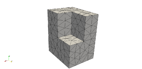
Figure 1: Domain with the initial mesh.

The goal of this test was to compute the eigenpair corresponding to the smallest positive eigenvalue. The exact eigenpairs of this problem are not known. Because of this, first, we have computed them with highly refined structured ‘uniform’ meshes, which allowed us to obtain by extrapolation a very accurate approximation of the corresponding eigenvalue. These ‘uniform’ meshes have been obtained by subdividing the domain in equal hexahedra, each of them subdivided into six tetrahedra. By so doing, we have obtained $\lambda=12.92$ as an approximate value of the smallest positive eigenvalue with four correct significant digits. This $\lambda$ was taken as the ‘exact’ eigenvalue.

Then, we have applied an adaptive scheme driven by the error indicators $\eta_{K}$. We have started the computations with the unstructured mesh consisting of $578$ elements shown in Figure 1 and have proceeded with the adaptive refinement process.

Figure 2 displays a log-log plot of the errors between the computed approximations of the smallest positive eigenvalue and the ‘exact’ one, versus the number of elements $N$ of the meshes. The figure shows the results obtained with ‘uniform’ meshes and with adaptively refined meshes.

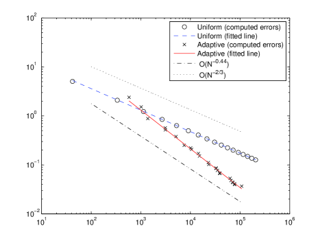
Figure 2: Error curves for the smallest positive eigenvalue of the Maxwell’s equations on the Fichera domain computed with ‘uniform’ and adaptively refined meshes: log-log plots of the respective errors versus the number of elements.

The very accurate agreement between the eigenvalues computed with ‘uniform’ meshes and the line obtained by a least square fitting of them is a clear indication of the reliability of the value taken as ‘exact’. The slope of the line is $-0.44$, which indicates that the errors of the eigenvalue computed with these ‘uniform’ meshes satisfy $\left|\lambda-\lambda_{h}\right|\approx CN^{-0.44}=Ch^{2t}$ with $t=0.66$.

It can be clearly seen from this figure that the eigenvalues computed with the adaptively refined meshes converge to the ‘exact’ one with a higher order of convergence than those computed with the ‘uniform’ meshes. Moreover, for similar number of elements $N$, the former are significantly smaller than the latter, which shows a neat advantage of using such and adaptive procedure. The figure also includes a dashed line with slope $-2/3$, which corresponds to the optimal order of convergence for the used lowest-order edge elements. The slope of the line obtained by a least squares fitting of the values computed with the adaptive scheme is a bit steeper: $-0.79$.

References

- Alonso et al. (2001) Alonso, A., Dello Russo, A., Padra, C. & Rodríguez, R. (2001) A posteriori error estimates and a local refinement strategy for a finite element method to solve structural-acoustic vibration problems. Adv. Comput. Math., 15, 25–59 (2002).
- Alonso et al. (2004) Alonso, A., Dello Russo, A., Padra, C. & Rodriguez, R. (2004) Accurate pressure post-process of a finite element method for elastoacoustics. Numer. Math., 98, 389–425.
- Amrouche et al. (1998) Amrouche, C., Bernardi, C., Dauge, M. & Girault, V. (1998) Vector potentials in three-dimensional non-smooth domains. Math. Methods Appl. Sci., 21, 823–864.
- Beck et al. (2000) Beck, R., Hiptmair, R., Hoppe, R. H. W. & Wohlmuth, B. (2000) Residual based a posteriori error estimators for eddy current computation. M2AN Math. Model. Numer. Anal., 34, 159–182.
- Boffi et al. (1999) Boffi, D., Fernandes, P., Gastaldi, L. & Perugia, I. (1999) Computational models of electromagnetic resonators: analysis of edge element approximation. SIAM J. Numer. Anal., 36, 1264–1290.
- Boffi (2000) Boffi, D. (2000) Fortin operator and discrete compactness for edge elements. Numer. Math., 87, 229–246.
- Boffi et al. (2012) Boffi, D., Gardini, F. & Gastaldi, L. (2012) Some remarks on eigenvalue approximation by finite elements. Frontiers in Numerical Analysis—Durham 2010. Lect. Notes Comput. Sci. Eng., vol. 85. Springer, Heidelberg, pp. 1–77.
- Boffi et al. (2013) Boffi, D., Brezzi, F. & Fortin, M. (2013) Mixed Finite Element Methods and Applications. Springer Series in Computational Mathematics, vol. 44. Springer, Heidelberg, pp. xiv+685.
- Boffi et al. (2015) Boffi, D., Gallistl, D., Gardini, F. & Gastaldi, L. (2015) Optimal convergence of adaptive fem for eigenvalue clusters in mixed form. Submitted.
- Braess & Schöberl (2008) Braess, D. & Schöberl, J. (2008) Equilibrated residual error estimator for edge elements. Math. Comp., 77, 651–672.
- Bürg (2011) Bürg, M. (2011) An hp-efficient residual-based a posteriori error estimator for Maxwell’s equations. Proc. Appl. Math. Mech., 11, 869 –870.
- Bürg (2012) Bürg, M. (2012) A residual-based a posteriori error estimator for the -finite element method for Maxwell’s equations. Appl. Numer. Math., 62, 922–940.
- Bürg (2013) Bürg, M. (2013) Convergence of an automatic -adaptive finite element strategy for Maxwell’s equations. Appl. Numer. Math., 72, 188–204.
- Caorsi et al. (2000) Caorsi, S., Fernandes, P. & Raffetto, M. (2000) On the convergence of Galerkin finite element approximations of electromagnetic eigenproblems. SIAM J. Numer. Anal., 38, 580–607.
- Chen et al. (2007) Chen, Z., Wang, L. & Zheng, W. (2007) An adaptive multilevel method for time-harmonic Maxwell equations with singularities. SIAM J. Sci. Comput., 29, 118–138.
- Clément (1975) Clément, P. (1975) Approximation by finite element functions using local regularization. Rev. Française Automat. Informat. Recherche Opérationnelle Sér. RAIRO Analyse Numérique, 9, 77–84.
- Cochez-Dhondt & Nicaise (2007) Cochez-Dhondt, S. & Nicaise, S. (2007) Robust a posteriori error estimation for the Maxwell equations. Comput. Methods Appl. Mech. Engrg., 196, 2583–2595.
- Creusé et al. (2012) Creusé, E., Nicaise, S., Tang, Z., Le Menach, Y., Nemitz, N. & Piriou, F. (2012) Residual-based a posteriori estimators for the magnetodynamic harmonic formulation of the Maxwell system. Math. Models Methods Appl. Sci., 22. 1150028, 30 pages.
- Creusé et al. (2013) Creusé, E., Nicaise, S., Tang, Z., Le Menach, Y., Nemitz, N. & Piriou, F. (2013) Residual-based a posteriori estimators for the magnetodynamic harmonic formulation of the Maxwell system. Int. J. Numer. Anal. Model., 10, 411–429.
- Durán et al. (1999) Durán, R. G., Gastaldi, L. & Padra, C. (1999) A posteriori error estimators for mixed approximations of eigenvalue problems. Math. Models Methods Appl. Sci., 9, 1165–1178.
- Durán et al. (2003) Durán, R. G., Padra, C. & Rodríguez, R. (2003) A posteriori error estimates for the finite element approximation of eigenvalue problems. Math. Models Methods Appl. Sci., 13, 1219–1229.
- Garau et al. (2009) Garau, E. M., Morin, P. & Zuppa, C. (2009) Convergence of adaptive finite element methods for eigenvalue problems. Math. Models Methods Appl. Sci., 19, 721–747.
- Gardini (2009) Gardini, F. (2009) Mixed approximation of eigenvalue problems: a superconvergence result. M2AN Math. Model. Numer. Anal., 43, 853–865.
- Giani & Graham (2009) Giani, S. & Graham, I. G. (2009) A convergent adaptive method for elliptic eigenvalue problems. SIAM J. Numer. Anal., 47, 1067–1091.
- Hannukainen (2008) Hannukainen, A. (2008) Functional type a posteriori error estimates for maxwell’s equations. Numerical Mathematics and Advanced Applications (K. Kunisch, G. Of & O. Steinbach eds). Springer Berlin Heidelberg, pp. 41–48.
- Harutyunyan et al. (2008) Harutyunyan, D., Izsák, F., van der Vegt, J. J. W. & Botchev, M. A. (2008) Adaptive finite element techniques for the Maxwell equations using implicit a posteriori error estimates. Comput. Methods Appl. Mech. Engrg., 197, 1620–1638.
- Jia et al. (2013) Jia, S., Chen, H. & Xie, H. (2013) A posteriori error estimator for eigenvalue problems by mixed finite element method. Sci. China Math., 56, 887–900.
- Larson (2000) Larson, M. G. (2000) A posteriori and a priori error analysis for finite element approximations of self-adjoint elliptic eigenvalue problems. SIAM J. Numer. Anal., 38, 608–625 (electronic).
- Lehoucq et al. (1998) Lehoucq, R. B., Sorensen, D. C. & Yang, C. (1998) ARPACK Users’ Guide. Philadelphia, PA: Society for Industrial and Applied Mathematics (SIAM), pp. xvi+142.
- Lin & Xie (2012) Lin, Q. & Xie, H. (2012) A superconvergence result for mixed finite element approximations of the eigenvalue problem. ESAIM Math. Model. Numer. Anal., 46, 797–812.
- Monk (1998) Monk, P. (1998) A posteriori error indicators for Maxwell’s equations. J. Comput. Appl. Math., 100, 173–190.
- Monk (2003) Monk, P. (2003) Finite Element Methods for Maxwell’s Equations. Numerical Mathematics and Scientific Computation. Oxford University Press, New York, pp. xiv+450.
- Monk & Demkowicz (2001) Monk, P. & Demkowicz, L. (2001) Discrete compactness and the approximation of Maxwell’s equations in . Math. Comp., 70, 507–523.
- Nicaise (2005) Nicaise, S. (2005) On Zienkiewicz-Zhu error estimators for Maxwell’s equations. C. R. Math. Acad. Sci. Paris, 340, 697–702.
- Nicaise & Creusé (2003) Nicaise, S. & Creusé, E. (2003) A posteriori error estimation for the heterogeneous Maxwell equations on isotropic and anisotropic meshes. Calcolo, 40, 249–271.
- Repin (2007) Repin, S. (2007) Functional a posteriori estimates for Maxwell’s equation. J. Math. Sci. (N. Y.), 142, 1821–1827.
- Schöberl (2008) Schöberl, J. (2008) A posteriori error estimates for Maxwell equations. Math. Comp., 77, 633–649.
- Si (2015) Si, H. (2015) TetGen, a Delaunay-based quality tetrahedral mesh generator. ACM Trans. Math. Software, 41, Art. 11, 36.
- Verfürth (1994) Verfürth, R. (1994) A posteriori error estimates for nonlinear problems. Finite element discretizations of elliptic equations. Math. Comp., 62, 445–475.