Universal transport and resonant current from chiral magnetic effect

For relativistic Weyl fermions in $3+1$ dimensions, an electric current proportional to the external magnetic field is predicted. This remarkable phenomenon is called Chiral Magnetic Effect (CME). Recent studies on “Weyl semimetals” in condensed matter physics renewed the interest on the subject as a realistic problem which can be investigated experimentally. Here we show that actual transports in Weyl semimetals supporting CME cannot be discussed without proper consideration of the law of electromagnetism. That is, the current and electromagnetic fields are not only related by the CME but also via electromagnetic induction and Ampère’s law. These intertwinings lead to observable transport properties governed by CME rather different from what one would expect naively from CME. First, even in the absence of an external magnetic field, CME leads to a material-independent, universal effective capacitance under certain conditions. Moreover, the induced current by a time-dependent external magnetic field can be resonantly enhanced reflecting a formation of electromagnetic standing waves. Our results imply that electromagnetism plays an essential role in electromagnetic properties of topological semimetals and its considerations is essential for the applications of CME to future electronics.

Interface between quantum field theory and condensed matter physics has been a source of many important developments. Weyl fermions and accompanying chiral anomaly is a particularly notable example. Their realization and consequences in condensed matter physics were discussed earlier as an offspring of the Nielsen-Ninomiya theorem in lattice field theory Nielsen and Ninomiya (1983), and then were revisited later in the context of quantum phase transitions Murakami (2007). More recently, a realization of Weyl fermions were predicted in pyrochlore iridates based on an ab initio calculation, and dubbed as Weyl semimetals Wan et al. (2011). This sparked a remarkable surge in the theoretical and experimental activities. Since then, Weyl semimetals have been reported to be experimentally confirmed in TaAs, NbP, and NbAs Lv et al. (2015a); Yang et al. (2015); Lv et al. (2015b); Belopolski et al. (2015); Xu et al. (2015), for example.

These developments bring up the hope that CME Fukushima et al. (2008) may be also observed experimentally Burkov (2015); Grushin (2012); Landsteiner (2014); Chernodub et al. (2014); Goswami and Tewari (2013); Goswami et al. (2015a); Chang and Yang (2015); Kharzeev (2014). Indeed, although it is still controversial Goswami et al. (2015b); Kikugawa et al. (2014), the giant negative quadratic magnetoresistance observed in Dirac semimetals Xiong et al. (2015); Huang et al. (2015) strongly suggests that the physics of relativistic fermions, in particular the chiral anomaly Son and Spivak (2013), is indeed taking place in these materials. However, at present there is no direct observation of CME in the original sense of an electric current driven by the external magnetic field. In the following, we explore possible observations of CME in terms of the induced current. In lattice models CME vanishes as a static effect in the thermal equilibrium Vazifeh and Franz (2013); Chen et al. (2013) but may exist in the non-equilibrium limit Goswami and Tewari (2013); Chang and Yang (2015). Thus we consider the CME at a finite frequency $\omega$, characterized by a finite chiral magnetic conductivity $\sigma_{ch}(\omega)$ so that

$$\bm{j}_{ch}(\omega)=\sigma_{ch}(\omega)\bm{B}(\omega).$$ (1)

However, there is an important issue to be addressed carefully for any discussion of possible observation of the CME: the electric and magnetic fields, and electric charge and current densities have to obey the laws of electrodynamics.

CME can be regarded as a Chern-Simons type extension of electromagnetism. As is known Wilczek (1987); Ooguri and Oshikawa (2012) in such cases the law of electromagnetism may lead to nontrivial responses. In this letter, by solving the Maxwell-Chern-Simons (MCS) equations we demonstrate that CME will qualitatively change transport properties of matter, in a rather unexpected way. As we will show, the physically observed conductance is not simply given by the chiral magnetic conductivity $\sigma_{ch}(\omega)$, even when it is governed by the CME. Our results imply that the electromagnetism is fundamental for actual transports in Weyl semimetals and that proposals for their applications to future electronics Kharzeev and Yee (2013) need careful considerations on this issue.

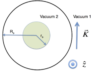
Figure 1: Schematic picture of our setup. A solenoid (radius $R_{s}$) is represented as a surface current between the two vacua. Inside them, a cylindrical sample (radius $r_{s}$) is placed.

We consider an infinitely long cylinder of the sample with nonzero chiral magnetic conductivity, placed inside an infinitely long solenoid (FIG.1). While any realistic system is of a finite length, we expect that our analysis essentially applies to such systems, as long as there is a non-vanishing uniform component along the cylinder axis in all the physical quantities including the current.

Fourier transforming in time, MCS equations inside the sample takes the following form:

$$\nabla\cdot\bm{B} =0$$ (2)

$$\nabla\cdot\bm{E} =\frac{\rho}{\epsilon}$$ (3)

$$\nabla\times\bm{E}-i\omega\bm{B} =0$$ (4)

$$\nabla\times\bm{B}+i\omega\epsilon\mu\bm{E} =\mu\sigma\bm{E}+\mu\sigma_{ch}\bm{B}$$ (5)

where $\rho$ is charge density, $\omega$ is frequency, $\sigma_{ch}(\omega)$ and $\sigma(\omega)$ respectively are chiral magnetic and ordinary longitudinal conductivity. For simplicity we do not consider the Hall effect. In the following, we assume $\mu\sigma\gg\omega/c^{2}$ and drop $i\omega/c^{2}\bm{E}$ inside the sample. To solve the MCS equations, we introduce the following dimensionless constant

$$\delta=\frac{\omega\sigma}{\mu\sigma_{ch}^{2}}$$ (6)

and consider a perturbative expansion of fields in terms of $\delta$. According an estimation for a lattice modelGoswami and Tewari (2013), when the energy difference between Weyl nodes is $\Delta$ [meV], $\sigma_{ch}$ is of the order of $10^{7}$ $\Delta$ $[\mathrm{A}/\mathrm{m^{2}T}]$. Since semimetals typically have $\sigma$ $\sim$ $10^{6}$ $[S/\mathrm{m}]$, $|\delta|$ is about $\delta\sim 10^{-2}\omega/\Delta^{2}$ for the frequency $\omega$ [Hz], if we assume $\mu\simeq\mu_{0}$. Therefore, if we assume $\Delta\sim 100$ [meV], our analysis works up to about $\omega\sim 100$ [kHz].

The geometry of our setup leads to the following conditions on fields, in terms of the cylindrical coordinates $(r,\phi,z)$:

$$\frac{\partial}{\partial\phi}\bm{E}=\frac{\partial}{\partial\phi}\bm{B}=\frac{\partial}{\partial z}\bm{E}=\frac{\partial}{\partial z}\bm{B}=B_{r}=E_{r}=0.$$ (7)

Under these conditions, the equations (2) and (3) are trivial. We shall solve the remaining equations (4) and (5) in the small-$\delta$ expansion. First we define a length scale $l_{\mathrm{CML}}=\pi/(\mu\sigma_{ch})$, which we call chiral magnetic length (CML). Here the factor $\pi$ is introduced for a later convenience. Scaling the radial coordinate $r$ as $\displaystyle x=\pi r/l_{\mathrm{CML}}$, at $\mathrm{O}(\delta^{0})$ we obtain

$$B_{z}(x) =aJ_{0}(x)$$ (8)

$$B_{\phi}(x) =aJ_{1}(x)$$ (9)

$$\bm{E}(x) =\frac{i\omega}{\mu\sigma_{ch}}\bm{B}(x),$$ (10)

where $J_{i}(x)$ represents $i$-th Bessel function and $a$ is an undetermined constant. Given the solutions (8) and (10), the parameter $\delta$ can be expressed as

$$\delta\simeq\left|\frac{\sigma E_{z}}{\sigma_{ch}B_{z}}\right|=\left|\frac{i\omega\sigma}{\mu\sigma_{ch}^{2}}\right|,$$ (11)

namely by the ratio of the ordinary current and the current due to CME. Therefore our analysis is physically a large CME expansion.

Electromagnetic fields in the “vacuum 2” region between the sample and the solenoid are derived in the Supplementary Material. In the lowest order of $\omega r_{s}/c$ and $\omega R_{s}/c$, they are given by:

$$B_{z}^{\mathrm{vac2}}(r) =-\frac{2i}{\pi c}\log\left[\frac{\omega}{c}r\right]e_{2}^{Y}+K$$ (12)

$$B_{\phi}^{\mathrm{vac2}}(r) =-\frac{2c}{\pi\omega}\frac{1}{r}b_{2}^{Y}$$ (13)

$$E_{z}^{\mathrm{vac2}}(r) =\frac{2ic}{\pi}\log\left[\frac{\omega}{c}r\right]b_{2}^{Y}.$$ (14)

$$E_{\phi}^{\mathrm{vac2}}(r) =-\frac{2c}{\pi\omega}\frac{1}{r}e_{2}^{Y}+\frac{i\omega}{2}Kr,$$ (15)

where $e_{2}^{Y}$ and $b_{2}^{Y}$ are undetermined constants. $K/\mu_{0}$ is the current flowing the solenoid in the angular direction per length of the cylinder. The three unknown coefficients, $a$, $e_{2}^{Y}$, and $b_{2}^{Y}$, are related by the two boundary conditions

$$(E_{\phi}^{\mathrm{cyl}}-E_{\phi}^{\mathrm{vac2}})|_{r=r_{s}}=(E_{z}^{\mathrm{cyl}}-E_{z}^{\mathrm{vac2}})|_{r=r_{s}}=0,$$ (16)

where $r_{s}$ is the radius of the cylindrical sample, and “cyl” denotes the fields inside the sample. Thus there is one remaining undetermined constant.

Below, we discuss transport properties of the cylinder based on the solutions we obtained. The total current $I_{z}^{\mbox{\scriptsize tot}}$ flowing along the cylindrical axis is simply given by

$$I_{z}^{\mbox{\scriptsize tot}}=-\frac{4c}{\mu_{0}\omega}b_{2}^{Y},$$ (17)

thanks to Ampère’s law and Eq. (13).

First, we consider a situation where a definite amount of current $I_{z}^{\mbox{\scriptsize tot}}$ is injected to the cylinder and the voltage drop along the cylindrical axis is measured. We can then define the complex electric conductance (admittance) $G$ by the ratio of $I_{z}^{\mbox{\scriptsize tot}}$ and $E_{z}L$, in which the residual undetermined constant $b_{2}^{Y}$ cancels. The admittance $G$ of a cylinder with length $L$ is then uniquely determined as $G=-i\omega C$, where

$$C =\frac{iI_{z}^{tot}}{\omega LE_{z}}\simeq\frac{2\pi}{\mu_{0}\omega^{2}L\,\log\left[\frac{c}{\omega r_{s}}\right]},$$ (18)

is real and positive in a realistic setting $\omega r_{s}\ll c$. That is, with the current leading the voltage by the phase $\pi/2$, the response in this order is purely capacitive with the effective capacitance (18). Qualitatively, this effective capacitive behavior may be understood as a consequence of the proportionality (10) between the magnetic and electric fields in the sample, and the local CME relation (1). The proportionality (10) implies that the admittance $G$, being the ratio between the voltage drop along the cylinder axis and the CME-induced current, does not depend on the solenoid current $K$. Thus, in terms of the admittance, the same capacitive transport governed by CME is observed even without applying any magnetic field externally ($K=0$)! We note that, while the setting and actual responses are different, there is a similarity between the capacitive transport and the screening of the electric field in “axionic” materials which is also related to the MCS Ooguri and Oshikawa (2012).

On the other hand, the quantitative estimate of the effective capacitance requires the analysis of the MCS equation with proper boundary conditions as described above. It is remarkable that the final result (18) does not contain any of the material parameters: $\epsilon$, $\mu$, $\sigma$, and $\sigma_{ch}$. Since our analysis is based on the macroscopic electromagnetism, all the details of the system are renormalized in those parameters. Therefore, the effective capacitance (18) is a material independent, universal quantity. It should be stressed that, although the formula (18) does not depend explicitly on the chiral magnetic conductivity $\sigma_{ch}$, it is a consequence of CME as it is obtained in the leading order in the large CME expansion. In any case, the result is quite different from what would be expected naively from CME without taking the law of electromagnetism into account.

Next, we evaluate the response of the total current $I_{z}^{\mbox{\scriptsize tot}}$ to the applied external magnetic field induced by the solenoid current $K$. Without taking the electromagnetism into account, it would be simply given by the cross section of the cylinder times the current density: $I_{z}^{tot}=\pi r_{s}^{2}\sigma_{ch}K$. However, we shall see that the result is rather different. In this case we have to specify the undetermined constant explicitly by imposing an additional condition. Here we assume that the “back-reaction” terms proportional to $e_{2}^{Y}$, which can only exist in the presence of the sample, are small compared to terms proportional to $K$. Then we have:

$$I_{z}^{tot} =\frac{\pi r_{s}J_{0}(\mu\sigma_{ch}r_{s})}{\mu_{0}J_{1}(\mu\sigma_{ch}r_{s})\log\left[\frac{c}{\omega r_{s}}\right]}K.$$ (19)

This current vanishes for $\omega\rightarrow 0$ due to the divergence of the denominator. As is known, CME in lattice models does not exist in thermal equilibrium. Here we obtained a stronger result: even if $\sigma_{ch}(\omega\rightarrow 0)$ is non-vanishing, the total current induced by a solenoid vanish (logarithmically) for $\omega\rightarrow 0$ if we take into account the law of electromagnetism.

In FIG. 2, we show $I_{z}^{tot}$ for the following parameters: $\mu\sigma_{ch}=1\mathrm{\,[mm^{-1}}],\,\omega=100\mathrm{\,[Hz]},\,B=1\mathrm{\,[Gauss]}$.

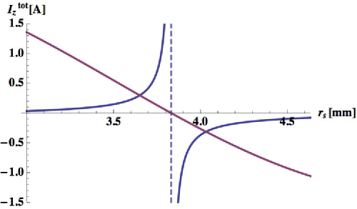
Figure 2: Blue line: Total current $I_{z}^{tot}$[A] for parameters $\mu\sigma_{ch}=1\mathrm{\,[mm^{-1}}],\omega=100\mathrm{\,[Hz]},B=1\mathrm{\,[Gauss]}$. Red: $J_{1}(\mu\sigma_{ch}r_{s})$ in an arbitrary unit. The current is resonantly enhanced for $r_{s}$ satisfying $J_{1}(\mu\sigma_{ch}r_{s})=0$ represented by a dashed line.

It is clear that the current is resonantly enhanced if $J_{1}(\mu\sigma_{ch}r_{s})=0$ is satisfied. Using the chiral magnetic length $l_{\mathrm{CML}}$, the condition is represented as:

$$\frac{r_{s}}{l_{\mathrm{CML}}}\simeq(\mathbb{Z}+\frac{1}{4})$$ (20)

since $J_{1}(y)\rightarrow\sqrt{2/\pi y}\cos(y-3\pi/4)$ for $y\rightarrow\infty$. $l_{\mathrm{CML}}$ is the characteristic length scale of electromagnetic fields inside the sample so the resonances correspond to formation of two-dimensional electromagnetic standing waves. As we noted, $\sigma_{ch}$ is about $10^{7}$ $\Delta$ where $\Delta$ is the energy difference between Weyl nodes in the unit of meV. $l_{\mathrm{CML}}=\pi/(\mu\sigma_{ch})$ is then given by $\sim 100\pi/\Delta$ [mm]. Therefore, when $\Delta=\mathrm{100}$[meV], the resonances will be achieved for $r_{s}\simeq\pi(\mathbb{Z}+1/4)$[mm].

Even away from the resonances, our result is still peculiar. If we assume $\mu\sigma_{ch}r_{s}\ll 1$, in the lowest order we have:

$$I_{z}^{tot}\simeq-\frac{2l_{\mathrm{CML}}}{\mu_{0}\log\left[\frac{\omega}{c}r_{s}\right]}K.$$ (21)

This means that in this parameter region, the induced current is monotonically “decreasing” as a function of $\sigma_{ch}$.

Appendix A Electromagnetic fields in the vacuum

To implement a solenoid in the framework of the Maxwell’s equations, we divide the vacuum region outside the material into two vacua (FIG. 1), inside and outside the solenoid. We then impose the following boundary conditions between them:

$$E_{z}^{\mathrm{vac}2}(r=R_{s})-E_{z}^{\mathrm{vac}1}(r=R_{s}) =0$$ (22)

$$E_{\phi}^{\mathrm{vac}2}(r=R_{s})-E_{\phi}^{\mathrm{vac}1}(r=R_{s}) =0$$ (23)

$$B_{z}^{\mathrm{vac}2}(r=R_{s})-B_{z}^{\mathrm{vac}1}(r=R_{s}) =K$$ (24)

$$B_{\phi}^{\mathrm{vac}2}(r=R_{s})-B_{\phi}^{\mathrm{vac}1}(r=R_{s}) =0$$ (25)

where “vac 1” and “vac 2” label the two vacua, $K$ models the current flowing the solenoid in the angular direction, and $R_{s}$ is the radius of the solenoid. Using (7), the fields are determined as a solution of the Maxwell’s equations in the vacuum:

$$E_{z}^{vac1,2}(r) =ic\left[\,b_{1,2}^{J}J_{0}\left(\frac{\omega}{c}r\right)+\,b_{1,2}^{Y}Y_{0}\left(\frac{\omega}{c}r\right)\right]$$ (26)

$$B_{\phi}^{vac1,2}(r) =b_{1,2}^{J}J_{1}\left(\frac{\omega}{c}r\right)+b_{1,2}^{Y}Y_{1}\left(\frac{\omega}{c}r\right)$$ (27)

$$B_{z}^{vac1,2}(r) =\frac{1}{ic}\left[e_{1,2}^{J}J_{0}\left(\frac{\omega}{c}r\right)+e_{1,2}^{Y}Y_{0}\left(\frac{\omega}{c}r\right)\right]$$ (28)

$$E_{\phi}^{vac1,2}(r) =e_{1,2}^{J}J_{1}\left(\frac{\omega}{c}r\right)+e_{1,2}^{Y}Y_{1}\left(\frac{\omega}{c}r\right).$$ (29)

Here $e_{1,2}^{J,Y}$ and $b_{1,2}^{J,Y}$ are undetermined constants and $J_{i},Y_{i}$ are Bessel functions of the first and second kind respectively. To determine the unknown coefficients, first we require causality in “vacuum 1” region. In other words, we require the non-existence of “incoming waves” from the infintiy. This is equivalent to force the fields to be regular in $\mathrm{Im}\,\omega>0$. Because both $J_{i}\left(\frac{\omega}{c}r\right)$ and $Y_{i}\left(\frac{\omega}{c}r\right)$ diverge for $\omega\rightarrow i\infty$, to meet the requirement, we have to take a linear combination of them to cancel out the divergence (notice that because we can take we can take $r\rightarrow\infty$ in this region, the unknown coefficients cannot regularize the divergence). Then it turns out that the Hankel function: $H_{i}\left(\frac{\omega}{c}r\right)=J_{i}\left(\frac{\omega}{c}r\right)+iY_{i}\left(\frac{\omega}{c}r\right)$ is the only combination regular in the upper half complex plane of $\omega$. Therefore, causality requires $e_{1}^{Y}=ie_{1}^{J}$ and $b_{1}^{Y}=ib_{1}^{J}$.

Then (22)$\sim$(25) give the following results with only two unknown coefficients $e_{2}^{Y}$ and $b_{2}^{Y}$:

$$E_{z}^{\mathrm{vac2}} =c\,b_{2}^{Y}H_{0}^{r}$$ (30)

$$B_{\phi}^{\mathrm{vac2}} =-i\,b_{2}^{Y}H_{1}^{r}$$ (31)

$$B_{z}^{\mathrm{vac2}} =-\frac{1}{c}e_{2}^{Y}H_{0}^{r}-\frac{\pi}{2ic}\omega R_{s}H_{1}^{R_{s}}KJ_{0}^{r}$$

$$E_{\phi}^{\mathrm{vac2}} =-ie_{2}^{Y}H_{1}^{r}-\frac{\pi}{2}\omega R_{s}H_{1}^{R_{s}}KJ_{1}^{r}$$

where we have used abbreviated notations like $H_{i}(\omega R_{s}/c)\equiv H_{i}^{R_{s}}$ and $J_{i}(\omega R_{c}/c)\equiv J_{i}^{R_{s}}$.

References

- Nielsen and Ninomiya (1983) H.B. Nielsen and Masao Ninomiya, “The Adler-Bell-Jackiw anomaly and Weyl fermions in a crystal,” Physics Letters B 130, 389 – 396 (1983).
- Murakami (2007) Shuichi Murakami, “Phase transition between the quantum spin Hall and insulator phases in 3D: emergence of a topological gapless phase,” New Journal of Physics 9, 356 (2007).
- Wan et al. (2011) Xiangang Wan, Ari M. Turner, Ashvin Vishwanath, and Sergey Y. Savrasov, “Topological semimetal and Fermi-arc surface states in the electronic structure of pyrochlore iridates,” Phys. Rev. B 83, 205101 (2011).
- Lv et al. (2015a) B. Q. Lv, H. M. Weng, B. B. Fu, X. P. Wang, H. Miao, J. Ma, P. Richard, X. C. Huang, L. X. Zhao, G. F. Chen, Z. Fang, X. Dai, T. Qian, and H. Ding, “Experimental Discovery of Weyl Semimetal TaAs,” Phys. Rev. X 5, 031013 (2015a).
- Yang et al. (2015) L. X. Yang, Z. K. Liu, Y. Sun, H. Peng, H. F. Yang, T. Zhang, B. Zhou, Y. Zhang, Y. F. Guo, M. Rahn, D. Prabhakaran, Z. Hussain, S. K. Mo, C. Felser, B. Yan, and Y. L. Chen, “Weyl semimetal phase in the non-centrosymmetric compound TaAs,” Nat Phys 11, 728–732 (2015).
- Lv et al. (2015b) B. Q. Lv, N. Xu, H. M. Weng, J. Z. Ma, P. Richard, X. C. Huang, L. X. Zhao, G. F. Chen, C. E. Matt, F. Bisti, V. N. Strocov, J. Mesot, Z. Fang, X. Dai, T. Qian, M. Shi, and H. Ding, “Observation of Weyl nodes in TaAs,” Nat Phys 11, 724–727 (2015b).
- Belopolski et al. (2015) I. Belopolski, S.-Y. Xu, D. Sanchez, G. Chang, C. Guo, M. Neupane, H. Zheng, C.-C. Lee, S.-M. Huang, G. Bian, N. Alidoust, T.-R. Chang, B. Wang, X. Zhang, A. Bansil, H.-T. Jeng, H. Lin, S. Jia, and M. Zahid Hasan, “Observation of surface states derived from topological Fermi arcs in the Weyl semimetal NbP,” ArXiv e-prints (2015), arXiv:1509.07465 [cond-mat.mes-hall] .
- Xu et al. (2015) Su-Yang Xu, Nasser Alidoust, Ilya Belopolski, Zhujun Yuan, Guang Bian, Tay-Rong Chang, Hao Zheng, Vladimir N. Strocov, Daniel S. Sanchez, Guoqing Chang, Chenglong Zhang, Daixiang Mou, Yun Wu, Lunan Huang, Chi-Cheng Lee, Shin-Ming Huang, BaoKai Wang, Arun Bansil, Horng-Tay Jeng, Titus Neupert, Adam Kaminski, Hsin Lin, Shuang Jia, and M. Zahid Hasan, “Discovery of a Weyl fermion state with Fermi arcs in niobium arsenide,” Nat Phys 11, 748–754 (2015).
- Fukushima et al. (2008) Kenji Fukushima, Dmitri E. Kharzeev, and Harmen J. Warringa, “Chiral magnetic effect,” Phys. Rev. D 78, 074033 (2008).
- Burkov (2015) A A Burkov, “Chiral anomaly and transport in Weyl metals,” Journal of Physics: Condensed Matter 27, 113201 (2015).
- Grushin (2012) Adolfo G. Grushin, “Consequences of a condensed matter realization of Lorentz-violating QED in Weyl semi-metals,” Phys. Rev. D 86, 045001 (2012).
- Landsteiner (2014) Karl Landsteiner, “Anomalous transport of Weyl fermions in Weyl semimetals,” Phys. Rev. B 89, 075124 (2014).
- Chernodub et al. (2014) Maxim N. Chernodub, Alberto Cortijo, Adolfo G. Grushin, Karl Landsteiner, and María A. H. Vozmediano, “Condensed matter realization of the axial magnetic effect,” Phys. Rev. B 89, 081407 (2014).
- Goswami and Tewari (2013) Pallab Goswami and Sumanta Tewari, “Chiral magnetic effect of Weyl fermions and its applications to cubic noncentrosymmetric metals,” ArXiv e-prints (2013), arXiv:1311.1506 [cond-mat.mes-hall] .
- Goswami et al. (2015a) Pallab Goswami, Girish Sharma, and Sumanta Tewari, “Optical activity as a test for dynamic chiral magnetic effect of Weyl semimetals,” Phys. Rev. B 92, 161110 (2015a).
- Chang and Yang (2015) Ming-Che Chang and Min-Fong Yang, “Chiral magnetic effect in a two-band lattice model of Weyl semimetal,” Phys. Rev. B 91, 115203 (2015).
- Kharzeev (2014) Dmitri E. Kharzeev, “The Chiral Magnetic Effect and anomaly-induced transport,” Progress in Particle and Nuclear Physics 75, 133 – 151 (2014).
- Goswami et al. (2015b) Pallab Goswami, J. H. Pixley, and S. Das Sarma, “Axial anomaly and longitudinal magnetoresistance of a generic three-dimensional metal,” Phys. Rev. B 92, 075205 (2015b).
- Kikugawa et al. (2014) N. Kikugawa, P. Goswami, A. Kiswandhi, E. S. Choi, D. Graf, R. E. Baumbach, J. S. Brooks, K. Sugii, Y. Iida, M. Nishio, S. Uji, T. Terashima, P. M. C. Rourke, N. E. Hussey, H. Takatsu, S. Yonezawa, Y. Maeno, and L. Balicas, “Inter-planar coupling dependent magnetoresistivity in high purity layered metals,” ArXiv e-prints (2014), arXiv:1412.5168 [cond-mat.mes-hall] .
- Xiong et al. (2015) Jun Xiong, Satya K. Kushwaha, Tian Liang, Jason W. Krizan, Max Hirschberger, Wudi Wang, R. J. Cava, and N. P. Ong, “Evidence for the chiral anomaly in the Dirac semimetal Na3Bi,” Science 350, 413–416 (2015).
- Huang et al. (2015) Xiaochun Huang, Lingxiao Zhao, Yujia Long, Peipei Wang, Dong Chen, Zhanhai Yang, Hui Liang, Mianqi Xue, Hongming Weng, Zhong Fang, Xi Dai, and Genfu Chen, “Observation of the Chiral-Anomaly-Induced Negative Magnetoresistance in 3D Weyl Semimetal TaAs,” Phys. Rev. X 5, 031023 (2015).
- Son and Spivak (2013) D. T. Son and B. Z. Spivak, “Chiral anomaly and classical negative magnetoresistance of Weyl metals,” Phys. Rev. B 88, 104412 (2013).
- Vazifeh and Franz (2013) M. M. Vazifeh and M. Franz, “Electromagnetic Response of Weyl Semimetals,” Phys. Rev. Lett. 111, 027201 (2013).
- Chen et al. (2013) Y. Chen, Si Wu, and A. A. Burkov, “Axion response in Weyl semimetals,” Phys. Rev. B 88, 125105 (2013).
- Wilczek (1987) Frank Wilczek, “Two applications of axion electrodynamics,” Phys. Rev. Lett. 58, 1799–1802 (1987).
- Ooguri and Oshikawa (2012) Hirosi Ooguri and Masaki Oshikawa, “Instability in Magnetic Materials with a Dynamical Axion Field,” Phys. Rev. Lett. 108, 161803 (2012).
- Kharzeev and Yee (2013) Dmitri E. Kharzeev and Ho-Ung Yee, “Anomaly induced chiral magnetic current in a Weyl semimetal: Chiral electronics,” Phys. Rev. B 88, 115119 (2013).