Querying Evolving Graphs with Portal

Abstract

Graphs are used to represent a plethora of phenomena, from the Web and social networks, to biological pathways, to semantic knowledge bases. Arguably the most interesting and important questions one can ask about graphs have to do with their evolution. Which Web pages are showing an increasing popularity trend? How does influence propagate in social networks? How does knowledge evolve?

This paper proposes a logical model of an evolving graph called a TGraph, which captures evolution of graph topology and of its vertex and edge attributes. We present a compositional temporal graph algebra TGA, and show a reduction of TGA to temporal relational algebra with graph-specific primitives. We formally study the properties of TGA, and also show that it is sufficient to concisely express a wide range of common use cases. We describe an implementation of our model and algebra in Portal, built on top of Apache Spark / GraphX. We conduct extensive experiments on real datasets, and show that Portal scales.

1 Introduction

The importance of networks in scientific and commercial domains cannot be overstated. Considerable research and engineering effort is being devoted to developing effective and efficient graph representations and analytics. Efficient graph abstractions and analytics for static graphs are available to researchers and practitioners in scope of open source platforms such as Apache Giraph, Apache Spark / GraphX [18] and GraphLab / PowerGraph [17].

Arguably the most interesting and important questions one can ask about networks have to do with their evolution, rather than with their static state. Analysis of evolving graphs has been receiving increasing attention [2, 9, 22, 29, 30, 32]. Yet, despite much recent activity, and despite increased variety and availability of evolving graph data, systematic support for scalable querying and analysis of evolving graphs still lacks. This support is urgently needed, due first and foremost to the scalability and efficiency challenges inherent in evolving graph analysis, but also to considerations of usability and ease of dissemination. The goal of our work is to fill this gap. In this paper, we present an algebraic query language called TGraph algebra, or TGA, and its scalable implementation in Portal, an open-source distributed framework on top of Apache Spark.

Our goal in developing TGA is to give users an ability to concisely express a wide range of common analysis tasks over evolving graphs, while at the same time preserving inter-operability with temporal relational algebra (TRA). Implementing (non-temporal) graph querying and analytics in an RDBMS has been receiving renewed attention [1, 33, 36], and our work is in-line with this trend. Our data model is based on the temporal relational model, and our algebra corresponds to temporal relational algebra, but is designed specifically for evolving graphs.

We represent graph evolution, including changes in topology and in attribute values of vertices and edges, using the TGraph abstraction — a collection of temporal SQL relations with appropriate integrity constraints. An example of a TGraph is given in Figure 1, where we show evolution of a co-authorship network.

TGA can be viewed as TRA for graphs, and so does not support general recursion or transitive closure computation. (Although, as we will see in Section 3.7, Pregel-style graph analytics such as PageRank are supported as an extension.) For this reason, we also do not support regular path queries (RPQ) or the more general path query classes (CRPQ and ECRPQ). Extending our formalism with recursion and path queries is non-trivial, and we leave this to future work.

Rather than focusing on path computation and graph traversal, we stress the tasks that perform whole-graph analysis over time. Several such tasks are described next. Additional examples can be found in SocialScope [3] — a closed non-temporal algebra for multigraphs that is motivated by information discovery in social content sites. It is not difficult to show that the graph (rather than multigraph) versions of all SocialScope operations can be expressed, and augmented with the temporal dimension, in TGA.

1.1 Use cases and algebra by example

An interaction network is one typical kind of an evolving graph. It represents people as vertices, and interactions between them such as messages, conversations and endorsements, as edges. Information describing people and their interactions is represented by vertex and edge attributes. One easily accessible interaction network is the wiki-talk dataset (http://dx.doi.org/10.5281/zenodo.49561), containing messaging events among Wikipedia contributors over a 13-year period. Information available about the users includes their username, group membership, and the number of Wikipedia edits they made. Messaging events occur when users post on each other’s talk pages.

We now present common analysis tasks that motivate the operators of our algebra, TGA.

Vertex influence over time. In an interaction graph, vertex centrality is a measure of how important or influential people are. Over a dozen different centrality measures exist, providing indicators of how much information “flows” through the vertex or how the vertex contributes to the overall cohesiveness of the network. Vertex importance fluctuates over time. To see whether the wiki-talk graph has high-importance vertices, and how stable vertex importance is over time during a particular period of interest, we can look at a subset of the graph that corresponds to the period of interest, compute an importance measure, such as in-degree, for each vertex and for each point in time, and finally calculate the coefficient of variation per vertex.

Question: What are the high-influence nodes over the past 5 years, and is their influence persistent over time?

1. Select a subset of the data representing the 5 years of interest, using a common temporal operator slice($\tau$):
   $\mathsf{T}_{1}=\tau_{[2010,2015)}(wikitalk)$

2. Compute in-degree (prominence) of each vertex during each time point. This is an example of the aggregation operation, a common operation on non-temporal graphs, as defined by the taxonomy of Wood [35]. Aggregation computes a value for each vertex based on its neighbors. SocialScope [3] is one of the languages that proposes an aggregation operation and demonstrates its many uses. We introduce a temporal version of aggregation (listed here with default arguments omitted for readability):
   $\mathsf{T}_{2}=\textsf{agg}^{T}(\mathsf{dir=right},\mathsf{f_{m}=1},\mathsf{f_{a}=count},\mathsf{pname=deg},\mathsf{T}_{1})$

3. Aggregate degree information per vertex across the timespan of $\mathsf{T}_{2}$, collecting values into a map. This is an example of aggregation based on temporal window, which we implement with the temporal node creation operator:
   $\mathsf{T}_{3}=\textsf{node}^{T}_{w}(\mathsf{w=lifetime},\mathsf{f_{v}=\{map(deg)\}},\mathsf{T}_{2})$

4. Transform the attributes of each vertex to compute the coefficient of variation from the map of degree values, using the temporal vertex-map operator:
   $\mathsf{T}_{4}=\textsf{map}^{T}_{v}(\mathsf{f_{v}=stdev(deg)/mean(deg)*100},\mathsf{T}_{3})$

Graph centrality over time. Graph centrality is a popular measure that is used to evaluate how connected or centralized the community is. This measure can be computed by aggregating in-degree values of graph vertices and may change as communication patterns evolve, or as high influencers appear or disappear. In sparse interaction graphs there is an additional question of temporal resolution to consider: if two people communicated on May 16, 2010, how long do we consider them to be connected? We now show how graph centrality can be computed over time, with control for temporal resolution.

Question: How has graph centrality changed over time?

1. Compute a temporally aggregated view of the graph into 2-months windows. Each window will include vertices and edges that communicate frequently: a vertex and an edge are each present during a 2-month window if they exist in every snapshot during that period. We use the window-based node creation operation.
   $\mathsf{T}_{1}=\textsf{node}^{T}_{w}(\mathsf{w=2~{}mon},\mathsf{q_{v}=always},\mathsf{q_{e}=always},wikitalk)$

2. Compute in-degree of each vertex:
   $\mathsf{T}_{2}=\textsf{agg}^{T}(\mathsf{dir=right},\mathsf{f_{m}=1},\mathsf{f_{a}=count},\mathsf{pname=deg},\mathsf{T}_{1})$

3. Create a new graph, in which all vertices that are present at a given time point (snapshot) are grouped into a single vertex. Accumulate maximum, sum and count of the values of $deg$ as properties at that vertex. We implement this with the attribute-based node creation operation. Creating a single vertex to represent the whole graph is one use of node creation. We will show that node creation is useful for other types of analysis. $\mathsf{T}_{3}=$
   $\textsf{node}^{T}_{a}(\mathsf{g=1,f_{v}=\{max(deg),~{}sum(deg),~{}count(deg)\}},\mathsf{T}_{2})$

4. Compute degree centrality at each time point.
   $\mathsf{T}_{4}=\textsf{map}^{T}_{v}(\mathsf{f_{v}=(max*cnt-sum)/(cnt^{2}-3*cnt+2)},\mathsf{T}_{3})$

Communities over time. Interaction networks are sparse because edges are so short-lived. As part of exploratory analysis, we can consider the network at different temporal resolutions, run a community detection algorithm, e.g., compute the connected components of the network, and then consider the number of and size of connected components.

Question: In a sparse communication network, on what time scale can we detect communities?

1. Aggregate the graph into 6-month windows.
   $\mathsf{T}_{1}=\textsf{node}^{T}_{w}(\mathsf{w=6~{}mon},\mathsf{q_{v}=always},\mathsf{q_{e}=always},wikitalk)$

2. Compute connected components at each time point. This is an example of a Pregel-style analytic invocation over an evolving graph. $\mathsf{T}_{2}=\textsf{pregel}^{T}_{cc}(\mathsf{pname=comp},\mathsf{T}_{1})$

3. Generate a new graph, in which a vertex corresponds to a connected component, and compute the size of the connected component. $\mathsf{T}_{3}=\textsf{node}^{T}_{a}(\mathsf{g=comp,f_{v}=count(1)},\mathsf{T}_{2})$

4. Filter out vertices that represent communities too small to be useful (e.g., of 1-2 people). This is an example of vertex subgraph. $\mathsf{T}_{4}=\textsf{sub}^{T}_{v}(\mathsf{v.a.count>2},\mathsf{T}_{3})$

In Section 3 we formally define the operators of our graph algebra. In Section 6 we return to these three use cases.

1.2 Contributions and roadmap

We propose a representation of an evolving graph, called a TGraph, which captures the evolution of both graph topology and vertex and edge attributes (Section 2), and develop a compositional TGraph algebra, TGA (Section 3). We show a reduction from TGA to temporal relational algebra TRA, using a combination of standard operators and TGraph-specific primitives, and present formal properties of TGA (Section 4). We present an implementation in scope of the Portal system, built on Apache Spark / GraphX [18]. Portal supports several access methods that correspond to different trade-offs in temporal and structural locality (Section 5). We conduct an extensive experimental evaluation with real datasets, demonstrating that Portal scales (Section 6). We also illustrate the usability throughout the paper, with a variety of real-life analysis tasks that can be concisely expressed in TGA.

2 Data Model

Following the SQL:2011 standard [25], a period (or interval) $\mathbf{p}=[s,e)$ represents a discrete set of time instances, starting from and including the start time $s$, continuing to but excluding the end time $e$. Time instances contained within the period have limited precision, and the time domain has total order.

Figure 1: TGraph T1.

We now describe the logical representation of an evolving graph, called a TGraph. A TGraph represents a single graph, and models evolution of its topology and of vertex and edge attributes. Figure 1 gives an example of a TGraph that shows evolution of a co-authorship network.

A TGraph is represented with four temporal SQL relations [5], and uses point semantics [34], associating a fact (existence of a vertex or edge, and an assignment of a value to a vertex or edge attribute) with a time point. We use periods to compactly represent their constituent time points. This is a common representation technique, which does not add expressive power to the data model [10].

A snapshot of a temporal relation $R$, denoted $\tau^{s}_{c}(R)$ (“s” stands for “snapshot”), is the state of $R$ at time point $c$.

We use the property graph model [31] to represent vertex and edge attributes: each vertex and edge during period $\mathbf{p}$ is associated with a (possibly empty) set of properties, and each property is represented by a key-value pair. Property values are not restricted to be of atomic types, and may, e.g., be sets, maps or tuples.

We now give a formal definition of a TGraph.

Definition 2.1 (TGraph)

A TGraph is a pair $\mathsf{T}=(\textsf{TV},\textsf{TE})$. TV is a valid-time temporal SQL relation with schema $\textsf{TV}(\underline{v},\underline{\mathbf{p}})$ that associates a vertex with the time period during which it is present. TE is a valid-time temporal SQL relation with schema $\textsf{TE}(\underline{v_{1}},\underline{v_{2}},\underline{\mathbf{p}})$, connecting pairs of vertices from TV. $\mathsf{T}$ optionally includes vertex and edge attribute relations $\mathsf{TA^{V}}(\underline{v},\underline{\mathbf{p}},a)$ and $\mathsf{TA^{E}}(\underline{v_{1}},\underline{v_{2}},\underline{\mathbf{p}},a)$. Relations of $\mathsf{T}$ must meet the following requirements:

R1: Unique vertices/ edges

In every snapshot $\tau^{s}_{c}(\mathsf{TA^{V}})$ and $\tau^{s}_{c}(\mathsf{TA^{E}})$, where $c$ is a time point, a vertex/edge exists at most once.

R2: Unique attribute values

In every snapshot $\tau^{s}_{c}(\mathsf{TA^{V}})$ and $\tau^{s}_{c}(\mathsf{TA^{E}})$, a vertex/edge is associated with at most one attribute (which is itself a set of key-value pairs representing properties).

R3: Referential integrity

In every snapshot $\tau^{s}_{c}(\mathsf{T})$, foreign key constraints hold from $\tau^{s}_{c}(\textsf{TE})$ (on both $v_{1}$ and $v_{2}$) and $\tau^{s}_{c}(\mathsf{TA^{V}})$ to $\tau^{s}_{c}(\textsf{TV})$, and from $\tau^{s}_{c}(\mathsf{TA^{E}})$ to $\tau^{s}_{c}(\textsf{TE})$.

R4: Coalesced

Value-equivalent tuples in all relations of $\mathsf{T}$ with consecutive or overlapping time periods are merged.

Requirements R1, R2, R3 guarantee soundness of the TGraph data structure, ensuring that every snapshot of a TGraph is a valid graph. Requirement R4 avoids semantic ambiguity and ensures correctness of algebraic operations in point-stamped temporal models such as ours [21].

Graphs may be directed or undirected. For undirected graphs we choose a canonical representation of an edge, with $v_{1}\leq v_{2}$ (self-loops are allowed). Because we use the source and destination vertex id pair as the identifier for the edges, at most two edges can exist between any two vertices (one in each direction) at any time point. That is, we do not support multigraphs.

In the TGraph representation of Definition 2.1, vertex and edges attributes are stored as collections of properties. That said, Definition 2.1 presents a logical data structure that admits different physical representations, including, e.g., a columnar representation (each property in a separate relation, supporting different change rates), by a hash-based representation of [33], or in some other way. We leave an experimental comparison of different physical representations of vertex and edge attributes to future work.

Our choice to use attribute relations is in contrast to representing vertex and edge attributes as part of TV and TE. The main reason is to streamline the enforcement of referential integrity constraints of Definition 2.1. Consider again the example in Figure 1. If vertex attributes were stored as part of TV, then there would be two tuples for $v_{2}$ in this relation whose validity periods overlap with that of edge $e(v_{1},v_{2})$ — one for each $[2/15,5/15)$ and $[5/15,7/15)$. This would in turn require that $e(v_{1},v_{2})$ be mapped to two tuples in TV as part of referential integrity checking on $v_{2}$. Matching a tuple with a set of tuples in the referenced table, while supported by the SQL:2011 standard, is potentially inefficient, and we avoid it in our representation. Another reason for storing $\mathsf{TA^{V}}$ and $\mathsf{TA^{E}}$ separately is that in many cases we are interested in applying operations (e.g., analytics) only to graph topology, and in that case TV and TE are sufficient.

3 Algebra

TGraph algebra, or TGA for short, is compositional: operators take a TGraph or a pair of TGraphs as input, and output a TGraph. We specify the semantics of TGA by showing a translation of each operator into a sequence of temporal relational algebra (TRA) expressions (with nesting, to accommodate non-1NF vertex/edge attributes). Using this translation one can implement TGA in a temporal DBMS, guaranteeing snapshot reducibility and extended snapshot reducibility [6] — two properties that are appropriate for a point-based temporal data model.

TRA algebra extends relational algebra by specifying how operators are applied to temporal relations such that snapshot reducibility property is guaranteed. Additionally, explicit references to time are supported in operator predicates (extended snapshot reducibility), but the time stamps are not manipulated by the user queries directly.

In Section 3.1 we present the primitives that are needed to enforce soundness of TGA. Then, in Sections 3.2 through 3.6, we present TGA operators. Section 3.7 presents an extension of TGA to support Pregel-style analytics.

3.1 Primitives and Soundness

TGA operators are translated into expressions in temporal relational algebra (TRA). Since TRA is applied to individual relations of $\mathsf{T}$, we must ensure that the combined state of these relations in the result corresponds to a valid TGraph, i.e., that the translation is sound. Recall from Definition 2.1 that a valid TGraph must satisfy four requirements: R1: Unique vertices and edges, R2: Unique attribute values, R3: Referential integrity, and R4: Coalesced. We now describe four primitives that will ensure soundness of TGA.

Coalesce. To enforce requirements R1 and R4, we introduce the coalesce primitive $\mathcal{C}(R)$, which merges adjacent or overlapping time periods for value-equivalent tuples. This operation is similar to duplicate elimination in conventional databases, and has been extensively studied in the literature [5, 38]. $\mathcal{C}(R)$ is applied to individual relations of $\mathsf{T}$, or to intermediate results, following the application of operations that uncoalesce. The coalesce primitive can be implemented in relational algebra [5]. If a DBMS supports automatic coalescing, this primitive is not necessary.

Resolve. To enforce R2 we introduce the resolve primitive $\mathcal{R}(f_{1}(k_{1}),\ldots,f_{n}(k_{n}),R)$, which is invoked by operations that produce attribute relations with duplicates. Resolve computes a temporal group-by of the attribute relation $R$ by key (e.g., by $v$ if $R$ represents vertex attributes). It then computes a bag-union of the properties occurring in each group, groups together key-value pairs that correspond to the same property name $k_{i}$, and aggregates values within each group using the specified aggregation function $f_{i}$. If no aggregation function is specified for a particular property name, set is used as the default. For example, if $R$ contains tuples $(v_{1},[2/15,4/15),\{name=Ann,sal=100\})$ and $(v_{1},[2/15,3/15),\{name=Ann,sal=200\})$, the result of $\mathcal{R}(AVG(sal),R)$ will contain $(v_{1},[2/15,3/15),\{name=Ann,sal=150\})$ and $(v_{1},[3/15,4/15),\{name=Ann,sal=100\})$. The resolve primitive can be implemented with temporal relational aggregation $\gamma^{T}$ over unnested relations.

Constrain. To enforce R3 we introduce the constrain primitive $\mathcal{K}(r,s)$, which enforces referential integrity on relation $\mathbf{r}$ with respect to relation $\mathbf{s}$. For example, this primitive is used to remove edges from TE for which one or both vertices are absent from TV, or restrict the validity period of an edge to be within the validity periods of its vertices.

Split. The final primitive $\mathcal{S}(s,w,R)$ uncoalesces relation $R$ in a particular way. For each tuple $t\in R$ with time period $p$, it emits a set of tuples, with the same values for non-temporal attributes as in $t$, but with time periods split into windows of width $w$ with respect to start time $s$. For example, $\mathcal{S}(2/15,3~{}\textsf{months},\textsf{TE})$ for T1 in Figure 1 produces an uncoalesced relation with 2 tuples for $(v_{1},v_{2})$, with periods $[2/15,5/15)$ and $[5/15,6/15)$, and 2 tuples for $(v_{2},v_{3})$, with validity periods $[7/15,8/15)$ and $[8/15,10/15)$. This primitive will be necessary to express the temporal variant of node creation (Section 3.5). It will be used at an intermediate step in the computation, all final results will be coalesced as needed, enforcing R4.

3.2 Unary operators

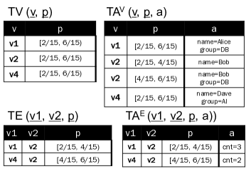
Figure 2: T2.

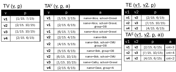
Figure 3: $T1\cup^{T}T2.$

Slice. The slice operator, denoted $\tau_{\mathbf{c}}(\mathsf{T})$, where $\mathbf{c}$ is a time interval, cuts a temporal slice from $\mathsf{T}$. The resulting TGraph will contain vertices and edges whose period $\mathbf{p}$ has a non-empty intersection with $\mathbf{c}$. We translate this TGA operator to TRA statements over each constituent relation of $\mathsf{T}$: $\tau_{\mathbf{c}}(\textsf{TV})$ and similarly for TE, $\mathsf{TA^{V}}$ and $\mathsf{TA^{E}}$.

Subgraph. Temporal subgraph matching is a generalization of subgraph matching for non-temporal graphs [35]. This query comes in two variants.

Temporal vertex-subgraph $\textsf{sub}^{T}_{v}(q^{t}_{v},\mathsf{T})$ computes an induced subgraph of $\mathsf{T}$ $\mathsf{T}^{\prime}(\textsf{TV}^{\prime},\textsf{TE}^{\prime},\mathsf{TA^{V}}^{\prime},\mathsf{TA^{E}}^{\prime})$, with vertices defined by the temporal conjunctive query (TCQ) $q^{t}_{v}$. Note that this is a subgraph query, and so $\textsf{TV}^{\prime}\subseteq^{T}\textsf{TV}$.

Temporal edge-subgraph $\textsf{sub}^{T}_{e}(q^{t}_{e},\mathsf{T})$ computes a subgraph of $\mathsf{T}$ $\mathsf{T}^{\prime}(\textsf{TV}^{\prime},\textsf{TE}^{\prime},\mathsf{TA^{V}}^{\prime},\mathsf{TA^{E}}^{\prime})$ in which edges are defined by TCQ $q^{t}_{e}$. Since this is a subgraph query, $\textsf{TE}^{\prime}\subseteq^{T}\textsf{TE}$.

Queries $q^{t}_{v}$ and $q^{t}_{e}$ may use any of the constituent relations of $\mathsf{T}$, and may explicitly reference temporal information, and so require all input relations to be coalesced [4].

Following the computation of $\textsf{TV}^{\prime}=q^{t}_{v}(\textsf{TV})$, $\textsf{sub}^{T}_{v}(q^{t}_{v},\mathsf{T})$ must invoke $\mathcal{C}(\textsf{TV}^{\prime})$ to enforce R1 and R4; and $\mathcal{K}(\textsf{TE}^{\prime},\textsf{TV}^{\prime})$, $\mathcal{K}(\mathsf{TA^{V}}^{\prime},\textsf{TV}^{\prime})$, $\mathcal{K}(\mathsf{TA^{E}}^{\prime},\textsf{TE}^{\prime})$ to enforce R3. Following the computation $\textsf{TE}^{\prime}=q^{t}_{e}(\textsf{TE})$, $\textsf{sub}^{T}_{e}(q^{t}_{e},\mathsf{T})$ must invoke $\mathcal{C}(\textsf{TE}^{\prime})$ to enforce R1 and R4; and $\mathcal{K}(\mathsf{TA^{E}}^{\prime},\textsf{TE}^{\prime})$ to enforce R3.

Map. Temporal vertex-map and edge-map apply user-defined map functions $f_{v}$ and $f_{e}$ to vertex or edge attributes. Temporal vertex-map $\textsf{map}^{T}_{v}(f_{v},\mathsf{T})$ outputs $\mathsf{T}^{\prime}$ in which $\textsf{TV}^{\prime}=\textsf{TV}$, $\textsf{TE}^{\prime}=\textsf{TE}$, $\mathsf{TA^{E}}^{\prime}=\mathsf{TA^{E}}$, and $\mathsf{TA^{V}}^{\prime}=\pi^{T}_{v,f_{v}(a)}\mathsf{TA^{V}}$. Temporal edge-map $\textsf{map}^{T}_{e}(f_{e},\mathsf{T})$ is defined analogously.

While $f_{v}$ and $f_{e}$ are arbitrary user-specified functions, there are some common cases. Map may specify the set of properties to project out or retain, it may aggregate (e.g., COUNT) or deduplicate values of a collection property, or flatten a nested value. To produce a valid TGraph, $\textsf{map}^{T}_{v}(f_{v},\mathsf{T})$ must invoke $\mathcal{C}(\mathsf{TA^{V}}^{\prime})$ and $\textsf{map}^{T}_{e}(f_{e},\mathsf{T})$ must invoke $\mathcal{C}(\mathsf{TA^{E}}^{\prime})$.

3.3 Aggregation

Aggregation is a common graph operation that computes the value of a vertex property $pname$ based on information available at the vertex itself, at the edges associated with the vertex, and at its immediate neighbors. Aggregation can be used to compute simple properties such as in-degree of a vertex, or more complex ones such as the set of countries in which the friends of $v$ live.

It is convenient to think of aggregation as operating over a temporal view $L(v_{1},v_{2},v_{1}.a,v_{2}.a,e.a,p)$, where $v_{1}$ refers to the vertex for which the new property is being computed, $v_{2}$ refers to the vertex from which information is gathered, $v_{1}.a$, $v_{2}.a$ and $e.a$ are attributes of the vertices and of the edge, and $p$ is the associated time period. $L$ is computed with a temporal join of TE with two copies of TV, one for each side of the edge, and with $\mathsf{TA^{V}}$ and $\mathsf{TA^{E}}$ outer-joined with the corresponding relations. Outer-joins are needed because a vertex / edge is not required to specify an attribute.

When $\mathsf{T}$ represents a directed graph, direction of the edge can be accounted for in the way the join is set up (e.g., mapping $v_{2}$ in TE to $v_{1}$ in $L$ if the goal is to aggregate information on incoming edges). When $\mathsf{T}$ represents an undirected graph (recall that we choose a canonical representation of an edge, with $v_{1}\leq v_{2}$), or when direction of the edge is unimportant, $L$ can be computed from $\textsf{TE}(v_{1},v_{2},p)\cup^{T}\textsf{TE}(v_{2},v_{1},p)$ rather than from TE.

Aggregation is denoted $\textsf{agg}^{T}(dir,cond,f_{m},f_{a},pname,\mathsf{T})$, where $dir$ is the direction of the edge (one of ’right’, ’left’ or ’both’) that determines how $L$ is computed, $cond$ is a predicate over $L$, $f_{m}$ is a map function that emits a value for each tuple in the result of $\sigma^{T}_{cond}(L)$ (e.g., 1 for computing degree of $v_{1}$, or $v_{2}.a.country$ for computing the set of countries in which the friends of $v_{1}$ live). Finally, $f_{a}$ is the function that aggregates values computed by $f_{m}$, and $pname$ is the name of the property to which the computed value is assigned. Putting everything together, and omitting the computation of $L$ for clarity: we compute a temporal relation $R=\mathcal{C}(v_{1}\gamma^{T}_{f_{a}}(\pi^{T}_{v_{1},f_{m}}(\sigma^{T}_{cond}L)))$. (Here, $\gamma^{T}$ is the temporal version of relational aggregation, and $v_{1}$ is the grouping attribute.) We then compute an outer join of $\mathsf{TA^{V}}$ with $R$, and invoke the resolve primitive to reconcile the newly-computed property stored in $R.a$ with $\mathsf{TA^{V}}.a$: $\mathsf{TA^{V}}^{\prime}=\mathcal{R}(\textsf{set}(pname),\mathsf{TA^{V}}\mathbin{\Join\mkern-5.8mu\rule[0.86108pt]{2.5pt}{0.4pt}\hbox to0.0pt{\hss\rule[6.45831pt]{2.5pt}{0.4pt}}}^{T}_{v=v_{1}}R)$. Note the use of the resolve primitive at the last step. Although there are no duplicates in the result of the outer join of $\mathsf{TA^{V}}$ and $R$, since $R$ is temporally coalesced and the join is by key, resolve is needed to compute a bag-union of properties in $R.a$ and $\mathsf{TA^{V}}.a$, and to aggregate the values corresponding to $pname$ (in case $pname$ already occurred as a property in $\mathsf{TA^{V}}.a$).

We support various aggregation functions $f_{a}$, including the standard { count | min | max | sum }, which have their customary meaning. We also support { any | first | last | set | list }, which are possible to compute because properties being reduced have temporal information. first and last refer to the value of a property with the earliest/latest timestamp, while set and list associate a key with a collection of values.

3.4 Binary set operators

We support temporal versions of the three binary set operators intersection ($\cap^{T}$), union ($\cup^{T}$), and difference ($\setminus^{T}$).

To compute $\textsf{T1}\cup^{T}\textsf{T2}$, we set $\textsf{TV}^{\prime}=\textsf{TV}_{1}\cup^{T}\textsf{TV}_{2}$ and $\textsf{TE}^{\prime}=\textsf{TE}_{1}\cup^{T}\textsf{TE}_{2}$. Next, we compute $\mathsf{TA^{V}}^{\prime}=\mathcal{R}(f_{v},\mathsf{TA^{V}}_{1}\mathbin{\rule[0.86108pt]{2.5pt}{0.4pt}\hbox to0.0pt{\hss\rule[6.45831pt]{2.5pt}{0.4pt}}\mkern-5.8mu\Join\mkern-6.0mu\rule[0.86108pt]{2.5pt}{0.4pt}\hbox to0.0pt{\hss\rule[6.45831pt]{2.5pt}{0.4pt}}}^{T}_{v}\mathsf{TA^{V}}_{2})$ and $\mathsf{TA^{E}}^{\prime}=\mathcal{R}(f_{e},\mathsf{TA^{E}}_{1}\mathbin{\rule[0.86108pt]{2.5pt}{0.4pt}\hbox to0.0pt{\hss\rule[6.45831pt]{2.5pt}{0.4pt}}\mkern-5.8mu\Join\mkern-6.0mu\rule[0.86108pt]{2.5pt}{0.4pt}\hbox to0.0pt{\hss\rule[6.45831pt]{2.5pt}{0.4pt}}}^{T}_{v1,v2}\mathsf{TA^{E}}_{2})$.

Consider T1 in Figure 1 and T2 in Figure 3. Figure 3 illustrates T1 $\cup^{T}$ T2. According to the definition of $\cup^{T}$, periods are split to coincide for any group, and thus the attribute values for e.g., $v_{1}$ have three distinct tuples.

To compute $\textsf{T1}\cap^{T}\textsf{T2}$, we set $\textsf{TV}^{\prime}=\textsf{TV}_{1}\cap^{T}\textsf{TV}_{2}$ and $\textsf{TE}^{\prime}=\textsf{TE}_{1}\cap^{T}\textsf{TE}_{2}$. Next, we compute $\mathsf{TA^{V}}^{\prime}=\mathcal{K}(\mathcal{R}(f_{v},\mathsf{TA^{V}}_{1}\mathbin{\rule[0.86108pt]{2.5pt}{0.4pt}\hbox to0.0pt{\hss\rule[6.45831pt]{2.5pt}{0.4pt}}\mkern-5.8mu\Join\mkern-6.0mu\rule[0.86108pt]{2.5pt}{0.4pt}\hbox to0.0pt{\hss\rule[6.45831pt]{2.5pt}{0.4pt}}}^{T}_{v}\mathsf{TA^{V}}_{2}),\textsf{TV}^{\prime})$ and $\mathsf{TA^{E}}^{\prime}=\mathcal{K}(\mathcal{R}(f_{e},\mathsf{TA^{E}}_{1}\mathbin{\rule[0.86108pt]{2.5pt}{0.4pt}\hbox to0.0pt{\hss\rule[6.45831pt]{2.5pt}{0.4pt}}\mkern-5.8mu\Join\mkern-6.0mu\rule[0.86108pt]{2.5pt}{0.4pt}\hbox to0.0pt{\hss\rule[6.45831pt]{2.5pt}{0.4pt}}}^{T}_{v1,v2}\mathsf{TA^{E}}_{2}),\textsf{TE}^{\prime})$.

As an example, when applying T1 $\cap^{T}$ T2, only the vertices and edges present in both TGraphs are produced, thus eliminating $v_{3}$ and $v_{4}$. Period $[2/15,4/15)$ for $v_{2}$ is computed as a result of the join of $[2/15,5/15)$ in T1 and [$2/15,4/15)$ in T2. See Figure 17(a) in Appendix A for full result.

To compute $\textsf{T1}\setminus^{T}\textsf{T2}$, we set $\textsf{TV}^{\prime}=\textsf{TV}_{1}\setminus^{T}\textsf{TV}_{2}$ and $\textsf{TE}^{\prime}=\textsf{TE}_{1}\setminus^{T}\textsf{TE}_{2}$. Next, we compute $\mathsf{TA^{V}}^{\prime}=\mathcal{K}({\mathsf{TA^{V}}}_{1},\textsf{TV}^{\prime})$ and $\mathsf{TA^{E}}^{\prime}=\mathcal{K}({\mathsf{TA^{E}}}_{1},\textsf{TE}^{\prime})$.

To continue the example above, the result of T1 $\setminus^{T}$ T2 includes vertex v1 before 2/15 and after 6/15, splitting one v1 tuple in TV of T1 into two temporally-disjoint tuples in the result. See Figure 17(b) in Appendix A for full result.

Note that both $\cap^{T}$ and $\cup^{T}$ require that resolve be invoked, to reconcile the vertex/edge attributes associated with vertices/edges in the temporal intersection of the inputs.

3.5 Node creation

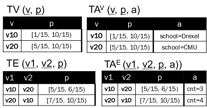
Figure 4: node${}^{T}_{a}(school,set(school),max(cnt).)$

The node creation operator enables the user to analyze an evolving graph at different levels of granularity. This operator comes in two variants — based on vertex attributes or based on temporal window.

Attribute-based node creation is denoted
$\textsf{node}^{T}_{a}(g_{1},\ldots,g_{i},f_{v1}(k_{1}),\ldots,f_{vn}(k_{n}),f_{e1}(l_{1}),\ldots,f_{em}(l_{m}),\mathsf{T})$, where $g_{1},\ldots,g_{i}$ are the grouping attributes, and each $f_{vj}(k_{j})$ ($f_{ej}(l_{j})$) specifies an aggregation function $f_{vj}$ (resp. $f_{ej}$) to be applied to a vertex property $k_{j}$ (resp. edge property $l_{j}$). This operation allows the user to generate a TGraph in which vertices correspond to disjoint groups of vertices in the input that agree on the values of all grouping attributes. For example, $\textsf{node}^{T}_{a}(school,\mathsf{T})$ will compute a vertex for each value of $\mathsf{TA^{V}}.a.school$. Vertices that do not specify a value for one or several grouping attributes at a given time, will not contribute to the result for the corresponding snapshot.

To compute $\mathsf{T}^{\prime}=\textsf{node}^{T}_{a}(g_{1},\ldots,g_{i},f_{v1}(k_{1}),\ldots,f_{vn}(k_{n}),$
$f_{e1}(l_{1}),\ldots,f_{em}(l_{m}),\mathsf{T})$, we execute $L=g_{1},\ldots,g_{i}\gamma^{T}(\textsf{TV}\mathbin{\Join\mkern-5.8mu\rule[0.86108pt]{2.5pt}{0.4pt}\hbox to0.0pt{\hss\rule[6.45831pt]{2.5pt}{0.4pt}}}^{T}_{v}\mathsf{TA^{V}})$, computing an intermediate temporal relation for each group. Next, we generate the new vertex relation $\textsf{TV}^{\prime}$, by generating an id for each group with a Skolem function: $\textsf{TV}^{\prime}=\sigma^{T}_{skolem(g_{1},\ldots,g_{i})}L$.

Then, $\mathsf{TA^{V}}^{\prime}=\mathcal{R}(f_{v1}(k_{1}),\ldots,f_{vn}(k_{n}),\sigma^{T}_{skolem(g_{1},\ldots,g_{i}),a}L)$. Note the use of the resolve primitive to reconcile attribute values within a group.

Vertices of the input are partitioned on their values of the grouping attributes. Partitioning of the vertices also induces a partitioning of the edges. To compute the new edges $\textsf{TE}^{\prime}$, we generate a temporal conjunctive query that computes $E(v_{1},v_{2},p,v_{1}^{\prime},v_{2}^{\prime})$, where $v_{1}^{\prime}$ and $v_{2}^{\prime}$ are the identifiers of the vertices in TV’ to which $v_{1}$ and $v_{2}$ are mapped. Finally, we compute $\textsf{TE}^{\prime}=\mathcal{C}(\pi^{T}_{v_{1}^{\prime},v_{2}^{\prime}}E)$ and
$\mathsf{TA^{E}}^{\prime}=\mathcal{R}(f_{e1}(l_{1}),\ldots,f_{vm}(l_{m}),v_{1}^{\prime},v_{2}^{\prime}\gamma^{T}(E\bowtie^{T}_{v_{1},v_{2}}\mathsf{TA^{E}}))$.

Figure 4 illustrates attribute-based node creation over T1 in our running example, with set(school) aggregation function for vertices and and max(cnt) for edges. Vertices $v_{1}$ and $v_{3}$ create a single new vertex $v_{10}$, representing Drexel.

Window-based node creation is denoted
$\textsf{node}^{T}_{w}(w,q_{v},q_{e},f_{v1}(k_{1}),\ldots,f_{vn}(k_{n}),f_{e1}(l_{1}),\ldots,f_{em}(l_{m}),\mathsf{T})$, where $w$ is the window specification, $q_{v}$ and $q_{e}$ are vertex and edge quantifiers, and each $f_{vj}(k_{j})$ ($f_{ej}(l_{j})$) specifies an aggregation function $f_{vj}$ (resp. $f_{ej}$) to be applied to a vertex property $k_{j}$ (resp. edge property $l_{j}$). This operation corresponds to moving window temporal aggregation, and is inspired by the stream aggregation work of [28] and by generalized quantifiers of [19], both adopted to graphs.

Window specification $w$ is of the form $n~{}\{unit|\textsf{changes}\}$, where $n$ is an integer, and $unit$ is a time unit, e.g., $10~{}min$, $3~{}years$, or any multiple of the usual time units. When $w$ is the form $n~{}\textsf{changes}$, it defines the window by the number of changes that occurred in $\mathsf{T}$ (affecting any of its constituent relations). Window boundaries are computed left-to-right, i.e., from least to most recent.

Vertex and edge quantifiers $q_{v}$ and $q_{e}$ are of the form { all | most | at least $n$ | exists }, where $n$ is a decimal representing the percentage of the time during which a vertex or an edge existed, relative to the duration of the window (exists is the default). Quantifiers are useful for observing different kinds of temporal evolution, e.g., to observe only strong connections over a volatile evolving graph, we may want to only include vertices that span the entire window ($q_{v}=\textsf{all}$), and edges that span a large portion of the window ($q_{e}=\textsf{most}$).

For both kinds of window specification (by unit or by number of changes), we must (1) compute a mapping from a tuple in a temporal relation to one or multiple windows, and (2) aggregate over each window. The $s$ parameter for the split primitive is the smallest start date across $\mathsf{T}$.

To compute $\textsf{TV}^{\prime}$, we apply split to TV, group by vid, select only those vertices that meet the quantification, and finally coalesce: $\textsf{TV}^{\prime}=\mathcal{C}(\sigma^{T}_{q_{V}}(v\gamma^{T}_{\cup p}(\mathcal{S}(s,w,\textsf{TV}))))$. Similarly for $\textsf{TE}^{\prime}$. To compute attribute relations we split, resolve with the aggregation functions, and constrain: $\mathsf{TA^{V}}^{\prime}=\mathcal{K}(\mathcal{R}(f_{v1}(k_{1}),\ldots,f_{vn}(k_{n}),\mathcal{S}(s,w,\mathsf{TA^{V}})),\textsf{TV}^{\prime})$, similarly for $\mathsf{TA^{E}}^{\prime}$.

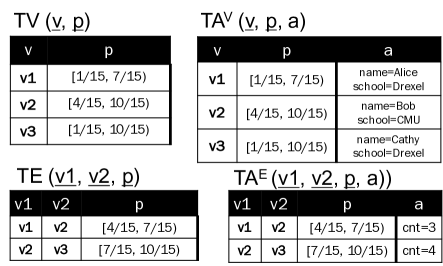
(a) By time: $w=3~{}\textsf{months}$.

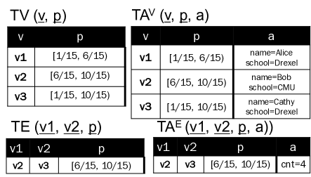
(b) By change: $w=3~{}\textsf{changes}$.

Figure 5: Node creation, $\textsf{node}^{T}_{w}(\mathsf{q_{v}=always},\mathsf{q_{e}=exists,f_{v}=\{first(name),~{}first(school)\}},\mathsf{T})$.

Figure 5(a) illustrates window-based node creation by time ($w=3~{}\textsf{months}$), and Figure 5(b) — by change ($w=3~{}\textsf{changes}$). Both are applied to T1 in our running example with all quantifier for vertices and exists for edges, and first aggregation function for vertex and edge properties. $v_{2}$ is present in the result in Figure 5(a) starting at $4/15$ because it did not exist for the entirety of the first window, while in Figure 5(b) it is produced starting $6/15$.

3.6 Edge creation

Edge creation $\textsf{edge}^{T}(q,f_{1}(k_{1}),\ldots,f_{n}(k_{n}),\mathsf{T}_{1},\mathsf{T}_{2})$ is a binary operator that computes a TGraph on the vertices $\textsf{TV}=\textsf{TV}_{1}\cup^{T}\textsf{TV}_{2}$, with edges and edge attributes computed by a conjunctive query over the constituent relations of $\mathsf{T}_{1}$ and $\mathsf{T}_{2}$. $L(v_{1},v_{2},a,p)=\mathcal{R}(f_{1}(k_{1}),\ldots,f_{n}(k_{n}),q(\mathsf{T}_{1},\mathsf{T}_{2}))$, and then set $\textsf{TE}^{\prime}=\mathcal{C}(\pi^{T}_{v1,v2}L)$, and $\mathsf{TA^{E}}^{\prime}=\sigma_{a~{}is~{}not~{}null}L$. We then compute $\mathsf{TA^{V}}=\mathcal{R}(f_{1}(k_{1}),\ldots,f_{n}(k_{n}),\textsf{TV}_{1}\cup^{T}\textsf{TV}_{2})$.

Edge creation has several important applications. It can be used to compute friend-of-friend edges (passing in the same TGraph as both arguments). Since $q$ can include predicates over the timestamps, $\textsf{edge}^{T}$ can compute journeys. A journey is a path in the evolving graph with non-decreasing time edges [8, 13]. By adding a temporal condition to $q$, we can obtain journeys similar to time-concurrent paths.

In graph theory, a graph join of two undirected unlabeled disjoint graphs is defined as the union of the two graphs and additional edges connecting every vertex in graph one with each vertex in graph two. We can obtain a graph join by computing $\textsf{TE}^{\prime}=\textsf{TV}_{1}\times^{T}\textsf{TV}_{2}$.

SocialScope [3] defines (non-temporal) graph composition: compose the edge of the two operands and return an edge-induced subgraph. TGA can express this operator by a combination of edge creation and vertex subgraph.

3.7 Extension: user-defined analytics

For many types of analysis, it is necessary to compute some property, such as PageRank of each vertex $v$, or the length of the shortest path from a given designated vertex $u$ to each $v$, for each time point. This information can then be used to study how the graph evolves over time. Portal supports this type of analysis through temporal user-defined analytics, which conceptually execute an aggregation-map operation sequence repeatedly over a set number of iterations or until fix-point and save the result in property $pname$. $\mathsf{T}^{\prime}=\textsf{pregel}^{T}(dir,cond,f_{m},f_{a},pname,iter,\mathsf{T})$, where all arguments are like in aggregation, with an additional $iter$ argument specifying the number of iterations to perform.

4 Expressive power

In this section we study expressiveness of the TGraph model, which consists of the TGraph data structure (Definition 2.1) and of TGA, an algebra for querying the data structure (Section 3). We stress that ours is a valid-time data model that does not provide transaction-time and bi-temporal support.

Important note: We restrict our attention to a subset of TGA operations, excluding window-based node creation (Section 3.5) from our analysis. Window-based node creation requires the split $\mathcal{S}(s,w,R)$ primitive, which cannot be naturally expressed in TRA. We defer an investigation of expressiveness of TGA with window-based node creation to future work.

We start by proposing two natural notions of completeness for a temporal graph query language.

Definition 4.1

Let $L^{t}$ be a temporal relational language and $\mathsf{T}$ — a relational representation of a temporal graph. An edge-query $q^{t}_{e}$ in $L$ takes a graph $\mathsf{T}(\textsf{TV},\textsf{TE},\mathsf{TA^{V}},\mathsf{TA^{E}})$ as input, and outputs another graph $\mathsf{T}^{\prime}$ on the vertices of $\mathsf{T}$ such that the edges of $\mathsf{T}^{\prime}$ are defined by $q^{t}_{e}$. A language is $L^{t}$-edge-complete if it can express each $q^{t}_{e}$ in $L^{t}$.

Note that the query $q^{t}_{e}$ is not restricted to act on TE alone, and may refer to the other constituent relations $\mathsf{T}$.

Definition 4.2

Let $L^{t}$ be a temporal relational language, and let $\mathsf{T}$ be a relational representation of a temporal graph. A vertex-query $q^{t}_{v}$ in $L^{t}$ takes a graph $\mathsf{T}(\textsf{TV},\textsf{TE},\mathsf{TA^{V}},\mathsf{TA^{E}})$ as input, and outputs another graph $\mathsf{T}^{\prime}$ such that the vertices of $\mathsf{T}^{\prime}$ are defined by $q^{t}_{v}$. A language is $L^{t}$-vertex-complete if it can express each $q^{t}_{v}$ in $L^{t}$.

We now refer to definitions 4.1 and 4.2 and show that TGA is edge-complete and vertex-complete, with respect to the valid-time fragment of temporal relational algebra (TRA). TRA is an algebra that corresponds to temporal relational calculus [11], a first-order logic that extends relational calculus, supporting variables and quantifiers over both the data domain and time domain.

Theorem 1

TGA is TRA-edge-complete.

Proof 4.2.

The result of every conjunctive edge-query over the vertices of $\mathsf{T}$ can be expressed by $\sigma_{c}(\textsf{TV}\times^{T}\textsf{TV})$. Queries of this kind can be expressed by the edge creation operator of TGA (Section 3.6), invoked as:
$\textsf{edge}^{T}(q=\sigma_{c}(\mathsf{T}_{1}.\textsf{TV}\times^{T}\mathsf{T}_{2}.\textsf{TV}),\mathsf{T}_{1}=\mathsf{T},\mathsf{T}_{2}=\mathsf{T})$

Theorem 4.3.

TGA is TRA-vertex-complete.

Proof 4.4.

Every TRA vertex-query can be expressed in TGA by a sequence of vertex-subgraph $q^{T}_{v}(\mathsf{T})$ (Section 3.2) and attribute-based node creation $\textsf{node}^{T}_{a}$ (Section 3.5). Attribute-based node creation supports Skolem functions, and is necessary to handle queries that introduce vertex identifiers.

For a point-based model, it is customary to interrogate two properties — snapshot reducibility (S-reducibility) and extended snapshot reducibility (extended S-reducibility). S-reducibility states that for every query $q$ in $L$, there must exist a syntactically similar query $q^{t}$ in $L^{t}$ that generalizes $q$. Specifically the following relationship should hold when $q^{t}$ is evaluated over a temporal database $D^{t}$ (recall that $\tau$ is the temporal slice operator): $q(\tau_{c}(D^{t}))=\tau_{c}(q^{t}(D^{t}))$, for all time points $c$. Extended S-reducibility requires that $L^{t}$ provide an ability to make explicit references to timestamps alongside non-temporal predicates.

TGA is s-reducible and extended s-reducible because, as we showed in Section 3, every TRA operation can be rewritten into TRA, which is s-reducible and extended s-reducible w.r.t. relational algebra.

5 System

We developed a prototype system Portal which supports TGA operations on top of Apache Spark/GraphX [18]. The data is distributed in partitions across the cluster workers, read in from HDFS, and can be viewed both as a graph and as a pair of RDDs. All TGraph operations are available through the public API of the Portal library, and may be used in an Apache Spark application.

5.1 Reducing temporal operators

Apache Spark is not a temporal DBMS but rather an open-source in-memory distributed framework that combines graph parallel and data parallel abstractions. Following the approach of Dignos et al. [12] we reduce our temporal operators into a sequence of nontemporal relational operators or their equivalents for Spark RDDs, maintaining point semantics. This allows our algebra to be implemented in any nontemporal relational database. In total, we need the four temporal primitives we introduced in Section 3.1 (coalesce, resolve, constrain, and split), as well as the primitives described in [12]: extend and normalize. Because our model uses point semantics and does not require change preservation, we do not need the align primitive of [12] and can use the normalize primitive in its place.

The coalesce primitive merges adjacent and overlapping time periods for value-equivalent tuples. This operation, which is similar to duplicate elimination in conventional databases, has been extensively studied in the literature [5, 38]. Several implementations are possible for the coalesce operation over temporal SQL relations. Because Spark is an in-memory processing system, we use the partitioning method, where the relation is grouped by key, and tuples are sorted and folded within each group to produce time periods of maximum length. Eager coalescing, however, is not desirable since it is expensive and some operations may produce correct results (up to coalescing) even when computing over uncoalesced inputs. Any operation that is time-variant requires input to be coalesced. We base the eager coalescing rules on coalescing rules in TRA [5].

The resolve primitive is implemented using a group by key operation in Spark and convenience methods on the property set class. The property set class supports adding all properties from another set such that they are combined by key, and applying aggregation functions one at a time for each property name.

The constrain primitive constrains one relation with respect to another, such as removing edges from the result that do not have associated nodes, or trimming the edge validity period to be within the validity periods of associated nodes. It is introduced here because Spark does not have a built-in way to express foreign key constraints. We do this by executing a join of the two relations — either a broadcast join or a hash join — and then adjusting time periods as necessary. This is an expensive operation and is only performed when necessary as determined by the soundness analysis, e.g., when vertex-subgraph has a non-trivial predicate over $\mathsf{T}$, and when node creation has a more restrictive vertex quantifier $q_{v}$ than edge quantifier $q_{e}$.

The split primitive maps each tuple in relation $R$ into one or more tuples based on a temporal window expression such as w=3 months. A purely relational implementation of this primitive is possible with the use of a special Chron relation that stores all possible time points of the temporal universe and supports computation without materialization. Another approach is to introduce fold and unfold functions that can split each interval into all its constituent time points. Both of these approaches have strong efficiency concerns, see [7] for an in-depth discussion. In Spark we are not limited to relational operators only and can use functional programming constructs. Split can be efficiently implemented with a flatMap, which emits multiple tuples as necessary by applying a lambda function and flattening the result. We use this method in our implementation.

The extend primitive extends a relation with an additional attribute that represents the tuple’s timestamp, see [12] for a definition. Extend allows explicit references to timestamps in operations, and is needed for extended snapshot reducibility. We implement extend by defining an Interval class and including it as a field in every RDD.

The normalize primitive produces a set of tuples for each tuple in r by splitting its timestamp into non-overlapping periods with respect to another relation s and attributes B. See [12] for the formal definition. Intuitively, normalize creates tuples in corresponding groups such that their timestamps are also equivalent. This primitive is necessary for node creation, set operators like union, and joins. Normalize primitive relies on an efficient implementation of the tuple splitter. We split each tuple based on the change periods over the whole graph, avoiding costly joins but potentially splitting some tuples unnecessarily.

5.2 Physical Representations

It is convenient to use intervals to compactly represent consecutive value-equivalent snapshots of $\mathsf{T}$— timeslices in which no change occurred in graph topology, or in vertex and edge attributes. We use the term representative graph to refer to such snapshots, since they represent an interval.

We considered four in-memory TGraph representations that differ both in compactness and in the kind of locality they prioritize. With structural locality, neighboring vertices (resp. edges) of the same representative graph are laid out together, while with temporal locality, consecutive states of the same vertex (resp. edge) are laid out together [29]. We now describe each representation.

We can convert from one representation to any other at a small cost (as supported by our experimental results), so it is useful to think of them as access methods in the context of individual operations.

VertexEdge (VE) is a direct implementation of the $\mathsf{T}$ model, and is the most compact: one RDD contains all vertices and another all edges. Consistently with the GraphX API, all vertex properties are stored together as a single nested attribute, as are all edge properties. We currently do not store the TV and TE relations separately but rather together with $\mathsf{TA^{V}}$ and $\mathsf{TA^{E}}$, respectively. While VE does not necessitate a particular order of tuples on disk, we opt for a physical layout in which all tuples corresponding to the same vertex (resp. edge) are laid out consecutively, and so VE preserves temporal locality.

VE supports all TGA operations except analytics, because an analytic is defined on a representative graph, which VE does not materialize. As we will show in Section 6, this physical representation is the most efficient for many operations. In the current prototype we limit the expressiveness of some of the operations, such as only supporting vertex- and edge-subgraph queries over the $\mathsf{TA^{V}}$ and $\mathsf{TA^{E}}$ relations.

RepresentativeGraphs (RG) is a collection (parallel sequence) of GraphX graphs, one for each representative graph of $\mathsf{T}$, where vertices and edges store the attribute values for the specific time interval, thus using structural locality. This representation supports all operations of TGA which can be expressed over snapshots, i.e. any operation which does not explicitly refer to time. GraphX provides Pregel API which is used to support all the analytics. While the RG representation is simple, it is not compact, considering that in many real-world evolving graphs there is a 80% or larger similarity between consecutive snapshots [29]. In a distributed architecture, however, this data structure provides some benefits as operations on it can be easily parallelized by assigning different representative graphs to different workers. We include this representation mainly as a naive implementation to compare performance against.

RG is the most immediate way to implement evolving graphs using GraphX. Without Portal a user wishing to analyze evolving graphs might implement and use the RG approach. However, as we will show in Section 6, this would lead to poor performance for most operations.

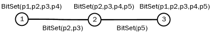
Figure 6: OG representation of T1.

OneGraph (OG) is the most topologically compact representation, which stores all vertices from $\mathsf{TA^{V}}$and edges from $\mathsf{TA^{E}}$ once, in a single aggregated data structure. OG emphasizes temporal locality, while also preserving structural locality, but leads to a much denser graph than RG. This, in turn, makes parallelizing computation challenging.

An OG is implemented as a single GraphX graph where the vertex and edge attributes are bitsets that encode the presence of a vertex or edge in each time period associated with some representative graph of a TGraph. To construct an OG from $\mathsf{T}$, vertices and edges of TV and TE relations each are grouped by key and mapped to bits corresponding to periods of change over the graph. Because OG stores information only about graph topology, far fewer periods must be represented and computed for OG than for RG. The actual reduction depends on the rate and nature of graph evolution. Information about time validity is stored together with each vertex and edge. Figure 6 shows the OG for T1 from Figure 1.

Analytics are supported using a batching method over the Pregel API. Similar to ImmortalGraph [29], the analytics are computed over all the representative graphs together. Vertices exchange messages marked with the applicable intervals and a single message may contain several interval values as necessary.

As we will see experimentally in Section 6, OG is often the best-performing data structure for node creation, and also has competitive performance for analytics. Because of this focus, OG supports operations only on topology: analytics, node creation. and set operators for graphs with no vertex or edge attributes. All other operations are supported through inheritance from an abstract parent, and are carried out on the VE data structure. Thus OG and HG, below, can be thought of as indexes on VE.

In our preliminary experiments we observed that OG exhibited worse than expected performance, especially for large graphs with long lifetimes. The reason this is so is because good graph partitioning becomes difficult as topology changes over time. Communication cost is the main contributor to analytics performance over distributed graphs, so poor partitioning leads to increased communication costs. When the whole graph can fit into memory of a single worker, communication cost goes away and the batching method used by OG becomes the most efficient, as has been previously shown in [29]. To provide better performance on analytics, we introduce HybridGraph (HG). HG trades compactness of OG for better structural locality of RG, by aggregating together several consecutive representative graphs, computing a single OG for each graph group, and storing these as a parallel sequence. In our current implementation each OG in the sequence corresponds to the same number of temporally adjacent graphs. This is the simplest grouping method, and we observed that placing the same number of graphs into each group often results in unbalanced group sizes. This is because evolving graphs commonly exhibit strong temporal skew, with later graphs being significantly larger than earlier ones. We are currently working on more sophisticated grouping approaches that would lead to better balance, and ultimately to better performance. However as we will see experimentally in Section 6, the current HG implementation already improves performance compared to OG, in some cases significantly.

Like OG, HG focuses on topology-based analysis, and so does not represent vertex and edge attributes. HG implements analytics, node creation, and set operators, and supports all other operations through inheritance from VE. Analytics are implemented similar to OG, with batching within each graph group.

Since RG, OG and HG are implemented over GraphX graphs, the referential integrity is maintained by the framework and the constrain primitive is not required. All primitives are used with the VE representation.

5.3 Additional Implementation Details

Partitioning. Graph partitioning has a tremendous impact on performance. A good partitioning strategy needs to be balanced, assigning an approximately equal number of units to each partition, and limit the number of cuts across partitions, reducing cross-partition communication. In previous experiments we compared performance with no repartitioning after load vs. with repartitioning, using the GraphX E2D edge partitioning strategy. In E2D, a sparse edge adjacency matrix is partitioned in two dimensions, guaranteeing a $2\sqrt{n}$ bound on vertex replication, where $n$ is the number of partitions. E2D has been shown to provide good performance for Pregel-style analytics [18, 37]. The user can repartition the representations at will, consistent with the Spark approach.

Graph loading. We use the Apache Parquet format for on-disk storage, with one archive for vertices and another for edges, temporally coalesced. This format corresponds to the VE physical representation 5.2. In cases where there is no more than 1 attribute per vertex and edge, this representation is also the most compact.

For ease of use, we provide a GraphLoader utility that can initialize any of the four physical representations from Apache Parquet files on HDFS or on local disk. A Portal user can also implement custom graph loading methods to load vertices and edges, and then use the fromRDDs to initialize any of the four physical representations.

Integration with SQL. The Portal API exposes vertex/edge RDDs to the user and provides convenience methods to convert them to Spark Datasets. Arbitrary SparkSQL queries can then be executed over these relations.

6 Experimental Evaluation

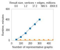
Figure 7: Slice on nGrams.

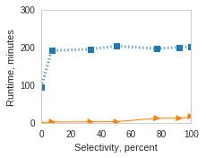
Figure 8: Subgraph on nGrams.

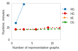
Figure 9: Aggregate on Twitter.

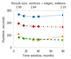
(a) $q_{v}=\textsf{always}$, $q_{e}=\textsf{always}$, wiki-talk

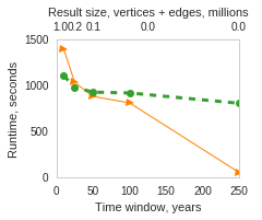
(b) $q_{v}=\textsf{always}$, $q_{e}=\textsf{exists}$, nGrams

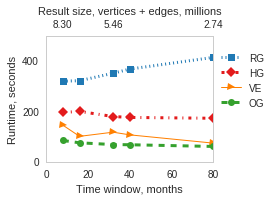
(c) $q_{v}=\textsf{always}$, $q_{e}=\textsf{exists}$, wiki-talk

Figure 10: Node creation with temporal windows.

6.1 Setup

All experiments were conducted on a 16-slave in-house Open Stack cloud, using Linux Ubuntu 14.04 and Spark v2.0. Each node has 4 cores and 16 GB of RAM. Spark Standalone cluster manager and Hadoop 2.6 were used. Because Spark is a lazy evaluation system, a materialize operation was appended to the end of each query, which consisted of the count of nodes and edges. Each experiment was conducted 3 times with a cold start – the running time includes the setup time of submitting the job to the cluster manager, uploading the jar to the cluster, reading the data from disk, building the chosen representation, and running a single query. We report the average running time, which is representative because we took great care to control variability: standard deviation for each measure is at or below 5% of the mean except in cases of very small running times. No computation results were shared between subsequent runs.

Data. We evaluate performance of our framework on three real open-source datasets, summarized in Table 1. wiki-talk (http://dx.doi.org/10.5281/zenodo.49561) contains over 10 million messaging events among 3 million wiki-en users, aggregated at 1-month resolution.
nGrams (http://storage.googleapis.com/books/ngrams/books/datasetsv2.html) contains word co-occurrence pairs, with 30 million word nodes and over 2.5 billion undirected edges. The Twitter social graph [14] contains over 23 billion directed follower relationships between 0.5 billion twitter users, sampled at 1-month resolution. The datasets differ in size, in the number and type of attributes and in evolution rates, calculated as the average graph edit similarity [30].

6.2 Individual operators

Slice performance was evaluated by varying the slice time window and materializing the TGraph, and is presented in Figures 9 for nGrams and 20 for wiki-talk (in Appendix B). Similar trends were observed for twitter. Slice is expected to be more efficient when executed over VE when data is coalesced on disk than over RG, and we observe this in our experiments. This is because multiple passes over the data are required for RG to compute each representative graph, leading to linear growth in running times for file formats and systems without filter pushdown, as is the case here. Slice over VE simply executes temporal selection and has constant running times (29 sec for wiki-talk, about 1.5 min for nGrams). This experiment essentially measures the cost of materializing RG from its on-disk representation.

Vertex subgraph performance was evaluated by specifying a condition on the $length(a.attr)<t$ of the vertex attribute, with different values of $t$ leading to different selectivity. This experiment was executed for wiki-talk (with $username$ as the property) and for nGrams (with $word$ as the property). Twitter has no vertex attributes and was not used in this experiment. Figure 9 shows performance for RG and VE on nGrams (wiki-talk results in Appendix B). Performance on RG is a function of the number of intervals and is insensitive to the selectivity. The behavior on VE is dominated by FK enforcement: with high selectivity (few vertices) broadcast join affords performance linear in the number of edges, whereas for a large number of vertices broadcast join is infeasible and a hash-join is used instead, which is substantially slower. VE provides an order of magnitude better performance than RG: up to 3 min with hash-join and up to 15 min with broadcast join for VE, in contrast to between 95 and 200 min for RG.

Map exhibits a similar trend as slice: constant running time for VE and a linear increase in running time with increasing number of representative graphs for RG (Figure 20 for wiki-talk in Appendix B, similar for other datasets). Performance of map is slightly worse than that of slice because map must coalesce its output as the last step, while slice does not.

Table 1: Experimental datasets.

Dataset	|V|	|E|	Time Span	Evol. Rate
wiki-talk-en	2.9M	10.7M	2002–2015	14.4
nGrams	29.3M	2.5B	1520–2008	16.67
twitter	505.4M	23B	2006–2012	88

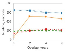
Figure 11: Union on wiki-talk.

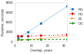
Figure 12: Intersection on nGrams.

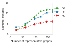
Figure 13: Components on wiki-talk.

Aggregation performance was evaluated on the graph-based representations with a computation of vertex degrees, varying the size of the temporal window obtained with slice. The results in Figure 9 indicate that materialization of each representative graph required for RG makes it not a viable candidate for this operation, especially over large datasets. Both OG and HG exhibit linear increase in performance as the slice size is increased, with a small slope. Similar performance was observed in the other datasets.

Node creation performance was evaluated on all representations, since all have different implementations of this operator. We executed topology-only creation (no attributes), varying the size of the temporal window. We observe that performance depends heavily on the quantification, and on the data evolution rate. OG is an aggregated data structure with good temporal locality and thus in most cases provides good performance and is insensitive to the temporal window size (Figure 10(a)). However, in datasets with a large number of representative graphs (such as nGrams), OG is slow on large windows, an order of magnitude worse than VE in the worst case (Figure 10(b)). VE outperforms OG when vertex and edge quantification levels match (Figure 10(a)), but is worse than OG when vertex quantification is stricter than edge quantification and FK must be enforced (Figure 10(c)). OG also outperforms VE when both evolution rate is low and aggregation window is small (Figure 10(a), wiki-talk).

Union, intersection, and difference by structure were evaluated by loading two time slices of the same dataset with varying temporal overlap. Performance depends on the size of the overlap (in the number of representative graphs) and on the evolution rate. VE has best performance when overlap is small (Figure 13). OG always has good performance, constant w.r.t. overlap size. This is expected, since OG union and intersection are implemented as joins (outer or inner) on the vertices and edges of the two operands. VE, on the other hand, splits the coalesced vertices/edges of each of the two operands into intervals first, takes a union, and then reduces by key. When evolution rate is low and duration of an entity is high, such as in wiki-talk for vertices, the split produces a lot of tuples to then reduce, and performance suffers (Figure 13). RG only has good performance on intersection when few representative graphs overlap, and never on union (Figure 13). HG performance is worse than OG, by a constant amount in union, and diverges in intersection.

Analytics. We implemented PageRank (PR) and Connected Components (CC) analytics for the three graph-based representations using the Pregel GraphX API. PR was executed for 10 iterations or until convergence, whichever came first. CC was executed until convergence with no limit on the number of iterations. Performance of Pregel-based algorithms depends heavily on the partitioning strategy, with best results achieved where cross-partition communication is small [37]. For this reason, we evaluated only with the E2D strategy. Performance was evaluated on time slices of varying size. Recollect that analytics are essentially multiple rounds of aggregate operations, so the performance we observe is an amplified version of aggregate performance. For a very small number of graphs (1-2), RG provides good performance, but slows down linearly as the number of graphs increases. HG provides the best performance on analytics under most conditions, with a linear increase but a significantly slower rate of growth. The tradeoff between OG and HG depends on graph evolution characteristics. If the graph is a growth-only evolution (such as in Twitter), OG is not denser than HG and computes everything in a single batch, which leads to the fastest performance, as can be seen in Figure 23. If the edge evolution represents more transient connections, then HG is less dense and scales better (Figure 13). Note that OG and HG performance could be further improved by computing them over coalesced structure-only V and E, and ignoring attributes.

In summary, no one data structure is most efficient across all operations. This opens the door to query optimization based on the characteristics of the data such as graph evolution rate and on the type of operation being performed.

6.3 Switching between representations

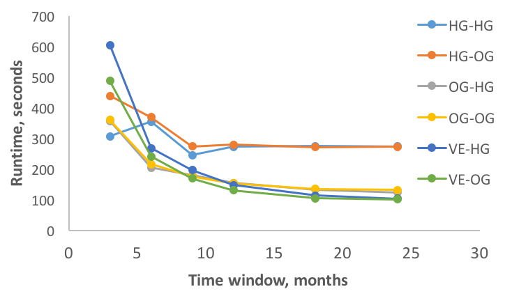
Figure 14: $\textsf{node}^{T}_{a}$ followed by components.

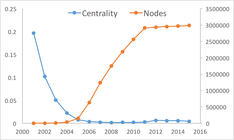
Figure 15: In-degree centrality with 1 year resolution.

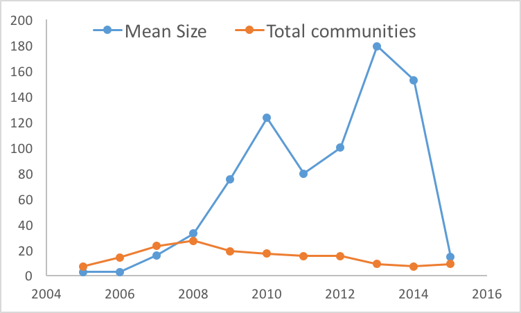
Figure 16: Communities with 1 year resolution.

To treat the four representations as access methods, we need to be able to switch between them. The data structures can be created from outputs of any of the four, at a cost. To investigate the feasibility of switching between representations, we executed two-operator queries and either kept the representation constant or changed it between the operators. The query is based on the first two steps of example three in our motivating use cases: node creation over temporal windows in wiki-talk, followed by the connected components analytic. Figure 16 shows the result of varying the size of the temporal window. Recall that OG is the best performing representation for node creation at small windows and HG for components over this dataset. The benefits of HG are substantially consumed by switching: the performance of OG-OG and and OG-HG are similar. If the cost of switching was negligible, then OG-HG should have exhibited notably better performance than all other combinations. However, the OG-HG still performs best over-all, indicating that switching is feasible.

6.4 Use cases

To see how our algebra handles the use cases from Section 1.1, we implemented each one over the wiki-talk dataset. Each example requires a sequence of operators. For each operator we used the best performing data structures based on the comparison experiments described above.

Example 1 answers the question of whether there are high influence nodes and whether that behavior is persistent in time. The code to compute the answer is 4 lines of a Scala program and the query took 76 seconds to execute. The results show that from 25 nodes with mean degree of 40 and above that have persisted for at least 6 months, 6 have coefficient of variation below 50, which is quite low, and only 5 have it above 100. This indicates that there are in fact high in-degree nodes and that they continue to be influential over long periods of time, despite the loose connectivity of the overall network.

Example 2 examines how the graph centrality changes over time. The program is 6 lines of Scala code iterating with temporal windows of 1, 2, 3, 6, and 12 months, and the analysis took 25 minutes. Results show that regardless of the temporal resolution, the in-degree centrality is extremely low, about 0.04. Figure 16 provides an explanation – as the size of the graph increases, its centrality decreases. Given that the number of edges in this graph is only about 4 times the number of nodes, the graph is too sparse and disjointed to have any centrality.

Finally, example 3 examines whether communities can be detected in the wiki-talk network at different temporal resolution. The program, similar to the one above, is 6 lines of Scala code with varied temporal windows. The total runtime is 58 minutes. Communities, defined as connected components, can be detected in all temporal resolutions. As a reminder, the edge quantification in this query is always, so only edges that persist over each window are retained. The presence of communities even with large temporal resolution indicates that communities form and persist over time. Figure 16 shows the mean size of all communities by time and their total number. The peaks of the mean size, visible in all temporal windows, may indicate that communities form and then reform in a different configuration, perhaps for a different purpose. The results of this analysis can serve as a starting point to investigate the large communities and what caused the size shifts.

In summary, complex analyses can be expressed as queries in Portal and lead to interesting insights about the evolution of the underlying phenomena.

7 Related Work

Evolving graph models. Much recent work represents evolving graphs as sequences of snapshots in a discrete time domain, and focuses on snapshot retrieval and analytics [23, 29, 30]. Our logical model is semantically equivalent to a sequence of snapshots because in point semantics snapshots can be obtained with a simple slice over all time points. We choose to represent TGraphs as a collection of vertices and edges because the range of operations we support is naturally expressible over them but not over a sequence of snapshots. For example, subgraph with a temporal predicate is impossible to express over snapshot sequences as each snapshot is nontemporal and independent of the others.

Querying and analytics. There has been much recent work on analytics for evolving graphs, see [2] for a survey. This line of work is synergistic with ours, since our aim is to provide systematic support for scalable querying and analysis of evolving graphs.

Several researchers have proposed individual queries, or classes of queries, for evolving graphs, but without a unifying syntax or general framework. The proposed operators can be divided into those that return temporal or nontemporal result. Temporal operators include retrieval of version data for a particular node and edge [16], of journeys [15, 8], subgraph by time or attributes [20, 24], snapshot analytics [29, 26, 24], and computation of time-varying versions of whole-graph analytics like maximal time-connected component [13] and dynamic graph centrality [27]. Non-temporal operators include snapshot retrieval [23] and retrieval at time point [15, 24].

Our contribution is to propose one unifying compositional TGA that covers the range of the operations in a complete way, with clear semantics, which many previous works lack.

Implementations. Three systems in the literature focus on systematic support of evolving graphs, all of them non-compositional. Miao et al. [29] developed ImmortalGraph (formerly Chronos), a proprietary in-memory execution engine for temporal graph analytics. The ImmortalGraph system has no formal model, but informally an evolving graph is defined as a series of activities on the graph, such as node additions and deletions. This is a streaming or delta approach, which is popular in temporal databases because it is unambiguous and compact. ImmortalGraph does not provide a query language, focusing primarily on efficient physical data layout. Many insights about temporal vs. structural locality by [29] hold in our setting. The batching method for snapshot analytics used by OG is similar to the one proposed in ImmortalGraph. However, ImmortalGraph was developed with the focus on centralized rather than distributed computation and [29] does not explore the effect of distribution on batching performance.

The G* system [26] manages graphs that correspond to periodic snapshots, with the focus on efficient data layout. It takes advantage of the similarity between successive snapshots by storing shared vertices only once and maintaining per-graph indexes. Time is not an intrinsic part of the system, as there is in TGA, and thus temporal queries with time predicates like node creation are not supported. G* provides two query languages: procedural query language PGQL, and a declarative graph query language (DGQL). PGQL provides graph operators such as retrieving vertices and their edges from disk and non-graph operators like aggregate, union, projection, and join. All operators use a streaming model, i.e. like in traditional DBMS, they pipeline. DGQL is similar to SQL and is converted into PGQL by the system.

Finally, the Historical Graph Store (HGS) system is an evolving graph query system based on Spark. It uses the property graph model and supports retrieval tasks along time and entity dimensions through Java and Python API. It provides a range of operators such as selection (equivalent to our subgraph operators but with no temporal predicates), timeslice, nodecompute (similar to map but also with no temporal information), as well as various evolution-centered operators. HGS does not provide formal semantics for any of the operations it supports and the main focus is on efficient on-disk representation for retrieval.

None of the three systems are publicly available, so direct performance comparison with them is not feasible.

8 Conclusions and Future Work

In this paper we presented TGA: a tuple-stamped vertex and edge relational model of evolving graphs and a rich set of operations with point semantics. TGA is TRA-vertex- and -edge-complete. We show reduction of each of our operations into TRA and further into RA with additional primitives.

It is in our immediate plans to develop a declarative syntax for TRA, making it accessible to a wider audience of users. We described an implementation of Portal in scope of Apache Spark, and studied performance of operations on different physical representations. Interestingly, different physical implementations perform best for different operations but support switching, opening up avenues for rule-based and cost-based optimization. Developing a query optimizer for Portal is in our immediate plans.

Appendix A Additional examples.

Figure 17(a) shows the result of temporal intersection of T1 with T2. Only the vertices and edges present in both TGraphs are produced, thus eliminating $v_{3}$ and $v_{4}$. Period $[2/15,4/15)$ for $v_{2}$ is computed as a result of the join of $[2/15,5/15)$ in T1 and [$2/15,4/15)$ in T2.

Figure 17(b) shows the result of temporal difference of T1 with T2. Vertex v1 is removed between 2/15 and 6/15, splitting one v1 tuple in TV of T1 into two temporally-disjoint tuples in the result.

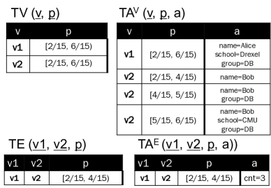
(a) $T1\cap^{T}T2$.

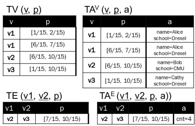
(b) $T1\setminus^{T}T2$.

Figure 17: Binary operators.

Appendix B Additional results.

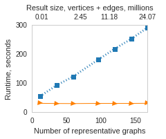
Figure 18: Slice on wiki-talk.

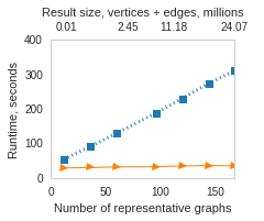
Figure 19: Map on wiki-talk.

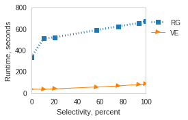
Figure 20: Subgraph on wiki-talk.

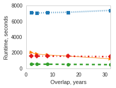
Figure 21: Union on nGrams.

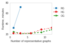
Figure 22: PageRank on Twitter.

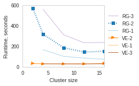
Figure 23: Scaling slice on wiki-talk.

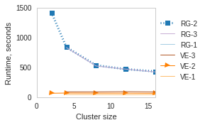
Figure 24: V-subgraph on wiki-talk.

Plots and discussion in this section complement experimental results presented in Section 6.

Figure 20 shows performance of VE and RG on slice over wiki-talk. It exhibits the same trend as on the nGrams dataset in Figure 9 but on a smaller scale.

Figure 20 shows performance of VE and RG on vertex subgraph over wiki-talk. Wiki-talk dataset is small enough that broadcast join can be used for constraining the edges, so the sudden worsening of performance is not observed, as it is in Figure 9.

We next examine how the different access methods scale with the size of the cluster. We varied the number of cluster workers while executing individual operations.

To examine the performance on slice, we fixed the slice interval size to be 4, 8, and 14 years (series -1, -2, and -3, respectively). As can be seen in Figure 23, the performance of VE did not change with the cluster size or the size of the interval. Our cluster stores the graph files on HDFS with no replication, and Spark does not currently support filter pushdown on dates (this is being addressed in one of the upcoming releases), so these results are expected as the operation is essentially just a file scan. RG performance did improve as the cluster grew, with the biggest reduction occurring by 8 slaves and diminishing returns thereafter.

Similar trends can be seen on vertex subgraph in Figure 24, where we fixed the query selectivity to be 20, 57, and 100%. There is no observable difference between different selectivity for RG, which is consistent with the subgraph experiment results.

We do not include results for every operation here as they all show the same trends – performance rapidly improves with increased cluster size up to a point and adding additional slaves is not beneficial thereafter.

References

- [1] C. R. Aberger, S. Tu, K. Olukotun, and C. Ré. Emptyheaded: A relational engine for graph processing. In Proceedings of the 2016 International Conference on Management of Data, SIGMOD Conference 2016, San Francisco, CA, USA, June 26 - July 01, 2016, pages 431–446, 2016.
- [2] C. C. Aggarwal and K. Subbian. Evolutionary network analysis. ACM Comput. Surv., 47(1):10:1–10:36, 2014.
- [3] S. Amer-Yahia, L. Lakshmanan, and C. Yu. SocialScope: Enabling information discovery on social content sites. In CIDR, 2009.
- [4] M. H. Böhlen. Temporal coalescing. In Encyclopedia of Database Systems, pages 2932–2936. 2009.
- [5] M. H. Böhlen et al. Coalescing in temporal databases. In VLDB, 1996.
- [6] M. H. Böhlen et al. Temporal compatibility. In Encyclopedia of Database Systems. 2009.
- [7] M. H. Böhlen, J. Gamper, and C. S. Jensen. How would you like to aggregate your temporal data? In TIME, 2006.
- [8] A. Casteigts, P. Flocchini, W. Quattrociocchi, and N. Santoro. Time-Varying Graphs and Dynamic Networks. In Proceedings of the 10th international conference on Ad-hoc, mobile, and wireless networks, volume 6811, pages 346–359, 2011.
- [9] J. Chan, J. Bailey, and C. Leckie. Discovering correlated spatio-temporal changes in evolving graphs. Knowledge and Information Systems, 16(1):53–96, 2008.
- [10] J. Chomicki. Temporal query languages: A survey. In Temporal Logic, First International Conference, ICTL ’94, Bonn, Germany, July 11-14, 1994, Proceedings, pages 506–534, 1994.
- [11] J. Chomicki and D. Toman. Temporal relational calculus. In Encyclopedia of Database Systems, pages 3015–3016. 2009.
- [12] A. Dignös, M. H. Böhlen, and J. Gamper. Temporal Alignment. In Proceedings of the 2012 international conference on Management of Data - SIGMOD ’12, pages 433–444, Scottsdale, Arizona, USA, 2012.
- [13] A. Ferreira. Building a reference combinatorial model for MANETs. IEEE Network, 18(5):24–29, 2004.
- [14] M. Gabielkov et al. Studying social networks at scale: Macroscopic anatomy of the twitter social graph. In SIGMETRICS, 2014.
- [15] B. George, J. M. Kang, and S. Shekhar. Spatio-Temporal Sensor Graphs (STSG): A Data Model for the Discovery of Spatio-Temporal Patterns. Intelligent Data Analysis, 13(3):457–475, 2009.
- [16] B. George and S. Shekhar. Time-aggregated graphs for modeling spatio-temporal networks. Journal on Data Semantics, 11:191–212, 2006.
- [17] J. Gonzalez, Y. Low, and H. Gu. Powergraph: Distributed graph-parallel computation on natural graphs. In OSDI, pages 17–30, 2012.
- [18] J. E. Gonzalez et al. GraphX: Graph processing in a distributed dataflow framework. In OSDI, 2014.
- [19] P.-y. Hsu and D. S. Parker. Improving SQL with Generalized Quantifiers. In ICDE, 1995.
- [20] W. Huo and V. J. Tsotras. Efficient Temporal Shortest Path Queries on Evolving Social Graphs. In Proceedings of the 26th International Conference on Scientific and Statistical Database Management, SSDBM ’14, pages 38:1–38:4, New York, NY, USA, 2014. ACM.
- [21] C. S. Jensen and R. T. Snodgrass. Temporal data models. In Encyclopedia of Database Systems, pages 2952–2957. 2009.
- [22] A. Kan, J. Chan, J. Bailey, and C. Leckie. A Query Based Approach for Mining Evolving Graphs. In Eighth Australasian Data Mining Conference (AusDM 2009), volume 101, Melbourne, Australia, 2009.
- [23] U. Khurana and A. Deshpande. Efficient Snapshot Retrieval over Historical Graph Data. In 2013 IEEE 29th International Conference on Data Engineering (ICDE), pages 997 – 1008, Brisbane, QLD, 2013.
- [24] U. Khurana and A. Deshpande. Storing and Analyzing Historical Graph Data at Scale. In Proceedings of the 19th International Conference on Extending Database Technology, EDBT’16, pages 65–76, Bordeaux, France, 2016.
- [25] K. G. Kulkarni and J. Michels. Temporal features in SQL: 2011. SIGMOD Record, 41(3):34–43, 2012.
- [26] A. G. Labouseur, J. Birnbaum, P. W. Olsen, S. R. Spillane, J. Vijayan, J. H. Hwang, and W. S. Han. The G* graph database: efficiently managing large distributed dynamic graphs. Distributed and Parallel Databases, 33(4):479–514, 2014.
- [27] K. Lerman, M. Rey, R. Ghosh, and J. H. Kang. Centrality Metric for Dynamic Networks. In Proceedings of the Eighth Workshop on Mining and Learning with Graphs, pages 70–77, Washington, D.C., 2010.
- [28] J. Li et al. Semantics and evaluation techniques for window aggregates in data streams. In ACM SIGMOD, 2005.
- [29] Y. Miao, W. Han, K. Li, M. Wu, F. Yang, L. Zhou, V. Prabhakaran, E. Chen, and W. Chen. ImmortalGraph: A System for Storage and Analysis of Temporal Graphs. ACM Transactions on Storage, 11(3):14–34, 2015.
- [30] C. Ren, E. Lo, B. Kao, X. Zhu, and R. Cheng. On Querying Historical Evolving Graph Sequences. Proceedings of the VLDB Endowment, 4(11):726–737, 2011.
- [31] I. Robinson, J. Webber, and E. Eifrem. Graph databases. O’Reilly Media, Inc., 2013.
- [32] K. Semertzidis, K. Lillis, and E. Pitoura. TimeReach: Historical Reachability Queries on Evolving Graphs. In Proceedings of the 18th International Conference on Extending Database Technology, pages 121–132, Brussels, Belgium, 2015.
- [33] W. Sun, A. Fokoue, K. Srinivas, A. Kementsietsidis, G. Hu, and G. T. Xie. Sqlgraph: An efficient relational-based property graph store. In Proceedings of the 2015 ACM SIGMOD International Conference on Management of Data, Melbourne, Victoria, Australia, May 31 - June 4, 2015, pages 1887–1901.
- [34] D. Toman. Point-stamped temporal models. In Encyclopedia of Database Systems, pages 2119–2123. 2009.
- [35] P. T. Wood. Query languages for graph databases. ACM SIGMOD Record, 41(1):50–60, mar 2012.
- [36] K. Xirogiannopoulos, U. Khurana, and A. Deshpande. Graphgen: Exploring interesting graphs in relational data. PVLDB, 8(12):2032–2035, 2015.
- [37] V. Zaychik Moffitt and J. Stoyanovich. Towards a distributed infrastructure for evolving graph analytics. In TempWeb, 2016.
- [38] E. Zimányi. Temporal aggregates and temporal universal quantification in standard SQL. SIGMOD Record, 35(2):16–21, 2006.