Spectral narrowing and spin echo for localized carriers with heavy-tailed Lévy distribution of hopping times

Abstract

We study analytically the free induction decay and the spin echo decay originating from the localized carriers moving between the sites which host random magnetic fields. Due to disorder in the site positions and energies, the on-site residence times, $\tau$, are widely spread according to the Lévy distribution. The power-law tail $\propto\tau^{-1-\alpha}$ in the distribution of $\tau$ does not affect the conventional spectral narrowing for $\alpha>2$, but leads to a dramatic acceleration of the free induction decay in the domain $2>\alpha>1$. The next abrupt acceleration of the decay takes place as $\alpha$ becomes smaller than $1$. In the latter domain the decay does not follow a simple-exponent law. To capture the behavior of the average spin in this domain, we solve the evolution equation for the average spin using the approach different from the conventional approach based on the Laplace transform. Unlike the free induction decay, the tail in the distribution of the residence times leads to the slow decay of the spin echo. The echo is dominated by realizations of the carrier motion for which the number of sites, visited by the carrier, is minimal.

I Introduction

A concept of the spectral narrowing of the magnetic resonance lineshape was quantified more than sixty years ago in a seminal paper Ref. Anderson, .

Figure 1: (Color online) The contrast between (a) Dyakonov-Perel spin relaxation with a single correlation time and (b) spin relaxation with broad distribution of the waiting times is illustrated schematically. Allowance for anomalously long waiting times accelerates the relaxation.

In application to free induction decay (FID), this concept can be recapped as follows. In the presence of the time-dependent random magnetic field, $b(t)$, the decay of the FID signal is determined by the average $\big{\langle}\exp\Big{[}i\int\limits_{0}^{t}dt^{\prime}b(t^{\prime})\Big{]}\big{\rangle}$. The character of the decay depends on the relation between the typical magnitude, $b_{\scriptscriptstyle 0}$, of $b(t)$ and the correlation time, $\tau$. For long correlation time $b_{\scriptscriptstyle 0}\tau\gg 1$, the decay is gaussian, $\propto\exp(-b_{\scriptscriptstyle 0}^{2}t^{2})$, reflecting the gaussian distribution of the magnitudes of $b(t)$. In the opposite limit, $b_{\scriptscriptstyle 0}\tau\ll 1$, the integrand rapidly changes sign, which is the origin of the spectral narrowing. If the time intervals between the subsequent sign changes are, $\delta t_{1}$, $\delta t_{2}$, $\delta t_{3}$, and so on, then the average, $\big{\langle}\exp\Big{[}i\int\limits_{0}^{t}dt^{\prime}b(t^{\prime})\Big{]}\big{\rangle}$, over the field realizations can be rewritten as $\exp\Big{[}-b_{\scriptscriptstyle 0}^{2}\sum\limits_{\scriptscriptstyle i=1}^{n}(\delta t_{i})^{2}\Big{]}$. On the other hand, the number of the sign changes, $n$, is determined by the condition $\sum\limits_{\scriptscriptstyle i=1}^{n}\delta t_{i}=t$. This leads to a simple exponential behavior, $\exp(-t/\tau_{\scriptscriptstyle s})$, of the FID signal, where

$$\frac{1}{\tau_{\scriptscriptstyle s}}=b_{\scriptscriptstyle 0}^{2}\frac{\overline{(\delta t)^{2}}}{\overline{\delta t}}.$$ (1)

If the random field is characterized by a single correlation time, $\tau_{\scriptscriptstyle 0}$, then the intervals $\delta t_{i}$ obey the Poisson distribution

$$p_{\scriptscriptstyle 0}(\delta t,\tau_{\scriptscriptstyle 0})=\frac{1}{\tau_{\scriptscriptstyle 0}}\exp\big{[}-\delta t/\tau_{\scriptscriptstyle 0}\big{]}.$$ (2)

Averaging with this distribution in Eq. (1) yields a well-known result, $\tau_{\scriptscriptstyle s}=1/2b_{\scriptscriptstyle 0}^{2}\tau_{\scriptscriptstyle 0}$, for the decay rate. In the field of semiconductors this result is also known as the Dyakonov-Perel spin relaxation timeDP1971 .

A nontrivial situation emerges when the correlation times, $\tau$, are broadly distributed. Then Eq. (1) takes the form

$$\frac{1}{\tau_{\scriptscriptstyle s}}=2b_{\scriptscriptstyle 0}^{2}\frac{\langle\tau^{2}\rangle}{\langle\tau\rangle},$$ (3)

where the averaging is performed over the distribution, $F(\tau)$, of the correlation times. Such a situation is generic, e.g., for the dispersive transport in disordered semiconductorsDT1 ; DT2 ; DT3 ; DT4 ; Harmon1 ; Harmon2 ; Baranovskii . Broad distribution of the $\tau$-values stems from the spread in the activation energies. Another example is a system with hopping transport, where the broad distribution of $\tau$ is the result of the spread in the hopping distances. In both cases $F(\tau)$ has a power-law tail: $F(\tau)\propto\tau^{-1-\alpha}$. Such a distribution, also known as the Lévy distribution, is normalizable for positive $\alpha$. However, for $\alpha<2$ the average $\langle\tau^{2}\rangle$ diverges. Formally, this implies that $\tau_{\scriptscriptstyle s}$ turns to zero. On the physical level, this means that, on certain occasions, the spin spends enough time in some given field to exercise a full rotation, see Fig. 1. Although the portion of these occasions is small $\sim\left(b_{\scriptscriptstyle 0}\tau_{\scriptscriptstyle 0}\right)^{\alpha}$, they change the average spin dynamics dramatically. Theoretical study of this dynamics is the subject of the present paper. We find that, for $\alpha<2$, the FID retains the form of a simple exponent, but the rate, $\tau_{\scriptscriptstyle s}^{-1}$, shortens and becomes a strong function of the tail parameter, $\alpha$. Our results can be summarized as

$$\frac{1}{\tau_{\scriptscriptstyle s}}=\begin{cases}D_{1}(\alpha)~{}b_{\scriptscriptstyle 0}^{2}\tau_{\scriptscriptstyle 0},~{}~{}~{}~{}~{}~{}~{}~{}~{}~{}\alpha>2\\ D_{2}(\alpha)~{}b_{\scriptscriptstyle 0}^{\alpha}\tau_{\scriptscriptstyle 0}^{\alpha-1},~{}~{}~{}~{}~{}2>\alpha>1\\ D_{3}(\alpha)~{}b_{\scriptscriptstyle 0},~{}~{}~{}~{}~{}~{}~{}~{}~{}~{}~{}~{}1>\alpha>0,\end{cases}$$ (4)

where $D_{1}(\alpha)$, $D_{2}(\alpha)$, and $D_{3}(\alpha)$ are the dimensionless functions of the tail parameter. Change of the behavior of $\tau_{s}$ at $\alpha=2$ is due to the formal divergence of $\langle\tau^{2}\rangle$, while the change at $\alpha=1$ is due to the formal divergence of $\langle\tau\rangle$, which enters into the denominator of Eq. (3). We also find that the crossovers at $\alpha=2$ and $\alpha=1$ take place within narrow intervals: $|\alpha-2|\sim 1/|\ln b_{\scriptscriptstyle 0}\tau_{\scriptscriptstyle 0}|$ and $|\alpha-1|\sim 1/|\ln b_{\scriptscriptstyle 0}\tau_{\scriptscriptstyle 0}|$.

Another phenomenon which is strongly affected in the presence of multiple waiting time is spin echoKlauderAnderson . The effect of the tail in $F(\tau)$ on the echo is opposite to the effect of $F(\tau)$ on the spin relaxation rate. The echo decays slower due to this tail. The average echo signal is determined by the realizations with longest waiting times.

The paper is organized as follows. In Sect. II we derive a closed equation for the FID averaged over the realizations of random fields. Asymptotic (in parameter $b_{\scriptscriptstyle 0}\tau_{\scriptscriptstyle 0}\ll 1$) solution of this equation is found in Sect. III, where we derive the result Eq. (4) and also find the crossover behaviors near $\alpha=2$ and $\alpha=1$. In Sect. IV we analyze the decay of the average echo signal. Concluding remarks are presented in Sect. V.

II Basic equation for average FID with multiple relaxation times

As it was mentioned in the Introduction, the physical picture which we have in mind is the carrier motion between the sites either by hopping or by trapping-detrapping processDT1 ; DT2 ; DT3 ; DT4 ; Harmon1 ; Harmon2 ; Baranovskii . The time-dependent magnetic field of a hyperfine originhyperfine , acting on the carrier spin, represents a sequence of steps ${\bm{b}}(t)=\sum_{i}{\bm{b}_{i}}\left[\Theta(t_{i+1}-t)-\Theta(t-t_{i})\right]$, where $\Theta(x)$ is the step-function and the step durations, $(t_{i+1}-t_{i})$, are distributed according to the Poisson distribution Eq. (2), in which $\tau_{\scriptscriptstyle 0}$ is distributed according to $F(\tau)$. Since the sites are separated in space, random fields, ${\bm{b}}_{i}$, at different sites are completely uncorrelated. We also assume that the motion is three-dimensional, so that the effect of occasional returns to the same siteCzech ; Robert1 ; Mkhitaryan are negligible.

Suppose that at time moment $t=0$ a carrier occupies the site $i=0$, and its spin is directed along the $z$-axis. After time $t$ the carrier can either remain on the site $i=1$ or hop on the neighboring site $i=1$. The probability to stay is $p_{\scriptscriptstyle 0}(t,\tau^{\scriptscriptstyle(0)})$, defined by Eq. (2), where $\tau^{\scriptscriptstyle(0)}$ is a waiting time for the hop $0\rightarrow 1$. We assume that the external magnetic field is directed along $x$-axis, so that only the $x$-components of the fields $b^{\scriptscriptstyle(0)}$ and $b^{\scriptscriptstyle(1)}$ on the sites $i=0$ and $i=1$ are important. If the carrier stays on $i=0$, then the $z$-projection of its spin after time $t$ is equal to $\cos b^{\scriptscriptstyle(0)}t$. If the carrier hops after time $t_{\scriptscriptstyle 1}<t$, then this projection is equal to $\cos\left[b^{\scriptscriptstyle(0)}t_{\scriptscriptstyle 1}+b^{\scriptscriptstyle(1)}(t-t_{\scriptscriptstyle 1})\right]$. Taking into account that the moments $t_{\scriptscriptstyle 1}$ are random, the value of $S_{z}(t)$ can be presented as a sum

$$S_{z}(t)= p_{\scriptscriptstyle 0}(t,\tau^{\scriptscriptstyle(0)})\cos b^{\scriptscriptstyle(0)}t$$ (5)

$$+\int\limits_{0}^{t}dt_{\scriptscriptstyle 1}\frac{d(1-p_{\scriptscriptstyle 0}(t_{\scriptscriptstyle 1},\tau^{\scriptscriptstyle(0)}))}{dt_{\scriptscriptstyle 1}}\cos\left[b^{\scriptscriptstyle(0)}t_{\scriptscriptstyle 1}+b^{\scriptscriptstyle(1)}(t-t_{\scriptscriptstyle 1})\right].$$

The derivative in the integrand is the probability density of the hop. If there is a site $i=2$ on which the carrier can hop from $i=1$, the expression Eq. (5) gets modified. It acquires a third term describing the possibility of the hop $1\rightarrow 2$, with corresponding waiting time $\tau^{\scriptscriptstyle(1)}$. If this hop takes place, $S_{z}$ acquires the value $\cos\left[b^{\scriptscriptstyle(0)}t_{\scriptscriptstyle 1}+b^{\scriptscriptstyle(1)}t_{\scriptscriptstyle 2}+b^{\scriptscriptstyle(2)}(t-t_{\scriptscriptstyle 1}-t_{\scriptscriptstyle 2})\right]$, where $t_{\scriptscriptstyle 2}$ is a random residence time on the site $i=1$ and $b^{\scriptscriptstyle(2)}$ is the random field on the site $i=2$.

For infinite number of possible hops Eq. (5) transforms into an infinite series. Averaging each term over the gaussian distribution of magnetic fields and realizations of waiting times generates a series for average spin projection, $\overline{S}_{z}(t)$. It can be verified that $\overline{S}_{z}(t)$ satisfies the equation

$$\overline{S}_{z}(t)=\Big{\langle}e^{-t/\tau}\Big{\rangle}e^{-b_{\scriptscriptstyle 0}^{2}t^{2}}+\int\limits_{0}^{t}dt_{1}A(t_{1})\overline{S}_{z}(t-t_{1}),$$ (6)

where the function $A(t)$ is defined as

$$A(t)=\Big{\langle}\frac{1}{\tau}e^{-t/\tau}\Big{\rangle}e^{-b_{\scriptscriptstyle 0}^{2}t^{2}},$$ (7)

and $\langle....\rangle$ stands for averaging over the broadly distributed waiting times. The above closed equation describes the averaged spin relaxation. In the next Section we solve it in different domains of the tail parameter $\alpha$.

III Solution of Equation for ${\overline{S}}_{z}(t)$

For concreteness, we choose the distribution function of the waiting times in the form

$$F(\tau)=\frac{C_{\alpha}\tau_{\scriptscriptstyle 0}^{\alpha}}{(\tau_{\scriptscriptstyle 0}^{2}+\tau^{2})^{\frac{1+\alpha}{2}}}.$$ (8)

For $\tau\gg\tau_{\scriptscriptstyle 0}$, we have $F(\tau)\propto\tau^{-1-\alpha}$, and the coefficient $C_{\alpha}$ which insures the normalization is given by

$$C_{\alpha}=\frac{2\Gamma(\frac{1+\alpha}{2})}{\pi^{1/2}\Gamma(\frac{\alpha}{2})}.$$ (9)

As we demonstrate in the Appendix, for the multiple trapping modelBaranovskii the form Eq. (8) describes accurately not only the tail but the entire body of the distribution. While the typical time, $\tau_{\scriptscriptstyle 0}$, is short, $\tau_{\scriptscriptstyle 0}\ll b_{\scriptscriptstyle 0}^{-1}$, the distribution has a long tail $F(\tau)\propto\tau^{-1-\alpha}$.

We start the analysis of the basic equation Eq. (6) by noticing that at times $t\gg\tau_{\scriptscriptstyle 0}$ the first term is small. Indeed, averaging with the help of Eq. (8), yields

$$\Big{\langle}e^{-t/\tau}\Big{\rangle}\sim\Big{(}\frac{\tau_{\scriptscriptstyle 0}}{t}\Big{)}^{\alpha}.$$ (10)

A crucial step of the analysis is making use of the fact that spin relaxation takes place over a large number of hops. This allows one to expand $\overline{S}_{z}$ in the integrand

$$\overline{S}_{z}(t-t_{1})\approx\overline{S}_{z}(t)-t_{1}\frac{d\overline{S}_{z}}{dt}(t).$$ (11)

Upon this expansion, Eq. (6) can be easily solved yielding

$$\overline{S}_{z}(t)=\exp\Big{[}-\int\limits_{0}^{t}dt_{1}\Phi(t_{1})\Big{]},$$ (12)

where the function $\Phi(t)$ is defined as

$$\Phi(t)=\frac{1-\int\limits_{0}^{t}dt_{2}A(t_{2})}{\int\limits_{0}^{t}dt_{2}t_{2}A(t_{2})}.$$ (13)

For $\alpha>1$ the characteristic time, $\tau_{s}$, for the spin dynamics is much longer than $b_{\scriptscriptstyle 0}^{-1}$ (we will check this assumption later). On the other hand, even for wide distribution of the waiting times, the function $A(t)$ falls off dramatically for $t\gtrsim b_{\scriptscriptstyle 0}^{-1}$. This allows one to extend the upper limits in the integrals in Eq. (13) to $\infty$. Then Eq. (12) reduces to a simple exponential decay

$$\overline{S}_{z}(t)=\exp\Big{(}-\frac{t}{\tau_{\scriptscriptstyle s}}\Big{)},$$ (14)

with the decay rate given by

$$\frac{1}{\tau_{\scriptscriptstyle s}}=\Phi(\infty)=\frac{\int\limits_{0}^{\infty}dt\Big{\langle}\frac{1}{\tau}e^{-t/\tau}\Big{\rangle}\Big{(}1-e^{-b_{\scriptscriptstyle 0}^{2}t^{2}}\Big{)}}{\int\limits_{0}^{\infty}dtt\Big{\langle}\frac{1}{\tau}e^{-t/\tau}\Big{\rangle}e^{-b_{\scriptscriptstyle 0}^{2}t^{2}}}.$$ (15)

If the averages in the numerator and denominator decayed rapidly at $t\gtrsim\tau_{\scriptscriptstyle 0}$, we would be allowed, by virtue of the condition $b_{\scriptscriptstyle 0}\tau_{\scriptscriptstyle 0}\ll 1$, to replace $\exp\big{(}-b_{\scriptscriptstyle 0}^{2}t^{2}\big{)}$ by $1$ in the denominator and expand $\Big{[}1-\exp\big{(}-b_{\scriptscriptstyle 0}^{2}t^{2}\big{)}\Big{]}$ in the numerator. In this way, we would retrieve the standard expression Eq. (3) for the Dyakonov-Perel relaxation time. Calculating $\langle\tau^{2}\rangle$ and $\langle\tau\rangle$ with the help of the distribution Eq. (8) we find

$$\frac{1}{\tau_{\scriptscriptstyle s}}=\frac{\pi^{1/2}(\alpha-1)\Gamma(\frac{\alpha-2}{2})}{2\Gamma(\frac{\alpha+1}{2})}b_{\scriptscriptstyle 0}^{2}\tau_{\scriptscriptstyle 0}$$ (16)

This expression is valid if $\langle\tau^{2}\rangle$ is finite, which corresponds to $\alpha>2$. The prefactor in this expression specifies the function $D_{1}(\alpha)$ in Eq. (4). The function $D_{1}(\alpha)$ falls off monotonically with $\alpha$. At $\alpha\gg 1$ it behaves as $\Big{(}\frac{2\pi}{\alpha}\Big{)}^{1/2}$.

In the domain $1<\alpha<2$ the value of $\langle\tau^{2}\rangle$ diverges while $\langle\tau\rangle$ remains finite. The latter still allows one to set $b_{\scriptscriptstyle 0}=0$ in the denominator of Eq. (15), but the numerator cannot be expanded anymore. The explicit expression for the numerator in Eq. (15) reads

$$\int\limits_{0}^{\infty}dt\Big{\langle}\frac{1}{\tau}e^{-t/\tau}\Big{\rangle}\Big{(}1-e^{-b_{\scriptscriptstyle 0}^{2}t^{2}}\Big{)}=$$ (17)

$$\int\limits_{0}^{\infty}d\tau\int\limits_{0}^{\infty}dt\frac{C_{\alpha}\tau_{\scriptscriptstyle 0}^{\alpha}}{(\tau_{\scriptscriptstyle 0}^{2}+\tau^{2})^{\frac{1+\alpha}{2}}\tau}e^{-t/\tau}\Big{(}1-e^{-b_{\scriptscriptstyle 0}^{2}t^{2}}\Big{)}$$

Upon introducing the new variables $z=t/\tau$ and $w=b_{\scriptscriptstyle 0}z\tau$, the integral in the right-hand side takes the form

$$C_{\alpha}(b_{\scriptscriptstyle 0}\tau_{\scriptscriptstyle 0})^{\alpha}\int\limits_{0}^{\infty}dz~{}z^{\alpha}e^{-z}\int\limits_{0}^{\infty}dw\frac{1-e^{-w^{2}}}{[(b_{\scriptscriptstyle 0}\tau_{\scriptscriptstyle 0}z)^{2}+w^{2}]^{\frac{\alpha+1}{2}}}.$$ (18)

Since the characteristic $z$ in Eq. (18) is $\sim 1$, we can neglect $(b_{\scriptscriptstyle 0}\tau_{\scriptscriptstyle 0}z)^{2}$ in the denominator, after which the double integral factorizes, yielding

$$C_{\alpha}(b_{\scriptscriptstyle 0}\tau_{\scriptscriptstyle 0})^{\alpha}\Gamma(\alpha)\Gamma\Big{(}\frac{2-\alpha}{2}\Big{)}.$$ (19)

Then the corresponding expression for the relaxation time in the domain $1<\alpha<2$ acquires the form

$$\frac{1}{\tau_{\scriptscriptstyle s}}=(\alpha-1)\Gamma(\alpha)\Gamma\Big{(}\frac{2-\alpha}{2}\Big{)}\frac{(b_{\scriptscriptstyle 0}\tau_{\scriptscriptstyle 0})^{\alpha}}{\tau_{\scriptscriptstyle 0}},$$ (20)

where the prefactor specifies the function $D_{2}(\alpha)$ in Eq. (4).

III.1 Vicinity of $\alpha=2$

We see that at the demarkation value $\alpha=2$ both functions $D_{1}(\alpha)$ and $D_{2}(\alpha)$ diverge, so that the expressions Eq. (16) and Eq. (20) yield $\tau_{\scriptscriptstyle s}\rightarrow 0$. This suggests that the crossover domain should be treated more carefully. Namely, we rewrite the integral over $w$ in Eq. (18) as

$$\int\limits_{0}^{\infty}dw\frac{1-e^{-w^{2}}}{[(b_{\scriptscriptstyle 0}\tau_{\scriptscriptstyle 0}z)^{2}+w^{2}]^{\frac{\alpha+1}{2}}}=\frac{\Gamma(\frac{2-\alpha}{2})}{\alpha}$$ (21)

$$+\int\limits_{0}^{\infty}dw\Big{[}\frac{1}{[(b_{\scriptscriptstyle 0}\tau_{\scriptscriptstyle 0}z)^{2}+w^{2}]^{\frac{\alpha+1}{2}}}-\frac{1}{w^{\alpha+1}}\Big{]}\Big{(}1-e^{-w^{2}}\Big{)}.$$

The integral in the right-hand side converges at small $w\sim b_{\scriptscriptstyle 0}\tau_{\scriptscriptstyle 0}z$, which allows one to expand $(1-e^{-w^{2}})$. Upon introducing the variable $v=(\frac{w}{b_{\scriptscriptstyle 0}\tau_{\scriptscriptstyle 0}z})^{2}$, this integral takes the form

$$\frac{(b_{\scriptscriptstyle 0}\tau_{\scriptscriptstyle 0}z)^{2-\alpha}}{2}\int\limits_{0}^{\infty}dv\Big{[}\frac{v^{1/2}}{(1+v)^{\frac{\alpha+1}{2}}}-\frac{1}{v^{\frac{\alpha}{2}}}\Big{]}.$$ (22)

Now we rewrite the integral $\int\limits_{0}^{\infty}\frac{dv}{v^{\frac{\alpha}{2}}}$ as a sum of integrals from $0$ to $1$ and from $1$ to $\infty$. The integral from $1$ to $\infty$ is then combined with the first integral in Eq. (22) in which domain of integration is shifted by $1$. This yields

$$\frac{(b_{\scriptscriptstyle 0}\tau_{\scriptscriptstyle 0}z)^{2-\alpha}}{2}\Big{[}-\int\limits_{0}^{1}dv\frac{1}{v^{\frac{\alpha}{2}}}+\int\limits_{1}^{\infty}dq\frac{(q+1)^{1/2}-q^{1/2}}{q^{\frac{\alpha+1}{2}}}\Big{]}.$$ (23)

Note that the second integral in the square brackets remains finite at $\alpha=2$, while the first integral diverges. Keeping only the diverging part and combining it with $\frac{1}{\alpha}\Gamma\Big{(}\frac{2-\alpha}{2}\Big{)}\approx\frac{1}{2-\alpha}$, we establish the behavior of the spin relaxation rate Eq. (20) near $\alpha=2$

$$\frac{1}{\tau_{\scriptscriptstyle s}}=2b_{\scriptscriptstyle 0}^{2}\tau_{\scriptscriptstyle 0}|\ln b_{\scriptscriptstyle 0}\tau_{\scriptscriptstyle 0}|\Upsilon\Big{(}(\alpha-2)|\ln b_{\scriptscriptstyle 0}\tau_{\scriptscriptstyle 0}|\Big{)}.$$ (24)

where the crossover function $\Upsilon(z)$ is defined as

$$\Upsilon(z)=\frac{1-e^{-z}}{z}.$$ (25)

Thus the expressions Eq. (16) and Eq. (20) are valid outside the interval $|\alpha-2|\sim|\ln b_{\scriptscriptstyle 0}\tau_{\scriptscriptstyle 0}|^{-1}$, which is parametrically narrow.

III.2 Vicinity of $\alpha=1$

We see that Eq. (20) yields $\tau_{\scriptscriptstyle s}\rightarrow\infty$ as $\alpha$ approaches $1$ from the above. This is the result of the divergence of $\langle\tau\rangle$ in this limit. To regularize the behavior of Eq. (20), we need to calculate the denominator in Eq. (15) more accurately. We start from the explicit form of this denominator

$$\int\limits_{0}^{\infty}dttA(t)=\int\limits_{0}^{\infty}d\tau\int\limits_{0}^{\infty}dt\frac{C_{\alpha}\tau_{\scriptscriptstyle 0}^{\alpha}}{(\tau_{\scriptscriptstyle 0}^{2}+\tau^{2})^{\frac{1+\alpha}{2}}\tau}te^{-t/\tau}e^{-b_{\scriptscriptstyle 0}^{2}t^{2}}$$ (26)

The same change of variables $z=t/\tau$ and $w=b_{\scriptscriptstyle 0}z\tau$, allows to cast the integral in the the form

$$C_{\alpha}\tau_{\scriptscriptstyle 0}(b_{\scriptscriptstyle 0}\tau_{\scriptscriptstyle 0})^{\alpha-1}\int\limits_{0}^{\infty}dz~{}z^{\alpha}e^{-z}\int\limits_{0}^{\infty}dw\frac{we^{-w^{2}}}{[(b_{\scriptscriptstyle 0}\tau_{\scriptscriptstyle 0}z)^{2}+w^{2}]^{\frac{\alpha+1}{2}}}.$$ (27)

Formally, the singular behavior of this integral at $\alpha=1$ follows from the fact that at $\alpha=1$ integration over $w$ yields logarithm if we neglect a small parameter $(b_{\scriptscriptstyle 0}\tau_{\scriptscriptstyle 0})^{2}$ in the denominator. To capture this behavior, we rewrite the integral over $w$ using the integration by parts

$$\int\limits_{0}^{\infty}dw\frac{we^{-w^{2}}}{[(b_{\scriptscriptstyle 0}\tau_{\scriptscriptstyle 0}z)^{2}+w^{2}]^{\frac{\alpha+1}{2}}}=$$ (28)

$$\frac{1}{\alpha-1}\Big{[}(b_{\scriptscriptstyle 0}\tau_{\scriptscriptstyle 0}z)^{1-\alpha}-\int\limits_{0}^{\infty}dw\frac{2we^{-w^{2}}}{[(b_{\scriptscriptstyle 0}\tau_{\scriptscriptstyle 0}z)^{2}+w^{2}]^{\frac{\alpha-1}{2}}}\Big{]}.$$

Now we can safely neglect $(b_{\scriptscriptstyle 0}\tau_{\scriptscriptstyle 0})^{2}$ in the denominator and perform the integration over $z$, which yields

$$\frac{C_{\alpha}\tau_{\scriptscriptstyle 0}(b_{\scriptscriptstyle 0}\tau_{\scriptscriptstyle 0})^{\alpha-1}}{\alpha-1}\Big{[}\Gamma(2\alpha-1)(b_{\scriptscriptstyle 0}\tau_{\scriptscriptstyle 0})^{1-\alpha}-\Gamma(\alpha)\Gamma(\frac{3-\alpha}{2})\Big{]}.$$ (29)

Finally, the behavior of $\tau_{\scriptscriptstyle s}$ in the vicinity of $\alpha=1$ can be expressed in terms of the crossover function $\Upsilon(z)$ defined by Eq. (25)

$$\frac{1}{\tau_{\scriptscriptstyle s}} =\frac{(\alpha-1)\Gamma(\alpha)\Gamma\Big{(}\frac{2-\alpha}{2}\Big{)}}{\Gamma(2\alpha-1)-\Gamma(\alpha)\Gamma(\frac{3-\alpha}{2})(b_{\scriptscriptstyle 0}\tau_{\scriptscriptstyle 0})^{\alpha-1}}\frac{(b_{\scriptscriptstyle 0}\tau_{\scriptscriptstyle 0})^{\alpha}}{\tau_{\scriptscriptstyle 0}}$$ (30)

$$\approx\frac{(\alpha-1)\pi^{1/2}}{1-(b_{\scriptscriptstyle 0}\tau_{\scriptscriptstyle 0})^{\alpha-1}}\frac{(b_{\scriptscriptstyle 0}\tau_{\scriptscriptstyle 0})^{\alpha}}{\tau_{\scriptscriptstyle 0}}=\frac{\pi^{1/2}b_{\scriptscriptstyle 0}}{|\ln b_{\scriptscriptstyle 0}\tau_{\scriptscriptstyle 0}|}\frac{1}{\Upsilon\Big{(}(1-\alpha)|\ln b_{\scriptscriptstyle 0}\tau_{\scriptscriptstyle 0}|\Big{)}}.$$

Unlike Eq. (24), the crossover function appears in the denominator. Directly at $\alpha=1$ Eq. (30) yields

$$\frac{1}{\tau_{\scriptscriptstyle s}}=\pi^{1/2}\frac{b_{\scriptscriptstyle 0}}{|\ln b_{\scriptscriptstyle 0}\tau_{\scriptscriptstyle 0}|}.$$ (31)

The fact that for all $\alpha$ greater or equal $1$ the value $\tau_{\scriptscriptstyle s}^{-1}$ is smaller than $b_{\scriptscriptstyle 0}$ justifies the ansatz: $\overline{S}_{z}(t-t_{1})=\overline{S}_{z}(t)-t_{1}d\overline{S}_{z}/dt$ and the extension of the upper limit in Eq. (13) to $\infty$.

Figure 2: (Color online) (a) Acceleration of the relaxation rate with decreasing the tail-parameter, $\alpha$, is illustrated in the domain $0.6<\alpha<1.5$. Dashed red curves are plotted from Eq. (38) (for $\alpha<1$), and Eq. (20) (for $1<\alpha<1.5$). The curves exhibit a dip near $\alpha=1$. They are connected by the crossover expression Eq. (30). (b) Domain $1<\alpha<3$. Dashed red curves are plotted from Eq. (20) (for $1<\alpha<2$), and from Eq. (16) (for $\alpha>2$). The curves exhibit a divergence near $\alpha=2$. They are connected by the crossover expression Eq. (24). All the curves are plotted for $b_{\scriptscriptstyle 0}\tau_{\scriptscriptstyle 0}=10^{-3}$.

III.3 $\alpha<1$

For $\alpha<1$ we cannot extend the limits of integration in Eq. (13) to infinity. Instead, we rewrite the expression Eq. (7) for $A(t)$ as follows

$$A(t)=\Big{\langle}\frac{1}{\tau}e^{-t/\tau}\Big{\rangle}\Big{(}e^{-b_{\scriptscriptstyle 0}^{2}t^{2}}-1\Big{)}+\Big{\langle}\frac{1}{\tau}e^{-t/\tau}\Big{\rangle}.$$ (32)

The integration over $t$ in the second term can be carried out explicitly. Then Eq. (13) acquires the form

$$\Phi(t)=\frac{\Big{\langle}e^{-t/\tau}\Big{\rangle}+\int\limits_{0}^{t}dt_{2}\Big{\langle}\frac{1}{\tau}e^{-t_{2}/\tau}\Big{\rangle}\Big{(}1-e^{-b_{\scriptscriptstyle 0}^{2}t_{2}^{2}}\Big{)}}{\int\limits_{0}^{t}dt_{2}t_{2}\Big{\langle}\frac{1}{\tau}e^{-t_{2}/\tau}\Big{\rangle}e^{-b_{\scriptscriptstyle 0}^{2}t_{2}^{2}}}.$$ (33)

In calculating both averages we can use the power-law tail of the distribution Eq. (8)

$$\Big{\langle}\frac{1}{\tau}e^{-t/\tau}\Big{\rangle}\approx C_{\alpha}\frac{\tau_{\scriptscriptstyle 0}^{\alpha}}{t^{\alpha+1}}\Gamma(\alpha+1),~{}~{}\Big{\langle}e^{-t/\tau}\Big{\rangle}\approx C_{\alpha}\frac{\tau_{\scriptscriptstyle 0}^{\alpha}}{t^{\alpha}}\Gamma(\alpha).$$ (34)

This expressions apply for $t\gg\tau_{\scriptscriptstyle 0}$. Substituting them into Eq. (33) and then Eq. (34) into Eq. (12), we arrive at the final result for $\overline{S}_{z}(t)$

$$\overline{S}_{z}(t)=\exp\Bigg{[}-\int\limits_{b_{\scriptscriptstyle 0}\tau_{\scriptscriptstyle 0}}^{b_{\scriptscriptstyle 0}t}dx\frac{\frac{1}{x^{\alpha}}+\alpha\int\limits_{0}^{x}dx_{1}x_{1}^{-\alpha-1}(1-e^{-x_{1}^{2}})}{\alpha\int\limits_{0}^{x}dx_{1}x_{1}^{-\alpha}e^{-x_{1}^{2}}}\Bigg{]}.$$ (35)

To analyze Eq. (35) in the domain $\tau_{\scriptscriptstyle 0}<t<b_{\scriptscriptstyle 0}^{-1}$, we note that for small $x$ the integrand in the exponent behaves as $\frac{1-\alpha}{\alpha x}$ which leads to the power-law decay of $\overline{S}_{z}(t)$

$$\overline{S}_{z}(t)\Big{|}_{t\ll b_{\scriptscriptstyle 0}^{-1}}\approx\exp\Big{[}-\frac{1-\alpha}{\alpha}\ln(t/\tau_{\scriptscriptstyle 0})\Big{]}=\Big{(}\frac{\tau_{\scriptscriptstyle 0}}{t}\Big{)}^{\frac{1-\alpha}{\alpha}}.$$ (36)

This behavior should be compared to the first term in Eq. (6), which we neglected. The power-law Eq. (36) dominates at $\alpha>0.6$.

In the long-time limit $b_{\scriptscriptstyle 0}t\gg 1$ the integral in Eq. (35) is determined by large $x$. For large $x$ the integrand saturates at the value $\frac{(1-\alpha)\Gamma(\frac{2-\alpha}{2})}{\alpha\Gamma(\frac{3-\alpha}{2})}$, so that the resulting expression for $\overline{S}_{z}(t)$ reads

$$\overline{S}_{z}(t)\Big{|}_{t\gg b_{\scriptscriptstyle 0}^{-1}}\approx\Big{(}b_{\scriptscriptstyle 0}\tau_{\scriptscriptstyle 0}\Big{)}^{\frac{1-\alpha}{\alpha}}\exp\Big{[}-\frac{(1-\alpha)\Gamma(\frac{2-\alpha}{2})}{\alpha\Gamma(\frac{3-\alpha}{2})}b_{\scriptscriptstyle 0}t\Big{]}.$$ (37)

Since we neglected the first term in Eq. (6), the result Eq. (37) does not capture the initial stage of the decay, which is dominated by this first term. The decay in the entire time domain is described by Eq. (37) when $\alpha$ is so close to $1$ that the prefactor in Eq. (37) is not small. Then Eq. (37) captures the spin decay which is a simple exponent with

$$\frac{1}{\tau_{\scriptscriptstyle s}}\approx(1-\alpha)\pi^{1/2}b_{\scriptscriptstyle 0}.$$ (38)

Comparing to Eq. (4), we conclude that the function $D_{3}(\alpha)$ has the form $(1-\alpha)\pi^{1/2}$ near $\alpha=1$. Note, that this expression is consistent with Eq. (30) for $(\alpha-1)\gg|\ln(b_{\scriptscriptstyle 0}\tau_{\scriptscriptstyle 0})|^{-1}$ .

The overall behavior of the relaxation rate with $\alpha$ is illustrated in Fig. 2. In Fig. 3 we plot the time evolution of $\ln\overline{S}_{z}(t)$ using the general expression Eq. (35). We see that, the smaller is $\alpha$, the later the curves converge to the straight lines corresponding to a simple exponential behavior. The convergence is final only for biggest $\alpha=0.9$. For smaller $\alpha$-values the slopes keep increasing with time beyond the maximal $t=1.5/b_{\scriptscriptstyle 0}$ shown in the figure. The slopes saturate at the values predicted by Eq. (37) only at very large times.

Figure 3: (Color online) The time evolution of $|\ln\overline{S}_{z}(t)|$ is plotted from Eq. (35) for $b_{\scriptscriptstyle 0}\tau_{\scriptscriptstyle 0}=10^{-3}$ and the values of the tail-parameter: $\alpha=0.9$ (green), $\alpha=0.7$ (purple), and $\alpha=0.5$ (black). The smaller is $\alpha$, the later the curves converge to the straight lines. The convergence is final only for $\alpha=0.9$. For smaller $\alpha$ the slopes keep increasing with time beyond the maximal $t=1.5/b_{\scriptscriptstyle 0}$ and saturate at the values predicted by Eq. (37) only at very large times. The domain where the first term in Eq. (6) dominates the decay corresponds to $b_{\scriptscriptstyle 0}t\lesssim 10^{-3}$, and is not represented in the figure.

IV Spin echo decay with a Lévy-type waiting times distribution

It is well knownKlauderAnderson that the motion narrowing strongly affects the decay of the spin echo, which is formally defined as ${\overline{S}}_{E}(T)=\big{\langle}\exp\Big{[}i\Big{(}\int\limits_{0}^{\frac{T}{2}}dtb(t)-\int\limits_{\frac{T}{2}}^{T}dtb(t)\Big{)}\Big{]}\big{\rangle}$. If the random magnetic field is characterized by a single correlation time $\tau$, the decay of the spin echo would follow the FID signal, i.e. ${\overline{S}}_{E}(T)={\overline{S}}(T)$. The situation is very different for the broad distribution of $\tau$. Indeed, the shortening of the FID time, $\tau_{\scriptscriptstyle s}$, for distribution Eq. (8) with power-law tail was due to the possibility for a carrier to occasionally sit on a given site, $i$, during the time, $\tau_{\scriptscriptstyle i}$, much longer than a typical time, $\tau_{\scriptscriptstyle 0}$. These sites give anomalously strong contribution, $\big{\langle}\exp\Big{[}i\int\limits_{t_{\scriptscriptstyle i}}^{t_{\scriptscriptstyle i}+\tau_{\scriptscriptstyle i}}dtb_{\scriptscriptstyle i}(t)\Big{]}\big{\rangle}$, to the decay. The same physics suggests that, for distribution of $\tau$ with power-law tail, the echo signal will decay slowly with $T$. This is because the contributions from anomalously long residence times are eliminated in the echo signal. To quantify this statement, consider a situation when a carrier populates a certain site, $i$, at time $T_{\scriptscriptstyle 1}<T/2$ and leaves it at time $T_{\scriptscriptstyle 2}>T/2$. Then the contribution from this site to the unaveraged echo signal is given by

$$\exp\Big{\{}ib_{\scriptscriptstyle i}\Big{[}\Big{(}\frac{T}{2}-T_{\scriptscriptstyle 1}\Big{)}-\Big{(}T_{\scriptscriptstyle 2}-\frac{T}{2}\Big{)}\Big{]}\Big{\}}=\exp\Big{[}ib_{\scriptscriptstyle i}\Big{(}T-T_{\scriptscriptstyle 1}-T_{\scriptscriptstyle 2}\Big{)}\Big{]}.$$ (39)

Assume now, that the carrier makes many hops before arrival to the site $i$ and many hops after departure from the site $i$. Then the probabilities to preserve spin during the time intervals $(0,T_{\scriptscriptstyle 1})$ and $(T_{\scriptscriptstyle 2},T)$ are given by     $\exp\big{[}-T{\scriptscriptstyle 1}/\tau_{\scriptscriptstyle s}\big{]}$ and $\exp\big{[}-\left(T-T{\scriptscriptstyle 2}\right)/\tau_{\scriptscriptstyle s}\big{]}$, respectively. As a result, the contribution to ${\overline{S}}_{E}(T)$ from this realization of the random fields reads

$$\int\limits_{0}^{\frac{T}{2}}\frac{dT_{\scriptscriptstyle 1}e^{-\frac{T_{\scriptscriptstyle 1}}{\tau_{\scriptscriptstyle s}}}}{\tau_{\scriptscriptstyle s}}\int\limits_{\frac{T}{2}}^{T}\frac{dT_{\scriptscriptstyle 2}e^{-\frac{T-T_{\scriptscriptstyle 2}}{\tau_{\scriptscriptstyle s}}}}{\tau_{\scriptscriptstyle s}}\Big{\langle}p_{\scriptscriptstyle 0}(T_{\scriptscriptstyle 2}-T_{\scriptscriptstyle 1},\tau)\Big{\rangle}e^{-b_{\scriptscriptstyle 0}^{2}(T-T_{\scriptscriptstyle 1}-T_{\scriptscriptstyle 2})^{2}}.$$ (40)

To analyze this expression, it is convenient to introduce a new variable, $T_{\scriptscriptstyle 3}=T-T_{\scriptscriptstyle 2}$. Then it takes the form

$$\int\limits_{0}^{\frac{T}{2}}\frac{dT_{\scriptscriptstyle 1}e^{-\frac{T_{\scriptscriptstyle 1}}{\tau_{\scriptscriptstyle s}}}}{\tau_{\scriptscriptstyle s}}\int\limits_{0}^{\frac{T}{2}}\frac{dT_{\scriptscriptstyle 3}e^{-\frac{T_{\scriptscriptstyle 3}}{\tau_{\scriptscriptstyle s}}}}{\tau_{\scriptscriptstyle s}}\Big{\langle}p_{\scriptscriptstyle 0}(T-T_{\scriptscriptstyle 3}-T_{\scriptscriptstyle 1},\tau)\Big{\rangle}e^{-b_{\scriptscriptstyle 0}^{2}(T_{\scriptscriptstyle 3}-T_{\scriptscriptstyle 1})^{2}}.$$ (41)

The average in Eq. (41) is equal to $C_{\alpha}\Gamma(\alpha)\tau_{\scriptscriptstyle 0}^{\alpha}/\big{(}T-T_{\scriptscriptstyle 3}-T_{\scriptscriptstyle 1}\big{)}^{\alpha}$, see Eq. (34).

The most sound consequence of Eq. (41) is that the echo signal survives at times much longer than $\tau_{\scriptscriptstyle s}$. Indeed, characteristics $T_{\scriptscriptstyle 1}$, $T_{\scriptscriptstyle 3}$ in Eq. (41) are $\sim\tau_{\scriptscriptstyle s}$. For $T\gg\tau_{\scriptscriptstyle s}$ the upper limits in the integrals can be extended to infinity, while the average can be replaced by $C_{\alpha}\Gamma(\alpha)\tau_{\scriptscriptstyle 0}^{\alpha}/T^{\alpha}$. Then we get

$$C_{\alpha}\Gamma(\alpha)\Big{(}\frac{\tau_{\scriptscriptstyle 0}}{T}\Big{)}^{\alpha}\int\limits_{0}^{\infty}dx~{}e^{-x}\int\limits_{0}^{\infty}dy~{}e^{-y}\exp\Big{[}-b_{\scriptscriptstyle 0}^{2}\tau_{\scriptscriptstyle s}^{2}(x-y)^{2}\Big{]},$$ (42)

where we have introduces the dimensionless variables $x=T_{\scriptscriptstyle 1}/\tau_{\scriptscriptstyle s}$ and $y=T_{\scriptscriptstyle 3}/\tau_{\scriptscriptstyle s}$. Within a numerical constant the double integral is equal to $\big{(}b_{\scriptscriptstyle 0}\tau_{\scriptscriptstyle s}\big{)}^{-1}$. Thus, we conclude that the echo signal falls off as a power law:

$${\overline{S}}_{E}(T)\sim\big{(}b_{\scriptscriptstyle 0}\tau_{\scriptscriptstyle s}\big{)}^{-1}\Big{(}\frac{\tau_{\scriptscriptstyle 0}}{T}\Big{)}^{\alpha}.$$ (43)

It is seen from Eq. (43) that ${\overline{S}}_{E}(T)$ contains a small parameter $\big{(}b_{\scriptscriptstyle 0}\tau_{\scriptscriptstyle s}\big{)}^{-1}$. At this point, we note that due to a long tail in the waiting time distribution, there is a non-exponential probability that during time, $T$, the carrier does not hop at all. The contribution to echo signal from such realizations does not contain random magnetic field and falls with $T$ in the same way as Eq. (43). Thus, the final result for the echo signal reads

$${\overline{S}}_{E}(T)=\Big{\langle}p_{\scriptscriptstyle 0}(T,\tau)\Big{\rangle}=C_{\alpha}\Gamma(\alpha)\Big{(}\frac{\tau_{\scriptscriptstyle 0}}{T}\Big{)}^{\alpha}.$$ (44)

V Concluding remarks

1. As a quantitative measure of acceleration of the relaxation rate, caused by the tail in the distribution, $F(\tau)$, one can consider a ratio of the times for the values of the tail-parameter $\alpha=1$ and $\alpha=2$. From Eqs. (24) and (31) one finds

$$\frac{\tau_{\scriptscriptstyle s}(\alpha=2)}{\tau_{\scriptscriptstyle s}(\alpha=1)}=\frac{\pi^{1/2}}{2b_{\scriptscriptstyle 0}\tau_{\scriptscriptstyle 0}|\ln(b_{\scriptscriptstyle 0}\tau_{\scriptscriptstyle 0})|^{2}}.$$ (45)

Both values of $\tau_{\scriptscriptstyle s}$ are determined by the tail. Parametrical, in $b_{\scriptscriptstyle 0}\tau_{\scriptscriptstyle 0}\ll 1$, difference between the two values is due to the fact that for $\alpha=1$ the portion of sites on which the carrier spin exercises a full rotation is $\sim(b_{\scriptscriptstyle 0}\tau_{\scriptscriptstyle 0})$ for $\alpha=1$ and $\sim(b_{\scriptscriptstyle 0}\tau_{\scriptscriptstyle 0})^{2}$ for $\alpha=2$.

2. In replacing the expression Eq. (12) by $\exp(-t/\tau_{\scriptscriptstyle s})$, we argued that this replacement is valid for $t\gtrsim b_{\scriptscriptstyle 0}^{-1}$. This means that in Eq. (12) we chose the lower limit $t_{1}\sim b_{\scriptscriptstyle 0}^{-1}$. Uncertainty in this lower limit leads to uncertainty in the prefactor in Eq. (14) $\sim\exp\Big{(}1/b_{\scriptscriptstyle 0}\tau_{\scriptscriptstyle s}\Big{)}$, which can be neglected since the product $b_{\scriptscriptstyle 0}\tau_{\scriptscriptstyle s}$ is big. Yet another contribution to the prefactor comes from $\int\limits_{\tau_{\scriptscriptstyle 0}}^{1/b_{\scriptscriptstyle 0}}dt_{1}\Phi(t_{\scriptscriptstyle 1})$. To estimate this contribution, we note that for $t\lesssim b_{\scriptscriptstyle 0}^{-1}$

$$\Phi(t)\Big{|}_{t<b_{\scriptscriptstyle 0}^{-1}}\approx\frac{1-\int\limits_{0}^{t}dt_{2}\Big{\langle}\frac{1}{\tau}e^{-t_{2}/\tau}\Big{\rangle}}{\int\limits_{0}^{t}dt_{2}t_{2}\Big{\langle}\frac{1}{\tau}e^{-t_{2}/\tau}\Big{\rangle}}=\frac{\Big{\langle}e^{-t/\tau}\Big{\rangle}}{\Big{\langle}\tau-(t+\tau)e^{-t/\tau}\Big{\rangle}}.$$ (46)

For $t\gtrsim\tau_{\scriptscriptstyle 0}$ we can neglect the second term in the denominator and perform integration over time, yielding

$$\int\limits_{0}^{t}dt_{1}\Phi(t_{1})\Big{|}_{t<b_{\scriptscriptstyle 0}^{-1}}=\frac{\Big{\langle}\tau(1-e^{-t/\tau})\Big{\rangle}}{\langle\tau\rangle}.$$ (47)

Thus, the contribution to the prefactor from small times does not exceed $1$. In fact, the contribution Eq. (47) comes from neglecting the first term, $\big{\langle}\exp(-\frac{t}{\tau}-b_{\scriptscriptstyle 0}^{2}t^{2})\big{\rangle}$, in the basic equation Eq. (6). We effectively replaced the first by the initial condition: $\overline{S}_{z}(t\sim\tau_{\scriptscriptstyle 0})=1$. More accurate calculation, based on the Laplace transform, suggests that for $\alpha>1$ the true prefactor is $1$.

3. Formal solution of Eq. (6) can be expressed in the form of the inverse Laplace transform, see e.g. Ref. Laplace,

$${\overline{S}}_{z}(t)=\frac{1}{2\pi i}\int\limits_{\gamma-i\infty}^{\gamma+i\infty}\frac{S_{z}^{\scriptscriptstyle(0)}(s)}{1-K(s)}$$ (48)

where the functions $S_{z}^{\scriptscriptstyle(0)}(s)$ and $K(s)$ are defined as

$$S_{z}^{\scriptscriptstyle(0)}(s) =\int\limits_{0}^{\infty}dt\Big{\langle}e^{-t/\tau}\Big{\rangle}e^{-st-b_{\scriptscriptstyle 0}^{2}t^{2}},$$ (49)

$$K(s) =\int\limits_{0}^{\infty}dt\Big{\langle}\frac{1}{\tau}e^{-t/\tau}\Big{\rangle}e^{-st-b_{\scriptscriptstyle 0}^{2}t^{2}}$$

The decay of ${\overline{S}}_{z}(t)$ is defined by the poles, $s=s_{\scriptscriptstyle 0}$, for which $K(s_{\scriptscriptstyle 0})=1$. For $\alpha>1$, one can retain only the smallest $s_{\scriptscriptstyle 0}$ and find it by expanding $K(s)$ at small $s$. This readily yields $s_{\scriptscriptstyle 0}=-\Phi(\infty)=-\tau_{\scriptscriptstyle s}^{-1}$, i.e. the same expression Eq. (15) for the decay rate as was found in Sect. II from the different approach. The justification for expanding $K(s)$ is that the exponent $\exp\big{(}-b_{\scriptscriptstyle 0}^{2}t^{2}\big{)}$ ensures the convergence of the integral Eq. (49) at $t\sim b_{\scriptscriptstyle 0}^{-1}$ when $\exp\big{(}-s_{\scriptscriptstyle 0}t\big{)}$ is close to $1$. Thus, for $\alpha>1$, the results of the two approaches to solving Eq. (6) coincide. Moreover, the solution Eq. (48) takes into account the first term in Eq. (6), which we have neglected. The prefactor in front of $\exp\big{(}-t/\tau_{\scriptscriptstyle s}\big{)}$ calculated from Eq. (48) is given by

$$-\frac{S_{z}^{\scriptscriptstyle(0)}(s_{\scriptscriptstyle 0})}{K^{\prime}(s_{\scriptscriptstyle 0})}\approx\frac{\int\limits_{0}^{\infty}dt\Big{\langle}e^{-t/\tau}\Big{\rangle}e^{-b_{\scriptscriptstyle 0}^{2}t^{2}}}{\int\limits_{0}^{\infty}dt~{}t\Big{\langle}\frac{1}{\tau}e^{-t/\tau}\Big{\rangle}e^{-b_{\scriptscriptstyle 0}^{2}t^{2}}}.$$ (50)

It appears that we can neglect the exponent $\exp\big{(}-b_{\scriptscriptstyle 0}^{2}t^{2}\big{)}$ in the integrands in the numerator and the denominator. This is because both integrals converge for $\alpha>1$ and are equal to $\langle\tau\rangle$, which is finite for $\alpha>1$. Thus the true prefactor is equal to $1$, as was mentioned above.

4. For $\alpha<1$ the formal solution Eq. (48) becomes useless. This is because the pole $s_{\scriptscriptstyle 0}$ cannot be found analytically, and, moreover, many poles (corresponding to $s\sim b_{\scriptscriptstyle 0}$) contribute to $\overline{S}_{z}(t)$. This also follows from our solution Eq. (36) and from Fig. 3. It is seen that $\overline{S}_{z}(t)$ follows a simple exponential behavior only for large times, $b_{\scriptscriptstyle 0}t\gtrsim 1$.

5. In the paper Ref. Harmon2, the effect of the power-law tail in $F(\tau)$ on the decay of $\overline{S}_{z}(t)$ was analyzed. The analysis relied on the solution of Eq. (6) in the form of Eq. (48). The authors did not analyze the behavior of $\tau_{\scriptscriptstyle s}$ in different domains of the tail-parameter, $\alpha$. They rather realized that retaining a singles pole becomes inadequate for $\alpha<1$, and resorted to the numerics. Our results Eqs. (16), (20) and Eqs. (24), (30) for the crossover domains are fully analytical. Obtaining these results was facilitated by exploiting the small parameter $b_{\scriptscriptstyle 0}\tau_{\scriptscriptstyle 0}\ll 1$ for $\alpha>1$ and by solving Eq. (6) using an alternative approach for $\alpha<1$.

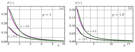
Figure 4: (Color online) Distribution function, $F(\tau)$, of the waiting times in the multiple-trapping model is shown with purple lines for the densities of tail states of the form $g(\varepsilon)\propto\exp\left[-\left(|\varepsilon|/{\cal T}_{0}\right)^{p}\right]$ with $p=1$ (a) and $p=1.8$ (b). Green lines are the interpolations of $F(\tau)$ with the form Eq. (8) of the main text.

VI Acknowledgements

We gratefully acknowledge numerous discussions with V. V. Dobrovitski. The work at the University of Utah was supported by NSF MRSEC program under Grant No. DMR 1121252. The work at Ames Laboratory was supported by the Department of Energy Basic EnergySciences under Contract No. DE-AC02-07CH11358.

Appendix A Applicability of the waiting times distribution Eq. (8) to the multiple trapping model

In the multiple trapping modelDT1 ; DT2 ; DT3 ; DT4 ; Harmon1 ; Harmon2 ; Baranovskii , the waiting time is determined by activation of electron from a localized state in the tail to the conduction band. If the energy position of the localized state is $-\varepsilon$, then the activation rate is equal to $\Gamma(\varepsilon)=\Gamma_{0}\exp[\varepsilon/{\cal T}]$, where ${\cal T}$ is the temperature. Actual waiting times, $t_{i}$, are random. While the average waiting time is $\Gamma^{-1}$, the distribution of the waiting times for a given $\varepsilon$ is given by the Poisson distribution

$$f_{\varepsilon}(\tau)=\Gamma(\varepsilon)\exp\left[-\Gamma(\varepsilon)\tau\right].$$ (51)

The remaining task is to average $f_{\varepsilon}(\tau)$ over $\varepsilon$ with the weight determined by the density of the tail states, $g(\varepsilon)$. In the multiple trapping model the form of $g(\varepsilon)$ is a simple exponent $g(\varepsilon)\propto\exp\left[\varepsilon/{\cal T}_{0}\right]$. The final expression for the waiting times distribution reads

$$F(\tau)\propto\int\limits_{-\infty}^{0}d\varepsilon g(\varepsilon)f_{\varepsilon}(\tau)\propto\frac{\alpha}{\tau^{\alpha+1}}\int\limits_{0}^{\Gamma_{0}\tau}dx~{}x^{\alpha}e^{-x},$$ (52)

where $\alpha={\cal T}/{\cal T}_{0}$. For large waiting times $\tau\gg\Gamma_{0}^{-1}$, we have $F(\tau)\propto\tau^{-(\alpha+1)}$. At $\tau\rightarrow 0$ the power-law divergence is cut off. The character of cutoff is not precisely the one given by Eq. (8), but they match very closely, as illustrated in the Figure 4. In organic semiconductors the density of the tail states is better approximated by a stretched-exponential form $g(\varepsilon)\propto\exp\left[-\left(|\varepsilon|/{\cal T}_{0}\right)^{p}\right]$, with $p$ close to $2$, see Refs. Baranovskii1, ; Baranovskii2, ; Robert, . Repeating the above steps for this $g(\varepsilon)$ we found that $F(\tau)$ can still be closely approximated with Eq. (8), see Figure 4.

References

(1)
P. W. Anderson and P. R. Weiss,
Rev. Mod. Phys. 25, 269 (1953).
(2) M. I. Dyakonov and V. I. Perel, Sov. Phys. Solid State 13,
3023 (1971).
(3)
H. Scher and E. W. Montroll, Phys. Rev. B 12, 2455 (1975).
(4) J. Noolandi,
Phys. Rev. B 16, 4466 (1977).
(5) T. Tiedje, J. M. Cebulka, D. L. Morel, and B. Abeles,
Phys. Rev. Lett. 46, 1425 (1981).
(6) B. Hartenstein, H. Bässler, A. Jakobs, and K. W. Kehr,
Phys. Rev. B 54, 8574 (1996).
(7) N. J. Harmon and M. E. Flatte, Phys. Rev. Lett. 110, 176602 (2013).
(8) N. J. Harmon and M. E. Flatte, Phys. Rev. B 90, 115203 (2014).
(9)
S. D. Baranovskii, Phys. Stat. Sol. (b) 251, 487 (2014).
(10)J. R. Klauder and P. W. Anderson,
Phys. Rev. 125, 912 (1962).
(11)
P. A. Bobbert, W. Wagemans, F.W. A. van Oost, B.
Koopmans, and M. Wohlgenannt, Phys. Rev. Lett. 102,
156604 (2009). T. D. Nguyen, G. Hukic-Markosian, F. Wang, L. Wojcik,
X.-G. Li, E. Ehrenfreund, and Z. V. Vardeny, Nat. Mater. 9,
345 (2010).
(12) R. Czech and K. W. Kehr, Phys. Rev. Lett. 53, 1783
(1984); Phys. Rev. B 34, 261 (1986).
(13)
R. C. Roundy and M. E. Raikh,
Phys. Rev. B 90, 201203(R) (2014).
(14)
V. V. Mkhitaryan and V. V. Dobrovitski,
Phys. Rev. B 92 054204 (2015).
(15) K. W. Kehr, G. Honig, and D. Richter,
Z. Phys. B 32, 49 (1978).
(16)
S. D. Baranovskii, H. Cordes, F. Hensel, and G. Leising, Phys. Rev. 62, 7934 (2000).
(17)
J. O. Oelerich, D. Huemmer, and S. D. Baranovskii, Phys. Rev. Lett. 108, 226403 (2012).
(18)R. C. Roundy and M. E. Raikh
Phys. Rev. B 90, 241202(R) (2014).