Network Clustering via Maximizing Modularity:
Approximation Algorithms and Theoretical Limits

Abstract

Many social networks and complex systems are found to be naturally divided into clusters of densely connected nodes, known as community structure (CS). Finding CS is one of fundamental yet challenging topics in network science. One of the most popular classes of methods for this problem is to maximize Newman’s modularity. However, there is a little understood on how well we can approximate the maximum modularity as well as the implications of finding community structure with provable guarantees. In this paper, we settle definitely the approximability of modularity clustering, proving that approximating the problem within any (multiplicative) positive factor is intractable, unless P = NP. Yet we propose the first additive approximation algorithm for modularity clustering with a constant factor. Moreover, we provide a rigorous proof that a CS with modularity arbitrary close to maximum modularity $Q_{OPT}$ might bear no similarity to the optimal CS of maximum modularity. Thus even when CS with near-optimal modularity are found, other verification methods are needed to confirm the significance of the structure.

I Introduction

Many complex systems of interest such as the Internet, social, and biological relations, can be represented as networks consisting a set of nodes which are connected by edges between them. Research in a number of academic fields has uncovered unexpected structural properties of complex networks including small-world phenomenon [1], power-law degree distribution, and the existence of community structure (CS) [2] where nodes are naturally clustered into tightly connected modules, also known as communities, with only sparser connections between them. Finding this community structure is a fundamental but challenging problem in the study of network systems and has not been yet satisfactorily solved, despite the huge effort of a large interdisciplinary community of scientists working on it over the past years [3].

Newman-Girvan’s modularity that measures the “strength” of partition of a network into modules (also called communities or clusters) [2] has rapidly become an essential element of many community detection methods. Despite of the known drawbacks [4, 5], modularity is by far the most used and best known quality function, particularly because of its successes in many social and biological networks [2] and the ability to auto-detect the optimal number of clusters [6, 7]. One can search for community structure by looking for the divisions of a network that have positive, and preferably large, values of the modularity. This is the underlying “assumption” for numerous optimization methods that find communities in the network via maximizing modularity (aka modularity clustering) as surveyed in [3]. However, there is a little understood on the complexity and approximability of modularity clustering besides its NP-completeness [8, 9] and APX-hardness [10]. The approximability of modularity clustering in general graphs remains an open question.

This paper focuses on understanding theoretical aspects of CSs with near-optimal modularity. Let $\mathcal{C}^{*}$ be a CS with maximum modularity value and let $Q_{OPT}$ be the modularity value of $\mathcal{C}^{*}$. Given $0<\rho<1$, polynomial-time algorithms that can find CSs with modularity at least $\rho Q_{OPT}$ are called (multiplicative) approximation algorithms; and $\rho$ is called (multiplicative) approximation factor. Given the NP-completeness of modularity clustering, we are left with two choices: designing heuristics which provides no performance guarantee (like the vast major modularity clustering works) or designing approximation algorithms which can guarantee near-optimal modularity.

We seek the answers to the following questions: how well we can approximate the maximum modularity, i.e., for what values of $\rho$ there exist $\rho$-approximation algorithms for modularity clustering? Moreover, do CSs with near-optimal modularity bear similarity to $\mathcal{C}^{*}$, the ultimate target of all modularity clustering algorithms? Our contributions (answers to the above questions) are as follows.

• We prove that there is no approximation algorithm with any factor $\rho>0$ for modularity clustering, unless P = NP, therefore definitively settling the approximation complexity of the problem. We prove this intractability results for both weighted networks and unweighted networks (with the allowance of multiple edges.)

• On the bright side, we propose the first additive approximation algorithm that find a community structure with modularity at least $Q_{OPT}-2(1-\kappa)$ for $\kappa=0.766$. The proposed algorithm also provides better quality solutions comparing to the-state-of-the-art modularity clustering methods.

• We provide rigorous proof that CSs with near-optimal modularity might be completely different from $\mathcal{C}^{*}$, the CS with maximum modularity $Q_{OPT}$. This holds no matter how close the modularity value to $Q_{OPT}$ is. Thus adopters of modularity clustering should carefully employ other verification methods even when they found CSs with modularity values that are extremely close to the optimal ones.

Related work. A vast amount of methods to find community structure is surveyed in [3]. Brandes et al. proves the NP-completeness for modularity clustering, the first hardness result for this problem. The problem stands NP-hard even for trees [9]. DasGupta et al. show that modularity clustering is APX-hard, i.e., there exists a constant $c>1$ so that there is no (multiplicative) $c$-approximation for modularity clustering unless P=NP [10]. In this paper, we show a much stronger result that the inapproximability holds for all $c>1$.

Modularity has several known drawbacks. Fortunato and Barthelemy [4] has shown the resolution limit, i.e., modularity clustering methods fail to detect communities smaller than a scale, the resolution limit only appears when the network is substantially large [11]. Another drawback is modularity’s highly degenerate energy landscape [5], which may lead to very different partitions with equally high modularity. However, for small and medium networks of several thousand nodes, the Louvain method [12] to optimize modularity is among the best algorithms according to the LFR benchmark [11]. The method is also adopted in products such as LinkedIn InMap or Gephi.

While approximation algorithms for modularity clustering in special classes of graphs are proposed for scale-free networks[13, 14] and $d$-regular graphs [10], no such algorithms for general graphs are known.

Organization. We present terminologies in Section II. The inapproximability of modularity clustering in weighted and unweighted networks is presented in Section III. We present the first additive approximation algorithm for modularity clustering in Section IV. Section V illustrates that the optimality of modularity does not correlate to the similarity between the detected CS and the maximum modularity CS. Section VI presents computational results and we conclude in Section VII.

II Preliminaries

We consider a network represented as an undirected graph $G=(V,E)$ consisting of $n=|V|$ vertices and $m=|E|$ edges. The adjacency matrix of $G$ is denoted by $\bm{A}=\left(A_{ij}\right)$, where $A_{ij}$ is the weight of edge $(i,j)$ and $A_{ij}=0$ if $(i,j)\notin E$. We also denote the (weighted) degree of vertex $i$, the total weights of edges incident at $i$, by $\textsf{deg}(i)$ or, in short, $d_{i}$.

Community structure (CS) is a division of the vertices in $V$ into a collection of disjoint subsets of vertices $\mathcal{C}=\left\{C_{1},C_{2},\ldots,C_{l}\right\}$ that the union gives back $V$. Especially, the number of communities $l$ is not known as a prior. Each subset $C_{i}\subseteq V$ is called a community (or module) and we wish to have more edges connecting vertices in the same communities than edges that connect vertices in different communities. In this paper, we shall use the terms community structure and clustering interchangeably.

The modularity [15] of $\mathcal{C}$ is defined as

$$Q(\mathcal{C})=\frac{1}{2M}\displaystyle\sum_{i,j\in V}\left(A_{ij}-\frac{d_{i}d_{j}}{2M}\right)\delta_{ij}$$ (1)

where $d_{i}$ and $d_{j}$ are degree of nodes $i$ and $j$, respectively; $M$ is the total edge weights; and the element $\delta_{ij}$ of the membership matrix $\bm{\delta}$ is defined as

$$\delta_{ij}=\begin{cases}1,&\mbox{if }i\mbox{ and }j\mbox{ are in the same community}\\ 0,&\mbox{otherwise}.\end{cases}.$$

The modularity values can be either positive or negative and it is believed that the higher (positive) modularity values indicate stronger community structure. The modularity clustering problem asks to find a division which maximizes the modularity value.

Let $\bm{B}$ be the modularity matrix [15] with entries

$$B_{ij}=A_{ij}-\frac{d_{i}d_{j}}{2M}.\text{ We have }Q(\mathcal{C})=\frac{1}{2M}\sum_{i,j}B_{ij}\delta_{ij}.$$

Alternatively the modularity can also be defined as

$$Q(\mathcal{C})=\displaystyle\sum_{t=1}^{l}\left(\frac{E(C_{t})}{M}-\frac{vol(C_{t})^{2}}{4M^{2}}\right),$$ (2)

where $E(C_{t})$ is the total weight of the edges inside $C_{t}$ and $vol(C_{t})=\sum_{v\in C_{t}}d_{v}$ is the volume of $C_{t}$.

III Multiplicative Approx. Algorithm

A major thrust in optimization is to develop approximation algorithms of which one can theoretically prove the performance bound. Designing approximation algorithms is, however, very challenging. Thus, it is desirable to know for what values of $\rho$, there exist $\rho$-approximation algorithms. This section gives a negative answer to the existence of approximation algorithms for modularity clustering with any (multiplicative) factor $\rho>0$, unless P $=$ NP.

We show the inapproximability result for weighted networks via a gap-producing redution from the PARTITION problem in subsection III-A. Ignoring the weights doesn’t make the problem any easier to approximate, as we shall show in subsection III-B that the same inapproximability hold for unweighted networks.

Our proofs for both cases use the fact that we can approximate modularity clustering if and only if we can approximate the problem of partitioning the network into two communities to maximize modularity. Then we show that the later problem cannot be approximated within any finite factor.

III-A  Inapproximability in Weighted Graphs

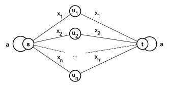
Figure 1: Gap-producing reduction from PARTITION to modularity clustering. There exists a community structure of positive modularity if and only if we can divide the integers $x_{1},\ldots,x_{n}$ into two halves with equal sum.

Theorem 1

For any $\rho>0$, there is no polynomial-time algorithm to find a community structure with a modularity value at least $\rho Q_{OPT}$, unless P$=$NP. Here $Q_{OPT}$ denotes the maximum modularity value among all possible divisions of the network into communities.

Proof:

We present a gap-producing reduction [16] that maps an instance $\Phi$ of the following problem

PARTITION: Given integers $x_{1},x_{2},\ldots,x_{n}$, can we divide the integers into two halves with equal sum?

to a graph $\tilde{G}=(\tilde{V},\tilde{E})$ such that

• If $\Phi$ is an YES instance, i.e., we can divide $x_{i}$ into two halves with equal sum, then $Q_{OPT}(\tilde{G})>0$.

• If $\Phi$ is a NO instance, then $Q_{OPT}(\tilde{G})=0$.

Reduction: The graph $\tilde{G}$ is shown in Fig. 1. $\tilde{G}$ consists of two special nodes $s$ and $t$ and $n$ middle nodes $u_{1},u_{2},\ldots,u_{n}$. Each $u_{i}$ is connected to both $s$ and $t$ with edges of weights $x_{i}$. Let $K=\frac{1}{2}\sum_{t=1}^{n}x_{t}$. Both $s$ and $t$ have self-loops of weights $a=\frac{1}{8K+2}$. The total weights of edges in $\tilde{G}$ is

$$\tilde{M}=2\sum_{t=1}^{n}x_{t}+2a=4K+2a.$$

This reduction establishes the NP-hardness of distinguish graphs having a community structure of positive modularity from those having none. An approximation algorithm with a guarantee $\rho>0$ or better, will find a community structure of modularity at least $\rho Q_{OPT}(\tilde{G})>0$, when given a graph from the first class. Thus, it can distinguish the two classes of graphs, leading to a contradiction to the NP-hardness of PARTITION [17].

($\bm{\rightarrow}$) If $\Phi$ is an YES instance, there exists a partition of $\{1,2,\ldots,n\}$ into disjoint subsets $S_{1}$ and $S_{2}$ such that

$$\sum_{i\in S_{1}}x_{i}=\sum_{j\in S_{2}}x_{j}=\frac{1}{2}\sum_{t=1}^{n}x_{t}=K,$$

Consider a CS $\tilde{\mathcal{C}}$ in $\tilde{G}$ that consists of two communities $C_{1}=\{s\}\cup\{u_{i}|i\in S_{1}\}$ and $C_{2}=\{t\}\cup\{u_{j}|j\in S_{2}\}$. We have $vol(C_{1})=vol(C_{2})=\tilde{M}$. From (2), the modularity value of $\tilde{C}$ is

$$Q(\tilde{\mathcal{C}})=\frac{2K+2a}{\tilde{M}}-\frac{2\tilde{M}^{2}}{4\tilde{M}^{2}}=\frac{a}{\tilde{M}}>0$$

Thus $Q_{OPT}\geq Q_{\tilde{\mathcal{C}}}>0$.

($\bm{\leftarrow}$) If $\Phi$ is a NO instance, we prove by contradiction that $Q_{OPT}=0$. Assume otherwise $Q_{OPT}>0$. Let $Q_{2}$ denote the maximum modularity value among all partitions of $\tilde{G}$ into (at most) two communities. It is known from [13] that

$$Q_{2}\geq\frac{1}{2}Q_{OPT}.$$

Thus there exists a community $\hat{\mathcal{C}}$ of modularity value $Q_{2}\geq\frac{1}{2}Q_{OPT}>0$ such that $\hat{\mathcal{C}}$ has exactly two communities, say $\hat{C}_{1}$ and $\hat{C}_{2}$. Let $\delta(\hat{C}_{1})$ be the total weights of edges crossing between $\hat{C}_{1}$ and $\hat{C}_{2}$. We have

$$Q_{2}=\frac{\tilde{M}-\delta(\hat{C}_{1})}{\tilde{M}}-\frac{vol(\hat{C}_{1})^{2}+vol(\hat{C}_{2})^{2}}{4\tilde{M}^{2}}.$$

Substitute $2\tilde{M}=vol(\hat{C}_{1})+vol(\hat{C}_{2})$ and simplify

$$Q_{2} =\frac{1}{4\tilde{M}^{2}}\left(2vol(\hat{C}_{1})vol(\hat{C}_{2})-4\tilde{M}\delta(\hat{C}_{1})\right)$$ (3)

$$=\frac{vol(\hat{C}_{1})vol(\hat{C}_{2})}{2\tilde{M}^{2}}\Big{(}1-\Big{[}\frac{\delta(\hat{C}_{1})}{vol(\hat{C}_{1})}+\frac{\delta(\hat{C}_{1})}{vol(\hat{C}_{2})}\Big{]}\Big{)}$$

Since $Q_{2}>0$, we have

$$\frac{\delta(\hat{C}_{1})}{vol(\hat{C}_{1})}+\frac{\delta(\hat{C}_{1})}{vol(\hat{C}_{2})}<1.$$ (4)

We show that $s$ and $t$ cannot be in the same community. Otherwise, assume $s$ and $t$ belong to $\hat{C}_{1}$, then $\hat{C}_{2}$ contains only nodes from $\{u_{1},u_{2},\ldots,u_{n}\}$. Thus

$$vol(\hat{C}_{2})=\delta(\hat{C}_{1})=2\sum_{u_{j}\in\hat{C}_{2}}x_{j}.$$

It follows that $\frac{\delta(\hat{C}_{1})}{vol(\hat{C}_{2})}=1$, which contradicts (4).

Since $s$ and $t$ are in different communities, whether we assign $u_{i}$ into $\hat{C}_{1}$ or $\hat{C}_{2}$, it always contributes to $\delta(\hat{C}_{1})$ an amount $x_{i}$. Therefore

$$\delta(\hat{C}_{1})=\sum_{t=1}^{n}x_{t}=2K=\frac{1}{2}\tilde{M}-a.$$

Since $\Phi$ is a NO instance, the integrality of $x_{i}$ leads to

$$vol(\hat{C}_{1})-vol(\hat{C}_{2})=2\left(\sum_{u_{i}\in C_{1}}x_{i}-\sum_{u_{j}\in C_{2}}x_{j}\right)\geq 2.$$

Moreover, $a=\frac{1}{8K+2}<\frac{1}{2\hat{M}}$. Thus we have

$$\frac{\delta(\hat{C}_{1})}{vol(\hat{C}_{1})}+\frac{\delta(\hat{C}_{1})}{vol(\hat{C}_{2})}\geq\delta(\hat{C}_{1})\left(\frac{1}{\tilde{M}-1}+\frac{1}{\tilde{M}+1}\right)$$

$$= \frac{(\frac{1}{2}\tilde{M}-a)2\tilde{M}}{\tilde{M}^{2}-1}>\frac{\tilde{M}^{2}-2\frac{1}{2\tilde{M}}\tilde{M}}{\tilde{M}^{2}-1}=1,$$

which contradicts (4).

Hence if $\Phi$ is a NO instance, then $Q_{OPT}=0$.∎

III-B  Inapproximability in Unweighted Graphs

This section shows that it is NP-hard to decide whether one can divide an unweighted graph into communities with (strictly) positive modularity score. Thus approximating modularity clustering is NP-hard for any positive approximation factor. Our proof reduces from the unweighted Max-Cut problem, which is NP-hard even for 3-regular graphs [18]. Our reduction is explicit and can be used to generate hard instances for modularity clustering problem, as shown in Section VI.

Remark that one can replace weighted edges with multiple parallel edges in the reduction in Theorem 1 to get a reduction for unweighted graphs. However, such an approach does not yield a polynomial-time reduction, since instances of PARTITION can have items with exponentially large weights.

Theorem 2

Approximating modularity clustering within any positive factor in unweighted graphs (with the allowance of multiple edges) is NP-hard.

Proof:

We reduce from an instance $\Psi$ of the Max-Cut problem “whether an undirected unweighted graph $G=(V,E)$ has a subset $S\subseteq V$ of the vertices such that the size of the cut $\delta(S)=\{(u,v)\in E\ |\ u\in S,v\notin S\}$ is at least $k$?” to a graph $G^{\prime}=(V^{\prime},E^{\prime})$ such that

• If the answer to $\Psi$ is YES, i.e., there exists a cut $S$ with $\delta(S)\geq k$, then $Q_{OPT}(G^{\prime})>0$.

• If the answer to $\Psi$ is NO, $Q_{OPT}(G^{\prime})=0$.

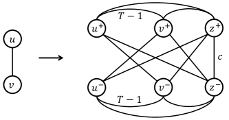
Figure 2: Reduction for a sample network with an edge connecting two nodes. The multiplicity of edges in the right network is $T=n^{4}$ unless otherwise noted.

Using the same arguments in the proof of Theorem 1, the above reduction leads to the NP-hardness of approximating modularity clustering within any positive finite factor in unweighted graphs.

Our reduction is similar to the reduction from Max-Cut in [18]. An example is given in Fig. 2. For each vertex $v\in V$, we add two vertices $v^{+}$ and $v^{-}$ into $V^{\prime}$. Also we add two special vertices $z^{+}$ and $z^{-}$ into $V^{\prime}$. Thus $V^{\prime}=\{v^{+},v^{-}\ |\ v\in V\}\cup\{z^{+},z^{-}\}$. Next choose a large integer constant $T=n^{4}$, where $n=|V|$. We connect vertices in $G^{\prime}$ in the following orders:

• For each edge $(u,v)\in E$, connect $u^{+}$ to $v^{+}$ and $u^{-}$ to $v^{-}$, each using $T-1$ parallel edges.

• There are no edges between $u^{+}$ and $u^{-}$ for all $u\in V$. Connect $z^{+}$ to $z^{-}$ using $c$ parallel edges, where $c=4k-2m-1$ (and $m=|E|$).

• Connect the remaining pairs of vertices, each using $T$ parallel edges.

Feasibility of Reduction. Obviously, the reduction has a polynomial size. Denote by $n^{\prime}$ and $m^{\prime}$ the number of vertices and edges in $G^{\prime}$, respectively. We have

$$n^{\prime}=2n+2\text{ and }m^{\prime}=2n(n+1)T-2m+c.$$

We also need to verify that $c\geq 0$. By [19], we can always find in $G$ a cut of size at least $\frac{m}{2}+2$, thus we can distinguish trivial instances of Max-Cut with $k\leq\frac{m}{2}+2$ from the rest in a polynomial time. For non-trivial instances of Max-Cut, i.e., $k>\frac{m}{2}+2$ we have $4k-2m-1>4(\frac{m}{2}+2)-2m-1>0$.

($\bm{\rightarrow}$) If $\Psi$ is an YES instance, there exists a cut $(S\subseteq V,\bar{S}=V\setminus S)$ satisfying $\delta_{G}(S)\geq k$. Let $S^{+}=\{v^{+}|\ v\in S\},\bar{S}^{+}=\{v^{+}|\ v\notin S\},S^{-}=\{v^{-}|\ v\in S\},$ and $\bar{S}^{-}=\{v^{-}|\ v\notin S\}$. Construct a CS $\mathcal{C}=\{C_{1},C_{2}\}$ of $G^{\prime}$ in which

$$C_{1}=S^{+}\cup\bar{S}^{-}\cup\{z^{+}\},C_{2}=S^{-}\cup\bar{S}^{+}\cup\{z^{-}\}.$$

We will prove that $Q(\mathcal{C})>0$. By Eq. (3),

$$Q(\mathcal{C})=\frac{1}{4m^{\prime 2}}\left(2vol(C_{1})vol(C_{2})-4m^{\prime}\delta_{G^{\prime}}(C_{1})\right)$$ (5)

Observe that $d_{v^{+}}=d_{v^{-}}=2nT-d_{v},\forall v\in V$ and both communities $C_{1}$ and $C_{2}$ either contains $v^{+}$ or $v^{-}$ but not both. The same observation holds for the vertices $z^{+}$ and $z^{-}$ that have degrees $2nT+c$. Thus

$$vol(C_{1})=vol(C_{2})=m^{\prime}.$$ (6)

To compute $\delta_{G^{\prime}}(C_{1})$, we recall that the nodes in $C_{1}$ connect to those in $C_{2}$, each with $T$ parallel edges with the exceptions of the following pairs:

• $2\delta_{G}(S)$ pairs of nodes between $(S^{+},\bar{S}^{+})$ and $(S^{-},\bar{S}^{-})$, each connected with $T-1$ parallel edges

• $z^{+}$ connects to $z^{-}$ with only $c$ parallel edges.

Hence, we have

$$\delta_{G^{\prime}}(C_{1}) =n(n+1)T-2\delta_{G}(S)+c$$

$$\leq n(n+1)T-2k+c.$$ (7)

Substitute Eqs. (6) and (7) into (5), we have

$$Q(\mathcal{C})=\frac{1}{4m^{\prime 2}}(2m^{\prime 2}-4m^{\prime}\delta_{G^{\prime}}(C_{1}))=\frac{m^{\prime}-2\delta_{G^{\prime}}(C_{1})}{2m^{\prime}}$$

$$\geq\frac{1}{2m^{\prime}}\Big{(}2n(n+1)T-2m+c$$

$$\quad\quad-2n(n+1)T+4k-2c\Big{)}=\frac{1}{2m^{\prime}}>0.$$

Thus $Q_{OPT}\geq Q_{\mathcal{C}}>0$.

($\bm{\leftarrow}$) If $\Psi$ is a NO instance, we prove by contradiction that $Q_{OPT}=0$. Assume otherwise $Q_{OPT}>0$. Let $Q_{2}$ denote the maximum modularity value among all partitions of $G^{\prime}$ into (at most) two communities and $\mathcal{C}=\{C_{1},C_{2}\}$ be a community structure of $G^{\prime}$ with the modularity value $Q_{2}\geq\frac{1}{2}Q_{OPT}>0$ [13]. We will show that $Q_{2}\leq 0$, hence, a contradiction. Assume that $y=|C_{1}|\leq|C_{2}|$, consider the following two cases:

Case $y<n+1$: Since $d_{v^{+}}=d_{v^{-}}=2nT-d_{v},\forall v\in V$ and $d_{z^{+}}=d_{z^{-}}=2nT+c$, we have

$$vol(C_{1})\leq 2nTy+2c$$

Since $vol(C_{1})+vol(C_{2})=2m^{\prime}$, it follows that

$$vol(C_{1})vol(C_{2})\leq(2nTy+2c)(2m^{\prime}-(2nTy+2c)).$$

Moreover, using the same arguments that leads to Eq. 7, we have

$$\delta_{G^{\prime}}(C_{1})\geq y(2n+2-y)T-yT=yT(2n+1-y).$$

Here the factor $yT$ arises from the fact that there are at most $y$ pairs of $(v^{+},v^{-})$ that across $C_{1}$ and $C_{2}$.

Thus we obtain from (5) the following inequality

$$Q(\mathcal{C})=\frac{1}{4m^{\prime 2}}\left(2vol(C_{1})vol(C_{2})-4m^{\prime}\delta_{G^{\prime}}(C_{1})\right)$$

$$\leq\frac{1}{2m^{\prime 2}}\Big{(}(2nTy+2c)(2m^{\prime}-(2nTy+2c))$$

$$\quad\quad\quad\quad-2m^{\prime}yT(2n+1-y)\Big{)}.$$

After some algebra and applying the inequalities $y~{}\leq~{}n$ and $c\leq 2n^{2}$, we obtain

$$Q(\mathcal{C})\leq\frac{2T^{2}ny}{m^{\prime 2}}\left(-(n+1-y)+\frac{O(n^{3})}{T}\right)<0.$$

Case $y=|C_{1}|=|C_{2}|=n+1$: We bound $\delta_{G^{\prime}}(C_{1})$ by considering two sub-cases:

• If there is some $v\in V$ such that $v^{+},v^{-}\in C_{1}$ or $z^{+},z^{-}\in C_{1}$, then $\delta_{G^{\prime}}(C_{1})\geq(n+1)(n+1)T-nT-(n+1)(n+1)$

• Otherwise, all pairs $v^{+}$ and $v^{-}$ (as well as $z^{+}$ and $z^{-}$) are in different sides of the cut $C_{1}$. Thus $C_{1}$ induces in $G$ a cut $S\subseteq V$. Then $\delta_{G^{\prime}}(C_{1})\geq n(n+1)T-2\delta_{G^{\prime}}(S)+c\geq n(n+1)T-2(k-1)+c$, as $\delta(S)<k$.

As $n(n+1)T+T-(n+1)^{2}\geq n(n+1)T-2(k-1)+c$, it holds for the both cases that

$$\delta_{G^{\prime}}(C_{1})\geq n(n+1)T-2(k-1)+c.$$

Since

$$vol(C_{1})vol(C_{2})\leq m^{\prime 2},$$

using Eq. (5), we obtain

$$Q(\mathcal{C})\leq\frac{1}{4m^{\prime 2}}\left(2m^{\prime 2}-4m^{\prime}\left(n(n+1)T-2(k-1)+c\right)\right)$$

$$\leq\frac{1}{2m^{\prime}}\Big{(}2n(n+1)T-2m+c$$

$$\quad\quad-2n(n+1)T+4k-4-2c\Big{)}=\frac{-3}{2m^{\prime}}<0.$$

Thus if $\Psi$ is a NO instance, then $Q_{OPT}=0$. ∎

IV Additive Approx. Algorithm

We propose the first additive approximation algorithm that find a community structure $\mathcal{C}$ satisfying the following performance guarantee

$$Q(\mathcal{C})\geq Q_{OPT}-2(1-\kappa),$$ (8)

where $\kappa=0.766$. The algorithm is based on rounding a semidefinite programm, similar to that in [20] for the Max-Agree problem.

First, we formulate modularity clustering as a vector programming. Let $e_{j}\in\mathbb{R}^{n}$ be the unit vector with $1$ in the $i^{\text{th}}$ coordinate and $0$s everywhere else. Let $x_{i}\in\{e_{1},e_{2},\ldots,e_{n}\}$ be the variable that indicates the community of vertex $i$, i.e., if $x_{i}=e_{j}$ then vertex $i$ belongs to community $j$. The vector programming is as follows.

$$\max\quad \frac{1}{2M}\sum_{i,j}B_{ij}\quad x_{i}\cdot x_{j}$$ (9)

$$x_{i}\in\{e_{1},e_{2},\ldots,e_{n}\}\quad\forall i,$$ (10)

where $(\cdot)$ denotes the inner product (or dot product).

We relax the constraint $x_{i}\in\{e_{1},e_{2},\ldots,e_{n}\}$ to get a semidefinite program (SDP) with new constraints

$$x_{i}\cdot x_{i}=1\quad\forall i$$ (11)

$$x_{i}\cdot x_{j}\geq 0\quad\forall i\neq j$$ (12)

$$x_{i}\in\mathbb{R}^{n}\quad\forall i.$$ (13)

One of the reason that modularity clustering resists approximation approaches such as semidefinite rounding is that the matrix $\bm{B}$ contains both negative and nonnegative entries. Indeed, all entries in $\bm{B}$ sum up to zero [15]. To overcome this, we add a fixed amount $\frac{W}{2M}$ to the objective of SDP, where

$$W=\sum_{(i,j)\in\bm{B}^{+}}B_{ij}=|\sum_{(i,j)\in\bm{B}^{-}}B_{ij}|\text{ with }$$

$$\bm{B}^{+}=\{(i,j)\ |\ B_{ij}\geq 0\}\text{ and }\bm{B}^{-}=\{(i,j)\ |\ B_{ij}<0\}.$$

The new objective is then

$$\frac{1}{2M}\Big{(}\sum_{i,j}B_{ij}x_{i}\cdot x_{j}-\sum_{(i,j)\in\bm{B}^{-}}B_{ij}\Big{)}$$

$$= \frac{1}{2M}\Big{(}\sum_{(i,j)\in\bm{B}^{+}}B_{ij}x_{i}\cdot x_{j}+\sum_{(i,j)\in\bm{B}^{-}}B_{ij}(x_{i}\cdot x_{j}-1)\Big{)}$$

$$= \frac{1}{2M}\big{(}\sum_{(i,j)\in\bm{B}^{+}}B_{ij}x_{i}\cdot x_{j}+\sum_{(i,j)\in\bm{B}^{-}}-B_{ij}(1-x_{i}\cdot x_{j})\big{)}.$$

Note that all of coefficients in the new objective are nonnegative. Thus we transform the modularity clustering problem to an SDP of the Max-Agree problem [20] which can be solved using the rounding procedure in [20]. Our additive approximation algorithm can be summarized as follows.

Algorithm 1 SDP to Maximize Modularity (SDPM)

1:Solve the SDP relaxation in (9) and (11)-(13)

2:Choose $k$ random hyperplanes, and use projection to divide the set of vertices into $2^{k}$ clusters.

3:Return the better clustering $\mathcal{C}$ of $k=2$ and $k=3$.

Since all coefficients in the new objective are positive and the fixed factor $\frac{W}{2M}$ does not affect the solution of SDP. We can apply Theorem 3 in [20] to obtain

$$Q_{G}(\mathcal{C})+\frac{W}{2M}\geq\kappa\Big{(}Q_{OPT}+\frac{W}{2M}\Big{)},$$ (14)

where $\kappa=0.766$ is the approximation factor for the generalized Max-Agree problem [20].

Since $\frac{W}{2M}<1$ and $Q_{OPT}<1$, we can simplify (14) to yield the following theorem.

Theorem 3

Given graph $G$, there is a polynomial-time algorithm that finds a community structure $\mathcal{C}$ of $G$ satisfying

$$Q_{G}(\mathcal{C})>\kappa Q_{OPT}-(1-\kappa),$$

and

$$Q_{G}(\mathcal{C})>Q_{OPT}-2(1-\kappa).$$

where $\kappa=0.766$.

Apparently, the higher $\kappa$ the better the performance guarantee. Any improvement on the approximation factor for the generalized Max-Agree problem will immediately lead to the improvement in the approximation factor for modularity clustering.

V Do Small Gaps Guarantee Similarity?

Given $0<a<b<1$ and an arbitrary graph $G$, we show how to construct a “structurally equivalent” graph $G^{\prime}$ of $G$ in which community structures have modularity values between $a$ and $b$. Multiple implications of this finding include:

• There are graphs of any size that have clustering with extremely small modularity (e.g. by choosing $a$ and $b$ close to zero.) This gives additional light into why it is hard to distinguish between graphs having no community structure with positive modularity and the others (Section III-A.)

• There are graphs of any size that all “reasonable” clustering of the network yields modularity values in range $(a(1-\epsilon),a)$ for arbitrary small $\epsilon>0$ and any $0<a<1-\epsilon$. Thus even we find a CS with modularity at least $(1-\epsilon)Q_{OPT}$ or $Q_{OPT}-\epsilon$, the obtained CS can be completely different from $\mathcal{C}^{*}$, the maximum modularity CS.

Therefore, the presence of high modularity clusters neither indicates the presence of community structure nor how easy it is to detect such a structure if it exists.

We present our construction which consists of two transformations, namely $\alpha$-transformation and $(\tau,k)$-transformation.

$\alpha$-transformation: An $\alpha$-transformation with $0<\alpha\leq 1$ maps each graph $G=(V,E)$ with an “equivalent” graph $G^{\prime}=T_{\alpha}(G)$ and maps (one-to-one correspondence) each CS $\mathcal{C}$ of $G$ to a CS $\mathcal{C}^{\prime}$ of $G^{\prime}$ that satisfies

$$Q_{G^{\prime}}(\mathcal{C}^{\prime})=\alpha Q_{G}(\mathcal{C}),$$

where $Q_{G^{\prime}}(\mathcal{C}^{\prime})$ and $Q_{G}(\mathcal{C})$ denote the modularity of $\mathcal{C}^{\prime}$ in $G^{\prime}$ and $\mathcal{C}$ in $G$, respectively.

Construction: $G^{\prime}$ also has $V$ as the set of vertices. The weighted adjacency matrix $A^{\prime}$ of $G^{\prime}$ is defined as

$$A^{\prime}_{ij}=A_{ij}+\frac{1-\alpha}{\alpha}\frac{d_{i}d_{j}}{2M}.$$ (15)

We show in the following lemma that the same community induced by $\mathcal{C}$ in $G^{\prime}$ has modularity scaled down by a fraction $\alpha$.

Lemma 1

Given a community structure $\mathcal{C}$ of $G$, the CS $\mathcal{C}^{\prime}$ induced by $\mathcal{C}$ in $G^{\prime}=T_{\alpha}(G)$ satisfies

$$Q_{G^{\prime}}(\mathcal{C}^{\prime})=\alpha Q_{G}(\mathcal{C}).$$

Proof:

Let $\delta_{ij}=1$ if $i$ and $j$ are in the same community in $C$ and $\delta_{ij}=0$ otherwise. By definition

$$Q_{G^{\prime}}(\mathcal{C}^{\prime})=\frac{1}{2M^{\prime}}\sum_{i,j}\left(A_{ij}^{\prime}-\frac{d_{i}^{\prime}d_{j}^{\prime}}{2M^{\prime}}\right)\delta_{ij},$$

where $M^{\prime},d_{i}^{\prime}$, and $d_{j}^{\prime}$ are the total edge weights, weighted degree of $i$, and weighted degree of $j$ in $G^{\prime}$, respectively.

We have

$$d_{i}^{\prime} =\sum_{j\in V}A_{ij}^{\prime}=\sum_{j\in V}\left(A_{ij}+\frac{1-\alpha}{\alpha}\frac{d_{i}d_{j}}{2M}\right)$$

$$=\sum_{j\in V}A_{ij}+\frac{1-\alpha}{\alpha}d_{i}\sum_{j\in V}d_{j}/(2M)=\frac{1}{\alpha}d_{i}.$$ (16)

Moreover,

$$M^{\prime} =\frac{1}{2}\sum_{i\in V}d_{i}^{\prime}=\frac{1}{2\alpha}\sum_{i\in V}d_{i}=\frac{1}{\alpha}M.$$ (17)

From (15), (16), and (17), we have

$$Q_{G^{\prime}}(\mathcal{C}^{\prime}) =\frac{\alpha}{2M}\sum_{i,j}\left(A_{ij}+\frac{1-\alpha}{\alpha}\frac{d_{i}d_{j}}{2M}-\frac{d_{i}d_{j}}{2M\alpha}\right)\delta_{ij}$$

$$=\frac{\alpha}{2M}\sum_{i,j}\left(A_{ij}-\frac{d_{i}d_{j}}{2M}\right)\delta_{ij}=\alpha Q_{G}(\mathcal{C}).\$$

∎

$(\tau,k)$-transformation: A $(\tau,k)$-transformation with $0<\tau<1$ and $k\in\mathsf{Z}^{+}$ maps a graph $G=(V,E)$ with a graph $G^{\prime}=T_{\tau,k}(G)$ and maps each community structure $C$ in $G$ to a community structure $C^{\prime}$ in $G^{\prime}$ that satisfies

$$Q_{G^{\prime}}({\mathcal{C}^{\prime}})=\tau+(1-\tau-\epsilon)Q_{G}(\mathcal{C}),$$

where $\epsilon=\frac{(1-\sqrt{\tau})^{2}}{k}$.

Construction: The set of vertices $V^{\prime}$ is obtained by adding to $V$ $k$ isolated vertices $n+1,n+2,\ldots,n+k$. Let $\beta=\frac{1}{\sqrt{\tau}}-1$, i.e., $\tau=1/(1+\beta)^{2}$. We attach loops of weight $\frac{\beta}{2}d_{i}$ to vertices $1\leq i\leq n$ and loops of weight $\frac{\beta(\beta+1)}{k}M$ to $n+1,\ldots,n+k$. Thus the weighted adjacency matrix $A^{\prime}$ of $G^{\prime}$ is as follows.

$$A_{ij}^{\prime}=\begin{cases}A_{ij}&1\leq i\neq j\leq n\\ \frac{\beta}{2}d_{i}&1\leq i=j\leq n\\ \frac{1}{k}\beta(\beta+1)M&i=j>n\\ 0&\text{ otherwise }.\end{cases}$$ (18)

CS $\mathcal{C}^{\prime}$ of $G^{\prime}$ is obtained from $\mathcal{C}$ by adding $k$ singleton communities that contains only one node from $\{n+1,\ldots,n+k\}$.

Lemma 2

Given a community structure $\mathcal{C}$ of $G$, the community structure $\mathcal{C}^{\prime}$ induced by $\mathcal{C}$ in $G^{\prime}=T_{\tau,k}(G)$ satisfies

$$Q_{G^{\prime}}({\mathcal{C}^{\prime}})=\tau+(1-\tau-\epsilon)Q_{G}(\mathcal{C}),$$

where $\epsilon=\frac{(1-\sqrt{\tau})^{2}}{k}$.

Proof:

Since a loop contribute twice to the degree, we have

$$d_{i}^{\prime}=\sum_{j\neq i}A_{ij}+2\frac{\beta}{2}d_{i}=(1+\beta)d_{i},$$ (19)

and

$$d_{n+l}^{\prime}=\frac{2}{k}\beta(\beta+1)M,l=1..k.$$ (20)

Therefore

$$M^{\prime} =\frac{1}{2}\sum_{i\in V^{\prime}}d_{i}^{\prime}=\frac{1}{2}\left(\sum_{i\in V}d_{i}^{\prime}+k\frac{2}{k}\beta(\beta+1)M\right)$$

$$=(1+\beta)M+\beta(\beta+1)M=(\beta+1)^{2}M.$$ (21)

We have

$$Q_{G^{\prime}}(\mathcal{C}^{\prime})=\frac{1}{2M^{\prime}}\sum_{i,j\in V}\left(A_{ij}^{\prime}-\frac{d_{i}^{\prime}d_{j}^{\prime}}{2M^{\prime}}\right)\delta_{ij}$$

$$+\sum_{l=1}^{k}\left(\frac{\beta(\beta+1)M}{kM^{\prime}}-\frac{d_{n+l}^{\prime 2}}{4M^{\prime 2}}\right)\delta_{n+l,n+l}.$$

Substitute (19), (20), and (V) into the above equation

$$Q_{G^{\prime}}(\mathcal{C}^{\prime})=\frac{1}{2M(\beta+1)^{2}}\sum_{i,j\in V}\left(A_{ij}-\frac{d_{i}d_{j}}{2M}\right)\delta_{ij}$$

$$+\frac{\sum_{i\in V}\frac{\beta}{2}d_{i}}{M^{\prime}}+\left(\frac{\beta}{\beta+1}-\frac{\beta^{2}}{k(1+\beta)^{2}}\right)$$

$$=\frac{1}{(\beta+1)^{2}}Q_{G}(\mathcal{C})+1-\frac{1}{(\beta+1)^{2}}-\frac{\beta^{2}}{k(\beta+1)^{2}}$$

$$=\tau Q_{G}(\mathcal{C})+(1-\tau-\epsilon).$$

This yields the proof. ∎

Now we can combine the two transformations to “engineer” the modularity values into any desirable range $(a,b)$.

Theorem 4

Given a graph $G$, applying an $\alpha$-transformation on $G$, followed by a $(\tau,k)$-transformation yields a graph $\tilde{G}$ and a mapping from each community structure $C$ of $G$ to a community structure $\tilde{C}$ of $\tilde{G}$ that satisfies

$$Q_{\tilde{G}}(\tilde{\mathcal{C}})=\tau\alpha Q_{G}(\mathcal{C})+(1-\tau-\epsilon),$$

where $\epsilon=\frac{(1-\sqrt{\tau})^{2}}{k}$.

Since $-1/2<Q_{G}({\mathcal{C}})<1$ [13], setting $\tau=1-(\frac{2}{3}a+\frac{1}{3}b)$ and $\alpha=\frac{2}{3}(b-a)$ ensures that $a<Q_{\tilde{G}}(\tilde{\mathcal{C}})<b$ for any $0<a<b<1$.

VI Computational Results

TABLE I: Order and size of network instances

ID	Name	$n$	$m$
1	Zachary’s karate club	34	78
2	Dolphin’s social network	62	159
3	Les Miserables	77	254
4	Books about US politics	105	441
5	American College Football	115	613
6	Electronic Circuit (s838)	512	819

We compare the modularity values of the most popular algorithms in the literature [2, 15, 21] to that of the SDP rounding in Alg. 1 (SDPM). Also, we include the state of the art, the Louvain (aka Blondel’s) method, [12]. Since Blondel is a stochastic algorithm, we repeat the algorithm 20 times and report the best modularity value found. The optimal modularity values are reported in [22]. For solving SDP, we use SDTP3 solver [23] and repeat the rounding process 1000 times and pick the best result. All algorithms are run on a PC with a Core i7-3770 processor and 16GB RAM.

VI-A  Real-world networks

We perform the experiments on the standard datasets for community structure identification [21, 22], consisting of real-world networks. The datasets’ names together with their sizes are listed in Table I.

TABLE II: Comparing modularity obtained by different methods CNM (fast-greedy) [24], EIG [15], Louvain [12], SDPM, the semidefinite rounding in this paper, and the optimal modularity values OPT [22].

ID	CNM	EIG	Louvain	SDPM	OPT
1	0.235	0.393	0.420	0.419	0.420
2	0.402	0.491	0.529	0.526	0.529
3	0.453	0.532	0.560	0.560	0.560
4	0.452	0.467	0.527	0.527	0.527
5	0.491	0.488	0.605	0.605	0.605
6	0.803	0.736	0.796	-	0.819

The results are reported in Table II. The SDP method finds community structures with maximum modularity (optimal) values. Our SDPM method has high running-time and space-complexity. It ran out of memory for the largest test case of 512 nodes and 819 edges. However, it not only approximates the maximum modularity much better than the (worst-case) theoretical performance guarantee, Theorem 3, but also is among the highest quality modularity clustering methods.

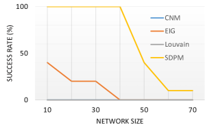
Figure 3: Success rate of finding CSs with positive modularity values in the hard instances.

VI-B  Hard Instances via Max-Cut reduction

To validate the effectiveness of modularity clustering methods, we generate hard instances of modularity clustering via the reduction from Max-Cut problem in the proof of Theorem 2. The advantages of this type of test includes: 1) Generated networks are small but yet challenging to solve and 2) Optimal solutions and objective (modularity) are known. This contrasts other test generators such as LFR [11] that often come with planted community structure but not (guaranteed) optimal solutions.

We generate the tests following the below steps:

• Generate a random (Erdős-Réyni) network $G$.

• Find the exact size $k$ of the Max-Cut in $G$ using the Biq Mac solver [25].

• Construct a network $G^{\prime}$ from the instance $\langle G,k\rangle$ of Max-Cut using the reduction in Theorem 2.

• Run modularity maximization methods on $G^{\prime}$. A method passes a test if it can find a community structure with a strictly positive modularity value.

We vary network sizes between 10 to 70, increasing by 10 and repeat the test five times for each network size. The number of times each method passes the test are shown in Fig 3. Our SDPM algorithm clearly has much higher success rate than the rest. It passes all the tests of size up to 40. The only method that manages to pass some of the tests is the Eigenvector-based method (EIG) [15]. EIG passes the tests of sizes 10, twice and sizes 20 and 30, once. These tests illustrates the excellent capability of the SDP rounding methods for hard-instances of the modularity clustering problem.

VII Conclusion

In this paper, we settle the question on the approximability of modularity clustering. We show that there is no (multiplicative) approximation algorithm with any factor $\rho>0$, unless P = NP. However, we show that there is an additive approximation algorithm that find community structure with modularity at least $\kappa Q_{OPT}-(1-\kappa)$ with $\kappa=0.766$. Not only modularity is hard to approximate, but also it is a poor indicator for the existing of community structure. The existing of high modularity clusters neither indicates the existing of community structure nor how easy it is to detect such a structure if it exists.

In the future, it is interesting to investigate additive approximation algorithms for modularity clustering, i.e., algorithms to find CS with modularity at least $Q_{OPT}-c$ for $c>0$. We conjecture that there exists $c>0$ that approximating modularity clustering within an additive approximation factor $c$ is NP-hard.

VIII Acknowledgement

This work is partially supported by NSF CAREER 0953284 and NSF CCF 1422116.

References

- [1] D. J. Watts and S. H. Strogatz, “Collective dynamics of ’small-world’ networks,” Nature, vol. 393, 1998.
- [2] M. Girvan and M. E. Newman, “Community structure in social and biological networks.” PNAS, vol. 99, no. 12, 2002.
- [3] S. Fortunato and C. Castellano, “Community structure in graphs,” Ency. of Complexity and Sys. Sci., 2008.
- [4] S. Fortunato and M. Barthelemy, “Resolution limit in community detection,” Proceedings of the National Academy of Sciences, vol. 104, no. 1, 2007.
- [5] B. H. Good, Y.-A. de Montjoye, and A. Clauset, “Performance of modularity maximization in practical contexts,” Phys. Rev. E, vol. 81, p. 046106, Apr 2010.
- [6] J. Ruan, “A fully automated method for discovering community structures in high dimensional data,” in Proc. of the IEEE Int. Conf. on Data Mining (ICDM), 2009, pp. 968–973.
- [7] P. Shakarian, P. Roos, D. Callahan, and C. Kirk, “Mining for geographically disperse communities in social networks by leveraging distance modularity,” in Proc. of the ACM Int. Conf. on Knowledge Discovery and Data Mining (KDD), 2013, pp. 1402–1409.
- [8] U. Brandes, D. Delling, M. Gaertler, R. Gorke, M. Hoefer, Z. Nikoloski, and D. Wagner, “On modularity clustering,” Knowledge and Data Engineering, IEEE Transactions on, vol. 20, no. 2, 2008.
- [9] T. N. Dinh and M. T. Thai, “Toward optimal community detection: From trees to general weighted networks,” Internet Mathematics, vol. 11, no. 3, pp. 181–200, 2015.
- [10] B. Dasgupta and D. Desai, “On the complexity of newman’s community finding approach for biological and social networks,” J. Comput. Syst. Sci., vol. 79, no. 1, pp. 50–67, Feb. 2013.
- [11] A. Lancichinetti and S. Fortunato, “Community detection algorithms: A comparative analysis,” Phys. Rev. E, vol. 80, p. 056117, Nov 2009.
- [12] V. D. Blondel, J.-L. Guillaume, R. Lambiotte, and E. Lefebvre, “Fast unfolding of communities in large networks,” Journal of Statistical Mechanics: Theory and Experiment, vol. 2008, no. 10, 2008.
- [13] T. N. Dinh and M. T. Thai, “Community detection in scale-free networks: Approximation algorithms for maximizing modularity,” in IEEE Journal on Selected Areas in Communications, 2013.
- [14] T. N. Dinh, N. P. Nguyen, and M. T. Thai, “An adaptive approximation algorithm for community detection in dynamic scale-free networks,” in Proceedings IEEE INFOCOM, 2013, pp. 55–59.
- [15] M. E. J. Newman, “Modularity and community structure in networks,” Proceedings of the National Academy of Sciences, vol. 103, 2006.
- [16] S. Arora and B. Barak, Computational Complexity: A Modern Approach, 1st ed. New York, NY, USA: Cambridge University Press, 2009.
- [17] M. R. Garey and D. S. Johnson, Computers and Intractability: A Guide to the Theory of NP-Completeness. New York, NY, USA: W. H. Freeman & Co., 1990.
- [18] D. W. Matula and F. Shahrokhi, “Sparsest cuts and bottlenecks in graphs,” Discrete Applied Mathematics, vol. 27, no. 1 2, pp. 113 – 123, 1990.
- [19] P. Vitanyi, “How well can a graph be n-colored?” Discrete mathematics, vol. 34, no. 1, pp. 69–80, 1981.
- [20] M. Charikar, V. Guruswami, and A. Wirth, “Clustering with qualitative information,” Learning Theory, J. of Comput. Syst. Sci., vol. 71, no. 3, pp. 360 – 383, 2005.
- [21] G. Agarwal and D. Kempe, “Modularity-maximizing graph communities via mathematical programming,” Eur. Phys. J. B, vol. 66, 2008.
- [22] D. Aloise, S. Cafieri, G. Caporossi, P. Hansen, S. Perron, and L. Liberti, “Column generation algorithms for exact modularity maximization in networks.” Phys. Rev. E, vol. 82, 2010.
- [23] R. H. Tütüncü, K. C. Toh, and M. J. Todd, “Solving semidefinite-quadratic-linear programs using SDPT3,” Mathematical Programming, vol. 95, no. 2, pp. 189–217, 2003.
- [24] A. Clauset, M. E. J. Newman, and C. Moore, “Finding community structure in very large networks,” Phys. Rev. E, vol. 70, p. 066111, Dec 2004.
- [25] F. Rendl, G. Rinaldi, and A. Wiegele, “Solving Max-Cut to optimality by intersecting semidefinite and polyhedral relaxations,” Math. Programming, vol. 121, no. 2, p. 307, 2010.