Abstract

The low energy limit of the stress tensor, gauge current, and supercurrent two-point correlators are calculated in the background of the supersymmetric magnetic brane solution to gauged five-dimensional supergravity constructed by Almuhairi and Polchinski. The resulting correlators provide evidence for the emergence of an ${\cal N}=2$ super-Virasoro algebra of right-movers, in addition to a bosonic Virasoro algebra and a $U(1)\oplus U(1)$-current algebra of left-movers (or the parity transform of left- and right-movers depending on the sign of the magnetic field), in the holographically dual strongly interacting two-dimensional effective field theory of the lowest Landau level.

1 Introduction

Holography provides a powerful method for the study of strongly interacting gauge theories with fermionic matter. It allows for a geometric interpretation of renormalization group (RG) flow in the dual gravity theory in terms of motion along a holographic coordinate. The dual geometry of a UV fixed point in the gauge theory is asymptotic to an $AdS$ space-time, while that of an IR fixed point is asymptotic to another $AdS$. The dimensions of the UV and IR asymptotic $AdS$ geometries need not be the same, and often differ from one another in concrete solutions. For reviews on holographic methods, see for example [1, 2, 3, 4].

The case of four-dimensional ${\cal N}=4$ supersymmetric Yang-Mills in the presence of an external magnetic field provides a non-trivial illustration of an RG flow between two fixed points which is physically relevant. The external magnetic field is associated with the gauging of a $U(1)$ subgroup of the $SU(4)$ R-symmetry group of ${\cal N}=4$ super Yang-Mills, and couples to the scalars and gauginos of the theory, but not to its gauge fields. In the low energy limit, only fermions in the lowest Landau level contribute, and their dynamics is confined to the spatial dimension along the magnetic field. The IR fixed point theory thus consists of an effective two-dimensional conformal field theory (CFT) of strongly interacting fermions of the Luttinger-liquid type (see for example [5] on strongly interacting fermion systems in one spacial dimension).

The holographic dual to the above field theory set-up is a magnetic brane, which was constructed in [6] (see also [7] for a review) as a solution to minimal five-dimensional gauged supergravity. The fact that minimal five-dimensional supergravity is a consistent truncation of Type IIB supergravity was established in [8], building on earlier results in [9], and guarantees that the solutions of [6] can be lifted up to the UV completion, namely Type IIB string theory. The magnetic brane is a smooth solution which interpolates between an asymptotic $AdS_{5}$ in the UV and an asymptotic $AdS_{3}\times T^{2}$ in the IR. The torus $T^{2}$ occupies the two spatial dimensions perpendicular to the magnetic field, and may be represented by ${\mathbb{C}}/\Lambda$ for a lattice $\omega_{1}{\mathbb{Z}}+\omega_{2}{\mathbb{Z}}$ with arbitrary period $\omega_{1},\omega_{2}\in{\mathbb{C}}$. This geometric picture indeed reflects the expected dual RG flow from four-dimensional ${\cal N}=4$ super Yang-Mills to a two-dimensional CFT. The qualitatively different IR behavior which occurs in superconductors in the presence of an external magnetic field has been studied by holographic methods as well, for example, in [10, 11].

The asymptotic symmetry of $AdS_{3}$ is enhanced from the $SO(2,2)$ isometry of $AdS_{3}$ to left- and right-moving copies of the Virasoro algebra [12], characteristic of a dual two-dimensional CFT. A holographic calculation of two-point correlators of the $U(1)$ current and stress tensor in the IR reveals the presence of a single chiral current algebra as well as left-and right-moving Virasoro algebras [13]. The coordinate transformations on $AdS_{3}$ by which these Virasoro symmetries act in the IR originate in the UV from physical deformations on $AdS_{5}$ which are not pure coordinate transformations. This effect provides a holographic realization for the emergence of symmetries in the IR which were not present in the UV.

The magnetic brane solution discussed above preserves no supersymmetry, and minimal five-dimensional supergravity has no magnetic solutions that do. Correspondingly, the supersymmetry of the ${\cal N}=4$ theory is completely broken in the IR limit, as the energy levels of scalars and gauginos are split by the magnetic field. As a result, the low energy behavior is entirely in terms of fermions.

A generalization of the magnetic brane was proposed in [14] within the framework of a non-minimal gauged five-dimensional supergravity in which the gauged $SU(4)$ is truncated to its $U(1)^{3}$ Cartan subgroup [15, 16] (see also [17] for domain wall solutions in this theory). In addition to the fields of the minimal five-dimensional supergravity, this non-minimal supergravity further contains two Maxwell super-multiplets, thereby adding a pair of Maxwell gauge fields, two real scalars, and two gauginos. Embedding the magnetic field into the truncated $U(1)^{3}$ gauge group leads to a supersymmetric magnetic brane [18]. More precisely, the supersymmetric magnetic brane is actually a two-parameter family of solutions, one parameter being the magnitude of the magnetic field, the other parametrizing its embedding into $U(1)^{3}$. A smooth supersymmetric magnetic brane solution was shown to exist via numerical methods in [19] for a special choice of embedding with enhanced symmetry. To realize the corresponding low energy supersymmetry in the dual gauge theory, it suffices to turn on a suitable constant background auxiliary $D$-field in addition to the constant background magnetic field, as was shown in [18].

The supersymmetric magnetic brane solution is again asymptotic to an $AdS_{3}\times T^{2}$ space-time, and the IR fixed point of the dual theory is again a two-dimensional CFT. However, the universality classes in the IR of the duals to the supersymmetric and non-supersymmetric magnetic branes are different. The dual to the non-supersymmetric magnetic brane contains only fermions in the IR, while the dual to the supersymmetric brane contains both fermions and bosons in the IR, and exhibits supersymmetry.

In the present paper, we shall argue that the supersymmetric magnetic brane solution has an asymptotic symmetry governed by a unitary chiral ${\cal N}=2$ super Virasoro algebra for one chirality, and a purely bosonic unitary chiral Virasoro algebra plus two unitary chiral $U(1)$ current algebras for the other chirality. To do so, we shall compute the two-point functions for the stress tensor, the $U(1)^{3}$ currents, and the supercurrent in the low energy limit. In the supergravity theory, these correlators may be extracted from the perturbations of the metric, the Maxwell gauge fields, and the gravitinos and gauginos respectively. We shall solve the linearized field equations for the perturbations, and use the method of overlapping expansions to extract the correlators.

We shall then show that the functional form of these correlators is consistent with the emergence in the IR of the symmetries, including the ${\cal N}=2$ super Virasoro algebra, announced earlier in this paragraph. In addition, the overall normalizations of the identity operator in the OPE of two stress tensors, and of two supercurrents, are accessible from the calculation of the two-point correlators of these operators, and are shown to match precisely with the form required by the ${\cal N}=2$ superconfomal algebra. The corresponding calculation of the absolute normalization for two $U(1)$ currents is significantly complicated by the mixing effects of the three $U(1)$ gauge fields by the Chern-Simons term, and a derivation of the absolute normalization of the current will not be achieved here, but will be left for future work.

The calculations of these correlators generally follow the procedures used in [13] for the minimal supergravity. For the case of non-minimal supergravity of interest here, however, they become considerably more involved, especially for the correlators of the gauge currents and supercurrent. We shall take this opportunity to present the derivations of the proper normalizations of the holographically renormalized supercurrent in some detail.

1.1 Organization

The present paper is organized as follows. In Section 2 we briefly review the essentials of the non-minimal five-dimensional supergravity theory and the formalism for the holographic calculation of stress tensor and current correlators. We discuss the structure of the supersymmetric magnetic brane solutions and demonstrate their existence numerically for a wide range of parameters. In Section 3, we compute the correlators for the stress tensor in the IR limit, following closely the methods used in [13]. In Section 4 we compute the correlators for the $U(1)^{3}$ currents in the IR limit, and disentangle their chirality dependence on the embedding parameters. In Section 5 we review the formalism for the holographic calculation of the fermionic fields in supergravity, and extract the supercurrent two-point function in the IR limit. In Section 6 we discuss the emergence of the super Virasoro symmetry in the IR limit, by putting together the information gathered from the preceding correlator calculations. A brief discussion of our results and outlook to future work is presented in section 7. In Appendix A, a comprehensive overview is presented of non-minimal five-dimensional supergravity, in which we pay careful attention to the various normalizations used in the existing literature. The construction and renormalization of the holographic supercurrent for this theory is presented in detail in Appendix B. The asymptotic expansion of the Fermi fields is relegated to Appendix C.

2 Supersymmetric magnetic brane solution

In this section, we shall give a synopsis of non-minimal five-dimensional gauged supergravity [15, 16], and discuss the supersymmetric magnetic brane solutions including their symmetries and asymptotic behavior. We shall also present numerical evidence confirming the existence of the supersymmetric magnetic brane as a regular global solution interpolating between $AdS_{5}$ in the UV and $AdS_{3}\times T^{2}$ in the IR for a wide range of parameters.

2.1 Five dimensional supergravity synopsis

The starting point is the $U(1)^{3}$ truncation of gauged five-dimensional supergravity with gauge group $SU(4)$. This supergravity is a truncation of the holographic dual to ${\cal N}=4$ four-dimensional super-Yang Mills. The bosonic fields are the space-time metric $g_{MN}$ where $M,N=0,1,2,3,4$ denote Einstein indices, three Maxwell fields $A_{M}^{I}$ labelled by $I=1,2,3$, and two neutral scalars $\phi^{A}$ with coordinate index $A=1,2$. The fermionic fields are the gravitino $\psi_{M}$ and the gaugino $\lambda^{a}$ with frame index $a=1,2$, each of which is a doublet under the $SU(2)$ R-symmetry, and is subject to the symplectic-Majorana condition.

The complete supergravity action $S_{{\rm sugra}}$ will be given by,

$$S_{{\rm sugra}}={1\over 8\pi G_{5}}\int d^{5}x\sqrt{g}\Big{(}{\cal L}_{0}+{\cal L}_{2}+{\cal L}_{4}\Big{)}+S_{{\rm bndy}}+S_{\text{ct}}$$ (2.1)

Here, $G_{5}$ is Newton’s constant in five space-time dimensions, $g=-\det(g_{MN})$, while ${\cal L}_{0},{\cal L}_{2}$, ${\cal L}_{4}$ refer to those parts of the classical Lagrangian density which are homogeneous in Fermi fields of degrees zero, two, and four respectively. For the purpose of holographic calculation and renormalization the space-time of interest will ultimately be asymptotically $AdS_{5}$ and will require a regularization cut-off near the boundary of $AdS_{5}$. These holographic procedures will require the addition of a boundary term $S_{{\rm bndy}}$ and a counter-term $S_{\text{ct}}$ needed for holographic renormalization [20, 21, 22, 23, 24], which are computed in Appendix B.

2.1.1 Bosonic part

The bosonic part of the Lagrangian density is given by,

$${\cal L}_{0} = -\frac{1}{2}R_{g}-\frac{1}{4}G_{IJ}F_{MN}^{I}F^{JMN}-\frac{1}{2}{\cal G}_{AB}\partial_{M}\phi^{A}\partial^{M}\phi^{B}-\mathfrak{g}^{2}P$$ (2.2)

$$+{1\over 48}\frac{\varepsilon^{MNPQS}}{\sqrt{g}}\,C_{IJK}F_{MN}^{I}F_{PQ}^{J}A_{S}^{K}$$

Here $\varepsilon^{MNPQS}$ is the totally anti-symmetric symbol in five dimensions, $F^{I}_{MN}=\partial_{M}A_{N}^{I}-\partial_{N}A^{I}_{M}$ is the field strength of $A_{M}^{I}$, and $\mathfrak{g}$ is the gauge coupling constant. The rank three totally symmetric tensor $C_{IJK}$ is constant by $U(1)^{3}$ gauge invariance. With the above normalization in the Lagrangian, its only non-zero component is $C_{123}=1$ and permutations thereof with all other components vanishing [25]. The potential $P$ is given by,

$$P=-6\left(X_{1}+X_{2}+X_{3}\right)$$ (2.3)

while the metrics $G_{IJ}$ and ${\cal G}_{AB}$ take the form,

$$G_{IJ}=\frac{\delta_{IJ}}{2\left(X^{I}\right)^{2}}\hskip 43.36243pt{\cal G}_{AB}={1\over 2}\delta_{AB}$$ (2.4)

Both metrics are flat, a result which is special to the $U(1)^{3}$ case, as was shown in [25]. The real scalar fields $X^{I}(\phi)$ satisfy the constraint $X^{1}X^{2}X^{3}=1$. A convenient parametrization of $X^{I}$ in terms of $\phi^{A}$ (on the branch where $X^{I}>0$ for all $I=1,2,3$) is as follows,

$$X^{I}=e^{-a^{I}_{A}\phi^{A}} a_{1}^{I}=(1,1,-2)^{I}/\sqrt{6}$$ (2.5)

$$a_{2}^{I}=(1,-1,0)^{I}/\sqrt{2}$$

The field equations for the metric $g_{MN}$, the Maxwell fields $A_{M}^{I}$, and the scalars $\phi^{A}$ in the presence of vanishing Fermi fields are as follows,

$$0 = R_{MN}+G_{IJ}\left(g^{PQ}F_{MP}^{I}F_{NQ}^{J}-\frac{1}{6}g_{MN}F_{PQ}^{I}F^{JPQ}\right)+\frac{1}{2}\delta_{AB}\partial_{M}\phi^{A}\partial_{N}\phi^{B}+\frac{2}{3}\mathfrak{g}^{2}g_{MN}P$$

$$0 = \partial_{M}\left(\sqrt{g}\,G_{IJ}F^{JMS}\right)+{1\over 16}\varepsilon^{MNPQS}C_{IJK}F_{MN}^{J}F_{PQ}^{K}$$

$$0 = \delta_{AB}\Delta_{g}\phi^{B}+12\,\mathfrak{g}^{2}a_{A}^{I}X_{I}-\frac{9}{4}\sum_{I=1}^{3}F_{MN}^{I}F^{IMN}\partial_{A}\left(X_{I}\right)^{2}$$ (2.6)

where $\partial_{A}$ are the partial derivative with respect to $\phi^{A}$, $a_{A}^{I}$ are given in (2.5), and $\Delta_{g}$ is the scalar Laplacian for the space-time metric $g_{\mu\nu}$ defined by $\Delta_{g}\phi=\sqrt{g^{-1}}\,\partial_{M}(\sqrt{g}g^{MN}\partial_{N}\phi)$.

2.1.2 Fermionic part

The Lagrangian densities ${\cal L}_{2}$ and ${\cal L}_{4}$ were derived in [16]. The terms bilinear in the fermions $\psi_{M}$ and $\lambda^{a}$ have been collected in ${\cal L}_{2}$ and are reviewed in (A.20) of Appendix A, while ${\cal L}_{4}$ will not be needed for the calculations of the correlators, and will not be presented here.

The fermion field equations, to linear order in $\psi_{M}$ and $\lambda^{a}$, may be found in (A.27) and (A.28), where the $SU(2)$ R-symmetry doublets $\psi_{M}$ and $\lambda^{a}$ have been decomposed into pairs of single-component Dirac spinors $\psi_{M\pm}$ and $\lambda^{a}_{\pm}$. The field equations for the $+$ components of the gravitino $\psi_{M}=\psi_{M+}$ and of the gaugino $\lambda^{a}=\lambda^{a}_{+}$ are given by,

$$\Psi^{M}=\Lambda^{a}=0$$ (2.7)

where we have defined,

$$\Psi^{M} = \Gamma^{MNP}\mathcal{D}_{N}\psi_{P}+\frac{3i}{8}X_{I}\left(\Gamma^{MNPR}\psi_{N}F_{PR}^{I}+2\psi_{N}F^{I\hskip 1.0ptMN}\right)-\frac{i}{2}\Gamma^{N}\Gamma^{M}\lambda^{a}f_{A}^{a}\partial_{N}\phi^{A}$$

$$-\frac{1}{4}\sqrt{\frac{3}{2}}X_{I}^{a}\Gamma^{NP}\Gamma^{M}\lambda^{a}F_{NP}^{I}+\frac{3}{2}\mathfrak{g}\,\Gamma^{MN}\psi_{N}V_{I}X^{I}-\frac{3i}{\sqrt{6}}\mathfrak{g}\,\Gamma^{M}\lambda^{a}V_{I}X^{Ia}$$

$$\Lambda^{a} = \Gamma^{M}\mathcal{D}_{M}\lambda^{a}+\frac{i}{2}\Gamma^{M}\Gamma^{N}\psi_{M}f_{A}^{a}\partial_{N}\phi^{A}-\frac{1}{4}\sqrt{\frac{3}{2}}X_{I}^{a}\Gamma^{M}\Gamma^{NP}\psi_{M}F_{NP}^{I}$$ (2.8)

$$-\frac{i}{2}\left(\frac{1}{4}\delta^{ab}X_{I}+T^{abc}X_{I}^{c}\right)\Gamma^{MN}\lambda^{b}F_{MN}^{I}-\frac{3i}{\sqrt{6}}\mathfrak{g}\,\Gamma^{M}\psi_{M}V_{I}X^{Ia}-\frac{1}{\sqrt{6}}\mathfrak{g}\,\lambda^{b}P^{ab}\hskip 36.135pt$$

The corresponding equations for the components $\psi_{M-}$ and $\lambda^{a}_{-}$ of the $SU(2)$ doublets are given by equations (2.7) and (2.1.2) with the sign of $\mathfrak{g}$ reversed $\mathfrak{g}\to-\mathfrak{g}$. The covariant derivative ${\cal D}_{M}$ in (2.1.2) is defined in (A.10) and (A.11) of Appendix A, while the frame $f_{A}^{a}$, the variables $X^{Ia}$, and the tensor $P^{ab}$ are defined respectively in (A.31), (A.5), and (A.23).

2.1.3 Supersymmetry transformations and the BPS equations

The supersymmetry transformations, to lowest order in the Fermi fields, are as follows,

$$\delta\psi_{M} = \left({\cal D}_{M}+\frac{i}{8}X_{I}F_{NP}^{I}\left(\Gamma_{M}{}^{NP}-4\delta_{M}{}^{N}\Gamma^{P}\right)-\frac{1}{2}\mathfrak{g}\,V_{I}X^{I}\Gamma_{M}\right)\epsilon$$

$$\delta\lambda_{A} = \left(-\frac{i}{2}{\cal G}_{AB}\Gamma^{M}\partial_{M}\phi^{B}+\frac{3}{8}\partial_{A}X_{I}F_{MN}^{I}\Gamma^{MN}-\frac{3i}{2}\mathfrak{g}\,V_{I}\partial_{A}X^{I}\right)\epsilon$$ (2.9)

Here $V_{I}$ is a constant vector which governs the $U(1)$ gauging specified in (A.9). We are exhibiting the supersymmetry transformation on $\lambda_{A}=f_{A}^{a}\lambda^{a}$ in (2.9) rather than on $\lambda^{a}$ in order to match the notations of [14, 17]. The full supersymmetry transformations, including all orders in the Fermi fields, were derived in [16].

The action $S_{{\rm sugra}}$ is invariant under the supersymmetry transformations (2.9) on the fermions, along with the supersymmetry transformations on the Bose fields (which we are not exhibiting here as we do not need them), provided variations trilinear in the Fermi fields $\psi_{M}$ and $\lambda^{a}$ are neglected. The Fermi field equations to linear order in the Fermi fields (2.1.2) are, however, invariant under (2.9) to leading order in the Fermi fields without transforming the Bose fields.

The BPS equations are obtained by enforcing the conditions,

$$\delta\psi_{M}=\delta\lambda^{a}=0$$ (2.10)

on a configuration with vanishing Fermi fields. A bosonic field configuration is referred to as being BPS provided the BPS equations (2.10) admit a non-zero supersymmetry transformation $\epsilon$ subject to mild asymptotic conditions on $\epsilon$.

2.2 Holographic asymptotics, stress tensor, current correlators

The maximally symmetric solution to the field equations for this non-minimal gauged supergravity is $AdS_{5}$ space-time obtained by setting $A_{M}^{I}=\phi^{A}=0$. The only remaining non-trivial equation is then $R_{MN}=4\mathfrak{g}^{2}\,g_{MN}$ whose maximally symmetric solution is an $AdS_{5}$ with radius $1/|\mathfrak{g}|$. $AdS_{5}$ admits the maximal number of 8 real supersymmetries.

We shall seek solutions which are asymptotically $AdS_{5}$ in the sense that they satisfy the Fefferman-Graham expansion. We shall choose the corresponding holographic coordinate $r=x^{4}$ and use the decomposition $x^{M}=(x^{\mu},r)$ with $\mu=0,1,2,3$ the four-dimensional Einstein index. The asymptotic $AdS_{5}$ is chosen to be located at $r=+\infty$. In these Fefferman-Graham coordinates, the metric admits the following expansion,

$$ds^{2} = dr^{2}+g_{\mu\nu}\left(x,r\right)dx^{\mu}dx^{\nu}$$

$$g_{\mu\nu}\left(x,r\right) = e^{2r}g_{\mu\nu}^{\left(0\right)}(x)+g_{\mu\nu}^{\left(2\right)}\left(x\right)+e^{-2r}g_{\mu\nu}^{\left(4\right)}(x)+re^{-2r}g_{\mu\nu}^{\left(\ln\right)}\left(x\right)+{\cal O}(e^{-4r})$$ (2.11)

while the asymptotic expansions for the gauge fields and scalars are given by,

$$A_{\mu}^{I}(x,r) = A_{\mu}^{I\,(0)}(x)+e^{-2r}A_{\mu}^{I\,(2)}(x)+{\cal O}(e^{-4r})$$

$$\phi^{A}(x,r) = \phi^{A\,(0)}(x)+e^{-2r}\phi^{A\,(2)}(x)+r\,e^{-2r}\phi^{A\,({\rm ln})}(x)+{\cal O}(e^{-4r})$$ (2.12)

Here, $x$ stands for the dependence on $x^{\mu}$, while Fefferman-Graham gauge is governed by $g_{\mu r}=g_{r\mu}=0$, $g_{rr}=1$, and $A_{r}=0$. The holographic source fields are $g^{(0)}_{\mu\nu}$, $A_{\mu}^{I\,(0)}$ and $\phi^{A\,(0)}$. Use of the field equations in (2.1.1) shows that the coefficients $g_{\mu\nu}^{(2)}$, $g_{\mu\nu}^{(\ln)}$, the trace of $g_{\mu\nu}^{(4)}$, and $\phi^{A\,({\rm ln})}$ are local functionals of $g_{\mu\nu}^{(0)}$, $A_{\mu}^{I\,(0)}$ and $\phi^{A\,(0)}$.

The response of the action $S_{{\rm sugra}}$ to infinitesimal variations of the source fields is given by the expectation values of the dual operators in the field theory [20, 21, 22, 23, 24]. In the present case, the response to the variation of the source fields $g_{\mu\nu}^{(0)}$, $A_{\mu}^{I(0)}$, and $\phi^{A(0)}$ is given by the expectation values $T^{\mu\nu}$, $J^{\mu}_{I}$ and $Y_{A}$ respectively of the stress tensor ${\cal T}^{\mu\nu}$, the gauge current ${\cal J}^{\mu}_{I}$, and scalar operator ${\cal Y}_{A}$,

$$\delta S_{{\rm sugra}}=\int d^{4}x\sqrt{g^{(0)}}\left(\frac{1}{2}T^{\mu\nu}\,\delta g_{\mu\nu}^{(0)}+J^{\mu}_{I}\,\delta A_{\mu}^{I\,(0)}+Y_{A}\,\delta\phi^{A\,(0)}\right)$$ (2.13)

The expectation values are given in terms of the boundary field data by,

$$4\pi G_{5}T_{\mu\nu} = g_{\mu\nu}^{\left(4\right)}+\rm{local}$$

$$4\pi G_{5}J_{\mu}^{I}\leavevmode\nobreak\ = A_{\mu}^{I\,(2)}+\rm{local}$$

$$2\pi G_{5}Y^{A} = \phi^{A\,(2)}+{\rm local}$$ (2.14)

The indices $\mu,\nu$ are lowered with the help of $g_{\mu\nu}^{(0)}$, while the indices $I$ and $A$ are lowered respectively with the help of the metrics $G_{IJ}(\phi)$ and ${\cal G}_{AB}(\phi)=\delta_{AB}/2$ evaluated at the fields $\phi^{A\,(0)}$. In equations (2.2) the “local” terms refers to local functionals of $g_{\mu\nu}^{\left(0\right)}$, $A_{\mu}^{I\,(0)}$, and $\phi^{A\,(0)}$ which will not contribute to two-point functions of local operators evaluated at distinct points, and will not be retained further.

The Fefferman-Graham expansion for the fermion fields $\psi_{M}$ and $\lambda^{a}$ will involve more formalism and will be presented in Section 5.

2.3 The supersymmetric magnetic brane solution

The magnetic brane solutions considered here are holographic duals to ${\cal N}=4$ four-dimensional supersymmetric Yang-Mills theory in the presence of a constant uniform external magnetic field. The magnetic field is taken to be in the $1$-direction, perpendicular to the $23$-plane. The symmetries of this set-up are translation invariance along the four physical space-time directions $x^{\mu}$ with $\mu=0,1,2,3$, Lorentz invariance in the $01$-plane, and rotation invariance in the $23$-plane. The most general Ansatz, for the bosonic fields, which is consistent with these symmetries in this supergravity theory is given as follows,

$$ds^{2} = dr^{2}+e^{2W(r)}\eta_{mn}dx^{m}dx^{n}+e^{2U(r)}\delta_{ij}dx^{i}dx^{j}$$

$$F^{I} = F_{23}^{I}\,dx^{2}\wedge dx^{3}$$

$$\phi^{A} = \phi^{A}(r)$$ (2.15)

where $\eta={\rm diag}(-1,+1)$ is the flat Minkowski metric in the $01$-plane while $\delta_{ij}$ is the flat Euclidean metric in the $23$-plane, with $m,n=0,1$ and $i,j=2,3$. It will often be convenient to parametrize the $01$-plane by light-cone coordinates $x^{\pm}$ and the $23$-plane by complex coordinates $x^{u}$ and $x^{v}=(x^{u})^{*}$ defined as follows,

$$\eta_{mn}dx^{m}dx^{n}=2dx^{+}dx^{-} x^{\pm}=(\pm x^{0}+x^{1})/\sqrt{2}$$

$$\delta_{ij}dx^{i}dx^{j}=2dx^{u}dx^{v}\leavevmode\nobreak\ x^{u}\,=(x^{2}+ix^{3})/\sqrt{2}$$ (2.16)

The functions $U,W,\phi^{A}$ depend only on $r$ in view of translation invariance in $x^{\mu}$, while the field strength components $F_{23}^{I}$ are constant in view of the Bianchi identities. The constants $F^{I}_{23}$ may be parametrized by the magnitude of a magnetic field $B>0$ and a vector of charges $q^{I}$ which specifies the embedding of the magnetic field in $U(1)^{3}$ by setting,

$$F_{23}^{I}=q^{I}B$$ (2.17)

This parametrization is not unique, as $B$ and $q^{I}$ may be rescaled while leaving their product fixed. We shall shortly impose a normalization on $q^{I}$ to eliminate this arbitrariness. Translation invariance of the Ansatz in the 23 directions allows us to consider solutions in which the topology of the 23-space is either flat ${\mathbb{R}}^{2}$ or a compactification of ${\mathbb{R}}^{2}$ to a flat torus $T^{2}$ which may be represented in ${\mathbb{R}}^{2}={\mathbb{C}}$ as the quotient ${\mathbb{C}}/\Lambda$ by a lattice $\omega_{1}{\mathbb{Z}}+\omega_{2}{\mathbb{Z}}$ with arbitrary period $\omega_{1},\omega_{2}\in{\mathbb{C}}$.

Minimal five-dimensional supergravity may be obtained from non-minimal supergravity by setting $A^{I}_{M}=A_{M}$ for $I=1,2,3$, which amounts to setting all charges $q^{I}$ equal to one another. The scalars may then be set to zero, $\phi^{A}=0$, so that $X^{I}=1$, which allows us to set the gaugino to zero $\lambda^{a}=0$. The magnetic brane solution constructed in [6] for this minimal five-dimensional Einstein-Maxwell-Chern-Simons theory breaks all supersymmetries.

Supersymmetric magnetic brane solutions exist if and only if the relation $q^{1}+q^{2}+q^{3}=0$ holds and $V_{I}$ satisfies $V_{I}q^{I}=0$. We shall set,

$$V_{I}={1\over 3}\hskip 36.135ptI=1,2,3$$ (2.18)

This condition forces the composite $U(1)$-gauge field ${\cal A}_{M}$ to vanish on the solution so that the covariant derivative ${\cal D}_{M}$ on a spinor $\epsilon$ reduces to the covariant derivative with the spin connection $\omega_{M}$ given by (A.11), and takes the following form on the Ansatz (2.15),

$$dx^{M}{\cal D}_{M}\epsilon=d\epsilon-{1\over 2}dx^{m}W^{\prime}\,\Gamma^{r}\Gamma_{m}\epsilon-{1\over 2}dx^{i}U^{\prime}\,\Gamma^{r}\Gamma_{i}\epsilon$$ (2.19)

where ^′ denotes differentiation in $r$.

2.3.1 The reduced BPS equations

The supersymmetric magnetic brane solution proposed in [14, 18], and further investigated in [19], is a solution to the BPS equations (2.9) and (2.10) reduced to the Ansatz of (2.15). These reduced BPS equations are invariant under Lorentz transformations in the $01$-plane and rotations in the $23$-plane respectively generated by,

$$\Gamma^{{\hat{+}}{\hat{-}}} = \Gamma^{\hat{0}\hat{1}}\hskip 16.62178pt=\Gamma^{+}{}_{+}\hskip 7.22743pt=-\Gamma^{-}{}_{-}$$

$$\Gamma^{{\hat{u}}{\hat{v}}}\, = -i\Gamma^{\hat{2}\hat{3}}\leavevmode\nobreak\ =-i\Gamma^{2}{}_{3}=i\Gamma^{3}{}_{2}$$ (2.20)

The generators $\Gamma^{{\hat{+}}{\hat{-}}}$ and $\Gamma^{{\hat{u}}{\hat{v}}}$ square to unity, mutually commute, and commute with $\Gamma^{\hat{r}}=\Gamma^{r}$. Their product $\Gamma^{{\hat{+}}{\hat{-}}}\Gamma^{{\hat{u}}{\hat{v}}}\Gamma^{\hat{r}}=-i\Gamma^{\hat{0}\hat{1}\hat{2}\hat{3}\hat{4}}$ equals $\pm I$. The two possible signs distinguish the two irreducible representations of the Clifford algebra in odd dimensions which, however, lead to equivalent representations of the Lorentz group, mapped into one another by parity. Using the convention adopted in Section A.1, we choose,

$$\Gamma^{{\hat{+}}{\hat{-}}}\,\Gamma^{{\hat{u}}{\hat{v}}}\,\Gamma^{\hat{r}}=I$$ (2.21)

The BPS equations may be separated by simultaneously diagonalizing $\Gamma^{\hat{r}}$ and $\Gamma^{{\hat{u}}{\hat{v}}}$,

$$\Gamma^{{\hat{r}}}\,\epsilon=\gamma\,\epsilon\hskip 72.26999pt\Gamma^{{\hat{u}}{\hat{v}}}\,\epsilon=-\eta\,\gamma\,\epsilon$$ (2.22)

where $\gamma$ and $\eta$ are independent from one another and may take the values $\pm 1$.

The reduced BPS equation for the index $M=r$ is a differential equation for $\epsilon$ which we shall not need here. Assuming the existence of a non-vanishing spinor $\epsilon$, the reduced BPS equations of (2.10) for $M=\mu=0,1,2,3$ are algebraic and given by,

$$0 = W^{\prime}-\mathfrak{g}\,\gamma V_{I}X^{I}+\frac{1}{2}\eta\,B\,q^{I}X_{I}\,e^{-2U}$$

$$0 = U^{\prime}-\mathfrak{g}\,\gamma V_{I}X^{I}-\eta\,B\,q^{I}X_{I}\,e^{-2U}$$

$$0 = \delta_{AB}(\phi^{B})^{\prime}+6\mathfrak{g}\,\gamma V_{I}\partial_{A}X^{I}+3\eta\,B\,q^{I}\partial_{A}X_{I}\,e^{-2U}$$ (2.23)

The magnitude of $\mathfrak{g}$ may be scaled to 1 by rescaling $B$ and $r$. The eigenvalue $\gamma$ is correlated with the sign of $\mathfrak{g}$. To see this, note that the supersymmetric magnetic brane solution should reduce to the $AdS_{5}$ solution upon letting $B\to 0$. For this solution to exist, given that we have chosen the branch $X^{I}>0$ in (2.5), along with (2.18), we must have,

$$\gamma=\mathfrak{g}$$ (2.24)

Having set $\gamma=\mathfrak{g}$ for $|\mathfrak{g}|=1$, the BPS equations are independent of the sign of $\mathfrak{g}$. Similarly, the eigenvalue $\eta$ is given as follows,

$$\eta={\rm sign}(q^{1}q^{2}q^{3})$$ (2.25)

a relation which is required in order to have a solution asymptotic to $AdS_{3}\times T^{2}$.

2.3.2 The $AdS_{3}\times T^{2}$ solution

The reduced BPS equations, with a supersymmetric charge arrangement $q^{1}+q^{2}+q^{3}=0$ and none of the charges $q^{I}$ vanishing, admit an exact $AdS_{3}\times T^{2}$ solution [14] given by,

$$W=\frac{r}{L}\hskip 50.58878pte^{2U}=\bar{q}\,B\hskip 50.58878ptX^{I}={\left(q^{I}\right)^{2}\over 4\bar{q}^{2}}\hskip 50.58878ptF_{23}^{I}=q^{I}B$$ (2.26)

Recall our choice $B>0$, and the charges $q^{I}$ characterizing the embedding of the magnetic field in the $U(1)^{3}$ gauge group. The $AdS_{3}$ radius $L$ and the combination $\bar{q}$ are given by,

$${1\over L}=\frac{3}{2}V_{I}X^{I}\hskip 72.26999pt\bar{q}={1\over 2}|q^{1}q^{2}q^{3}|^{{1\over 3}}$$ (2.27)

The above $AdS_{3}\times T^{2}$ solution is regular, and preserves one of the four symplectic Majorana supersymmetries. When one of the charges $q^{I}$ vanishes, the number of supersymmetry generators is doubled but, as is clear from the above expressions, there is no regular solution with an asymptotic $AdS_{3}\times T^{2}$ behavior in the IR. Henceforth, we shall assume that none of the charges vanishes and, by suitably rescaling $B$, we shall choose,

$$\bar{q}=1$$ (2.28)

As a function of the three real charges $q^{I}$, subject to the condition $V_{I}q^{I}=0$, one readily establishes the allowed range of the $AdS_{3}$ radius $L$, which is $0<L<L_{0}$ with $L_{0}=2^{2/3}/3$. The maximum value $L_{0}$ is uniquely attained when any two of the charges $q^{I}$ coincide.

2.3.3 Asymptotic $AdS_{3}\times T^{2}$ behavior of the supersymmetric magnetic brane

The supersymmetric magnetic brane solution, for given magnetic field $B$ and embedding charges $q^{I}$, has $F_{23}^{I}=Bq^{I}$ and the leading asymptotics for its remaining fields coincide with the exact $AdS_{3}\times T^{2}$ solution given in the preceding subsection. The detailed $r\rightarrow-\infty$ asymptotics near $AdS_{3}\times T^{2}$, including the leading deviation away from the exact solution of (2.26), is found to be given as follows,

$$W\left(r\right) = \frac{r}{L}+\frac{1}{\sigma}\left(2V_{I}\partial_{A}X_{(0)}^{I}c^{A}-\frac{2}{3L}c^{0}\right)e^{\sigma r}+\mathcal{O}\left(e^{2\sigma r}\right)$$

$$U\left(r\right) = \frac{1}{2}\ln B+c^{0}\,e^{\sigma r}+\mathcal{O}\left(e^{2\sigma r}\right)$$

$$\phi^{1}\left(r\right) = -\sqrt{6}\ln\left(q^{1}q^{2}\right)+c^{1}\,e^{\sigma r}+\mathcal{O}\left(e^{2\sigma r}\right)$$

$$\phi^{2}\left(r\right) = -\sqrt{2}\ln\left({q^{1}\over q^{2}}\right)+c^{2}\,e^{\sigma r}+\mathcal{O}\left(e^{2\sigma r}\right)$$ (2.29)

The coefficients $c^{0},c^{1},c^{2}$ are components of an eigenvector, associated with eigenvalue $\sigma$, of a symmetric matrix $\mathfrak{S}$. Explicitly, these relations are given by,

$$\mathfrak{S}\left(\begin{matrix}c^{0}\cr c^{A}\end{matrix}\right)=\sigma\left(\begin{matrix}c^{0}\cr c^{A}\cr\end{matrix}\right)$$ (2.30)

where the indices $A,B$ take the values $1,2$, and $\mathfrak{S}$ is given by,

$$\mathfrak{S}^{00}\,\, = \frac{4}{3L}$$

$$\mathfrak{S}^{0A}\, = -V_{I}\partial_{A}X^{I}$$

$$\mathfrak{S}^{AB} = -6V_{I}\partial_{A}\partial_{B}X^{I}-3\eta Bq^{I}\partial_{A}\partial_{B}X_{I}e^{-2U}$$ (2.31)

Here, it is understood that the fields $X^{I}$ and $U$ are evaluated on the $AdS_{3}$ solution of (2.26), which is exclusively in terms of the charges $q^{I}$. Since $\mathfrak{S}$ is a symmetric matrix, its eigenvalues $\sigma$ are guaranteed to be real and they solve the characteristic equation,

$$\sigma^{3}-\frac{4}{L^{2}}\sigma+16=0$$ (2.32)

For $0<L<1/\sqrt{3}$, the three roots are real, two being positive and one negative. The root chosen here is always the largest positive root. At $L=1/\sqrt{3}$, we have $\sigma=2$, and for $L<1/\sqrt{3}$ the value of $\sigma$ monotonically increases with decreasing positive $\sigma$, reaching the asymptotic expression $\sigma\approx 2/L$ as $L\to 0$. The range $0<L<L_{0}=2^{2/3}/3$ established earlier for $L$ is strictly contained in this interval since $L_{0}<1/\sqrt{3}$, so that the two positive roots never become degenerate for $0<L<L_{0}$, and the largest root always satisfies $\sigma>2$.

The overall magnitude of the vector $(c^{0},c^{1},c^{2})$ is not fixed by the local asymptotic expansion, but may be related, by numerical integration of the full supersymmetric magnetic brane solution which interpolates between $AdS_{3}\times T^{2}$ and $AdS_{5}$, to the asymptotic behavior near $AdS_{5}$, to be given below.

2.3.4 Asymptotic $AdS_{5}$ behavior of the supersymmetric magnetic brane

Given the magnetic field $B$ and the embedding charges $q^{I}$, as well as the $AdS_{3}\times T^{2}$ asymptotics of the solution spelled out in the preceding subsection, the $r\rightarrow\infty$ asymptotics of the metric fields $U,W$ are as follows,

$$W\left(r\right) = r+\ln W_{0}+{\cal O}\left(e^{-4r}\right)$$

$$U\left(r\right) = r+\ln U_{0}+{\cal O}\left(e^{-4r}\right)$$ (2.33)

The constants $W_{0}$ and $U_{0}$ are functions of the magnetic field $B$, the charges $q^{I}$, and the overall magnitude of the coefficient vector $c^{0},c^{1},c^{2}$ in the $AdS_{3}\times T^{2}$ asymptotics, and can be read off from the numerical solution, where the metric at $r\rightarrow\infty$ takes the form,

$$ds^{2}=dr^{2}+W_{0}^{2}\,e^{2r}\eta_{mn}dx^{m}dx^{n}+U_{0}^{2}\,e^{2r}\delta_{ij}dx^{i}dx^{j}$$ (2.34)

The physical meaning of the constants $W_{0}$ and $U_{0}$ is to provide the constant rescaling factors between the coordinates of space-time $x^{m},x^{i}$ between the IR region for $r\to-\infty$ and the UV region for $r\to+\infty$. Naturally, one could rescale the coordinates $x^{m}$ by $W_{0}$ and $x^{i}$ by $U_{0}$ to recover standard normalizations in the $AdS_{5}$ region, at the expense of rescaling the coordinates also in the $AdS_{3}\times T^{2}$ region. The present choice of normalization will be the more convenient one for our purpose.

The leading asymptotic behavior of the scalar fields $\phi^{A}$ is given by (2.26) and the second line in (2.12). Its sub-leading asymptotics will not be presented here, as it will not be needed in the sequel. The coefficients $g^{(4)}_{\mu\nu}$ and $\phi^{A\,(2)}$ are not determined by the local expansion, but may again be determined by numerically integrating the field equations.

2.3.5 Global regular solutions obtained numerically

The existence of a regular solution to the reduced BPS equations of (2.3.1) for the charge assignment $q^{1}=q^{2}$ was shown numerically in [19]. We shall supplement this result by exhibiting regular solutions to (2.3.1) which interpolate between $AdS_{3}\times T^{2}$ and $AdS_{5}$ over a range of charge assignments, again by numerical integration. Without loss of generality, we permute the $q^{I}$ so that $q^{1}$ and $q^{2}$ have the same sign and $q^{2}<q^{1}$. We introduce a single parameter $\alpha$ to characterize the solution, as follows,

$$\alpha={q^{2}\over q^{1}}\hskip 72.26999pt0<\alpha<1\hskip 36.135pt{\rm sign}(q^{3})=\eta$$ (2.35)

where $\eta$ is the sign factor introduced in (2.25).

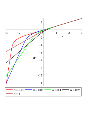
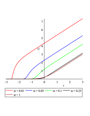
Figure 1: The $r$-dependence of the metric functions $U$ and $W$, obtained numerically for $\alpha=1,\,0.25,\,0.1,\,0.05$, and $0.01$.

Figure 2: The $r$-dependence of the scalar functions $X^{1}$ and $X^{2}$, obtained numerically for $\alpha=1,\,0.25,\,0.1,\,0.05$, and $0.01$.

The corresponding asymptotics of the metric as $r\to\infty$ is given by (2.34) and $X^{I}\to 1$, while the asymptotics as $r\to-\infty$ for the metric function $U$ is constant, and is given for all functions in (2.3.3). In particular, for the scalar fields $X^{I}$, the asymptotics as $r\to-\infty$ is given by the $AdS_{3}\times T^{2}$ solution in (2.26) and we have,

$$X^{1}=\left({1\over\alpha(1+\alpha)}\right)^{2\over 3}\hskip 43.36243ptX^{2}=\left({\alpha^{2}\over 1+\alpha}\right)^{{2\over 3}}\hskip 43.36243ptX^{3}=\left({(1+\alpha)^{2}\over\alpha}\right)^{{2\over 3}}$$ (2.36)

We have verified that by using the largest positive root $\sigma$ of (2.32) in the initial conditions for the $AdS_{3}\times T^{2}$ region, there always exists a solution that matches onto $AdS_{5}$ in the UV for the following values,

$$\alpha=1,\,0.5,\,0.25,\,0.1,\,0.05,\,0.025,\,0.01,\,0.005,\,0.0025,\,0.001$$ (2.37)

of which we have depicted a subset in figures 1 and 2. The dependence on $\alpha$ from one value to another appears to be smooth.

3 Stress tensor correlators

In this section, we shall compute the two-point correlators of the components in the $01$-plane of the stress tensor in the presence of the supersymmetric magnetic brane solution, in the IR limit. We follow the method of [13] and solve the linearized Einstein equations for the corresponding components of the metric fluctuations $\delta g_{\mu\nu}$ with specified holographic boundary condition $\delta g_{\mu\nu}^{(0)}$. From this solution, we obtain the induced expectation value $T^{\mu\nu}(x)$ of the stress tensor operator ${\cal T}^{\mu\nu}(x)$ via the first equation of (2.2) and read off the correlator from the linear response formula,

$$T^{\mu\nu}(x)=\frac{i}{2}\int d^{4}y\,\sqrt{g^{(0)}}\left\langle{\cal T}^{\mu\nu}(x){\cal T}^{\rho\sigma}(y)\right\rangle\delta g_{\rho\sigma}^{(0)}(y)$$ (3.1)

We begin by isolating the fluctuations needed to calculate the desired correlators.

3.1 Structure of the perturbations

In this section we shall determine the structure of the perturbations around the supersymmetric magnetic brane solution needed to compute the two-point correlators of the components of the stress tensor and the currents in the directions of the $01$-plane.

Since the supersymmetric magnetic brane solution is invariant under translations in $x^{\mu}$ for $\mu=0,1,2,3$ a general linear perturbation is a linear combination of plane waves, each with given momentum $p_{\mu}$. Physically relevant to probing the dynamics of the effective low energy CFT in the $01$-plane is the dependence of the perturbations on the components $p_{\pm}$ only, so that we may set $p_{2}=p_{3}=0$.

Arbitrary perturbations of the metric around the supersymmetric magnetic brane will generally mix with gauge field and scalar perturbations. However, if we restrict the perturbations of the metric to the directions in the $01$-plane, namely if we turn on only the components $\delta g_{\pm\pm}$ and $\delta g_{+-}$ then it may be seen from the action that no mixing with the other components of metric fluctuations, the gauge fields, and the scalar fields will occur as long as $p_{2}=p_{3}=0$. Key ingredients in the argument are the invariances of the supersymmetric magnetic brane under translations along $x^{\mu}$ for $\mu=0,1,2,3$, Lorentz transformations in the $01$-plane, and rotations in the $23$-plane.

Consider, for example, the effect of turning on the fluctuation $\delta g^{++}=g^{+-}g^{+-}\delta g_{--}$ on the gauge kinetic energy term proportional to $G_{IJ}(\phi)g^{MN}g^{PQ}F^{I}_{MP}F^{J}_{NQ}$. Since the gauge field strength of the supersymmetric brane solution is in the direction $F^{I}_{23}$ only, a fluctuation linear in $\delta g^{++}$ can turn on neither the fluctuation $\delta F^{I}_{+-}$ nor the fluctuation $\delta F_{23}$. It can also not turn on the fluctuations of the scalar field. The arguments for the other couplings in the action are similar.

Therefore, we consider the following plane wave perturbation $h_{mn}(r,p_{\pm})e^{ip\cdot x}$ with momentum $p_{\pm}$ of the supersymmetric magnetic brane,

$$ds^{2} = ds_{B}^{2}+h_{mn}(p_{\pm},r)\,e^{ip\cdot x}\,dx^{m}dx^{n}$$

$$F^{I} = q^{I}B\,dx^{2}\wedge dx^{3}$$

$$\phi^{A} = (\phi_{B})^{A}$$ (3.2)

where $ds_{B}^{2}$ and $(\phi_{B})^{A}$ are respectively the metric and the scalar fields of the supersymmetric magnetic brane given by the Ansatz (2.15) with $U,W,(\phi_{B})^{A}$ provided by the numerical solution to (2.3.1). The indices $m,n$ take the values $0,1$ or equivalently $\pm$ and we shall use the following notations throughout for the inner product and norm in the $01$-plane,

$$p\cdot x=p_{+}x^{+}+p_{-}x^{-}\hskip 72.26999ptp^{2}=2p_{+}p_{-}$$ (3.3)

Finally, we shall be interested only in momenta which are small compared with the inverse radius $|\mathfrak{g}|$ of $AdS_{5}$, which here has been set to 1, so that we shall work in the regime,

$$0<p^{2}\ll 1$$ (3.4)

In this limit the equations for the metric perturbations $h_{\pm\pm}$ may be solved by matching the asymptotic expansion valid in the near and far regions. The near region is the range of $r$ where $AdS_{3}\times T^{2}$ is a good approximation, namely $e^{2r}\ll 1$, while the far region is the range of $r$ for which we can neglect the momenta, namely $p^{2}\ll e^{2r}$. In view of (3.4), the overlap region $p^{2}\ll e^{2r}\ll 1$ is parametrically large, and matching the solutions in the near and far regions in the overlap region will produce a linearized solution valid for all $r$.

The linearized field equations for the perturbations (3.1) of the metric are,

$$0 = 3h_{\pm\pm}^{\prime\prime}-6(W^{\prime}-U^{\prime})h_{\pm\pm}^{\prime}+12(W^{\prime})^{2}h_{\pm\pm}-\mathfrak{F}\,h_{\pm\pm}$$

$$0 = (p_{\mp}h_{\pm\pm}-p_{\pm}h_{+-})^{\prime}-2W^{\prime}(p_{\mp}h_{\pm\pm}-p_{\pm}h_{+-})$$

$$0 = 3h_{+-}^{\prime\prime}+6U^{\prime}h_{+-}^{\prime}+3e^{-2W}(p_{-}^{2}h_{++}+p_{+}^{2}h_{--}-2p_{+}p_{-}h_{+-})-\mathfrak{F}\,h_{+-}$$

$$0 = h_{+-}^{\prime\prime}-2W^{\prime}h_{+-}^{\prime}-2W^{\prime\prime}h_{+-}$$ (3.5)

Here, the prime denotes differentiation with respect to $r$, the dependence on $r$ and $p_{\pm}$ is understood, and we have introduced the following abbreviation,

$$\mathfrak{F}=B^{2}e^{-4U}\left[\left(\frac{q^{1}}{X^{1}}\right)^{2}+\left(\frac{q^{2}}{X^{2}}\right)^{2}+\left(\frac{q^{3}}{X^{3}}\right)^{2}\right]+8\left(\frac{1}{X^{1}}+\frac{1}{X^{2}}+\frac{1}{X^{3}}\right)$$ (3.6)

We shall need of this function only its asymptotic values in the $AdS_{5}$ and $AdS_{3}\times T^{2}$ regions, which evaluate to $24$ and $12/L^{2}$, respectively.

3.2 Near Region

In the near region, where $e^{2r}\ll 1$, we set the background metric equal to the metric of the $AdS_{3}\times T^{2}$ solution of (2.26) given by,

$$ds_{B}^{2}=dr^{2}+e^{\frac{2r}{L}}\eta_{mn}dx^{m}dx^{n}+B\delta_{ij}dx^{i}dx^{j}$$ (3.7)

and the scalar fields $X^{I}$ equal to the values given in (2.26). All dependence on the charges $q^{I}$ and the magnetic field $B$ is through the $AdS_{3}$ radius $L$ only. The linearized field equations derived from (3.5) in the near region are given by,

$$0 = h_{\pm\pm}^{\prime\prime}-\frac{2}{L}h_{\pm\pm}^{\prime}$$

$$0 = \left(p_{\pm}h_{+-}-p_{\mp}h_{\pm\pm}\right)^{\prime}-\frac{2}{L}\left(p_{\pm}h_{+-}-p_{\mp}h_{\pm\pm}\right)$$

$$0 = h_{+-}^{\prime\prime}-\frac{4}{L^{2}}h_{+-}+e^{-\frac{2r}{L}}\left(p_{-}^{2}h_{++}+p_{+}^{2}h_{--}-2p_{+}p_{-}h_{+-}\right)$$

$$0 = h_{+-}^{\prime\prime}-{2\over L}h_{+-}^{\prime}$$ (3.8)

where the prime denotes differentiation with respect to $r$. From the equations on the first and last lines of (3.8), it is clear that the solutions for the components $h_{\pm\pm}$ and $h_{+-}$ are all of the form,

$$h_{\mu\nu}(p_{\pm},r)=s_{\mu\nu}(p_{\pm})\,e^{\frac{2r}{L}}+t_{\mu\nu}(p_{\pm})$$ (3.9)

where the Fourier coefficients $s_{\mu\nu}$ and $t_{\mu\nu}$ depend on $p_{\pm}$, but are independent of $r$. The equations on the second and third lines in (3.8) impose the following relations between the Fourier coefficients $s_{\mu\nu}(p_{\pm})$ and $t_{\mu\nu}(p_{\pm})$,

$$t_{++}(p_{\pm}) = \frac{p_{+}}{p_{-}}\,t_{+-}(p_{\pm})$$

$$t_{--}(p_{\pm}) = \frac{p_{-}}{p_{+}}\,t_{+-}(p_{\pm})$$

$$t_{+-}(p_{\pm}) = \frac{L^{2}}{4}\Big{(}p_{-}^{2}s_{++}(p_{\pm})+p_{+}^{2}s_{--}(p_{\pm})-2p_{+}p_{-}s_{+-}(p_{\pm})\Big{)}$$ (3.10)

As is familiar from [13], we can identity the Fourier coefficients $s_{\mu\nu}$ and $t_{\mu\nu}$ as contributing to the Fourier transforms of the perturbation of the conformal boundary metric $\delta g_{\mu\nu}^{(0)}$ and the boundary stress tensor $\delta g_{\mu\nu}^{(4)}$, respectively. The top two lines of (3.10) express the linearized conservation equations of the stress tensor while the last line expresses the linearized trace anomaly of the stress tensor.

3.3 Far region

In the far region, where $p^{2}\ll e^{2r}$, we can ignore the momentum dependent terms, and we shall no longer exhibit the dependence on the momenta of the fluctuations $h_{\mu\nu}$. We will also take $h_{+-}=0$ in the far region, since this term will contribute to correlators involving $T_{+-}$ which contain only contact terms.

The linearized field equations for $h_{\pm\pm}$ with the momentum terms dropped are identical to the equations for $e^{2W}$ in the Einstein equations (2.1.1) with Ansatz (2.15). Therefore, a first solution is given by,

$$h^{1}\left(r\right)=e^{2W\left(r\right)}$$ (3.11)

where $W$ is the interpolating solution of the BPS equations. By analogy with [13], we find that another linearly independent solution is given by,

$$h^{2}(r)=e^{2W(r)}\int_{\infty}^{r}dr^{\prime}\,e^{-2W(r^{\prime})-2U(r^{\prime})}$$ (3.12)

Asymptotically, these functions have the following form. As $r\to\infty$, we have,

$$h^{1}(r)\sim e^{2r}\hskip 72.26999pth^{2}(r)\sim-{1\over 4U_{0}^{2}}\,e^{-2r}$$ (3.13)

while the asymptotics in the overlap region where $p^{2}\ll e^{2r}\ll 1$, namely as $r\to-\infty$, is given as follows,

$$h^{1}(r)\sim e^{{2r\over L}}\hskip 72.26999pth^{2}(r)\sim-{L\over 2B}$$ (3.14)

Therefore, our solution in the far region is given by the linear combination,

$$h_{\pm\pm}(r)=h^{1}(r)\,\delta g_{\pm\pm}^{(0)}-4U_{0}^{2}h^{2}(r)\,\delta g_{\pm\pm}^{(4)}$$ (3.15)

with coefficients chosen to obtain the following asymptotic form at $r\rightarrow\infty$:

$$h_{\pm\pm}(r)\sim e^{2r}\,\delta g_{\pm\pm}^{(0)}+e^{-2r}\,\delta g_{\pm\pm}^{(4)}$$ (3.16)

The $r\rightarrow-\infty$ asymptotics of (3.15) then follows, by

$$h_{\pm\pm}(r)\sim e^{\frac{2r}{L}}\,\delta g_{\pm\pm}^{(0)}+\frac{2U_{0}^{2}L}{B}\,\delta g_{\pm\pm}^{(4)}$$ (3.17)

3.4 Matching and IR Correlators

In the overlap region where $p^{2}\ll e^{2r}\ll 1$, the solutions (3.9) and (3.17) should match. Eliminating $s_{\mu\nu}$ and $t_{\mu\nu}$ between (3.9), (3.17), and (3.10) gives the following relations between $\delta g^{(0)}_{\pm\pm}$ and $\delta g^{(4)}_{\pm\pm}$,

$$\delta g_{++}^{\left(4\right)} = \frac{BL}{8U_{0}^{2}}\left(\frac{p_{+}^{3}}{p_{-}}\,\delta g_{--}^{(0)}+p_{+}p_{-}\,\delta g_{++}^{(0)}\right)$$

$$\delta g_{--}^{\left(4\right)} = \frac{BL}{8U_{0}^{2}}\left(\frac{p_{-}^{3}}{p_{+}}\,\delta g_{++}^{(0)}+p_{+}p_{-}\,\delta g_{--}^{(0)}\right)$$ (3.18)

From (2.2), the stress tensor is given by $4\pi G_{5}T_{\pm\pm}=\delta g_{\pm\pm}^{\left(4\right)}$ up to local terms. In order to normalize the stress tensor correlator to the conventional form suitable for two-dimensional CFTs, we define the two-dimensional stress tensor by $\tilde{{\cal T}}_{\pm\pm}=U_{0}^{2}V_{2}{\cal T}_{\pm\pm}$, where $V_{2}$ denotes the volume of the compactified $23$-plane. Writing $\tilde{T}_{\pm\pm}$ in terms of the Brown-Henneaux central charge of the 1+1 dimensional CFT, given by,

$$c=\frac{3L}{2G_{3}}=\frac{3LV_{2}}{2G_{5}}B$$ (3.19)

we obtain,

$$\tilde{T}_{\pm\pm}=\frac{c}{48\pi}\frac{p_{\pm}^{3}}{p_{\mp}}\,\delta g_{\mp\mp}^{\left(0\right)}+\rm{local}$$ (3.20)

If the $23$-plane is left uncompactified, $c$ should be viewed as the central charge per unit area instead. Reading off the two-point functions from (3.1), we find,

$$\left\langle\tilde{{\cal T}}_{\pm\pm}(p)\tilde{{\cal T}}_{\pm\pm}(-p)\right\rangle=\frac{c}{24\pi}\frac{p_{\pm}^{3}}{p_{\mp}}$$ (3.21)

up to contact terms. All other correlators involve only contact terms. Fourier transforming this correlator to position space, we obtain,

$$\left\langle\tilde{{\cal T}}_{\pm\pm}(x)\tilde{{\cal T}}_{\pm\pm}(0)\right\rangle=\frac{c}{8\pi^{2}}\frac{1}{\left(x^{\pm}\right)^{4}}$$ (3.22)

This is the standard formula for the stress tensor correlator in a 1+1 dimensional CFT with central charge $c$.

4 Current-current correlators

We now compute the two-point correlators for the $U(1)^{3}$ currents, following the method of the previous section. The results are qualitatively different from those of [13] because we have three Maxwell fields instead of one, and a corresponding dependence on the values of the charges $q^{I}$, and qualitatively on the signs of the charges. We solve the linearized field equations (2.1.1) for the Maxwell fields with specified boundary condition $A_{\mu}^{I\left(0\right)}(x)$, read off the induced expectation value $J^{I\mu}(x)$ of the current operator ${\cal J}^{I\mu}(x)$ from the second equation in (2.2), and extract the correlators from the linear response formula,

$$J^{I\mu}\left(x\right)=i\int d^{4}y\sqrt{g^{(0)}}\left\langle\mathcal{J}^{I\mu}(x)\mathcal{J}^{J\nu}(y)\right\rangle\delta A_{J\nu}^{(0)}(y)$$ (4.1)

We begin by isolating the fluctuations needed to calculate the desired correlators.

4.1 Structure of the perturbations

We shall consider only the correlators of the components $\mathcal{J}_{\pm}^{I}$ of the currents along the $01$-directions, since we restrict here to probing the effective CFT that lives in the $x^{\pm}$ space. As with the stress tensor correlators, translation invariance of the supersymmetric magnetic brane in $x^{\mu}$ for $\mu=0,1,2,3$ is used to Fourier decompose the fluctuations into plane waves of given momentum $p_{\mu}$. Restricting to the correlators of ${\cal J}_{\pm}^{I}$, we retain dependence on $p_{\pm}$ only, and set $p_{2}=p_{3}=0$. The perturbed gauge field takes the form,

$$F^{I} = q^{I}Bdx^{2}\wedge dx^{3}+dA^{I}_{p}$$

$$A^{I}_{p} = a_{m}^{I}\left(p_{\pm},r\right)\,e^{ip\cdot x}\,dx^{m}$$ (4.2)

Turning on an arbitrary fluctuation of the gauge fields will generally induce perturbations of the metric and of the scalar fields. But having set $p_{2}=p_{3}=0$, using translation invariance in $x^{\mu}$, Lorentz invariance in the $01$-plane, and rotation invariance in the $23$-plane, we find that turning on perturbations of the gauge fields in the directions of only the $01$-plane will turn on perturbations of neither the metric nor the gauge field in the $23$-directions, nor the scalar fields. We can therefore consistently set all those perturbations to zero.

It will be convenient to define $\varepsilon_{\pm}^{I}\equiv p_{-}a_{+}^{I}\pm p_{+}a_{-}^{I}$. In this notation, the linearized equations (2.1.1) for the Maxwell fields reduce to,

$$e^{2W}\left[e^{2U}G_{IJ}\left(\varepsilon_{-}^{J}\right)^{\prime}\right]^{\prime}-\frac{B}{2}e^{2W}{\cal M}_{IK}\left(\varepsilon_{+}^{K}\right)^{\prime}-p^{2}e^{2U}G_{IJ}\varepsilon_{-}^{J} = 0$$

$$e^{2U}G_{IJ}\left(\varepsilon_{+}^{J}\right)^{\prime}-\frac{B}{2}{\cal M}_{IK}\varepsilon_{-}^{K} = 0$$ (4.3)

Throughout, it will be convenient to define the following $3\times 3$ constant matrix,

$${\cal M}_{IJ}=\sum_{K}C_{IJK}q^{K}$$ (4.4)

We will solve equations (4.3) in the low energy limit given by (3.4).

4.2 Near region

In the near region we have $e^{2r}\ll 1$, the background metric and scalars are given by (2.26), and the metric $G_{IJ}=8\delta_{IJ}/(q^{I})^{4}$ is constant. Substituting these values into (4.3) and simplifying by a factor of $B$, we obtain after some further rearrangements,

$$\left(G_{IJ}\,\varepsilon^{J}_{-}\right)^{\prime\prime}-{1\over 4}{\cal M}_{IJ}G^{JK}{\cal M}_{KL}\,\varepsilon_{-}^{L}-p^{2}e^{{2r\over L}}\,G_{IJ}\,\varepsilon_{-}^{J} = 0$$

$$\left(G_{IJ}\varepsilon^{J}_{+}\right)^{\prime}-{1\over 2}{\cal M}_{IJ}\varepsilon_{-}^{J} = 0$$ (4.5)

To decouple this system of equations, we seek to diagonalize the matrices involved. While it may seem natural to multiply the first line to the left by $G^{-1}$, this would lead to a matrix $G^{-1}{\cal M}G^{-1}{\cal M}$ in its second term, and this matrix is not generally symmetric. Instead, we multiply on the left by $(q^{I})^{2}$ (which is essentially the square root of $G_{IJ}$), and rearrange the equations as follows,

$$\frac{\left(\varepsilon_{-}^{I}\right)^{\prime\prime}}{\left(q^{I}\right)^{2}}-\sum_{JK}M^{IJ}M^{JK}\frac{\varepsilon_{-}^{K}}{\left(q^{K}\right)^{2}}-p^{2}e^{-\frac{2r}{L}}\frac{\varepsilon_{-}^{I}}{\left(q^{I}\right)^{2}} = 0$$

$$\frac{\left(\varepsilon_{+}^{I}\right)^{\prime}}{\left(q^{I}\right)^{2}}-\sum_{J}M^{IJ}\frac{\varepsilon_{-}^{J}}{\left(q^{J}\right)^{2}} = 0$$ (4.6)

where the matrix $M$ is defined by

$$M^{IJ}=4\sum_{K}{C^{IJK}\over q^{K}}$$ (4.7)

In view of the normalization of the product of the charges $q^{I}$ adopted in (2.28), the matrix $M$ is related to the matrix ${\cal M}$ of (4.4) by the diagonal matrix of charges $Q$,

$$Q^{2}{\cal M}Q^{2}=16M\hskip 72.26999ptQ={\rm diag}\left(q^{1},q^{2},q^{3}\right)$$ (4.8)

Since $M$ is manifestly symmetric its eigenvalues $m_{I}$ for $I=1,2,3$, are real and $M$ can be diagonalized by a real orthogonal matrix $R$, so that we have $M=RDR^{t}$ where $D={\rm diag}\left(m_{1},m_{2},m_{3}\right)$. In terms of the new functions $\hat{\varepsilon}_{\pm}^{I}$, defined in terms of $\varepsilon^{I}_{\pm}$ and $R$ by,

$${\varepsilon_{\pm}^{I}\over(q^{I})^{2}}=\sum_{J}R^{IJ}\hat{\varepsilon}_{\pm}^{J}$$ (4.9)

the set of equations (4.6) decouples and we have,

$$\left(\hat{\varepsilon}_{-}^{I}\right)^{\prime\prime}-\left[\left(m_{I}\right)^{2}+p^{2}e^{-\frac{2r}{L}}\right]\hat{\varepsilon}_{-}^{I} = 0$$

$$\left(\hat{\varepsilon}_{+}^{I}\right)^{\prime}-m_{I}\hat{\varepsilon}_{-}^{I} = 0$$ (4.10)

The first line in (4.10) is the modified Bessel equation in the variable $\mathfrak{p}L\,e^{-\frac{r}{L}}$ for index $Lm_{I}$ and using the definition $\mathfrak{p}=\sqrt{p^{2}}$. The solutions which are regular at the horizon are proportional to the modified Bessel function $K$ as follows,

$$\hat{\varepsilon}_{-}^{I}\left(r\right)\sim K_{Lm_{I}}\left(\mathfrak{p}L\,e^{-\frac{r}{L}}\right)$$ (4.11)

In the low energy limit of (3.4), we shall expand the above solutions in the limit $\mathfrak{p}^{2}e^{-\frac{2r}{L}}\ll 1$ where $r/L\gg 1$. Using the asymptotics of the modified Bessel function, the asymptotic of $\hat{\varepsilon}_{-}^{I}$ takes the following form,

$$\hat{\varepsilon}_{-}^{I}\left(r\right)=k_{+}^{I}\,e^{+m_{I}r}-k_{-}^{I}\,e^{-m_{I}r}$$ (4.12)

The pre-factors $k^{I}_{\pm}$ are given by,

$$k_{\pm}^{I}=\frac{C^{I}}{\Gamma\left(1\mp Lm_{I}\right)}\left(\frac{\mathfrak{p}L}{2}\right)^{\mp Lm_{I}}$$ (4.13)

where $C^{I}$ are integration constants which do not depend on the subscript $\pm$. Using this result, we obtain $\hat{\varepsilon}^{I}_{+}$ by integrating the second equation in (4.10) to get,

$$\hat{\varepsilon}_{+}^{I}\left(r\right)=k_{+}^{I}\,e^{+m_{I}r}+k_{-}^{I}\,e^{-m_{I}r}+\hat{\varepsilon}_{0}^{I}$$ (4.14)

where $\hat{\varepsilon}^{I}_{0}$ are integration constants which depend on $p_{\pm}$ and $q^{I}$, but are independent of $r$. Converting back to $a_{\pm}^{I}$, we find,

$$a_{\pm}^{I}\left(r\right)=\frac{\left(q^{I}\right)^{2}}{p_{\mp}}\sum_{J}R^{IJ}k_{\pm}^{J}\,e^{\pm m_{J}r}+p_{\pm}a_{0}^{I}$$ (4.15)

where the constants $a_{0}^{I}$ are related to $\hat{\varepsilon}_{0}^{I}$ as follows, $p^{2}a_{0}^{I}=\sum_{J}(q^{I})^{2}R^{IJ}\hat{\varepsilon}_{0}^{J}$.

4.3 Far region

In the far region, $p^{2}\ll e^{2r}$, we neglect the momentum dependent terms in (4.3). The first equation may then be integrated exactly, and we obtain the first order system,

$$e^{2U}G_{IJ}\left(\varepsilon_{+}^{J}\right)^{\prime}-\frac{B}{2}{\cal M}_{IJ}\varepsilon_{-}^{J} = 0$$

$$e^{2U}G_{IJ}\left(\varepsilon_{-}^{J}\right)^{\prime}-\frac{B}{2}{\cal M}_{IJ}\varepsilon_{+}^{J} = \tilde{a}_{0I}$$ (4.16)

where $\tilde{a}_{0I}$ is a set of integration constants. Since the matrix ${\cal M}_{IK}$ is constant and invertible, we can absorb $\tilde{a}_{0I}$ by a constant shift in $\varepsilon_{+}^{J}$, which we shall denote by $p^{2}\alpha^{I}$. Converting back to $a_{\pm}^{I}$, the equations reduce to the following form,

$$\left(a_{\pm}^{I}-p_{\pm}\alpha^{I}\right)^{\prime}\mp{\cal H}^{I}{}_{J}\left(a_{\pm}^{J}-p_{\pm}\alpha^{J}\right)=0$$ (4.17)

where ${\cal H}$ is a $3\times 3$ matrix-valued function of $r$ defined by,

$${\cal H}^{I}{}_{J}(r)=\frac{B}{2}G^{IK}(r){\cal M}_{KJ}\,e^{-2U(r)}$$ (4.18)

The solutions of equations (4.17) are given by path ordered exponentials, defined by,

$${\cal U}_{\pm}(r,r^{\prime})=P\exp\left\{\pm\int^{r}_{r^{\prime}}d\rho\,{\cal H}(\rho)\right\}$$ (4.19)

where the ordering is such that ${\cal H}(r)$ is to the left of ${\cal H}(r^{\prime})$ in the expansion of the exponential in powers of ${\cal H}$ or, equivalently, that

$$\partial_{r}\,{\cal U}_{\pm}(r,r^{\prime}) = \pm\,{\cal H}(r)\,{\cal U}_{\pm}(r,r^{\prime})$$

$$\partial_{r^{\prime}}\,{\cal U}_{\pm}(r,r^{\prime}) = \mp\,{\cal U}_{\pm}(r,r^{\prime})\,{\cal H}(r^{\prime})$$ (4.20)

The path ordered exponentials satisfy ${\cal U}_{\pm}(r,r)=I$ and the composition law,

$${\cal U}_{\pm}(r,r^{\prime})\,{\cal U}_{\pm}(r^{\prime},r^{\prime\prime})={\cal U}_{\pm}(r,r^{\prime\prime})$$ (4.21)

The solution to (4.17) may then be expressed in matrix notation, as follows,

$$\left(a_{\pm}-p_{\pm}\alpha\right)(r)={\cal U}_{\pm}(r,\infty)\left(a_{\pm}^{(0)}-p_{\pm}\alpha\right)$$ (4.22)

Note that the $r^{\prime}\to\infty$ limit of $\,{\cal U}_{\pm}(r,r^{\prime})$ is well-defined since ${\cal H}(r^{\prime})$ tends to zero exponentially due to the $e^{-2U}$ factor in (4.18), while the metric $G^{IK}$ tends to a finite limit.

4.3.1 Asymptotics of the far region solution for $r\to+\infty$

The asymptotics of $a_{\pm}(r)$ as $r\to+\infty$ may be evaluated in terms of the asymptotics of $X^{I}$ and $e^{2U}$ by substituting the $AdS_{5}$ solutions into the integral and keeping only the first two leading orders in the expansion, and we find,

$$a_{\pm}^{I}\left(r\right)=a_{\pm}^{I\left(0\right)}+a_{\pm}^{I\left(2\right)}\,e^{-2r}$$ (4.23)

where

$$a_{\pm}^{I\left(2\right)}=\mp\frac{B}{2U_{0}^{2}}\sum_{J,K}\delta^{IJ}{\cal M}_{JK}\left(a_{\pm}^{K\left(0\right)}-p_{\pm}\alpha^{K}\right)$$ (4.24)

In the $AdS_{5}$ approximation which is valid here, we have $G^{IJ}=2\delta^{IJ}$ which has allowed for further simplification in this formula. The unknown in this equation is the constant $\alpha^{I}$, which we shall now determine by matching with the solution in the near region.

4.3.2 Asymptotics of the far region solution for $r\to-\infty$

To obtain the $r\to-\infty$ asymptotics in the far region we use (4.21) to factorize the path-ordered exponential in (4.22) at an arbitrary point $r_{0}$ in the overlap region,

$$a_{\pm}(r)-p_{\pm}\alpha={\cal U}_{\pm}(r,r_{0})\,{\cal U}_{\pm}(r_{0},\infty)\left(a_{\pm}^{(0)}-p_{\pm}\alpha\right)$$ (4.25)

When both $r$ and $r_{0}$ are in the overlap region, the matrix ${\cal H}$ in ${\cal U}_{\pm}(r,r_{0})$ may be evaluated on the $AdS_{3}\times\mathbb{R}^{2}$ solution and is constant. The corresponding path ordered exponential may then be readily evaluated,

$${\cal U}_{\pm}\left(r,r_{0}\right)=\exp\left\{\pm{1\over 16}Q^{4}\mathcal{M}\left(r-r_{0}\right)\right\}$$ (4.26)

where we recall that $Q={\rm diag}\left(q^{1},q^{2},q^{3}\right)$. Next, we define the combinations,

$$\Omega_{\pm}=\exp\left\{\mp{1\over 16}Q^{4}{\cal M}r_{0}\right\}\,{\cal U}_{\pm}(r_{0},\infty)$$ (4.27)

Within the approximations made, the matrices $\Omega_{\pm}$ are independent of $r_{0}$ in the overlap region. If need be, they may be evaluated numerically from the numerical supersymmetric magnetic brane solution to the BPS equations. Making use also of the relation $Q^{4}\mathcal{M}=16Q^{2}MQ^{-2}$ we obtain the following expression for the coefficients $a_{\pm}$,

$$a_{\pm}(r)-p_{\pm}\alpha=Q^{2}\,e^{\pm rM}\,Q^{-2}\,\Omega_{\pm}\left(a_{\pm}^{(0)}-p_{\pm}\alpha\right)$$ (4.28)

Finally, in order to match the behavior of the far and near region solutions in the overlap region, we shall need a decomposition of the solution onto the exponential modes, analogous to the one we had obtained in (4.15) for the near region solution. This may be done by diagonalizing $M=RDR^{t}$ by an orthogonal matrix $R$, and we have,

$$a_{\pm}^{I}(r)-p_{\pm}\alpha^{I}=\sum_{JK}\left(Q^{2}R\right)^{IJ}\,e^{\pm r\,m_{J}}\left(R^{t}Q^{-2}\,\Omega_{\pm}\right)^{JK}\left(a_{\pm}^{(0)K}-p_{\pm}\alpha^{K}\right)$$ (4.29)

in component notation. By inspection, it may be verified that the functional behavior of (4.29) in the overlap region is via the exponentials $e^{\pm m_{I}r}$ and matches the functional behavior of the near region solution in (4.15).

4.4 Matching

In the overlap region, we relate the solutions of the near and far regions by matching (4.15) and (4.29) as functions of $r$. This allows us to solve for the constants $C^{I}$, $a_{0}^{I}$ and $\alpha^{I}$, though we shall neither need nor evaluate $C^{I}$. Matching the constant terms in (4.15) and (4.29), we immediately find $a_{0}^{I}=\alpha^{I}$. Matching the coefficients of the ratios of the exponential terms for indices $+$ and $-$ we obtain three relations labeled by the index $I=1,2,3$ for the three parameters $\alpha^{J}$,

$${p_{+}\over p_{-}}\,\frac{k_{+}^{I}}{k_{-}^{I}}=\frac{\sum_{J}\left(R^{t}\,Q^{-2}\,\Omega_{+}\right)^{IJ}\left(a_{+}^{J(0)}-p_{+}\alpha^{J}\right)}{\sum_{J}\left(R^{t}\,Q^{-2}\,\Omega_{-}\right)^{IJ}\left(a_{-}^{J(0)}-p_{-}\alpha^{J}\right)}$$ (4.30)

Note that the integration constants $C^{I}$ which arose in (4.13) drop out of these relations. We shall solve these equations by introducing a $3\times 3$ matrix $Z$, defined by,

$$Z^{I}{}_{J}\equiv\sum_{K}\Big{(}(\Omega_{+})^{-1}Q^{2}R\Big{)}^{IK}f\left(m_{K}\right)\Big{(}R^{t}Q^{-2}\,\Omega_{-}\Big{)}^{K}{}_{J}$$ (4.31)

Here, $f$ is a function obtained from the ratio $k^{I}_{+}/k^{I}_{-}$, and is given as follows,

$$f(x)=\frac{\Gamma\left(1+Lx\right)}{\Gamma\left(1-Lx\right)}\left(\frac{p^{2}L^{2}}{4}\right)^{-Lx}$$ (4.32)

Equivalently $Z$ may be defined by the corresponding matrix relation,

$$Z=(\Omega_{+})^{-1}Q^{2}R\,f(D)\,R^{t}Q^{-2}\,\Omega_{-}$$ (4.33)

In terms of the matrix $Z$, we solve for $\alpha^{I}$ in (4.30) as follows,

$$\alpha={I\over I-Z}\left({a_{+}^{(0)}\over p_{+}}-Z\,{a_{-}^{(0)}\over p_{-}}\right)$$ (4.34)

Substituting this result into (4.24) we obtain,

$$a_{+}^{I\left(2\right)} = \frac{B}{2U_{0}^{2}}\sum_{JK}\delta^{IJ}\left({\cal M}\,{Z\over I-Z}\right)_{JK}\left(a_{+}^{K\left(0\right)}-\frac{p_{+}}{p_{-}}a_{-}^{K\left(0\right)}\right)$$

$$a_{-}^{I\left(2\right)} = \frac{B}{2U_{0}^{2}}\sum_{JK}\delta^{IJ}\left({\cal M}\,{I\over I-Z}\right)_{JK}\left(a_{-}^{K\left(0\right)}-\frac{p_{-}}{p_{+}}a_{+}^{K\left(0\right)}\right)$$ (4.35)

where again in the $AdS_{5}$ approximation we have used $G^{IJ}=2\delta^{IJ}$.

4.5 Extracting the current-current correlators

From (4.35), the current in terms of the asymptotic data of the gauge field is given by

$$4\pi G_{5}J_{\mu}^{I}=a_{\mu}^{I\left(2\right)}$$ (4.36)

Similar to the two-dimensional stress tensor, we can define the two-dimensional current by $\tilde{\cal J}_{\pm}^{I}\equiv U_{0}^{2}V_{2}{\cal J}_{\pm}^{I}$. The modified current in terms of the gauge field perturbation is,

$$\tilde{J}_{\pm}^{I}=\frac{U_{0}^{2}\,c}{6\pi BL}\,a_{\pm}^{I\left(2\right)}$$ (4.37)

Using (4.1), we can read off the correlators, which are given by

$$\left\langle\tilde{\mathcal{J}}_{+}^{I}\left(p\right)\tilde{\mathcal{J}}_{+}^{J}\left(-p\right)\right\rangle = -\frac{c}{6\pi L}\,\frac{p_{+}}{p_{-}}\left({\cal M}\,{Z\over I-Z}\right)_{IJ}$$

$$\left\langle\tilde{\mathcal{J}}_{-}^{I}\left(p\right)\tilde{\mathcal{J}}_{-}^{J}\left(-p\right)\right\rangle = -\frac{c}{6\pi L}\,\frac{p_{-}}{p_{+}}\left({\cal M}\,{I\over I-Z}\right)_{IJ}$$

$$\left\langle\tilde{\mathcal{J}}_{-}^{I}\left(p\right)\tilde{\mathcal{J}}_{+}^{J}\left(-p\right)\right\rangle = +\frac{c}{6\pi L}\left({\cal M}\,{I\over I-Z}\right)_{IJ}$$ (4.38)

where the $\langle\tilde{\mathcal{J}}_{-}\tilde{\mathcal{J}}_{+}\rangle$ correlator was read off from the second line in (4.35). We would have obtained the same result, up to contact terms, if we had instead read off the correlator from the first line in (4.35).

4.6 The axial anomaly

The two-dimensional axial anomaly relations are obtained by forming the following linear combinations from (4.38),

$$p_{+}a_{-}^{I(2)}+p_{-}a_{+}^{I(2)}={B\over 2U_{0}^{2}}\sum_{JK}\delta^{IJ}{\cal M}_{JK}\left(p_{+}a_{-}^{K(0)}-p_{-}a_{+}^{K(0)}\right)$$ (4.39)

which are independent of $Z$. Using the above definition of the currents $\tilde{\cal J}^{I}_{\pm}$, the anomaly equation may be recast as an operator relation in space-time coordinates, given by,

$$\partial_{+}\tilde{\cal J}_{-}^{I}+\partial_{-}\tilde{\cal J}^{I}_{+}={c\over 12\pi L}\sum_{JK}\delta^{IJ}{\cal M}_{JK}(\partial_{+}A^{K}_{-}-\partial_{-}A_{+}^{K})$$ (4.40)

We shall see below how the anomaly equation is saturated by massless states in unitary representations of $U(1)$-current algebras only.

4.7 Bose symmetry

Bose symmetry of the current correlators $\langle\tilde{\cal J}_{\pm}^{I}(p)\,\tilde{\cal J}_{\pm}^{J}(-p)\rangle$ requires that they be symmetric under the interchange of the internal indices $I$ and $J$, given that both correlators are even under $p_{\pm}\to-p_{\pm}$. Although the expressions given in (4.38) do not exhibit this symmetry manifestly, the correlators are actually symmetric, as we shall now show.

The following simple but fundamental relation,

$$\Big{(}{\cal M}\,{\cal U}_{\pm}(r,r^{\prime})\Big{)}^{t}={\cal M}\,{\cal U}_{\mp}(r^{\prime},r)={\cal M}\,{\cal U}_{\mp}(r,r^{\prime})^{-1}$$ (4.41)

may be established using the differential equations satisfied by ${\cal U}_{\pm}$ in the variables $r$ and $r^{\prime}$, the boundary conditions ${\cal U}_{\pm}(r,r)=I$, and the relation $({\cal M}{\cal H})^{t}={\cal M}{\cal H}$. Letting $r^{\prime}\to\infty$ and setting $r=r_{0}$, and using the defining relations for $\Omega_{\pm}$, we deduce the following relation,

$$\Big{(}{\cal M}\,\Omega_{\pm}\Big{)}^{t}={\cal M}\,(\Omega_{\mp})^{-1}$$ (4.42)

The expressions for $Z$ and for its inverse $Z^{-1}$ may be recast in terms of $\Omega_{-}$ and $\Omega_{+}$ respectively, instead of in terms of both $\Omega_{\pm}$, and we have,

$$Z\leavevmode\nobreak\ = {\cal M}^{-1}\Sigma_{-}^{t}\,Df(D)\,\Sigma_{-}\hskip 72.26999pt\Sigma_{\pm}=4R^{t}\,Q^{-2}\,\Omega_{\pm}$$

$$Z^{-1} = {\cal M}^{-1}\Sigma_{+}^{t}\,Df(D)^{-1}\,\Sigma_{+}$$ (4.43)

It is now manifest that the combinations ${\cal M}Z^{n}$ are symmetric matrices for all integer $n$, as are the combinations ${\cal M}(I-Z)^{-1}$ and ${\cal M}Z(I-Z)^{-1}$, thereby establishing Bose symmetry of the two-point correlators. The symmetry may be exhibited conveniently by re-expressing the correlators in terms of the currents $\hat{J}^{I}_{\pm}$ as follows,

$$\tilde{J}_{\pm}^{I}=\sum_{J}({\cal M}\Sigma_{\pm}^{-1})^{IJ}\hat{J}_{\pm}^{J}$$ (4.44)

The non-local correlators then take the following form,

$$\left\langle\hat{\mathcal{J}}_{+}^{I}(p)\hat{\mathcal{J}}_{+}^{J}\left(-p\right)\right\rangle = +\frac{c}{6\pi L}\,\frac{p_{+}}{p_{-}}\Big{(}{\cal A}_{+}-Df(D)^{-1}\Big{)}_{IJ}^{-1}$$

$$\left\langle\hat{\mathcal{J}}_{-}^{I}\left(p\right)\hat{\mathcal{J}}_{-}^{J}\left(-p\right)\right\rangle = -\frac{c}{6\pi L}\,\frac{p_{-}}{p_{+}}\Big{(}{\cal A}_{-}-Df(D)\Big{)}_{IJ}^{-1}$$ (4.45)

where we have defined,

$${\cal A}_{\pm}=(\Sigma_{\pm}^{-1})^{t}{\cal M}\Sigma_{\pm}^{-1}$$ (4.46)

The matrix $D$ being diagonal, and the matrices ${\cal A}_{\pm}$ being symmetric by construction, Bose symmetry of the correlators in (4.7) is now manifest.

4.8 The IR limit of the current-current correlators

The calculation of the IR limit of the current-current correlators may be carried out directly on the expressions for the correlators presented in (4.7). To evaluate their IR limit as $p^{2}\to 0$ we note that all dependence on $p^{2}$ is concentrated in the function $f(D)$, and it will be convenient to decompose $D$ and $f(D)$ in terms of the rank one projection operators $\Pi_{I}$ onto the eigenspace with eigenvalue $m_{I}$ for $I=1,2,3$,

$$D = m_{1}\Pi_{1}+m_{2}\Pi_{2}+m_{3}\Pi_{3}$$

$$f(D)\hskip 7.22743pt = f(m_{1})\,\Pi_{1}+f(m_{2})\,\Pi_{2}+f(m_{3})\,\Pi_{3}$$

$$f(D)^{-1} = f(m_{1})^{-1}\,\Pi_{1}+f(m_{2})^{-1}\,\Pi_{2}+f(m_{3})^{-1}\,\Pi_{3}$$ (4.47)

Since the eigenvalues $m_{I}$ are all real and distinct they may be ordered such that $m_{1}<m_{2}<m_{3}$. In view of the relation $m_{1}+m_{2}+m_{3}=0$, it follows that $m_{3}>0$ while $m_{1}<0$. The sign of $m_{2}$ is correlated with the sign of the charges $q^{I}$ as follows,

$${\rm sign}(m^{2})=-{\rm sign}(q^{1}q^{2}q^{3})=-\eta$$ (4.48)

Given the expressions for $f(m_{I})$ and $f$ in (4.32), the asymptotic behavior as $p^{2}\to 0$ is given by $f(m_{1})\to 0$, $f(m_{3})\to\infty$ for either value of $\eta$, while $f(m_{2})\to\infty$ when $\eta<0$ and $f(m_{2})\to 0$ when $\eta>0$. We find the following limits,

$$\eta>0 \lim_{p^{2}\to 0}\Big{(}{\cal A}_{+}-Df(D)^{-1}\Big{)}^{-1}={1\over({\cal A}_{+})_{33}}\Pi_{3}=\Big{(}\Pi_{3}\,{\cal A}_{+}\,\Pi_{3}\Big{)}^{-1}$$

$$\eta<0 \lim_{p^{2}\to 0}\Big{(}{\cal A}_{-}-\,Df(D)\,\Big{)}^{-1}\hskip 7.22743pt={1\over({\cal A}_{-})_{11}}\Pi_{1}=\Big{(}\Pi_{1}\,{\cal A}_{-}\,\Pi_{1}\Big{)}^{-1}$$ (4.49)

where we have assumed that $({\cal A}_{+})_{33},({\cal A}_{-})_{11}\not=0$. The remaining limits may be expressed in terms of the same notations, as follows,

$$\eta<0 \lim_{p^{2}\to 0}\Big{(}{\cal A}_{+}-Df(D)^{-1}\Big{)}^{-1}=\Big{(}(I-\Pi_{1})\,{\cal A}_{+}\,(I-\Pi_{1})\Big{)}^{-1}$$

$$\eta>0 \lim_{p^{2}\to 0}\Big{(}{\cal A}_{-}-Df(D)\Big{)}^{-1}\hskip 10.84006pt=\Big{(}(I-\Pi_{3})\,{\cal A}_{-}\,(I-\Pi_{3})\Big{)}^{-1}$$ (4.50)

The final expressions for the correlators simplify and we find, for $\eta>0$,

$$\left\langle\hat{\mathcal{J}}_{+}^{I}\left(p\right)\hat{\mathcal{J}}_{+}^{J}\left(-p\right)\right\rangle = +\frac{c}{6\pi L}\,\frac{p_{+}}{p_{-}}\Big{(}\Pi_{3}\,{\cal A}_{+}\,\Pi_{3}\Big{)}^{-1}_{IJ}$$

$$\left\langle\hat{\mathcal{J}}_{-}^{I}\left(p\right)\hat{\mathcal{J}}_{-}^{J}\left(-p\right)\right\rangle = -\frac{c}{6\pi L}\,\frac{p_{-}}{p_{+}}\Big{(}(I-\Pi_{3})\,{\cal A}_{-}\,(I-\Pi_{3})\Big{)}^{-1}_{IJ}$$ (4.51)

while for $\eta<0$ we have,

$$\left\langle\hat{\mathcal{J}}_{+}^{I}\left(p\right)\hat{\mathcal{J}}_{+}^{J}\left(-p\right)\right\rangle = +\frac{c}{6\pi L}\,\frac{p_{+}}{p_{-}}\Big{(}(I-\Pi_{1})\,{\cal A}_{+}\,(I-\Pi_{1})\Big{)}^{-1}_{IJ}$$

$$\left\langle\hat{\mathcal{J}}_{-}^{I}\left(p\right)\hat{\mathcal{J}}_{-}^{J}\left(-p\right)\right\rangle = -\frac{c}{6\pi L}\,\frac{p_{-}}{p_{+}}\Big{(}\Pi_{1}\,{\cal A}_{-}\,\Pi_{1}\Big{)}^{-1}_{IJ}$$ (4.52)

We note that these expressions are consistent under an overall reversal of the sign of the charges $q^{I}$. Indeed, under $q^{I}\to-q^{I}$, we have of course $\eta\to-\eta$, and ${\cal M}\to-{\cal M}$ so that $m_{I}\to-m_{I}$ and $f(m_{I})\to f(m_{I})^{-1}$. From these, we deduce that ${\cal U}_{\pm}\to{\cal U}_{\mp}$, and thus $\Omega_{\pm}\to\Omega_{\mp}$, $\Sigma_{\pm}\to\Sigma_{\mp}$, and ${\cal A}_{\pm}\to-{\cal A}_{\mp}$. Combining these results, it is manifest in both (4.7), (4.8), and (4.8) that an overall reversal of the sign of $q^{I}$ corresponds to a reversal of the chirality of the currents, namely $\hat{\cal J}_{\pm}\to\hat{\cal J}_{\mp}$.

4.9 Unitarity of the IR current algebras

In this section, we verify that the current correlators computed above are unitary by checking the sign of the position space correlators. We shall specialize to the case $\eta>0$, since the opposite case is simply related by a reversal of the chirality of the currents, as shown in the preceding section. Fourier transforming the correlators of (4.8), we find,

$$\left\langle\hat{\mathcal{J}}_{+}^{I}\left(x\right)\hat{\mathcal{J}}_{+}^{J}\left(0\right)\right\rangle = -\frac{c}{12\pi^{2}L}\,\frac{1}{(x^{+})^{2}}\Big{(}\Pi_{3}\,{\cal A}_{+}\,\Pi_{3}\Big{)}^{-1}_{IJ}$$ (4.53)

$$\left\langle\hat{\mathcal{J}}_{-}^{I}\left(x\right)\hat{\mathcal{J}}_{-}^{J}\left(0\right)\right\rangle = +\frac{c}{12\pi^{2}L}\,\frac{1}{(x^{-})^{2}}\Big{(}(I-\Pi_{3})\,{\cal A}_{-}\,(I-\Pi_{3})\Big{)}^{-1}_{IJ}$$

As was shown in Appendix C of [13], the proper sign of the current two-point correlator in a unitary theory should be negative. Thus, to have unitarity in the IR, the non-zero entry of $\Pi_{3}{\cal A}_{+}\Pi_{3}$ should be positive, while the non-zero $2\times 2$ part of the matrix $(I-\Pi_{3})\,{\cal A}_{-}\,(I-\Pi_{3})$ should be negative.

To determine these signs from the explicit form of the correlators, we have computed the corresponding matrices numerically for special values, namely,

$$\alpha=1,\,0.9,\,0.8,\,0.7,\,0.6,\,0.5,\,0.4,\,0.25,\,0.1,\,0.05$$ (4.54)

which form a subset of the numerical values where the supersymmetric magnetic brane solution was evaluated numerically in (2.37). This calculation is done by solving (4.3) numerically, extracting $\Omega_{\pm}$ numerically from the solutions, and using these ingredients to compute ${\cal A}_{\pm}$ and their projections. For each of the above values of $\alpha$, we have verified that the value $\lambda_{3}$ of $({\cal A}_{+})_{33}$ is positive, and that both non-zero eigenvalues $\lambda_{1}$ and $\lambda_{2}$ of $(I-\Pi_{3}){\cal A}_{-}(I-\Pi_{3})$ are negative. Numerical results for $\alpha<0.05$ become significantly less reliable. Thus, all numerically accessible signs are consistent with unitarity for all current-current correlators.

Away from the above range of values, we can make a partially analytical argument that the signs will remain consistent with unitarity. In particular, the sign of a correlator cannot change by the correlator vanishing. This is because the coefficient of the correlator is given by the inverse of a combination of matrices ${\cal M}$ and $\Sigma_{\pm}$ all of which are regular and finite at all values of the charges. Thus, the only other possibility left is that the signs of the eigenvalues could change by having the correlator diverge for special values of the charges $q^{I}$. While it is not yet clear how this possibility can be ruled out analytically, certainly our numerical evidence points to the contrary.

Finally, we note that these signs are consistent with the ones obtained from considering the anomaly equation (4.40) in the IR limit. The mixing matrix ${\cal M}$ has the following characteristic polynomial,

$$\mathfrak{m}^{3}-{8\over L}\mathfrak{m}-16\,\eta=0$$ (4.55)

satisfied by the three eigenvalues $\mathfrak{m}_{1},\mathfrak{m}_{2},\mathfrak{m}_{3}$ of ${\cal M}$. In particular, the sum of the eigenvalues vanishes, $\mathfrak{m}_{1}+\mathfrak{m}_{2}+\mathfrak{m}_{3}=0$, and the product of the eigenvalues satisfies $\mathfrak{m}_{1}\mathfrak{m}_{2}\mathfrak{m}_{3}=16\eta$. When $\eta>0$, as was assumed throughout this subsection, two of the eigenvalues of ${\cal M}$ must be negative, and one positive, in agreement with the counting obtained above from studying the full current correlators in (4.53), and in agreement with the fact that the anomaly equation is saturated by the unitary part of the correlator.

Therefore, we conclude that, for $\eta>0$, the IR limit of the two-point correlator of the operator $\tilde{J}_{+}^{I}$ corresponds to a single component of the three currents associated with a unitary current algebra. In section 6, we shall see that the corresponding current operator fits into the emergent ${\cal N}=2$ superconformal algebra of the IR limit. The other two components of ${\cal J}_{+}^{I}$ do not correspond to a current algebra, but will receive contributions from double-trace operators, as was shown in [13] for the non-supersymmetric magnetic brane. The two unitary components of $\tilde{\cal J}_{-}^{I}$ generate unitary current algebras, but they are not part of any superconformal algebra.

5 Supercurrent correlators

In this section, we shall compute the two-point correlators of the supercurrent in the background of a general magnetic brane solution, in the IR limit. We follow the methods of the preceding sections. We begin by decoupling and solving the linearized field equations for the fermion fields $\psi_{M}$ and $\lambda_{a}$ subject to specified holographic boundary conditions $\psi_{\mu}^{(0)}$ and $\lambda^{(0)}_{a}$. We then extract the supercurrent two-point correlator. Since holographic calculations involving fermion fields in non-trivial backgrounds are somewhat less standard than those with bosons, our presentation will include more details than the calculations for boson fields did. Some of these details have been relegated to Appendices B, and C. Useful references to holographic calculations involving fermions in general, and the supercurrent in particular, may be found in [27, 28, 29, 30].

The Fermi field equations for the $\pm$ components $\psi_{M\pm}$ and $\lambda_{\pm}^{a}$ of the $SU(2)$ R-symmetry doublets under which the Fermi fields transform are related by reversing the sign of $\mathfrak{g}$ on the one hand, and by complex conjugation on the other hand (see Appendix A). As a result, we may analyze the field equations for the component corresponding to case $\mathfrak{g}=+1$, with the field equation for the component corresponding to $\mathfrak{g}=-1$ being given by complex conjugation. Henceforth, we shall set $\mathfrak{g}=1$ without loss of generality.

5.1 Holographic asymptotics

The asymptotic form of the gravitino field $\psi_{\hat{M}}(r,x)$ near the $AdS_{5}$ boundary where $r\to\infty$ is given by the following expansions, expressed in frame indices $\hat{M}=(\hat{\mu},\hat{r})$,

$$\psi_{{\hat{\mu}}}(x,r)=e^{-(\Delta-3)r}\psi_{{\hat{\mu}}}^{(0)}(x)+\cdots+e^{-\Delta r}\psi_{{\hat{\mu}}}^{(3)}(x)+re^{-\Delta r}\psi_{{\hat{\mu}}}^{(\ln)}(x)+{\cal O}(e^{-(\Delta+1)r})$$ (5.1)

$$\psi_{\hat{r}}(x,r)=e^{-(\Delta-2)r}\psi_{{\hat{r}}}^{(1)}(x)+\cdots+e^{-(\Delta+1)r}\psi_{{\hat{r}}}^{(4)}+re^{-(\Delta+1)r}\psi_{{\hat{r}}}^{(\rm{ln})}(x)+{\cal O}(e^{-(\Delta+2)r})\hskip 36.135pt$$

The conformal dimension of the four-dimensional supercurrent is denoted by $\Delta=7/2$. The coefficients $\psi_{{\hat{\mu}}}^{(0)}$ and $\psi_{{\hat{\mu}}}^{(3)}$ are respectively the source and expectation value of the supercurrent, while $\psi_{\hat{r}}^{(1)}$ and $\psi_{\hat{r}}^{(4)}$ are auxiliary fields without dynamical contents.

The complete expansion of the gravitino field $\psi_{\hat{M}}$, including the terms with coefficients $\psi^{(\ell)}_{\hat{\mu}}$ and $\psi_{\hat{r}}^{(\ell+1)}$ for $\ell=1,2$, is presented in Appendix C, as is the expansion of the gaugino field $\lambda_{a}$, and the interrelation between the coefficients in the expansion which result from the fermion field equations in the background of the supersymmetric magnetic brane solution. Of these results, we shall highlight here the following projection relations,

$$(I-\Gamma^{r})\psi_{{\hat{\mu}}}^{(0)}=0\quad\quad (I+\Gamma^{r})\psi_{{\hat{\mu}}}^{(3)}=0\quad\quad (I+\Gamma^{r})\psi_{{\hat{\mu}}}^{(\rm{ln})}=0$$

$$(I-\Gamma^{r})\psi_{{\hat{r}}}^{(1)}=0\quad\quad (I+\Gamma^{r})\psi_{{\hat{r}}}^{(4)}=0\quad\quad (I+\Gamma^{r})\psi_{{\hat{r}}}^{(\rm{ln})}=0$$ (5.2)

Alternatively, the asymptotic expansion may be cast in terms of the gravitino field $\psi_{M}$ expressed in Einstein indices. The relation is, of course, obtained in terms of the orthonormal frame $\mathfrak{e}_{M}{}^{\hat{M}}$, and we have, $\psi_{M}=\mathfrak{e}_{M}{}^{\hat{M}}\psi_{\hat{M}}$. The orthonormal frame itself admits a Fefferman-Graham expansion which must be consistent with that of the metric in (2.11). It will be convenient to choose a gauge for the frame structure group $SO(1,4)$ given by,

$$\mathfrak{e}_{r}{}^{\hat{r}}=1\hskip 72.26999pt\mathfrak{e}_{r}{}^{\hat{\mu}}=\mathfrak{e}_{\mu}{}^{\hat{r}}=0$$ (5.3)

while the remaining components have the following expansion,

$$\mathfrak{e}_{\mu}{}^{\hat{\mu}}(x,r)=e^{r}\,\mathfrak{e}^{(0)}\!{}_{\mu}{}^{\hat{\mu}}(x)+e^{-r}\,\mathfrak{e}^{(2)}\!{}_{\mu}{}^{\hat{\mu}}(x)+e^{-3r}\,\mathfrak{e}^{(4)}\!{}_{\mu}{}^{\hat{\mu}}(x)+r\,e^{-3r}\,\mathfrak{e}^{({\rm ln})}\!{}_{\mu}{}^{\hat{\mu}}(x)+{\cal O}(e^{-5r})\quad$$ (5.4)

As a result, the expansion of $\psi_{M}$, expressed in Einstein indices, is given as follows,

$$\psi_{\mu}(x,r)=e^{-(\Delta-4)r}\psi_{\mu}^{(0)}(x)+\cdots+e^{-(\Delta-1)r}\psi_{\mu}^{(3)}(x)+re^{-(\Delta-1)r}\psi_{\mu}^{(\ln)}(x)+{\cal O}(e^{-\Delta r})$$ (5.5)

$$\psi_{r}(x,r)=e^{-(\Delta-2)r}\psi_{r}^{(1)}(x)+\cdots+e^{-(\Delta+1)r}\psi_{r}^{(4)}+re^{-(\Delta+1)r}\psi_{r}^{(\rm{ln})}(x)+{\cal O}(e^{-(\Delta+2)r})\hskip 36.135pt$$

where $\psi_{r}(x,r)=\psi_{\hat{r}}(x,r)$ and $\psi_{\mu}(x,r)=\mathfrak{e}_{\mu}{}^{\hat{\mu}}(x,r)\psi_{\hat{\mu}}(x,r)$. By expanding each of these equations in powers of $e^{r}$ we derive relations between the expansion coefficients. For $\psi_{\hat{r}}$ these are simply obtained by dropping the hat on $r$, while for the other components, they generate relations of the type $\psi^{(0)}_{\mu}(x)=\mathfrak{e}^{(0)}{}_{\mu}{}^{\hat{\mu}}(x)\psi^{(0)}_{\hat{\mu}}(x)$, and so on.

Finally, we comment on gauge-fixing local supersymmetry. The choice of gauge affects our ability to separate variables in the solution of the supergravity equations for the Fermi fields, and must therefore be made with care. In pure $AdS$ space-time, natural gauge choices for local supersymmetry include $D^{M}\psi_{M}=0$ and $\Gamma^{M}\psi_{M}=0$, since they preserve the symmetries of $AdS$, and these choices were indeed made, for example in [29]. For the supersymmetric magnetic brane background, the symmetries are reduced, and the above gauge choices do not allow for a suitable separation of variables in the Fermi field equations. Therefore, we shall, for the time being, refrain from choosing a gauge, and retain all components of the Fermi fields. The natural choice of gauge will then be identified during the solution of the supergravity equations, and will include the fermionic counterpart of Fefferman-Graham gauge $\psi_{r}=0$, which was used earlier in [27]. The residual gauge freedom left by this gauge choice will be fixed by setting a suitable projection (associated with the particular supersymmetric magnetic brane solution) of the spinor-tensor $\Gamma^{\mu}\psi_{\nu}$ to zero.

5.2 Holographic supercurrent correlators

The response of the on-shell action $S_{{\rm sugra}}$ to an infinitesimal variation of the source field $\psi^{(0)}_{\mu}$ is given by the expectation values $S^{\mu}$ of the supercurrent operator ${\cal S}^{\mu}$,

$$\delta S_{{\rm sugra}}=\frac{1}{2}\int d^{4}x\sqrt{g^{(0)}}\,\bar{S}^{\mu i}\delta\psi_{\mu i}^{(0)}$$ (5.6)

where $i=\pm$ is the $SU(2)$ index on the Fermi fields. The value of $S^{\mu}_{i}$ in terms of the boundary gravitino data is given by,

$$8\pi G_{5}S^{\mu}_{+} = -\Gamma^{\mu\nu}\psi_{\nu+}^{(3)}+\rm{local}$$

$$8\pi G_{5}S^{\mu}_{-} = +\Gamma^{\mu\nu}\psi_{\nu-}^{(3)}+\rm{local}$$ (5.7)

The normalizations of these formulas will be carefully derived in Appendix B. They will be obtained using a boundary action to ensure that the variational principle for the gravitino is well-defined, and a counter-term to cancel out UV divergences and regularize the action near the boundary of $AdS_{5}$. The “local” terms depend locally on $\psi_{\mu}^{(0)}$; they will not contribute to the correlator at non-coincident points, and will be omitted here.

Finally, from the induced expectation value $S^{\mu i}(x)$ of the supercurrent operator ${\cal S}^{\mu i}(x)$ we extract the supercurrent correlator using linear response theory,

$$S^{\mu i}(x)=\frac{i}{2}\int d^{4}y\sqrt{g^{(0)}}\left\langle{\cal S}^{\mu i}(x)\bar{\cal S}^{\nu j}(y)\right\rangle\delta\psi_{\nu j}^{(0)}(y)$$ (5.8)

The method used to compute the low energy correlators is as follows. We solve the linearized field equations in the near region $e^{2r}\ll 1$ where the geometry is effectively $AdS_{3}\times T^{2}$, and in the far region $p^{2}\ll e^{2r}$ where we can effectively set $p^{2}=0$. The solutions in the near and far regions are then matched in the overlap region $p^{2}\ll e^{2r}\ll 1$. Since we assume $p^{2}\ll 1$, the matched solution is valid in this parametrically large region, and we use it to obtain the expectation value $S^{\mu}$ of the supercurrent ${\cal S}^{\mu}$.

5.3 Structure of the perturbations

Since the supersymmetric magnetic brane solution is purely bosonic, linear fluctuations in the Fermi fields do not mix with bosonic fields. Thus, the bosonic fields are as follows,

$$ds^{2} = dr^{2}+2e^{2W(r)}dx^{+}dx^{-}+2e^{2U(r)}dx^{u}dx^{v}$$

$$F^{I} = q^{I}B\,dx^{2}\wedge dx^{3}$$

$$\phi^{A} = \phi^{A}(r)$$ (5.9)

where $U,W$ and $\phi$ are the functions of the supersymmetric magnetic brane solution, given in Section 2. Translation invariance in $x^{\mu}$ of the brane solution is used to Fourier decompose the fluctuations in plane waves of given momentum $p_{\mu}$. We shall consider only the correlators of the components ${\cal S}^{\pm}$ of the supercurrent along the $01$-plane, and retain only their dependence on the coordinates $x^{\pm}$ of the $01$-plane. Thus, we may set to zero the momentum components $p_{2}=p_{3}=0$, and retain only dependence on $p_{\pm}$, as follows,

$$\psi_{M}(x,r) = \tilde{\psi}_{M}(p,r)\,e^{ip\cdot x}$$

$$\lambda^{a}(x,r) = \tilde{\lambda}^{a}(p,r)\,e^{ip\cdot x}$$ (5.10)

where the tildes indicate Fourier components, and we continue to use the notations of (3.3) for the inner product. Again we shall be interested in the IR limit, where $p^{2}\ll 1$. Finally, in the following equations, we will denote the coordinates by $x^{+},x^{-}$ with indices $m,n,\ldots$ and by $x^{u},x^{v}$ with indices $\alpha,\beta,\ldots$.

The linear fluctuations of the fields $\psi_{M}$ and $\lambda^{a}$ of (5.3) in the presence of the supersymmetric magnetic brane solution satisfy the supergravity equations $\Psi^{M}=\Lambda^{a}=0$ given in (2.1.2) to linearized order in the Fermi fields, and the bosonic fields are given in (5.3).

To solve (2.1.2), we decompose these equations according to their representation under the symmetries of the supersymmetric magnetic brane solution, specifically the $SO(1,1)$ Lorentz symmetry in the $01$-plane and the $SO(2)$ rotational symmetry of the $23$-plane. Under $SO(1,1)\times SO(2)$, the field equations $\Psi^{r}=0$ and $\Lambda^{a}=0$ are irreducible and transform under helicity $\pm{1\over 2}$ for $SO(1,1)$ as well as $SO(2)$. The remaining field equations $\Psi^{m}=\Psi^{\alpha}=0$ are, however, further reducible into helicity $\pm{1\over 2}$ components $\Gamma_{m}\Psi^{m}=\Gamma_{\alpha}\Psi^{\alpha}$ components, and helicity $\pm{3\over 2}$ components. The latter may be formulated in a variety of ways, such as by explicitly implementing the subtraction of the helicity $\pm{1\over 2}$ components,

$$2\Psi^{m}-\Gamma^{m}\,\Gamma_{n}\Psi^{n} = 0$$

$$2\Psi^{\alpha}\,-\Gamma^{\alpha}\,\Gamma_{\beta}\Psi^{\beta} = 0$$ (5.11)

An equivalent formulation, which will be more convenient in the present context, is by the explicit use of the light-cone and complex coordinate indices $+,-,u,v$, for which we have,

$$\left(\Gamma^{+}\right)^{2}=\left(\Gamma^{-}\right)^{2}=\left(\Gamma^{u}\right)^{2}=\left(\Gamma^{v}\right)^{2}=0$$ (5.12)

In summary, the Fermi field equations decompose into the following irreducible components. The helicity $\pm{3\over 2}$ components respectively under $SO(1,1)$ and $SO(2)$ are given by,

$$\Gamma^{+}\Psi^{+}=0 \Gamma^{u}\Psi^{u}=0$$

$$\Gamma^{-}\Psi^{-}=0 \Gamma^{v}\Psi^{v}=0$$ (5.13)

The helicity $\pm{1\over 2}$ components under both $SO(1,1)$ and $SO(2)$ are given by,

$$\Gamma_{m}\Psi^{m}=0 \Psi^{r}=0$$

$$\Gamma_{\alpha}\Psi^{\alpha}=0 \Lambda^{a}=0$$ (5.14)

In the subsequent sections, we shall decouple these equations for the different helicity components of the fields $\Psi_{M}$ and $\lambda^{a}$.

5.4 Covariant derivatives for the brane Ansatz

Before we reduce the fermionic field equations in the next sections, we summarize the covariant derivatives on spinors in the background of the magnetic brane Ansatz,

$$ds^{2}=dr^{2}+2e^{2W}dx^{+}dx^{-}+2e^{2U}dx^{u}dx^{v}$$ (5.15)

where $U,W$ are functions of $r$ only. The associated frame fields and spin connection are given by (frame indices are hatted),

$$\mathfrak{e}_{r}{}^{\hat{r}}=1 \mathfrak{e}_{+}{}^{\hat{+}}=\mathfrak{e}_{-}{}^{\hat{-}}=e^{W}\hskip 61.42993pt\omega_{+\hat{-}\hat{r}}=\omega_{-\hat{+}\hat{r}}=W^{\prime}e^{W}$$ (5.16)

$$\mathfrak{e}_{u}{}^{\hat{u}}\leavevmode\nobreak\ =\mathfrak{e}_{v}{}^{\hat{v}}\leavevmode\nobreak\ =e^{U}\hskip 65.04256pt\omega_{u\hat{v}\hat{r}}\,=\omega_{v\hat{u}\hat{r}}\leavevmode\nobreak\ =U^{\prime}e^{U}$$

and the covariant derivatives are given by,

$$D_{M}\psi_{N} = \partial_{M}\psi_{N}+\frac{1}{4}\omega_{MRS}\Gamma^{RS}\psi_{N}-\Gamma_{MN}^{P}\psi_{P}$$

$$D_{M}\lambda^{a} = \partial_{M}\lambda^{a}+\frac{1}{4}\omega_{MRS}\Gamma^{RS}\lambda^{a}$$ (5.17)

Note that in the last term on the right side of the first line $\Gamma_{MN}^{P}$ is the affine connection (not to be confused with Dirac matrices represented by the same symbol), which will in fact cancel in the subsequent covariant derivatives since there $MN$ will enter only anti-symmetrically. The covariant derivative terms in the field equations (2.1.2), reduced from the magnetic brane Ansatz (2.15), are given by,

$$\Gamma^{M}D_{M}\lambda^{a} = \Gamma^{r}(\partial_{r}+U^{\prime}+W^{\prime})\lambda^{a}+ip_{m}\Gamma^{m}\lambda^{a}$$ (5.18)

and

$$2\Gamma_{r}\Gamma^{rNP}D_{N}\psi_{P} = 2i\Gamma^{+-}(p_{+}\psi_{-}-p_{-}\psi_{+})+(W^{\prime}+2U^{\prime})\Gamma^{rm}\psi_{m}$$

$$+(2W^{\prime}+U^{\prime})\Gamma^{r\alpha}\psi_{\alpha}+ip_{m}\Gamma^{m\alpha}\psi_{\alpha}$$

$$\Gamma_{m}\Gamma^{mNP}D_{N}\psi_{P} = \Gamma^{rm}(\partial_{r}+U^{\prime}+W^{\prime})\psi_{m}+(2\partial_{r}+3U^{\prime}+W^{\prime})\Gamma^{r\alpha}\psi_{\alpha}$$

$$+ip_{m}\Gamma^{m\alpha}\psi_{\alpha}+ip_{m}\Gamma^{mr}\psi_{r}-(W^{\prime}+2U^{\prime})\psi_{r}$$

$$\Gamma_{\alpha}\Gamma^{\alpha NP}D_{N}\psi_{P} = 2i\Gamma^{+-}(p_{+}\psi_{-}-p_{-}\psi_{+})+(2\partial_{r}+3W^{\prime}+U^{\prime})\Gamma^{rm}\psi_{m}$$

$$+ip_{m}\Gamma^{m\alpha}\psi_{\alpha}+\Gamma^{r\alpha}\hat{\partial}\psi_{\alpha}+2ip_{m}\Gamma^{mr}\psi_{r}-(U^{\prime}+2W^{\prime})\psi_{r}$$

where $m=+,-$ and $\alpha=u,v$.

5.5 Reducing the helicity $\pm{3\over 2}$ equations

Decomposing the general Fermi field equations for $\Psi^{M}$ of (2.1.2) into the helicity $\pm{3\over 2}$ equations $\Gamma^{+}\Psi^{+}=\Gamma^{-}\Psi^{-}=0$ of (5.3) gives,

$$\Gamma^{+}\Gamma^{+NP}D_{N}\psi_{P}+\frac{3i}{4}X_{I}\Gamma^{+}\Gamma^{+Nuv}F_{uv}^{I}\psi_{N} = 0$$

$$\Gamma^{-}\Gamma^{-NP}D_{N}\psi_{P}+\frac{3i}{4}X_{I}\Gamma^{-}\Gamma^{-Nuv}F_{uv}^{I}\psi_{N} = 0$$ (5.19)

while decomposing the general field equations for $\Psi^{M}$ of (2.1.2) into the helicity $\pm{3\over 2}$ equations $\Gamma^{u}\Psi^{u}=\Gamma^{v}\Psi^{v}=0$ of (5.3) gives,

$$\Gamma^{u}\Gamma^{uNP}D_{N}\psi_{P}-\frac{3i}{4}\,e^{-2U}X_{I}\Gamma^{u}F^{I}_{uv}\psi_{v} = 0$$

$$\Gamma^{v}\Gamma^{vNP}D_{N}\psi_{P}+\frac{3i}{4}\,e^{-2U}X_{I}\Gamma^{v}F^{I}_{uv}\psi_{u} = 0$$ (5.20)

where $F_{uv}^{I}=iq^{I}B$ is constant. The contributions to the covariant derivative terms in (5.5) vanish unless either $N$ or $P$ equals the index $-$ on the first line, and equals the index $+$ on the second line. Similarly, the contribution to the covariant derivative terms in (5.5) vanishes unless $N$ or $P$ equal $v$ on the first line, and $u$ on the second line. The resulting simplified equations for the helicity $\pm{3\over 2}$ fields under $SO(1,1)$ are as follows,

$$\left(\Gamma^{r}\hat{\partial}_{r}+\frac{3i}{4}X_{I}F_{uv}^{I}\Gamma^{uv}+\frac{3}{2}V_{I}X^{I}\right)\Gamma^{+}\psi_{-}+ip_{-}\Gamma^{+}(\Gamma^{r}\psi_{r}+\Gamma^{\alpha}\psi_{\alpha}) = 0$$

$$\left(\Gamma^{r}\hat{\partial}_{r}+\frac{3i}{4}X_{I}F_{uv}^{I}\Gamma^{uv}+\frac{3}{2}V_{I}X^{I}\right)\Gamma^{-}\psi_{+}+ip_{+}\Gamma^{-}(\Gamma^{r}\psi_{r}+\Gamma^{\alpha}\psi_{\alpha}) = 0$$ (5.21)

Here and in the sequel, we use the following abbreviation,

$$\hat{\partial}_{r}\equiv\partial_{r}+U^{\prime}+W^{\prime}$$ (5.22)

Similarly, the simplified equations for the helicity $\pm{3\over 2}$ fields under $SO(2)$ are as follows,

$$\left(\Gamma^{r}\hat{\partial}_{r}+ip_{m}\Gamma^{m}+\frac{3i}{4}e^{-2U}X_{I}F_{uv}^{I}+\frac{3}{2}V_{I}X^{I}\right)\Gamma^{u}\psi_{v} = 0$$

$$\left(\Gamma^{r}\hat{\partial}_{r}+ip_{m}\Gamma^{m}-\frac{3i}{4}e^{-2U}X_{I}F_{uv}^{I}+\frac{3}{2}V_{I}X^{I}\right)\Gamma^{v}\psi_{u} = 0$$ (5.23)

Note that in the presence of the supersymmetric magnetic brane solution, the helicity $\pm{3\over 2}$ spinors $\Gamma^{u}\psi_{v}$ and $\Gamma^{v}\psi_{u}$ completely decouple from the rest of the equations, in both the near and far regions. Since our interest is in the components ${\cal S}^{\pm}$ of the supercurrent only, we shall set the sources $\Gamma^{u}\psi_{v}^{(0)}$ and $\Gamma^{v}\psi_{u}^{(0)}$ to zero, so that the entire fields then vanish,

$$\Gamma^{u}\psi_{v}=\Gamma^{v}\psi_{u}=0$$ (5.24)

Equivalently, the field components $\psi_{u}$ and $\psi_{v}$ may be expressed entirely in terms of the helicity $\pm{1\over 2}$ combination $\Gamma^{\alpha}\psi_{\alpha}$ by the relations,

$$\psi_{u} = -{1\over 2}\Gamma^{u}{}_{u}\,\Gamma_{u}\,\Gamma^{\alpha}\psi_{\alpha}$$

$$\psi_{v} = -{1\over 2}\Gamma^{v}{}_{v}\,\Gamma_{v}\,\Gamma^{\alpha}\psi_{\alpha}$$ (5.25)

where $\Gamma^{u}{}_{u}=-\Gamma^{v}{}_{v}$ is the chirality involution matrix for the group $SO(2)$.

5.6 Reducing the helicity 1/2 equations

The reduced helicity $\pm{1\over 2}$ gravitino equations of (5.12) may be written out as,

$$0 = \Gamma_{r}\Gamma^{rNP}D_{N}\psi_{P}+\frac{3i}{4}X_{I}\Gamma_{r}\Gamma^{rNuv}\psi_{N}F_{uv}^{I}-\frac{i}{2}\Gamma^{r}\lambda^{a}f_{A}^{a}\partial_{r}\phi^{A}$$ (5.26)

$$-\frac{1}{2}\sqrt{\frac{3}{2}}X_{I}^{a}\Gamma^{uv}\lambda^{a}F_{uv}^{I}+\frac{3}{2}\Gamma_{r}\Gamma^{rN}\psi_{N}V_{I}X^{I}-i\sqrt{\frac{3}{2}}\lambda^{a}V_{I}X_{a}^{I}$$

$$0 = \Gamma_{m}\Gamma^{mNP}D_{N}\psi_{P}+\frac{3i}{4}X_{I}\Gamma_{m}\Gamma^{mNuv}\psi_{N}F_{uv}^{I}+i\Gamma^{r}\lambda^{a}f_{A}^{a}\partial_{r}\phi^{A}$$ (5.27)

$$-\sqrt{\frac{3}{2}}X_{I}^{a}\Gamma^{uv}\lambda^{a}F_{uv}^{I}+\frac{3}{2}\Gamma_{m}\Gamma^{mN}\psi_{\nu}V_{I}X^{I}-2i\sqrt{\frac{3}{2}}\lambda^{a}V_{I}X_{a}^{I}$$

$$0 = \Gamma_{\alpha}\Gamma^{\alpha NP}D_{N}\psi_{P}+\frac{3i}{4}X_{I}(F^{I})^{\alpha\beta}\Gamma_{\alpha}\psi_{\beta}+i\Gamma^{r}\lambda^{a}f_{A}^{a}\partial_{r}\phi^{A}$$ (5.28)

$$+\sqrt{\frac{3}{2}}X_{I}^{a}\Gamma^{uv}\lambda^{a}F_{uv}^{I}+\frac{3}{2}\Gamma_{\alpha}\Gamma^{\alpha N}\psi_{N}V_{I}X^{I}-2i\sqrt{\frac{3}{2}}\lambda^{a}V_{I}X_{a}^{I}$$

The gaugino field equations are given by,

$$0 = \Gamma^{M}D_{M}\lambda^{a}+\frac{i}{2}\Gamma^{M}\Gamma^{N}\psi_{M}f_{A}^{a}\partial_{N}\phi^{A}-\frac{1}{2}\sqrt{\frac{3}{2}}X_{I}^{a}F_{uv}^{I}\Gamma^{M}\Gamma^{uv}\psi_{M}$$ (5.29)

$$-i\left(\frac{1}{4}\delta_{ab}X_{I}+T_{abc}X_{I}^{c}\right)F_{uv}^{I}\Gamma^{uv}\lambda^{b}-i\sqrt{\frac{3}{2}}\Gamma^{M}\psi_{M}V_{I}X_{a}^{I}$$

$$-2V_{I}\left(\frac{1}{4}\delta_{ab}X^{I}+T_{abc}X^{Ic}\right)\lambda^{b}$$

When recast in the form of equations for the helicity $\pm{3\over 2}$ fields $\Gamma^{+}\psi_{-}$ and $\Gamma^{-}\psi_{+}$ with vanishing fields $\Gamma^{u}\psi_{v}$ and $\Gamma^{v}\psi_{u}$ as stated in (5.24), and the helicity $\pm{1\over 2}$ fields $\Psi^{r},\Gamma^{m}\psi_{m},\Gamma^{\alpha}\psi_{\alpha}$ and $\lambda_{a}$, one shows by inspection that the equations decouple into the eigenspaces of $\Gamma^{{\hat{u}}{\hat{v}}}$.

5.6.1 Choice of an adapted basis of spinors

To implement the decoupling of the helicity $\pm{1\over 2}$ equations argued in the preceding subsection, we decompose the spinors onto a basis in which the generators $\Gamma^{{\hat{r}}}$ and $\Gamma^{{\hat{u}}{\hat{v}}}$ are diagonal. This basis of spinors will be denoted $\chi_{\pm}$ and $\tilde{\chi}_{\pm}$, and are defined by the relations,

$$\Gamma^{\hat{r}}\,\chi_{\pm}=\pm\eta\,\chi_{\pm} \Gamma^{\hat{r}}\,\tilde{\chi}_{\pm}=\pm\eta\,\tilde{\chi}_{\pm}$$

$$\Gamma^{{\hat{u}}{\hat{v}}}\,\chi_{\pm}=-\eta\,\chi_{\pm} \Gamma^{{\hat{u}}{\hat{v}}}\,\tilde{\chi}_{\pm}=+\eta\,\tilde{\chi}_{\pm}$$ (5.30)

In view of the conventions adopted in Section A.1 and expressed in (2.21) for the supersymmetric magnetic brane solution, $\Gamma^{{\hat{+}}{\hat{-}}}\,\Gamma^{{\hat{u}}{\hat{v}}}\,\Gamma^{\hat{r}}=I$, we may read off the corresponding eigenvalues of $\Gamma^{{\hat{+}}{\hat{-}}}$ on these basis spinors,

$$\Gamma^{{\hat{+}}{\hat{-}}}\chi_{\pm}=\mp\chi_{\pm}\hskip 72.26999pt\Gamma^{{\hat{+}}{\hat{-}}}\tilde{\chi}_{\pm}=\pm\tilde{\chi}_{\pm}$$ (5.31)

From these relations, it readily follows that we have,

$$\Gamma^{\hat{+}}\chi_{-}=\Gamma^{\hat{-}}\chi_{+}=0$$

$$\Gamma^{\hat{+}}\tilde{\chi}_{+}=\Gamma^{\hat{-}}\tilde{\chi}_{-}=0$$ (5.32)

The representation of $\Gamma^{\hat{\pm}}$ on the basis spinors is then fixed, up to an simultaneous sign reversal of both $\Gamma^{\hat{\pm}}$. We shall make the following consistent choice,

$$\Gamma^{\hat{+}}\chi_{+}=-\sqrt{2}\,\chi_{-} \Gamma^{\hat{+}}\tilde{\chi}_{-}=\sqrt{2}\,\tilde{\chi}_{+}$$

$$\Gamma^{\hat{-}}\chi_{-}=-\sqrt{2}\,\chi_{+} \Gamma^{\hat{-}}\tilde{\chi}_{+}=\sqrt{2}\,\tilde{\chi}_{-}$$ (5.33)

5.6.2 Field decomposition onto the spinor basis (supersymmetric sector)

Given the decoupling of the fermion equations into eigenspaces of $\Gamma^{{\hat{u}}{\hat{v}}}$, the two sectors may be treated independently of one another. The two sectors are not equivalent to one another, and in fact behave quite differently from a physical point of view.

Given that we have set $\mathfrak{g}=1$, it follows from the analysis of the BPS equations that supersymmetry exists in the sector where the eigenvalue of $\Gamma^{\hat{r}}$ equals $\gamma=1$ in view of (2.24) and (2.22), and where the eigenvalue of $\Gamma^{{\hat{u}}{\hat{v}}}$ equals $-\eta$ in view of (2.22). In the other three sectors, we have no supersymmetry. Since the supercurrent is the generator of supersymmetry, its spinor properties must coincide with those of the supersymmetry parameter. Hence the supercurrent correlator lives in the sector where the fields $\psi_{m}$ and $\lambda_{a}$ belong to the eigenspace of $\Gamma^{{\hat{u}}{\hat{v}}}$ with eigenvalue $-\eta$. As a result of their $\Gamma$-matrix structure, so do the fields $\Gamma^{+}\psi_{-},\,\Gamma^{-}\psi_{+},\,\Gamma^{m}\psi_{m},\,\Gamma^{a}\psi_{a}$ and $\psi_{r}$. This in turn means that every field in the supersymmetric sector admits a decomposition onto the spinors $\chi_{\pm}$ only, without components along $\tilde{\chi}_{\pm}$.

We use the following notation for the decomposition of the helicity $\pm{3\over 2}$ fields,

$$\Gamma^{+}\psi_{-} = \omega_{-}\,\chi_{-}$$

$$\Gamma^{-}\psi_{+} = \omega_{+}\,\chi_{+}$$ (5.34)

Note that the presence of $\Gamma^{+}$ on the left side of the first line sets to zero the expansion coefficient onto the basis spinor $\chi_{+}$ on the right side, in view of (5.29) and (5.6.1), and similarly sets to zero the coefficient of $\chi_{-}$ on the second line. The helicity $\pm{1\over 2}$ gravitino components and the gaugino decompose a follows,

$$\Gamma^{r}\psi_{r} = R_{+}\,\chi_{+}+R_{-}\,\chi_{-}$$

$$\Gamma^{m}\psi_{m} = M_{+}\,\chi_{+}+M_{-}\,\chi_{-}$$

$$\Gamma^{\alpha}\psi_{\alpha} = A_{+}\,\chi_{+}+A_{-}\,\chi_{-}$$

$$\lambda^{a}\leavevmode\nobreak\ = \ell_{+}^{a}\,\chi_{+}+\ell_{-}^{a}\,\chi_{-}$$ (5.35)

5.7 Supersymmetry transformations for the brane

The supersymmetry transformations (2.9) acting on the magnetic brane Ansatz reduce as follows. Expanding the supersymmetry parameter, $\epsilon$, in eigenspinors of $\Gamma^{r}$, $\Gamma^{\hat{u}\hat{v}}$, and $\Gamma^{\hat{+}\hat{-}}$, and in Fourier modes for the boundary coordinates,

$$\epsilon=\epsilon_{+}(r)e^{ip\cdot x}\chi_{+}+\epsilon_{-}(r)e^{ip\cdot x}\chi_{-}$$

The supersymmetry transformations of the components of $\psi_{M}$ and $\lambda^{a}$ are given by,

$$\delta\omega_{+} =-i\sqrt{2}e^{-W}p_{+}\epsilon_{-} \delta\omega_{-} =-i\sqrt{2}e^{-W}p_{-}\epsilon_{+}$$

$$\delta M_{+} =-i\sqrt{2}e^{-W}p_{-}\epsilon_{-} \delta M_{-} =-i\sqrt{2}e^{-W}p_{+}\epsilon_{+}-2W^{\prime}\epsilon_{-}$$

$$\delta R_{+} =\partial_{r}\epsilon_{+}-\frac{1}{2}W^{\prime}\epsilon_{+} \delta R_{-} =-\partial_{r}\epsilon_{-}-\frac{1}{2}W^{\prime}\epsilon_{-}$$

$$\delta A_{+} =0 \delta A_{-} =-2U^{\prime}\epsilon_{-}$$

$$\delta\lambda_{+}^{a} =0 \delta\lambda_{-}^{a} =if_{A}^{a}\phi^{A\prime}\epsilon_{-}$$ (5.36)

The field equations, reduced in the magnetic brane Ansatz, are invariant under these transformations.

5.8 Reduced Fermi equations in the near region

The near region is defined by the condition $e^{2r}\ll 1$. We shall set $\eta=+1$ without loss of generality, as the case $\eta=-1$ may be recovered by reversing the chiralities. With these assumptions, we solve equations (5.21–5.29) with the bosonic fields set to (2.26), in the $\chi_{\pm}$ sector. In terms of the components (5.6.2–5.6.2), the helicity $\pm{3\over 2}$ components satisfy,

$$0 = \omega_{+}^{\prime}+\frac{3}{2L}\omega_{+}-i\sqrt{2}p_{+}e^{-\frac{r}{L}}(A_{-}+R_{-})$$

$$0 = \omega_{-}^{\prime}+\frac{1}{2L}\omega_{-}+i\sqrt{2}p_{-}e^{-\frac{r}{L}}(A_{+}+R_{+})$$ (5.37)

The gaugino equations reduce to,

$$0=(\ell_{+}^{a})^{\prime}+\frac{5}{6L}\ell_{+}^{a}-i\sqrt{2}p_{-}e^{-\frac{r}{L}}\ell_{-}^{a}-2T_{abc}Bq^{I}X_{I}^{c}e^{-2U}\ell_{+}^{b}-i\sqrt{\frac{3}{2}}Bq^{I}X_{I}^{a}e^{-2U}A_{+}$$

$$0=(\ell_{-}^{a})^{\prime}+\frac{7}{6L}\ell_{-}^{a}+i\sqrt{2}p_{+}e^{-\frac{r}{L}}\ell_{+}^{a}+2T_{abc}Bq^{I}X_{I}^{c}e^{-2U}\ell_{-}^{b}+i\sqrt{\frac{3}{2}}Bq^{I}X_{I}^{a}e^{-2U}A_{-}\qquad\quad$$ (5.38)

Setting the following abbreviation,

$$l_{\pm}\equiv 2i\sqrt{\frac{3}{2}}\,q^{I}X_{I}^{a}\,\ell^{a}_{\pm}$$ (5.39)

the equations for the helicity $\pm{1\over 2}$ components of the gravitino simplify to,

$$0 = -\frac{i}{\sqrt{2}}e^{-\frac{r}{L}}(p_{-}M_{-}-p_{+}\omega_{-})+\frac{1}{L}(M_{+}+2A_{+})-i\sqrt{2}p_{-}e^{-\frac{r}{L}}A_{-}$$

$$0 = \frac{i}{\sqrt{2}}e^{-\frac{r}{L}}(p_{+}M_{+}-p_{-}\omega_{+})+i\sqrt{2}p_{+}e^{-\frac{r}{L}}A_{+}$$

$$0 = (M_{+}+2A_{+})^{\prime}+\frac{3}{2L}(M_{+}+2A_{+})-i\sqrt{2}p_{-}e^{-\frac{r}{L}}(A_{-}+R_{-})$$

$$0 = (M_{-}+2A_{-})^{\prime}+\frac{1}{2L}(M_{-}-2A_{-}-4R_{-})+i\sqrt{2}p_{+}e^{-\frac{r}{L}}(A_{+}+R_{+})$$

$$0 = (2M_{+}+A_{+})^{\prime}+\frac{1}{2L}(6M_{+}-5A_{+})+i\sqrt{2}p_{-}e^{-\frac{r}{L}}(A_{-}-2R_{-})-l_{+}$$

$$0 = (2M_{-}+A_{-})^{\prime}+\frac{1}{2L}(A_{-}-8R_{-}+2M_{-})-i\sqrt{2}p_{+}e^{-\frac{r}{L}}(A_{+}-2R_{+})+l_{-}$$ (5.40)

We shall now proceed to further decouple these equations.

5.8.1 Further decoupling

Eliminating $M_{+}$ and its derivative $M_{+}^{\prime}$ between the third and fifth lines of (5.8) also eliminates $R_{-}$, and we obtain an equation involving only $A_{+}$ and $l_{+}$. Proceeding analogously for $M_{-}$ on the fourth and sixth lines also eliminates $R_{\pm}$, and we find,

$$0 = 3A_{+}^{\prime}+\frac{17}{2}A_{+}-3i\sqrt{2}p_{-}e^{-\frac{r}{L}}A_{-}+l_{+}$$

$$0 = 3A_{-}^{\prime}-\frac{5}{2}A_{-}+3i\sqrt{2}p_{+}e^{-\frac{r}{L}}A_{+}-l_{-}$$ (5.41)

These equations are equivalent to the last two equations in (5.8), and give $\l_{\pm}$ in terms of $A_{\pm}$. The remaining gravitino equations may be further simplified by defining,

$$\hat{R}_{\pm} = R_{\pm}+A_{\pm}$$

$$\hat{M}_{\pm} = M_{\pm}+2A_{\pm}$$ (5.42)

The third and fourth equations in (5.37) are dependent on the first two and (5.37). The remaining independent gravitino equations in the near region are thus given by,

$$0 = \omega_{+}^{\prime}+\frac{3}{2L}\omega_{+}-i\sqrt{2}p_{+}e^{-\frac{r}{L}}\hat{R}_{-}$$

$$0 = \omega_{-}^{\prime}+\frac{1}{2L}\omega_{-}+i\sqrt{2}p_{-}e^{-\frac{r}{L}}\hat{R}_{+}$$

$$0 = p_{+}\hat{M}_{+}-p_{-}\omega_{+}$$

$$0 = -\frac{i}{\sqrt{2}}e^{-\frac{r}{L}}(p_{-}\hat{M}_{-}-p_{+}\omega_{-})+\frac{1}{L}\hat{M}_{+}$$ (5.43)

The equations for $A_{\pm}$ and $\ell_{\pm}^{a}$ in (5.8) and (5.41) are manifestly decoupled from the equations for $\omega_{\pm},\hat{M}_{\pm}$, and $\hat{R}_{\pm}$ in (5.8.1). Since for the computation of the supercurrent it is only the modes $\omega_{\pm}$ that are of interest, we see that turning on $\omega_{\pm}$ requires turning on $\hat{M}_{\pm}$ and $\hat{R}_{\pm}$, but not $A_{\pm}$ and $\ell_{\pm}^{a}$. Hence, we may consistently set,

$$A_{\pm}=\ell_{\pm}^{a}=0$$ (5.44)

The only remaining equations are then those of (5.8.1). To analyze them, we first discuss the choice of gauge.

5.8.2 The choice of Fefferman-Graham gauge for the gravitino

We have postponed making a choice of gauge for the gravitino field until now. At this point, it becomes clear that there is a natural and useful gauge choice to be made, namely Fefferman-Graham gauge for the gravitino field,

$$\psi_{r}=0$$ (5.45)

This gauge choice is natural because $\psi_{M}$ is a vector-spinor, and the gauge choice for its vector part is analogous to the Fefferman-Graham gauge for a gauge field $A_{M}$ for which the Fefferman-Graham gauge choice sets $A_{r}=0$. The gauge choice is also useful because, in view of (5.6.2) it will imply $R_{\pm}=0$ which along with the results of (5.44) implies that also $\hat{R}_{\pm}=0$. Therefore, in the near-region, we are left with the following system of equations,

$$0 =\omega_{+}^{\prime}+\frac{3}{2L}\omega_{+}$$

$$0 =\omega_{-}^{\prime}+\frac{1}{2L}\omega_{-}$$

$$0 =p_{+}M_{+}-p_{-}\omega_{+}$$

$$0 =-\frac{i}{\sqrt{2}}e^{-\frac{r}{L}}(p_{-}M_{-}-p_{+}\omega_{-})+\frac{1}{L}M_{+}$$ (5.46)

which involve only $\omega_{\pm}$ and $M_{\pm}$.

5.9 Reduced Fermi equations in the far region

The far region is defined by $p^{2}\ll e^{2r}$. For the fluctuations of the metric and the gauge field, we could solve in the far region simply by dropping all dependence on the momenta $p_{\pm}$ in the reduced differential equations for the far region. For the fluctuations of the Fermi fields, additional care is needed. While it will indeed be permissible to omit the dependence on $p_{\pm}$ in the region $1\ll e^{2r}$, the same will be true in the full overlap region for all reduced differential equations but two, and these will need to be analyzed with additional care.

5.9.1 The helicity $\pm{3\over 2}$ equations in the far region

For the helicity $\pm{3\over 2}$ equations, the dependence on $p_{\pm}$ may indeed be neglected in the reduced differential equations throughout the far region $p^{2}\ll e^{2r}\ll 1$. From (5.21), it can be seen that by dropping the momentum dependent terms, the modes $\omega_{\pm}$ decouple from the other components of $\psi_{\mu}$. Expanding in the basis (5.6.1), equations (5.21) reduce to

$$\left(\partial_{r}+U^{\prime}+W^{\prime}+\frac{3}{4}Bq^{I}X_{I}e^{-2U}+\frac{3}{2}V_{I}X^{I}\right)\omega_{+} = 0$$

$$\left(\partial_{r}+U^{\prime}+W^{\prime}-\frac{3}{4}Bq^{I}X_{I}e^{-2U}-\frac{3}{2}V_{I}X^{I}\right)\omega_{-} = 0$$ (5.47)

Since the bosonic fields satisfy the BPS equations (2.3.1), the dependence on the scalars $X^{I}$ may be eliminated in favor of $U$ and $W$, and we obtain,

$$\left(\partial_{r}+2U^{\prime}+{3\over 2}W^{\prime}\right)\omega_{+} = 0$$

$$\left(\partial_{r}+{1\over 2}W^{\prime}\right)\omega_{-} = 0$$ (5.48)

These equations are easily integrated to obtain,

$$\omega_{+}(r) = -\sqrt{2}\,b_{+}U_{0}^{2}\,e^{-\frac{3}{2}W(r)-2U(r)}$$

$$\omega_{-}(r) = -\sqrt{2}\,b_{-}\,e^{-\frac{1}{2}W(r)}$$ (5.49)

The coefficients are chosen so that $\psi_{\pm}$ has the form given by (5.1) in the $r\rightarrow\infty$ limit,

$$\psi_{\hat{\mu}}=\psi_{\hat{\mu}}^{(0)}e^{-\frac{r}{2}}+\cdots+\psi_{\hat{\mu}}^{(3)}e^{-\frac{7r}{2}}+\cdots$$ (5.50)

with,

$$\psi_{\hat{-}}^{(0)}=b_{-}\chi_{+}\quad\quad\quad\psi_{\hat{+}}^{(3)}=b_{+}\chi_{-}$$

The remaining components of $\psi_{\hat{\mu}}$ in the expression (5.50), $\psi_{\hat{+}}^{(0)}$ and $\psi_{\hat{-}}^{(3)}$, are related to the helicity $\pm\frac{1}{2}$ components $M_{\pm}$.

5.9.2 Helicity $\pm{1\over 2}$ equations in the far region

In terms of the asymptotic form of $M_{\pm}$, given in Appendix C, the fields $\psi_{\pm}$ take the form,

$$\psi_{\hat{+}} = -\frac{1}{\sqrt{2}}M_{-}^{(0)}\chi_{+}e^{-\frac{r}{2}}+\cdots+b_{+}\chi_{-}e^{-\frac{7r}{2}}+\cdots$$

$$\psi_{\hat{-}} = b_{-}\chi_{+}e^{-\frac{r}{2}}+\cdots-\frac{1}{\sqrt{2}}M_{+}^{(0)}\chi_{-}e^{-\frac{7r}{2}}+\cdots$$ (5.51)

It remains to enforce the reduced helicity $\pm{1\over 2}$ equations in the far region and establish the required remaining relation between $\omega_{\pm}$ and $M_{\pm}$. These equations decouple between the $+{1\over 2}$ helicity components $M_{+},A_{+},\ell^{a}_{+}$, and $R_{+}$ on the one hand, and the $-{1\over 2}$ helicity components $M_{-},A_{-},\ell^{a}_{-}$, and $R_{-}$ on the other hand. For both helicities we continue to use Fefferman-Graham gauge so that $R_{\pm}=0$, and we express the components $M_{\pm}$ is terms of $\hat{M}_{\pm}$ and $A_{\pm}$, as we had already done for the near region.

5.9.3 The helicity $-{1\over 2}$ equations in the far region

Since we are only interested in the helicity $\pm\frac{3}{2}$ sources, we set the sources of all the helicity $\pm\frac{1}{2}$ fields to zero in the $AdS_{5}$ region. We begin analyzing the fields in the $\chi_{-}$ sector. In this sector, we can consistently neglect all terms involving the momenta $p_{\pm}$ throughout the full far region. The resulting reduced equations are as follows,

$$0 = \hat{M}_{-}^{\prime}+\frac{1}{2}W^{\prime}\hat{M}_{-}+2(U^{\prime}-W^{\prime})A_{-}+2if_{A}^{a}\phi^{A\prime}\ell_{-}^{a}$$

$$0 = A_{-}^{\prime}+{1\over 6}\left(8U^{\prime}-5W^{\prime}\right)A_{-}+{2\over 3}if_{A}^{a}\phi^{A\prime}\ell_{-}^{a}-{2\over 3}i\sqrt{\frac{3}{2}}Bq^{I}X_{I}^{a}e^{-2U}\ell_{-}^{a}$$

$$0 = \ell_{-}^{a\prime}+\frac{1}{6}(7W^{\prime}+8U^{\prime})\ell_{-}^{a}+\sqrt{\frac{2}{3}}T_{abc}\left(2Bq^{I}X_{I}^{c}e^{-2U}-\sqrt{\frac{2}{3}}f_{A}^{c}\phi^{A\prime}\right)\ell_{-}^{b}$$ (5.52)

$$+i\sqrt{\frac{3}{2}}Bq^{I}X_{I}^{a}e^{-2U}A_{-}$$

Recall that the constraint equation, which corresponds to the $M=r$ component in the first line of (5.26), is automatically satisfied on the supersymmetric brane solution. The source terms for these fields behave as follows in the $AdS_{5}$ region, $\hat{M}_{-}^{(0)}\sim e^{-r/2}$, $A_{-}^{(0)}\sim e^{-r/2}$ and $(\ell^{(0)})^{a}_{-}\sim e^{-3r/2}$. Each one of these source terms must vanish in the solution we seek, so that the actual behavior of the fields must be suppressed at least by one power of $e^{-r}$. The actual suppression power is by $e^{-2r}$ since the bosonic field coefficients in the above equations all have an expansion in powers of $e^{-2r}$. It is now easy to see that the iterative expansion of $A_{-}$ and $\ell^{a}_{-}$ in the last two equations of (5.9.3) implies that these fields must then vanish identically. The remaining equation for $\hat{M}_{-}$ then has a solution which is only the source term, and thus must vanish as well. In summary, we must have,

$$R_{-}=M_{-}=A_{-}=\ell^{a}_{-}=0$$ (5.53)

Thus, in the far region, only the helicity $\pm{3\over 2}$ fields $\omega_{\pm}$ as well as the helicity $\pm{1\over 2}$ with subscript plus may be non-zero.

5.9.4 The helicity $+{1\over 2}$ equations in the far region

In the far region, all the reduced helicity +1/2 equations, except for the constraint equation in (5.26), admit a smooth limit as $p^{2}\ll 1$, and the corresponding limit may be taken as we did for the stress tensor and current correlators, as well as for the helicity $\pm{3\over 2}$ and $-{1\over 2}$ components. The constraint of (5.26) does not admit such a smooth limit and its analysis requires more care and will be handled separately.

Setting the momenta $p_{\pm}$ equal to zero in equations (5.27-5.29) gives,

$$0 = \left(\partial_{r}+2U^{\prime}+\frac{3}{2}W^{\prime}\right)\hat{M}_{+}$$

$$0 = A_{+}^{\prime}+{1\over 6}(17W^{\prime}+4U^{\prime})A_{+}+{2\over 3}(U^{\prime}-W^{\prime})\hat{M}_{+}+i\sqrt{\frac{2}{3}}Be^{-2U}q^{I}X_{I}^{a}\ell_{+}^{a}$$

$$0 = \ell_{+}^{a\prime}+\frac{1}{6}(5W^{\prime}+4U^{\prime})\ell_{+}^{a}-\sqrt{\frac{2}{3}}T_{abc}\left(2Bq^{I}X_{I}^{c}e^{-2U}+\sqrt{\frac{2}{3}}f_{A}^{c}\phi^{A\prime}\right)\ell_{+}^{b}$$ (5.54)

$$-if_{A}^{a}\phi^{A\prime}\hat{M}_{+}+if_{A}^{a}\phi^{A\prime}A_{+}-i\sqrt{\frac{3}{2}}Bq^{I}X_{I}^{a}e^{-2U}A_{+}$$

The remaining equation is for the constraint, which results from the component $M=r$. Omitting the dependence on $p_{\pm}$ in this equation is consistent in the region $1\ll e^{2r}$, but not in the full far region. Thus, we shall keep all $p_{\pm}$-dependence here, and obtain,

$$0 = (W^{\prime}+2U^{\prime})\hat{M}_{+}-3U^{\prime}A_{+}-if_{A}^{a}\partial_{r}\phi^{A}\ell_{+}^{a}+{i\over\sqrt{2}}e^{-W}p_{+}\omega_{-}$$

$$0 = p_{+}(\hat{M}_{+}-A_{+})-p_{-}\omega_{+}$$ (5.55)

In the overlap region, where $U^{\prime}=\partial_{r}\phi^{A}=0$, and $W^{\prime}=1/L$, we recover precisely the near-region equations (5.8.1) with $\hat{M}_{-}=0$, as should be expected.

The consistency of setting all the sources terms for the helicity $\pm{1\over 2}$ fields to zero is now easily assured. First of all, the differential equation in (5.9.4) for $\hat{M}_{+}$ guarantees that it contains no source terms. Next, the differential equation in (5.9.4) for $A_{+}$ contains a term in $\hat{M}_{+}$ which behaves as $e^{-11r/2}$ and a term in $\ell^{a}_{+}$ which behaves as $e^{-7r/2}$ for the sources term of $\ell_{+}^{a}$ and $e^{-9r/2}$ for its vev term. In all these cases, the source term for $A_{+}$ must vanish by the second equation.

In the next section, we shall match the solutions for $\omega_{\pm}$ obtained in the far region with those obtained in the near region to obtain a solution valid in an overlap region defined by $p^{2}\ll e^{2r}\ll 1$. From the discussion above, we can consistency set $M_{-}=0$ throughout. The solutions to the near region equations (5.46) are therefore

$$\omega_{+}(r) =C_{+}e^{-\frac{3r}{2L}} M_{+}(r) =\frac{p_{-}}{p_{+}}C_{+}e^{-\frac{3r}{2L}}$$

$$\omega_{-}(r) =\frac{i\sqrt{2}}{L}\frac{p_{-}}{p_{+}^{2}}C_{+}e^{-\frac{r}{2L}} M_{-}(r) =0$$ (5.56)

where $C_{+}$ is an integration constant which remains to be determined.

5.10 Matching and IR correlators

To obtain a full solution in the overlap region, we match the solutions in the near and far region in the limit $p^{2}e^{-2r}\ll 1$. Matching equations (5.49) in the $r\rightarrow-\infty$ limit to the left-hand column of (5.56), we get,

$$C_{+} =-\frac{\sqrt{2}}{B}U_{0}^{2}b_{+} \frac{i\sqrt{2}}{L}\frac{p_{-}}{p_{+}^{2}}C_{+} =-\sqrt{2}b_{-}$$ (5.57)

From this, we can solve for $b_{+}$ in terms of $b_{-}$. Writing the result in terms of the source and expectation value parts of the spinors, $\psi^{(0)}$ and $\psi^{(3)}$, we get,

$$\psi_{+}^{(3)} = -\frac{iLB}{\sqrt{2}U_{0}^{2}}\frac{p_{+}^{2}}{p_{-}}\,\chi_{-}\chi_{+}^{t}\psi^{+(0)}$$ (5.58)

From general arguments based on super-conformal symmetry of the boundary theory, the gamma trace of the spinor $\psi_{\mu}^{(3)}$ should be composed of only local terms. This can be verified explicitly from the asymptotic expansion of $\psi_{\mu}$ in Appendix C. Therefore, up to these local terms, we can set $\Gamma^{\mu}\psi_{\mu}^{(3)}=0$. Then (5.7) can be written as

$$8\pi G_{5}S_{\mu}=\psi_{\mu}^{(3)}+\rm{local}$$

Using this expression and redefining $\tilde{{\cal S}}_{\mu}=U_{0}^{2}V_{2}{\cal S}_{\mu}$, where $V_{2}$ is the volume of the $T^{2}$ factor in the $AdS_{3}\times T^{2}$ geometry, equation (5.58) can be rewritten as

$$\tilde{S}_{+}=-\frac{ic}{12\sqrt{2}\pi}\frac{p_{+}^{2}}{p_{-}}\,\chi_{-}\chi_{+}^{t}\psi^{+(0)}$$

where the central charge is given by (3.19). Comparing this expression to (5.8), the Euclidean momentum space two-point correlator of the supercurrent can be extracted. Restoring the $SU(2)$ index and including the result of analyzing the $i=-$ sector, we obtain

$$\left\langle\mathcal{S}_{+,+}(p)\bar{\mathcal{S}}_{+,-}(-p)\right\rangle =\frac{ic}{6\sqrt{2}\pi}\frac{p_{+}^{2}}{p_{-}}\,\chi_{-}\chi_{+}^{t}$$

$$\left\langle\mathcal{S}_{+,-}(p)\bar{\mathcal{S}}_{+,+}(-p)\right\rangle =-\frac{ic}{6\sqrt{2}\pi}\frac{p_{+}^{2}}{p_{-}}\,\tilde{\chi}_{+}\tilde{\chi}_{-}^{t}$$ (5.59)

where the first index is the space-time index of the vector-spinor ${\cal S}_{\mu}$ and the second is the $SU(2)$ index. All other correlators vanish. Note that these two correlators are related via conjugation with the charge conjugation matrix $C$,

$$\left(C\left\langle\mathcal{S}_{+,+}(p)\bar{\mathcal{S}}_{+,-}(-p)\right\rangle\right)^{t}=-C\left\langle\mathcal{S}_{+,-}(p)\bar{\mathcal{S}}_{+,+}(-p)\right\rangle$$

A similar analysis with $\eta=-1$ gives the same equations in the near and far region, but with the roles of $\chi_{+}$ and $\chi_{-}$ switched. To avoid repetition, we simply write down the final result for the two-point correlator, which is,

$$\left\langle\mathcal{S}_{-,+}(p)\bar{\mathcal{S}}_{-,-}(-p)\right\rangle =\frac{ic}{6\sqrt{2}\pi}\frac{p_{-}^{2}}{p_{+}}\,\chi_{+}\chi_{-}^{t}$$

$$\left\langle\mathcal{S}_{-,-}(p)\bar{\mathcal{S}}_{-,+}(-p)\right\rangle =-\frac{ic}{6\sqrt{2}\pi}\frac{p_{-}^{2}}{p_{+}}\,\tilde{\chi}_{-}\tilde{\chi}_{+}^{t}$$ (5.60)

Fourier transforming the non-zero momentum space correlators to position space gives us the expected two-point correlators for the supercurrent,

$$\left\langle\mathcal{S}_{+,+}(x)\bar{\mathcal{S}}_{+,-}(0)\right\rangle =\frac{c}{6\sqrt{2}\pi^{2}}\frac{1}{(x^{+})^{3}}\,\chi_{+}\chi_{-}^{t} \eta>0$$ (5.61)

$$\left\langle\mathcal{S}_{-,+}(x)\bar{\mathcal{S}}_{-,-}(0)\right\rangle =\frac{c}{6\sqrt{2}\pi^{2}}\frac{1}{(x^{-})^{3}}\,\tilde{\chi}_{+}\tilde{\chi}_{-}^{t} \eta<0$$ (5.62)

We see from this result that the overall sign of the charges, given by $\eta$, determines whether the left- or right-movers have a non-vanishing correlators, similar to what we saw for the gauge current correlators. We will see in the next section how this fits with the stress tensor and gauge current correlators computed in the previous sections.

6 Emergent Super-Virasoro Symmetry

The presence of an asymptotic $AdS_{3}$ space-time in the near region signals the appearance of a Brown-Henneaux Virasoro algebra [12], which carries over to a Virasoro symmetry in the IR limit of the dual field theory. For the magnetic brane solution without supersymmetry, the presence of a Virasoro algebra was derived directly from the structure of the stress tensor two-point correlators in [13]. There is also an additional unitary $U(1)$ current algebra is generated by the Maxwell field on an asymptotically $AdS_{3}$ space-time, thereby producing an additional Kac-Moody symmetry in the IR limit of the dual field theory.

For the supersymmetric magnetic brane solution, discussed in the present paper, there again appears an asymptotic $AdS_{3}$ region, producing again a Virasoro algebra, but now with three extra $U(1)$ current algebras, as well as superconformal generators. This extended set of generators is responsible for extending the Virasoro algebra into an ${\cal N}=2$ super-Virasoro algebra, as we shall argue below. The presence of an asymptotic ${\cal N}=1$ super-Virasoro symmetry algebra near the boundary of $AdS_{3}$ has been studied in the context of three-dimensional Chern-Simons supergravity in a number of earlier papers, including [31, 32, 33, 34].

6.1 Matching correlators with superconformal central terms

In this section, we shall assemble all the results of the calculations of two-point functions for the stress tensor ${\cal T}$, the $U(1)^{3}$ current ${\cal J}^{I}$, and the supercurrents ${\cal S}$ and $\bar{\cal S}$, to support the emergence of an extended ${\cal N}=2$ super-Virasoro algebra. To begin, we recall the structure of the low energy limit of the correlators of these operators in Table 1. Purely local contributions will be omitted throughout. In Table 1, we collect the non-vanishing two-point correlators calculated in this paper, as a function of the sign of the charges $q^{I}$. Since the magnetic brane solution is supersymmetric, we expect the two-point correlator to reflect this supersymmetry. That is, we should find an equal number of bosonic and fermionic operators in the supersymmetric sector. For both signs of $\eta$, we indeed find this to be the case. The tilde on some of the indices denote a basis which diagonalizes the rank 2 projection matrices that are present in some of the gauge current correlators.

	helicity	Left-movers	Right-movers
	1	$\langle\tilde{{\cal J}}_{+}^{3}\tilde{{\cal J}}_{+}^{3}\rangle$	$\langle\tilde{{\cal J}}_{-}^{\tilde{1}}\tilde{{\cal J}}_{-}^{\tilde{1}}\rangle$, $\langle\tilde{{\cal J}}_{-}^{\tilde{2}}\tilde{{\cal J}}_{-}^{\tilde{2}}\rangle$
$\eta>0$	${3\over 2}$	$\langle{\cal S}_{+}\bar{{\cal S}}_{+}\rangle$
	2	$\langle\tilde{{\cal T}}_{++}\tilde{{\cal T}}_{++}\rangle$	$\langle\tilde{{\cal T}}_{--}\tilde{{\cal T}}_{--}\rangle$
	1	$\langle\tilde{{\cal J}}_{+}^{\tilde{2}}\tilde{{\cal J}}_{+}^{\tilde{2}}\rangle$, $\langle\tilde{{\cal J}}_{+}^{\tilde{3}}\tilde{{\cal J}}_{+}^{\tilde{3}}\rangle$	$\langle\tilde{{\cal J}}_{-}^{1}\tilde{{\cal J}}_{-}^{1}\rangle$
$\eta<0$	${3\over 2}$		$\langle{\cal S}_{-}\bar{{\cal S}}_{-}\rangle$
	2	$\langle\tilde{{\cal T}}_{++}\tilde{{\cal T}}_{++}\rangle$	$\langle\tilde{{\cal T}}_{--}\tilde{{\cal T}}_{--}\rangle$

Table 1: Non-zero correlators in the presence of the supersymmetric magnetic brane

Next, we recall the part of the structure of the ${\cal N}=2$ super-Virasoro algebra to which the two-point functions give access. These algebras enter chirally, and we shall concentrate here on the $+$ chirality part, as is appropriate for the case $\eta>0$. The super Virasoro algebra is generated by the chiral stress tensor, $\mathfrak{T}_{++}(z^{+})$, a chiral $U(1)$-current $\mathfrak{J}_{+}(z^{+})$, and the chiral supercurrent components $\mathfrak{S}_{+}(z^{+})$ and $\bar{\mathfrak{S}}_{+}(z^{+})$. The singular parts of their OPE relations are given as follows (see for example [35]),

$$\mathfrak{T}_{++}(z^{+})\,\mathfrak{T}_{++}(w^{+}) \sim {{c\over 2}\over(z^{+}-w^{+})^{4}}+{2\mathfrak{T}_{++}(w^{+})\over(z^{+}-w^{+})^{2}}+{\partial_{+}\mathfrak{T}_{++}(w^{+})\over z^{+}-w^{+}}$$

$$\mathfrak{S}_{+}(z^{+})\,\bar{\mathfrak{S}}_{+}(w^{+}) \sim {{2c\over 3}\over(z^{+}-w^{+})^{3}}+{2\mathfrak{J}_{+}(w^{+})\over(z^{+}-w^{+})^{2}}+{2\mathfrak{T}_{++}(w^{+})+\partial_{+}\mathfrak{J}_{+}(z^{+})\over z^{+}-w^{+}}$$

$$\mathfrak{J}_{+}(z^{+})\,\mathfrak{J}_{+}(w^{+}) \sim {{c\over 3}\over(z^{+}-w^{+})^{2}}$$ (6.1)

We have not included the OPEs between distinct operators, as these are not accessible via the two-point functions, but require genuine three-point correlators. The terms beyond those proportional to the identity in (6.1) are not accessible by our two-point function calculations either, but have been included here for the sake of completeness.

6.1.1 Normalization of the stress tensor

We have expressed the OPE relations of (6.1) in terms of the customary Minkowski coordinates $z^{\pm}$ used to write down the super-Virasoro algebra, for example [35], namely $z^{\pm}=\pm x^{0}+x^{1}$ and $w^{\pm}=\pm y^{0}+y^{1}$, while the normalization of coordinates used in the preceding sections of this paper was rather $x^{\pm}=(\pm x^{0}+x^{1})/\sqrt{2}$ and $y^{\pm}=(\pm y^{0}+y^{1})/\sqrt{2}$. This change of variables amounts to a constant rescaling, which is conformal, and leaves the OPE for the stress tensor unchanged. As a result, upon comparing the two-point function of ${\cal T}_{++}$ in (3.22) with the term on the right side of the first line in (6.1), and absorbing a standard factor of $(2\pi)^{-2}$ in the definition of the two-point correlator, we are led to set,

$${\cal T}_{++}(x_{+})(dx^{+})^{2}={1\over 2\pi}\,\mathfrak{T}_{++}(z^{+})(dz^{+})^{2}$$ (6.2)

and we find perfect agreement between the predictions of our stress tensor correlators and the structure of the ${\cal N}=2$ superconformal algebra.

6.1.2 Normalization of the supercurrents

The comparison for the supercurrent is slightly more tricky, for the following reason. In the current algebra of (6.1), the operators $\mathfrak{T}_{++}$, $\mathfrak{S}_{+}$, $\bar{\mathfrak{S}}_{+}$, and $\mathfrak{J}_{+}$ are viewed as conformal fields of respective weights $(2,0)$, $({3\over 2},0)$, and $(1,0)$. This is also true for the operators $\tilde{\cal T}_{++}$ and $\tilde{\cal J}_{+}^{I}$ with only Einstein indices arising from supergravity and holography. But the operators ${\cal S}_{+}$ and $\bar{\cal S}_{+}$ emerge from supergravity as a component of an Einstein vector tensored with a Lorentz spinor. As a result, the transformation law for conformal rescaling involves only the vector index, and we must identify the operators accordingly,

$${\cal S}_{+}(x^{+})dx^{+} = {1\over 2\pi}\,\mathfrak{S}_{+}(z^{+})dz^{+}$$

$$\bar{\cal S}_{+}(x^{+})dx^{+} = {1\over 2\pi}\,\bar{\mathfrak{S}}_{+}(z^{+})dz^{+}$$ (6.3)

With this relation, we find again perfect agreement between the result of the holographic calculations in (5.61) and the second line in (6.1).

6.1.3 Normalization of the currents

Finally, the normalization of the $U(1)$ current that enters into the ${\cal N}=2$ superconformal algebra poses a new challenge, which we have not resolved in the present paper, and leave for future work. The difficulty arises from the mixing of the three $U(1)$ gauge fields due to the Chern-Simons interaction in the presence of the supersymmetric magnetic brane solution. This mixing is in effect in both the near and far regions, as well as in the axial anomaly equation (4.40) for the $U(1)^{3}$ currents. Disentangling which of the three $U(1)$ currents plays the role of $\mathfrak{J}_{+}$ in (6.1) appears to require the normalization of the $\mathfrak{J}_{+}$ term in the OPE of $\mathfrak{S}_{+}$ and $\bar{\mathfrak{S}}_{+}$, which requires a three-point correlator and is not at present available. This ambiguity of normalization is likely related to the fact that there is no natural prescription for identifying the graviphoton, $A_{\mu}$, that belongs to the supergravity multiplet in terms of the gauge fields, $A^{I}_{\mu}$, as was explained in [16].

6.2 Virasoro generators in $AdS_{3}$ as physical modes in $AdS_{5}$

An interesting issue addressed in [13] is the compatibility of the infinite-dimensional Virasoro asymptotic symmetry of the $AdS_{3}\times T^{2}$ geometry with the finite-dimensional asymptotic symmetry $SO(2,4)$ of the $AdS_{5}$ geometry. For the non-supersymmetric magnetic brane solution, the pure coordinate transformations on the $AdS_{3}$ geometry were shown to become physical modes in the $AdS_{5}$ region. These physical modes cannot be undone by a coordinate transformation on $AdS_{5}$. In this section, we will show that this is the case for the supersymmetric magnetic brane solution as well.

Starting with the metric (3.7) of the $AdS_{3}\times\mathbb{R}^{2}$ geometry, we consider an infinitesimal Brown-Henneaux coordinate transformation in which we reparametrize $x^{+}$ by a transformation of the following form,

$$r \rightarrow r+\xi^{r}\,e^{ip_{+}x^{+}}$$

$$x^{+} \rightarrow x^{+}+\xi^{+}\,e^{ip_{+}x^{+}}$$

$$x^{-} \rightarrow x^{-}+\xi^{-}(r)\,e^{ip_{+}x^{+}}$$ (6.4)

where $\xi^{+}$ and $\xi^{r}$ are constant and related as follows,

$$\xi^{r}=-\frac{iL}{2}p_{+}\xi^{+}\hskip 72.26999pt\xi^{-}\left(r\right)=\frac{L^{2}}{4}\,e^{-\frac{2r}{L}}\,p_{+}^{2}\xi^{+}$$ (6.5)

To first order in $\xi^{+}$ the metric takes the form,

$$ds^{2}=dr^{2}+2e^{\frac{2r}{L}}dx^{+}dx^{-}+\frac{iL^{2}}{2}p_{+}^{3}\xi^{+}\,e^{ip_{+}x^{+}}\left(dx^{+}\right)^{2}+B\delta_{ij}dx^{i}dx^{j}$$ (6.6)

Comparing this to the perturbed metric in (3.1) and (3.17), we can read off,

$$t_{++}=\frac{iL^{2}}{2}p_{+}^{3}\xi^{+}=\frac{2U_{0}^{2}L}{B}\,\delta g_{++}^{\left(4\right)}$$ (6.7)

with $s_{++}=s_{--}=t_{--}=t_{+-}=p_{-}=0$. The second equality in (6.7) gives the full asymptotically $AdS_{5}$ solution with the near horizon behavior (6.6). Specifically, this component is given by

$$h_{++}(r)=-4U_{0}^{2}h^{2}(r)\,\delta g_{++}^{(4)}$$ (6.8)

with $h^{2}(r)$ defined in (3.12). This perturbation mode cannot be undone by a coordinate transformation on $AdS_{5}$, and is therefore physical.

We can also show that the corresponding $AdS_{5}$ stress tensor transforms under the Brown-Henneaux coordinate reparametrization with a Schwarzian derivative properly normalized for central charge $c$. This is expected since (6.7) shows that the $AdS_{3}$ stress tensor is proportional to the $AdS_{5}$ stress tensor and therefore transfers its Schwarzian derivative transformation law. In particular, the $AdS_{5}$ stress tensor is given by,

$$\tilde{T}_{++}=\frac{c}{24\pi}\partial_{+}^{3}\xi^{+}$$ (6.9)

where the right side is the Schwarzian derivative with the correct normalization for central charge $c$. Interchanging the $+$ and $-$ indices, a similar computation gives the expression $\tilde{T}_{--}=c\,\partial_{-}^{3}\xi^{-}/(24\pi)$.

6.3 Supercurrent generators in $AdS_{3}$ as physical modes in $AdS_{5}$

Under a local supersymmetry transformation the supercurrent defined on the $AdS_{5}$ boundary transforms with a term analogous to the Schwarzian derivative for the stress tensor. We expect this to be the case for the same reason as the stress tensor, that is, the $AdS_{3}$ supercurrent was shown to be proportional to the $AdS_{5}$ supercurrent and so should transform with a similar term. This can be seen by applying the linear response formula (5.8) to a local supersymmetry transformation. For simplicity, we use the momentum space version of (5.8) given by,

$$\tilde{\cal S}_{+,+} =-\frac{1}{2}\langle{\cal S}_{+,+}(p)\bar{{\cal S}}_{+,-}(-p)\rangle\delta\psi_{-,+}(p)$$

$$\tilde{\cal S}_{+,-} =\frac{1}{2}\langle{\cal S}_{+,-}(p)\bar{{\cal S}}_{+,+}(-p)\rangle\delta\psi_{+,-}(p)$$ (6.10)

Using the result for the two-point correlator of the supercurrent when $\eta>0$ and a supersymmetry transformation with local supersymmetry parameter $\epsilon(r,x)$, we obtain,

$$\tilde{\cal S}_{+i}=-\frac{c}{12\sqrt{2}\pi}\chi_{-}\chi_{+}^{t}\partial_{+}^{2}\epsilon_{i}$$ (6.11)

6.4 Composition of supersymmetry transformations

The computation and matching of the two-point correlators by itself does not suffice to guarantee the existence of an ${\cal N}=2$ superconformal algebra. In particular, we may ask whether the $U(1)$ current algebra that appears in the same sector as the supercurrents genuinely is a part of the superconformal algebra, or whether it is simply an additional current algebra as we had already in the case of the non-supersymmetric brane. In this last subsection, we shall provide additional arguments that demonstrate that indeed this current algebra is part of the superconformal algebra.

The arguments are derived from the composition of two supersymmetry transformations. The action of a general 10-dimensional supersymmetry transformation $\varepsilon_{i}$ on the frame $e_{M}{}^{\hat{M}}$, gauge fields $A_{M}^{I}$, and gravitino $\psi_{M}^{i}$ are as follows,

$$\delta e_{M}{}^{\hat{M}} = {1\over 2}\bar{\varepsilon}^{i}\Gamma^{\hat{M}}\psi_{Mi}$$

$$\delta A_{M}^{I} = iX^{I}\bar{\psi}_{M}^{i}\varepsilon_{i}+{\cal O}(\lambda)$$

$$\delta\psi_{M}^{i} = {\cal D}_{M}\varepsilon^{i}+{i\over 8}X_{I}F^{I}_{NP}\left(\Gamma_{M}{}^{NP}-4\delta_{M}{}^{N}\Gamma^{P}\right)\varepsilon^{i}+{1\over 2}\mathfrak{g}V_{I}X^{I}\Gamma_{M}\delta^{ij}\varepsilon_{j}$$ (6.12)

up to higher order terms in the fermi fields. The 2-dimensional conformal supersymmetry transformations which are asymptotic symmetries of the $AdS_{3}$ near region form a subset of these supersymmetry transformations. The action on the bosonic fields of the composition of two supersymmetries may be easily read off from the above transformation rules, ignoring contributions involving the dilatino. Clearly, the composition of two supersymmetries produces a variation in the metric, which accounts qualitatively for the $\mathfrak{T}_{++}$ term in the OPE of two supercurrents on the second line in (6.1), and a variation in the gauge field proportional to $X^{I}$ which accounts for the $\mathfrak{J}_{+}$ term in the second line in (6.1). This provides confirmation that the $U(1)$ current algebra generated by ${\cal J}_{+}^{I}$ indeed is part of the superconformal algebra.

The above arguments are clearly rather qualitative, and we shall leave a quantitative investigation of these issues for future work.

7 Discussion

There are several avenues along which the study of this paper could be extended. One immediate direction for future work, already mentioned in the previous section, is to obtain a quantitative derivation of the superconformal algebra as an asymptotic symmetry algebra in the near region.

Another direction is along the following lines. Magnetic branes may be dressed with an electric charge density and placed at finite temperature [36, 37]. For the non-supersymmetric brane, using a blend of analytical and numerical studies, we were led to the discovery of a quantum critical point across a non-zero value of the magnetic field [38, 39]. Physics in the critical region may be explored completely by analytical methods alone [40].

Finite temperature or chemical potential will of course break whatever supersymmetry existed at zero temperature. Perhaps the most interesting question that can be exported from the non-supersymmetric magnetic brane to its supersymmetric counterpart studied in this paper is the fate of the quantum phase transition, which was identified in [38, 39] for the non-supersymmetric magnetic brane. Having shown here that the asymptotic symmetries of the supersymmetric and non-supersymmetric branes are different, we should expect the universality classes to which the corresponding dual CFTs belong to be different as well. Therefore, critical exponents and scaling functions should be different, and for the supersymmetric magnetic brane depend on the extra free parameter specifying the embedding of the magnetic field into $U(1)^{3}$.

Another avenue of interest is the identification of a twisted super-Virasoro structure when a background electric charge density is turned out, extending the analysis of [41] for the non-supersymmetric brane.

Appendix A Review of gauged five-dimensional supergravity

Our starting point is five-dimensional ${\cal N}=2$ supergravity with $\mathfrak{N}$ Maxwell supermultiplets in which a $U(1)$ subgroup of the $SU(2)$ automorphism group of the supersymmetry algebra has been gauged [15, 16]. Einstein indices are denoted $M,N=0,1,2,3,4$, while space-time frame indices are denoted by $\hat{M},\hat{N}=\hat{0},\hat{1},\hat{2},\hat{3},\hat{4}$. The orthonormal frame metric is given by $\eta_{\hat{M}\hat{N}}={\rm diag}(-++++)_{\hat{M}\hat{N}}$, while the totally antisymmetric symbol in five-dimensional space-time will be denoted by $\varepsilon^{MNPQR}$ and normalized to $\varepsilon^{01234}=\varepsilon^{\hat{0}\hat{1}\hat{2}\hat{3}\hat{4}}=1$.

The fields of the theory are the space-time metric $g_{MN}$, or equivalently the orthonormal frame $\mathfrak{e}_{M}{}^{\hat{M}}$; $\mathfrak{N}+1$ Maxwell fields $A_{M}^{I}$ with $I=1,\cdots,\mathfrak{N}+1$ (one Maxwell field arising from the supergravity multiplet); $\mathfrak{N}$ scalars $\phi^{A}$ with $A=1,\cdots,\mathfrak{N}$; one gravitino field $\psi_{\mu i}$ which is a doublet under $SU(2)$ labelled by $i=1,2$; and $\mathfrak{N}$ gaugino fields $\lambda_{i}^{a}$ with $a=1,\cdots,\mathfrak{N}$, which are doublets under $SU(2)$.

A.1 Spinors

We denote by $\Gamma^{M}$ a basis of the Clifford algebra (written in Einstein indices),

$$\{\Gamma^{M},\Gamma^{N}\}=2g^{MN}\,I$$ (A.1)

by $I$ the identity matrix, by $\Gamma^{M_{1}M_{2}\cdots M_{r}}$ the rank $r$ antisymmetric product of $\Gamma$-matrices, and by $C$ the charge conjugation matrix defined by $(\Gamma^{M})^{t}=C\Gamma^{M}C^{-1}$ and $C^{t}=-C$. The charge conjugation relation on all Clifford generators is given by,

$$(C\,\Gamma^{M_{1}M_{2}\cdots M_{r}})^{t}=t_{r}\,C\,\Gamma^{M_{1}M_{2}\cdots M_{r}}$$ (A.2)

with $-t_{0}=-t_{1}=t_{2}=t_{3}=-t_{4}=-t_{5}=1$. Dirac matrices with frame indices are related as usual by $\Gamma^{\hat{M}}=\Gamma^{M}\mathfrak{e}_{M}{}^{\hat{M}}$. Since the dimension of space-time is odd, we have the relation,

$$\Gamma^{\hat{M}_{1}\hat{M}_{2}\hat{M}_{3}\hat{M}_{4}\hat{M}_{5}}=\pm i\,\varepsilon^{\hat{M}_{1}\hat{M}_{2}\hat{M}_{3}\hat{M}_{4}\hat{M}_{5}}\,I$$ (A.3)

The sign choice distinguishes between the two inequivalent irreducible representations of the Clifford algebra, related by $\Gamma^{\hat{M}}\to-\Gamma^{\hat{M}}$, and which give rise to equivalent representations of the Lorentz algebra. Throughout, we shall choose the $+$ sign in (A.3).

All spinors are doublets under $SU(2)$, as is indicated by the label $i$ on $\lambda^{a}_{i}$ and $\psi_{Mi}$. They are subject to the symplectic-Majorana condition on a Dirac spinor $\chi_{i}$ (which may be either the fields $\psi_{Mi}$, $\lambda^{a}_{i}$, or the supersymmetry generator $\epsilon_{i}$) which takes the form,

$$\bar{\chi}^{i}\equiv(\chi_{i})^{\dagger}\Gamma_{\hat{0}}=(\chi^{i})^{t}C$$ (A.4)

The $SU(2)$-indices are raised and lowered by,

$$\chi^{i}=\varepsilon^{ij}\,\chi_{j}\hskip 57.81621pt\chi_{j}=\chi^{i}\,\varepsilon_{ij}\hskip 57.81621pt\varepsilon^{12}=\varepsilon_{12}=1$$ (A.5)

It will be convenient to introduce the following complex combinations of the real indices $i$,

$$\chi_{\pm}={1\over\sqrt{2}}(\chi_{1}\pm i\chi_{2})\hskip 72.26999pt\chi^{\pm}={1\over\sqrt{2}}(\chi^{1}\mp i\chi^{2})$$ (A.6)

In terms of these indices, the relations of (A.5) take the form,

$$\chi^{+}=i\chi_{-}\hskip 57.81621pt\chi^{-}=-i\chi_{+}\hskip 57.81621pt\varepsilon^{+-}=-\varepsilon_{+-}=i$$ (A.7)

The symplectic-Majorana condition of (A.4) then becomes,

$$(\chi_{+})^{\dagger}\Gamma_{\hat{0}}=i(\chi_{-})^{t}C$$ (A.8)

Therefore, the symplectic-Majorana condition requires the components $\chi_{+}$ and $\chi_{-}$ of any spinor to be essentially complex conjugates of one another. As a result, we may just retain the analysis for one, that of the other being given by complex conjugation.

A.2 Gauging $U(1)\subset SU(2)$

Gauging a $U(1)$-subgroup of the $SU(2)$ automorphism group of the supersymmetry algebra is achieved by coupling a linear combination ${\cal A}_{\mu}$ of the Maxwell fields,

$${\cal A}_{M}={3\over 2}\,V_{I}\,A^{I}_{M}$$ (A.9)

to each $SU(2)$ doublet. Here, $V_{I}$ is a vector whose components are fixed numerical constants independent of the scalar fields $\phi^{A}$. Minimally coupling each $SU(2)$ doublet to ${\cal A}_{\mu}$ is achieved by using the following covariant derivative,

$$({\cal D}_{M}\lambda^{a})^{i}=D_{M}\lambda^{ia}+\mathfrak{g}\,{\cal A}_{M}\delta^{ij}\lambda^{a}_{j}$$ (A.10)

where $\mathfrak{g}$ is the $U(1)$-gauge coupling, $\delta^{ij}$ acts as a (traceless) generator of $SU(2)$, and $D_{M}$ is the covariant derivative with respect to the spin connection $\omega_{M}$, given by,

$$D_{M}\lambda_{i}^{a}=\partial_{M}+{1\over 4}(\omega_{M})_{\alpha\beta}\Gamma^{\alpha\beta}$$ (A.11)

and affine connection when acting the the gravitino field $\psi_{Mi}$.

A.3 The bosonic part of the Lagrangian

The bosonic part ${\cal L}_{0}$ of the full gauged supergravity Lagrangian is given as follows,

$${\cal L}_{0} = -{1\over 2}R_{g}-{1\over 4}G_{IJ}(\phi)F^{I}_{MN}F^{JMN}-{1\over 2}{\cal G}_{AB}(\phi)\partial_{M}\phi^{A}\partial^{M}\phi^{B}-\mathfrak{g}^{2}P(\phi)$$ (A.12)

$$+{1\over 48\,\sqrt{g}}C_{IJK}\,\varepsilon^{MNPQS}F^{I}_{MN}F^{J}_{PQ}A^{K}_{S}$$

Here, $R_{g}$ is the Ricci scalar of the metric $g$; the volume form is given by $g=-\det(g_{MN})$; and $\varepsilon^{MNPQS}/\sqrt{g}$ is the totally anti-symmetric tensor in five-dimensional space-time. Gauge invariance under the gauge transformations of the $\mathfrak{N}+1$ Maxwell fields requires the totally symmetric tensor $C_{IJK}$ to be constant, namely independent of the scalar fields $\phi^{A}$.

The remaining ingredients in the Lagrangian are functions of the scalars $\phi^{A}$ which parametrize an $N$-dimensional Riemannian manifold ${\cal M}$. Given the constant totally symmetric tensor $C_{IJK}$, all these data can be constructed uniquely, up to scalar field redefinitions. One embeds ${\cal M}$ into an $\mathfrak{N}+1$-dimensional Riemannian manifold ${\cal C}$ parametrized by scalars $X^{I}$ with $I=1,\cdots,\mathfrak{N}+1$, and introduces an auxiliary potential,

$${\cal V}(X)={1\over 6}C_{IJK}X^{I}X^{J}X^{K}$$ (A.13)

The manifold ${\cal M}$ is specified as a hypersurface in ${\cal C}$ by the relation ${\cal V}(X)=1$. The scalars $\phi^{A}$ are local coordinates on ${\cal M}$, independence of their choice being guaranteed by the tensorial structure of the Lagrangian. The Riemannian metric $G_{IJ}$ on ${\cal C}$, and the induced Riemannian metric ${\cal G}_{AB}$ on ${\cal M}$ are respectively given by,

$$G_{IJ}=-{1\over 2}{\partial^{2}\ln{\cal V}\over\partial X^{I}\partial X^{J}}\hskip 72.26999pt{\cal G}_{AB}=G_{IJ}\,\partial_{A}X^{I}\,\partial_{B}X^{J}\bigg{|}_{{\cal V}=1}$$ (A.14)

where $\partial_{A}=\partial/\partial\phi^{A}$. The notation $G_{IJ}(\phi)$, used in the Lagrangian, indicates that $G_{IJ}$ is evaluated at points in the submanifold ${\cal M}$ of ${\cal C}$. Throughout, it will be useful to define a variable $X_{I}$ dual to $X^{I}$ by,

$$X_{I}={1\over 6}C_{IJK}X^{J}X^{K}={1\over 3}{\partial\,{\cal V}\over\partial X^{I}}$$ (A.15)

Restricted to ${\cal M}$ by the condition ${\cal V}=1$, the vector $X_{I}$ is normal to ${\cal M}$ at the point $X^{I}|_{{\cal V}=1}$. With the help of this notation $G_{IJ}$ may be calculated explicitly, and we have,

$$G_{IJ}={9\over 2}X_{I}X_{J}-{1\over 2}C_{IJK}X^{K}$$ (A.16)

It was shown in [15] that the requirement of positive definiteness of the metric $G_{IJ}$ on ${\cal M}$ imposes restrictions on the allowed choices for the constant tensor $C_{IJK}$, so that of its $(\mathfrak{N}+1)(\mathfrak{N}+2)(\mathfrak{N}+3)/6$ entries only $\mathfrak{N}(\mathfrak{N}+1)(\mathfrak{N}+2)/6$ can be chosen independently. For the case $\mathfrak{N}=2$, of interest to us in this paper, these constraints will be very simple, and may be solved by choosing $C_{123}=1$ along with its 5 permutations, and all other entries equal to 0. For the discussion of the general case, we refer to [15, 16].

From the above considerations, it follows that ${3\over 2}X_{I}=G_{IJ}X^{J}$, as well as

$$C^{IJK} = \left({3\over 2}\right)^{3}G^{II^{\prime}}G^{JJ^{\prime}}G^{KK^{\prime}}C_{I^{\prime}J^{\prime}K^{\prime}}=C_{IJK}$$

$$G^{IJ} = 2X^{I}X^{J}-6C^{IJK}X_{K}$$ (A.17)

Note that due to the last equality on the first line $C^{IJK}$ is a constant symmetric tensor just as $C_{IJK}$ is. Finally, the scalar potential $P(\phi)$ occurring in the Lagrangian is given by,

$$P=-27\,C^{IJK}\,V_{I}\,V_{J}\,X_{K}$$ (A.18)

which is again a function of ${\cal M}$ in view of the implicit restriction ${\cal V}=1$.

A.4 Relation with the notations of [16]

For completeness, we spell out the relation of our notations with those of [15, 16], where the metrics $G_{IJ}$ and ${\cal G}_{AB}$ are respectively denoted by $\hat{a}_{IJ}$ and $g_{xy}$, the indices $x,y$ playing the role of the indices $A,B$ here. Furthermore, we have,

$$V_{I}={2\over 3}\,V_{I}^{{\rm GST}}\hskip 18.06749pt X^{I}=\sqrt{{3\over 2}}\,h^{I}$$

$$C_{IJK}=4\,\sqrt{{2\over 3}}\,C_{IJK}^{{\rm GST}} X_{I}=\sqrt{{2\over 3}}\,h_{I}$$ (A.19)

where $V_{I}^{{\rm GST}},\,C_{IJK}^{{\rm GST}},\,h^{I}$, and $h_{I}$ are the notations used in [15, 16].

A.5 The fermionic part of the Lagrangian

The part of the Lagrangian involving the fermion fields $\psi_{Mi}$ and $\lambda_{i}^{a}$ contains terms bilinear in the fermion fields, and terms of higher order. For the purpose of this paper, only the bilinear terms will be needed, and we shall henceforth specialize to those, and denote the part of the Lagrangian bilinear in fermions by ${\cal L}_{2}$. From [16], it is given as follows,

$${\cal L}_{2} = -\frac{1}{2}\bar{\psi}_{M}^{i}\Gamma^{MNP}{\cal D}_{N}\psi_{Pi}-\frac{1}{2}\bar{\lambda}^{ia}\Gamma^{M}\left(\delta^{ab}{\cal D}_{M}+\Omega_{A}^{ab}\partial_{M}\phi^{A}\right)\lambda_{i}^{b}-\frac{i}{2}\bar{\lambda}^{ia}\Gamma^{M}\Gamma^{N}\psi_{Mi}f_{A}{}^{a}\partial_{N}\phi^{A}$$ (A.20)

$$+\frac{1}{4}h_{I}^{a}\bar{\lambda}^{ia}\Gamma^{M}\Gamma^{NP}\psi_{Mi}F_{NP}^{I}+\frac{i}{8\sqrt{6}}\left(\delta^{ab}h_{I}+4T^{abc}h_{I}^{c}\right)\bar{\lambda}^{ia}\Gamma^{MN}\lambda_{i}^{b}F_{MN}^{I}$$

$$-\frac{3i}{8\sqrt{6}}h_{I}\Big{(}\bar{\psi}_{M}^{i}F_{PQ}^{I}\Gamma^{MNPQ}\psi_{Ni}+2\bar{\psi}^{Mi}\psi_{i}^{N}F_{MN}^{I}\Big{)}$$

$$-\frac{i\sqrt{6}}{8}\mathfrak{g}\,\bar{\psi}_{M}^{i}\Gamma^{MN}\psi_{N}^{j}\delta_{ij}P_{0}-\frac{1}{\sqrt{2}}\,\mathfrak{g}\,\bar{\lambda}^{ia}\Gamma^{M}\psi_{M}^{j}\delta_{ij}P^{a}+\frac{i}{2\sqrt{6}}\,\mathfrak{g}\,\bar{\lambda}^{ia}\lambda^{jb}\delta_{ij}P^{ab}$$

where we use the index $A$ instead of $x$ used in [16]. Here, $f_{A}{}^{a}$ and $\Omega_{A}^{ab}$ are respectively the $SO(n+1)$ frame and connection of ${\cal M}$, and $P_{0},P^{a},P^{ab}$ are given as follows,

$$P_{0}=2h^{I}V^{{\rm GST}}_{I}\quad\quad P^{a}=\sqrt{2}h^{Ia}V^{{\rm GST}}_{I}\quad\quad P^{ab}=\frac{1}{2}\delta^{ab}P_{0}+2\sqrt{2}T^{abc}P^{c}$$ (A.21)

where $T^{abc}$ is a covariantly constant tensor on ${\cal M}$. Its proper definition and detailed properties were analyzed in [16], and will not be needed here beyond the case $\mathfrak{N}=2$, for which its explicit formulas are given in (A.33).

In terms of the notations of (A.4), the fermionic part of the Lagrangian reads,

$${\cal L}_{2} = -\frac{1}{2}\bar{\psi}_{M}^{i}\Gamma^{MNP}{\cal D}_{N}\psi_{Pi}-\frac{1}{2}\bar{\lambda}^{ia}\Gamma^{M}\left(\delta^{ab}{\cal D}_{M}+\Omega_{A}^{ab}\partial_{M}\phi^{A}\right)\lambda_{i}^{b}-\frac{i}{2}\bar{\lambda}^{ia}\Gamma^{M}\Gamma^{N}\psi_{Mi}f_{A}{}^{a}\partial_{N}\phi^{A}$$ (A.22)

$$+\frac{\sqrt{3}}{4\sqrt{2}}X_{I}^{a}\bar{\lambda}^{ia}\Gamma^{M}\Gamma^{PQ}\psi_{Mi}F_{PQ}^{I}+\frac{i}{16}\left(\delta^{ab}X_{I}+4T^{abc}X_{I}^{c}\right)\bar{\lambda}^{ia}\Gamma^{MN}\lambda_{i}^{b}F_{MN}^{I}$$

$$-\frac{3i}{16}X_{I}\left(\bar{\psi}_{M}^{i}\Gamma^{MNPQ}\psi_{Ni}F_{PQ}^{I}+2\bar{\psi}^{Mi}\psi_{i}^{N}F_{MN}^{I}\right)$$

$$-\frac{3i}{4}\,\mathfrak{g}\,\bar{\psi}_{M}^{i}\Gamma^{MN}\psi_{N}^{j}\delta_{ij}V_{I}X^{I}-\frac{3}{\sqrt{6}}\,\mathfrak{g}\,\bar{\lambda}^{ia}\Gamma^{M}\psi_{M}^{j}\delta_{ij}V_{I}X^{Ia}+\frac{i}{2}\,\mathfrak{g}\,\bar{\lambda}^{ia}\lambda^{jb}\delta_{ij}P^{ab}$$

where,

$$P^{ab}=\frac{\sqrt{6}}{2}\delta^{ab}V_{I}X^{I}+2\sqrt{6}V_{I}T^{abc}X^{Ic}$$ (A.23)

The fields $X_{aI}$ and $X_{a}^{I}$ are tangent to ${\cal M}$ and defined as follows,

$$X_{Ia}=f_{a}{}^{A}X_{AI} X_{IA}=+\sqrt{{3\over 2}}\,\partial_{A}X_{I}$$

$$X_{a}^{I}=f_{a}{}^{A}X_{A}^{I}\leavevmode\nobreak\ X_{A}^{I}=-\sqrt{{3\over 2}}\,\partial_{A}X^{I}$$ (A.24)

The relations $X_{I}X^{I}_{A}=X^{I}X_{IA}=0$ follow directly by differentiating ${\cal V}$ along the manifold where ${\cal V}=1$, and we have the following further relations as well as,

$$G_{IJ}X^{I}_{a}X^{J}_{b}={3\over 2}\delta_{ab}\hskip 72.26999ptG_{IJ}={2\over 3}\,\left(X_{I}X_{J}+X_{I}^{a}X_{J}^{a}\right)$$ (A.25)

with analogous relations for $G^{IJ}$. For a detailed discussion, we refer to Section 3 of [16].

Lastly, we note that in the Lagrangian (A.22), one can use either the $i=1,2$ or the $i=+,-$ basis for the $SU(2)$ indices. In the former, we use the standard Kronecker delta, $\delta_{ij}=\text{diag}(1,1)_{ij}$, but in the $i=+,-$ basis we must use the rotated matrix

$$\delta_{ij} =\begin{pmatrix}0&1\\ 1&0\end{pmatrix}_{ij}$$ (A.26)

A.6 Fermion field equations

The fermion field equations are deduced from the Lagrangian, using the symplectic Majorana restrictions $\bar{\lambda}^{i}_{a}=(\lambda^{i}_{a})^{t}C$ and $\bar{\psi}_{M}^{i}=(\psi_{M}^{i})^{t}C$. Expressing the result in terms of the fields $\lambda_{\pm}^{a}$ and $\psi_{M\pm}$ in the $SU(2)$ basis of (A.6), the equations become $\Psi^{M}_{\pm}=\Lambda^{a}_{\pm}=0$ with,

$$\Psi_{\pm}^{M} = \Gamma^{MNP}\mathcal{D}_{N}\psi_{P\pm}+\frac{3i}{8}X_{I}\left(\Gamma^{MNPQ}\psi_{N\pm}F_{PQ}^{I}+2\psi_{N\pm}F^{IMN}\right)-\frac{i}{2}\Gamma^{N}\Gamma^{M}\lambda_{\pm}^{a}f_{A}^{a}\partial_{N}\phi^{A}$$ (A.27)

$$-\frac{1}{4}\sqrt{\frac{3}{2}}X_{I}^{a}\Gamma^{PQ}\Gamma^{M}\lambda_{\pm}^{a}F_{PQ}^{I}\pm\frac{3}{2}\,\mathfrak{g}\,\Gamma^{MN}\psi_{N\pm}V_{I}X^{I}\mp\frac{3i}{\sqrt{6}}\,\mathfrak{g}\,\Gamma^{M}\lambda_{\pm}^{a}V_{I}X^{Ia}\hskip 57.81621pt$$

and

$$\Lambda_{\pm}^{a} = \Gamma^{M}\left(\delta^{ab}{\cal D}_{M}+\Omega_{A}^{ab}\partial_{M}\phi^{A}\right)\lambda_{\pm}^{b}+\frac{i}{2}\Gamma^{M}\Gamma^{N}\psi_{M\pm}f_{A}^{a}\partial_{N}\phi^{A}-\frac{1}{4}\sqrt{\frac{3}{2}}X_{I}^{a}F_{PQ}^{I}\Gamma^{M}\Gamma^{PQ}\psi_{M\pm}$$ (A.28)

$$-\frac{i}{8}\left(\delta^{ab}X_{I}+4T^{abc}X_{I}^{c}\right)F_{MN}^{I}\Gamma^{MN}\lambda_{\pm}^{b}\mp\frac{3i}{\sqrt{6}}\,\mathfrak{g}\,\Gamma^{M}\psi_{M\pm}V_{I}X^{Ia}\mp\frac{1}{\sqrt{6}}\,\mathfrak{g}\,\lambda_{\pm}^{b}P^{ab}\hskip 43.36243pt$$

Expressing the fields $\lambda_{\pm}^{a}$ and $\psi_{M\pm}$ in the $SU(2)$-basis of (A.6) is responsible for decoupling the field equations with $SU(2)$-index $-$ from those with index $+$. Furthermore, a reversal of the sign of $\mathfrak{g}$ reverses the indices on the field equations. Therefore, without loss of generality, we may restrict attention to the field equations for index $+$.

A.7 Supersymmetry transformations on fermion fields

The supersymmetry transformations also decouple in the $SU(2)$-basis of (A.6) and we get,

$$\delta\psi_{M\pm} = {\cal D}_{M}\epsilon_{\pm}+\frac{i}{8}X_{I}F_{NP}^{I}\left(\Gamma_{M}{}^{NP}-4\delta_{M}{}^{N}\Gamma^{P}\right)\epsilon_{\pm}\mp\frac{1}{2}\,\mathfrak{g}V_{I}X^{I}\Gamma_{M}\epsilon_{\pm}$$

$$\delta\lambda_{\pm}^{a} = -\frac{i}{2}f_{A}^{a}\Gamma^{M}\partial_{M}\phi^{A}\epsilon_{\pm}+\frac{1}{4}\sqrt{\frac{3}{2}}X_{I}^{a}\Gamma^{MN}F_{MN}^{I}\epsilon_{\pm}\pm i\sqrt{\frac{3}{2}}\,\mathfrak{g}V_{I}X^{Ia}\epsilon_{\pm}$$ (A.29)

As we did for the field equations, we restrict attention to the supersymmetry transformations with index $+$ and henceforth omit this index from the fields.

A.8 The special case $\mathfrak{N}=2$

The truncation to $\mathfrak{N}=2$ was studied in [25]. By performing constant linear transformations on the gauge fields $A^{I}_{M}$, the symmetric tensor $C_{IJK}$ may be reduced to $C_{123}=1$ along with its 5 permutations, all other components being zero. The auxiliary potential ${\cal V}$ then reduces to ${\cal V}(X)=X^{1}X^{2}X^{3}$ and the scalar manifold is defined by the embedding relation $X^{1}X^{2}X^{3}=1$. This relation may be solved explicitly by an exponential parametrization in terms of two unconstrained scalar fields $\phi^{A}=(\phi^{1},\phi^{2})$. A convenient choice is given by,

$$X^{I}=e^{-a^{I}_{A}\phi^{A}}\hskip 43.36243pta_{1}^{I}={1\over\sqrt{6}}(1,1,-2)^{I}\hskip 43.36243pta_{2}^{I}={1\over\sqrt{2}}(1,-1,0)^{I}$$ (A.30)

Therefore, the manifold ${\cal M}$ of the scalar fields is flat, the induced metric ${\cal G}_{AB}$ is a multiple of the Euclidean metric $\delta_{AB}$, the frame $f_{A}^{a}$ is constant, and the connection $\Omega_{A}^{ab}$ vanishes,

$${\cal G}_{AB}={1\over 2}\delta_{AB}\hskip 50.58878ptf_{A}^{a}={1\over\sqrt{2}}\,\delta_{A}^{a}\hskip 50.58878pt\Omega_{A}^{ab}=0$$ (A.31)

Furthermore, in terms of the above parametrization of ${\cal M}$ we have $X_{I}=(3X^{I})^{-1}$ and,

$$G_{IJ}(\phi) = {9\over 2}\,\delta_{IJ}(X_{I})^{2}={\delta_{IJ}\over 2(X^{I})^{2}}$$

$$P(\phi) = -6\sum_{I=1}^{3}X_{I}=-2\sum_{I=1}^{3}{1\over X^{I}}$$ (A.32)

Finally, the covariantly constant tensor $T^{abc}$ becomes constant in the coordinates $\phi^{A}$ of (A.30), since the connection vanishes, and takes the following values,

$$T^{111}=-T^{122}=-{1\over\sqrt{2}}$$ (A.33)

along with permutations thereof, with all other components vanishing.

Appendix B Boundary and counter-terms for fermions

In this section, we provide the details for computing the boundary terms required for a well-defined variational principle of the supergravity action with respect to the gravitino fields, and the counter-term required for a finite on-shell action.

We begin by regulating the on-shell action by restricting the range of integration in the $r$ coordinate to $r\leq R$, and evaluating the boundary terms at $r=R$, where $R\gg 1$ is a large cutoff parameter. Now given with the most general asymptotic solution to the field equations for the gravitino, written below for convenience,

$$\psi_{\mu}(x,r) =e^{-(\Delta-4)r}\psi_{\mu}^{(0)}(x)+\cdots+e^{-(\Delta-1)r}\psi_{\mu}^{(3)}(x)+re^{-(\Delta-1)r}\psi_{\mu}^{(\ln)}(x)+{\cal O}(e^{-\Delta r})$$ (B.1)

we expand the regulated on-shell action in a series which schematically takes the form

$$S_{\text{reg}} =\int\displaylimits_{r=R}d^{4}x\sqrt{g^{(0)}}\Big{(}e^{2R}a_{0}+Ra_{\text{ln}}+{\cal O}(R^{0})\Big{)}$$ (B.2)

where $a_{0}$ and $a_{\text{ln}}$ are local functions of the sources $\psi_{\mu i}^{(0)}$, and the rest of the terms are finite in the limit $R\to\infty$.

In the remainder of this Appendix, we shall derive $S_{\text{reg}}$. The ingredients in its construction will be the bulk action $S_{2}$ given in the previous Appendix, plus a boundary term $S_{\text{bndy}}$ required for a well-defined variational principle, and counter-terms needed for holographic renormalization. The combination of these contributions will then be evaluated on-shell and expanded using (B.1). We will not include explicitly here, however, the terms which cancel the logarithmic divergences since they do not contribute to terms needed in the calculation of the supercurrent. Finally, we will compute the one-point function of the supercurrent from the finite on-shell action.

B.1 Boundary terms

To derive the boundary term, we focus on the kinetic term for the gravitino field in the supergravity action regularized by a cutoff $r\leq R$,

$$S_{2}=\frac{1}{8\pi G_{5}}\int\displaylimits_{r\leq R}d^{5}x\sqrt{g}\left(-\frac{1}{2}\bar{\psi}_{M}^{i}\Gamma^{MNP}{\cal D}_{N}\psi_{Pi}+\cdots\right)$$ (B.3)

Here, the indices $i=\pm$ represent the $SU(2)$ indices (see Appendix A), and the ellipses stand for all the remaining terms in the supergravity action resulting from (A.20). The boundary contribution to the variation of this action results from the $N=r$ term,

$$S_{2}=\frac{1}{8\pi G_{5}}\int\displaylimits_{r\leq R}d^{5}x\sqrt{g}\left(-{1\over 2}\bar{\psi}_{\mu}^{i}\Gamma^{\mu r\rho}\partial_{r}\psi_{\rho i}+\cdots\right)$$ (B.4)

Evaluating the action on-shell, its contribution is now entirely given by,

$$\delta S_{2} = -\frac{1}{16\pi G_{5}}\int\displaylimits_{r=R}d^{4}x\sqrt{g}\,\bar{\psi}_{\mu}^{i}\Gamma^{\mu r\nu}\delta\psi_{\nu i}$$ (B.5)

$$= -\frac{i}{16\pi G_{5}}\int\displaylimits_{r=R}d^{4}x\sqrt{g}\Big{(}\bar{\psi}_{\mu+}\Gamma^{\mu\nu r}\delta\psi_{\nu-}-\bar{\psi}_{\mu-}\Gamma^{\mu\nu r}\delta\psi_{\nu+}\Big{)}$$

where we have lowered all $SU(2)$ indices using (A.7).

To define the supercurrent, $S^{\mu}_{\pm}$, we must vary the action with respect to the source of the supercurrent, $\psi_{\mu\pm}^{(0)}$. However, for a well-defined variational principle, we can only vary the action with respect to half of the components of $\psi_{\mu\pm}^{(0)}$. From the symplectic-Majorana condition, (A.7), one can easily show that,

$$(I\pm\Gamma^{r})\chi_{+}=0\quad\quad\Rightarrow\quad\quad(I\mp\Gamma^{r})\chi_{-}=0$$

Therefore, we will vary the action with respect to the components of $\psi_{\mu\pm}^{(0)}$ satisfying,

$$(I-\Gamma^{r})\delta\psi_{\mu+}^{(0)} = 0$$

$$(I+\Gamma^{r})\delta\psi_{\mu-}^{(0)} = 0$$ (B.6)

and remove the remaining variations with a boundary term. To cancel the unwanted variations in (B.5), we add a boundary term to the action given by,

$$S_{\text{bndy}} =\frac{i}{32\pi G_{5}}\int\displaylimits_{r=R}d^{4}x\sqrt{g}\left(\bar{\psi}_{\mu+}\Gamma^{\mu\nu}\psi_{\nu-}+\bar{\psi}_{\mu-}\Gamma^{\mu\nu}\psi_{\nu+}\right)$$

$$=\frac{i}{32\pi G_{5}}\int\displaylimits_{r=R}d^{4}x\sqrt{g}\,\bar{\psi}_{\mu}^{i}\Gamma^{\mu\nu}\psi_{\nu}^{j}\delta_{ij}$$ (B.7)

where the last line is written to show that this term has the same structure as the mass term in the Lagrangian (A.22). Adding this to $S_{2}$, the variation is

$$\delta(S_{2}+S_{\text{bndy}}) =\frac{i}{16\pi G_{5}}\int\displaylimits_{r=R}d^{4}x\sqrt{g}\Big{(}\bar{\psi}_{\mu+}\Gamma^{\mu\nu}(I-\Gamma^{r})\delta\psi_{\nu-}+\bar{\psi}_{\mu-}\Gamma^{\mu\nu}(I+\Gamma^{r})\delta\psi_{\nu+}\Big{)}$$ (B.8)

It is now clear from the structure of this combined on-shell action that half of the variations are cancelled out by the addition of the boundary term.

B.2 Counter-terms

Expanding the modified on-shell action, $S_{\text{reg}}=S_{2}+S_{\text{bndy}}$, using (B.1) and regulating the integral at $r=R\gg 1$, we find that the bulk action $S_{2}$ vanishes and the leading order part is given by the boundary term,

$$S_{\text{reg}} =\frac{i}{16\pi G_{5}}\int\displaylimits_{r=R}d^{4}x\sqrt{g^{(0)}}\left(e^{2R}\bar{\psi}_{\mu}^{+(1)}\Gamma^{\mu\nu}\psi_{\nu}^{-(0)}+e^{2R}\bar{\psi}_{\mu}^{-(1)}\Gamma^{\mu\nu}\psi_{\nu}^{+(0)}+{\cal O}(R)\right)$$ (B.9)

We will ignore the logarithmic, ${\cal O}(R)$, divergences here because we only want to compute the finite terms of the variation of the full action, and the counter-terms which cancel the logarithmic terms do not contribute to the finite terms. To cancel the divergent terms above, we try a counter-term given by [30]

$$S_{\text{ct}} =\frac{1}{32\pi G_{5}}\int\displaylimits_{r=R}d^{4}x\sqrt{g}\left(\bar{\psi}_{\mu}^{i}\Gamma^{\mu\nu\rho}\partial_{\nu}\psi_{\rho i}+R{\cal F}[\psi,\lambda,\phi,\ldots]\right)$$

$$=\frac{i}{16\pi G_{5}}\int\displaylimits_{r=R}d^{4}x\sqrt{g^{(0)}}\left(-e^{2R}\bar{\psi}_{\mu}^{+(1)}\Gamma^{\mu\nu}\psi_{\nu}^{-(0)}-e^{2R}\bar{\psi}_{\mu}^{-(1)}\Gamma^{\mu\nu}\psi_{\nu}^{+(0)}-\bar{\psi}_{\mu}^{+(1)}\Gamma^{\mu\nu}\psi_{\nu}^{-(2)}\right.$$

$$\hskip 54.2025pt\left.-\bar{\psi}_{\mu}^{-(1)}\Gamma^{\mu\nu}\psi_{\nu}^{+(2)}+\bar{\psi}_{\mu}^{+(3)}\Gamma^{\mu\nu}\psi_{\nu}^{-(0)}+\bar{\psi}_{\mu}^{-(3)}\Gamma^{\mu\nu}\psi_{\nu}^{+(0)}+R{\cal F}+{\cal O}(e^{-2R})\right)$$ (B.10)

where ${\cal F}[\psi,\lambda,\phi,\ldots]$ are the terms needed to cancel out the logarithmic divergences in the full on-shell action. To go from the first equality to the second, we use the field equations, (A.27), to rewrite the first term in terms of derivatives with respect to $r$ rather than with respect to boundary coordinates. We see in the first line of the second equality above that the ${\cal O}(e^{2R})$ divergences cancel, and the full renormalized on-shell action is given by

$$S_{\text{sugra}} =\lim_{R\rightarrow\infty}S_{\text{reg}}$$

$$=\frac{i}{16\pi G_{5}}\int d^{4}x\sqrt{g^{(0)}}\left(\bar{\psi}_{\mu}^{+(3)}\Gamma^{\mu\nu}\psi_{\nu}^{-(0)}+\bar{\psi}_{\mu}^{-(3)}\Gamma^{\mu\nu}\psi_{\nu}^{+(0)}+\text{local}\right)$$ (B.11)

All divergences are cancel out, higher order terms vanish in the $R\rightarrow\infty$ limit, and what remains are local terms proportional to the source, $\psi^{(0)}_{\mu i}$, as shown in Appendix C, and non-local terms proportional to $\psi^{(3)}_{\mu i}$.

B.3 Extracting the supercurrent

To obtain the supercurrent from the definition (5.6), we vary the sources in the renormalized action $S_{\text{sugra}}$ to get

$$\delta S_{\text{sugra}} =\frac{i}{16\pi G_{5}}\int d^{4}x\sqrt{g^{(0)}}\left(\delta\bar{\psi}_{\mu}^{+(0)}\Gamma^{\mu\nu}\psi_{\nu}^{-(3)}+\delta\bar{\psi}_{\mu}^{-(0)}\Gamma^{\mu\nu}\psi_{\nu}^{+(3)}+\text{local}\right)$$ (B.12)

Comparing this to (5.6), we get

$$8\pi G_{5}(S^{\nu+})^{t}C =-(\psi_{\mu}^{+(3)})^{t}C\Gamma^{\mu\nu}+\text{local}$$

$$8\pi G_{5}(S^{\nu-})^{t}C =-(\psi_{\mu}^{-(3)})^{t}C\Gamma^{\mu\nu}+\text{local}$$ (B.13)

Solving for the supercurrents by using the transposition properties of the gamma matrices, we obtain the final result of this Appendix,

$$8\pi G_{5}S^{\mu}_{+} =-\Gamma^{\mu\nu}\psi_{\nu+}^{(3)}+\text{local}$$

$$8\pi G_{5}S^{\mu}_{-} =+\Gamma^{\mu\nu}\psi_{\nu-}^{(3)}+\text{local}$$ (B.14)

Appendix C Asymptotic expansion of the Fermi fields

In this section we will show some of the details of the asymptotic expansion of the Fermi fields. The expansion is done similarly to section 5 of [29]. The fields at $r\rightarrow\infty$ take an asymptotic form given by,

$$\psi_{\hat{\mu}} = e^{-\frac{r}{2}}\psi_{\hat{\mu}}^{(0)}+e^{-\frac{3r}{2}}\psi_{\hat{\mu}}^{(1)}+e^{-\frac{5r}{2}}\psi_{\hat{\mu}}^{(2)}+e^{-\frac{7r}{2}}\psi_{\hat{\mu}}^{(3)}+re^{-\frac{7r}{2}}\psi_{\hat{\mu}}^{(\rm{ln})}+\cdots$$

$$\psi_{\hat{r}} = e^{-\frac{3r}{2}}\psi_{\hat{r}}^{(1)}+e^{-\frac{5r}{2}}\psi_{\hat{r}}^{(2)}+e^{-\frac{7r}{2}}\psi_{\hat{r}}^{(3)}+e^{-\frac{9r}{2}}\psi_{\hat{r}}^{(4)}+re^{-\frac{9r}{2}}\psi_{\hat{r}}^{(\rm{ln})}+\cdots$$

$$\lambda^{a} = e^{-\frac{3r}{2}}\lambda^{a(1)}+e^{-\frac{5r}{2}}\lambda^{a(2)}+re^{-\frac{5r}{2}}\lambda^{a(\rm{ln})}+e^{-\frac{7r}{2}}\lambda^{a(3)}+\cdots$$ (C.1)

where the frame indices $\hat{\mu}$ denote the boundary coordinates $\{x^{+},x^{-},x^{u},x^{v}\}$. We can constrain the coefficients order by order in equations (A.27) and (A.28), where the bosonic fields are set to the interpolating magnetic brane solution to the BPS equations described in section 2.3. We denote their asymptotic behavior in the following way,

$$f_{A}^{a}\phi^{A\prime} = f_{0}^{a}e^{-2r}+g_{0}^{a}re^{-2r}+\mathcal{O}(e^{-4r})$$

$$X_{I}^{a} = X_{I}^{a(0)}+X_{I}^{a(1)}e^{-2r}+X_{I}^{a(\rm{ln})}re^{-2r}+\mathcal{O}(e^{-4r})$$

$$W = r+\ln{W_{0}}+\mathcal{O}(e^{-4r})$$

$$U = r+\ln{U_{0}}+\mathcal{O}(e^{-4r})$$ (C.2)

These expansion coefficients can be computed explicitly from the asymptotic form of $\phi^{A}$. Note that we have not chosen a gauge for $\psi_{\mu}$. To leading order, $e^{-\frac{r}{2}}$, we find that,

$$(I-\Gamma^{r})\psi_{\hat{\mu}}^{(0)}=0$$ (C.3)

At the next order, $e^{-\frac{3r}{2}}$, we have the projection conditions,

$$(I+\Gamma^{r})\psi_{\hat{\mu}}^{(1)} =0 (I-\Gamma^{r})\psi_{r}^{(1)} =0 (I-\Gamma^{r})\lambda^{a(1)} =0$$ (C.4)

and find that the coefficients are determined by the $\psi_{\mu}^{(0)}$ data,

$$\Gamma_{\hat{\pm}}\psi_{\hat{\pm}}^{(1)} =-\frac{i}{2}p_{\pm}\Gamma_{\hat{\pm}}\Gamma^{\alpha}\psi_{\alpha}^{(0)}$$

$$\Gamma_{\hat{u}}\psi_{\hat{u}}^{(1)} =\frac{i}{2}p_{m}\Gamma^{\hat{m}}\Gamma_{\hat{u}}\psi_{\hat{u}}^{(0)}$$

$$\Gamma_{\hat{v}}\psi_{\hat{v}}^{(1)} =\frac{i}{2}p_{m}\Gamma^{\hat{m}}\Gamma_{\hat{v}}\psi_{\hat{v}}^{(0)}$$

$$\Gamma^{\alpha}\psi_{\alpha}^{(1)} =\frac{i}{3}\Gamma^{\hat{+}-}(p_{+}\psi_{-}^{(0)}-p_{-}\psi_{+}^{(0)})-\frac{i}{6}p_{m}\Gamma^{\hat{m}\alpha}\psi_{\alpha}^{(0)}$$

$$\Gamma^{m}\psi_{m}^{(1)} =-\frac{2i}{3}\Gamma^{\hat{+}-}(p_{+}\psi_{-}^{(0)}-\psi_{-}\psi_{+}^{(0)})-\frac{i}{6}p_{m}\Gamma^{\hat{m}\alpha}\psi_{\alpha}^{(0)}$$ (C.5)

where, as stated in the main text, $m=+,-$ and $\alpha=u,v$. At the next two orders, $e^{-\frac{5r}{2}}$ and $re^{-\frac{5r}{2}}$, we have,

$$(I-\Gamma^{r})\psi_{\hat{\mu}}^{(2)} =0 (I+\Gamma^{r})\psi_{r}^{(2)} =0$$

$$(I+\Gamma^{r})\lambda^{a(2)} =0 (I+\Gamma^{r})\lambda^{a(\rm{ln})} =0$$ (C.6)

The coefficients, up to a gauge transformation, are determined by the source data, $\psi_{\hat{\mu}}^{(0)}$ and $\lambda^{a(1)}$. Here we write them in terms of the data at the previous order,

$$\Gamma^{\alpha}\psi_{\alpha}^{(2)}+\Gamma^{r}\psi_{r}^{(2)} =\frac{i}{3}\Gamma^{\hat{+}-}(p_{+}\psi_{-}^{(1)}-p_{-}\psi_{+}^{(1)})-\frac{i}{3}p_{m}\Gamma^{\hat{m}\alpha}\psi_{\alpha}^{(1)}$$ (C.7)

$$\Gamma^{m}\psi_{m}^{(2)}+\Gamma^{r}\psi_{r}^{(2)} =-\frac{2i}{3}\Gamma^{\hat{+}-}(p_{+}\psi_{-}^{(1)}-p_{-}\psi_{+}^{(1)})+\frac{i}{6}p_{m}\Gamma^{\hat{m}}\psi_{r}^{(1)}-\frac{i}{2}p_{m}\Gamma^{\hat{m}\alpha}\psi_{\alpha}^{(1)}$$

$$\Gamma_{\hat{\pm}}\psi_{\hat{\pm}}^{(2)} =-\frac{i}{2}p_{\pm}\Gamma_{\hat{\pm}}(\psi_{r}^{(1)}+\Gamma^{\alpha}\psi_{\alpha}^{(1)})$$

$$\Gamma_{\hat{u}}\psi_{\hat{u}}^{(2)} =-\frac{i}{2}p_{m}\Gamma^{\hat{m}}\Gamma_{\hat{u}}\psi_{\hat{u}}^{(1)}$$

$$\Gamma_{\hat{v}}\psi_{\hat{v}}^{(2)} =-\frac{i}{2}p_{m}\Gamma^{\hat{m}}\Gamma_{\hat{v}}\psi_{\hat{v}}^{(1)}$$

$$\lambda^{a(\rm{ln})} =\frac{i}{}p_{m}\Gamma^{\hat{m}}\lambda^{a(1)}+\frac{i}{2}(\Gamma^{m}\psi_{m}^{(0)}+\Gamma^{\alpha}\psi_{\alpha}^{(0)})f_{0}^{a}$$

$$-\frac{1}{2U_{0}^{2}}\sqrt{\frac{3}{2}}Bq^{I}X_{I}^{a(0)}\Gamma^{\hat{u}\hat{v}}(\Gamma^{m}\psi_{m}^{(0)}-\Gamma^{\alpha}\psi_{\alpha}^{(0)})-i\sqrt{\frac{3}{2}}V_{I}X_{a}^{I(1)}(\Gamma^{m}\psi_{m}^{(0)}+\Gamma^{\alpha}\psi_{\alpha}^{(0)})$$ (C.8)

The coefficient $\psi_{r}^{(2)}$ can be gauged away to obtain a unique constraint on $\Gamma^{\alpha}\psi_{\alpha}^{(2)}$ and $\Gamma^{m}\psi_{m}^{(2)}$.

References

• [1] O. Aharony, S. S. Gubser, J. M. Maldacena, H. Ooguri and Y. Oz, “Large N field theories, string theory and gravity,” Phys. Rept.  323, 183 (2000) [arXiv:hep-th/9905111].
• [2] E. D’Hoker, D. Z. Freedman, “Supersymmetric gauge theories and the AdS / CFT correspondence,” [hep-th/0201253].
• [3] S. A. Hartnoll, “Lectures on holographic methods for condensed matter physics,” Class. Quant. Grav.  26, 224002 (2009) [arXiv:0903.3246 [hep-th]].
• [4] C. P. Herzog, “Lectures on Holographic Superfluidity and Superconductivity,” J. Phys. A A 42, 343001 (2009) [arXiv:0904.1975 [hep-th]].
• [5] T. Giamarchi, Quantum Physics in One Dimension, Oxford University Press (2004).
• [6] E. D’Hoker and P. Kraus, “Magnetic Brane Solutions in AdS,” JHEP 0910, 088 (2009) [arXiv:0908.3875 [hep-th]].
• [7] E. D’Hoker and P. Kraus, “Quantum Criticality via Magnetic Branes,” Lect. Notes Phys.  871, 469 (2013) [arXiv:1208.1925 [hep-th]].
• [8] J. P. Gauntlett and O. Varela, “Consistent Kaluza-Klein Reductions for General Supersymmetric AdS Solutions,” Phys. Rev.  D 76 (2007) 126007 [arXiv:0707.2315 [hep-th]].
• [9] J. P. Gauntlett, E. O Colgain and O. Varela, “Properties of some conformal field theories with M-theory duals,” JHEP 0702, 049 (2007) doi:10.1088/1126-6708/2007/02/049 [hep-th/0611219].
• [10] T. Albash and C. V. Johnson, “A Holographic Superconductor in an External Magnetic Field,” JHEP 0809, 121 (2008) [arXiv:0804.3466 [hep-th]].
• [11] T. Albash and C. V. Johnson, “Phases of Holographic Superconductors in an External Magnetic Field,” arXiv:0906.0519 [hep-th].
• [12] J. D. Brown and M. Henneaux, “Central Charges in the Canonical Realization of Asymptotic Symmetries: An Example from Three-Dimensional Gravity,” Commun. Math. Phys.  104, 207 (1986).
• [13] E. D’Hoker, P. Kraus and A. Shah, “RG Flow of Magnetic Brane Correlators,” JHEP 1104, 039 (2011) [arXiv:1012.5072 [hep-th]].
• [14] A. Almuhairi, “AdS3 and AdS2 Magnetic Brane Solutions,” arXiv:1011.1266 [hep-th].
• [15] M. Gunaydin, G. Sierra and P. K. Townsend, “The Geometry of N=2 Maxwell-Einstein Supergravity and Jordan Algebras,” Nucl. Phys. B 242, 244 (1984).
• [16] M. Gunaydin, G. Sierra and P. K. Townsend, “Gauging the d = 5 Maxwell-Einstein Supergravity Theories: More on Jordan Algebras,” Nucl. Phys. B 253, 573 (1985).
• [17] S. L. Cacciatori, D. Klemm and W. A. Sabra, “Supersymmetric domain walls and strings in D = 5 gauged supergravity coupled to vector multiplets,” JHEP 0303, 023 (2003) [hep-th/0302218].
• [18] A. Almuhairi and J. Polchinski, “Magnetic AdS$\times R^{2}$: Supersymmetry and stability,” arXiv:1108.1213 [hep-th].
• [19] A. Donos, J. P. Gauntlett and C. Pantelidou, “Magnetic and electric AdS solutions in string- and M-theory,” arXiv:1112.4195 [hep-th].
• [20] V. Balasubramanian, P. Kraus and A. E. Lawrence, “Bulk versus boundary dynamics in anti-de Sitter space-time,” Phys. Rev. D 59, 046003 (1999) doi:10.1103/PhysRevD.59.046003 [hep-th/9805171].
• [21] V. Balasubramanian and P. Kraus, “A stress tensor for anti-de Sitter gravity,” Commun. Math. Phys.  208, 413 (1999) [arXiv:hep-th/9902121].
• [22] V. Balasubramanian and P. Kraus, “Space-time and the holographic renormalization group,” Phys. Rev. Lett.  83, 3605 (1999) [hep-th/9903190].
• [23] S. de Haro, S. N. Solodukhin and K. Skenderis, “Holographic reconstruction of space-time and renormalization in the AdS / CFT correspondence,” Commun. Math. Phys.  217, 595 (2001) doi:10.1007/s002200100381 [hep-th/0002230].
• [24] K. Skenderis, “Lecture notes on holographic renormalization,” Class. Quant. Grav.  19, 5849 (2002) doi:10.1088/0264-9381/19/22/306 [hep-th/0209067].
• [25] M. Cvetic, M. J. Duff, P. Hoxha, J. T. Liu, H. Lu, J. X. Lu, R. Martinez-Acosta and C. N. Pope et al., “Embedding AdS black holes in ten-dimensions and eleven-dimensions,” Nucl. Phys. B 558, 96 (1999) [hep-th/9903214].
• [26] P. Kraus, “Lectures on black holes and the AdS(3) / CFT(2) correspondence,” Lect. Notes Phys.  755, 193 (2008) [hep-th/0609074].
• [27] P. Kraus, F. Larsen and A. Shah, “Fundamental Strings, Holography, and Nonlinear Superconformal Algebras,” JHEP 0711, 028 (2007) [arXiv:0708.1001 [hep-th]].
• [28] N. Iqbal and H. Liu, “Real-time response in AdS/CFT with application to spinors,” Fortsch. Phys.  57, 367 (2009) [arXiv:0903.2596 [hep-th]].
• [29] J. P. Gauntlett, J. Sonner and D. Waldram, “Spectral function of the supersymmetry current,” JHEP 1111, 153 (2011) [arXiv:1108.1205 [hep-th]].
• [30] R. Argurio, M. Bertolini, D. Musso, F. Porri and D. Redigolo, “Holographic Goldstino,” Phys. Rev. D 91, no. 12, 126016 (2015) [arXiv:1412.6499 [hep-th]].
• [31] M. Banados, K. Bautier, O. Coussaert, M. Henneaux and M. Ortiz, “Anti-de Sitter / CFT correspondence in three-dimensional supergravity,” Phys. Rev. D 58, 085020 (1998) doi:10.1103/PhysRevD.58.085020 [hep-th/9805165].
• [32] K. Bautier, “AdS(3) asymptotic (super)symmetries,” hep-th/9909097.
• [33] Y. Hyakutake, “Super Virasoro Algebra From Supergravity,” Phys. Rev. D 87, 045028 (2013) doi:10.1103/PhysRevD.87.045028 [arXiv:1211.3547 [hep-th]].
• [34] Y. Hyakutake, “Super Virasoro Algebras From Chiral Supergravity,” Universe 1, no. 2, 292 (2015) doi:10.3390/universe1020292 [arXiv:1507.00486 [hep-th]].
• [35] J. Polchinski, String Theory, Vol. 2. Cambridge University Press, 1998, page 47
• [36] E. D’Hoker and P. Kraus, “Charged Magnetic Brane Solutions in AdS (5) and the fate of the third law of thermodynamics,” JHEP 1003, 095 (2010) doi:10.1007/JHEP03(2010)095 [arXiv:0911.4518 [hep-th]].
• [37] A. Donos, J. P. Gauntlett and C. Pantelidou, “Spatially modulated instabilities of magnetic black branes,” JHEP 1201, 061 (2012) [arXiv:1109.0471 [hep-th]].
• [38] K. Jensen, A. Karch and E. G. Thompson, “A Holographic Quantum Critical Point at Finite Magnetic Field and Finite Density,” arXiv:1002.2447 [hep-th].
• [39] E. D’Hoker and P. Kraus, “Holographic Metamagnetism, Quantum Criticality, and Crossover Behavior,” JHEP 1005, 083 (2010) [arXiv:1003.1302 [hep-th]].
• [40] E. D’Hoker and P. Kraus, “Magnetic Field Induced Quantum Criticality via new Asymptotically AdS5 Solutions,” Class. Quant. Grav.  27, 215022 (2010) [arXiv:1006.2573 [hep-th]].
• [41] E. D’Hoker and P. Kraus, “Charged Magnetic Brane Correlators and Twisted Virasoro Algebras,” Phys. Rev. D 84, 065010 (2011) [arXiv:1105.3998 [hep-th]].