Full Gradient Stabilized Cut Finite Element Methods for Surface Partial Differential Equations

Abstract

We propose and analyze a new stabilized cut finite element method for the Laplace-Beltrami operator on a closed surface. The new stabilization term provides control of the full $\mathbb{R}^{3}$ gradient on the active mesh consisting of the elements that intersect the surface. Compared to face stabilization, based on controlling the jumps in the normal gradient across faces between elements in the active mesh, the full gradient stabilization is easier to implement and does not significantly increase the number of nonzero elements in the mass and stiffness matrices. The full gradient stabilization term may be combined with a variational formulation of the Laplace-Beltrami operator based on tangential or full gradients and we present a simple and unified analysis that covers both cases. The full gradient stabilization term gives rise to a consistency error which, however, is of optimal order for piecewise linear elements, and we obtain optimal order a priori error estimates in the energy and $L^{2}$ norms as well as an optimal bound of the condition number. Finally, we present detailed numerical examples where we in particular study the sensitivity of the condition number and error on the stabilization parameter.

1 Introduction

Cut finite elements have recently been proposed in [21] as a new method for the solution of partial differential equations on surfaces embedded in $\mathbb{R}^{3}$. The main idea is to use the restriction of basis functions defined on a three dimensional (background) mesh to a discrete surface that is allowed to cut through the mesh in an arbitrary fashion. The active mesh consists of all elements that intersect the discrete surface. This approach yields a potentially ill posed stiffness matrix and therefore either preconditioning [20] or stabilization [2] is necessary. The stabilization proposed in [2] is based on adding a consistent stabilization term that provides control of the jump in the normal gradient on each of the interior faces in the active mesh. Further developments in this area include convection problems on surfaces [22, 5], adaptive methods [6, 8], coupled surface bulk problems [4, 14], and time dependent problems [23, 20, 16, 17]. See also the review article [1] on cut finite element methods and references therein, and [10] for a general background on finite element methods for surface partial differential equations.

In this contribution we propose and analyze a new stabilized cut finite element method for the Laplace-Beltrami operator on a closed surface, which is based on adding a stabilization term that provides control of the full $\mathbb{R}^{3}$ gradient on the active mesh. The advantage of the full gradient stabilization compared to face stabilization is that the full gradient stabilization term is an elementwise quantity and thus is very easy to implement and, more importantly, it does not significantly increase the number of nonzero elements in the stiffness matrix.

The full gradient stabilization may be used in combination with a variational formulation of the Laplace-Beltrami operator based on tangential gradients or full gradients. In the latter case we end up with a simple formulation only involving full gradients. Both the full gradient stabilization term and variational formulation are based on the observation that the extension of the exact solution is constant in the normal direction and thus its normal gradient is zero. Since we are using the full gradient and not the normal part of the gradient the stabilization term gives rise to a consistency error which, however, is of optimal order for piecewise linear elements. Using the full gradient in the variational formulation was proposed Deckelnick et al. [7] where, however, no additional stabilization term was included. Furthermore, it was shown in [24] that when the full gradient was used preconditioning also works.

Assuming that the discrete surface satisfies standard geometry approximation properties we show optimal order a priori error estimates in the energy and $L^{2}$ norms. Furthermore, we show an optimal bound on the condition number. Finally, we present numerical examples verifying the theoretical results. In particular, we study the sensitivity of the accuracy and the condition number with respect to the choice of the stabilization parameter for both full gradient and face stabilized methods and conclude that the sensitivity is in fact considerably smaller for the full gradient stabilization.

The outline of the paper is as follows: In Section 2 we present the model problem, some notation, and the finite element method, in Section 3 we summarize the necessary preliminaries for our error estimates, in Section 4 we show stability estimates and the optimal bound of the condition number, in Section 5 we prove the a priori error error estimates, and in Section 6 we present some numerical examples.

2 Model Problem and Finite Element Method

2.1 The Continuous Surface

In what follows, $\Gamma$ denotes a smooth compact hypersurface without boundary which is embedded in ${{\mathbb{R}}}^{d}$ and equipped with a normal field $n:\Gamma\to\mathbb{R}^{d}$ and signed distance function $\rho$. Defining the tubular neighborhood of $\Gamma$ by $U_{\delta_{0}}(\Gamma)=\{x\in\mathbb{R}^{d}:\operatorname{dist}(x,\Gamma)<\delta_{0}\}$, the closest point projection $p(x)$ is the uniquely defined mapping given by

$$p(x)=x-\rho(x)n(p(x))$$ (2.1)

which maps $x\in U_{\delta_{0}}(\Gamma)$ to the unique point $p(x)\in\Gamma$ such that $|p(x)-x|=\operatorname{dist}(x,\Gamma)$ for some $\delta_{0}>0$, see Gilbarg and Trudinger [13]. The closest point projection allows the extension of a function $u$ on $\Gamma$ to its tubular neighborhood $U_{\delta_{0}}(\Gamma)$ using the pull back

$$u^{e}(x)=u\circ p(x)$$ (2.2)

In particular, we can smoothly extend the normal field $n_{\Gamma}$ to the tubular neighborhood $U_{\delta_{0}}(\Gamma)$. On the other hand, for any subset $\widetilde{\Gamma}\subseteq U_{\delta_{0}}(\Gamma)$ such that $p:\widetilde{\Gamma}\to\Gamma$ is bijective, a function $w$ on $\widetilde{\Gamma}$ can be lifted to $\Gamma$ by the push forward

$$(w^{l}(x))^{e}=w^{l}\circ p=w\quad\text{on }\widetilde{\Gamma}$$ (2.3)

A function $u:\Gamma\to\mathbb{R}$ is of class $C^{l}(\Gamma)$ if there exists an extension $\overline{u}\in C^{l}(U)$ with $\overline{u}|_{\Gamma}=u$ for some $d$-dimensional neighborhood $U$ of $\Gamma$. Then the tangent gradient $\nabla_{\Gamma}$ on $\Gamma$ is defined by

$$\nabla_{\Gamma}u={P}_{\Gamma}\nabla\overline{u}$$ (2.4)

with $\nabla$ the ${{\mathbb{R}}}^{d}$ gradient and ${P}_{\Gamma}={P}_{\Gamma}(x)$ the orthogonal projection of $\mathbb{R}^{d}$ onto the tangent plane of $\Gamma$ at $x\in\Gamma$ given by

$${P}_{\Gamma}=I-n\otimes n$$ (2.5)

where $I$ is the identity matrix. It can easily be shown that the definition (2.4) is independent of the extension $\overline{u}$. We let $\|w\|^{2}_{\Gamma}=(w,w)_{\Gamma}$ denote the $L^{2}(\Gamma)$ norm on $\Gamma$ and introduce the Sobolev $H^{m}(\Gamma)$ space as the subset of $L^{2}$ functions for which the norm

$$\|w\|^{2}_{m,\Gamma}=\sum_{k=0}^{m}\|D^{P,k}_{\Gamma}w\|_{\Gamma}^{2},\quad m=0,1,2$$ (2.6)

is defined. Here, the $L^{2}$ norm for a matrix is based on the pointwise Frobenius norm, $D^{P,0}_{\Gamma}w=w$ and the derivatives $D^{P,1}_{\Gamma}={P}_{\Gamma}\nabla w,D^{P,2}_{\Gamma}w={P}_{\Gamma}(\nabla\otimes\nabla w){P}_{\Gamma}$ are taken in a weak sense. Finally, for any function space $V$ defined on $\Gamma$, we denote the space consisting of extended functions by $V^{e}$ and correspondingly, we use the notation $V^{l}$ to refer to the lift of a function space $V$ defined on $\widetilde{\Gamma}$.

2.2 The Continuous Problem

We consider the following problem: find $u:\Gamma\rightarrow{{\mathbb{R}}}$ such that

$$-\Delta_{\Gamma}u=f\quad\text{on $\Gamma$}$$ (2.7)

where $\Delta_{\Gamma}$ is the Laplace-Beltrami operator on $\Gamma$ defined by

$$\Delta_{\Gamma}=\nabla_{\Gamma}\cdot\nabla_{\Gamma}$$ (2.8)

and $f\in L^{2}(\Gamma)$ satisfies $\int_{\Gamma}f=0$. The corresponding weak statement takes the form: find $u\in H^{1}(\Gamma)/\mathbb{R}$ such that

$$a(u,v)=l(v)\quad\forall v\in H^{1}(\Gamma)/\mathbb{R}$$ (2.9)

where

$$a(u,v)=(\nabla_{\Gamma}u,\nabla_{\Gamma}v)_{\Gamma},\qquad l(v)=(f,v)_{\Gamma}$$ (2.10)

and $(v,w)_{\Gamma}=\int_{\Gamma}vw$ is the $L^{2}$ inner product. It follows from the Lax-Milgram lemma that this problem has a unique solution. For smooth surfaces we also have the elliptic regularity estimate

$$\|u\|_{2,\Gamma}\lesssim\|f\|_{\Gamma}$$ (2.11)

Here and throughout the paper we employ the notation $\lesssim$ to denote less or equal up to a positive constant that is always independent of the mesh size. The binary relations $\gtrsim$ and $\sim$ are defined analogously.

2.3 The Discrete Surface and Cut Finite Element Space

Let $\widetilde{\mathcal{T}}_{h}$ be a quasi uniform mesh, with mesh parameter $0<h\leq h_{0}$, consisting of shape regular simplices of an open and bounded domain $\Omega$ in $\mathbb{R}^{d}$ containing $U_{\delta_{0}}(\Gamma$). On $\widetilde{\mathcal{T}}_{h}$, let $\rho_{h}$ be a continuous, piecewise linear approximation of the signed distance function $\rho$ and define the discrete surface $\Gamma_{h}$ as the zero level set of $\rho_{h}$,

$$\Gamma_{h}=\{x\in\Omega:\rho_{h}(x)=0\}$$ (2.12)

We note that $\Gamma_{h}$ is a polygon with flat faces and we let $n_{h}$ be the piecewise constant exterior unit normal to $\Gamma_{h}$. We assume that:

• $\Gamma_{h}\subset U_{\delta_{0}}(\Gamma)$ and that the closest point mapping $p:\Gamma_{h}\rightarrow\Gamma$ is a bijection for $0<h\leq h_{0}$.

• The following estimates hold

  $$\|\rho\|_{L^{\infty}(\Gamma_{h})}\lesssim h^{2},\qquad\|n^{e}-n_{h}\|_{L^{\infty}(\Gamma_{h})}\lesssim h$$ (2.13)

These properties are, for instance, satisfied if $\rho_{h}$ is the Lagrange interpolant of $\rho$. For the background mesh $\widetilde{\mathcal{T}}_{h}$, we define the active (background) $\mathcal{T}_{h}$ mesh and its set of interior faces $\mathcal{F}_{h}$ by

$$\mathcal{T}_{h} =\{T\in\widetilde{\mathcal{T}}_{h}:T\cap\Gamma_{h}\neq\emptyset\}$$ (2.14)

$$\mathcal{F}_{h} =\{F=T^{+}\cap T^{-}:T^{+},T^{-}\in\mathcal{T}_{h}\}$$ (2.15)

The active mesh induces a partition $\mathcal{K}_{h}$ of the approximated surface geometry $\Gamma_{h}$:

$$\mathcal{K}_{h} =\{K=\Gamma_{h}\cap T:T\in\mathcal{T}_{h}\}$$ (2.16)

The various set of geometric entities are illustrated in Figure 1.

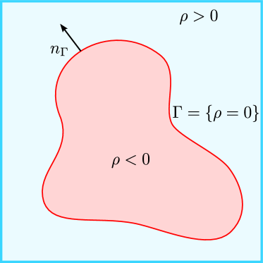
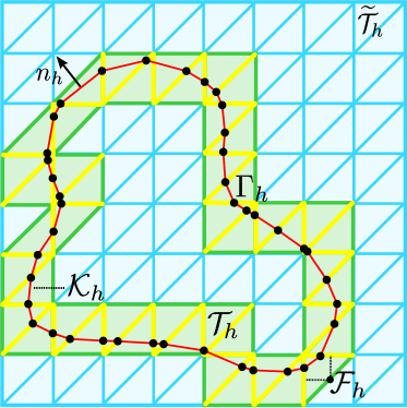
Figure 1: Domain set-up

We observe that the active mesh $\mathcal{T}_{h}$ gives raise to a discrete or approximate $h$-tubular neighborhood of $\Gamma_{h}$, which we denote by

$$\mathcal{T}_{h}=\cup_{T\in\mathcal{T}_{h}}T$$ (2.17)

Note that for all elements $T\in\mathcal{T}_{h}$ there is a neighbor $T^{\prime}\in\mathcal{T}_{h}$ such that $T$ and $T^{\prime}$ share a face. Finally, let

$$V_{h}=\{v\in C(\mathcal{T}_{h}):v|_{T}\in P_{1}(T)\}$$ (2.18)

be the space of continuous piecewise linear polynomials defined on $\mathcal{T}_{h}$ and define the discrete counterpart of $H^{1}(\Gamma)/\mathbb{R}$ by

$$V_{h,0}=\{v\in V_{h}:\lambda_{\Gamma_{h}}(v)=0\}$$ (2.19)

consisting of those $v\in V_{h}$ with zero average $\lambda_{\Gamma_{h}}(v)=\int_{\Gamma_{h}}v$.

2.4 The Full Gradient Stabilized Cut Finite Element Method

As the discrete counterpart of the bilinear form $a(\cdot,\cdot)$ we consider, similar to [25], both a tangential and full gradient variant,

$$a_{h}^{1}(v,w) =(\nabla_{\Gamma_{h}}v,\nabla_{\Gamma_{h}}w)_{\mathcal{K}_{h}}$$ (2.20)

$$a_{h}^{2}(v,w) =(\nabla v,\nabla w)_{\mathcal{K}_{h}}$$ (2.21)

Defining the discrete linear form

$$l_{h}(v)=(f^{e},v)_{\mathcal{K}_{h}}$$ (2.22)

the full gradient stabilized cut finite element method for the Laplace-Beltrami problem (2.7) takes the form: find $u_{h}\in V_{h,0}$ such that for $i=1,2$

$$A_{h}^{i}(u_{h},v)=l_{h}(v)\quad\forall v\in V_{h,0}$$ (2.23)

with

$$A_{h}^{i}(v,w)=a_{h}^{i}(v,w)+\tau s_{h}(v,w)\quad\forall v,w\in V_{h}$$ (2.24)

where $\tau$ is a positive parameter and $s_{h}(\cdot,\cdot)$ is the full gradient stabilization defined by

$$s_{h}(v,w) =h(\nabla v,\nabla w)_{\mathcal{T}_{h}}$$ (2.25)

As the forthcoming a priori error and condition number analysis of the first formulation will be covered by the analysis of the second, we will from now focus on the latter one and omit the superscript $i$. We introduce the stabilization norm

$$\|v\|_{s_{h}}^{2}=s_{h}(v,v)$$ (2.26)

as well as the following energy norms for $v\in H^{1}(\Gamma)+V_{h}^{l}$ and $w\in H^{1}(\Gamma)^{e}+V_{h}$

$$\|v\|_{a}^{2}=a(v,v),\quad\|w\|_{a_{h}}^{2}=a_{h}(w,w),\quad\|w\|_{A_{h}}^{2}=A_{h}(w,w)=\|w\|_{a_{h}}^{2}+\|w\|_{s_{h}}^{2}$$ (2.27)

Clearly, the bilinear form (2.24) is both coercive and continuous with respect to $\|\cdot\|_{A_{h}}$:

$$\|v\|_{A_{h}}^{2} \lesssim A_{h}(v,v)\qquad$$ (2.28)

$$A_{h}(v,w) \lesssim\|v\|_{A_{h}}\|w\|_{A_{h}}$$ (2.29)

3 Preliminaries

3.1 Trace Estimates and Inverse Inequalities

First, we recall the following trace inequality for $v\in H^{1}(\mathcal{T}_{h})$

$$\|v\|_{\partial T}\lesssim h^{-1/2}\|v\|_{T}+h^{1/2}\|\nabla v\|_{T}\quad\forall\,T\in\mathcal{T}_{h}$$ (3.1)

while for the intersection $\Gamma\cap T$ the corresponding inequality

$$\|v\|_{\Gamma\cap T}\lesssim h^{-1/2}\|v\|_{T}+h^{1/2}\|\nabla v\|_{T}\quad\forall\,T\in\mathcal{T}_{h}$$ (3.2)

holds whenever $h$ is small enough, see [15] for a proof. In the following, we will also need some well-known inverse estimates for $v_{h}\in V_{h}$:

$$\|\nabla v_{h}\|_{T}\lesssim h^{-1}\|v_{h}\|_{T}\quad\forall\,T\in\mathcal{T}_{h}$$ (3.3)

$$\|v_{h}\|_{\partial T}\lesssim h^{-1/2}\|v_{h}\|_{T},\qquad\|\nabla v_{h}\|_{\partial T}\lesssim h^{-1/2}\|\nabla v_{h}\|_{T}\quad\forall\,T\in\mathcal{T}_{h}$$ (3.4)

and the following “cut versions” when $K\cap T\not\subseteq\partial T$

$$\|v_{h}\|_{K\cap T} \lesssim h^{-1/2}\|v_{h}\|_{T}, \qquad\|\nabla v_{h}\|_{K\cap T} \lesssim h^{-1/2}\|\nabla v_{h}\|_{T} \quad\forall\,K\in\mathcal{K}_{h},\;\forall\,T\in\mathcal{T}_{h}$$ (3.5)

which are an immediate consequence of similar inverse estimates presented in [15].

3.2 Geometric Estimates

We now recall some standard geometric identities and estimates which typically are used in numerical analysis of the discrete scheme when passing from the discrete surface to the continuous one and vice versa. For a detailed derivation, we refer to Dziuk [9], Olshanskii et al. [21], Dziuk and Elliott [10]. Starting with the Hessian of the signed distance function

$$\mathcal{H}=\nabla\otimes\nabla\rho\quad\text{on }U_{\delta_{0}}(\Gamma)$$ (3.6)

the derivative of the closest point projection and of an extended function $v^{e}$ is given by

$$Dp={P}_{\Gamma}(I-\rho\mathcal{H})={P}_{\Gamma}-\rho\mathcal{H}$$ (3.7)

$$Dv^{e}=D(v\circ p)=DvDp=DvP_{\Gamma}(I-\rho\mathcal{H})$$ (3.8)

The self-adjointness of ${P}_{\Gamma}$, ${P}_{\Gamma_{h}}$, and $\mathcal{H}$, and the fact that ${P}_{\Gamma}\mathcal{H}=\mathcal{H}=\mathcal{H}{P}_{\Gamma}$ and ${P}_{\Gamma}^{2}={P}_{\Gamma}$ then leads to the identities

$$\nabla v^{e} ={P}_{\Gamma}(I-\rho\mathcal{H})\nabla v={P}_{\Gamma}(I-\rho\mathcal{H})\nabla_{\Gamma}v$$ (3.9)

$$\nabla_{\Gamma_{h}}v^{e} ={P}_{\Gamma_{h}}(I-\rho\mathcal{H}){P}_{\Gamma}\nabla v=B^{T}\nabla_{\Gamma}v$$ (3.10)

where the invertible linear mapping

$$B=P_{\Gamma}(I-\rho H)P_{\Gamma_{h}}:T_{x}({\Gamma_{h}})\to T_{p(x)}(\Gamma)$$ (3.11)

maps the tangential space of $\Gamma_{h}$ at $x$ to the tangential space of $\Gamma$ at $p(x)$. Setting $v=w^{l}$ and using the identity $(w^{l})^{e}=w$, we immediately get that

$$\nabla_{\Gamma}w^{l}=B^{-T}\nabla_{\Gamma_{h}}w$$ (3.12)

for any elementwise differentiable function $w$ on $\Gamma_{h}$ lifted to $\Gamma$. We recall from [13, Lemma 14.7] that for $x\in U_{\delta_{0}}(\Gamma)$, the Hessian $\mathcal{H}$ admits a representation

$$\mathcal{H}(x)=\sum_{i=1}^{d}\frac{\kappa_{i}^{e}}{1+\rho(x)\kappa_{i}^{e}}a_{i}^{e}\otimes a_{i}^{e}$$ (3.13)

where $\kappa_{i}$ are the principal curvatures with corresponding principal curvature vectors $a_{i}$. Thus

$$\|\mathcal{H}\|_{L^{\infty}(U_{\delta_{0}}(\Gamma))}\lesssim 1$$ (3.14)

for $\delta_{0}>0$ small enough and as a consequence the following bounds for the linear operator $B$ can be derived (see [9, 10] for the details):

Lemma 3.1

It holds

$$\|B\|_{L^{\infty}(\Gamma_{h})}\lesssim 1,\quad\|B^{-1}\|_{L^{\infty}(\Gamma)}\lesssim 1,\quad\|P_{\Gamma}-BB^{T}\|_{L^{\infty}(\Gamma)}\lesssim h^{2}$$ (3.15)

In the course of the a priori analysis in Section 6, we will need to quantify the error introduced by using the full gradient in (2.21) instead of $\nabla_{\Gamma_{h}}$. To do so we decompose the full gradient as $\nabla=\nabla_{\Gamma_{h}}+{Q}_{\Gamma_{h}}\nabla$ with ${Q}_{\Gamma_{h}}=I-{P}_{\Gamma_{h}}=n_{h}\otimes n_{h}$. We then have

Lemma 3.2

For $v\in H^{1}(\Gamma)$ it holds

$$\|{Q}_{\Gamma_{h}}\nabla v^{e}\|_{\Gamma}\lesssim h\|\nabla_{\Gamma}v\|_{\Gamma}$$ (3.16)

Proof 1

Since $\nabla v^{e}$ = ${P}_{\Gamma}(I-\rho\mathcal{H})\nabla_{\Gamma}v$ according to identity (3.9), it is enough to prove that

$$\|{Q}_{\Gamma_{h}}{P}_{\Gamma}\|_{L^{\infty}(\Gamma)}\lesssim h$$ (3.17)

But a simple computation shows that

$$\|{Q}_{\Gamma_{h}}{P}_{\Gamma}\|_{L^{\infty}(\Gamma)} =\|n_{h}\otimes n_{h}-(n_{h},n)_{\mathbb{R}^{d}}n_{h}\otimes n\|_{L^{\infty}(\Gamma)}$$ (3.18)

$$=\|(1-(n_{h},n)_{\mathbb{R}^{d}})n_{h}\otimes n_{h}\|_{L^{\infty}(\Gamma)}+\|(n_{h},n)_{\mathbb{R}^{d}}n_{h}\otimes(n_{h}-n)\|_{L^{\infty}(\Gamma)}$$ (3.19)

$$\lesssim h^{2}+h$$ (3.20)

Next, for a subset $\omega\subset{\Gamma_{h}}$, we have the change of variables formula

$$\int_{\omega^{l}}g^{l}d\Gamma=\int_{\omega}g|B|d\Gamma_{h}$$ (3.21)

with $|B|$ denoting the absolute value of the determinant of $B$. The determinant $|B|$ satisfies the following estimates.

Lemma 3.3

It holds

$$\|1-|B|\|_{L^{\infty}(\mathcal{K}_{h})} \lesssim h^{2}, \qquad\||B|\|_{L^{\infty}(\mathcal{K}_{h})} \lesssim 1, \qquad\||B|^{-1}\|_{L^{\infty}(\mathcal{K}_{h})} \lesssim 1$$ (3.22)

Combining the various estimates for the norm and the determinant of $B$ shows that for $m=0,1$

$$\|v\|_{H^{m}(\mathcal{K}_{h}^{l})} \sim\|v^{e}\|_{H^{m}(\mathcal{K}_{h})} \quad\text{for }v\in H^{m}(\mathcal{K}_{h}^{l})$$ (3.23)

$$\|w^{l}\|_{H^{m}(\mathcal{K}_{h}^{l})} \sim\|w\|_{H^{m}(\mathcal{K}_{h})} \quad\text{for }w\in V_{h}$$ (3.24)

Next, we observe that thanks to the coarea-formula (cf. Evans and Gariepy [12])

$$\int_{U_{\delta}}f(x)\,dx=\int_{-\delta}^{\delta}\left(\int_{\Gamma(r)}f(y,r)\,\mathrm{d}\Gamma_{r}(y)\right)\,\mathrm{d}r$$

the extension operator $v^{e}$ defines a bounded operator $H^{m}(\Gamma)\ni v\mapsto v^{e}\in H^{m}(U_{\delta}(\Gamma))$ satisfying the stability estimate

$$\|v^{e}\|_{k,U_{\delta}(\Gamma)}\lesssim\delta^{1/2}\|v\|_{k,\Gamma},\qquad 0\leqslant k\leqslant m$$ (3.25)

for $0<\delta\leqslant\delta_{0}$ where the hidden constant depends only on the curvature of $\Gamma$.

3.3 Interpolation Operator

Next, we recall from Scott and Zhang [26] that for $v\in H^{m}(\mathcal{T}_{h})$, the standard Scott-Zhang interpolant $\pi_{h}:L^{2}(\mathcal{T}_{h})\rightarrow V_{h}$ satisfies the local interpolation estimates

$$\|v-\pi_{h}v\|_{k,T} \lesssim h^{l-k}|v|_{l,\omega(T)}, \quad 0\leqslant k\leqslant l\leqslant\min\{2,m\}\quad \forall\,T\in\mathcal{T}_{h}$$ (3.26)

$$\|v-\pi_{h}v\|_{l,F} \lesssim h^{l-k-1/2}|v|_{l,\omega(F)}, \quad 0\leqslant k\leqslant l-1/2\leqslant\min\{2,m\}-1/2\quad \forall\,F\in\mathcal{F}_{h}$$ (3.27)

where $\omega(T)$ consists of all elements sharing a vertex with $T$. The patch $\omega(F)$ is defined analogously. Now with the help of the extension operator, an interpolation operator $\pi_{h}:H^{m}(\Gamma)\to V_{h}$ can be constructed by setting $\pi_{h}v=\pi_{h}v^{e}$, where we took the liberty of using the same symbol. Choosing $\delta_{0}\sim h$, it follows directly from combining the trace inequality (3.2), the interpolation estimate (3.27), and the stability estimate (3.25) that the interpolation operator satisfies the following error estimate:

Lemma 3.4

For $v\in H^{2}(\Gamma)$, it holds that

$$h\|v^{e}-\pi_{h}v^{e}\|_{{\Gamma_{h}}}+\|v^{e}-\pi_{h}v^{e}\|_{a_{h}} \lesssim h\|v\|_{2,\Gamma}$$ (3.28)

3.4 Fat Intersection Covering

Since the surface geometry is represented on fixed background mesh, the active mesh $\mathcal{T}_{h}$ might contain elements which barely intersects the discretized surface $\Gamma_{h}$. Such “small cut elements” typically prohibit the application of a whole set of well-known estimates, such as interpolation estimates and inverse inequalities, which rely on certain scaling properties. As a partial replacement for the lost scaling properties we here recall from Burman et al. [2] the concept of fat intersection coverings of $\mathcal{T}_{h}$.

In Burman et al. [2] it was proved that the active mesh fulfills a fat intersection property which roughly states that for every element in $\mathcal{T}_{h}$ there is a close-by element which has a significant intersection with $\Gamma_{h}$. More precisely, let $x$ be a point on $\Gamma$ and let $B_{\delta}(x)=\{y\in\mathbb{R}^{d}:|x-y|<\delta\}$ and $D_{\delta}=B_{\delta}(x)\cap\Gamma$. We define the sets of elements

$$\mathcal{K}_{\delta,x}=\{K\in\mathcal{K}_{h}:\overline{K}^{l}\cap D_{\delta}(x)\neq\emptyset\},\qquad\mathcal{T}_{\delta,x}=\{T\in\mathcal{T}_{h}:T\cap\Gamma_{h}\in\mathcal{K}_{\delta,x}\}$$ (3.29)

With $\delta\sim h$ we use the notation $\mathcal{K}_{h,x}$ and $\mathcal{T}_{h,x}$. For each $\mathcal{T}_{h}$, $h\in(0,h_{0}]$ there is a set of points $\mathcal{X}_{h}$ on $\Gamma$ such that $\{\mathcal{K}_{h,x},x\in\mathcal{X}_{h}\}$ and $\{\mathcal{T}_{h,x},x\in\mathcal{X}_{h}\}$ are coverings of $\mathcal{T}_{h}$ and $\mathcal{K}_{h}$ with the following properties:

• The number of set containing a given point $y$ is uniformly bounded

  $$\#\{x\in\mathcal{X}_{h}:y\in\mathcal{T}_{h,x}\}\lesssim 1\quad\forall\,y\in\mathbb{R}^{d}$$ (3.30)

  for all $h\in(0,h_{0}]$ with $h_{0}$ small enough.

• The number of elements in the sets $\mathcal{T}_{h,x}$ is uniformly bounded

  $$\#\mathcal{T}_{h,x}\lesssim 1\quad\forall\,x\in\mathcal{X}_{h}$$ (3.31)

  for all $h\in(0,h_{0}]$ with $h_{0}$ small enough, and each element in $\mathcal{T}_{h,x}$ shares at least one face with another element in $\mathcal{T}_{h,x}$.

• $\forall\,h\in(0,h_{0}]$ with $h_{0}$ small enough, and $\forall\,x\in\mathcal{X}_{h}$, $\exists T_{x}\in\mathcal{T}_{h,x}$ that has a large (fat) intersection with $\Gamma_{h}$ in the sense that

  $$|T_{x}|\sim h|T_{x}\cap\Gamma_{h}|=h|K_{x}|\quad\forall\,x\in\mathcal{X}_{h}$$ (3.32)

To make use of the fat intersection property in the next section, we will need the following Lemma 3.5 which describes how the control of discrete functions on potentially small cut elements can be transferred to their close-by neighbors with large intersection by using a face-based stabilization term. A proof of the first estimate can be found in Massing et al. [18].

Lemma 3.5

Let $v\in V_{h}$ and consider a macro-element $\mathcal{M}=T_{1}\cup T_{2}$ formed by any two elements $T_{1}$ and $T_{2}$ of $\mathcal{T}_{h}$ sharing a face $F$. Then

$$\|v\|_{T_{1}}^{2} \lesssim\|v\|_{T_{2}}^{2}+h^{3}\|n_{F}\cdot[\nabla v]\|_{F}^{2}$$ (3.33)

with the hidden constant only depending on the quasi-uniformness parameter.

4 Stability and Condition Number estimates

4.1 Discrete Poincaré Estimates

First we recall that $v\in V_{h}$ satisfies a Poincaré inequality on the surface (see [2, Lemma 4.1]):

Lemma 4.1

For $v\in V_{h}$, the following estimate holds

$$\|v-\lambda_{\Gamma_{h}}(v)\|_{\Gamma_{h}}\lesssim\|\nabla_{\Gamma_{h}}v\|_{\Gamma_{h}}$$ (4.1)

for $0<h\leq h_{0}$ with $h_{0}$ small enough.

Next, we derive an additional Poincaré inequality which involves a scaled version of the $L^{2}$ norm of discrete finite element functions on the active mesh.

Lemma 4.2

For $v\in V_{h}$, the following estimate holds

$$h^{-1}\|v-\lambda_{\Gamma_{h}}(v)\|^{2}_{\mathcal{T}_{h}}\lesssim\|\nabla_{\Gamma_{h}}v\|_{\Gamma_{h}}^{2}+h\|\nabla v\|_{\mathcal{T}_{h}}^{2}$$ (4.2)

for $0<h\leq h_{0}$ with $h_{0}$ small enough.

Proof 2

Without loss of generality we can assume that $\lambda_{\Gamma_{h}}(v)=0$. Apply (3.33) and (3.4) to obtain

$$\|v\|_{\mathcal{T}_{h}}^{2} \lesssim\sum_{x\in\mathcal{X}_{h}}\|v\|_{\mathcal{T}_{h,x}}^{2}\lesssim\sum_{x\in\mathcal{X}_{h}}\|v\|_{T_{x}}^{2}+h^{3}\|n_{F}\cdot[\nabla v]\|_{\mathcal{F}_{h}}^{2}\lesssim\sum_{x\in\mathcal{X}_{h}}\|v\|_{T_{x}}^{2}+h^{2}\|\nabla v\|_{\mathcal{T}_{h}}^{2}$$ (4.3)

Thus it is sufficient to estimate the first term in (4.3). For $v\in V_{h}$, we define a piecewise constant version satisfying $\overline{v}|_{T}=\tfrac{1}{|T|}\int_{T}v\,\mathrm{d}x$. Clearly $\|v-\overline{v}\|_{T}\lesssim h\|\nabla v\|_{T}$. Adding and subtracting $\overline{v}$ gives

$$\sum_{x\in\mathcal{X}_{h}}\|v\|_{T_{x}}^{2} \lesssim\sum_{x\in\mathcal{X}_{h}}\|v-\overline{v}\|_{T_{x}}^{2}+\sum_{x\in\mathcal{X}_{h}}\|\overline{v}\|_{T_{x}}^{2}$$ (4.4)

$$\lesssim h^{2}\|\nabla v\|_{\mathcal{T}_{h}}^{2}+\sum_{x\in\mathcal{X}_{h}}h\|\overline{v}\|_{K_{x}}^{2}$$ (4.5)

$$\lesssim h^{2}\|\nabla v\|_{\mathcal{T}_{h}}^{2}+h\|v\|_{\Gamma_{h}}^{2}+\underbrace{h\|v-\overline{v}\|_{\Gamma_{h}}^{2}}_{\lesssim h^{2}\|\nabla v\|_{\mathcal{T}_{h}}^{2}}$$ (4.6)

$$\lesssim h^{2}\|\nabla v\|_{\mathcal{T}_{h}}^{2}+h\|\nabla_{\Gamma_{h}}v\|_{\Gamma_{h}}^{2}$$ (4.7)

where in the last step, the Poincaré inequality (4.1) was applied.

Remark 5

In Burman et al. [2], the discrete bilinear form $a^{1}(v,w)=(\nabla_{\Gamma_{h}}v,\nabla_{\Gamma_{h}})_{\mathcal{K}_{h}}$ was augmented with the face-based stabilization term

$$\tau j_{h}(v,w)=\tau(n_{F}\cdot[\nabla v],n_{F}\cdot[\nabla w])_{\mathcal{F}_{h}}$$ (5.1)

to prove optimal a priori error and condition number estimates using a discrete Poincaré inequality of the form

$$h^{-1}\|v-\lambda_{\Gamma_{h}}(v)\|^{2}_{\mathcal{T}_{h}}\lesssim\|\nabla_{\Gamma_{h}}v\|_{\Gamma_{h}}^{2}+\|n_{F}\cdot[\nabla v]\|_{\mathcal{F}_{h}}^{2}$$ (5.2)

for $v\in V_{h}$. As before, $\tau$ denotes a positive stabilization parameter which has to be chosen large enough.

Compared to the face-based stabilization (5.1), the full gradient stabilization (2.25) has three main advantages: Firstly, its implementation is extremely cheap and immediately available in many finite element codes. Secondly, the stencil of the discretization operator is not enlarged, as opposed to using a face-based penalty operator. Thirdly, anticipating the numerical results in Section 8, the accuracy and conditioning of a full gradient stabilized surface method is less sensitive to the choice of the stability parameter $\tau$ than for a face-based stabilized scheme.

5.1 Bounds for the Condition Number

With the help of the Poincaré estimates derived in the previous section, we now show that the condition number of the stiffness matrix associated with the bilinear form (2.23) can be bounded by $O(h^{-2})$ independently of the position of the surface $\Gamma$ relative to the background mesh $\mathcal{T}_{h}$. Let $\{\phi_{i}\}_{i=1}^{N}$ be the standard piecewise linear basis functions associated with $\mathcal{T}_{h}$ and thus $v=\sum_{i=1}^{N}V_{i}\phi_{i}$ for $v\in V_{h}$ and expansion coefficients $V=\{V_{i}\}_{i=1}^{N}\in\mathbb{R}^{N}$. The stiffness matrix $\mathcal{A}$ is given by the relation

$$(\mathcal{A}V,W)_{\mathbb{R}^{N}}=A_{h}(v,w)\quad\forall\,v,w\in V_{h}$$ (5.3)

Recalling the definition of $V_{h,0}$ the stiffness matrix $\mathcal{A}$ clearly is a bijective linear mapping $\mathcal{A}:\widehat{\mathbb{R}}^{N}\to\ker(\mathcal{A})^{\perp}$ where we set $\widehat{\mathbb{R}}^{N}=\mathbb{R}^{N}/\ker(\mathcal{A})$ to factor out the one-dimensional kernel given by $\ker{\mathcal{A}}=\operatorname{span}\{(1,\ldots,1)^{\top}\}$. The operator norm and condition number of the matrix $\mathcal{A}$ are then defined by

$$\|\mathcal{A}\|_{\mathbb{R}^{N}}=\sup_{V\in\widehat{\mathbb{R}}^{N}\setminus\boldsymbol{0}}\dfrac{\|\mathcal{A}V\|_{\mathbb{R}^{N}}}{\|V\|_{\mathbb{R}^{N}}}\quad\text{and}\quad\kappa(\mathcal{A})=\|\mathcal{A}\|_{\mathbb{R}^{N}}\|\mathcal{A}^{-1}\|_{\mathbb{R}^{N}}$$ (5.4)

respectively. Following the approach in Ern and Guermond [11], a bound for the condition number can be derived by combining the well-known estimate

$$h^{d/2}\|V\|_{\mathbb{R}^{N}}\lesssim\|v_{h}\|_{L^{2}(\mathcal{T}_{h})}\lesssim h^{d/2}\|V\|_{\mathbb{R}^{N}}$$ (5.5)

which holds for any quasi-uniform mesh $\mathcal{T}_{h}$, with the Poincaré-type estimate (4.2) and the following inverse estimate:

Lemma 5.1

Let $v\in V_{h,0}$ then the following inverse estimate holds

$$\|v\|_{A_{h}}\lesssim h^{-3/2}\|v\|_{\mathcal{T}_{h}}$$ (5.6)

Proof 3

Recall that $\|v\|_{A_{h}}=\|v\|_{a_{h}}+\|v\|_{s_{h}}$. First, employ the standard inverse estimate (3.3) to obtain

$$\|v\|_{s_{h}}^{2}=h\|\nabla v\|_{\mathcal{T}_{h}}^{2}\lesssim h^{-1}\|v\|_{\mathcal{T}_{h}}^{2}$$ (5.7)

Next, the inverse estimates (3.5) and (3.3) gives

$$\|v\|_{a_{h}}^{2}=\|\nabla v\|_{\mathcal{K}_{h}}^{2}\lesssim h^{-1}\|\nabla v\|_{\mathcal{T}_{h}}^{2}\lesssim h^{-3}\|v\|_{\mathcal{T}_{h}}^{2}$$ (5.8)

which concludes the proof.

We are now in the position to prove the main result of this section:

Theorem 5.1

The condition number of the stiffness matrix satisfies the estimate

$$\kappa(\mathcal{A})\lesssim h^{-2}$$ (5.9)

where the hidden constant depends only on the quasi-uniformness parameters.

Proof 4

We need to bound $\|\mathcal{A}\|_{\mathbb{R}^{N}}$ and $\|\mathcal{A}^{-1}\|_{\mathbb{R}^{N}}$. First observe that for $w\in V_{h}$,

$$\|w\|_{A_{h}}\lesssim h^{-3/2}\|w\|_{\mathcal{T}_{h}}\lesssim h^{(d-3)/2}\|W\|_{\mathbb{R}^{N}}$$ (5.10)

where the inverse estimate (5.6) and equivalence (5.5) were successively used. Thus

$$\|\mathcal{A}V\|_{\mathbb{R}^{N}} =\sup_{W\in\mathbb{R}^{N}}\frac{(\mathcal{A}V,W)_{\mathbb{R}^{N}}}{\|W\|_{\mathbb{R}^{d}}}=\sup_{w\in V_{h}}\frac{A_{h}(v,w)}{\|w\|_{A_{h}}}\frac{\|w\|_{A_{h}}}{\|W\|_{\mathbb{R}^{N}}}\lesssim h^{(d-3)/2}\|v\|_{A_{h}}\lesssim h^{d-3}\|V\|_{\mathbb{R}^{N}}$$ (5.11)

and thus by the definition of the operator norm, $\|\mathcal{A}\|_{\mathbb{R}^{N}}\lesssim h^{d-3}$. To estimate $\|\mathcal{A}^{-1}\|_{\mathbb{R}^{N}}$, start from (5.5) and combine the Poincaré inequality (4.2) with a Cauchy-Schwarz inequality to arrive at the following chain of estimates:

$$\|V\|^{2}_{\mathbb{R}^{N}}\lesssim h^{-d}\|v\|^{2}_{\mathcal{T}_{h}}\lesssim h^{1-d}A_{h}(v,v)=h^{1-d}(V,\mathcal{A}V)_{\mathbb{R}^{N}}\lesssim h^{1-d}\|V\|_{\mathbb{R}^{N}}\|\mathcal{A}V\|_{\mathbb{R}^{N}}$$ (5.12)

and hence $\|V\|_{\mathbb{R}^{N}}\lesssim h^{1-d}\|\mathcal{A}V\|_{\mathbb{R}^{N}}$. Now setting $V=\mathcal{A}^{-1}W$ we conclude that $\|\mathcal{A}^{-1}\|_{\mathbb{R}^{N}}\lesssim h^{1-d}$ and combining estimates for $\|\mathcal{A}\|_{\mathbb{R}^{N}}$ and $\|\mathcal{A}^{-1}\|_{\mathbb{R}^{N}}$ the theorem follows.

6 A Priori Error Estimates

This section is devoted to the proof of the main a priori estimates for the weak formulation (2.23). We proceed in two steps. First, we establish an abstract Strang-type lemma which reveals that the overall error can be split into an interpolation error and a consistency error. Next, we provide a bound for the consistency error in order to complete the a priori estimate of the energy norm error. Finally, using a duality argument, we establish an optimal $L^{2}$ error bound where we use the smoothness of the dual function to obtain sufficient control of the consistency error.

6.1 Strang’s Lemma

Lemma 6.1

With $u$ the solution of (2.7) and $u_{h}$ the solution of (2.23) it holds

$$\|u^{e}-u_{h}\|_{A_{h}} \leqslant 2\|u^{e}-\pi_{h}u^{e}\|_{A_{h}}+\sup_{v\in V_{h}}\dfrac{l_{h}(v)-A_{h}(u^{e},v)}{\|v\|_{A_{h}}}$$ (6.1)

Proof 5

Thanks to triangle inequality $\|u^{e}-u_{h}\|_{A_{h}}\leqslant\|u^{e}-\pi_{h}u^{e}\|_{A_{h}}+\|u_{h}-\pi_{h}u^{e}\|_{A_{h}}$, it is sufficient to consider the discrete error $e_{h}=u_{h}-\pi_{h}u^{e}$. Now observe that

$$\|e_{h}\|_{A_{h}}^{2} =A_{h}(u_{h}-\pi_{h}u^{e},e_{h})$$ (6.2)

$$=l_{h}(e_{h})-A_{h}(u^{e},e_{h})+A_{h}(u^{e}-\pi_{h}u^{e},e_{h})$$ (6.3)

$$\lesssim\sup_{v\in V_{h}}\dfrac{l_{h}(v)-A_{h}(u^{e},v)}{\|v\|_{A_{h}}}+\sup_{v\in V_{h}}\dfrac{A_{h}(u^{e}-\pi_{h}u^{e},v)}{\|v\|_{A_{h}}}$$ (6.4)

and apply a Cauchy-Schwarz inequality on the second term in (6.4) to conclude the proof.

6.2 Consistency Error Estimates

Next, we derive a representation of the consistency error, showing that it can be attributed to a geometric error and a consistency error introduced by the stabilization form $s_{h}$.

Lemma 6.2

Let $v\in V_{h}$ and $\phi\in H^{2}(\Gamma)$, then the following estimates hold

$$|l_{h}(v)-A_{h}(u^{e},v)| \lesssim h\|f\|_{\Gamma}\|v\|_{A_{h}}$$ (6.5)

$$|l_{h}(\pi_{h}\phi^{e})-A_{h}(u^{e},\pi_{h}\phi^{e})| \lesssim h^{2}\|f\|_{\Gamma}\|\phi\|_{2,\Gamma}$$ (6.6)

Proof 6

Recalling the definition (2.24) of $A_{h}(\cdot,\cdot)$ and inserting $a(u,v^{l})-l(v^{l})=0$ yields

$$l_{h}(v)-A_{h}(u^{e},v) =\bigl{(}l_{h}(v)-l(v^{l})\bigr{)}+\bigl{(}a(u,v^{l})-a_{h}(u^{e},v)\bigr{)}-s_{h}(u^{e},v)$$ (6.7)

$$=I+II+III$$ (6.8)

which we estimate next.

Term $\boldsymbol{I}$. For the quadrature error of the right hand side we have

$$l(v^{l})-l_{h}(v) =(f,v^{l})_{\Gamma}-(f^{e},v)_{\Gamma_{h}}=(f,v^{l}(1-|B|^{-1}))_{\Gamma}\lesssim h^{2}\|f\|_{\Gamma}\|v^{l}\|_{\Gamma}\lesssim h^{2}\|f\|_{\Gamma}\|v\|_{a_{h}}$$ (6.9)

where in the last step, the Poincaré inequality (4.1) was used after passing from $\Gamma$ to $\Gamma_{h}$.

Term $\boldsymbol{II}$. Using the splitting $\nabla=\nabla_{\Gamma_{h}}+{Q}_{\Gamma_{h}}\nabla$ the discrete form $a_{h}$ can be decomposed as

$$a_{h}(u^{e},v)=(\nabla_{\Gamma_{h}}u^{e},\nabla_{\Gamma_{h}}v)_{\Gamma_{h}}+({Q}_{\Gamma_{h}}\nabla u^{e},{Q}_{\Gamma_{h}}\nabla v)_{\Gamma_{h}}$$ (6.10)

Inserting this identity into $II$ gives

$$II=\bigl{(}(\nabla_{\Gamma}u,\nabla_{\Gamma}v^{l})_{\Gamma}-(\nabla_{\Gamma_{h}}u^{e},\nabla_{\Gamma_{h}}v)_{\Gamma_{h}}\bigr{)}-({Q}_{\Gamma_{h}}\nabla u^{e},{Q}_{\Gamma_{h}}\nabla v)_{\Gamma_{h}}=II_{a}+II_{b}$$ (6.11)

A bound for the first term $II_{a}$ can be derived by lifting the tangential part of $a_{h}(\cdot,\cdot)$ to $\Gamma$ and employing the bound for determinant (3.22) the operator norm estimates (3.15), and the norm equivalences (3.23)–(3.24),

$$II_{a} =(\nabla_{\Gamma}u,\nabla_{\Gamma}v^{l})_{\mathcal{K}_{h}^{l}}-(\nabla_{\Gamma_{h}}u,\nabla_{\Gamma_{h}}v)_{\mathcal{K}_{h}}$$ (6.12)

$$=(\nabla_{\Gamma}u,\nabla_{\Gamma}v^{l})_{\mathcal{K}_{h}^{l}}-((\nabla_{\Gamma_{h}}u)^{l},(\nabla_{\Gamma_{h}}v)^{l}|B|^{-1})_{\mathcal{K}_{h}^{l}}$$ (6.13)

$$=(({P}_{\Gamma}-|B|^{-1}BB^{T})\nabla_{\Gamma}u,\nabla_{\Gamma}v^{l})_{\mathcal{K}_{h}^{l}}$$ (6.14)

$$=(({P}_{\Gamma}-BB^{T})+(1-|B|^{-1})BB^{T})\nabla_{\Gamma}u,\nabla_{\Gamma}v^{l})_{\mathcal{K}_{h}^{l}}$$ (6.15)

$$\lesssim h^{2}\|f\|_{\Gamma}\|\nabla_{\Gamma}v^{l}\|_{\mathcal{K}_{h}^{l}}$$ (6.16)

Turning to the second term $II_{b}$ and applying the inequality (3.16) to ${Q}_{\Gamma_{h}}\nabla u^{e}$ gives

$$II_{b} \lesssim\|{Q}_{\Gamma_{h}}\nabla u^{e}\|_{{\Gamma_{h}}}\|{Q}_{\Gamma_{h}}\nabla v\|_{{\Gamma_{h}}}$$ (6.17)

$$\lesssim h\|f\|_{\Gamma}\|{Q}_{\Gamma_{h}}\nabla v\|_{{\Gamma_{h}}}$$ (6.18)

For general $v\in V_{h}$, the last factor in $II_{b}$ is simply bounded by $\|\nabla v\|_{\Gamma_{h}}$ while in the special case $v=\pi_{h}\phi^{e}$, the interpolation estimate (3.28) and a second application of (3.16) to ${Q}_{\Gamma_{h}}\nabla\phi^{e}$ yields

$$\|{Q}_{\Gamma_{h}}\nabla\pi_{h}\phi^{e}\|_{{\Gamma_{h}}}\lesssim\|{Q}_{\Gamma_{h}}\nabla\phi^{e}\|_{{\Gamma_{h}}}+\|{Q}_{\Gamma_{h}}\nabla(\phi^{e}-\pi_{h}\phi^{e})\|_{{\Gamma_{h}}}\lesssim h\|\phi\|_{2,\Gamma}$$ (6.19)

Term $\boldsymbol{III}$. Combine Cauchy-Schwarz’s inequality with the stability estimate (3.25), choosing $\delta\sim h$, to obtain

$$s_{h}(u^{e},v) =h(\nabla u^{e},\nabla v)_{\mathcal{T}_{h}}\lesssim h^{1/2}\|\nabla u^{e}\|_{\mathcal{T}_{h}}\|v\|_{s_{h}}\lesssim h\|\nabla_{\Gamma}u\|_{\Gamma}\|v\|_{s_{h}}\lesssim h\|f\|_{\Gamma}\|v\|_{s_{h}}$$ (6.20)

Now again considering the case $v=\pi_{h}\phi^{e}$, we can estimate (6.20) further via

$$\|\pi_{h}\phi^{e}\|_{s_{h}}\lesssim h^{1/2}\|\nabla\phi^{e}\|_{U_{\delta}(\Gamma)}+\|\pi_{h}\phi^{e}-\phi^{e}\|_{s_{h}}\lesssim h\|\nabla\phi\|_{\Gamma}+h^{2}\|\phi\|_{2,\Gamma}$$ (6.21)

where we pick a $\delta$ in the stability estimate (3.25) such that $\mathcal{T}_{h}\subseteq U_{\delta}(\Gamma)$ and $\delta\lesssim h$. This concludes the proof.

Remark 7

The previous Lemma shows that the consistency error can be improved by one order of $h$ when the “consistency error functional” $R_{h}(\cdot)=l_{h}(\cdot)-A_{h}(u^{e},\cdot)$ is evaluated for special functions $v\in V_{h}$ which are interpolation of smooth functions $v\in H^{2}(\Gamma)$. It is precisely this improved estimate which will allow us to prove optimal $L^{2}$ error estimates using a duality argument, despite the fact that the consistency error is generally of order $h$.

7.1 A Priori Error Estimates

Theorem 7.1

The following a priori error estimates hold

$$\|u^{e}-u_{h}\|_{A_{h}} \lesssim h\|f\|_{\Gamma}$$ (7.1)

$$\|u^{e}-u_{h}\|_{{\Gamma_{h}}} \lesssim h^{2}\|f\|_{\Gamma}$$ (7.2)

Proof 7

With the elliptic regularity estimate (2.11), (7.1) is a direct consequence of the interpolation estimate and the estimate (6.5) of the consistency error arising in the Strang Lemma 6.1. To prove (7.2), we use the standard Aubin-Nitsche trick in combination with the improved estimate (6.6). More precisly, let $\psi\in L^{2}(\Gamma)$ and take $\phi\in H^{2}(\Gamma)$ satisfying $-\Delta_{\Gamma}\phi=\psi$ and the elliptic regularity estimate $\|\phi\|_{2,\Gamma}\lesssim\|\psi\|_{\Gamma}$. We define $e=u-u_{h}^{l}$ and add and subtract suitable terms to derive the following error representation

$$(e,\psi)_{\Gamma} =a(e,\phi)=a(e,\phi)-A_{h}(e^{e},\phi^{e})+A_{h}(e^{e},\phi^{e})$$ (7.3)

$$=\bigl{(}a(e,\phi)-A_{h}(e^{e},\phi^{e})\bigr{)}+A_{h}(e^{e},\phi^{e}-\pi_{h}\phi^{e})+\bigl{(}A_{h}(u,\pi_{h}\phi^{e})-l_{h}(\pi_{h}\phi^{e})\bigr{)}$$ (7.4)

$$=I+II+III$$ (7.5)

Term $III$ is precisely the one appearing in the improved consistency error estimate (6.6), and consequently

$$III\lesssim h^{2}\|f\|_{\Gamma}\|\phi\|_{2,\Gamma}\lesssim h^{2}\|f\|_{\Gamma}\|\psi\|_{\Gamma}$$ (7.6)

The second term can be estimated by combining interpolation and energy norm estimates:

$$II\lesssim\|u^{e}-u_{h}\|_{A_{h}}\|\phi^{e}-\pi_{h}\phi^{e}\|_{A_{h}}\ \lesssim h\|f\|_{\Gamma}h\|\phi\|_{2,\Gamma}\lesssim h\|f\|_{\Gamma}h\|\psi\|_{\Gamma}$$ (7.7)

To derive a bound for the remaining term $I$, we first split of the error contributions introduced by the normal part of the gradient and the stabilization $s_{h}(\cdot,\cdot)$:

$$I =\bigl{(}(\nabla_{\Gamma}e,\nabla_{\Gamma}\phi)_{\Gamma}-(\nabla_{\Gamma_{h}}e^{e},\nabla_{\Gamma_{h}}\phi^{e})_{\Gamma}\bigr{)}-({Q}_{\Gamma_{h}}\nabla_{\Gamma}e^{e},{Q}_{\Gamma_{h}}\nabla_{\Gamma}\phi^{e})_{\Gamma}-s_{h}(e^{e},\phi^{e})$$ (7.8)

$$=I_{a}+I_{b}+I_{c}$$ (7.9)

Now we proceed exactly as in the proof of Lemma 6.2. More precisely, following the derivation of estimates for Term $II_{a}$ and $II_{b}$ in (6.11), we see that

$$I_{a} \lesssim h^{2}\|\nabla_{\Gamma}e\|_{\Gamma}\|\nabla_{\Gamma}\phi\|_{\Gamma}\lesssim h^{3}\|f\|_{\Gamma}\|\psi\|_{\Gamma}$$ (7.10)

$$I_{b} \lesssim\|\nabla_{\Gamma}e^{e}\|_{{\Gamma_{h}}}\|{Q}_{\Gamma_{h}}\nabla\phi^{e}\|_{{\Gamma_{h}}}\lesssim h\|f\|_{\Gamma}h\|\nabla_{\Gamma}\phi\|_{\Gamma}\lesssim h^{2}\|f\|_{\Gamma}\|\psi\|_{\Gamma}$$ (7.11)

Similar as before, we have

$$I_{c}\lesssim\|e^{e}\|_{s_{h}}h^{1/2}\|\nabla\phi^{e}\|_{\mathcal{T}_{h}}\lesssim h\|f\|_{\Gamma}h\|\nabla\phi\|_{\Gamma}\lesssim h^{2}\|f\|_{\Gamma}\|\psi\|_{\Gamma}$$ (7.12)

Now collecting all the estimates for $I$–$III$, dividing by $\|\psi\|_{\Gamma}$ and taking the supremum over $\psi\in L^{2}(\Gamma)$ concludes the proof.

8 Numerical Results

This section is devoted to a series of numerical experiments which corroborate the theoretical findings and assess the effect of the proposed stabilization on the accuracy of the discrete solution and the conditioning of the discrete system. First, a convergence study for two test cases is conducted, where we also examine and compare the effect of the stabilization parameter on the accuracy of the computed solution. In the second series of experiments, we investigate the sensitivity of the condition number with respect to both the surface positioning in the background mesh and the stabilization parameter $\tau$. In all studies, we compare the proposed full gradient stabilization with alternative approaches to cure the discrete system from being ill-conditioned.

8.1 Convergence Rate Tests

Following the numerical examples presented in [3], we consider two test cases for the Laplace-Beltrami-type problem

$$-\Delta_{\Gamma}u+u=f\quad\text{on }\Gamma$$ (8.1)

with given analytical reference solution $u$ and surface $\Gamma=\{x\in\mathbb{R}^{3}:\phi(x)=0\}$ defined by a known smooth scalar function $\phi$ with $\nabla\phi(x)\neq 0\,\forall x\in\Gamma$. The corresponding right-hand side $f$ can be computed using the following representation of the Laplace-Beltrami operator

$$\Delta_{\Gamma}u=\Delta u-n_{\Gamma}\cdot\nabla\otimes\nabla u\,n_{\Gamma}-\textrm{tr}(\nabla n_{\Gamma})\nabla u\cdot n_{\Gamma}$$ (8.2)

For the first test example (Example 1) we chose

$$\left\{\begin{aligned} u_{1}&=\sin\left(\dfrac{\pi x}{2}\right)\sin\left(\dfrac{\pi y}{2}\right)\sin\left(\dfrac{\pi z}{2}\right)\\ \phi_{1}&=x^{2}+y^{2}+z^{2}-1\end{aligned}\right.$$ (8.3)

while in the second example (Example 2), we consider the problem defined by

$$\left\{\begin{aligned} u_{2}&=xy-5y+z+xz\\ \phi_{2}&=(x^{2}-1)^{2}+(y^{2}-1)^{2}+(z^{2}-1)^{2}+(x^{2}+y^{2}-4)^{2}+(x^{2}+z^{2}-4)^{2}\\ &\quad+(y^{2}+z^{2}-4)^{2}-16\end{aligned}\right.$$ (8.4)

The computed solutions for Example 1 and Example 2 are shown in Figure 2. In the first convergence experiment, the tangential gradient form $a^{1}_{h}(v,w)=(\nabla_{\Gamma_{h}}v,\nabla_{\Gamma}w)_{\mathcal{K}_{h}}$ combined with either the full gradient stabilization $s_{h}$ or the face-based stabilization $j_{h}$ is used. For the second convergence experiment, we consider the full gradient form $a_{h}^{2}(v,w)=(\nabla v,\nabla w)_{\mathcal{K}_{h}}$ instead.

Starting from a structured mesh $\widetilde{\mathcal{T}}_{0}$ for $\Omega=[-a,a]^{3}$ with $a$ large enough such that $\Gamma\subseteq\Omega$, a sequence of meshes $\{\mathcal{T}_{k}\}_{k=0}^{5}$ is generated for each test case by successively refining $\widetilde{\mathcal{T}}_{0}$ and extracting the corresponding active mesh as defined by (2.14). Based on the manufactured exact solutions, the experimental order of convergence (EOC) is then calculated by

$$\text{EOC}(k)=\dfrac{\log(E_{k-1}/E_{k})}{\log(2)}$$

where $E_{k}$ denotes the error of the numerical solution $u_{k}$ at refinement level $k$ measured in either the $\|\cdot\|_{H^{1}(\Gamma_{h})}$ or $\|\cdot\|_{L^{2}(\Gamma_{h})}$ norm. To examine the geometric error contributed to the non-vanishing normal gradient component in the full gradient form $a^{2}_{h}$, we also compute in both convergence studies the error for the unstabilized discretization schemes given by $a^{1}_{h}$ and $a^{2}_{h}$ and $\tau=0$.

For the two test cases, the computed errors for the sequence of refined meshes are summarized in Table 1–2 and Table 3–4, respectively. In all cases, the observed EOC confirms the first-order and second-order convergences rates as predicted by Theorem 7.1 and the corresponding a priori error estimates for the unstabilized full gradient form derived in  [7, 25] and for the face-based stabilized tangential form analyzed in  [2].

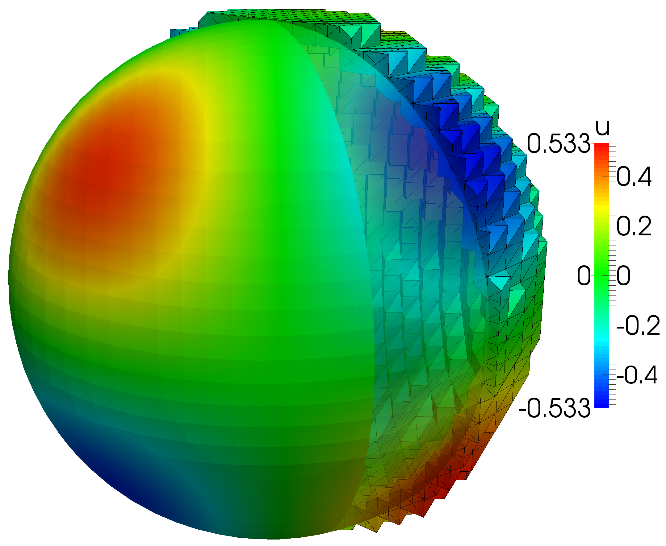
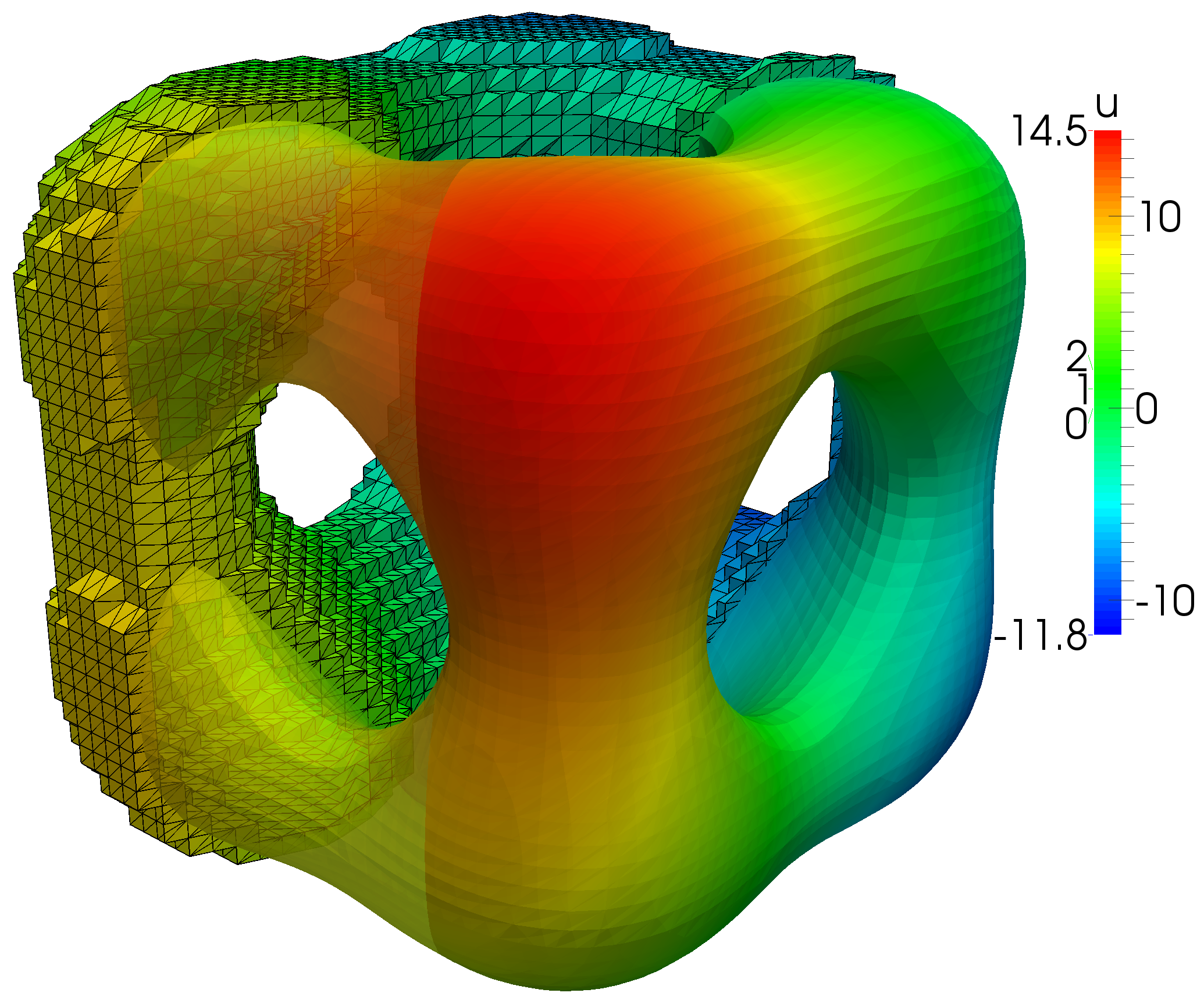
Figure 2: Solution plots from the two convergence studies. Each plot shows both the approximation $u_{h}$ as computed on the active mesh $\mathcal{T}_{h}$ and the restriction of $u_{h}$ to the surface mesh $\mathcal{K}_{h}$. (Left) Solution for Example 1 computed on $\mathcal{T}_{3}$ with $h\approx 7.7\cdot 10^{-2}$ using the face-based stabilized tangential form $a^{1}+\tau j_{h}$ with $\tau=0.01$. (Right) Solution for Example 2 computed on $\mathcal{T}_{3}$ with $h\approx 1.15\cdot 10^{-1}$ using the full gradient stabilized full gradient form $a^{2}+\tau s_{h}$ with $\tau=1.0$.

A closer look at Table 1 reveals that the method based on the unstabilized full gradient form leads, as expected, to a slightly higher error when compared to its tangential gradient counterpart, in agreement with the numerical results presented in [25]. A similar increase of the discretization error can be observed for the second test example, see Table 3.

Turning to the comparison of the full gradient stabilization $s_{h}$ and the face-based stabilization $j_{h}$ presented in Table 2 and Table 4, we observe that the choice of the stabilization parameter $\tau$ is much less critical for the accuracy of full gradient stabilized methods then for the face-based stabilized counterparts, in particular when the error is measured in the $L^{2}$ norm. Indeed, while the $L^{2}$ error increases only by a factor of $\sim$$0.1$ when $\tau$ changes from $0.01$ to $1.0$ in the full gradient stabilization, the error grows by a factor of $\sim$$12$-$14$ when the face-based stabilization is used.

$k$	$\|u_{k}-u\|_{1,\Gamma_{h}}$		EOC	$\|u_{k}-u\|_{\Gamma_{h}}$		EOC
$0$	$1.36$	$\cdot 10^{0}$	–	$2.59$	$\cdot 10^{-1}$	–
$1$	$7.72$	$\cdot 10^{-1}$	$0.82$	$7.39$	$\cdot 10^{-2}$	$1.81$
$2$	$3.85$	$\cdot 10^{-1}$	$1.00$	$1.87$	$\cdot 10^{-2}$	$1.98$
$3$	$1.92$	$\cdot 10^{-1}$	$1.00$	$4.56$	$\cdot 10^{-3}$	$2.04$
$4$	$9.59$	$\cdot 10^{-2}$	$1.00$	$1.13$	$\cdot 10^{-3}$	$2.01$
$5$	$4.80$	$\cdot 10^{-2}$	$1.00$	$2.83$	$\cdot 10^{-4}$	$2.00$

(a) Tangential gradient

$k$	$\|u_{k}-u\|_{1,\Gamma_{h}}$		EOC	$\|u_{k}-u\|_{\Gamma_{h}}$		EOC
$0$	$1.36$	$\cdot 10^{0}$	–	$2.66$	$\cdot 10^{-1}$	–
$1$	$8.70$	$\cdot 10^{-1}$	$0.65$	$1.18$	$\cdot 10^{-1}$	$1.18$
$2$	$4.55$	$\cdot 10^{-1}$	$0.94$	$3.39$	$\cdot 10^{-2}$	$1.79$
$3$	$2.36$	$\cdot 10^{-1}$	$0.95$	$8.99$	$\cdot 10^{-3}$	$1.91$
$4$	$1.19$	$\cdot 10^{-1}$	$0.99$	$2.27$	$\cdot 10^{-3}$	$1.99$
$5$	$5.93$	$\cdot 10^{-2}$	$1.00$	$5.68$	$\cdot 10^{-4}$	$2.00$

(b) Full gradient

Table 1: Convergence rates for Example 1 comparing the unstabilized tangential gradient formulation with the unstabilized full gradient method.

$k$	$\|u_{k}-u\|_{1,\Gamma_{h}}$		EOC	$\|u_{k}-u\|_{\Gamma_{h}}$		EOC
$0$	$1.36$	$\cdot 10^{0}$	–	$2.61$	$\cdot 10^{-1}$	–
$1$	$7.69$	$\cdot 10^{-1}$	$0.82$	$7.54$	$\cdot 10^{-2}$	$1.79$
$2$	$3.84$	$\cdot 10^{-1}$	$1.00$	$1.89$	$\cdot 10^{-2}$	$2.00$
$3$	$1.92$	$\cdot 10^{-1}$	$1.00$	$4.58$	$\cdot 10^{-3}$	$2.04$
$4$	$9.59$	$\cdot 10^{-2}$	$1.00$	$1.13$	$\cdot 10^{-3}$	$2.02$
$5$	$4.80$	$\cdot 10^{-2}$	$1.00$	$2.84$	$\cdot 10^{-4}$	$2.00$

$k$	$\|u_{k}-u\|_{1,\Gamma_{h}}$		EOC	$\|u_{k}-u\|_{\Gamma_{h}}$		EOC
$0$	$1.37$	$\cdot 10^{0}$	–	$2.76$	$\cdot 10^{-1}$	–
$1$	$7.72$	$\cdot 10^{-1}$	$0.83$	$8.58$	$\cdot 10^{-2}$	$1.69$
$2$	$3.83$	$\cdot 10^{-1}$	$1.01$	$2.01$	$\cdot 10^{-2}$	$2.09$
$3$	$1.91$	$\cdot 10^{-1}$	$1.00$	$4.77$	$\cdot 10^{-3}$	$2.07$
$4$	$9.56$	$\cdot 10^{-2}$	$1.00$	$1.16$	$\cdot 10^{-3}$	$2.04$
$5$	$4.79$	$\cdot 10^{-2}$	$1.00$	$2.87$	$\cdot 10^{-4}$	$2.01$

$k$	$\|u_{k}-u\|_{1,\Gamma_{h}}$		EOC	$\|u_{k}-u\|_{\Gamma_{h}}$		EOC
$0$	$1.60$	$\cdot 10^{0}$	–	$3.76$	$\cdot 10^{-1}$	–
$1$	$8.54$	$\cdot 10^{-1}$	$0.90$	$1.44$	$\cdot 10^{-1}$	$1.38$
$2$	$3.95$	$\cdot 10^{-1}$	$1.11$	$2.93$	$\cdot 10^{-2}$	$2.30$
$3$	$1.94$	$\cdot 10^{-1}$	$1.02$	$6.22$	$\cdot 10^{-3}$	$2.24$
$4$	$9.58$	$\cdot 10^{-2}$	$1.02$	$1.36$	$\cdot 10^{-3}$	$2.19$
$5$	$4.77$	$\cdot 10^{-2}$	$1.01$	$3.15$	$\cdot 10^{-4}$	$2.11$

(a) With full gradient stabilization $s_{h}$

$k$	$\|u_{k}-u\|_{1,\Gamma_{h}}$		EOC	$\|u_{k}-u\|_{\Gamma_{h}}$		EOC
$0$	$1.37$	$\cdot 10^{0}$	–	$2.70$	$\cdot 10^{-1}$	–
$1$	$7.71$	$\cdot 10^{-1}$	$0.83$	$8.33$	$\cdot 10^{-2}$	$1.70$
$2$	$3.85$	$\cdot 10^{-1}$	$1.00$	$2.16$	$\cdot 10^{-2}$	$1.95$
$3$	$1.92$	$\cdot 10^{-1}$	$1.00$	$5.36$	$\cdot 10^{-3}$	$2.01$
$4$	$9.58$	$\cdot 10^{-2}$	$1.00$	$1.33$	$\cdot 10^{-3}$	$2.01$
$5$	$4.80$	$\cdot 10^{-2}$	$1.00$	$3.35$	$\cdot 10^{-4}$	$1.99$

$k$	$\|u_{k}-u\|_{1,\Gamma_{h}}$		EOC	$\|u_{k}-u\|_{\Gamma_{h}}$		EOC
$0$	$1.51$	$\cdot 10^{0}$	–	$3.46$	$\cdot 10^{-1}$	–
$1$	$8.46$	$\cdot 10^{-1}$	$0.84$	$1.49$	$\cdot 10^{-1}$	$1.22$
$2$	$4.08$	$\cdot 10^{-1}$	$1.05$	$4.37$	$\cdot 10^{-2}$	$1.76$
$3$	$2.01$	$\cdot 10^{-1}$	$1.02$	$1.15$	$\cdot 10^{-2}$	$1.93$
$4$	$9.96$	$\cdot 10^{-2}$	$1.01$	$2.91$	$\cdot 10^{-3}$	$1.98$
$5$	$4.98$	$\cdot 10^{-2}$	$1.00$	$7.32$	$\cdot 10^{-4}$	$1.99$

$k$	$\|u_{k}-u\|_{1,\Gamma_{h}}$		EOC	$\|u_{k}-u\|_{\Gamma_{h}}$		EOC
$0$	$2.14$	$\cdot 10^{0}$	–	$5.35$	$\cdot 10^{-1}$	–
$1$	$1.71$	$\cdot 10^{0}$	$0.32$	$4.55$	$\cdot 10^{-1}$	$0.24$
$2$	$8.14$	$\cdot 10^{-1}$	$1.07$	$2.07$	$\cdot 10^{-1}$	$1.13$
$3$	$3.07$	$\cdot 10^{-1}$	$1.40$	$6.59$	$\cdot 10^{-2}$	$1.65$
$4$	$1.20$	$\cdot 10^{-1}$	$1.35$	$1.78$	$\cdot 10^{-2}$	$1.88$
$5$	$5.39$	$\cdot 10^{-2}$	$1.16$	$4.56$	$\cdot 10^{-3}$	$1.97$

(b) With face-based stabilization $j_{h}$

Table 2: Convergence rates for Example 1. The solution is computed from a combination of the tangential gradient form $a_{h}^{1}(v,w)=(\nabla_{\Gamma_{h}}v,\nabla_{\Gamma_{h}}w)_{\mathcal{K}_{h}}$ with different stabilizations and penalty parameters. Penalty parameter $\tau$ was set to $\tau=0.01$ (top), $\tau=0.1$ (middle), and $\tau=1.0$ (bottom).

$k$	$\|u_{k}-u\|_{1,\Gamma_{h}}$		EOC	$\|u_{k}-u\|_{\Gamma_{h}}$		EOC
$0$	$2.24$	$\cdot 10^{1}$	–	$1.49$	$\cdot 10^{1}$	–
$1$	$7.92$	$\cdot 10^{0}$	$1.50$	$1.86$	$\cdot 10^{0}$	$3.00$
$2$	$3.48$	$\cdot 10^{0}$	$1.19$	$5.48$	$\cdot 10^{-1}$	$1.76$
$3$	$1.72$	$\cdot 10^{0}$	$1.02$	$1.18$	$\cdot 10^{-1}$	$2.21$
$4$	$8.50$	$\cdot 10^{-1}$	$1.01$	$2.92$	$\cdot 10^{-2}$	$2.02$
$5$	$4.24$	$\cdot 10^{-1}$	$1.00$	$7.32$	$\cdot 10^{-3}$	$1.99$

(a) Tangential gradient

$k$	$\|u_{k}-u\|_{1,\Gamma_{h}}$		EOC	$\|u_{k}-u\|_{\Gamma_{h}}$		EOC
$0$	$2.48$	$\cdot 10^{1}$	–	$1.62$	$\cdot 10^{1}$	–
$1$	$9.30$	$\cdot 10^{0}$	$1.41$	$2.28$	$\cdot 10^{0}$	$2.83$
$2$	$5.48$	$\cdot 10^{0}$	$0.76$	$5.41$	$\cdot 10^{-1}$	$2.07$
$3$	$2.84$	$\cdot 10^{0}$	$0.95$	$1.49$	$\cdot 10^{-1}$	$1.86$
$4$	$1.46$	$\cdot 10^{0}$	$0.96$	$4.06$	$\cdot 10^{-2}$	$1.88$
$5$	$7.38$	$\cdot 10^{-1}$	$0.98$	$1.04$	$\cdot 10^{-2}$	$1.96$

(b) Full gradient

Table 3: Convergence rates for Example 2 comparing the unstabilized tangential gradient formulation with the unstabilized full gradient method.

$k$	$\|u_{k}-u\|_{1,\Gamma_{h}}$		EOC	$\|u_{k}-u\|_{\Gamma_{h}}$		EOC
$0$	$2.49$	$\cdot 10^{1}$	–	$1.63$	$\cdot 10^{1}$	–
$1$	$9.29$	$\cdot 10^{0}$	$1.42$	$2.31$	$\cdot 10^{0}$	$2.82$
$2$	$5.48$	$\cdot 10^{0}$	$0.76$	$5.46$	$\cdot 10^{-1}$	$2.08$
$3$	$2.84$	$\cdot 10^{0}$	$0.95$	$1.50$	$\cdot 10^{-1}$	$1.86$
$4$	$1.46$	$\cdot 10^{0}$	$0.96$	$4.10$	$\cdot 10^{-2}$	$1.88$
$5$	$7.38$	$\cdot 10^{-1}$	$0.98$	$1.05$	$\cdot 10^{-2}$	$1.96$

$k$	$\|u_{k}-u\|_{1,\Gamma_{h}}$		EOC	$\|u_{k}-u\|_{\Gamma_{h}}$		EOC
$0$	$2.61$	$\cdot 10^{1}$	–	$1.76$	$\cdot 10^{1}$	–
$1$	$9.28$	$\cdot 10^{0}$	$1.49$	$2.70$	$\cdot 10^{0}$	$2.71$
$2$	$5.48$	$\cdot 10^{0}$	$0.76$	$6.18$	$\cdot 10^{-1}$	$2.13$
$3$	$2.84$	$\cdot 10^{0}$	$0.95$	$1.69$	$\cdot 10^{-1}$	$1.87$
$4$	$1.46$	$\cdot 10^{0}$	$0.96$	$4.59$	$\cdot 10^{-2}$	$1.89$
$5$	$7.38$	$\cdot 10^{-1}$	$0.98$	$1.17$	$\cdot 10^{-2}$	$1.97$

$k$	$\|u_{k}-u\|_{1,\Gamma_{h}}$		EOC	$\|u_{k}-u\|_{\Gamma_{h}}$		EOC
$0$	$3.55$	$\cdot 10^{1}$	–	$2.66$	$\cdot 10^{1}$	–
$1$	$1.34$	$\cdot 10^{1}$	$1.41$	$8.44$	$\cdot 10^{0}$	$1.66$
$2$	$5.99$	$\cdot 10^{0}$	$1.16$	$2.09$	$\cdot 10^{0}$	$2.01$
$3$	$2.93$	$\cdot 10^{0}$	$1.03$	$5.54$	$\cdot 10^{-1}$	$1.92$
$4$	$1.47$	$\cdot 10^{0}$	$0.99$	$1.43$	$\cdot 10^{-1}$	$1.96$
$5$	$7.39$	$\cdot 10^{-1}$	$0.99$	$3.60$	$\cdot 10^{-2}$	$1.99$

(a) With full gradient stabilization

$k$	$\|u_{k}-u\|_{1,\Gamma_{h}}$		EOC	$\|u_{k}-u\|_{\Gamma_{h}}$		EOC
$0$	$2.47$	$\cdot 10^{1}$	–	$1.63$	$\cdot 10^{1}$	–
$1$	$9.10$	$\cdot 10^{0}$	$1.44$	$2.35$	$\cdot 10^{0}$	$2.79$
$2$	$5.41$	$\cdot 10^{0}$	$0.75$	$5.71$	$\cdot 10^{-1}$	$2.04$
$3$	$2.82$	$\cdot 10^{0}$	$0.94$	$1.63$	$\cdot 10^{-1}$	$1.81$
$4$	$1.45$	$\cdot 10^{0}$	$0.96$	$4.51$	$\cdot 10^{-2}$	$1.86$
$5$	$7.34$	$\cdot 10^{-1}$	$0.98$	$1.16$	$\cdot 10^{-2}$	$1.95$

$k$	$\|u_{k}-u\|_{1,\Gamma_{h}}$		EOC	$\|u_{k}-u\|_{\Gamma_{h}}$		EOC
$0$	$2.43$	$\cdot 10^{1}$	–	$1.68$	$\cdot 10^{1}$	–
$1$	$8.58$	$\cdot 10^{0}$	$1.50$	$2.94$	$\cdot 10^{0}$	$2.52$
$2$	$5.16$	$\cdot 10^{0}$	$0.73$	$8.75$	$\cdot 10^{-1}$	$1.75$
$3$	$2.75$	$\cdot 10^{0}$	$0.91$	$2.97$	$\cdot 10^{-1}$	$1.56$
$4$	$1.42$	$\cdot 10^{0}$	$0.95$	$8.82$	$\cdot 10^{-2}$	$1.75$
$5$	$7.23$	$\cdot 10^{-1}$	$0.98$	$2.36$	$\cdot 10^{-2}$	$1.90$

$k$	$\|u_{k}-u\|_{1,\Gamma_{h}}$		EOC	$\|u_{k}-u\|_{\Gamma_{h}}$		EOC
$0$	$2.49$	$\cdot 10^{1}$	–	$1.88$	$\cdot 10^{1}$	–
$1$	$9.61$	$\cdot 10^{0}$	$1.37$	$5.35$	$\cdot 10^{0}$	$1.81$
$2$	$6.38$	$\cdot 10^{0}$	$0.59$	$2.86$	$\cdot 10^{0}$	$0.90$
$3$	$3.64$	$\cdot 10^{0}$	$0.81$	$1.29$	$\cdot 10^{0}$	$1.15$
$4$	$1.76$	$\cdot 10^{0}$	$1.04$	$4.52$	$\cdot 10^{-1}$	$1.51$
$5$	$8.13$	$\cdot 10^{-1}$	$1.12$	$1.37$	$\cdot 10^{-1}$	$1.73$

(b) With face-based stabilization

Table 4: Convergence rates for Example 2. Solution is computed from a combination of the full gradient form $a_{h}^{2}(v,w)=(\nabla_{\Gamma}v,\nabla_{\Gamma}w)_{\mathcal{K}_{h}}$ with different stabilizations and penalty parameters. Penalty parameter $\tau$ was set to $\tau=0.01$ (top), $\tau=0.1$ (middle), and $\tau=1.0$ (bottom).

8.2 Condition Number Tests

In our final numerical study, the dependency of the condition number on the mesh size and on the positioning of the surface in the background mesh is examined. Additionally, we compare the proposed full gradient stabilization to both face-based stabilized schemes and diagonal preconditioning as alternative approaches to obtain robust and moderate condition numbers for the discrete systems.

We start our numerical experiment by defining a sequence $\{\mathcal{T}_{k}\}_{k=1}^{6}$ of tessellations of $\Omega=[-1.6,1.6]^{3}$ with mesh size $h=3.2/5\cdot 2^{-k/2}$. For each $k$, we generate a family of surfaces $\{\Gamma_{\delta}\}_{0\leqslant\delta\leqslant 1}$ by translating the unit-sphere $S^{2}=\{x\in\mathbb{R}^{3}:\|x\|=1\}$ along the diagonal $(h,h,h)$; that is, $\Gamma_{\delta}=S^{2}+\delta(h,h,h)$ with $\delta\in[0,1]$. For $\delta=l/500$, $l=0,\ldots,500$, we compute the condition number $\kappa_{\delta}(\mathcal{A})$ as the ratio of the absolute value of the largest (in modulus) and smallest (in modulus), non-zero eigenvalue. For the full gradient stabilized full gradient method with $\tau=1.0$, the minimum, maximum, and the arithmetic mean of the resulting scaled condition numbers $h^{2}\kappa_{\delta}(A)$ for each mesh size $h$ are shown in Table 5.

The computed figures in Table 5 clearly confirm the theoretically proven $O(h^{-2})$ bound, independent of the location of the surface in the background mesh. Additionally, Figure 3 confirms for $\mathcal{T}_{2}$ the robustness of the condition number with respect to the translation parameter $\delta$. In contrast, the condition number is highly sensitive and clearly unbounded as a function of $\delta$ if we set the penalty parameter $\tau$ in (2.24) to $0$ as the corresponding plot in Figure 3 shows. The same figure also demonstrates that the discrete system can be made robust by either diagonally scaling or augmenting the discrete variational form with the face-based stabilization $j_{h}$, see [19, 25] and [2] for the details.

$h$		$\min_{\delta}\{h^{2}\kappa_{\delta}(\mathcal{A})\}$	$\max_{\delta}\{h^{2}\kappa_{\delta}(\mathcal{A})\}$	$\mathrm{mean}_{\delta}\{h^{2}\kappa_{\delta}(\mathcal{A})\}$
$1.00$	$\cdot 10^{-1}$	$1.22$	$1.61$	$1.36$
$6.67$	$\cdot 10^{-2}$	$1.19$	$1.37$	$1.27$
$5.00$	$\cdot 10^{-2}$	$1.21$	$1.36$	$1.26$
$3.33$	$\cdot 10^{-2}$	$1.20$	$1.26$	$1.22$
$2.50$	$\cdot 10^{-2}$	$1.20$	$1.23$	$1.21$
$1.67$	$\cdot 10^{-2}$	$1.21$	$1.24$	$1.22$

Table 5: Minimum, maximum, and arithmetic mean of the scaled condition number for various mesh sizes $h$. The full gradient stabilized full gradient method is used with $\tau=1.0$.

In a final numerical experiment, we assess and compare the effect of the stability parameter choice $\tau$ for the full gradient and face-based stabilization on the size and position dependency of the condition number. In our experiment, we consider both the tangential gradient form $a^{1}_{h}(v,w)=(\nabla_{\Gamma_{h}},v,\nabla_{\Gamma_{h}}w)_{\mathcal{K}_{h}}$ and the full gradient form $a^{2}_{h}(v,w)=(\nabla,v,\nabla w)_{\mathcal{K}_{h}}$ augmented with either the full gradient stabilization $s_{h}(v,w)=h^{2}(\nabla v,\nabla w)_{\mathcal{T}_{h}}$ or the face-based stabilization $j_{h}(v,w)=(n_{F}\cdot[\nabla v],n_{F}\cdot[\nabla w])_{\mathcal{F}_{h}}$. The condition numbers are computed for the discretizations defined on $\mathcal{T}_{2}$ and displayed as a function of $\delta$ in Figure 4.

Varying the stabilization parameter $\tau$ from $10^{-4}$ to $10$, we clearly observe that the condition number attains a minimum around $\tau\sim 0.1$ when the face-based stabilization $j_{h}$ is employed. Recalling from the convergence experiments that large choices of $\tau$ reduces the accuracy of the face-based stabilized surface method considerably, a good choice of $\tau$ should balance both the accuracy of the numerical scheme and the size and fluctuation of the condition number. On the contrary, a satisfactory choice of $\tau$ is much less delicate for the full gradient stabilization. Indeed, while $\kappa_{\delta}(\mathcal{A})$ as a function of $\delta$ fluctuates slightly more than for the face-based stabilization, the condition number reveals itself as a monotonically decreasing function of $\tau$.

Finally, we note that the appearance of the normal gradient component in the full gradient form sometimes has a certain stabilizing effect on the condition number. Comparing the magnitude of the condition number for a tangential gradient based discrete system with its full gradient counterpart shows that the condition number is significantly lower for certain surface positions. Nevertheless, either diagonally preconditioning or additional stabilization terms are necessary to obtain fully robust condition numbers.

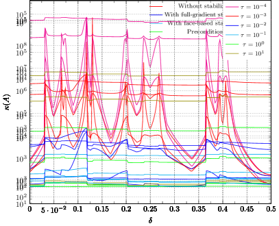
Figure 3: Condition numbers plotted as a function of the position parameter $\delta$.

(a) Bilinear form $a^{1}_{h}(v,w)+\tau j_{h}(v,w)$

(b) Bilinear form $a^{1}_{h}(v,w)+\tau s_{h}(v,w)$

(c) Bilinear form $a^{2}_{h}(v,w)+\tau j_{h}(v,w)$

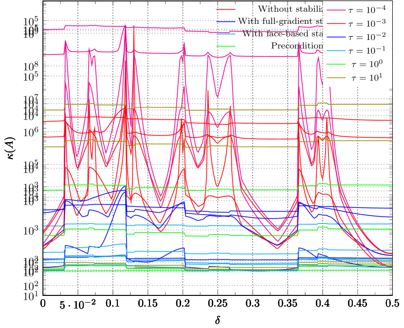
(d) Bilinear form $a^{2}_{h}(v,w)+\tau s_{h}(v,w)$

Figure 4: Condition numbers plotted as a function of the position parameter $\delta$ for different combinations of forms, stabilizations, and penalty parameters.

References

• Burman et al. [2015a] E. Burman, S. Claus, P. Hansbo, M.G. Larson, and A. Massing. CutFEM: discretizing geometry and partial differential equations. Internat. J. Numer. Meth. Engng, 104(7):472–501, 2015a.
• Burman et al. [2015b] E. Burman, P. Hansbo, and M. G. Larson. A stabilized cut finite element method for partial differential equations on surfaces: The Laplace–Beltrami operator. Comput. Methods Appl. Mech. Engrg., 285:188–207, 2015b.
• Burman et al. [2015c] E. Burman, P. Hansbo, M. G. Larson, and A. Massing. A Cut Discontinuous Galerkin Method for the Laplace-Beltrami Operator. Accepted for publication in IMA J. Num. Anal., available as arXiv preprint arXiv:1507.05835, 2015c.
• Burman et al. [2015d] E. Burman, P. Hansbo, M.G. Larson, and S. Zahedi. Cut finite element methods for coupled bulk-surface problems. Numer. Math., 2015d. doi: 10.1007/s00211-015-0744-3.
• Burman et al. [2016] E. Burman, P. Hansbo, M. G. Larson, and S. Zahedi. Stabilized cut finite element methods for convection problems on surfaces. Submitted for publication, available as arXiv preprint arXiv:1511.02340, 2016.
• Chernyshenko and Olshanskii [2015] A. Y. Chernyshenko and M. A. Olshanskii. An adaptive octree finite element method for PDEs posed on surfaces. Comput. Methods Appl. Mech. Engrg., 291:146–172, August 2015.
• Deckelnick et al. [2014] K. Deckelnick, C. M. Elliott, and T. Ranner. Unfitted finite element methods using bulk meshes for surface partial differential equations. SIAM J. Numer. Anal., 52(4):2137–2162, 2014.
• Demlow and Olshanskii [2012] A. Demlow and M. A. A Olshanskii. An adaptive surface finite element method based on volume meshes. SIAM J. Numer. Anal., 50(3):1624–1647, 2012.
• Dziuk [1988] G. Dziuk. Finite elements for the Beltrami operator on arbitrary surfaces. In Partial differential equations and calculus of variations, volume 1357 of Lecture Notes in Math., pages 142–155. Springer, Berlin, 1988.
• Dziuk and Elliott [2013] G. Dziuk and C. M. Elliott. Finite element methods for surface PDEs. Acta Numer., 22:289–396, 2013.
• Ern and Guermond [2006] A. Ern and J. L. Guermond. Evaluation of the condition number in linear systems arising in finite element approximations. ESAIM: Math. Model. Num. Anal., 40(1):29–48, 2006.
• Evans and Gariepy [1992] L. C. Evans and R. F. Gariepy. Measure Theory and Fine Properties of Functions. Studies in Advanced Mathematics. CRC Press, Boca Raton, FL, 1992.
• Gilbarg and Trudinger [2001] D. Gilbarg and N. S. Trudinger. Elliptic Partial Differential Equations of Second Order. Classics in Mathematics. Springer-Verlag, Berlin, 2001.
• Gross et al. [2015] S. Gross, M. A. Olshanskii, and A. Reusken. A trace finite element method for a class of coupled bulk-interface transport problems. ESAIM: Math. Model. Numer. Anal., 49(5):1303–1330, 2015.
• Hansbo et al. [2003] A. Hansbo, P. Hansbo, and M. G. Larson. A finite element method on composite grids based on Nitsche’s method. ESAIM: Math. Model. Num. Anal., 37(3):495–514, 2003.
• Hansbo et al. [2015a] P. Hansbo, M. G. Larson, and S. Zahedi. Characteristic cut finite element methods for convection–diffusion problems on time dependent surfaces. Comput. Methods Appl. Mech. Engrg., 293:431–461, 2015a.
• Hansbo et al. [2015b] P. Hansbo, M.G. Larson, and S. Zahedi. A cut finite element method for coupled bulk-surface problems on time-dependent domains. arXiv:1502.07142v2.pdf, 2015b. To appear in Comput. Methods Appl. Mech. Engrg.
• Massing et al. [2014] A. Massing, M. G. Larson, A. Logg, and M. E. Rognes. A stabilized Nitsche overlapping mesh method for the Stokes problem. Numer. Math., 128(1):73–101, 2014.
• Olshanskii and Reusken [2010] M. A. Olshanskii and A. Reusken. A finite element method for surface PDEs: matrix properties. Numer. Math., 114(3):491–520, 2010.
• Olshanskii and Reusken [2014] M. A. Olshanskii and A. Reusken. Error analysis of a space-time finite element method for solving PDEs on evolving surfaces. SIAM J. Numer. Anal., 52(4):2092–2120, 2014.
• Olshanskii et al. [2009] M. A. Olshanskii, A. Reusken, and J. Grande. A finite element method for elliptic equations on surfaces. SIAM J. Numer. Anal., 47(5):3339–3358, 2009.
• Olshanskii et al. [2014a] M. A. Olshanskii, A. Reusken, and X. Xu. A stabilized finite element method for advection–diffusion equations on surfaces. IMA J. Numer. Anal., 34(2):732–758, 2014a.
• Olshanskii et al. [2014b] M. A. Olshanskii, A. Reusken, and X. Xu. An Eulerian space-time finite element method for diffusion problems on evolving surfaces. SIAM J. Numer. Anal., 52(3):1354–1377, 2014b.
• Reusken [2013] A. Reusken. A finite element level set redistancing method based on gradient recovery. SIAM Journal on Numerical Analysis, 51(5):2723–2745, 2013.
• Reusken [2015] A. Reusken. Analysis of trace finite element methods for surface partial differential equations. IMA Journal of Numerical Analysis, 35(4):1568–1590, 2015.
• Scott and Zhang [1990] R. Scott and S. Zhang. Finite element interpolation of nonsmooth functions satisfying boundary conditions. Math. Comp., 54(190):483–493, 1990.