Reply to “Comment on ‘Breakdown of the expansion of finite-size corrections to the hydrogen Lamb shift in moments of charge distribution’ ”

Abstract

To comply with the critique of the Comment [J. Arrington, arXiv:1602.01461], we consider another modification of the proton electric form factor, which resolves the “proton-radius puzzle”. The proposed modification satisfies all the consistency criteria put forward in the Comment, and yet has a similar impact on the puzzle as that of the original paper. Contrary to the concluding statement of the Comment, it is not difficult to find an ad hoc modification of the form factor at low $Q$ that resolves the discrepancy and is consistent with analyticity constraints. We emphasize once again that we do not consider such an ad hoc modification of the proton form factor to be a solution of the puzzle until a physical mechanism for it is found.

The formalism developed in Ref. Hagelstein:2015yma was illustrated by a modification of the proton electric form factor (FF), $G_{E}$, which could reconcile the discrepancy in the various proton radius extractions. As is correctly pointed out in the Comment Arrington:2015 , this modification is inconsistent with the analyticity constraints. The latter require that all the singularities of $G_{E}(Q^{2})$ lie on the negative $Q^{2}$–axis, whereas the modification has a pole near the positive axis resulting in a resonance-like structure, as seen in Fig. 1 (red dashed curve), as well as in the figure of the Comment.

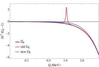
Figure 1: $G_{E}(Q^{2})-1$ and $\overline{G}_{E}(Q^{2})-1$ as a function of $Q$. The solid black curve shows the empirical FF from Ref. Arrington:2006hm . The dashed red curve shows the modified FF from Ref. Hagelstein:2015yma . The dotted blue curve is the modified FF of this work.

Here we present a modified $G_{E}$, shown in Fig. 1 (blue dotted curve), that complies with the consistency requirements put forward in the Comment, and is yet resolving the discrepancy in exactly the same way as described in the original paper. The rest of this Reply can be viewed as the revised Sec. III of Ref. Hagelstein:2015yma :

III. RESOLVING THE PUZZLE

We assume the electric FF to separate into a smooth ($\overline{G}_{E}$) and a nonsmooth part ($\widetilde{G}_{E}$), such that,

$$G_{E}(Q^{2})=\overline{G}_{E}(Q^{2})+\widetilde{G}_{E}(Q^{2}).$$ (20)

For the smooth part we shall take a well-known parametrization which fits the $ep$ data, while for the nonsmooth one we take

$$\widetilde{G}_{E}(Q^{2})=\frac{A\,Q_{0}^{2}\,Q^{2}\left[Q^{2}+\epsilon^{2}\right]}{\left[Q_{0}^{2}+Q^{2}\right]^{4}},$$ (21)

where $A$, $\epsilon$ and $Q_{0}$ are real parameters. The poles of this function are at negative $Q^{2}$ (timelike region) and hence it obeys the analyticity constraint.

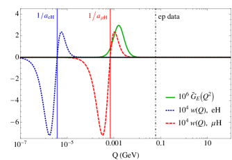
Figure 2: The correction, $\widetilde{G}_{E}(Q^{2})$, for $Q_{0}=1.6$ MeV, $A=1.2\times 10^{-4}$ MeV² and $\epsilon=0.143$ MeV (solid green), and the weighting function, $w(Q)$, for $e$H (blue dotted) and $\mu$H (red dashed) as functions of $Q$. The dash-dotted line indicates the onset of electron-proton scattering data.

According to Fig. 2, in order to make a maximal impact on the puzzle, the fluctuation $\widetilde{G}_{E}$ must be located at the extremi of $w(Q)$ in Eq. (19a) around either the $e$H or $\mu$H inverse Bohr radius. Here we shall only consider the latter case and set one of the position parameters to the MeV scale:

$$Q_{0}=1.6\,\mbox{MeV}.$$ (22)

This choice conditions the choice of the smooth part $\bar{G}_{E}$, in case one wants to solve the puzzle. Indeed, since with this $Q_{0}$ the nonsmooth part affects mostly the $\mu$H result, the smooth part must have a radius consistent with the $e$H value. We therefore adopt the chain-fraction fit of Arrington and Sick Arrington:2006hm :

$$\overline{G}_{E}(Q^{2})=\frac{1}{1+\frac{3.478\,Q^{2}}{1-\frac{0.140\,Q^{2}}{1-\frac{1.311\,Q^{2}}{1+\frac{1.128\,Q^{2}}{1-0.233\,Q^{2}}}}}}.$$ (23)

Fixing $Q_{0}$, the other two parameters of $\widetilde{G}_{E}$, $A$, and $\epsilon$, are fitted by requiring our FF to yield the empirical Lamb shift contribution, in both normal and muonic hydrogen, i.e.:

$$E^{\mathrm{FF}(exp.)}_{2P-2S}(e\mathrm{H})=-0.620(11)\,\mbox{neV},$$ (24a)

$$E^{\mathrm{FF}(exp.)}_{2P-2S}(\mu\mathrm{H})=-3650(2)\,\mbox{$\upmu$eV}.$$ (24b)

Note that these are not the experimental Lamb shifts, but only the finite-size contributions, described by Eqs. (2) and (4), with the corresponding empirical values for the radii. In the $e$H case we have taken the CODATA value of the proton radius, Eq. (3a), which is obtained as an weighted average over several hydrogen spectroscopy measurements, and $R_{E(2)}=2.78(14)$ fm Borie:2012zz . In the $\mu$H case we have taken the values from Ref. Antognini:2013rsa , hence Eq. (3b) for the radius and the same as the above value for $R_{E(2)}$.

Figure 3 shows at which $A$ and $\epsilon$ our FF complies with either the $e$H (blue dot-dashed curve) or $\mu$H (red solid curve) Lamb shift. For $A=1.2\times 10^{-4}$ MeV² and $\epsilon=0.143$ MeV, our FF describes them both, thus resolving the puzzle (the description of the $ep$ data by $\bar{G}_{E}$ is not affected by the addition of $\widetilde{G}_{E}$).

Figure 2 shows the fitted $\widetilde{G}_{E}$, and the weighting function (17) for $e$H and $\mu$H. The modification thus enhances the FF in the region below the onset of $ep$ data ($Q<63$ MeV). The overlap between the correction and the positive contribution of the $\mu$H weighting function is clearly dominating, resulting in the desired matching to the experimental Lamb shifts given in Eq. (24).

We emphasize that the magnitude of the change in the FF is extremely tiny,

$$\big{|}\widetilde{G}_{E}/\,\overline{G}_{E}\big{|}<3\times 10^{-6},$$ (25)

for any positive $Q^{2}$. The Comment suggests that a comparison of our correction to the deviation of the FF from unity is more fair. For our newly proposed $\widetilde{G}_{E}$, we find this ratio to be:

$$\big{|}\widetilde{G}_{E}/\,(\overline{G}_{E}-1)\big{|}<0.57\,,$$

which does not seem unreasonable either. Furthermore, our new FF modification satisfies another criteria put forward in the Comment, namely: $G_{E}(Q^{2})<1$ for $Q^{2}>0$.

Nevertheless, the modification obviously has a profound effect on the $\mu$H Lamb shift. Its effect on the second and third moments is given by:

$$\widetilde{\langle r^{2}\rangle}_{E} \equiv -6\frac{\mathrm{d}}{\mathrm{d}Q^{2}}\widetilde{G}_{E}(Q^{2})\Big{|}_{Q^{2}=0}=-\frac{6A\epsilon^{2}}{Q_{0}^{6}},\quad$$ (26)

$$\widetilde{\langle r^{3}\rangle}_{E} \equiv \frac{48}{\pi}\int_{0}^{\infty}\!\frac{\mathrm{d}Q}{Q^{4}}\,\left\{\widetilde{G}_{E}(Q^{2})+\mbox{$\frac{1}{6}$}\widetilde{\langle r^{2}\rangle}_{E}Q^{2}\right\},$$ (27)

$$= 15A(Q_{0}^{2}-7\epsilon^{2})/2Q_{0}^{7}.$$

The numerical values of these moments, together with their “would be” effect on the Lamb shift and the non-expanded Lamb result, are given in Table 1. One can see that the expansion in moments breaks down for the the modified FF contribution to $\mu$H.

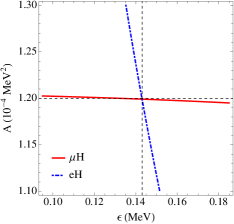
Figure 3: Parameters of $\widetilde{G}_{E}$ for which the $e$H and $\mu$H Lamb shifts of Eq. (24) are reproduced. For fixed $Q_{0}=1.6$ MeV, we chose $A=1.2\times 10^{-4}$ MeV² and $\epsilon=0.143$ MeV, as indicated by the dashed lines.

Table 1: Lamb shift and moments corresponding to our model FF, with $Q_{0}=1.6$ MeV, $A=1.2\times 10^{-4}$ MeV² and $\epsilon=0.143$ MeV.

	Eq.	$\overline{G}_{E}$	$\widetilde{G}_{E}$	$G_{E}$
$\langle r^{2}\rangle_{E}\,[\mbox{fm}^{2}]$	(6a)	$(0.9014)^{2}$	$-(0.1849)^{2}$	$(0.8823)^{2}$
$\langle r^{3}\rangle_{E}\,[\mbox{fm}^{3}]$	(12)	$(1.052)^{3}$	$(8.539)^{3}$	$(8.544)^{3}$
Lamb-shift, expanded	(11)
$E_{2P-2S}^{\mathrm{FF}(1)}(e\mathrm{H})[\text{neV}]$		$-0.6569$	$0.0371$	$-0.6198$
$E_{2P-2S}^{\mathrm{FF}(1)}(\mu\mathrm{H})[\upmu\text{eV}]$		$-4202$	$11542$	$7340$
Lamb-shift, exact	(19a)
$E_{2P-2S}^{\mathrm{FF}(1)}(e\mathrm{H})[\text{neV}]$		$-0.6569$	$0.0370$	$-0.6200$
$E_{2P-2S}^{\mathrm{FF}(1)}(\mu\mathrm{H})[\upmu\text{eV}]$		$-4202$	$552$	$-3650$

In conclusion, we have reworked the low-$Q$ modification of the empirical proton FF $G_{E}$ such that it complies with the criteria put forward in the Comment Arrington:2015 . The original (‘old’) and the reworked (‘new’) modifications are shown in Fig. 1, together with the unmodified form. The old and new modification are quite different, yet they both allow to describe the $e$H and $\mu$H Lamb shift simultaneously, while maintaining the agreement with the $ep$ scattering data. The new modification looks much more reasonable from the standpoint of the Comment. However, we emphasize once more that this is not a proposal for the solution of the puzzle — not until a physical mechanism for this effect is found. For a current update on the status of the proton-radius puzzle, see (Hagelstein:2015egb, , Sec. 7) and references therein.

References

- (1) F. Hagelstein and V. Pascalutsa, Breakdown of the expansion of finite-size corrections to the hydrogen Lamb shift in moments of charge distribution, Phys. Rev. A 91, 040502 (2015).
- (2) J. Arrington, Comment on “Breakdown of the expansion of finite-size corrections to the hydrogen Lamb shift in moments of charge distribution”, arXiv:1602.01461 [hep-ph] (to appear in Phys. Rev. A).
- (3) J. Arrington and I. Sick, Precise determination of low-Q nucleon electromagnetic form factors and their impact on parity-violating e-p elastic scattering, Phys. Rev. C 76, 035201 (2007).
- (4) E. Borie, Lamb shift in light muonic atoms: Revisited, Annals Phys. 327, 733 (2012).
- (5) A. Antognini, F. Kottmann, F. Biraben, P. Indelicato, F. Nez and R. Pohl, Theory of the 2S-2P Lamb shift and 2S hyperfine splitting in muonic hydrogen, Annals Phys. 331, 127 (2013).
- (6) F. Hagelstein, R. Miskimen and V. Pascalutsa, Nucleon polarizabilities: From Compton scattering to hydrogen atom, Prog. Part. Nucl. Phys., doi:10.1016/j.ppnp.2015.12.001 (arXiv:1512.03765 [nucl-th]).