Next-to-leading power threshold logarithms: a status report

Abstract:

There is ample evidence, dating as far back as Low’s theorem, that the universality of soft emissions extends beyond leading power in the soft energy. This universality can, in principle, be exploited to generalise the formalism of threshold resummations beyond leading power in the threshold variable. In the past years, several phenomenological approaches have been partially successful in performing such a resummation. Here, we briefly review some recent developments which pave the way to a solution of this problem, at least for electroweak annihilation processes.

1 Introduction

Standard Model cross sections of interest for LHC often involve many different physical scales, including for example Mandelstam invariants, heavy particle masses and jet masses. Since the Standard Model is a renormalisable gauge theory, perturbative expressions for these cross section always involve powers of logarithms of ratios of these scales. When some of the scales are disparate, the logarithms are large, and they often spoil the reliability of perturbation theory in phenomenologically relevant kinematic regions. In many cases, these logarithms are associated with underlying singularities of scattering amplitudes, and in particular they often appear as finite remainders after the cancellation of divergences arising at the edges of phase space. As a consequence, such logarithms have a universal nature, in the sense that they do not depend on the details of the hard scattering process at hand. They can then be computed once and for all, and often formally summed up to all orders in perturbation theory, yielding improved predictions for physical observables which can be applied to more extreme configurations. Well-known examples of this ‘resummation’ technology are given by the renormalisation group, by perturbative Reggeization, and by Sudakov resummation.

In this contribution, we will be concerned with a specific class of these logarithms, arising when a partonic cross section is evaluated in the vicinity of a physical threshold for the production of a selected final state. A slightly unconventional way to define these ‘threshold logarithms’ is the following: they are those that arise in distributions which, at Born level, are localised at the threshold (in other words, the Born distribution is a delta function). This definition thus includes $p_{t}$ logarithms arising, say, in the Drell-Yan or Higgs $p_{t}$ distributions, as well as conventional Sudakov logarithms in the inclusive cross sections for electroweak annihilation processes, DIS, and event shapes in electron-positron annihilation.

In all these cases, one can define a ”threshold variable” $\xi$, such that the Born cross section is proportional to $\delta(\xi)$. Loop corrections generically take the form

$$\frac{d\sigma}{d\xi}\,=\,\sum_{n=0}^{\infty}\left(\frac{\alpha_{s}}{\pi}\right)^{n}\,\sum_{m=0}^{2n-1}\left[c_{nm}^{(-1)}\left(\frac{\log^{m}\xi}{\xi}\right)_{+}+\,c_{nm}^{(\delta)}\,\delta(\xi)\,+\,c_{nm}^{(0)}\,\log^{m}\xi\,+\,\ldots\right]\,,$$ (1)

where the ‘plus distribution’ notation is used here generically to indicate that one must include virtual corrections in order for the first set of terms to be integrable. The logarithmic terms with coefficients given by $c_{nm}^{(-1)}$ are the conventional Sudakov logarithms, closely connected to infrared and collinear divergences of the relevant amplitudes. Their resummation has been well understood for many years, and is routinely applied, to high logarithmic accuracy, for a wide range of observables. In the present context, we refer to these terms as leading-power (LP) threshold logarithms. The second set of terms, with coefficients given by $c_{nm}^{(\delta)}$, arises from finite virtual corrections and from remainders of phase space integrations after the cancellation of IR and collinear poles. Interestingly, as we will briefly review below, for cross sections that are purely electroweak at tree level these terms can also be studied to all orders in perturbation theory, albeit with a lesser degree of control as compared with LP logarithms. Finally, the last set of terms in Eq. (1), with coefficients given by $c_{nm}^{(0)}$, is the main subject of this contribution: these terms are integrable, but they can still give significant contributions to the cross section, order by order in perturbation theory, when $\xi$ is small. We refer to these terms as next-to-leading-power (NLP) threshold logarithms. Over the years, an increasing body of evidence has accumulated, suggesting that NLP logarithms can be organised to all orders in perturbation theory, similarly to what happens at LP. Our goal here is to briefly review this body of evidence, and then summarise some very recent results which were presented in detail in Refs. [1, 2].

2 Gathering evidence

Beyond LP threshold logarithms, the first interesting contributions to the cross section are those which are localised at the threshold, specified by the coefficients $c_{nm}^{(\delta)}$ in Eq. (1). In dimensional regularisation, and for processes which are electroweak at tree level, all these terms are naturally organised in exponential form, as a consequence of the evolution equations obeyed by the various factors composing the partonic cross section. The first observation in this direction dates back to [4], and has been successively refined, extended and revisited in [5, 6, 7]. Following the reasoning of [6], and using the Drell-Yan process as an example, one may simply note that the partonic cross section for quark-initiated Drell-Yan near threshold obeys the (Mellin space) factorisation theorem [5]

$$\omega(N,\epsilon)\,=\,\left|\Gamma\left(Q^{2},\epsilon\right)\right|^{2}\,\left[\psi_{R}(N,\epsilon)\right]^{2}\,U_{R}(N,\epsilon)+{\cal O}\left(\frac{1}{N}\right)\,,$$ (2)

where $\Gamma$ is the quark form factor, and $\psi_{R}$ and $U_{R}$ are responsible respectively for collinear and soft real radiation into the final state. In Eq. (2) real and virtual correction are treated separately: this is possible only because each factor obeys evolution equations which can be solved in exponential form, with trivial boundary conditions in dimensional regularisation. Infrared divergences cancel between the real emission function $U_{R}$ and the virtual form factor, while collinear divergences remain in the parton distribution $\psi_{R}$, in factorised form. To construct the finite partonic Drell-Yan cross section in Mellin space, in the ${\overline{MS}}$ scheme, it is now sufficient to divide Eq. (2) by the square of the ${\overline{MS}}$ parton distribution $\phi_{\overline{MS}}$, which can also be written as the product of a virtual factor times a real emission factor. One is led to the expression

$$\widehat{\omega}_{\overline{MS}}(N)\,=\,\left(\frac{\left|\Gamma\left(Q^{2},\epsilon\right)\right|^{2}}{\left[\phi_{V}(\epsilon)\right]^{2}}\right)\,\left(\frac{\left[\psi_{R}(N,\epsilon)\right]^{2}\,U_{R}(N,\epsilon)}{\left[\phi_{R}(N,\epsilon)\right]^{2}}\right)+{\cal O}\left(\frac{1}{N}\right)\,.$$ (3)

Since each factor in Eq. (3) exponentiates, and the factorisation is accurate up to NLP corrections, it follows that constant terms in Mellin space (corresponding to localised terms in momentum space) are naturally defined in the exponent. Clearly, the predictive power of this statement is limited: when exponentiating logarithms, a finite-order calculation makes an exact prediction for a set of infinite towers of logarithmic corrections to all orders in perturbation theory; constants, on the other hand, cannot be categorised by parametric enhancements: therefore, at order $n$, they receive contributions both from the exponentiation of lower orders and from terms genuinely arising at order $n$. This not withstanding, it is certainly legitimate to use exponentiation at least as a tool to estimate the size of higher-order localised corrections.

At NLP level, the first historical bit of evidence for the universality of logarithmic corrections is Low’s theorem [8], to be reviewed in the next section. It is however non-trivial to make use of Low’s theorem to construct a resummation formalism. A more immediately applicable proposal was made in [9], building upon an empirical observation arising from the three-loop calculation of Ref. [10]. The central physical input of [9] is reciprocity, the idea that the evolution kernels for parton splitting and fragmentation should be simply related by analytic continuation. This idea can be realised by making use of a modified evolution equation, the DMS equation, which can be written as

$$\mu^{2}\frac{\partial}{\partial\mu^{2}}\,\psi(x,\mu^{2})\,=\,\int_{x}^{1}\frac{dz}{z}\,\psi\left(\frac{x}{z},z^{\sigma}\mu^{2}\right){\cal P}\left(z,\alpha_{s}\left(\frac{\mu^{2}}{z}\right)\right)\,,$$ (4)

where $\sigma=+1$ for space-like evolution of parton densities, and $\sigma=-1$ for time-like evolution of fragmentation functions. Ref. [9] argues that, in a renormalisation scheme where the coupling is defined to equal the light-like cusp anomalous dimension, the universal kernel ${\cal P}$ has the remarkable property of having no corrections at NLP in $(1-z)$. In other words, one may write

$${\cal P}\left(z,\alpha_{s}\right)\,=\,\frac{A(\alpha_{s})}{(1-z)_{+}}+B_{\delta}(\alpha_{s})\delta(1-z)+{\cal O}(1-z)\,,$$ (5)

a relation which is verified up to three loops in QCD. Clearly, Eq. (4) cannot be solved as easily as the ordinary DGLAP equation, since it is not diagonalised by a Mellin transform. It is however possible to solve it recursively, order by order in perturbation theory. Proceeding in this way, and using Eq. (5), one can map DMS evolution into ordinary DGLAP evolution, with a modified kernel such that higher-order coefficients of NLP contributions are determined by lower-order coefficients of the anomalous dimensions $A(\alpha_{s})$ and $B_{\delta}(\alpha_{s})$, explaining and generalising the observation of Ref. [10].

These insights can easily be combined to construct an improved threshold resummation formula, including in the perturbative exponent a subset of NLP logarithms, as well as contributions localised at threshold. This was done in Ref. [11], where the following expression was proposed for the Drell-Yan cross section

$$\ln\Big{[}\widehat{\omega}(N)\Big{]} = {\cal F}_{\rm DY}\left(\alpha_{s}(Q^{2})\right)+\int_{0}^{1}\,dz\,z^{N-1}\,\Bigg{\{}\frac{1}{1-z}\,D\left[\alpha_{s}\left(\frac{(1-z)^{2}Q^{2}}{z}\right)\right]$$ (6)

$$+\,\,2\,\int_{Q^{2}}^{(1-z)^{2}Q^{2}/z}\,\frac{dq^{2}}{q^{2}}\,P_{s}\Big{[}z,\alpha_{s}(q^{2})\Big{]}\Bigg{\}}_{+}\,.$$

Eq. (6) improves upon standard LP threshold resummation in three ways: first, contributions localized at threshold are included in the exponent, collected in the function ${\cal F}_{DY}(\alpha_{s})$; second, phase space limits for soft radiation are evaluated to higher accuracy in $(1-z)$, both in the argument of the coupling in the soft function $D(\alpha_{s})$ and in the limit of integration; third, in the leading term the cusp anomalous dimension is replaced by the DMS-improved splitting function $P_{s}$. Explicit comparison of Eq. (6) with finite order results at two and three loops shows that leading and next-to-leading NLP logarithms at higher orders are predicted with remarkable accuracy, based on lower order results: for example, leading NLP logarithms at two loops can be generated by the simple substitution $2/(1-z)\to 2z/(1-z)$ in the cusp term, as was noticed already in Ref. [13]. Further subleading NLP logarithms, however, are predicted with decreasing accuracy, and it is clear that a more systematic approach is necessary in order to achieve a reliable and complete resummation. Steps towards such an approach are described in the next two sections.

3 Towards systematics

Over the past several years, a number of approaches have been developed to improve our understanding of NLP logarithms in hadronic cross sections. The literature is vast and cannot be reviewed here, but, to mention the most recent delopments, the physical kernel method developed by Moch and Vogt [14] has been recently applied to the Higgs production cross section in [15], and Soft-Collinear Effective Theory has been applied to this problem in [16, 17]. In a massless theory, such as perturbative QCD in most applications, the challenge of constructing a general formalism is dual: first, one must study how the formalism of soft gluon factorisation and exponentiation generalises beyond leading power; then one must include in the picture (next-to-) collinear configurations, which may (and do) interfere with the soft expansion.

The task of extending the well-known soft factorisation and exponentiation theorems beyond leading power was first tackled in [18], using a path integral formalism. Neglecting collinear problems, and using techniques similar to world-line methods, it is easy to see how the eikonal approximation arises in this context. The replica trick often used in statistical field theory then leads to exponentiation at eikonal level. These methods can be extended to next-to-leading power in the soft energy, sometimes called Next-to-Eikonal (NE): the result is that a large set of contributions to scattering amplitudes factorise and exponentiate, and the exponent of the next-to-soft factor can be directly computed in terms of NE Feynman rules. A non-factorizable remainder survives, which in this context is partly associated with translations of the relevant Wilson lines. Using Ward identities, this setup can be transparently mapped back to Low’s theorem in the simple case of photon emission. The same conclusion can be confirmed from a purely diagrammatic point of view, which was pursued in Ref. [19]. With this method, the problem is straightforward in principle, but requires a very intricate combinatorial analysis. The starting point is the expansion of the propagator of the particle carrying the hard momentum $p$, and emitting the soft gluon, in powers of the soft gluon momentum $k$. For a massless spin one-half emitter, one writes

$$\frac{p\hskip-4.49997pt/+k\hskip-4.49997pt/}{2p\cdot k+k^{2}}\gamma^{\mu}u(p)\,=\,\left[\frac{p^{\mu}}{p\cdot k}-k^{2}\frac{p^{\mu}}{2\left(p\cdot k\right)^{2}}+\frac{k\hskip-4.49997pt/\gamma^{\mu}}{2p\cdot k}\right]u(p)\,+\,{\cal O}(k)\,,$$ (7)

where one recognises the eikonal vertex at leading power in $k$, followed by a spin-independent next-to-soft term, and finally by a spin-dependent contribution. Indeed, it is well-known since Low’s days [20] that the universality (and in particular the spin-independence) of soft emissions breaks down at NLP in the soft energy. At the level of matrix elements, the results of Refs. [18, 19] can be summarised as follows.

In the eikonal approximation, it is well known that soft emissions factorise from matrix elements, and the resulting soft function can be written as a correlator of Wilson lines (see, for example, [21, 22]). Furthermore, it is known that the soft function exponentiates, and the exponent can be directly computed in terms of a subset of the original Feynman diagrams [23, 24]. For a correlator of $n$ Wilson lines, one writes

$$S_{n}\equiv\langle 0|\Phi_{1}\otimes\ldots\otimes\Phi_{n}|0\rangle\,=\,\exp\left(w_{n}\right)\,.$$ (8)

If one then expresses each diagram $D$ contributing to $S_{n}$ as the product of a color factor $C(D)$ and a kinematic factor ${\cal F}(D)$, one finds that $w_{n}$ can be written, order by order in the coupling, as a sum over a subset of the diagrams $D$, organized in structures called webs. Each web is a set of diagrams differing by the order of gluon attachments on the Wilson lines, and computed with modified color factors, according to

$$W\,=\,\sum_{D\in W}\widetilde{C}(D){\cal F}(D)\,=\,\sum_{D,D^{\prime}\in W}C(D^{\prime})\,R\left(D^{\prime},D\right){\cal F}(D)\,,$$ (9)

where $R(D^{\prime},D)$, the web mixing matrix, is a matrix of constant combinatorial coefficients which can be computed recursively [25]. In this language, Refs. [18, 19] show that matrix elements retain a similar structure at NLP. One may formally write

$${\cal M}\,=\,{\cal M}_{0}\,\exp\left[\sum_{D_{E}}\widetilde{C}\left(D_{E}\right){\cal F}\left(D_{E}\right)+\sum_{D_{NE}}\widetilde{C}\left(D_{NE}\right){\cal F}\left(D_{NE}\right)\right]\,+\,{\cal M}_{R}\,+\,{\cal O}\left(NNE\right)\,,$$ (10)

where $D_{E}$ are the diagrams (forming webs) that would appear in the eikonal approximation, while $D_{NE}$ are a set of diagrams constructed with new, next-to-eikonal Feynman rules. As might have been expected, factorisation and exponentiation are incomplete at NLP, and a non-factorisable remainder ${\cal M}_{R}$ survives, which can be computed order by order using Low’s theorem.

Eq. (10), with the appropriate NE Feynman rules, was tested in Ref. [19] by reproducing (at NLP) the two loop results for the double real emission contribution to the Drell-Yan cross section. It became clear, however, that the same technique fails when attempting to compute real-virtual corrections. The reason can be traced to a failure of Low’s theorem for massless particles, which we discuss in the next section.

4 Factorization at NLP level

The original version of Low’s theorem [8], later generalised to particles with spin by Burnett and Kroll [20], was derived for massive particles, and with the soft expansion performed in powers of $E/m$, where $E$ is the soft energy and $m$ the mass of the emitter. Clearly the corresponding derivation does not apply for particles of vanishing mass. In modern language, the problem is that in the massless limit collinear divergences arise, governed by a different physical scale with respect to the hard scale of the process. In dimensional regularization, these divergences generate logarithms of that scale, both at LP and NLP, which cannot be captured by the soft expansion. As an illustration, consider the cut graph displayed in Fig. 1, contributing to the Drell-Yan cross section at two loops: near threshold, gluon $k_{2}$ is always (next-to-) soft, but gluon $k_{1}$ is virtual and its momentum components are unconstrained. When $k_{1}$ is (next-to-) soft, the contributions of this diagram are correctly captured by Eq. (10), but when it is hard and collinear to $p$ it contributes to LP and NLP logarithms at every order in the soft expansion.

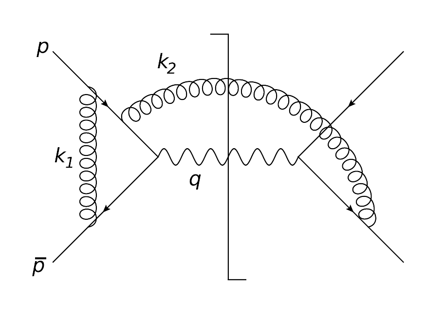
Figure 1: A two-loop cut diagram displaying a collinear singularity affecting Low’s theorem.

This problem was known since early days, and (in the case of QED) it was solved by Del Duca in Ref. [26]. The solution provides a generalization of Low’s theorem (which we refer to as LBKD theorem) valid for soft energies in the range $m^{2}/Q<E<m$, with Q the hard scale of the problem. Clearly, this generalization applies to the massless limit, and it can be adapted to QCD. With minor modifications, the LBKD theorem expresses a hard amplitude with the radiation of an extra soft gluon in terms of the non-radiative amplitude and of two universal jet functions organising the collinear enhancements. We write it as

$${\cal A}^{\mu}(p_{j},k) = \sum_{i=1}^{2}\Bigg{\{}\,q_{i}\left(\frac{(2p_{i}-k)^{\mu}}{2p_{i}\cdot k-k^{2}}+G^{\nu\mu}_{i}\,\frac{\partial}{\partial p_{i}^{\nu}}\right)$$

$$\hskip 28.45274pt+\,G^{\nu\mu}_{i}\left[\frac{J_{\nu}(p_{i},k,n_{i})}{J(p_{i},n_{i})}-q_{i}\,\frac{\partial}{\partial p_{i}^{\nu}}\Big{(}\ln J(p_{i},n_{i})\Big{)}\right]\Bigg{\}}\,{\cal A}(p_{i};p_{j})\,.$$

One easily recognizes in the first line of Eq. (4) the eikonal factor, supplemented with NE corrections (one could, of course, expand the first term in powers of $k$, or set $k^{2}=0$ for on-shell real radiation). The second term on the first line corresponds to Low’s theorem in the absence of collinear enhancements. Indeed, $G_{i}^{\mu\nu}$ is a tensor associated with the hard leg carrying momentum $p_{i}$ and defined by

$$G_{i}^{\mu\nu}\,=\,\eta^{\mu\nu}-\,K_{i}^{\mu\nu}\,;\qquad K_{i}^{\mu\nu}=\frac{(2p_{i}-k)^{\nu}}{2p_{i}\cdot k-k^{2}}\,k^{\mu}\,.$$ (12)

$G_{i}^{\mu\nu}$ satisfies $p_{i}^{\mu}G_{i,\mu\nu}\sim k_{\nu}$, thus suppressing collinear configurations. The second line of Eq. (4) contains the collinear enhancements, collected in the two jet functions $J$ and $J_{\mu}$. The non-radiative jet function $J(p_{i},n_{i})$ is responsible for collinear divergences along the direction $p_{i}$ in the factorised non-radiative amplitude [21]. It is defined by the gauge-invariant matrix element

$$J(p,n)u(p)\,=\,\langle 0|\Phi_{n}\left(0,\infty\right)\psi(0)|p\rangle\,,$$ (13)

with $n^{\mu}$ a reference direction for the Wilson line $\Phi_{n}$, and $\psi$ the quark field. The radiative jet function $J_{\mu}(p_{i},n_{i},k)$, on the other hand, appears for the first time in this context. It is defined by the gauge-invariant matrix element

$$J_{\mu}\left(p,n,k\right)u(p)\,=\,\int d^{d}y\,\,{\rm e}^{-{\rm i}(p-k)\cdot y}\,\left\langle 0\left|T\Big{[}\,\,\Phi_{n}(y,\infty)\,\psi(y)\,j_{\mu}(0)\Big{]}\,\right|p\right\rangle\,,$$ (14)

where $j_{\mu}$ is the quark current. The non-radiative jet function is responsible for the non-factorised, collinearly enhanced next-to-soft emission from the hard parton carrying momentum $p$. It can easily be evaluated at tree-level, with the result

$$J^{\nu(0)}\left(p,n,k\right)\,=\,-\,\frac{p^{\nu}}{p\cdot k}+\frac{k^{\nu}}{2p\cdot k}-\frac{{\rm i}\,k_{\alpha}\Sigma^{\alpha\mu}}{p\cdot k}\,,$$ (15)

where $\Sigma^{\alpha\mu}$ are the spin one-half generators of the Lorentz group.

Eq. (4) is still not fully satisfactory, since it contains residual dependence on the ‘factorisation vectors’ $n_{i}$, which would need to be subtracted or reabsorbed into a suitably defined matching coefficient. For the specific case of processes which are electroweak at tree level (and thus include only two hard colored partons), there is however a simpler solution. Ordinarily, one would take the $n_{i}$’s such that $n_{i}^{2}\neq 0$, in order to avoid spurious collinear divergences in the $n_{i}$ direction. In the case at hand, however, one may observe that the factor in square brackets in the second line of Eq. (4) is renormalization group invariant: indeed, the UV divergences of $J_{\mu}$ cancel those of $J$ in the first term, while the second is UV finite. One may therefore evaluate the square bracket in terms of bare quantities, and at this point it becomes clearly advantageous to pick $n_{i}^{2}=0$, since with that choice $J(p_{i},n_{i})=1$. Finally, one can make a natural and physical choice for the two factorisation vectors: since the only two physical vectors in the problem are $p_{1}$ and $p_{2}$, one may choose $n_{1}=p_{2}$ and $n_{2}=p_{1}$. With massless reference vectors, Eq. (4) takes the considerably simpler form

$${\cal A}^{\mu}(p_{j},k)\,=\,\sum_{i=1}^{2}\left(q_{i}\,\frac{(2p_{i}-k)^{\mu}}{2p_{i}\cdot k-k^{2}}+q_{i}\,G^{\nu\mu}_{i}\frac{\partial}{\partial p_{i}^{\nu}}+G^{\nu\mu}_{i}J_{\nu}(p_{i},k)\right){\cal A}(p_{i};p_{j})\,,$$ (16)

which can be directly used to compare with perturbative data. The radiative jet function for quarks was computed at one loop (for the $C_{F}$ color structure) in [2]. As a non-trivial test of Eqs. (4) and (16), the $C_{F}^{2}$ terms of the two-loop real-virtual contribution to the Drell-Yan K-factor were reproduced, allowing also for a detailed mapping to the method-of-regions calculation of [1]. The calculation is reviewed in [3].

5 Perspective

With Eq. (4), all the conceptual ingredients required to set up a resummation formalism for NLP threshold logarithms, at least for processes with electroweak final states, are in place. The key information embodied in Eq. (10) and in Eq. (4) is that, at the amplitude level, the contributions generating NLP logarithms are universal in nature, and factorise from the radiationless process, at least in the sense that they can be computed by acting on the non-radiative amplitude either multiplicatively or by means of a differential operator. Much technical work, however, remains to be done: first the full non-abelian generalisation of Eq. (4) must be worked out, together with the renormalisation properties of the radiative jet function in generic color representations. Then one must move from amplitudes to cross sections, which will require the phase space analysis of Ref. [19]. At that stage, the ordinary techniques of factorisation and evolution can be employed to construct a complete resummation formula. Finally, the formalism will have to be extended to colored final states, which will involve the treatment of hard next-to-collinear contributions to final state jets. Along the way, a range of phenomenological applications to interesting collider processes will become available, as has been the case for leading-power threshold resummation.

References

- [1] D. Bonocore, E. Laenen, L. Magnea, L. Vernazza and C. D. White, Phys. Lett. B 742 (2015) 375, arXiv:1410.6406 [hep-ph].
- [2] D. Bonocore, E. Laenen, L. Magnea, S. Melville, L. Vernazza and C. D. White, JHEP 1506 (2015) 008, arXiv:1503.05156 [hep-ph].
- [3] D. Bonocore, arXiv:1512.05364 [hep-ph].
- [4] G. Parisi, Phys. Lett. B 90 (1980) 295.
- [5] G. F. Sterman, Nucl. Phys. B 281 (1987) 310.
- [6] T. O. Eynck, E. Laenen and L. Magnea, JHEP 0306 (2003) 057, hep-ph/0305179.
- [7] V. Ahrens, T. Becher, M. Neubert and L. L. Yang, Phys. Rev. D 79 (2009) 033013, arXiv:0808.3008 [hep-ph].
- [8] F. E. Low, Phys. Rev. 110 (1958) 974.
- [9] Y. L. Dokshitzer, G. Marchesini and G. P. Salam, Phys. Lett. B 634 (2006) 504, hep-ph/0511302.
- [10] S. Moch, J. A. M. Vermaseren and A. Vogt, Nucl. Phys. B 688 (2004) 101, hep-ph/0403192.
- [11] E. Laenen, L. Magnea and G. Stavenga, Phys. Lett. B 669 (2008) 173, arXiv:0807.4412 [hep-ph].
- [12] R. D. Ball, M. Bonvini, S. Forte, S. Marzani and G. Ridolfi, Nucl. Phys. B 874 (2013) 746, arXiv:1303.3590 [hep-ph].
- [13] M. Kramer, E. Laenen and M. Spira, Nucl. Phys. B 511 (1998) 523, hep-ph/9611272.
- [14] S. Moch and A. Vogt, JHEP 0911 (2009) 099, arXiv:0909.2124 [hep-ph].
- [15] D. de Florian, J. Mazzitelli, S. Moch and A. Vogt, JHEP 1410 (2014) 176, arXiv:1408.6277 [hep-ph].
- [16] A. J. Larkoski, D. Neill and I. W. Stewart, JHEP 1506 (2015) 077, arXiv:1412.3108 [hep-th].
- [17] D. W. Kolodrubetz, I. Moult and I. W. Stewart, arXiv:1601.02607 [hep-ph].
- [18] E. Laenen, G. Stavenga and C. D. White, JHEP 0903 (2009) 054, arXiv:0811.2067 [hep-ph].
- [19] E. Laenen, L. Magnea, G. Stavenga and C. D. White, JHEP 1101 (2011) 141, arXiv:1010.1860 [hep-ph].
- [20] T. H. Burnett and N. M. Kroll, Phys. Rev. Lett. 20 (1968) 86.
- [21] L. J. Dixon, L. Magnea and G. F. Sterman, JHEP 0808 (2008) 022, arXiv:0805.3515 [hep-ph].
- [22] E. Gardi and L. Magnea, Nuovo Cim. C 32N5-6 (2009) 137, arXiv:0908.3273 [hep-ph].
- [23] E. Gardi, E. Laenen, G. Stavenga and C. D. White, JHEP 1011 (2010) 155, arXiv:1008.0098 [hep-ph].
- [24] A. Mitov, G. Sterman and I. Sung, Phys. Rev. D 82 (2010) 096010, arXiv:1008.0099 [hep-ph].
- [25] E. Gardi and C. D. White, JHEP 1103 (2011) 079, arXiv:1102.0756 [hep-ph].
- [26] V. Del Duca, Nucl. Phys. B 345 (1990) 369.