Hydrodynamics of Suspensions of Passive and Active Rigid Particles:
A Rigid Multiblob Approach

Abstract

We develop a rigid multiblob method for numerically solving the mobility problem for suspensions of passive and active rigid particles of complex shape in Stokes flow in unconfined, partially confined, and fully confined geometries. As in a number of existing methods, we discretize rigid bodies using a collection of minimally-resolved spherical blobs constrained to move as a rigid body, to arrive at a potentially large linear system of equations for the unknown Lagrange multipliers and rigid-body motions. Here we develop a block-diagonal preconditioner for this linear system and show that a standard Krylov solver converges in a modest number of iterations that is essentially independent of the number of particles. Key to the efficiency of the method is a technique for fast computation of the product of the blob-blob mobility matrix and a vector. For unbounded suspensions, we rely on existing analytical expressions for the Rotne-Prager-Yamakawa tensor combined with a fast multipole method (FMM) to obtain linear scaling in the number of particles. For suspensions sedimented against a single no-slip boundary, we use a direct summation on a Graphical Processing Unit (GPU), which gives quadratic asymptotic scaling with the number of particles. For fully confined domains, such as periodic suspensions or suspensions confined in slit and square channels, we extend a recently-developed rigid-body immersed boundary method [“An immersed boundary method for rigid bodies”, B. Kallemov, A. Pal Singh Bhalla, B. E. Griffith, and A. Donev, Communications in Applied Mathematics and Computational Science, 11-1, 79-141, 2016] to suspensions of freely-moving passive or active rigid particles at zero Reynolds number. We demonstrate that the iterative solver for the coupled fluid and rigid body equations converges in a bounded number of iterations regardless of the system size. In our approach, each iteration only requires a few cycles of a geometric multigrid solver for the Poisson equation, and an application of the block-diagonal preconditioner, leading to linear scaling with the number of particles. We optimize a number of parameters in the iterative solvers and apply our method to a variety of benchmark problems to carefully assess the accuracy of the rigid multiblob approach as a function of the resolution. We also model the dynamics of colloidal particles studied in recent experiments, such as passive boomerangs in a slit channel, as well as a pair of non-Brownian active nanorods sedimented against a wall.

I Introduction

The study of the hydrodynamics of colloidal suspensions of passive particles is an old yet still active subject in soft condensed matter physics and chemical engineering. In recent years there has been a growing interest in suspensions of active colloids ActiveSuspensions , which exhibit rich collective behaviors quite distinct from those of passive suspensions. There is a growing number of computational methods for modeling active suspensions IrreducibleActiveFlows_PRL ; MicroSwimmers_Lushi ; SquirmersFCM ; StokesianDynamics_Rigid ; ActiveFilaments_Adhikari ; ActiveFilaments_RPY ; BoundaryIntegralGalerkin ; Galerkin_Wall_Spheres , which are typically built upon well-developed techniques for passive suspensions in steady Stokes flow, i.e., at zero Reynolds number. Since active particles typically have metallic subcomponents, they are often significantly denser than the solvent and sediment toward the bottom wall, making it necessary to address confinement and implement non-periodic boundary conditions in any method aimed at simulating experimentally-relevant configurations. Furthermore, since collective motions seen in active suspensions involve large numbers of particles, and since hydrodynamic interactions among particles decay slowly like the inverse of the distance, it is crucial to develop methods that can capture long-ranged hydrodynamic effects, yet still scale to tens or hundreds of thousands of particles.

For suspensions of passive particles the methods of Brownian BrownianDynamics_DNA ; BrownianDynamics_OrderN and Stokesian dynamics BrownianDynamics_OrderNlogN ; StokesianDynamics_Wall have dominated in chemical engineering, and related techniques have been used in biochemical engineering HYDROLIB ; SphereConglomerate ; HYDROPRO ; HYDROPRO_Globular ; Multiblob_RPY_Rotation . These methods simulate the overdamped (diffusive) dynamics of the particles by using Green’s functions for steady Stokes flow to capture the effect of the fluid. While this sort of implicit solvent approach works very well in many situations, it has several notable technical difficulties: achieving near linear scaling for many-particle systems is technically challenging, handling non-trivial boundary conditions (bounded systems) is complicated and has to be done on a case-by-case basis BrownianDynamics_DNA2 ; StokesianDynamics_Wall ; StokesianDynamics_Slit ; StokesianDynamics_Confined ; BD_LB_Comparison ; RegularizedStokeslets_Walls ; RegularizedStokeslets_Periodic ; SpectralEwald_Stokes ; BoundaryIntegral_Wall ; BoundaryIntegral_Periodic3D ; BrownianDynamics_OrderN2 , generalizations to non-spherical (and in particular complex) particle shapes is difficult, and including thermal fluctuations is non-trivial due to the need to obtain stochastic increments with the desired covariance. In this work we develop relatively low-accuracy but flexible and simple rigid multiblob methods that address these difficulties. Our approach builds heavily on a number of existing techniques, combining elements from several distinct but related methods. We extensively test the proposed methods and study their accuracy and performance on a number of test problems.

The continuum formulation of the Stokes equations with suitable boundary conditions on the surfaces of a collection of rigid particles is well-known and summarized in more detail in Appendix A. Due to the linearity of the Stokes equations, there is an affine mapping from the applied forces $\boldsymbol{f}$ and torques $\boldsymbol{\tau}$ and any specified apparent slip velocity due to active boundary layers $\breve{\boldsymbol{u}},$ to the resulting particle motion given by the linear velocities $\boldsymbol{u}$ and the angular velocities $\boldsymbol{\omega}$. Specifically,

$$\left[\begin{array}[]{c}\boldsymbol{u}\\ \boldsymbol{\omega}\end{array}\right]=\boldsymbol{\mathcal{N}}\left[\begin{array}[]{c}\boldsymbol{f}\\ \boldsymbol{\tau}\end{array}\right]-\breve{\boldsymbol{\mathcal{N}}}\breve{\boldsymbol{u}},$$ (1)

where $\boldsymbol{\mathcal{N}}$ is the mobility matrix, and $\breve{\boldsymbol{\mathcal{N}}}$ is an active mobility linear operator. The mobility problem consists of computing the rigid-body motion given the applied forces and torques and apparent slip. The inverse of this problem is the resistance problem, which computes the forces and torques on the body given a specified motion of the body and active slip. Solving the mobility problem is a key component of any numerical method for modeling the deterministic or fluctuating (Brownian) dynamics of the particles.

In this paper we develop a mobility solver for suspensions of rigid particles immersed in viscous fluid, specifically, we develop novel preconditioners for iterative solvers for the unknown motions of the rigid bodies, given the applied external forces and torques as well as active apparent slip on the surface of the particles. As we discuss in more detail in the body of the paper, our formulation can readily solve the resistance problem; however, our iterative solvers will prove to be more scalable for mobility computations (which are of primary interest) than for resistance computations. Key to the success of our iterative solvers is the idea that instead of eliminating variables using exact Schur complements and solving a reduced system iteratively, as done in the majority of existing methods RigidMultiblobs_Swan ; StokesianDynamics_Rigid ; FluctuatingFCM_DC , one should instead iteratively solve an extended system that includes all of the variables. This has the key advantage that the matrix-vector product becomes an efficient direct calculation, and the Schur complement can be computed only approximately and used to construct an effective preconditioner.

Like many other authors, we construct rigid bodies of essentially arbitrary shape as a collection of rigidly-connected collection of “blobs” or “beads” forming a composite object RigidMultiblobs_Swan that we will refer to as a rigid multiblob. The hydrodynamic interactions between blobs are represented using a Rotne-Prager tensor generalized to the desired domain geometry (boundary conditions) RPY_Shear_Wall , specifically, we use the the Rotne-Prager-Yamakawa (RPY) tensor RotnePrager for an unbounded domain, and the Rotne-Prager-Blake (RPB) tensor StokesianDynamics_Wall for a half-space domain. In Section II we describe how to obtain the hydrodynamic coupling between a large collection of rigid multiblobs by solving a large linear system for Lagrange multipliers enforcing the rigidity. A key contribution of our work is to develop an indefinite saddle-point preconditioner for iterative solution of the resulting linear system. This preconditioner is based on a block-diagonal approximation of the blob-blob mobility matrix, in which all hydrodynamic interactions among distinct bodies (more precisely, among blobs on distinct bodies) are neglected. The only system-specific component is the implementation of a fast matrix-vector multiplication routine, which in turn requires a scalable method for multiplying the RPY mobility matrix by a vector.

For simple geometries such as an unbounded domain or particles sedimented next to a no-slip boundary, simple analytical formulas for the RPY tensor are well-known StokesianDynamics_Wall ; RPY_Shear_Wall , and can be used to construct an efficient matrix-vector multiplication routine, for example, using fast multipole methods (FMMs) RPY_FMM ; OseenBlake_FMM , or even direct summation on a GPU. We numerically study the performance and accuracy of the rigid multiblob methods for suspensions in an unbounded domain in Section IV, and study particles sedimented near a no-slip boundary in Section V. We find that resolving spherical particles with twelve blobs placed on the vertices of an icosahedron MultiblobSprings is notably more accurate than the FTS (force-torque-stresslet plus degenerate quadrupole) truncation typically employed in Stokesian dynamics simulations, provided that the effective hydrodynamic radius of the rigid multiblob is adjusted to account for the finite size of the blobs. We also find that a small number of iterations of a Krylov method are required to solve the required linear system, and importantly, the number of iterations is constant independent of the the number of rigid bodies, making it possible to develop a linear or near-linear scaling algorithm. For resistance problems, however, we observe a number of iterations growing at least as fast as the linear dimensions of the system. This is consistent with similar studies of iterative solvers for Stokesian dynamics by Ichiki libStokes .

For confined systems, however, even in the simplest case of a periodic system, the Green’s function for Stokes flow and the associated RPY tensor is difficult to obtain in closed form, and when it is possible to write an analytical result, the resulting formulas are typically based on infinite series that are expensive to evaluate. For periodic systems this is commonly addressed by using Ewald summation RotnePrager_Periodic based on the fast Fourier transform (FFT) RigidMultiblobs_Swan ; the present state-of-the-art for Stokes flow is the spectral Ewald method SpectralEwald_Stokes , which has recently been used for Stokesian dynamics simulations of periodic suspensions SD_SpectralEwald . A key deficiency of most existing methods is that they rely critically on having triply periodic domains and the use of the FFT. Generalizing these methods to non-periodic domains while keeping their linear scaling requires a large development effort and typically a new implementation for every different geometry BrownianDynamics_OrderN2 ; BoundaryIntegral_Wall . Furthermore, in a number of applications involving active particles ActiveDimers_EHD ; Hematites_Science , there is a surface slip (e.g., electrohydrodynamic or osmophoretic flow) induced on the bottom boundary due to the gradients created by the particles, and this slip drives or at least strongly affects the motion of the particles. Accounting for this slip requires solving an additional equation such as a Poisson or Laplace equation for the electric potential or concentration of chemical fuel with nontrivial boundary conditions on the particle and wall surfaces. The solution of this additional equation provides the slip boundary condition for the Stokes equations, which must be solved to find the resulting fluid flow and active particle motion. Such nontrivial multi-physics coupling is quite hard to accomplish in existing methods.

To address these difficulties, in Section III we develop a method for general cuboidal confined domains which does not require analytical Green’s functions. This relies on an immersed boundary (IB) method for obtaining an approximation to the RPY tensor in confined geometries, as recently developed by some of us BrownianBlobs . This technique has been combined with the concept of multiblob representation of rigid bodies in a follow-up work MultiblobSprings , but in this work stiff elastic springs were used to enforce the rigidity. By contrast, we ensure the rigidity of the multiblobs via Lagrange multipliers which are solved concurrently with solving for the fluid pressure and velocity. Our key novel contribution is an effective preconditioner for the rigidly-constrained Stokes problem in periodic and non-periodic domains, obtained by combining our recently-developed preconditioner for a rigid-body IB method RigidIBM with a block-diagonal preconditioner for the mobility subproblem.

In the IB method developed in Section III and studied numerically in Section VI, analytical Green’s functions are replaced by an “on the fly” computation carried out by a standard finite-volume fluid solver. This Stokes solver can readily handle nontrivial boundary conditions, for example, slip along the walls ActiveDimers_EHD ; Hematites_Science can easily be accounted for. Furthermore, suspensions at small but nonzero Reynolds numbers can be handled with little extra work ISIBM ; RigidIBM . Additionally, we avoid uncontrolled approximations relying on truncations of multipole expansions to a fixed order BrownianDynamics_OrderNlogN ; ForceCoupling_Stokes ; ISIBM ; IrreducibleActiveFlows_PRL , and we can seamlessly handle arbitrary body shapes and deformation kinematics. Lastly, and importantly, in the spirit of fluctuating hydrodynamics BrownianBlobs ; ForceCoupling_Fluctuations ; SELM , it is straightforward to generate the stochastic increments required to simulate the Brownian motion of small rigid particles suspended in a fluid by including a fluctuating stress in the fluid equations, as we will discuss in more detail in future work; here we focus on the deterministic mobility and resistance problems. At the same time, our method also has some disadvantages compared to methods such as boundary integral or boundary element methods. Notably, it requires filling the domain with a dense uniform fluid grid, which is expensive at low densities. It is also a low-order method that cannot compute solutions as accurately as spectral boundary integral formulations. We do believe, nevertheless, that the method developed here offers a good compromise between accuracy, efficiency, scalabilty, flexibility and extensibility, compared to other more specialized formulations.

We apply our methods to a number of test problems for which analytical solutions are known, but also study a few nontrivial problems that have not been properly addressed in the literature. In Section V.2 we study the mobility of a cylinder of finite aspect ratio that is parallel to a no-slip boundary and compare to experimental measurements and asymptotic theory based on a slender-body approximation. In Section V.3 we study the formation of a stable rotating pair of active “extensor” or “pusher” nanorods next to a no-slip boundary, and confirm the direction of rotation observed in recent experiments TripleNanorods_Megan . In Section VI.4 we compute the effective diffusion coefficient of a boomerang-shaped colloid in a slit channel, and compare to recent experimental measurements BoomerangDiffusion ; AsymmetricBoomerangs . In Section VI.6 we study the mean and variance of the sedimentation velocity in a binary suspension of spheres of size ratio two, and compare to recent Stokesian dynamics simulations BinarySuspension_SD ; SD_SpectralEwald .

II Rigid Multiblob Models of Colloidal Suspensions

In this section we develop the rigid multiblob model of colloidal particles at zero Reynolds number. The kind of models we use here are not new, but we present the method in detail instead of relying on previous presentations, the most relevant of which are those of Swan et al. StokesianDynamics_Rigid ; RigidMultiblobs_Swan . This is in part to present the formulation in our notation, and in part to explain the differences with other closely-related methods. Our key novel contribution in this section is the preconditioned iterative solver described in Section II.2; the performance and scaling of our mobility solver is studied numerically for unbounded domains in Section IV.4, and for particles confined near a single wall in Section V.4.

The modeling of suspensions of rigid spheres at small Reynolds numbers is a well-developed field with a long history. A powerful class of methods are related to Brownian Dynamics with Hydrodynamic Interactions (BDHI) BrownianDynamics_DNA ; BrownianDynamics_OrderN ; LBM_vs_BD_Burkhard ; BD_LB_Ladd and Stokesian Dynamics (SD) BrownianDynamics_OrderNlogN ; StokesianDynamics_Wall ; HYDROLIB ; StokesianDynamics_Slit ; StokesianDynamics_Brownian ; SD_SpectralEwald (note that these terms are used differently in different communities). The difference between these two (as we define them here) is that BDHI uses what we call a minimally-resolved model BrownianBlobs in which each colloid (for colloidal suspensions) or polymer bead (for polymeric suspensions) is only resolved at the monopole level, more precisely, at the Rotne-Prager level RigidMultiblobs_Swan . By contrast, in SD the next level in a multipole expansion is taken into account and torques and stresslets are also accounted for. It has been shown recently that yet one more order needs to be kept in the multipole expansion to model suspensions of active spheres IrreducibleActiveFlows_PRL ; BoundaryIntegralGalerkin , and a suitable Galerkin truncation of the multipole hierarchy has been developed for active spheres in unbounded domains BoundaryIntegralGalerkin , as well as for active spheres confined near a no-slip boundary Galerkin_Wall_Spheres . It is also possible to account for higher-order multipoles HYDROMULTIPOLE ; HYDROMULTIPOLE_Wall ; BoundaryIntegralGalerkin ; HydroMultipole_Ladd ; HydroMultipole_Ladd_Lubrication , leading to more complicated (and computationally expensive) but also more accurate models. It has also been shown that multipole expansions converge very poorly for nearly touching spheres due to the divergence of the lubrication forces, and in most methods for dense colloidal suspensions of hard spheres pairwise lubrication corrections are added in a somewhat ad hoc manner; we will refer to this approach as SD with lubrication.

Given the well-developed tools for modeling sphere suspensions, it is natural to leverage them when modeling suspensions of particles of more complex shapes. Here we describe a technique capable of, in principle, modeling passive rigid particles of arbitrary shape. The method can also be used to model, without any extra effort, active particles with active slip layers, i.e., particles which are phoretic (e.g., osmo-phoretic, electro-phoretic, chemo-phoretic, etc.) due to an apparent slip at their surface. For the purposes of hydrodynamic calculations, we discretize rigid bodies by constructing them out of multiple rigidly-connected spherical “blobs” or beads of hydrodynamic radius $a$. These blobs can be thought of as hydrodynamically minimally-resolved spheres forming a rigid conglomerate that approximates the hydrodynamics of the actual rigid object being studied. We prefer the word “blob” over “sphere” or “point” or “monopole” because blobs are not spheres as they do not have a well-defined surface like spheres do, they have a finite size associated with them (the hydrodynamic blob radius $a$) unlike points, and they account for a degenerate quadrupole associated to the Faxen corrections in addition to a force monopole. The word “bead” is also appropriate, but we prefer to reserve that for polymer models (bead-spring or bead-link models).

Figure 1: Rigid multiblob models of colloidal particles manufactured in recent experimental work. (Left three panels) A cylinder of aspect ratio of about six, similar to the active nanorods studied experimentally in FlippingNanorods ; TripleNanorods_Megan , for three different resolutions; from left to right: minimally-resolved model with 14 blobs, marginally-resolved model with 86 blobs, and well-resolved model with 324 blobs. (Rightmost panel) A 120-blob model of a boomerang with square cross-section, as studied experimentally in BoomerangDiffusion .

Examples of “multiblob” MultiblobSprings models of two types of colloidal particles are illustrated in Fig. 1. In the leftmost panel, we show a minimally-resolved model of a rigid rod, with dimensions similar to active metallic “nanorods” used in recent experiments FlippingNanorods ; TripleNanorods_Megan . In this minimally-resolved model the blobs, shown as spheres with radius equal to $a$, are placed in a row along the axes of the cylinder. Such minimally-resolved models are particularly suited for cylinders of large but finite aspect ratio; for very thin rods such as actin filaments boundary integral methods based on slender-body theory Actin_BI_FMM will be more effective. In the more resolved model illustrated in the second panel from the left, a hexagon of blobs is placed around the circumference of the cylinder to better resolve it. A yet more resolved model with a dodecagon of blobs around the cylinder circumference is shown in the third panel from the left. In the rightmost panel of Fig. 1 we show a blob model of a colloidal boomerang with a square cross-section, as manufactured using lithography and studied in BoomerangDiffusion . Similar “bead” or “raspberry” models appear in a number of studies of hydrodynamics of particle suspensions HYDROPRO ; HYDROPRO_Globular ; RotationalBD_Torre ; Raspberry_MPCD ; Raspberry_LBM ; SPM_Rigid ; StokesianDynamics_Rigid ; HYDROLIB ; SphereConglomerate ; RigidBody_SD ; IBM_Sphere ; MultiblobSprings ; ActiveFilaments_Adhikari ; MultibeadRods_Channel .

In many studies, stiff elastic springs between the blobs are used to keep the structure rigid; in some models the fluid or particle inertia is included also. Here, we keep the structures strictly rigid and refer to the resulting structures as rigid multiblob models. Such rigid multiblob models have been used in a number of prior studies HYDROPRO ; HYDROPRO_Globular ; RotationalBD_Torre ; StokesianDynamics_Rigid ; HYDROLIB ; SphereConglomerate ; RigidBody_SD ; RegularizedStokeslets , but we refer to StokesianDynamics_Rigid for a detailed exposition. Our primary focus in this section will be to develop algorithmic techniques that allow suspensions of tens or even hundreds of thousands of rigid multiblob particles to be simulated efficiently. This is in many ways primarily an exercise in numerical linear algebra, but one that is necessary to make the rigid multiblob approach useful for simulating moderately dense suspensions. A second goal, which will be realized in the results sections of this paper, will be to carefully assess the accuracy of rigid multiblob models as a function of their resolution (number of blobs per body).

II.1 Hydrodynamics of rigid multiblobs

We now summarize the main equations used to solve the mobility and resistance problems for a collection of rigid multiblobs immersed in a viscous fluid. We first discuss the hydrodynamic interaction between blobs, and then discuss the hydrodynamic interactions between rigid bodies.

In the notation used below, we will use the Latin indices $i,j,k,l$ for individual blobs, and reserve Latin indices $p,q,r,s$ for bodies. We will denote with $\mathcal{B}_{p}$ the set of blobs comprising body $p$. We will consider a suspension of $N$ rigid bodies with a chosen reference tracking point on body $p$ having position $\boldsymbol{q}_{p}$, and the orientation of body $p$ relative to a reference configuration represented by the quaternion $\boldsymbol{\theta}_{p}$ BrownianMultiBlobs . The linear velocity of (the chosen tracking point on) body $p$ will be denoted with $\boldsymbol{u}_{p}$, and its angular velocity will be denoted with $\boldsymbol{\omega}_{p}$. The total force applied on body $p$ is $\boldsymbol{f}_{p}$, and the total torque is $\boldsymbol{\tau}_{p}$. The composite configuration vector of position and orientation of body $p$ will be denoted with $\boldsymbol{Q}_{p}=\left\{\boldsymbol{q}_{p},\,\boldsymbol{\theta}_{p}\right\}$, the composite vector of linear and angular velocity will be denoted with $\boldsymbol{U}_{p}=\left\{\boldsymbol{u}_{p},\,\boldsymbol{\omega}_{p}\right\}$, and the composite vector of forces and torques with $\boldsymbol{F}_{p}=\left\{\boldsymbol{f}_{p},\,\boldsymbol{\tau}_{p}\right\}$. The position of blob $i\in\mathcal{B}_{p}$ will be denoted with $\boldsymbol{r}_{i}$, and its velocity will be denoted with $\dot{\boldsymbol{r}}_{i}$. When not subscripted, vectors will refer to the composite vector formed by all bodies or all blobs on all bodies. For example, $\boldsymbol{U}$ will denote the linear and angular velocities of all bodies, and $\boldsymbol{r}$ will denote the positions of all of the blobs. We will use a superscript to denote portions of composite vectors for all blobs belonging to one body, for example, $\boldsymbol{r}^{(p)}=\left\{\boldsymbol{r}_{i}\;|\;i\in\mathcal{B}_{p}\right\}$ will denote the vector of positions of all blobs belonging to body $p$.

The fact that the multiblob $p$ is rigid is expressed by the “no-slip” kinematic condition,

$$\dot{\boldsymbol{r}}_{i}=\boldsymbol{u}_{p}+\boldsymbol{\omega}_{p}\times\left(\boldsymbol{r}_{i}-\boldsymbol{q}_{p}\right),\quad\forall i\in\mathcal{B}_{p}.$$ (2)

This no-slip condition can be written for all bodies succinctly as

$$\dot{\boldsymbol{r}}=\boldsymbol{\mathcal{K}}\boldsymbol{U},$$ (3)

where $\boldsymbol{\mathcal{K}}\left(\boldsymbol{Q}\right)$ is a simple geometric matrix RigidMultiblobs_Swan . We will denote the apparent velocity of the fluid at point $\boldsymbol{r}_{i}$ with $\boldsymbol{w}_{i}\approx\boldsymbol{v}\left(\boldsymbol{r}_{i}\right)$. For a passive blob, i.e., a blob that represents a passive part of the rigid particle, the no-slip boundary condition requires that $\boldsymbol{w}_{i}=\dot{\boldsymbol{r}}_{i}$. However, for active blobs an additional apparent slip of the fluid relative to the surface of the body can be imposed, resulting in a nonzero slip $\breve{\boldsymbol{u}}_{i}=\boldsymbol{w}_{i}-\dot{\boldsymbol{r}}_{i}$. This kind of active propulsion is termed “implicit swimming gait” by Swan and Brady StokesianDynamics_Wall . An “explicit swimming gait” StokesianDynamics_Wall can be taken into account without any modifications to the formulation or algorithm by simply replacing (2) with

$$\boldsymbol{w}_{i}=\dot{\boldsymbol{r}}_{i}=\boldsymbol{u}_{p}+\boldsymbol{\omega}_{p}\times(\boldsymbol{r}_{i}-\boldsymbol{q}_{p})+\breve{\boldsymbol{u}}_{i}.$$ (4)

That is, the only difference between “slip” and “deformation” is whether the blobs move relative to the rigid body frame dragging the fluid along, or stay fixed in the body frame while the fluid passes by them. One can of course even combine the two and have the blobs move relative to the rigid body while also pushing flow, for example, this can be used to model an active filament where there is slip along the filament but the filament itself is moving. In the end, the only thing that matters to the formulation is the velocity difference

$$\breve{\boldsymbol{u}}_{i}\approx\boldsymbol{v}\left(\boldsymbol{r}_{i}\right)-\left(\boldsymbol{u}_{p}+\boldsymbol{\omega}_{p}\times\left(\boldsymbol{r}_{i}-\boldsymbol{q}_{p}\right)\right).$$ (5)

In Appendix C we explain how to model permeable (porous) bodies by making the apparent slip proportional to the fluid-blob force $\boldsymbol{\lambda}$.

The fundamental problem tackled in this paper is the solution of the mobility problem, that is, the computation of the motion of the bodies given the applied forces and torques on the bodies and the slip velocity. Because of the linearity of the Stokes equations and the boundary conditions, there exists an affine linear mapping

$$\boldsymbol{U}=\boldsymbol{\mathcal{N}}\boldsymbol{F}-\breve{\boldsymbol{\mathcal{M}}}\breve{\boldsymbol{u}},$$

where the body mobility matrix $\boldsymbol{\mathcal{N}}\left(\boldsymbol{Q}\right)$ depends on the configuration and is the central object of the computation. The active mobility matrix $\breve{\boldsymbol{\mathcal{M}}}$ is a discretization of the active mobility operator $\breve{\boldsymbol{\mathcal{N}}}$, and gives the active motion of force- and torque-free particles. Note that $\breve{\boldsymbol{\mathcal{M}}}$ is related to, but different from, the propulsion matrix introduced in BoundaryIntegralGalerkin . The propulsion matrix is essentially a finite-dimensional projection of the operator $\breve{\boldsymbol{\mathcal{N}}}$ that only depends on the choice of basis functions used to express the surface slip velocity $\breve{\boldsymbol{u}}$, and does not depend on the specific discretization of the body or quadrature rules, as does $\breve{\boldsymbol{\mathcal{M}}}$.

In the remainder of this section we develop a method for computing $\boldsymbol{U}$ given $\boldsymbol{F}$ and $\breve{\boldsymbol{u}}$, i.e., a method for computing the combined action of $\boldsymbol{\mathcal{N}}$ and $\breve{\boldsymbol{\mathcal{M}}}$, for large collections of non-overlapping rigid particles. We will also briefly discuss the resistance problem, in which we are given the motion of the bodies as a specified kinematics, and seek the resulting drag forces and torques, which have the form

$$\boldsymbol{F}=\boldsymbol{\mathcal{R}}\boldsymbol{U}+\breve{\boldsymbol{\mathcal{R}}}\breve{\boldsymbol{u}},$$

where the body resistance matrix $\boldsymbol{\mathcal{R}}=\boldsymbol{\mathcal{N}}^{-1}$ and $\breve{\boldsymbol{\mathcal{R}}}=\boldsymbol{\mathcal{N}}^{-1}\breve{\boldsymbol{\mathcal{M}}}$ is the active resistance matrix.

II.1.1 Blob mobility matrix

The blob-blob translational mobility matrix $\boldsymbol{\mathcal{M}}$ describes the hydrodynamic interactions between the $N_{b}$ blobs, accounting for the influence of the boundaries. Specifically, if the blobs are free to move (i.e., not constrained rigidly) with the fluid under the action of set of translational forces $\boldsymbol{\lambda}_{i}$, the translational velocities of the blobs will be

$$\boldsymbol{w}=\dot{\boldsymbol{r}}+\breve{\boldsymbol{u}}=\boldsymbol{\mathcal{M}}\boldsymbol{\lambda}.$$ (6)

The mobility matrix $\boldsymbol{\mathcal{M}}$ is a block matrix of dimension $\left(dN_{b}\right)\times\left(dN_{b}\right)$, where $d$ is the dimensionality. The $d\times d$ block $\boldsymbol{\mathcal{M}}_{ij}$ computes the velocity of blob $i$ given the force on blob $j$, neglecting the presence of the other blobs in a pairwise approximation.

To construct a suitable $\boldsymbol{\mathcal{M}}$, we can think of blobs as spheres of hydrodynamic radius $a$. For two well-separated spheres $i$ and $j$ of radius $a$ we have the far-field approximation BD_LB_Ladd ; StokesianDynamics_Wall ; RPY_Shear_Wall

$$\boldsymbol{\mathcal{M}}_{ij}\approx\eta^{-1}\left(\boldsymbol{I}+\frac{a^{2}}{6}\boldsymbol{\nabla}_{\boldsymbol{r}^{\prime}}^{2}\right)\left(\boldsymbol{I}+\frac{a^{2}}{6}\boldsymbol{\nabla}_{\boldsymbol{r}^{\prime\prime}}^{2}\right)\boldsymbol{\mathbb{G}}(\boldsymbol{r}^{\prime},\boldsymbol{r}^{\prime\prime})\big{|}_{\boldsymbol{r}^{\prime\prime}=\boldsymbol{r}_{i},}^{\boldsymbol{r}^{\prime}=\boldsymbol{r}_{j},}$$ (7)

where $\eta$ is the fluid viscosity and $\boldsymbol{\mathbb{G}}$ is the Green’s function for the steady Stokes problem with unit viscosity, with the appropriate boundary conditions such as no-slip on the boundaries of the domain. The differential operator $\boldsymbol{I}+\left(a^{2}/6\right)\boldsymbol{\nabla}^{2}$ is called the Faxen operator BD_LB_Ladd . Note that the form of (7) guarantees that the mobility matrix is symmetric positive semidefinite (SPD) by construction since $\boldsymbol{\mathbb{G}}$ is an SPD kernel.

For a three dimensional unbounded domain with fluid at rest at infinity, the Green’s function is isotropic and given by the Oseen tensor,

$$\boldsymbol{\mathbb{G}}(\boldsymbol{r}^{\prime},\boldsymbol{r}^{\prime\prime})\equiv\boldsymbol{\mathbb{O}}(\boldsymbol{r}=\boldsymbol{r}^{\prime}-\boldsymbol{r}^{\prime\prime})=\frac{1}{8\pi r}\left(\boldsymbol{I}+\frac{\boldsymbol{r}\otimes\boldsymbol{r}}{r^{2}}\right).$$ (8)

Using this expression in (7) yields the far-field component of the Rotne-Prager-Yamakawa (RPY) tensor RotnePrager , commonly used in BDHI. A correction needs to be introduced when particles are close to each other to ensure an SPD mobility matrix RotnePrager , which can be derived by using an integral form of the RPY tensor valid even for overlapping particles RPY_Shear_Wall , to give

$$\boldsymbol{\mathcal{M}}_{ij}=\frac{1}{6\pi\eta a}\begin{cases}C_{1}(r_{ij})\boldsymbol{I}+C_{2}(r_{ij})\frac{\boldsymbol{r}_{ij}\otimes\boldsymbol{r}_{ij}}{r_{ij}^{2}},&\quad r_{ij}>2a\\ C_{3}(r_{ij})\boldsymbol{I}+C_{4}(r_{ij})\frac{\boldsymbol{r}_{ij}\otimes\boldsymbol{r}_{ij}}{r_{ij}^{2}},&\quad r_{ij}\leq 2a\end{cases}$$ (9)

where $\boldsymbol{r}_{ij}=\boldsymbol{r}_{i}-\boldsymbol{r}_{j}$, and

$$C_{1}(r)=\frac{3a}{4r}+\frac{a^{3}}{2r^{3}}, C_{2}(r)=\frac{3a}{4r}-\frac{3a^{3}}{2r^{3}},$$

$$C_{3}(r)=1-\frac{9r}{32a}, C_{4}(r)=\frac{3r}{32a}.$$

The diagonal blocks of the mobility matrix, i.e., the self-mobility can be obtained by setting $r_{ij}=0$ to obtain $\boldsymbol{\mathcal{M}}_{ii}=\left(6\pi\eta a\right)^{-1}\boldsymbol{I}$, which matches the Stokes solution for the drag on a translating sphere; this is an important continuity property of the RPY tensor DDFT_Hydro . We will use the RPY tensor (9) for simulations of rigid-particle suspensions in unbounded domains in Section IV.

In principle, it is possible to generalize the RPY tensor to any flow geometry, i.e., to any boundary conditions (and imposed external flow) RPY_Shear_Wall , including periodic domains RotnePrager_Periodic ; RPY_Periodic_Shear , as well as confined domains StokesianDynamics_Wall ; StokesianDynamics_Slit . However, we are not aware of any tractable analytical expressions for the complete RPY tensor (including near-field corrections) even for the simplest confined geometry of particles near a single no-slip boundary. In the presence of a single no-slip wall, an analytic approximation to $\boldsymbol{\mathcal{M}}_{ij}$ is given by Swan and Brady StokesianDynamics_Wall (and re-derived later in ArtificialCilia_Stark ) as a generalization of the Rotne-Prager (RP) tensor RotnePrager to account for the no-slip boundary using Blake’s image construction blake1971note . As shown in Ref. RPY_Shear_Wall , the corrections to the Rotne-Prager tensor (7) for particles that overlap each other but not the wall are independent of the boundary conditions, and are thus given by the standard RPY expressions (9) for unbounded domains. Therefore, in Section V we compute $\boldsymbol{\mathcal{M}}$ by adding to the RPY tensor (9) wall corrections corresponding to the translation-translation part of the Rotne-Prager-Blake mobility given by Eqs. (B1) and (C2) in StokesianDynamics_Wall , ignoring the higher order torque and stresslet terms in the spirit of the minimally-resolved blob model. The expressions derived by Swan and Brady StokesianDynamics_Wall assume that neither particle overlaps the wall and the resulting expressions are not guaranteed to lead to an SPD $\boldsymbol{\mathcal{M}}$ if one or more blobs overlap the wall, as we discuss in more detail in the Conclusions.

For more complicated geometries, such as a slit or a square (duct) channel, analytical computations of the Green’s function become quite complicated and tedious, and numerical computations typically require pre-tabulations BD_LB_Ladd ; StokesianDynamics_Slit ; HE_Spheres_TwoWalls . In Section VI we explain how a grid-based finite volume Stokes solver can be used to obtain the action of the Green’s function and thus compute the action of the mobility matrix for confined domains, for essentially arbitrary combinations of periodic, free-slip, no-slip, or stress boundary conditions.

II.1.2 Body mobility matrix

After discretizing the rigid bodies as rigid multiblobs, we can write down a system of equations that constrain the blobs to move rigidly in a straightforward manner. Letting $\boldsymbol{\lambda}$ be a vector of forces (Lagrange multipliers) that acts on each blob to enforce the rigidity of the body, we have the following linear system for $\boldsymbol{\lambda}$, $\boldsymbol{u}$, and $\boldsymbol{\omega}$ for all bodies $p$,

$$\sum_{j}\boldsymbol{\mathcal{M}}_{ij}\boldsymbol{\lambda}_{j}= \boldsymbol{u}_{p}+\boldsymbol{\omega}_{p}\times\left(\boldsymbol{r}_{i}-\boldsymbol{q}_{p}\right)+\breve{\boldsymbol{u}}_{i},\quad\forall i\in\mathcal{B}_{p},$$ (10)

$$\sum_{i\in\mathcal{B}_{p}}\boldsymbol{\lambda}_{i}= \boldsymbol{f}_{p},$$

$$\sum_{i\in\mathcal{B}_{p}}(\boldsymbol{r}_{i}-\boldsymbol{q}_{p})\times\boldsymbol{\lambda}_{i}= \boldsymbol{\tau}_{p}.$$

The first equation is the no-slip condition obtained by combining (6) and (2). The second and third equations are the force and torque balance conditions for body $p$. Note that the physical interpretation of $\boldsymbol{\lambda}$ is that of a total force on the portion of the surface of the body associated with a given blob. If one wants to think of (10) as a regularized discretization of the first-kind integral equation (35) and obtain a pointwise value of the traction force density, one should divide $\boldsymbol{\lambda}_{j}$ by the surface area $\Delta A_{j}$ associated with blob $j$, which plays the role of a quadrature weight RegularizedStokeslets ; we will discuss more sophisticated quadrature rules RigidRegularizedStokeslets ; RegularizedStokesletsPhoretic in the Conclusions.

We can write the mobility problem (10) in compact matrix notation as a saddle-point linear system of equations for the rigidity forces $\boldsymbol{\lambda}$ and unknown motion $\boldsymbol{U}$,

$$\left[\begin{array}[]{cc}\boldsymbol{\mathcal{M}}&-\boldsymbol{\mathcal{K}}\\ -\boldsymbol{\mathcal{K}}^{T}&\boldsymbol{0}\end{array}\right]\left[\begin{array}[]{c}\boldsymbol{\lambda}\\ \boldsymbol{U}\end{array}\right]=\left[\begin{array}[]{c}\breve{\boldsymbol{u}}\\ -\boldsymbol{F}\end{array}\right].$$ (11)

Forming the Schur complement by eliminating $\boldsymbol{\lambda}$ we get (see also Eq. (1) in StokesianDynamics_Rigid or Eq. (32) in RigidMultiblobs_Swan )

$$\boldsymbol{U}=\boldsymbol{\mathcal{N}}\boldsymbol{F}-\left(\boldsymbol{\mathcal{N}}\boldsymbol{\mathcal{K}}^{T}\boldsymbol{\mathcal{M}}^{-1}\right)\breve{\boldsymbol{u}}=\boldsymbol{\mathcal{N}}\boldsymbol{F}-\breve{\boldsymbol{\mathcal{M}}}\breve{\boldsymbol{u}},$$

where the body mobility matrix $\boldsymbol{\mathcal{N}}$ is

$$\boldsymbol{\mathcal{N}} =\left(\boldsymbol{\mathcal{K}}^{T}\boldsymbol{\mathcal{M}}^{-1}\boldsymbol{\mathcal{K}}\right)^{-1},$$ (12)

and is evidently SPD since $\boldsymbol{\mathcal{M}}$ is. Although written in this form using the inverse of $\boldsymbol{\mathcal{M}}$, unlike in a number of prior works HYDROPRO ; RotationalBD_Torre ; HYDROLIB ; SphereConglomerate ; RigidBody_SD , we obtain $\boldsymbol{U}$ by solving (11) directly using an iterative solver, as we explain in more detail in Section II.2. We note that one can compute a fluid velocity field $\boldsymbol{v}\left(\boldsymbol{r}\right)$ from $\boldsymbol{\lambda}$ using a procedure we describe in Appendix B.

The resistance problem, on the other hand, consists of solving for $\boldsymbol{\lambda}$ in

$$\boldsymbol{\mathcal{M}}\boldsymbol{\lambda}=\boldsymbol{\mathcal{K}}\boldsymbol{U}+\breve{\boldsymbol{u}},$$ (13)

and then computing $\boldsymbol{F}=\boldsymbol{\mathcal{K}}^{T}\boldsymbol{\lambda}$, giving

$$\boldsymbol{F}=\left(\boldsymbol{\mathcal{K}}^{T}\boldsymbol{\mathcal{M}}^{-1}\boldsymbol{\mathcal{K}}\right)\boldsymbol{U}+\left(\boldsymbol{\mathcal{K}}^{T}\boldsymbol{\mathcal{M}}^{-1}\right)\breve{\boldsymbol{u}}=\boldsymbol{\mathcal{R}}\boldsymbol{U}+\breve{\boldsymbol{\mathcal{R}}}\breve{\boldsymbol{u}}.$$

At first glance, it appears that solving the resistance system (13) is easier than solving the saddle-point problem (11); however, as we explain in more detail in Section IV.4, the mobility problem is significantly easier to solve using iterative methods than the resistance problem, consistent with similar observations in the context of Stokesian Dynamics libStokes . Observe that the saddle-point formulation (11) applies more broadly to mixed mobility/resistance problems, where some of the rigid body degrees of freedom are constrained but some are free BeadModels_Blaise . An example is a suspension of spheres being rotated by a magnetic field at a specified angular velocity but free to move translationally, or a suspension of colloids fixed in space by strong laser tweezers but otherwise free to rotate, or even a hinged body that can only move in a partially-constrained manner. In cases such as these we simply redefine $\boldsymbol{U}$ to contain the free kinematic degrees of freedom and modify the definition of the kinematic matrix $\boldsymbol{\mathcal{K}}$. Much of what we say below continues to apply, but with the caveat that the expected speed of convergence of iterative methods is expected to depend on the nature of the imposed constraints, as we discuss in Section IV.4.

Note that the formula (12) is somewhat formal, and in practice all inverses should be replaced by pseudo-inverses. For instance, in the limit when infinitely many blobs cover the surface of a body, the mobility matrix $\boldsymbol{\mathcal{M}}$ is not invertible since making $\boldsymbol{\lambda}$ perpendicular to the surface will not yield any flow because it will try to compress the (fictitious) incompressible fluid inside the body. Note that this nontrivial null space of the mobility poses no problem when using an iterative method to solve (11) because the right hand side is in the proper range due to the imposition of the volume-preservation constraint (36). It is also possible that the matrix $\boldsymbol{\mathcal{K}}^{T}\boldsymbol{\mathcal{M}}^{-1}\boldsymbol{\mathcal{K}}$ is not invertible. A typical example for this is the minimally-resolved cylinder shown in the left-most panel of Fig. 1. Because all of the forces $\boldsymbol{\lambda}$ are applied exactly on the semi-axes of the cylinder, they cannot exert a torque around the symmetry axes of the rod. Again, there is no problem with iterative solvers for (11) if the applied force is in the appropriate range (e.g., one should not apply a torque around the semi-axes of a minimally-resolved cylinder).

II.2 Iterative Mobility Solver

For a small number of blobs, the equation (11) can be solved by direct inversion of $\boldsymbol{\mathcal{M}}$, as done in most prior works. For large systems, which is the focus of our work, iterative methods are required. A standard approach used in the literature is to eliminate one of the variables $\boldsymbol{\lambda}$ or $\boldsymbol{U}$. Eliminating $\boldsymbol{\lambda}$ leads to the equation

$$\left(\boldsymbol{\mathcal{K}}^{T}\boldsymbol{\mathcal{M}}^{-1}\boldsymbol{\mathcal{K}}\right)\boldsymbol{U}=\boldsymbol{F}-\boldsymbol{\mathcal{K}}^{T}\boldsymbol{\mathcal{M}}^{-1}\breve{\boldsymbol{u}},$$ (14)

which requires the action of $\boldsymbol{\mathcal{M}}^{-1}$, which must itself be obtained inside a nested iterative solver, increasing both the complexity and the cost of the method. Swan and Wang RigidMultiblobs_Swan have recently used the Conjugate Gradient method to solve (14), preconditioning using the block-diagonal matrix $\boldsymbol{\mathcal{P}}=\left(6\pi\eta a\right)\left(\boldsymbol{\mathcal{K}}^{T}\boldsymbol{\mathcal{K}}\right)$.

An alternative is to write an equivalent system to (11), for an arbitrary constant $c\neq 0$,

$$\left[\begin{array}[]{cc}\boldsymbol{\mathcal{M}}&-\boldsymbol{\mathcal{K}}\\ -\boldsymbol{\mathcal{K}}^{T}\left(\boldsymbol{\mathcal{I}}+c\boldsymbol{\mathcal{M}}\right)&c\left(\boldsymbol{\mathcal{K}}^{T}\boldsymbol{\mathcal{K}}\right)\end{array}\right]\left[\begin{array}[]{c}\boldsymbol{\lambda}\\ \boldsymbol{U}\end{array}\right]=\left[\begin{array}[]{c}\breve{\boldsymbol{u}}\\ -\left(\boldsymbol{F}+c\boldsymbol{\mathcal{K}}^{T}\breve{\boldsymbol{u}}\right)\end{array}\right],$$ (15)

from which we can easily eliminate $\boldsymbol{U}$ to obtain an equation for $\boldsymbol{\lambda}$ only, in the form

$$\left[\boldsymbol{\mathcal{M}}\left(\boldsymbol{\mathcal{I}}-\boldsymbol{\mathcal{K}}(\boldsymbol{\mathcal{K}}^{T}\boldsymbol{\mathcal{K}})^{-1}\boldsymbol{\mathcal{K}}^{T}\right)-c^{-1}\boldsymbol{\mathcal{K}}(\boldsymbol{\mathcal{K}}^{T}\boldsymbol{\mathcal{K}})^{-1}\boldsymbol{\mathcal{K}}^{T}\right]\boldsymbol{\lambda}=\mathrm{rhs},$$ (16)

where we omit the full expression for the right hand side for brevity. The system (16) can now be solved using (preconditioned) conjugate gradients, and only requires the inverse of the simpler matrix $\boldsymbol{\mathcal{K}}^{T}\boldsymbol{\mathcal{K}}$. Note that, although not presented in this way, this is the essence of the approach that is followed and recommended by Swan et al. StokesianDynamics_Rigid (see Appendix StokesianDynamics_Rigid and note that $c$ is denoted by $\lambda$ in that paper); they recommend computing the action of $\left(\boldsymbol{\mathcal{K}}^{T}\boldsymbol{\mathcal{K}}\right)^{-1}$ by an iterative method preconditioned by an incomplete Cholesky factorization. A similar approach is followed in boundary integral formulations (which are usually formulated using a double layer density), where a continuum operator related to $\boldsymbol{\mathcal{K}}(\boldsymbol{\mathcal{K}}^{T}\boldsymbol{\mathcal{K}})^{-1}\boldsymbol{\mathcal{K}}^{T}$ is computed and then discretized using a quadrature rule BoundaryIntegral_Pozrikidis ; BoundaryIntegral_Periodic3D .

In contrast to the approaches taken by Swan et al. StokesianDynamics_Rigid ; RigidMultiblobs_Swan , we have found that numerically the best approach to solving for the unknown rigid-body motions of the particles is to solve the extended saddle-point problem (11) for both $\boldsymbol{U}$ and $\boldsymbol{\lambda}$ directly, using a preconditioned iterative Krylov method. In fact, as we will demonstrate in the results section of this paper, such an approach has computational complexity that is essentially linear in the number of blobs because the number of iterations required to solve (11) is quite modest when an appropriate preconditioner, described below, is used. This approach does not require computing (the action of) $\left(\boldsymbol{\mathcal{K}}^{T}\boldsymbol{\mathcal{K}}\right)^{-1}$ and leads to a very simple implementation.

II.2.1 Matrix-Vector Product

A Krylov solver for (11) requires two components:

1. An efficient algorithm for performing the matrix-vector product, which in our case amounts to a fast method to multiply the dense but low-rank mobility matrix $\boldsymbol{\mathcal{M}}$ by a vector of blob forces $\boldsymbol{\lambda}$.

2. A suitable preconditioner, which is an approximate solver for (11).

How to efficiently compute $\boldsymbol{\mathcal{M}}\boldsymbol{\lambda}$ depends very much on the boundary conditions and thus the form of the Green’s function used to construct $\boldsymbol{\mathcal{M}}$. For unbounded domains, in this work we use the Fast Multipole Method (FMM) developed specifically for the RPY tensor in RPY_FMM ; alternative kernel-independent FMMs could also be used, and have also been generalized to periodic domains PeriodicFMM_Zorin . The FMM method has an essentially linear computational cost of $O\left(N_{b}\log N_{b}\right)$ for a single matrix-vector multiplication. In the simulations presented here we use a fixed and rather tight relative tolerance for the FMM $\sim 10^{-9}$ throughout the iterative solution process. Krylov methods, however, allow one to lower the accuracy of the matrix-vector product as the residual is reduced InexactKrylov_Relaxation ; this has recently been used to lower the cost of FMM-based boundary integral methods InexactFMM_Krylov . We will explore such optimizations in future work.

For rigid particles sedimented near a single no-slip wall, we have implemented a Graphics Processing Unit (GPU) based direct summation matrix-vector product based on the Rotne-Prager-Blake tensor derived by Swan and Brady StokesianDynamics_Wall . This has, asymptotically, a quadratic computational cost of $O\left(N_{b}^{2}\right)$; however, the computation is trivially parallel so the multiplication is remarkably fast even for one million blobs because of the very large number of threads available on modern GPUs. Gimbutas et al. have recently developed an FMM method for the Blake tensor by using a simple image construction (image Stokeslet plus a harmonic scalar correction) and applying an infinite-space FMM method to the extended system of singularities OseenBlake_FMM . However, this construction has not yet been generalized to the Rotne-Prager-Blake tensor, and, furthermore, the FMM will not be more efficient than the direct product on GPUs in practice unless a large number of blobs is considered. For fully confined domains, we will adopt an extended saddle-point formulation that will be described in Section VI.

II.2.2 Preconditioner

In this work we demonstrate that a very efficient yet simple preconditioner for (11) is obtained by neglecting hydrodynamic interactions between different bodies, that is, setting the elements of $\boldsymbol{\mathcal{M}}$ corresponding to pairs of blobs on distinct bodies to zero in the preconditioner. This amounts to making a block-diagonal approximation of the mobility $\widetilde{\boldsymbol{\mathcal{M}}}$ defined by only keeping the diagonal blocks corresponding to a single body interacting only with the boundaries of the domain,

$$\widetilde{\boldsymbol{\mathcal{M}}}^{(pq)}=\delta_{pq}\boldsymbol{\mathcal{M}}^{(pp)}.$$ (17)

We will demonstrate here that the indefinite block-diagonal preconditioner,

$$\boldsymbol{\mathcal{P}}=\left[\begin{array}[]{cc}\widetilde{\boldsymbol{\mathcal{M}}}&-\boldsymbol{\mathcal{K}}\\ -\boldsymbol{\mathcal{K}}^{T}&\boldsymbol{0}\end{array}\right],$$ (18)

is a very effective preconditioner for solving (11).

Applying the preconditioner (18) amounts to solving the linear system

$$\left[\begin{array}[]{cc}\widetilde{\boldsymbol{\mathcal{M}}}&-\boldsymbol{\mathcal{K}}\\ -\boldsymbol{\mathcal{K}}^{T}&\boldsymbol{0}\end{array}\right]\left[\begin{array}[]{c}\boldsymbol{\lambda}\\ \boldsymbol{U}\end{array}\right]=\left[\begin{array}[]{c}\breve{\boldsymbol{u}}\\ -\boldsymbol{F}\end{array}\right],$$ (19)

which is quite easy to do since the approximate body mobility matrix (Schur complement),

$$\widetilde{\boldsymbol{\mathcal{N}}}=\left(\boldsymbol{\mathcal{K}}^{T}\widetilde{\boldsymbol{\mathcal{M}}}^{-1}\boldsymbol{\mathcal{K}}\right)^{-1},$$

is itself a block-diagonal matrix where each block on the diagonal refers to a single body neglecting all hydrodynamic interactions with other bodies,

$$\widetilde{\boldsymbol{\mathcal{N}}}_{pq}=\delta_{pq}\left(\left(\boldsymbol{\mathcal{K}}^{(p)}\right)^{T}\left(\boldsymbol{\mathcal{M}}^{(pp)}\right)^{-1}\boldsymbol{\mathcal{K}}^{(p)}\right)^{-1}.$$

Computing $\widetilde{\boldsymbol{\mathcal{N}}}_{pq}$ requires a dense matrix inversion (e.g., Cholesky factorization) of the much smaller mobility matrix $\boldsymbol{\mathcal{M}}^{(pp)}$, whose size is $\left(dN_{b}^{(p)}\right)\times\left(dN_{b}^{(p)}\right)$, where $N_{b}^{(p)}$ is the number of blobs on body $p$. In the case of an infinite domain, the factorization of $\boldsymbol{\mathcal{M}}^{(pp)}$ can be precomputed once at the beginning of a dynamic simulation and reused during the simulation due to the rotational and translational invariance of the RPY tensor; one only needs to apply rotation matrices to the right-hand side and the result to convert between the original reference configuration of the body and the current configuration. Furthermore, particles of the same shape and size discretized with the same number of blobs as body $p$ can share a single factorization of $\boldsymbol{\mathcal{M}}^{(pp)}$ and $\widetilde{\boldsymbol{\mathcal{N}}}_{pp}$. In cases where $\boldsymbol{\mathcal{M}}^{(pp)}$ depends in a nontrivial way on the position of the body, as for (partially) confined domains, one needs to factorize $\boldsymbol{\mathcal{M}}^{(pp)}$ for all bodies $p$ at every time step; this factorization can still be reused during the iterative solve in each application of the preconditioner.

Because our preconditioner is indefinite, one cannot use the preconditioned Conjugate Gradient (PCG) Krylov method to solve (11) without modification. One of the most robust iterative methods, which we use in this work, is the Generalized Minimum Residual Method (GMRES). The key advantage of GMRES is that it is guaranteed to reduce the residual from iteration to iteration. Its main downside is that it requires storing a large number of intermediate vectors (i.e., the history of the iterates). GMRES also can stall, although this can be corrected to some extent by restarts. An alternative to GMRES is the (stabilized) Bi-Conjugate Gradient (BiCG(Stab)) method, which works for non-symmetric matrices as well. In our implementation we have relied on the PETSc library PETSc for iterative solvers; this library makes it very easy to experiment with different iterative solvers.

III Rigid Multiblobs in Confined Domains

The rigid multiblob method described in Section II requires a technique for multiplying the blob-blob mobility matrix with a vector. Therefore, this approach, like all other Green’s function based methods HYDROMULTIPOLE ; HydroMultipole_Ladd ; HydroMultipole_Ladd_Lubrication ; HYDROMULTIPOLE_Wall ; StokesianDynamics_Slit ; StokesianDynamics_Wall ; BoundaryIntegralGalerkin ; BoundaryIntegral_Periodic3D ; BoundaryIntegral_Wall ; SpectralEwald_Stokes ; RegularizedStokeslets_Periodic ; RegularizedStokeslets_Walls ; BD_LB_Ladd ; BrownianDynamics_OrderN2 , is very geometry-specific and does not generalize easily to more complicated boundary conditions. To handle geometries for which there is no simple analytical expression for the Green’s function, such as slit or square channels, pre-tabulation of the Green’s function is necessary, and ensuring a positive semi-definite mobility matrix is in general difficult. Another difficulty with Green’s function based methods is that including a “background” flow is only simple when this flow can be computed easily analytically, such as simple shear flows. But for more complicated geometries, such as Poiseuille flow through a square channel, computing the base flow is itself not trivial or requires evaluating expensive infinite-series solutions.

An alternative approach is to use a traditional Stokes solver to solve the fluid equations numerically BrownianDynamics_OrderN . This requires filling the domain with a grid, which can increase the number of degrees of freedom considerably over just discretizing the surface of the immersed bodies. However, the number of fluid degrees of freedom can be held approximately constant as more bodies are included, so that the methods typically scale very well with the number of particles and are well-suited to dense particle suspensions. Previous work BrownianBlobs ; SELM ; SIBM_Brownian has shown how to use an immersed boundary (IB) method IBM_PeskinReview to obtain the action of the Green’s function in complex geometries. In this approach, spherical particles are minimally resolved using only a single blob per particle. In subsequent work this approach was extended to multiblob models MultiblobSprings , but the rigidity constraint was imposed only approximately using stiff springs, leading to numerical stiffness. A class of related minimally-resolved methods based on the Force Coupling Method (FCM) ForceCoupling_Monopole ; ForceCoupling_Stokes ; ForceCoupling_Fluctuations ; FluctuatingFCM_DC can include also torques and stresslets, as well as particle activity SquirmersFCM , but a number of these methods have relied strongly on periodic boundaries since they use the Fast Fourier Transform (FFT) to solve the (fluctuating) Stokes equations.

In recent work RigidIBM , some of us have developed an IB method for rigid bodies. This method applies to a broad range of Reynolds numbers. In the case of zero Reynolds number it becomes equivalent to the rigid multiblob method presented in Section II, but with a blob-blob mobility that is computed by the fluid solver. In Ref. RigidIBM only rigid bodies with specified motion (kinematics) were considered; here we extend the method to handle freely-moving rigid bodies in Stokes flow. We will present here the key ideas and focus on the new components necessary to solve for the unknown motion of the particles; we refer the reader interested in more technical details to Refs. BrownianBlobs ; RigidIBM . The key novel contribution of our work is the preconditioner described in Section III.3; the performance and scalability of our preconditioned iterative solvers is studied numerically in Section VI.5. To begin, we present a semi-continuum formulation where the relation to Section II is most obvious, and then we discuss the fully discrete formulation used in the actual implementation. In Appendix C we demonstrate how to handle permeable bodies using a small modification of the formulation. Numerical results obtained using the method described here are given in Section VI.

III.1 Semi-Continuum Formulation

We consider here a semi-discrete model in which the rigid body has already been discretized using blobs but a continuum description is used for the fluid, that is, we consider a rigid multiblob model immersed in a continuum Stokesian fluid. In the IB literature blobs are referred to as markers, and are often thought of as “points” or “discrete delta functions”. We use the term “blob,” however, to connect to Section II and to emphasize that the blobs have a finite physical and hydrodynamic extent.

In the IB method IBM_PeskinReview (and also the force coupling method ForceCoupling_Monopole ), the shape of the blob and its effective interaction with the fluid is captured through a smooth kernel function $\delta_{a}\left(\boldsymbol{r}\right)$ that integrates to unity and whose support is localized in a region of size comparable to the blob radius $a$. In our rigid multiblob IB method, to obtain the fluid-blob interaction forces $\boldsymbol{\lambda}\left(t\right)$ that constrain the unknown rigid motion of the $N_{b}$ blobs, we need to solve a constrained Stokes problem RigidIBM for the fluid velocity field $\boldsymbol{v}\left(\boldsymbol{r},t\right)$, the fluid pressure field $\pi\left(\boldsymbol{r},t\right)$, the blob constraint forces $\boldsymbol{\lambda}\left(t\right)$, and the unknown rigid-body motions $\boldsymbol{u}\left(t\right)$ and $\boldsymbol{\omega}\left(t\right)$,

$$\boldsymbol{\nabla}\pi =\eta\boldsymbol{\nabla}^{2}\boldsymbol{v}+\sum_{i=1}^{N_{b}}\boldsymbol{\lambda}_{i}\delta_{a}\left(\boldsymbol{r}_{i}-\boldsymbol{r}\right),$$

$$\boldsymbol{\nabla\cdot}\boldsymbol{v} =0,$$

$$\int\delta_{a}\left(\boldsymbol{r}_{i}-\boldsymbol{r}^{\prime}\right)\boldsymbol{v}\left(\boldsymbol{r}^{\prime},t\right)\,d\boldsymbol{r}^{\prime} =\boldsymbol{u}_{p}+\boldsymbol{\omega}_{p}\times\left(\boldsymbol{r}_{i}-\boldsymbol{q}_{p}\right)+\breve{\boldsymbol{u}}_{i},\quad\forall i\in\mathcal{B}_{p},$$ (20)

$$\sum_{i\in\mathcal{B}_{p}}\boldsymbol{\lambda}_{i} =\boldsymbol{f}_{p},\quad\forall p,$$

$$\sum_{i\in\mathcal{B}_{p}}(\boldsymbol{r}_{i}-\boldsymbol{q}_{p})\times\boldsymbol{\lambda}_{i} =\boldsymbol{\tau}_{p},\quad\forall p.$$

Note that here the velocity and pressure fields contain both the “background” and the “perturbational” contributions to the flow. In the first equation in (20), the kernel function is used to transfer (spread) the force exerted on the blob to the fluid, and in the third equation the same kernel is used to average the fluid velocity in the region covered by the blob and constrain it to follow the imposed rigid body motion plus additional slip or body deformation. The handling of the spreading of constraint forces and averaging of the fluid velocity near physical boundaries is discussed in Appendix D in RigidIBM . We have implicitly assumed that appropriate boundary conditions are specified for the fluid velocity and pressure. Notably, we will apply the above formulation to cases where periodic or no-slip boundary conditions are applied along the boundaries of a cubic prism (recall that periodic boundaries are not actual physical boundaries). This includes, for example, a slit channel, a square channel, or a cubical container. It is also relatively straightforward to handle stress-based boundary conditions such as free-slip or pressure valves NonProjection_Griffith .

It is not difficult to show that (20) is equivalent to the system (10) with the mobility matrix between two blobs $i$ and $j$ identified with SIBM_Brownian ; BrownianBlobs ; RigidIBM ; ForceCoupling_Fluctuations ; ForceCoupling_Stokes ; ForceCoupling_Monopole

$$\boldsymbol{\mathcal{M}}_{ij}\left(\boldsymbol{r}_{i},\,\boldsymbol{r}_{j}\right)=\eta^{-1}\int\delta_{a}(\boldsymbol{r}_{i}-\boldsymbol{r}^{\prime})\boldsymbol{\mathbb{G}}(\boldsymbol{r}^{\prime},\boldsymbol{r}^{\prime\prime})\delta_{a}(\boldsymbol{r}_{j}-\boldsymbol{r}^{\prime\prime})\ d\boldsymbol{r}^{\prime}d\boldsymbol{r}^{\prime\prime}$$ (21)

where we recall that $\boldsymbol{\mathbb{G}}$ is the Green’s function for the Stokes problem with unit viscosity and the specified boundary conditions. This expression can directly be compared to (7) after realizing that for a smooth velocity field ForceCoupling_Stokes ; ForceCoupling_Monopole ,

$$\int\delta_{a}(\boldsymbol{r}_{i}-\boldsymbol{r})\boldsymbol{v}(\boldsymbol{r})d\boldsymbol{r}\approx\left[\boldsymbol{I}+\left(\int\frac{x^{2}}{2}\delta_{a}\left(x\right)dx\right)\boldsymbol{\nabla}^{2}\right]\boldsymbol{v}\left(\boldsymbol{r}\right)\big{|}_{\boldsymbol{r}=\boldsymbol{r}_{i}}=\left(\boldsymbol{I}+\frac{a_{F}^{2}}{6}\boldsymbol{\nabla}^{2}\right)\boldsymbol{v}\left(\boldsymbol{r}\right)\big{|}_{\boldsymbol{r}=\boldsymbol{r}_{i}},$$

where we assumed a spherical blob, $\delta_{a}\left(\boldsymbol{r}\right)\equiv\delta_{a}\left(r\right)$. We have defined here the “Faxen” radius of the blob $a_{F}\equiv\left(3\int x^{2}\delta_{a}(x)\,dx\right)^{1/2}$ through the second moment of the kernel function.

In multipole expansion based methods, the self-mobility of a body is treated separately by solving the single-body problem exactly (this is only possible for simple particle shapes). However, in the type of approach followed here the self-mobility $\boldsymbol{\mathcal{M}}_{ii}$ is also given by the same formula (21) with $i=j$ and does not need to be treated separately. In fact, the self-mobility of a particle in an unbounded three-dimensional domain defines the effective hydrodynamic radius $a$ of a blob,

$$\boldsymbol{\mathcal{M}}_{ii}=\frac{1}{6\pi\eta a}\boldsymbol{I}=\eta^{-1}\int\delta_{a}(\boldsymbol{r}^{\prime})\boldsymbol{\mathbb{O}}(\boldsymbol{r}^{\prime}-\boldsymbol{r}^{\prime\prime})\delta_{a}(\boldsymbol{r}^{\prime\prime})\ d\boldsymbol{r}^{\prime}d\boldsymbol{r}^{\prime\prime},$$

where the Oseen tensor $\boldsymbol{\mathbb{O}}$ is given in (8). In general, $a_{F}\neq a$, but for a suitable choice of the kernel one can accomplish $a_{F}\approx a$ (for example, for a Gaussian $a/a_{F}=\sqrt{3/\pi}$ ForceCoupling_Monopole ) and thus accurately obtain the Faxen correction for a rigid sphere BrownianBlobs .

For an isotropic or tensor product kernel $\delta_{a}$ and an unbounded domain, the pairwise blob-blob mobility (21) will take the form

$$\boldsymbol{\mathcal{M}}_{ij}=f\left(r_{ij}\right)\boldsymbol{\mathcal{I}}+g\left(r_{ij}\right)\hat{\boldsymbol{r}}_{ij}\otimes\hat{\boldsymbol{r}}_{ij},$$ (22)

where $\boldsymbol{r}_{ij}=\boldsymbol{r}_{i}-\boldsymbol{r}_{j}$, and hat denotes a unit vector. The functions of distance $f(r)$ and $g(r)$ depend on the specific kernel (and in the fully discrete setting on the spatial discretization of the Stokes equations) and will be different from those appearing in the RPY tensor (9). Nevertheless, as we will show numerically in Section VI.1, the functions $f$ and $g$ for our IB method are quite close in form to those appearing in the RPY tensor. We note that the RPY tensor itself can be seen as a realization of (21) with the kernel being a surface delta function over a sphere of radius $a$ RPY_Shear_Wall .

We have demonstrated above that solving (20) is a way to apply the blob-blob mobility for a confined domain. In the method of regularized Stokeslets RegularizedStokeslets_Walls ; RegularizedStokeslets_Periodic ; RegularizedStokeslets ; RegularizedStokeslets_2D the mobility is obtained analytically by averaging the analytical Green’s function with a kernel or envelope function specifically chosen to make the resulting integrals analytical. Note however that in that method the kernel $\delta_{a}$ appears only once inside the integral in (21) because only the force spreading is regularized but not the interpolation of the velocity; this leads to non-symmetric mobility matrix inconsistent with the Faxen formula (7). By contrast, our approach is guaranteed to lead to a symmetric positive semidefinite (SPD) mobility matrix $\boldsymbol{\mathcal{M}}$, which is crucial when including thermal fluctuations BrownianBlobs ; SIBM_Brownian ; ForceCoupling_Fluctuations .

III.2 Fully Discrete Formulation

To obtain a fully discrete formulation of the linear system (20) we need to spatially discretize the Stokes equations on a grid. The spatial discretization of the fluid equation used in this work uses a uniform Cartesian grid with grid spacing $h$, and is based on a second-order accurate staggered-grid finite volume (equivalently, finite difference) discretization, in which vector-valued quantities such as velocity, are represented on the faces of the Cartesian grid cells, while scalar-valued quantities such as pressure are represented at the centers of the grid cells IBAMR ; NonProjection_Griffith ; ISIBM ; RigidIBM . The viscous terms are discretized using a standard $7$-point Laplacian (in three dimensions), accounting for boundary conditions using ghost cell extrapolation NonProjection_Griffith ; RigidIBM .

III.2.1 Spreading and interpolation

In the fully discrete formulation of the fluid-body coupling, we replace spatial integrals in the semi-continuum formulation (20) by sums over fluid grid points. The regularized delta function kernel is discretized using a tensor product of one-dimensional immersed boundary kernels $\phi_{a}\left(x\right)$ of compact support, following Peskin IBM_PeskinReview . To maximize translational and rotational invariance (i.e., improve grid-invariance) we use the smooth (three-times differentiable) six-point kernel recently described by Bao et al. New6ptKernel . This kernel is more expensive than the traditional four-point kernel IBM_PeskinReview because it increases the support of the kernel to $6^{3}=216$ grid points in three dimensions; however, this cost is justified because the new six-point kernel improves the translational invariance by orders of magnitude compared to other standard IB kernel functions New6ptKernel .

The interaction between the fluid and the rigid body is mediated through two crucial operations. The discrete velocity-interpolation operator $\boldsymbol{\mathcal{J}}$ averages velocities on the staggered grid in the neighborhood of blob $i$ via

$$\left(\boldsymbol{\mathcal{J}}\boldsymbol{v}\right)_{i}^{\alpha}=\sum_{k}v_{k}^{\alpha}\;\phi_{a}\left(\boldsymbol{r}_{i}-\boldsymbol{r}_{k}^{\alpha}\right),$$

where the sum is taken over faces $k$ of the grid, $\alpha$ indexes coordinate directions ($x,y,z$) as a superscript, and $\boldsymbol{r}_{k}^{\alpha}$ is the position of the center of the grid face $k$ in the direction $\alpha$. The discrete force-spreading operator $\boldsymbol{\mathcal{S}}$ spreads forces from the blobs to the faces of the staggered grid via

$$\left(\boldsymbol{\mathcal{S}}\boldsymbol{\lambda}\right)_{k}^{\alpha}=\Delta V^{-1}\sum_{i}\boldsymbol{\lambda}_{i}^{\alpha}\;\phi_{a}\left(\boldsymbol{r}_{i}-\boldsymbol{r}_{k}^{\alpha}\right),$$ (23)

where now the sum is over the blobs and $\Delta V=h^{3}$ is the volume of a grid cell. These operators are adjoint with respect to a suitably-defined inner product, and the discrete matrices satisfy $\boldsymbol{\mathcal{J}}=\Delta V\,\boldsymbol{\mathcal{S}}^{T}$, which ensures conservation of energy IBM_PeskinReview . Extensions of the basic interpolation and spreading operators to account for the presence of physical boundary conditions are described in Appendix D in RigidIBM .

We note that it is possible to change the effective hydrodynamic and Faxen radii of a blob by changing the kernel $\delta_{a}$. Such flexibility in the kernel can be accomplished without compromising the required kernel properties postulated by Peskin IBM_PeskinReview by using shifted or split kernels ISIBM ,

$$\phi_{a,s}\left(\boldsymbol{q}-\boldsymbol{r}_{k}\right)=\frac{1}{2^{d}}\,\prod_{\alpha=1}^{d}\left\{\phi_{a}\left[q_{\alpha}-\left(r_{k}\right)_{\alpha}-\frac{s}{2}\right]+\phi_{a}\left[q_{\alpha}-\left(r_{k}\right)_{\alpha}+\frac{s}{2}\right]\right\},$$

where $s$ denotes a shift that parametrizes the kernel. By varying $s$ in a certain range, for example, $0\leq s\leq h$, one can smoothly increase the support of the kernel and thus increase the hydrodynamic radius of the blob by as much as a factor of two. We do not use split kernels in this work but have found them to work as well as the unshifted kernels, while allowing increased flexibility in varying the grid spacing relative to the hydrodynamic radius of the particles.

III.2.2 Discrete constrained Stokes equations

Following spatial discretization, we obtain a finite-dimensional linear system of equations for the discrete velocities and pressures and the blob and body degrees of freedom. For the resistance problem, we obtain the following rigidly constrained discrete Stokes system RigidIBM ,

$$\left[\begin{array}[]{ccc}\boldsymbol{\mathcal{A}}&\boldsymbol{\mathcal{G}}&-\boldsymbol{\mathcal{S}}\\ -\boldsymbol{\mathcal{D}}&\boldsymbol{0}&\boldsymbol{0}\\ -\boldsymbol{\mathcal{J}}&\boldsymbol{0}&-\boldsymbol{\Omega}\end{array}\right]\left[\begin{array}[]{c}\boldsymbol{v}\\ \pi\\ \boldsymbol{\lambda}\end{array}\right]=\left[\begin{array}[]{c}\boldsymbol{g}=\boldsymbol{0}\\ \boldsymbol{h}=\boldsymbol{0}\\ \boldsymbol{w}=-\breve{\boldsymbol{u}}\end{array}\right],$$ (24)

where $\boldsymbol{\mathcal{G}}$ is the discrete (vector) gradient operator, $\boldsymbol{\mathcal{D}}=-\boldsymbol{\mathcal{G}}^{T}$ is the discrete (vector) divergence operator, and $\boldsymbol{\mathcal{A}}=-\eta\boldsymbol{\mathcal{L}}_{v}$ where $\boldsymbol{\mathcal{L}}_{v}$ is a discrete (vector) Laplacian; these finite-difference operators take into account the specified boundary conditions NonProjection_Griffith . For impermeable bodies $\boldsymbol{\Omega}=\boldsymbol{0}$, which makes the linear system (24) a nested saddle-point problem in both Lagrange multipliers $\pi$ and $\boldsymbol{\lambda}$. As explained in Appendix C, for permeable bodies $\boldsymbol{\Omega}$ is a diagonal matrix with $\Omega_{ii}=\kappa_{p}/\left(\eta\Delta V_{i}\right)$ for blob $i\in\mathcal{B}_{p}$, where $\kappa_{p}$ is the permeability of body $p$ and $\Delta V_{i}$ is a volume associated with blob $i$. The right-hand side could include any external fluid forcing terms, slip, inhomogeneous boundary conditions, etc. The system (24) can be made symmetric by excluding the volume weighting $\Delta V^{-1}$ in the spreading operator (23); this makes $\boldsymbol{\lambda}$ have units of force density rather than total force.

This nested saddle-point structure continues if one considers impermeable rigid bodies that are free to move, leading to the discrete mobility problem

$$\left[\begin{array}[]{cccc}\boldsymbol{\mathcal{A}}&\boldsymbol{\mathcal{G}}&-\boldsymbol{\mathcal{S}}&\boldsymbol{0}\\ -\boldsymbol{\mathcal{D}}&\boldsymbol{0}&\boldsymbol{0}&\boldsymbol{0}\\ -\boldsymbol{\mathcal{J}}&\boldsymbol{0}&\boldsymbol{0}&\boldsymbol{\mathcal{K}}\\ \boldsymbol{0}&\boldsymbol{0}&\boldsymbol{\mathcal{K}}^{T}&\boldsymbol{0}\end{array}\right]\left[\begin{array}[]{c}\boldsymbol{v}\\ \pi\\ \boldsymbol{\lambda}\\ \boldsymbol{U}\end{array}\right]=\left[\begin{array}[]{c}\boldsymbol{g}\\ \boldsymbol{h}=\boldsymbol{0}\\ \boldsymbol{w}=-\breve{\boldsymbol{u}}\\ \boldsymbol{z}=\boldsymbol{F}\end{array}\right].$$ (25)

After eliminating the velocity and pressure from this system, we obtain the saddle-point system (11) with the identification of the mobility with its discrete approximation

$$\boldsymbol{\mathcal{M}}=\boldsymbol{\mathcal{J}}\boldsymbol{\mathcal{L}}^{-1}\boldsymbol{\mathcal{S}}=\Delta V\,\boldsymbol{\mathcal{S}}^{T}\boldsymbol{\mathcal{L}}^{-1}\boldsymbol{\mathcal{S}},$$ (26)

which is SPD. Here $\boldsymbol{\mathcal{L}}^{-1}$ is a discrete Stokes solution operator,

$$\boldsymbol{\mathcal{L}}^{-1}=\boldsymbol{\mathcal{A}}^{-1}-\boldsymbol{\mathcal{A}}^{-1}\boldsymbol{\mathcal{G}}\left(\boldsymbol{\mathcal{D}}\boldsymbol{\mathcal{A}}^{-1}\boldsymbol{\mathcal{G}}\right)^{-1}\boldsymbol{\mathcal{D}}\boldsymbol{\mathcal{A}}^{-1},$$ (27)

where we have assumed for now that $\boldsymbol{\mathcal{A}}^{-1}$ is invertible; see RigidIBM for the handling of periodic systems, for which the Laplacian is not invertible. Unlike for Green’s function based methods, we never explicitly compute or form $\boldsymbol{\mathcal{L}}^{-1}$ or $\boldsymbol{\mathcal{M}}$; rather, we solve the Stokes velocity-pressure subsystems iteratively using the preconditioners described in NonProjection_Griffith ; StokesKrylov .

III.3 Preconditioning Algorithm

In this section we describe how to solve the system (25) using an iterative solver, as we have implemented in the Immersed Boundary Adaptive Mesh Refinement software framework (IBAMR) IBAMR . Our codes are integrated into the public release of the IBAMR library. Note that the matrix-vector product is a straightforward and inexpensive application of finite-difference stencils on the fluid grid and summations over blobs. The key to an effective solver is the design of a good preconditioner, i.e., a good approximate solver for (25). The basic idea is to combine a preconditioner for the Stokes problem Elman_FEM_Book ; NonProjection_Griffith ; StokesKrylov with the indefinite preconditioner (18) with a block-diagonal approximation of the mobility $\widetilde{\boldsymbol{\mathcal{M}}}$ constructed based on empirical fits of the blob-blob mobility, as we know explain in detail.

III.3.1 Approximate blob-blob mobility matrix

A preconditioner for solving the resistance problem (24) was developed by some of us in RigidIBM ; readers interested in additional details should refer to this work. The preconditioner is based on approximating the blob-blob mobility with the functional form (22), where the functions $f(r)$ and $g(r)$ are obtained by fitting numerical data for the blob-blob mobility in an unbounded system (in practice, a large periodic system). This involves two important approximations, the validity of which only affects the efficiency of the linear solver but does not affect the accuracy of the method since the Krylov method will correct for the approximations. The first approximation comes from the fact that the true blob-blob mobility for the immersed boundary method is not perfectly translationally and rotationally invariant, so that the form (22) does not hold exactly. The second approximation is that the boundary conditions are not correctly taken into account when constructing the approximation of the mobility $\widetilde{\boldsymbol{\mathcal{M}}}$. This approximation is crucial to the feasibility of our method and is much more severe, but, as we will demonstrate numerically in Section VI, the Krylov solver converges in a reasonable number of iterations, correctly incorporating the boundary conditions in the solution.

The empirical fits of $f(r)$ and $g(r)$ are described in Appendix A of RigidIBM , and code to evaluate the empirical fits is publicly available for a number of kernels constructed by Peskin and coworkers (three-, four-, and six-point) at http://cims.nyu.edu/~donev/src/MobilityFunctions.c. As we show in Section VI.1, these functions are quite similar to those appearing in the RPY tensor (9), and, in fact, it is possible to use the RPY functions $f_{RPY}(r)$ and $g_{RPY}(r)$ in the preconditioner, with a value of the effective hydrodynamic radius $a$ that depends on the choice of the kernel. Nevertheless, somewhat better performance is achieved by using the empirical fits for $f(r)$ and $g(r)$ developed in RigidIBM .

In RigidIBM , we considered general fluid-structure interaction problems over a range of Reynolds numbers, and constructed $\widetilde{\boldsymbol{\mathcal{M}}}$ as a dense matrix of size $\left(dN_{b}\right)\times\left(dN_{b}\right)$, which was then factorized using dense linear algebra. This is infeasible for suspensions of many rigid bodies. In this work, we use the block-diagonal approximation (17) to the blob-blob mobility matrices, in which there is one block per rigid particle. Once $\widetilde{\boldsymbol{\mathcal{M}}}$ is constructed and its diagonal blocks factorized, the corresponding approximate body mobility matrix $\widetilde{\boldsymbol{\mathcal{N}}}$ is easy to form, as discussed in more detail in Section II.2. Note that these matrices and their factorizations need to be constructed only once at the beginning of the simulation, and can be reused throughout the simulation.

III.3.2 Fluid solver

A key component of solving the constrained Stokes problems (24) or (25) is an iterative solver for the unconstrained discrete Stokes sub-problem,

$$\left[\begin{array}[]{cc}\boldsymbol{\mathcal{A}}&\boldsymbol{\mathcal{G}}\\ -\boldsymbol{\mathcal{D}}&\boldsymbol{0}\end{array}\right]\left[\begin{array}[]{c}\boldsymbol{v}\\ \pi\end{array}\right]=\left[\begin{array}[]{c}\boldsymbol{g}\\ \boldsymbol{h}\end{array}\right],$$

for which a number of techniques have been developed in the finite-element context Elman_FEM_Book . To solve this system, we can use GMRES with a preconditioner $\boldsymbol{\mathcal{P}}_{S}^{-1}$ that assumes periodic boundary conditions so that the various finite-difference operators commute ApproximateCommutators . Specifically, the preconditioner for the Stokes system that we use in this work is based on a projection preconditioner developed by Griffith NonProjection_Griffith ; StokesKrylov ,

$$\boldsymbol{\mathcal{P}}_{S}^{-1}=\left(\begin{array}[]{cc}\boldsymbol{\mathcal{I}}&\;h^{2}\boldsymbol{\mathcal{G}}\widetilde{\boldsymbol{\mathcal{L}}_{p}}^{-1}\\ \boldsymbol{0}&\eta\boldsymbol{\mathcal{I}}\end{array}\right)\left(\begin{array}[]{cc}\boldsymbol{\mathcal{I}}&\boldsymbol{0}\\ -\boldsymbol{\mathcal{D}}&-\boldsymbol{\mathcal{I}}\end{array}\right)\left(\begin{array}[]{cc}\eta^{-1}\widetilde{\boldsymbol{\mathcal{L}}_{v}}^{-1}&\boldsymbol{0}\\ \boldsymbol{0}&\boldsymbol{\mathcal{I}}\end{array}\right),$$ (28)

where $\boldsymbol{\mathcal{L}}_{p}=h^{2}\left(\boldsymbol{\mathcal{D}}\boldsymbol{\mathcal{G}}\right)$ is the dimensionless pressure (scalar) Laplacian, and $\widetilde{\boldsymbol{\mathcal{L}}_{v}}^{-1}\approx\left(\boldsymbol{\mathcal{L}}_{v}\right)^{-1}$ and $\widetilde{\boldsymbol{\mathcal{L}}_{p}}^{-1}\approx\left(\boldsymbol{\mathcal{L}}_{p}\right)^{-1}$ denote approximate solvers obtained by a single V-cycle of a geometric multigrid method, as performed using the hypre library hypre in our IBAMR implementation. In this paper we will primarily report the options we have found to be best without listing all of the different combinations we have tried. For completeness, we note that we have tried the better-known lower and upper triangular preconditioners Elman_FEM_Book ; StokesKrylov for the Stokes problem. While these simpler preconditioners are better when solving pure Stokes problems than the projection preconditioner (28) since they avoid the pressure multigrid application $\widetilde{\boldsymbol{\mathcal{L}}_{p}}^{-1}$, we have found them to perform much worse in the context of suspensions of rigid bodies. A possible explanation is that the projection preconditioner $\boldsymbol{\mathcal{P}}_{S}^{-1}$ is the only one that is exact for periodic systems if exact subsolvers for the velocity and pressure subproblems are used.

Observe that one application of $\boldsymbol{\mathcal{P}}_{S}^{-1}$ is relatively inexpensive and involves only $(d+1)$ scalar multigrid V-cycles. The number of iterations required for convergence depends strongly on the boundary conditions; fast convergence is obtained within 10-20 iterations for periodic systems, but as many as a hundred GMRES iterations may be required for highly confined systems StokesKrylov . We emphasize that the performance of this preconditioner is highly dependent on the details of the staggered geometric multigrid method, which is not highly optimized in the hypre library, especially for domains of high aspect ratios such as narrow slit channels. For periodic boundary conditions, one can use FFTs to solve the Stokes problem, and this is likely to be more efficient than geometric multigrid especially because FFTs have been highly optimized for common hardware architectures. However, such an approach would require 3 scalar FFTs for each iteration of the iterative solver for the constrained Stokes problem (24) or (25), and this will in general be substantially more expensive than using only a few cycles of geometric multigrid as an approximate Stokes solver.

The use of an approximate Stokes solver instead of an exact one is an important difference between implementing the rigid multiblob method for periodic systems using the spectral Ewald method SpectralEwald_Stokes ; SD_SpectralEwald and our approach. The product of the blob-blob mobility with a vector can be computed more accurately and faster using the spectral Ewald method, in particular because one can adjust the cutoff for splitting the computation between real and Fourier space arbitrarily, unlike in our method where the grid spacing is tied to the particle radius. However, for rigid multiblobs, one must solve the system (11), which requires potentially many matrix-vector products, i.e., many FFTs in the spectral Ewald approach. By contrast, in our method we solve the extended problem (25), and only solve the Stokes problems approximately using a few cycles of multigrid in each iteration. This will require more iterations but each iteration can be substantially cheaper than performing three FFTs each Krylov iteration. For non-periodic systems, there is no equivalent of the spectral Ewald method, but see BrownianDynamics_OrderN ; BrownianDynamics_OrderN2 for some steps in this direction. Our method computes the hydrodynamic interactions in a confined geometry “on the fly” without ever actually computing the action of the Green’s function exactly, rather, it is computed only approximately and the outer Krylov solver corrects for any approximations made in the preconditioner.

III.3.3 Preconditioning Algorithm

We now have the necessary ingredients to compose a preconditioner for solving (25), i.e., to construct an approximate solver for this linear system. Each application of our preconditioner involves the following steps:

1. Approximately solve the fluid sub-problem,

   $$\left[\begin{array}[]{cc}\boldsymbol{\mathcal{A}}&\boldsymbol{\mathcal{G}}\\ -\boldsymbol{\mathcal{D}}&\boldsymbol{0}\end{array}\right]\left[\begin{array}[]{c}\tilde{\boldsymbol{v}}\\ \tilde{\pi}\end{array}\right]=\left[\begin{array}[]{c}\boldsymbol{g}\\ \boldsymbol{h}\end{array}\right],$$

   using $N_{s}^{(1)}$ iterations of an iterative method with the preconditioner (28).

2. Interpolate $\tilde{\boldsymbol{v}}$ to get the relative slip at each of the blobs, $\tilde{\boldsymbol{w}}=\boldsymbol{\mathcal{J}}\tilde{\boldsymbol{v}}+\boldsymbol{w}$, and rotate the corresponding component from the current frame to the reference frame of each body.

3. Approximately compute the unknown body kinematics $\boldsymbol{U}$:

   1. Calculate $\tilde{\boldsymbol{\lambda}}=\widetilde{\boldsymbol{\mathcal{M}}}^{-1}\tilde{\boldsymbol{w}}$ and rotate the result back to the fixed frame of reference. Here $\widetilde{\boldsymbol{\mathcal{M}}}$ is a block-diagonal approximation to the blob-blob mobility matrix in the reference frame, as described in Section III.3.1; the factorization of the blocks of $\widetilde{\boldsymbol{\mathcal{M}}}$ is performed once at the beginning of the simulation.

   2. Calculate $\widetilde{\boldsymbol{\mathcal{F}}}=\boldsymbol{\mathcal{F}}+\boldsymbol{\mathcal{K}}\tilde{\boldsymbol{\lambda}}$ and transform (rotate) $\widetilde{\boldsymbol{\mathcal{F}}}$ to the body frame of reference.

   3. Compute $\boldsymbol{U}=\widetilde{\boldsymbol{\mathcal{N}}}\widetilde{\boldsymbol{\mathcal{F}}}$ and transform it back to the fixed frame of reference, where $\widetilde{\boldsymbol{\mathcal{N}}}=\left(\boldsymbol{\mathcal{K}}\widetilde{\boldsymbol{\mathcal{M}}}^{-1}\boldsymbol{\mathcal{K}}^{T}\right)^{-1}$.

4. Calculate the updated relative slip velocity at each of the blobs,

   $$\Delta\boldsymbol{U}=\boldsymbol{\mathcal{K}}^{T}\boldsymbol{U}-\tilde{\boldsymbol{w}},$$

   and transform (rotate) it to reference body frame.

5. Compute $\boldsymbol{\lambda}=\widetilde{\boldsymbol{\mathcal{M}}}^{-1}\Delta\boldsymbol{U}$ and transform $\boldsymbol{\lambda}$ back to the fixed frame of reference if necessary.

6. Solve the corrected fluid subproblem to obtain the fluid velocity and pressure:

   $$\left[\begin{array}[]{cc}\boldsymbol{\mathcal{A}}&\boldsymbol{\mathcal{G}}\\ -\boldsymbol{\mathcal{D}}&\boldsymbol{0}\end{array}\right]\left[\begin{array}[]{c}\boldsymbol{v}\\ \pi\end{array}\right]=\left[\begin{array}[]{c}\boldsymbol{g}+\boldsymbol{\mathcal{S}}\boldsymbol{\lambda}\\ \boldsymbol{h}\end{array}\right],$$

   using $N_{s}^{(2)}$ iterations of an iterative method with the preconditioner (28).

A few comments are in order. The above preconditioner is not SPD so the outer Krylov solver should be a method such as GMRES of BiCGStab Iterative_Saad_Book . We prefer to use right-preconditioned Krylov solvers because in this case the residual computed by the iterative solver is the true residual (as opposed to the preconditioned residual for left preconditioning), and therefore termination criteria ensure that the original system was solved to the desired target tolerance. We expect that the long-term recurrence GMRES method will require a smaller number of iterations than the short-term recurrence used in BiCGStab (but note that each iteration of BiCGStab requires two applications of the preconditioner). However, observe that GMRES can require substantially more memory since it requires storing a complete history of the iterative process . This can be ameliorated by restarts at a cost of slowed convergence. If the iterative solver used for the Stokes solver in steps 1 and 6 is a nonlinear method (most Krylov methods are nonlinear), then the outer solver must be a flexible method such as FGMRES. This flexibility typically increases the memory requirements of the iterative method (for example, it exactly doubles the number of stored intermediate vectors for FGMRES versus GMRES), and so an alternative is to use a linear method such as Richardson’s method . Note that when a preconditioned Krylov method is used for the Stokes subsolver, one additional application of the preconditioner is required to convert the system to preconditioned form for both left and right preconditioning, making the total number of applications of the Stokes preconditioner (28) be $N_{s}^{(1)}+N_{s}^{(2)}+2$ per Krylov iteration. By contrast, if Richardson’s method is used in the Stokes subsolver, the number of preconditioner applications is $N_{s}^{(1)}+N_{s}^{(2)}$. Since in many practical cases the cost is dominated by the multigrid cycles, this difference can be important in the overall performance of the preconditioner. We will explore the performance of the preconditioner and the effect of the various choices in detail in Section VI.5.

IV Results: Unbounded Domain

In this section we investigate the accuracy of rigid multiblob models of spheres as a function of the number of blobs. We focus on spheres in an unbounded domain because of the availability of analytical results to compare to, and not because the rigid multiblob method is particularly good for suspensions of spheres, for which there already exist a number of well-developed multipole expansion approaches. We also investigate the performance of the preconditioner developed in Sec. II.2 for solving (11), for suspensions of spheres in an unbounded domain (e.g., clusters of colloids formed in a gel). For unbounded domains, we compute the product of the blob-blob mobility matrix $\boldsymbol{\mathcal{M}}$ with a vector using the Fast Multipole Method (FMM) developed specifically for the RPY tensor in RPY_FMM ; this software makes four calls to the Poisson FMM implemented in the FMMLIB3D library (http://www.cims.nyu.edu/cmcl/fmm3dlib/fmm3dlib.html) per matrix-vector product. As we will demonstrate empirically, the asymptotic cost of the rigid-multiblob method scales as $N_{b}\,\ln N_{b}$, where $N_{b}$ is the total number of blobs, with a coefficient that grows only weakly with density. We note that in this paper we use relatively tight tolerances ($\sim 10^{-9}-10^{-8}$) when computing the matrix-vector products solving the linear systems in order to test the robustness of the preconditioners; in practical applications much lower tolerances ($\sim 10^{-5}-10^{-3}$) would typically be employed, potentially lowering the overall computational effort considerably over what is reported here.

In this work, each sphere is discretized with $n$ blobs of hydrodynamic radius $a$ distributed on the surface of a sphere of geometric radius $R_{g}$. We discretize the surface of a sphere as a shell of blobs constructed by a recursive procedure suggested to us by Charles Peskin (private communication); the same procedure is used in RigidMultiblobs_Swan . We start with 12 blobs placed at the vertices of an icosahedron MultiblobSprings , which gives a uniform triangulation of a sphere by 20 triangular faces. Then, we place a new blob at the center of each edge and recursively subdivide each triangle into four smaller triangles, projecting the vertices back to the surface of the sphere along the way. Each subdivision approximately quadruples the number of vertices, with the $k$-th subdivision producing a model with $10\cdot 4^{k-1}+2$ blobs, leading to shells with 12, 42, 162 or 642 blobs, see Fig. 2 in BrownianMultiBlobs for an illustration. In this section we study the optimal choice of $a$ for a given resolution (number of blobs) and $R_{g}$.

An important concept that will be used heavily in the rest of this paper is that of an effective hydrodynamic radius $R_{h}\approx R_{g}+a/2$ of a blob model of a sphere (more generally, effective hydrodynamic extent). If we approach the rigid multiblob method from a boundary integral perspective, we would assign $R_{h}=R_{g}$ as the radius and treat the additional enlargement of the effective hydrodynamic radius as a numerical (quadrature+regularization) error. This is more or less how results are presented in the recent work of Swan and Wang RigidMultiblobs_Swan (see for example their Fig. 8), making the accuracy appear low even in the far field for small number of blobs per sphere. However, we instead think of a rigid multiblob as an effective model of a sphere, whose hydrodynamic response mimics that of an equivalent sphere. A similar effect appears in lattice Boltzmann simulations, with $a$ being related to the lattice spacing VACF_Ladd ; FiniteRe_3D_Ladd . To appreciate why it is imperative to use an effective radius, observe that even a single blob acts as an approximation of a sphere with radius $a>0$. Similarly, one should not treat a line of blobs (see left-most panel in Fig. 1) as a zero-thickness object (line); rather, such a line of rigidly-connected blobs should be considered to model a rigid cylinder with finite thickness proportional to $a$ IBM_Sphere . We compute the effective hydrodynamic radius of our blob models of spheres next.

IV.1 Effective hydrodynamic radii of rigid multiblob spheres

In this section we consider an isolated rigid multiblob sphere in an unbounded domain, and compute its response to an applied force $f_{p}$, an applied torque $\tau_{p}$, and an applied linear shear flow with strain rate $\gamma$. Each of these defines an effective hydrodynamic radius by comparing to the analytical results for a sphere, therefore, each model of a sphere will have three distinct hydrodynamic radii.

The translational radius is measured from (see also Multiblob_RPY_Rotation )

$$R_{h}=\frac{f_{p}}{6\pi\eta u_{p}},$$

where $u_{p}$ is the resulting sphere linear velocity, the rotational radius is (see also Multiblob_RPY_Rotation )

$$R_{\tau}=\left(\frac{\tau_{p}}{8\pi\eta\omega_{p}}\right)^{1/3}$$

where $\omega_{p}$ is the resulting angular velocity, and the effective stresslet radius is

$$R_{s}=\left(-\frac{3s_{11}}{20\pi\eta\gamma}\right)^{1/3}.$$

Here we compute the stresslet $\boldsymbol{s}$ induced on the rigid multiblob under an applied shear by setting an apparent slip $\breve{\boldsymbol{u}}_{i}=-\boldsymbol{v}(\boldsymbol{r}_{i})=-\gamma(x,-y,0)$ on blob $i$, and then solving the mobility problem to compute the constraint (rigidity) forces $\boldsymbol{\lambda}$. The stresslet $\boldsymbol{s}$ is the symmetric traceless component of the first moment of the constraint forces $\sum_{i\in\mathcal{B}_{p}}\boldsymbol{\lambda}_{i}\otimes\boldsymbol{r}_{i}.$ In this work, we use $R_{h}$ as the effective hydrodynamic radius when comparing to theory. This is because the translational mobility is controlled by the most long-ranged $1/r$ hydrodynamic interactions, and therefore the far-field response of a rigid multiblob is controlled by $R_{h}$.

Observe that since we only account for translation of the blobs, only $R_{h}$ is nonzero for a single blob, while $R_{\tau}$ and $R_{s}$ are zero. Therefore, the minimal model of a sphere that allows for nontrivial rotlet and stresslets is the icosahedral model (12 blobs) MultiblobSprings . Since the rigid multiblob models are able to exert a stress on the fluid they can change the viscosity of a suspension MultiblobSprings , unlike the single-blob models, which do not resist shear. It is important to note that the rigid multiblob models of a sphere are not perfectly rotationally invariant, especially for low resolutions. Therefore, the rigid multiblobs may exhibit a small translational velocity even in the absence of an applied force, or they may exhibit a small rotation even in the absence of an applied torque. In other words, the effective mobility matrix for a rigid multiblob model of a sphere can exhibit small off-diagonal components. Similarly, there will in general be small but nonzero components of the stresslet that would be identically zero for a perfect sphere. In general, we find these spurious components to be very small even for the minimally resolved icosahedral rigid multiblob.

A key parameter that we need to choose is how to relate the blob hydrodynamic radius $a$ with the typical spacing between the blobs. Since our multiblob models of spheres are regular the minimal spacing between markers $s$ is well-defined, and we expect that there will be some optimal ratio $a/s$ that will make the rigid multiblob represent a true rigid sphere as best as possible. In a number of prior works the intuitive choice $a/s=1/2$ has been used, since this corresponds to the idea that the blobs act as a sphere of radius $a$ and we would like them to touch the other blobs. However, as we explained above, it is not appropriate to think of blobs as spheres with a well-defined surface, and it is therefore important to study the optimal spacing more carefully.

Number of blobs	$a/s=1/2$			$a/s=1/4$
	$R_{h}/R_{g}$	$R_{\tau}/R_{g}$	$R_{s}/R_{g}$	$R_{h}/R_{g}$	$R_{\tau}/R_{g}$	$R_{s}/R_{g}$
12	1.2625	1.2313	1.2461	1.0154	1.0292	0.9890
42	1.1220	1.1019	1.1316	1.0035	1.0147	0.9959
162	1.0530	1.0472	1.0567	0.9998	1.0073	0.9968
642	1.0239	1.0227	1.0250	0.9992	1.0036	0.9932
2562	1.0113	1.0111	1.0115	0.9994	1.0018	0.9986

$\phi$	iterations
	12 blobs	42 blobs
$1.4\cdot 10^{-3}$	4	4
0.011	5	6
0.09	9	10
0.18	13	13
0.36	20	23

Table 1: (Left) Effective translational, rotational and stresslet hydrodynamic radii for rigid multiblob models of a sphere, for two choices of the blob-blob relative spacing $a/s$. (Right) Iterations to solve the mobility problem with tolerance $10^{-8}$ for 4096 spheres discretized with 12 blobs, or for 512 spheres discretized with 42 blobs, arranged in a simple cubic lattice at different volume fractions $\phi$, see Sec. IV.4.

In the left half of Table 1 we present the effective sphere radii obtained for different resolutions for two choices of $a/s$ (we have investigated a broad range of spacings, not shown). The important observation we make is that even when the radii are far from the geometric, such as for the 12-blob shell, the different radii are rather consistent with each other. This means that even low-resolution rigid multiblobs act like spheres as far as low-order moments (multipoles) are concerned. We note that the method developed in Multiblob_RPY_Rotation , in which rotational degrees of freedom are added to the blob description, gives $R_{h}\approx R_{\tau}$ to within a fraction of a percent even for only 12 blobs per sphere. As the resolution is increased all hydrodynamic radii converge to the geometric radius $R_{g}$ linearly with $a/R_{g}$ (data not shown). The table also suggests that $a/s=1/4$ is better than $a/s=0.5$ because for $a/s=1/4$ all of the effective hydrodynamic radii are remarkably close to $R_{g}$ even for the 12-blob model. However, as we show in the next section, the choice $a/s=1/2$ is substantially better when looking at how well lubrication forces are resolved between two spheres.

IV.2 Mobility for a pair of spheres

To determine the best value of $a/s$ in this section we examine the hydrodynamic interaction between two spheres as they approach each other. Since pairwise lubrication corrections are not added in our approach, it is important to investigate how well lubrication is resolved for different resolutions. To assert the accuracy of the rigid multiblob models we will examine several non-trivial components of the mobility between two spheres. Since rigid multiblob models are not rotationally invariant the exact value for the pair mobility depends on the relative orientation of the rigid multiblobs; here we report the mean and (twice the) standard deviation of the particle velocity as error bars, averaged over a sample of random orientations of the two particles. We note that we have compared our results to those obtained with the method developed in Multiblob_RPY_Rotation , where rotational DOFs are included in the blob description, and found only a small difference (not shown). This means that the inclusion of blob torques does not lead to an improvement in the accuracy with which pairwise hydrodynamic interactions are computed.

In our first test, we pull two spheres toward each other with equal but opposite forces directed along the line of collision. In the top-left panel of Fig. 2 we compare the numerical results for spheres with $162$ markers and different blob radius $a$ with the exact result derived by Brenner Brenner1961 . One can see that for long distances all sensible choices of $a$ provide a good agreement with the exact theory once the results have been scaled with the hydrodynamic radius $R_{h}$ computed in Section IV.1. However, the choice of $a$ makes a big difference at short distances. Specifically, for small $a/s$ flow can “leak” inbetween the blobs and the lubrication force is substantially lowered. For large $a/s$, we expect that the corrugation of the effective hydrodynamic surface of the sphere will introduce deviations from a spherical shape. As the figure illustrates, the best agreement between theory and numerical results is obtained for $a/s=1/2$. This intuitive choice has been used in other related methods StokesianDynamics_Rigid ; SPM_Rigid ; HYDROPRO , while the IB community has favored shorter distance between markers (but see discussion in Ref. RigidIBM ). In the rest of the tests on this section we use $a/s=1/2$ and in the rest of the paper we will use $a/s\approx 1/2$ unless otherwise noted.

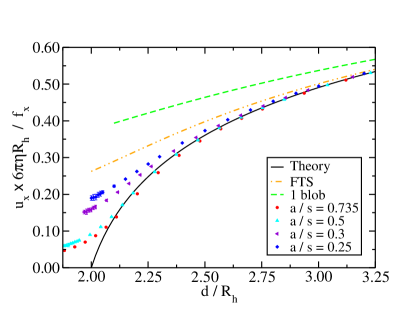
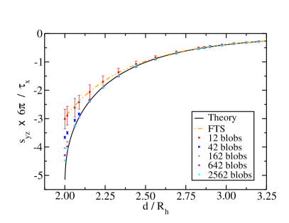
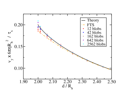
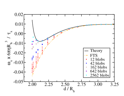
Figure 2: Hydrodynamic coupling between two identical spheres as a function of the center to center distance $d$. Twice the standard deviation as the two spheres are rotated relative to one another is shown as an error bar. Comparison is made to Stokesian dynamics without lubrication corrections, i.e., truncation at the FTS level, and to “exact” theory Brenner1961 ; SpheresStokes_JeffreyOnishi , see legend. The top left panel shows the average sphere velocity under the action of external unit forces $\boldsymbol{f}_{1}=-\boldsymbol{f}_{2}=\boldsymbol{f}$ directed along the line of collision, for a resolution of 162 blobs and for several values of $a/s$. The remaining three panels show non-trivial components of the pairwise mobility for a fixed $a/s=0.5$ and different resolutions (number of blobs per sphere, see legend). One sphere, located at $\left(\left(d{}^{2}-4R_{h}^{2}\right){}^{1/2},0,2R_{h}\right)$, is subject to an external torque of magnitude one around the $x$-axis. The response of the second sphere located at the origin is measured: the top right panel shows the stresslet $\boldsymbol{s}$ (i.e., the rotation-stresslet coupling), the bottom left panel shows the linear velocity (i.e., the rotation-translation coupling) $\boldsymbol{v}$, and the bottom right panel shows the angular velocity $\boldsymbol{\omega}$ (i.e., the rotation-rotation coupling) of the second sphere.

We explore the “lubrication” forces between spheres at very close distances in more detail in Fig. 3. In the left panel we show how the hydrodynamic force grows as the gap between the spheres decreases. The hydrodynamics of the low resolution models start to deviate from the theory for gaps $\sim R_{h}/2$ or smaller, while the highest resolution model (2562 blobs) shows a good agreement with the theory for gaps down to $0.1R_{h}$. The right panel of Fig. 3 shows the velocity error for one of the spheres with respect the exact theoretical result. For all models the error is below $10^{-3}$ until distances where the blobs forming the spherical shells start to overlap, which is the intuitive distance above which we expect the rigid multiblob to act as a good approximation to a sphere.

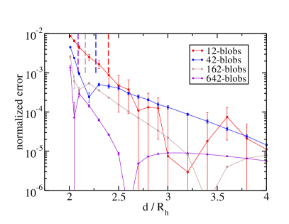
Figure 3: Lubrication forces on two identical spheres pulled toward each other with equal forces, for different resolutions (see legend). Twice the standard deviation as the two spheres are rotated relative to one another is shown as an error bar. (Left panel) Dimensionless normalized hydrodynamic resistance, i.e., the inverse of the hydrodynamic mobility shown in the top left panel in Fig. 2. (Right panel) Velocity error for one sphere with respect the exact theoretical result, normalized with the velocity at long distances ($f/6\pi\eta R_{h}$). The distance $d=2\left(R_{g}+a\right)$ at which blobs start to overlap is marked as a vertical line of the same color as the corresponding symbols.

In our second test, we measure the velocity of one sphere located at the origin when a second sphere, located at $(x,0,2R_{h})$, is subject to an external torque applied around the $x$-axis. Since the Brenner theory is only valid for spheres approaching along the line of collision we use the expansion of Jeffrey & Onishi accurate to order $\mathcal{O}\left(r^{-100}\right)$ SpheresStokes_JeffreyOnishi to compare with our mobility results; this expansion is also used in Stokesian Dynamics to compute near-field lubrication corrections for pairs of spheres and can be computed using the libStokes library of Ichiki libStokes . One can see on the lower panels of Fig. 2 that the low resolution model (12 blobs) is similar to a Stokesian dynamics model that includes monopole (forces) and dipole (torques and stresslet) terms but no lubrication corrections. As the resolution of the models is increased the results agree better with the theory, as expected. Note, however, that the lack of lubrication corrections in our models prevents a perfect agreement down to contact distances. In the top right panel of Fig. 2 we compare the stresslet computed on the particle at the origin. Again, we observe that the 12 blob model is similar in accuracy (aside from the presence of nonzero error bars, i.e., variance) to the Stokesian dynamic method without lubrication corrections, while higher resolutions methods agree better with the theory, as expected.

IV.3 Squirmer swimming speed

In this section we confirm the ability of our method to model an active sphere “squirmer” SquirmersFCM with a prescribed tangential surface slip on the surface. This slip $\breve{\boldsymbol{u}}_{i}=\breve{\boldsymbol{u}}\left(\boldsymbol{r}_{i}\right)$ takes the following form in spherical coordinates,

$$\breve{\boldsymbol{u}}_{r}=0,\quad\breve{\boldsymbol{u}}_{\phi}=0,\quad\breve{\boldsymbol{u}}_{\theta}=B_{1}\sin\theta$$

The active translational velocity of the squirmer is well-known to be the surface average of the surface slip SquirmerTheory_Stone ,

$$\boldsymbol{u}=-\langle\breve{\boldsymbol{u}}\rangle=\frac{2}{3}B_{1}\hat{\boldsymbol{z}}.$$

We have numerically computed the swimming speed of a squirmer in an unbounded domain for different resolutions and compared to the theory. We obtain that the relative error $\epsilon$ in the swimming speed is linear in $a/R_{g}$, which is expected. However, the error has a large prefactor, $\epsilon\approx 3.5\,a/R_{g}$, which is not small for the low-resolution models. Furthermore, observe that linear convergence with the size of the blobs implies only order one-half convergence in the number of blobs since the number of blobs required to cover the surface of the sphere grows quadratically with the sphere radius.

These findings confirm that the rigid multiblob models converge to the correct swimming speed but the accuracy is not very good. This is, in fact, not so surprising because we did not include any adjustments to account for the (potentially large) difference between the effective hydrodynamic radius $R_{h}$ and the geometric radius. That is, even though the effective no-slip surface has a radius $R_{h}>R_{g}$, we imposed the slip (in a locally-averaged way) at the surface of a sphere of radius $R_{g}$. We will investigate these issues and potential ways to improve the accuracy with which active slip is imposed in future work. Here we simply note that rigid multiblob models are well-suited to qualitative studies of suspensions of many active particles. If one wishes to accurately model one or a few active particles higher-order methods such as boundary integral methods are preferable.

IV.4 Suspension of spheres

In this section we study the convergence of the preconditioned Krylov solver for suspensions of many spheres. Our primary goal is to assess the effectiveness of our block-diagonal preconditioner for different packing densities (particle-particle distances) and numbers of particles. In the tests of this section we use spherical shells of 42 blobs subject to random forces, torques and slips. We form a finite cubic subset of a simple cubic lattice and place it in an unbounded fluid domain. We use right preconditioned GMRES without restarts, implemented using the PETSc PETSc library.

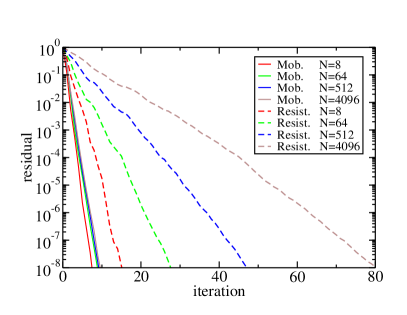
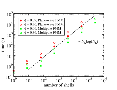
Figure 4: (Left panel) Convergence of preconditioned GMRES for the resistance and mobility problems for a finite subset of a cubic lattice of 42-blob spheres in an unbounded domain, for different number of particles, keeping the lattice spacing (closest distance between spheres) at $4R_{g}\sim 3.6R_{h}$ (corresponding to $\phi=0.09$). (Right panel) Wall-clock time to solve the mobility problem with a tolerance $10^{-8}$ versus the number of spherical shells for two volume fractions $\phi$, demonstrating the $\mathcal{O}(N_{b}\log(N_{b}))$ asymptotic complexity, where $N_{b}$ is the number of blobs. The matrix-vector product was computed with relative tolerance $0.5\cdot 10^{-9}$ using the FMM method developed in Ref. RPY_FMM . We compare the performance of a parallel multipole-based FMM3DLIB code OseenBlake_FMM with a more efficient but serial plane-wave FMM currently under development in the group of Leslie Greengard. Parallel runs used 8 cores and serial runs used a single core of an Intel Xeon 2.40GHz processor.

First, we test the robustness with increasing system size, keeping the particles well-separated at a distance $4R_{g}\approx 3.6R_{h}$, which corresponds to volume fraction $\phi\approx 0.09$. The left panel of Fig. 4 shows that the convergence is uniform and that the number of iterations to reduce the residual by a given factor depends very weakly on the number of spheres. This demonstrates the effectiveness of the block-diagonal preconditioner for the mobility problem. Next we investigate the robustness with respect to packing density. The right half of Table 1 shows the number of iterations to convergence for spheres arranged in a cubic simple lattice for several packing densities. When particles are far apart the solver converges fast because the hydrodynamic interactions between particles are weak and the preconditioner is designed to be an exact solver for a single body. As the spheres come closer together the preconditioner is not so effective and the Krylov solver needs to perform more iterations, as expected. However, even when the particles are relatively close the solver performs reasonably well. For example, when the spheres are at a distance of $2.55R_{g}\approx 2.3R_{h}$ ($\phi\approx 0.36$), the solver converges in 23 iterations. Of course, as the particles come closer and closer, and in particular, as the blobs on disjoint spheres begin to overlap, we expect to see an increasing ill-conditioning of the linear system (11) and an increasing number of iterations. However, the rigid multiblob method should not be used in this regime, since it does not accurately resolve lubrication forces at such short distances. In the right panel of Fig. 4 we show the wall-clock time to solve the mobility problem for different number of shells and volume fractions. Since the number of iterations is essentially independent of the system size we obtain a quasi-linear scaling by using the FMM to compute the product between the blob-blob mobility matrix and a vector.

However, for the resistance problem explained in Sec. II, the left panel of Fig. 4 shows that the number of iterations to attain convergence increase with the number of particles as $N^{1/3}$, i.e., with the linear extent of the system. This is somewhat better than the $O\left(N^{1/2}\right)$ iterations reported for Stokesian dynamics by Ichiki libStokes , but still much worse than the mobility problem.

We believe that this difference between resistance and mobility problems is physical rather than purely numerical. In particular, we expect that the same behavior will be observed in essentially any other iterative method, regardless of the specifics of the discretization of the problem (rigid multiblobs, boundary-integral methods, multipole expansions, regularized Stokeslets, etc.). To appreciate the difference between mobility and resistance problems, observe that it is possible to obtain a low accurate solution to the mobility problem by approximating each sphere by a single blob and then computing the matrix vector product $\boldsymbol{\mathcal{M}}\boldsymbol{f}=\boldsymbol{u}$ using an FMM. On the other hand, to solve the resistance problem the linear system $\boldsymbol{\mathcal{M}}\boldsymbol{f}=\boldsymbol{u}$ has to be solved, which must account for the collective nature of hydrodynamic interactions. The difference appears because there is an effective far-field two-body approximation for the mobility $\boldsymbol{\mathcal{N}}$ (equivalently for $\boldsymbol{\mathcal{M}}$) but not for the resistance matrix $\boldsymbol{\mathcal{N}}^{-1}$ (or $\boldsymbol{\mathcal{M}}^{-1}$), which is essentially a multibody problem RPY_Brinkman .

Mathematically, the difference appears because solving the saddle point problem (11) is similar to computing the motion for force- and torque-free particles IndefinitePreconditioning , even though forces and torques are applied on the particles. For force- and torque-free particles, the hydrodynamic fields and thus interactions with other particles decay faster than $1/r$. Therefore, the effective interactions that need to be captured by the iterative solver decay much faster for the mobility problem than for the resistance problem, making the former much easier. To confirm this intuition, we have studied (not shown) mixed resistance/mobility problems. When we fix the angular velocities but leave the linear velocities as free, we expect to see rapid convergence because the leading order interactions that the Krylov method needs to capture decay as $1/r^{3}$. Indeed, we observe numerically that in this case the solver converges almost as well as for the pure mobility problem. However, when we fix the linear velocities of the spheres but let them freely rotate, we find that the solver converges almost as bad as for the pure resistance problem.

V Results: Single Wall

In this section we study the accuracy of rigid multiblob models and the effectiveness of our block diagonal preconditioner for particle suspensions sedimented near a single no-slip boundary. This is an important and common occurrence in practice, especially in the field of active matter, since many active particles have metallic components and are not density-matched with the solvent, and thus sediment to the bottom substrate. Some of us studied the diffusive dynamics of nonspherical particles near a no-slip boundary using a rigid multiblob approach in Ref. BrownianMultiBlobs . However, in that prior work, we only studied a single body and therefore all of the mobility matrices were simply formed as dense matrices. Here we explore in more detail the accuracy of rigid multiblob models and also demonstrate how to scale rigid multiblob computations to suspensions of thousands of rigid bodies.

To compute the hydrodynamic interactions between blobs in the presence of a single wall we use a pairwise approximation to the blobs’ mobility which includes the effects of the wall in the Rotne-Prager tensor StokesianDynamics_Wall . In our implementation, we compute the product of the blob-blob mobility matrix $\boldsymbol{\mathcal{M}}$ with a vector using a direct $\mathcal{O}(N_{b}^{2})$ summation (here $N_{b}$ is the number of blobs) implemented on a GPU using PyCUDA PyCUDA in double precision; single precision can be used for lower accuracy requirements. This is an ideal problem for using GPUs as an accelerator since the computation is trivially parallelized on shared memory. Furthermore, the communication requirements between the CPU and GPU are minimal, since only the positions of the blobs need to be communicated . It is possible to implement a fast multipole method (FMM) for the RP(Y) tensor including wall corrections by using a system of images together with an FMM for unbounded domains RPY_FMM ; OseenBlake_FMM . However, it is important to note that the asymptotically-optimal FMMs on a CPU (even with multicore acceleration) will only be computationally more efficient than a direct sum on a GPU for more than about one hundred thousand blobs (in our testing on current hardware). Therefore, for many applications a simple GPU implementation is sufficient or even preferable over an asymptotically scalable implementation. Our PyCUDA codes are publicly available at https://github.com/stochasticHydroTools/RigidMultiblobsWall. Once a Rotne-Prager regularization of the construction of Gimbutas et al. OseenBlake_FMM is developed and combined with an FMM, the asymptotic cost will be reduced to $\mathcal{O}(N_{b}\log N_{b})$ and our computations can be extended to millions of blobs.

In section V.1 we study the accuracy of rigid multiblob models for modeling a sphere close to a boundary, and in Section V.2 we extend this study to a rigid cylinder (rod). In section V.3 we study the dynamics of a pair of active rods close to a no slip boundary. In section V.4 we study the performance of our iterative solver on a suspension of many rods, and demonstrate that the number of GMRES iterations is essentially independent of the number of particles just as for suspensions in an unbounded domain (see Section IV.4).

V.1 Sphere

In this section the mobility $\boldsymbol{\mu}\equiv\boldsymbol{\mathcal{N}}$ of a rigid multiblob sphere whose center is at a distance $H$ from a no-slip boundary is compared with some theoretical results available in the literature. We use the shell models of spheres described in Sec. IV, and show the mean and standard deviation of the computed mobility averaged over a large number of random orientations of the rigid multiblob relative to the boundary. To denote the specific component of the mobility matrix we use a subscript $tt$ for translational mobility, $rr$ for rotational mobility and $tr$ for translation-rotation coupling mobility, and we use a superscript $\perp$ or $\parallel$ to denote whether the direction of the force, torque, velocity or angular velocity is perpendicular or parallel to the wall.

The top left panel of Fig. 5 presents the translational mobility of the sphere perpendicular to the wall together with the exact theory obtained by Brenner Brenner1961 (see also Eq. (D2) in BrownianMultiBlobs for a simple but accurate approximation). We also compare to the complete expression for the Rotne-Prager-Blake tensor derived by Swan and Brady StokesianDynamics_Wall , including stresslet corrections, which corresponds to an FTS truncation (plus degenerate quadrupole corrections) of the multipole hierarchy. It is evident that a single-blob model of a sphere, just like the substantially more complicated FTS truncation, does not recover the strong drop in the mobility (i.e., lubrication) at small distances to the wall. Rigid multiblob models do substantially better than the FTS truncation even with only 12 blobs (icosahedral multiblob), and, as expected, the accuracy is improved with the addition of more blobs. As in the Sec.IV, the numerical mobility never goes exactly to zero since we do not add lubrication corrections, and we expect the rigid multiblob model to only work well when the blobs do not overlap the boundary itself. In fact, we recall here that the RP tensor we use here StokesianDynamics_Wall does not include near-field corrections when blobs overlap the wall, and therefore repulsive forces or other mechanisms should be used to ensure that the rigid multiblob is sufficiently far from the boundary. We empirically observe that the rotational invariance gets violated strongly if the gap to the wall is less than $2a/3$, which corresponds to 7% of the sphere radius for 12 blobs, and about 2% of the radius for the 642 blob model.

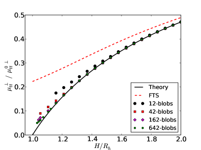
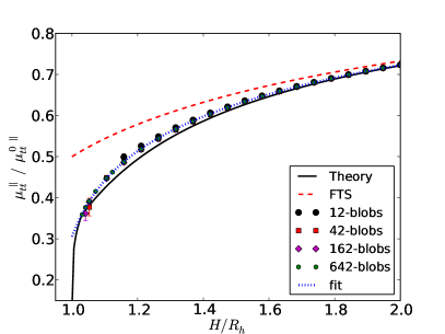
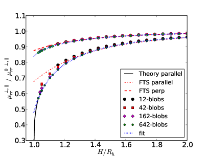
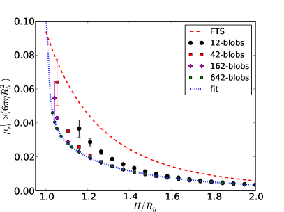
Figure 5: Selected components of the mobility $\boldsymbol{\mu}$ matrix for a sphere close to a wall, normalized by the corresponding bulk (unbounded domain) mobility $\boldsymbol{\mu}^{0}$ where possible. Comparison of the rigid multiblob results (symbols) is made to the best available theoretical results (solid black lines) and the FTS approximation used in Stokesian dynamics StokesianDynamics_Wall (dashed and dashed-dotted lines). Empirical fits listed in Appendix D are shown with a dotted line. (Top left) Translational mobility $\mu_{tt}^{\perp}$ for a force applied perpendicular to the wall. (Top right) Translational mobility $\mu_{tt}^{\parallel}$ for a force parallel to the wall. (Bottom left) Rotational mobility for a torque applied parallel ($\mu_{rr}^{\parallel}$, filled symbols) or perpendicular ($\mu_{rr}^{\perp}$, empty symbols) to the wall. (Bottom right) Rotation-translation coupling mobility $\mu_{tr}^{\parallel}$ for force or torque parallel to the wall.

In the remaining panels of Fig. 5 we investigate other components of the mobility. There are no closed-form expressions (even as infinite sums) for these components that are valid for all distances to the wall, so we use the best approximations available, see Appendix D in BrownianMultiBlobs for specific formulas. For the translational mobility parallel to the wall, shown in the top right panel of the figure, we use a result based on lubrication theory NearWallSphereMobility (see Eq. (D3) in BrownianMultiBlobs ) when the sphere is very close to the wall ($H<1.03R_{h}$), and an approximation to order $\mathcal{O}\left((H/R_{h})^{5}\right)$ for larger distances ConfinedSphere_Sedimented ; BrennerBook (see Eq. (D4) in BrownianMultiBlobs ). It is clear that the rigid multiblob matches the theory for large distances but that the approximate theory is not very accurate for $H\lesssim 1.5\,R_{h}$ since the rigid multiblob results are clearly converging to something slightly different. As for the perpendicular mobility, we see that the icosahedral model (12 blobs) is substantially more accurate than an FTS truncation.

Our results for the rotational mobilities, for torque applied either perpendicular or parallel to the wall, are shown in the bottom left panel of the figure and agree with the FTS results at large distances. We see slow but clear convergence of the rigid multiblob results for the translation-rotation coupling, shown in the bottom right panel of the figure. This component of the mobility is therefore most difficult to capture accurately, as is evident from the fact that the FTS truncation does pretty poorly in this case. Since neither the FTS truncation nor the asymptotic lubrication results NearWallSphereMobility are sufficiently accurate for comparison to experimental measurements, we have empirically fitted our highest-resolution results for the mobilities for which there are no exact theoretical expressions. We show the fits in Fig. 5 and give details about the fits in Appendix D for the benefit of other researchers.

V.2 Cylinder

In this section, we consider a cylinder (rod) of length $L=2.12$ and diameter $D=2R=0.325$ of aspect ratio $\alpha=L/D\approx 6.35$, mimicking the metallic rods studied in recent experiments TripleNanorods_Megan , for three different levels of resolution. The minimal resolution rigid multiblob has blobs placed in a row along the axis of the cylinder (a total of 14 blobs), while in the more resolved models, a hexagon (86 blobs) or a dodecagon (324 blobs) of blobs is placed along the circumference of the cylinder to better resolve it, as illustrated in Fig. 1. We study different components of the mobility matrix $\boldsymbol{\mu}\equiv\boldsymbol{\mathcal{N}}$; to specify the direction of the force, torque, velocity or angular velocity we use a subscript $\perp$ or $\parallel$ to denote whether the direction is perpendicular or parallel to the axes of the cylinder, respectively, and a superscript to denote whether the direction is perpendicular or parallel to the wall.

V.2.1 Bulk mobility

The first question that must be answered when constructing a rigid multiblob model of a given body is where to place the blobs and how to choose their hydrodynamic radius, to match the effective hydrodynamic response of the actual rigid body. Here we generalize the approach taken in Section IV.1 for spheres to a nonspherical body and show how to match the (passive) mobility of an actual rigid cylinder with a rigid multiblob model. Based on the results for spheres, for resolutions other than the minimally-resolved model we cover the surface (similarly for the ends of the cylinder) of a cylinder uniformly with spheres keeping the spacing between blobs both around the circumference and the length of the cylinder uniform and fixed at $a/s=0.5$.

Because there are no exact analytical results for the mobility of a cylinder even in an unbounded domain, we estimate the true mobility of the cylinder $\boldsymbol{\mu}^{0}$ in an unbounded domain numerically. Specifically, we place the blobs on the surface of a cylinder of length $L$ and radius $R$ (i.e., the true geometric surface of the actual rod we are modeling), and numerically compute the mobility for different resolutions. We then extrapolate to the limit $a\rightarrow 0$ using the two finest resolutions (86 and 324 blobs) based on our knowledge that the error is linear in $a$. For the translation-translation mobility we obtain $\left(\mu_{tt}^{0}\right)_{\parallel}\times 4\pi\eta L=3.404$ (compare to $3.295$ from slender-body theory SlenderBody_Cylinder ) and $\left(\mu_{tt}^{0}\right)_{\perp}\times 4\pi\eta L=2.606$ (compare to $2.619$ from slender-body theory SlenderBody_Cylinder ), while for the rotation-rotation mobility we get $\left(\mu_{rr}^{0}\right)_{\perp}\times\pi\eta L^{3}/3=1.212$ (compare to $1.211$ from slender-body theory IBM_Sphere ) and $\left(\mu_{rr}^{0}\right)_{\parallel}\times\pi\eta L^{3}/3=12.678$, see the last row in Table 2.

Our goal here is to match the bulk mobility $\boldsymbol{\mu}^{0}$ of our rigid multiblob models to that of a true cylinder as close as possible. To do this, for the surface-resolved models (86 and 324 blobs), we place the blobs on the surface of a cylinder of the same aspect ratio $\alpha=6.35$ but with the geometric radius $R_{g}$ of this cylinder allowed to be smaller than the geometric radius of the actual particle, while keeping the blob spacing $a/s=0.5$. We then numerically optimize the value of $R_{g}$ to minimize a measure of the error with respect to (extrapolated) mobility of a true cylinder, to obtain $R_{g}/R=0.90$ for the 86-blob model and $R_{g}/R=0.95$ for the 324-blob model. For the minimally-resolved model, we empirically tune both the geometric length (i.e., the distance between the centers of the two furthest blobs) to $L_{g}=0.914L$ and the blob radius to $a=1.103R$ while keeping the number of blobs fixed at $N_{b}=L/R+1=14$ as suggested by Bringley and Peskin IBM_Sphere . Table 2 shows the resulting infinite-domain mobilities for each resolution along with the relative error compared to the extrapolated values for infinite resolution. We see a relative error always less than $2.5\%$ even for the minimally-resolved model, except for rotation of the cylinder around its own axis; recall that the minimally-resolved model cannot support a torque around the axis of the cylinder.

Resolution	$\left(\mu_{tt}^{0}\right)_{\parallel}\times 4\pi\eta L$	$\left(\mu_{tt}^{0}\right)_{\perp}\times 4\pi\eta L$	$\left(\mu_{rr}^{0}\right)_{\perp}\times\pi\eta L^{3}/3$	$\left(\mu_{rr}^{0}\right)_{\parallel}\times\pi\eta L^{3}/3$
14 blobs	$3.422\,(-0.53\%)$	$2.612\,(-0.23\%)$	$1.216\,(-0.31\%)$	NA
86 blobs	$3.324\,(2.35\%)$	$2.541\,(2.48\%)$	$1.240\,(-2.34\%)$	$11.564\,(8.79\%)$
324 blobs	$3.360\,(1.29\%)$	$2.588\,(0.67\%)$	$1.225\,(-1.06\%)$	$12.274\,(3.19\%)$
$\infty$ (extrapolated)	$3.4040$	$2.6061$	$1.212$	$12.678$

Table 2: Nontrivial elements of the bulk mobility matrix for empirically-optimized rigid multiblob models of a cylinder of aspect ratio $6.35$, shown in the three left panels of Fig. 1. The value in the limit of infinite resolution is extrapolated numerically (see main text) and reported in the last row. The percentages in parenthesis correspond to the error relative to the infinite resolution estimates.

V.2.2 Mobility for a sedimented rod

Having determined the geometric parameters for the rigid multiblob models based on motion in an unbounded domain, we now study the accuracy of the three different resolutions for a cylinder close to a no-slip boundary. We assume that the cylinder is parallel to the wall with the centerline of the rod at a distance $H$ from the no-slip boundary.

Figure 6 compares the computed mobility coefficients to available theoretical and experimental results. As could be expected, the decrease in mobility when approaching the boundary is clearly underestimated with the minimally-resolved model. The left panel of the figure shows the translational mobilities. For $\mu_{\perp}^{\perp}$, the higher resolutions are in good agreement with the experimental measurements of Trahan and Hussey for a sedimenting rod with aspect ratio $\alpha=5.05$ CylinderWall_Experiments . Our numerical results also match well the theory of Jeffrey and Onishi InfiniteCylinderWall for an infinite cylinder when $H<2R$ . It is important to emphasize that our model is significantly more accurate than slender-body theory near boundaries; the slender-body theory results from SlenderCylinderWall_2 ; SlenderCylinderWall_1 ; SlenderBody_Cylinder (not shown here) are reasonably accurate only when $H/R>3.5$ for aspect ratios $\alpha>9$ CylinderWall_Experiments . The rotational mobilities of the rod are shown in the right panel of Fig. 6. For the rotational mobility $\mu_{\parallel}^{\parallel}$, all three resolutions are in good agreement with the theory of Jeffrey and Onishi InfiniteCylinderWall for an infinite cylinder. For $\mu_{\perp}^{\parallel}$ and $\mu_{\perp}^{\perp}$, the minimally-resolved model shows substantial errors near the wall, but the two higher resolution models agree with each other quite well over a broad range of distances.

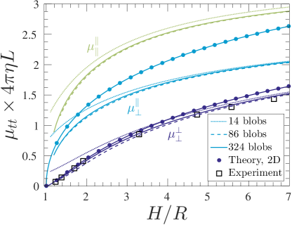
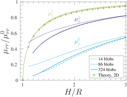
Figure 6: Mobility coefficients for a cylinder of aspect ratio $\alpha=L/\left(2R\right)=6.35$ when it is parallel to the wall, as a function of the height of the rod centerline $H/R$. The superscript of the mobility denotes the direction with respect to the wall, while the subscript denotes the direction with respect to the rod axis. (Left panel) Translational mobility coefficients $\boldsymbol{\mu}_{tt}$ normalized by $4\pi\eta L$ as in CylinderWall_Experiments . The curves with circles corresponds to the formulas from Jeffrey and Onishi for an infinite cylinder near a wall InfiniteCylinderWall . The black squares correspond to the experimental measurements of Trahan and Hussey for a rods with aspect ratio $\alpha=5.05$ CylinderWall_Experiments . (Right panel) Rotational mobility coefficients $\boldsymbol{\mu}_{rr}$ normalized by the corresponding bulk value. The curve with circles corresponds to an infinite cylinder near a wall InfiniteCylinderWall .

V.3 Active Rod Pair

In this section we apply the rigid multiblob method to a problem of recent experimental and theoretical interest: the dynamics of a pair of active “nanorods” that exhibit a “pusher” or extensile dipolar flow at large distances. Specifically, we compute the motion of a dimer of tripartite nanorods, as studied in recent experiments by Wykes et al. TripleNanorods_Megan . The rods have diameter of 0.325$\mu\mbox{m}$ and length of 2.12$\mu\mbox{m}$, and are in force and torque equilibrium (under the action of gravity and Van der Waals and electrostatic interaction forces with the boundary) at some distance from the wall that has not been measured in the experiments. The rods are constructed of three metal sections, in the arrangement gold-platinum-gold (Au-Pt-Au) and create a dipolar extensile (pusher) far-field flow. As such, they do not propel themselves in isolation but experiments show the formation of dimers of rods that actively rotate in a direction that is opposite of that predicted by recent simulations ActiveFilaments_Adhikari , which neglect the presence of the bottom wall. In agreement with the experiments, our simulations show the formation of a stable rod pair that touch each other tangentially and rotate (without exhibiting a significant translation) around an axis perpendicular to the wall in a direction consistent with the experimental measurements.

The exact details of the active flows near the surface of the rods have not been measured experimentally and are difficult to predict analytically because this requires resolving the thin slip boundary layer (of thickness related to the Debye length) around the rods, as well as the knowledge of a number of material constants that are not known accurately. To obtain a qualitative understanding of the dynamics of the rods we impose an apparent tangential surface slip velocity on the two gold sections, directed away from platinum center and having a magnitude of 20$\mu\mbox{m}/\mbox{s}$; no slip is imposed on the platinum section. Note that both gravity and the active slip pull the rods toward the wall, so we use an ad hoc repulsive force with the wall to balance the distance between the cylinder centerline and the wall at one cylinder diameter. Due to electrostatic interactions, a stacking of the two rods with the gold end of one rod aligned with the platinum center of the other is observed experimentally TripleNanorods_Megan ; here we study the flow around such a pair of aligned rods.

Figure 7: Active flow around a pair of extensile nanorods composed of three segments (shown with blue, green and red colors) sedimented on top of a no-slip boundary (the plane of the image) and viewed from above for the three different levels of resolution illustrated in Fig. 1: minimally resolved (left), marginally resolved (middle), and well resolved (right). The colored disks (red, blue or green) are projections of the blobs, with no-slip conditions on the green blobs and active slip of magnitude 20$\mu\mbox{m}/\mbox{s}$ on the blue and red blobs, directed away from the green segment. A cut through the flow field is shown in the lab frame as a vector field along with streamlines, with the magnitude of the velocity shown as a color scale plot.

In Fig. 7 we show the instantaneous flow around a dimer of active rods, as computed using the procedure described in Appendix B and seen from above, for three different resolutions: a minimally-resolved, a moderately-resolved and a well-resolved model. The imposition of the slip at the surface of the blobs becomes more and more accurate as the resolution is improved; however, we see a rather good match between the three flow fields even relatively close to the rods and wall. Our simulations, which correctly take into account the physical boundary conditions, estimate the angular frequency of rotation of the dimer to be approximately $0.64$Hz in the counter-clockwise direction, consistent with experimental observations TripleNanorods_Megan . The estimated angular velocities are $0.62,\,0.67$ and $0.63$Hz for each resolution respectively. We will study the dynamics of active nanorods near a no-slip surface in more detail in the future; in the next section we demonstrate that the calculations above can be scaled to suspensions of thousands of rods.

V.4 Suspension of rods near a boundary

In this section we test the efficiency of the preconditionner outlined in Section II.2 on a suspension of active rods sedimented near a wall. We have already seen that the block-diagonal preconditioner is able to account for the hydrodynamic interactions among the particles in a modest number of iterations for unbounded flow. Here we show that this continues to hold even when the wall strongly dominates the hydrodynamics, and investigate how important it is for the preconditioner to know about the presence of the boundary. Namely, recall that in the block-diagonal preconditioner the diagonal blocks of $\widetilde{\boldsymbol{\mathcal{M}}}$ correspond to the blob-blob mobility for an individual rod in the presence of the boundary. Since $\widetilde{\boldsymbol{\mathcal{M}}}$ depends on the configuration of each rod relative to the wall, unlike for an unbounded suspension, all diagonal blocks need to be factorized anew for each new configuration. However, it is also possible to use an approximate block diagonal preconditioner that assumes an unbounded suspension, i.e., neglects the presence of the boundary when computing a block-diagonal approximation of the blob-blob mobility. This seems like a strong approximation to be made for objects close to a no-slip wall; however, the investigations below will demonstrate that the Krylov solver can account not only for the rod-rod interactions, but also for the rod-wall interactions. This is an important finding because we recall that in the Green’s-function-free method described for confined suspensions in Section III, the boundary conditions are completely ignored in the preconditioner.

In these tests we discretize cylinders of aspect ratio $\alpha=L/D\approx 6.4$ either by placing $98$ blobs on the surface of a cylinder of geometric length $L_{g}=L$ and geometric radius $R_{g}=0.863R$, keeping $a/s=0.5$, or, by placing $21$ blobs of radius $a=1.02R$ uniformly spaced along a line segment of length $L$. For testing purposes, we generate random periodic packings of $N_{r}$ rectangles at a surface packing density $\phi_{a}$ using a molecular dynamics code Tetratic_Rectangles . We then use these hard-rectangle packings to generate a configuration of non-overlapping cylinders that are parallel to the wall and at a constant distance $H$ from the wall; we do not expect to see different results if some randomness is added to the heights and orientations of the cylinders relative to the wall, as long as their surfaces remain sufficiently far from the wall. In our tests we vary the centerline height $H$ from $H=0.75D$ to $H=2D$, the area fraction $\phi_{a}$ from $0.01$ to $0.6$, and the number of rods $N_{r}$ from $10$ to $10^{4}$; the number of blobs varies in the range from $N_{b}=200$ to about $N_{b}=10^{6}$. For our implementation and hardware (a Tesla K20 GPU) one GMRES iteration takes around $0.3s$ for $N_{b}=10^{4}$, $1s$ for $N_{b}\approx 2\cdot 10^{4}$, $20s$ for $N_{b}\approx 10^{5}$, and $220s$ for $N_{b}\approx 3\cdot 10^{5}$; we emphasize again that by using an FMM one can change the scaling from $O\left(N_{b}^{2}\right)$ to $O\left(N_{b}\log N_{b}\right)$ and thus substantially reduce the computational times for large $N_{b}$, see right panel in Fig. 4. To ensure a nontrivial right hand side of the linear system when testing the iterative solver, each blob is prescribed a random slip velocity and a random force, producing a random force and torque on each cylinder.

The left half of Table 3 shows the scaling of the number of GMRES iterations with the area fraction $\phi_{a}$ for a fixed number of rods $N_{r}=1000$, and compares the efficiency of the preconditioner using the full (wall-corrected) to that using the approximate (no wall contributions) block-diagonal preconditioner. We observe that the number of iterations increases slowly with the area fraction for both resolutions and reaches a maximum of 31 iterations for $\phi_{a}=0.6$ with the wall-corrected preconditioner. Therefore, as we already saw in Section IV.4, the performance of the preconditioner is not highly sensitive to near-field interactions. When using the approximate block-diagonal preconditioner without the wall corrections, the number of iterations is increased, as expected. However, this increase never exceeds $50\%$, which means that even a poor approximation of the mobility can be used in the preconditioner in practice. The right half of Table 3 shows the scaling of the preconditioner with the number of rods $N_{r}$ for a fixed area fraction $\phi_{a}=0.1$. The number of iterations rapidly saturates around 20 and becomes independent of the number of rods for both resolutions and heights. This confirms that the results obtained for a suspension of spheres in Section IV.4 apply to confined suspensions as well. Note that for the largest system sizes studied in the right half of Table 3 a linear-scaling FMM implementation would likely be substantially more efficient than the quadratic-scaling GPU implementation employed here.

$\phi_{a}$	Resolution	Wall-corrected	Unbounded
0.01	21	12	17
	98	16	28
0.1	21	19	23
	98	22	32
0.2	21	20	25
	98	23	34
0.4	21	25	29
	98	27	33
0.6	21	30	33
	98	31	43

$N_{r}$	Resolution	$H/D=0.75$		$H/D=2$
		iterations	time (s)	iterations	time (s)
10	21	7	0.15	7	0.15
	98	8	1.49	9	1.51
100	21	14	1.95	13	1.52
	98	19	18.9	18	35.6
1000	21	19	32.7	16	29.8
	98	22	620	20	559
5000	21	18	520	16	4,500
	98	23	10,200	22	12,400
10000	21	20	2,050	17	1,430
	98	23	39,400	21	36,300

Table 3: (Left) Number of GMRES iterations required to reduce the residual by a factor of $10^{8}$ for several surface packing fractions and two different resolutions (number of blobs per rod), for $H/D=0.75$ and $N_{r}=1000$ rods. The full block-diagonal preconditioner, which takes into account the wall corrections for each body, is compared to the approximate preconditioner, in which all wall corrections are neglected. (Right) Number of iterations and wall-clock time (using a direct GPU matrix-vector product on a Tesla K20 GPU) to solve the mobility problem with tolerance $10^{-8}$ using the wall-corrected preconditioner at $\phi_{a}=0.1$, for different number of rods and proximity of the rods to the wall.

VI Results: Confined Domains

In this section, we numerically explore the accuracy and efficiency of the rigid multiblob immersed boundary (IB) method described in Section III. This method is suited to fully confined (bounded) domains, and here we model suspensions of spheres in a periodic domain, a slit channel (i.e., two parallel walls), and a square (duct) channel. As discussed in more detail in Section III, for periodic suspensions it is possible to use FFT-based methods SpectralEwald_Stokes ; SD_SpectralEwald ; ForceCoupling_Fluctuations ; FluctuatingFCM_DC to obtain the product of the blob-blob mobility matrix with a vector. Future work should compare the method developed here with such approaches, especially for Brownian suspensions.

The effective hydrodynamic radius of an IB blob (also called a “marker” or “IB point” in the IB literature IBM_PeskinReview ) can be computed numerically by dragging a single blob with a constant applied force through a large periodic grid with spacing $h$ and applying the Hasimoto periodic correction ISIBM ; BrownianBlobs . When averaged over many positions of the marker relative to the underlying grid, for the six-point kernel New6ptKernel used here we obtain $a\approx 1.47\,h$. The geometry of the rigid multiblob models of a sphere used here is the same as in Sections IV and V. We also know from Section IV.2 that the spacing between the blobs should be around $s\approx 2a\approx 3h$, which is somewhat larger than the spacing $s\approx 2h$ used in RigidIBM , and leads to improved conditioning of the blob-blob mobility matrix. In fact, we observe that when distinct blobs overlap, the preconditioned GMRES solver described in Section III.3 shows significantly worse performance than when the blobs are not overlapping (or just touching). We therefore recommend using $s\gtrapprox 3h$ for rigid multiblob suspensions at zero Reynolds numbers.

Determining the exact spacing is somewhat of an art and is problem specific. In the IB approach developed here, the fast multipole method used in Section IV and the GPU matrix-vector product used in Section V are replaced by a geometric multigrid method, which works best for grid sizes that are powers of two. Once the exact spacing is determined, the effective hydrodynamic radius of the rigid multiblob can be determined numerically; we get very similar results for the IB method to those for an unbounded domain in Section IV.1, after setting $a=1.47\,h$. For confined suspensions, the ratio of the size of the particles to the domain size is typically fixed to some experimental value, and this constrains the choice of number of grid cells and spacing between the blobs. In all of the tests presented here, we have empirically optimized the appropriate value for the grid size and the spacing $s$ in the interval $2h$ to $3h$, and report the chosen values. As explained earlier, it is possible to use split IB kernels to gain more flexibility in choosing the grid sizes and blob spacing.

In Section VI.1, we investigate in more detail the loss of perfect translational and rotational invariance of the blob-blob mobility and the mobility of rigid multiblob spheres, and demonstrate that by using the improved six point kernel New6ptKernel our method is able to minimize the grid artifacts to a significant extent. Note, however, that there is an additional loss of rotational invariance for rigid multiblob models that comes from discretizing the bodies using blobs; this unphysical bias exists even in the absence of a fluid grid. In Section VI.2 we explore in more detail the accuracy for different resolutions for a periodic suspension of spheres by comparing to reference results from multipole-based methods. In Section VI.3 we compute the mobility of a sphere in a slit channel and compare to existing theories for a number of resolutions. In Section VI.4 we compute the effective quasi-two-dimensional diffusion coefficient of a boomerang colloid in a slit channel, and compare to recent experimental measurements BoomerangDiffusion ; AsymmetricBoomerangs ; angleBoomerangs . In Section VI.5 we optimize the convergence of the iterative linear solver for suspensions of many bodies, and demonstrate that the number of GMRES iterations is essentially independent of the number of particles, even in confined domains such as slit channels. Finally, we study the sedimentation velocities in a bidisperse suspension of spheres in Section VI.6, and compare to recent Stokesian Dynamics simulations BinarySuspension_SD ; SD_SpectralEwald . In Appendix C we study flow around permeable rigid bodies.

VI.1 Translational invariance

As explained in detail in Section III, for sufficiently large domains the blob-blob mobility computed by the IB method has the approximate form (22). Deviations from this formula arise because of the imperfect translational and rotational invariance due to grid artifacts. The two functions $f(r)$ and $g(r)$ are expected to be similar to those appearing in the RPY tensor (9). We obtain the actual form of the functions $f(r)$ and $g(r)$ empirically by fitting numerical data for the parallel and perpendicular mobilities of a pair of blobs placed in a large periodic domain, see RigidIBM for more details. The results are shown in the left panel of Fig. 8, and are compared to the RPY tensor for spheres of radius $a=1.47h$. We have empirically fitted the numerical results for $f(r)$ and $g(r)$ with a fit that has the proper asymptotic behavior at large and short distances, see Appendix A in RigidIBM for more details; this fit is used in the preconditioner as an analytical approximation of the diagonal blocks of the blob-blob mobility matrix. We see that the differences between the fits and the RPY tensor are rather small, and also confirm the improved translational invariance of the six-point kernel New6ptKernel as evidenced in the small scatter of the points around the fits. This confirms our expectation that the rigid multiblob IB method will behave similarly to an RPY-based method in terms of accuracy.

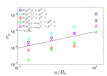
Figure 8: Translational and rotational invariance of the rigid multiblob IB method. (Left panel) Empirical values of the blob-blob mobility functions $f(r)$ and $g(r)$ appearing in (22), normalized by $8\pi\eta r$ so that they asymptote to unity. An empirical fit through the data is compared to the RPY tensor for blob radius $a=1.47h$. Note that the scatter around the fit for $r\gtrsim 5a$ is dominated by periodic artifacts due to the finite size of the grid. (Right panel) Standard deviations of the diagonal (translation-translation, rotation-rotation) and cross-coupling (rotation-translation) components of the mobility matrix for spheres discretized with 12, 42, 162 or 642 markers shells (i.e., for decreasing $a/R_{h}$). Also shown is the typical magnitude of the off-diagonal components of the translation-translation and rotation-rotation mobility matrices, which should be zero for a perfect sphere.

In the right panel of Fig. 8 we investigate the translational and rotational invariance of rigid multiblob models of spheres as a function of the resolution. We randomly move and rotate a sphere relative to the underlying grid and compute the elements of the mobility matrix. The mean of these elements defines an effective translational and rotational radius consistent with the results presented in Section IV.1 (not shown). In the figure we show the normalized standard deviation of the elements of the mobility matrix as a function of the resolution (number of blobs). As expected, the normalized standard deviation decreases linearly with the size of the blobs $a$ (equivalently, the inverse of the square root of $N_{b}$), and is below $10^{-4}$ for all mobility elements even for the 12-blob (icosahedral) model MultiblobSprings .

VI.2 Periodic Suspension of Spheres

In this section we apply our rigid multiblob method to a benchmark resistance problem in a periodic suspension of 108 spheres moving with random linear and angular velocities. This benchmark was developed by Anthony Ladd, who supplied us with a random and a face-centered cubic (FCC) configuration of spheres, at a low density of $\phi=0.05$, as well as a high density of $\phi=0.45$. He also supplied to us the results for the resulting forces and torques obtained using the HYDROMULTIPOLE code HYDROMULTIPOLE . Note that pairwise lubrication corrections have been included in the multipole expansion method used for these calculations HYDROMULTIPOLE ; HydroMultipole_Ladd ; HydroMultipole_Ladd_Lubrication ; to our knowledge no method has accounted for three-body lubrication corrections.

The rigid multiblob models used in this study have been chosen to give a blob spacing close to $s\approx 2a\approx 3h$, while ensuring that the number of grid cells is integer given the specified unit cell length in the benchmark configurations, and to have a specified effective hydrodynamic radius $R_{h}\approx 1$ for five different resolutions: a single blob per sphere (similar to a truncation with only one monopole per sphere), 12 blobs (geometric radius $R_{g}=0.7896$, grid spacing $h=0.2778$), 42 blobs ($R_{g}=0.8899$, $h=0.1667$), 162 blobs ($R_{g}=0.9502$, $h=0.08929$) and 642 blobs ($R_{g}=0.9766$, $h=0.0463$) per sphere. The results for the $x$ component of the computed forces on the spheres are illustrated in Fig. 9; similar results are observed for other components.

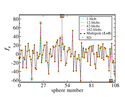
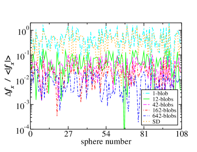
Figure 9: Results from the rigid multiblob method applied to Ladd’s benchmark resistance problem (with specified random velocities) for a periodic suspension of 108 spheres. (Left panel) The $x$-component of the force on each sphere in a random suspension at a low volume fraction $\phi=0.05$. For comparison, we show the results of Stokesian dynamics (SD) libStokes and the HYDROMULTIPOLE code HYDROMULTIPOLE with $L=8$ moments retained. Two particles that happen to be at a distance closer than $2.02$ radii from each other are marked by a black box and a blue circle, and develop unresolved strong lubrication forces between them. (Right panel) The normalized error $\left|f_{x}-f_{x}^{(\text{ref})}\right|/\langle\left|f_{x}^{(\text{ref})}\right|\rangle$ in the $x$-component of the force for an FCC lattice at the high volume fraction $\phi=0.45$. The HYDROMULTIPOLE code with $L=8$ moments is used as a high-accuracy reference calculation.

In the left panel of Fig. 9, we focus on the low density suspension ($\phi=0.05$) and compare the forces computed by the rigid multigrid method with those computed using $L=8$ multipole moments, as well as the results of the Stokesian dynamics (SD) code of Ichiki libStokes (which roughly corresponds to $L=2$ moments). The overall agreement is quite good, but notice that even with $162$ blobs per sphere we do not resolve the lubrication force between particles numbered 48 and 103, marked in the figure, since this pair of particles have a gap of only $0.024$ radii between them. This is not surprising given that we do not include pairwise lubrication corrections in our method; such corrections are included in the reference results we are comparing to so they produce accurate forces for all particles. In the rigid multiblob method, we resolve the near field interactions more and more accurately as we increase the number of blobs per sphere, but we cannot accurately resolve the hydrodynamic interactions between pairs of particles with overlapping blobs (see Fig. 2).

At the high packing fraction $\phi=0.45$ there are many pairs of nearly touching particles in a typical random suspension of hard spheres in the absence of (electrostatic) repulsive forces, and there is no hope that the rigid multiblob method can accurately compute the interparticle forces . Therefore, at this density we focus on an FCC lattice configuration, and compare to the multipole-based code with $L=8$ moments. Here the closest particle distance is $2.36$ radii and our method is able to resolve the forces relatively well, especially with more than 12 blobs per sphere, see the right panel in Fig. 9. This is perhaps not surprising; however, the more important point we wish to make is that the SD results are now not significantly more accurate than the results obtained from using only a single blob per sphere. The addition of stresslets and pairwise lubrication does not appear to help much in resolving the many-body far field hydrodynamic multiple scattering in this lattice configuration. Using an icosahedral rigid multiblob already provides an order of magnitude improvement in the typical error over an FTS truncation, and provides an error comparable to keeping $L=3$ moments in the HYDROMULTIPOLE method (not shown), which is also the minimum number of moments necessary to keep to capture all long-ranged hydrodynamic interactions, as well as to model active sphere suspensions BoundaryIntegralGalerkin ; IrreducibleActiveFlows_PRL .

VI.3 Sphere in a slit channel

In this section we compute the parallel and perpendicular translational mobilities of a sphere in a slit channel of thickness $19.2R_{h}$ as a function of the height $H$ of the sphere center above one of the walls. This problem is of relevance to a number of experiments involving spherical colloids confined between two glass microscope slips, and has also been used as a benchmark problem for boundary integral calculations in BoundaryIntegral_Wall . Since the immersed boundary method used here cannot be used for infinite domains, we take a domain of dimensions $(76.8,\,19.2,\,76.8)R_{h}$ and apply no-slip conditions on the $y$ boundaries and periodic conditions in the other two directions.

There are no manageable theoretical results accurate for all distances from the wall and all channel dimensions StokesianDynamics_Slit . For the parallel component of the mobility, Faxen obtained exact series expansions for the mobility at the half and quarter channel locations, which we use to benchmark our calculations, neglecting the corrections coming from the use of periodic boundary conditions in the directions parallel to the walls. For other positions of the sphere we employ the Modified Coherent Superposition Assumption (MCSA) approximation given in Eq. (9) in Ref. MobilitySlitChannel , with the mobility relative to a single wall given by the same theoretical lines shown in Fig. 5. The rigid multiblob models used in this study have been chosen to give a blob spacing close to $s\approx 2a\approx 3h$, while ensuring that the number of grid cells is integer given the target channel width relative to the effective hydrodynamic radius of the sphere $R_{h}$ for all of the resolutions studied: a single blob as a minimal model of the sphere BrownianBlobs (grid size $128\times 28\times 128$), 12 blobs (grid size $256\times 64\times 256$, geometric radius $R_{g}=2.503h$, giving spacing $s/h=2.63$), and 42 blobs ($512\times 128\times 512$ grid, $R_{g}=6.047h$, $s/h=3.30$).

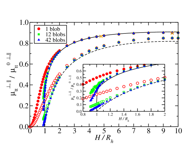
Figure 10: Translational mobility of a sphere in a slit channel of width $19.2R_{h}$ relative to the bulk, for several resolutions of the rigid multiblobs (see legend), for forces/motion parallel (filled symbols) and perpendicular (empty symbols) to the wall. The numerical results are in good agreement with the exact results of Faxen for distances $H=L/4$ and $H=L/2$ (orange crosses). The inset shows that close to the wall the results for the $12$ and $42$ blob shells are in reasonable agreement with the approximate MCSA theory (lines).

We have already confirmed that our results are in agreement with Faxen’s theory in the (extrapolated) limit of an infinitely long channel in our prior work RigidIBM . Here we examine the mobility as the sphere moves through the channel, and in particular, as it comes close to the wall. The results of our calculations are shown in Fig. 10, and are in good agreement with the approximate MCSA theory for the parallel mobility. Note that the MCSA theory is approximate even far from the wall, as seen from the fact that our results do not match it for the perpendicular mobility even at the center of the channel. The boundary condition handling described in Appendix D of RigidIBM ensures that for a single blob the mobility vanishes at the boundary, i.e., for $H=0$, rather than for $H=R_{h}$ as for a true sphere. The more resolved models, however, do show a sharp drop in mobility when the sphere nearly touches the wall. The inset shows that the lubrication interactions are not resolved very close to the wall, just as we observed for a single wall in Section V.1. Nevertheless, we note that unlike the Rotne-Prager-Blake mobility tensor computed by Swan and Brady StokesianDynamics_Wall and used in Section V.1, the mobility computed by the grid-based Stokes solver is physically realistic even when the blobs overlap the wall. This has two important implications. First, the rigid multiblob IB method does not run into singularities for $H_{\text{min}}<H<R_{h}$, where $H_{\text{min}}$ is the distance at which the center of some blob first leaves the physical domain. This is particularly beneficial in Brownian simulations, where stochastic motion can push the sphere to slightly overlap the wall BrownianBlobs ; BrownianMultiBlobs . Furthermore, the immersed boundary results in the inset of Fig. 10 are substantially more rotationally-invariant as the sphere approaches the wall than the corresponding results in the top two panels of Fig. 5; the error bars in the mobility due to discretization artifacts are very small for the immersed boundary method even for $H<R_{h}$.

VI.4 Boomerang in a slit channel

In this section we study the diffusion of a boomerang colloidal particle in a narrow slit channel, as recently studied experimentally and theoretically BoomerangDiffusion ; AsymmetricBoomerangs ; angleBoomerangs . The boomerangs are confined to essentially remain in the plane parallel to the wall by the tight confinement, and thus perform quasi two-dimensional diffusion. We previously studied the diffusion of such a boomerang colloid sedimented against a single no-slip boundary in BrownianMultiBlobs , using a strong gravitational force to keep the boomerang in quasi two dimensions. However, the colloids in the actual experiments are almost neutrally buoyant and a slit channel is used to confine them to two dimensions. Here we use our rigid multiblob IB method to determine the effective two dimensional diffusion coefficients of a single boomerang in slit confinement.

As discussed in detail in BrownianMultiBlobs , it is, in principle, necessary to perform long Brownian simulations to determine the long-time diffusion tensor $\boldsymbol{D}$ of nonspherical particles. However, if the mean square displacement (MSD) is linear in time, the long and short-time time diffusion coefficients are equal and can be obtained from the Stokes-Einstein relation

$$\boldsymbol{D}=k_{B}T\left\langle\boldsymbol{\mathcal{N}}\right\rangle=k_{B}T\,\bar{\boldsymbol{\mu}},$$ (29)

where $\bar{\boldsymbol{\mu}}$ is the average mobility over configurations following the Gibbs-Boltzmann (GB) distribution. Therefore, the diffusion coefficient can be computed by generating samples from the GB distribution of boomerang configurations, and then solving a mobility problem for each configuration and averaging over the samples. For quasi two-dimensional diffusion the MSD can be made nearly linear by a careful choice of the tracking point BrownianMultiBlobs ; BoomerangDiffusion ; AsymmetricBoomerangs , which is the point whose translation is measured and around which torques are expressed bernal1980transport . Chakrabarty et al. BoomerangDiffusion have shown that for particles diffusing in two dimensions, the optimal choice of tracking point is the center of hydrodynamics stress (CoH), the location of which can be computed from the bulk mobility tensor BrownianMultiBlobs .

To compare with the experimental results of Chakrabarty et al. we compute the diffusion coefficient of a single boomerang colloidal particle between two walls. In the experiments BoomerangDiffusion , colloidal particles with boomerang shape diffuse in a channel of width $\sim 2\mu m$. The boomerang particles, produced by photolithography, have two arms of length $2.1\mu m$, thickness $0.51\mu m$ and width $0.55\mu m$ forming a right angle. In our computations, we use no-slip boundary conditions on the walls of the channel and periodic boundary conditions in the directions parallel to them. We construct two rigid multiblob models of such boomerangs (see BrownianMultiBlobs for geometric details): a minimally resolved model with 15 blobs (grid size $128\times 9\times 128$, blob spacing $s/h=1.36$) that is essentially a bent version of the cylinder model shown in the left-most panel of Fig. 1, and a moderately resolved model with 120 blobs (grid size $256\times 18\times 256$ and blob spacing $s/h=2.22$), shown in the right-most panel of Fig. 1.

We assume a hard-core potential between each of the blobs and the walls, and average the mobility over 100 samples generated from the Gibbs-Boltzmann distribution using an accept-reject Monte Carlo procedure BrownianMultiBlobs . In the experiments, there is likely an additional electrostatic repulsion from the wall; we have checked that adding a short-ranged Yukawa-type repulsion with the walls does not change our results significantly . Following BoomerangDiffusion , we report the diffusion coefficients computed using (29) in the continuous body frame (CoB) BoomerangDiffusion attached to the colloidal particle, such that the axis $X_{1}$ goes along the line that bisect the boomerang angles and the axis $X_{2}$ is orthogonal to $X_{1}$ (see Fig. 1 in BoomerangDiffusion ). The diffusion coefficient for the boomerang particle are given in Table 4. We see that the computed location of the CoH is in good agreement with experimental estimates. However, both translational and the rotational in-plane diffusion coefficients computed in the simulations are twice larger than those measured experimentally, for both resolutions.

	Experiments	ratio = (Experiment / Simulation)
		15 blobs	120 blobs
$d$	$1.16\;(\mu m)$	1.06	1.06
$D_{11}$	$0.049\;(\mu m^{2}/s)$	0.55	0.47
$D_{22}$	$0.058\;(\mu m^{2}/s)$	0.50	0.46
$D_{\theta}$	$0.044\;(\mbox{rad}^{2}/s)$	0.46	0.46

Table 4: Comparison of experimentally-measured diffusion coefficients for a boomerang particle in a slit channel to numerical estimates obtained from the rigid multiblob IB method. The tracking point is chosen to be the CoH, which is a point on the boomerang bisector line at a distance $d$ (first row) from the crossing point of the two boomerang arms. We report the translational diffusion coefficients $D_{11}$ and $D_{22}$ in the Continuous Body Frame (CBF) of reference as in Ref. BoomerangDiffusion , averaged over 100 samples from the Gibbs-Boltzmann distribution of particle configurations, for two different resolutions.

To investigate this large mismatch between simulations and experiments, we explore further the difference between the right angle boomerangs used in the two distinct experiments BoomerangDiffusion (arms of length $2.1\mu m$ and width $0.55\mu m$) and angleBoomerangs (arms of length $2.33\mu m$ and width $0.7\mu m$), both for a reported channel width of $2\mu m$. The boomerangs in angleBoomerangs are reported to be about 10% larger than those used in BoomerangDiffusion ; however, the reported diffusion coefficients are reported to be about 25% larger. This is inconsistent with a purely hydrodynamic model, since the larger particles should have smaller bulk diffusion coefficients and are more confined. Therefore, the larger particles must have a translational diffusion coefficient that is more than $1.1$ times smaller for translation, and more than $1.1^{3}\approx 1.33$ times smaller for rotation, if particle size is the only difference between the two experiments. Indeed, in our simulations the translational diffusion coefficient is about $1.25$ times smaller for the larger particles, and the rotational one is $1.57$ times smaller. This suggest that there are some unreported experimental effects that are not taken into account in the simulations, such as a potentially non-uniform channel thickness or polydispersity in the particles. More careful future investigations are required to understand the origin of the difference between simulations and experiments reported in Table 4.

VI.5 GMRES convergence

In this section we investigate the performance of the preconditioner described in Sec. III.3 and determine an optimal value for $N_{s}^{(1)}$ and $N_{s}^{(2)}$, the number of iterations in the first and second approximate Stokes solves in the preconditioner. As a Krylov solver, here we use the restarted right-preconditioned GMRES method, but we have also observed good performance with the short-term recurrence BiCGStab method, which typically requires a few more iterations than GMRES but has smaller memory requirements. It is important to emphasize that the exact number of iterations depends strongly on the geometry of the rigid multiblobs, notably, the spacing between the blobs. The performance depends even more strongly on the efficacy of the geometric multigrid preconditioner for the Poisson equation, which in the implementation used here is strongly degraded for grids that have a nearly prime number of cells in each dimension, and for grids of large aspect ratios (even if all directions are powers of two). Our focus here is on investigating the trends in the number of GMRES iterations with the various parameters in the preconditioner and the system size.

The computational cost of the solver is dominated by the application of the full preconditioner, whose complexity depends on nontrivial ways on its different steps and on the parameters of the simulations. However, in most cases the cost is dominated by the multigrid cycles for the Poisson equation, and each application of the projection preconditioner for the Stokes equation (28) involves $d+1=4$ scalar V cycles. Here we use preconditioned Richardson iteration as an iterative solver for the (unconstrained) Stokes equations . Therefore, the total number of scalar multigrid cycles per GMRES iteration is $4(N_{s}^{(1)}+N_{s}^{(2)})$ and we can use $N_{s}^{(1)}+N_{s}^{(2)}$ as a proxy for the computational cost. It should be noted, however, that this is only an approximation and in practice it may be better to allow a small increase on the total number of Stokes preconditioner applications if it reduces significantly the number of outer GMRES iterations.

We study the solver convergence for a random bidisperse suspensions of hard spheres with aspect ratio $R_{h,1}/R_{h,2}=1/2$ at different concentrations and system sizes and geometries. The parameters of the rigid multiblob models are identical to those reported in Section VI.3. We investigate a suspension at a moderate volume fraction $\phi=0.15$ ($\phi_{1}=\phi_{2}=0.075$ for the two components), as well as a suspension at a high volume fraction $\phi=0.45$ ($\phi_{1}=\phi_{2}=0.225$). We investigate three different types of boundary conditions, a periodic suspension in a cubic domain, a suspension in a slit channel with periodic boundaries in the directions parallel to the wall, and a square channel with periodic boundaries in the direction of the channel axis. The configurations of hard spheres were generated using a Monte Carlo algorithm with hard core exclusion radius equal to the effective hydrodynamic radius of the spheres.

In the left panel of Fig. 11 we show the relative residual versus the number of iterations of the outer solver for different values of $N_{s}^{(1)}$ and $N_{s}^{(2)}$. Because of all of the approximations in the analytical blob-blob mobility matrix, the convergence does not improve with increasing $N_{s}^{(1,2)}$ beyond some point. Therefore, it is not necessary to perform nearly exact Stokes solves (e.g., complete FFTs in periodic domains) inside the preconditioner; a few (spectrally equivalent) cycles of multigrid are sufficient. In the inset in the right panel of Fig. 11 we show that the total number of applications of the Stokes preconditioner $N_{s}=\left(N_{s}^{(1)}+N_{s}^{(2)}\right)N_{\text{iter}}$ is a reasonable proxy for the computational time, where $N_{\text{iter}}$ is the number of GMRES iterations .

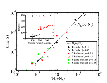
Figure 11: (Left panel) Convergence of GMRES with restart frequency of 60 iterations for a bidisperse suspension of spheres in a cubic periodic domain (filled symbols, grid size $128^{3}$, $N_{s}=1014+127=1141$ spheres), and in a slit channel of dimensions $4L\times L\times 4L$ (open symbols, grid size $256\times 64\times 256$, $N_{s}=6083+760=6843$ spheres). All spheres are subject to random forces, torques and slips. (Left panel) Normalized residual versus number of iterations of the outer solver for different number of iterations in the first ($N_{s}^{(1)}$) and second ($N_{s}^{(2)}$) Stokes subsolves inside the preconditioner. For comparison, we also solve the Stokes subproblems to high accuracy using an inner iteration of GMRES, marked $N_{s}^{(1)}=N_{s}^{(2)}\gg 1$ in the legend. (Right panel) Total computing time to solve the mobility problem as a function of the number of spheres $N_{s}=N_{1}+N_{2}$ using an implementation based on the IBAMR library and eight cores of an Intel Xeon (E5-2665, 2.4GHz) processor. The inset shows the time to solve the linear system versus the total number of Stokes preconditioner applications $(N_{s}^{(1)}+N_{s}^{(2)})\,N_{\text{iter}}$.

Table 5 shows the number of GMRES iterations required to reduce the residual by a factor of $10^{8}$ for a variety of system sizes, keeping $N_{s}^{(1)}=2$ and $N_{s}^{(2)}=1$. As seen in the table, the convergence for periodic domains, just as for the methods based on Green’s functions studied in Sections IV.4 and V.4, is independent on the system size and only depends weakly on the packing density. The largest system has a grid of $512^{3}$ cells and almost $3.4$ million blobs on $2.2\cdot 10^{5}$ spherical shells packed to a rather high density $\phi=0.45$, yet the GMRES iteration converges after only 44 iterations. For confined systems the solver requires more iterations, as expected because the boundary conditions are not taken into account in either the Stokes solver preconditioner nor the block-diagonal mobility approximation. At first sight, it may appear that the number of iterations grows with the system size for non-periodic domains. This increase, however, comes not because of the increase in system size but rather because the aspect ratio of the domain grows and the multigrid algorithm used in our implementation becomes less effective. This can be confirmed by noting that the number of iterations grows very weakly with system size if we keep the domain aspect ratio fixed; for a square channel and $\phi=0.45$ we require $58$ iterations for a grid with $128\times 64\times 64$ cells, 60 iterations for $256\times 128\times 128$ cells, and 65 iterations for $512\times 256\times 256$ cells (compared to 119 for $512\times 64\times 64$ cells). This demonstrates that our preconditioner robustly handles large system sizes even in the presence of physical boundaries. We believe the performance of the solver for high-aspect ratio domains can be greatly improved with a new multigrid implementation capable of dealing with highly non-cubic domains at the coarsest levels of the multigrid hierarchy. The right panel of Fig. 11 shows the total computing time as a function of system size and demonstrates the near linear scaling of the method at fixed computing power, at least for cubic periodic domains, for which the multigrid implementation used in the IBAMR library is nearly optimal.

$\phi$	Periodic				Slit channel				Square channel
	cells	$N_{1}$	$N_{2}$	$N_{G}$	cells	$N_{1}$	$N_{2}$	$N_{G}$	cells	$N_{1}$	$N_{2}$	$N_{G}$
0.15	$128\times 128\times 128$	1014	127	28	$128\times 64\times 128$	507	63	34	$128\times 64\times 64$	283	32	37
	$256\times 256\times 256$	8111	1014	29	$256\times 64\times 256$	$2028$	$253$	42	$256\times 64\times 64$	507	63	47
	$512\times 512\times 512$	64885	8111	29	$512\times 64\times 512$	$8111$	$1014$	63	$512\times 64\times 64$	1014	127	65
0.45	$128\times 128\times 128$	3041	380	42	$128\times 64\times 128$	1521	190	52	$128\times 64\times 64$	760	95	58
	$256\times 256\times 256$	24332	3041	43	$256\times 64\times 256$	6083	760	62	$256\times 64\times 64$	1521	190	76
	$512\times 512\times 512$	194656	24332	44	$512\times 64\times 512$	24332	3041	96	$512\times 64\times 64$	3041	380	119

Table 5: GMRES convergence results for a bidisperse suspension in periodic and confined domains. A random configuration of $N_{1}$ hard spheres of radius $R_{h}=1$ (12 blobs) and $N_{2}$ hard spheres of radius $R_{h}=2$ (42 blobs) is generated, and random forces, torques and slips are applied on all of the particles. We report the number of GMRES iterations $N_{G}$ needed to reduce the residual by a factor $10^{8}$ for the mobility problem for a variety of system sizes and boundary conditions.

VI.6 Sedimentation velocity in a binary sphere suspension

In our last test we use our rigid multiblob IB method to compute the mean and variance of the instantaneous sedimentation velocity in a random binary suspension of hard spheres, as done using Stokesian Dynamics (SD) by Wang and Brady BinarySuspension_SD ; SD_SpectralEwald . The binary suspension has two components, $\alpha=1$ and $\alpha=2$, with equal volume fractions $\phi_{1}=\phi_{2}=\phi/2$ and size ratio $R_{2}/R_{1}=2$. The two types of particles are assumed to be much denser than the solvent and to have the same density, so that the ratio of the gravitational forces is set to $F_{2}/F_{1}=8$. Here we average the sedimentation velocity statistics over an ensemble of sphere packings that are sampled from the equilibrium distribution in the absence of gravity. To generate configurations of spheres, we use the Lubachevsky-Stillinger packing algorithm Event_Driven_HE to create an initial packing of spheres, and then use equilibrium event-driven hard sphere MD to equilibrate the packings. We then apply gravitational forces on all spheres and solve the mobility problem to compute the instantaneous sedimentation velocities $U_{s,\alpha}$ for each species. As described in more detail in RigidIBM , the total gravitational force on the spheres must be balanced by an equal and opposite uniform force density in the fluid because of the use of periodic boundary conditions.

The rigid multiblob models used in this study have either 12 blobs ($R_{g}=0.6643$, $R_{h}\approx 1$, $s/h=2.052$) for the smaller species and 42 blobs for the larger species ($R_{g}=1.7714$, $R_{h}\approx 2$, $s/h=2.843$), or, for improved resolution, 42 blobs for the smaller species ($R_{g}=0.8692$, $R_{h}\approx 1$, $s/h=2.553$) and $162$ blobs for the larger species ($R_{g}=1.8935$, $R_{h}\approx 2$, $s/h=2.808$). To correct for finite system size effects, for each volume fraction $\phi$ we run simulations for three grid resolutions, specifically, we use grids of size $64^{3}$, $128^{3}$, and $256^{3}$ cells for the smaller resolution ($12-42$ blobs per sphere), and $128^{3}$, $256^{3}$, $512^{3}$ for the higher resolution ($42-162$ blobs). The average sedimentation velocity was extrapolated to the infinite system size limit by assuming that the finite-size corrections scale as $1/N^{-1/3}$, where $N$ is the total number of particles, instead of assuming a specific analytical form for the corrections BinarySuspension_SD ; SedimentationMonodisperse_Ladd . The largest example in our simulations is for $\phi=0.5$ with a $512^{3}$ grid, for $N_{1}=51,200$ and $N_{2}=6,400$ spheres, corresponding to a total of about 10 million Lagrangian (i.e., blob/body) degrees of freedom (DoFs), and about half a billion Eulerian (i.e., fluid) DoFs.

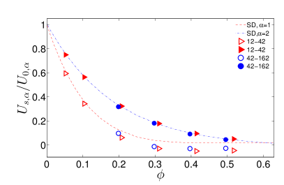
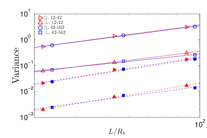
Figure 12: Instantaneous sedimentation rates of the two species, $\alpha=1$ (empty symbols) and $\alpha=2$ (filled symbols), in a binary suspension of hard spheres, for two different resolutions (see legend). (Left panel) Average vertical sedimentation velocity normalized by $U_{0,\alpha}=F_{\alpha}/(6\pi\eta R_{\alpha})$ as a function of the total volume fraction $\phi$. The data from recent Stokesian dynamics simulations BinarySuspension_SD is shown as lines. (Right panel) Normalized variance $\Delta U_{\alpha}^{2}=\langle\delta U_{s,\alpha}^{2}\rangle/U_{0,\alpha}^{2}$ of the sedimentation velocity parallel and perpendicular to gravity for $\phi\approx 0.2$. Linear fits to the data are shown as dashed lines.

The left panel of Fig. 12 compares our results for the mean sedimentation velocity of the different species with results obtained using traditional (i.e., non-accelerated) SD without pairwise lubrication corrections BinarySuspension_SD . It is well known that a standard FTS truncation is not particularly accurate for sedimentation because of the importance of a nontrivial mean quadrupole SedimentationMonodisperse_SD , therefore, the SD simulations include a mean-field estimate of the quadrupole contribution, see Eq. (2.29) in SD_Suspensions . Such a correction is not included in the accelerated SD method developed in SD_SpectralEwald , and this leads to a strong over-estimation of the sedimentation velocity at larger densities and even a reversal of the trend toward increasing sedimentation rate SD_SpectralEwald . Our results show a consistently decreasing sedimentation rate with increasing density, and are in good agreement between the two resolutions, except that the agreement is only qualitative at the higher densities for the smaller spheres (thus indicating a lack of convergence in our numerical results). Our results are consistent with the SD results for the larger particles over the range of densities studied here. However, for the smaller particles we find a smaller sedimentation rate and even a negative rate, which arises due the strong backflow created around the larger particles. As discussed in Section VI.2, lubrication forces can be very important at densities as large as $\phi=0.5$, although they are often assumed to play little role in sedimentation due to lack of relative motion among the particles, and are therefore not included in the SD simulations. Neverthess, it may be that lubrication forces play a role for dense binary suspensions due to the relative motion of the small spheres around the large spheres. We therefore believe that the binary sedimentation problem should be revisited by more accurate methods or experiments.

The right panel of Fig. 12 shows the normalized variance of the instantaneous sedimentation velocities for the two species at $\phi=0.2$ as a function of system size. Consistent with theory and simulation for random suspensions of monodisperse suspensions SedimentationMonodisperse_Ladd , we find that the variance grows linearly with system size, consistently between the two resolutions. This unphysical growth has been the subject of a long-standing controversy in the literature, which cannot be resolved by our static (i.e., instantaneous) computations. Namely, it has been noted that the structure of the suspension changes during sedimentation SedimentationMonodisperse_Ladd2 , although not enough to suppress the variance growth in existing Lattice Boltzmann (LB) simulations SedimentationMonodisperse_Ladd . More recent LB studies have suggested that boundaries, polydispersity and stratification all play roles in the sedimentation of a realistic suspension SedimentationMonodisperse_Ladd3 .

VII Conclusions

In this paper we described a numerical method for simulating non-Brownian Stokesian suspensions of passive and active rigid particles of essentially arbitrary shape in either unconfined, partially confined, and fully confined geometries. Following a number of prior works, we discretized rigid bodies using a collection of minimally-resolved spherical blobs to move as a rigid body. A key contribution of our work was the development of preconditioned iterative solvers for the potentially large linear system of equations for the unknown Lagrange multipliers $\boldsymbol{\lambda}$ and rigid-body motions $\boldsymbol{U}$. We demonstrated that an effective and scalable approach is to solve the saddle-point problem for both $\boldsymbol{\lambda}$ and $\boldsymbol{U}$ using a block-diagonal preconditioner that ignores hydrodynamic interactions of distinct bodies, or even interactions between the bodies and the boundary.

The hydrodynamic interactions between the blobs are captured using the Rotne-Prager-Yamakawa (RPY) tensor tailored to the specific geometry (boundary conditions). For unbounded domains, we used a fast multipole method to compute the product of the blob-blob mobility $\boldsymbol{\mathcal{M}}$ and a force vector. For a single no-slip boundary, we used a GPU to directly sum the Rotne-Prager-Blake tensor over all pairs of blobs; FMM methods for half-space Stokes flow have recently been developed OseenBlake_FMM and could be used to scale these computations to millions of blobs. We showed empirically that the number of GMRES iterations required to solve for $\boldsymbol{\lambda}$ and $\boldsymbol{U}$ is bounded independent of the number of bodies, and grows only weakly with increasing packing density. This paves the way for the development of linear-scaling methods for solving the mobility problem in moderately dense suspensions of hundreds of thousands of particles. At the same time, we find that solving the resistance problem is substantially more difficult since the number of iterations grows approximately linearly with the linear dimensions of the system.

For more complex boundary conditions such as fully confined domains, there is no simple analytical approximation to the RPY tensor RPY_Periodic_Shear . While it is possible to construct fast methods for computing the product $\boldsymbol{\mathcal{M}}\boldsymbol{\lambda}$ in specific geometries, e.g., using Ewald summation for periodic domains RigidMultiblobs_Swan , this requires knowing the Green’s function analytically, and more importantly, requires a new method and code for each specific combination of boundary conditions. As an alternative, in this work we developed a rigid multiblob method for periodic suspensions or suspensions confined in slit and square channels that uses a grid-based Stokes solver to compute the action of the (regularized) Green’s function “on the fly” BrownianBlobs ; BrownianDynamics_OrderN ; BD_IBM_Graham . Specifically, we extended a recently-developed rigid-body immersed boundary method RigidIBM to suspensions of freely-moving passive or active rigid particles at zero Reynolds number. We demonstrate that GMRES applied to the coupled fluid plus rigid body equations converges in a bounded number of iterations independent of the system size, with a weak growth of the number of iterations with the packing density, and a moderate growth with increased confinement. Unlike in methods based on Green’s functions, each Krylov iteration in our approach only requires a few cycles of a geometric multigrid solver for the Poisson equation, and an application of the block-diagonal preconditioner for the blob-blob mobility.

We used our methods to compute the mobility of a cylinder near a no-slip boundary and found good agreement with experimental measurements. We also demonstrated that a pair of active pusher tripartite nanorods sedimented near a boundary form dimers that rotate in a direction consistent with recent experimental measurements TripleNanorods_Megan . Our numerical results for the effective planar diffusion coefficient of a boomerang colloid confined to a narrow slit channel were not in agreement with recent experimental measurements BoomerangDiffusion ; angleBoomerangs by a factor of two. In the future we will carry out more careful and systematic quantitative comparisons between simulations and experiments for confined passive and active colloids.

It is worthwhile to point out some specific differences between our approach and existing methods. We focus in this comparison on methods based on Green’s functions. For confined domain, our Green’s-function-free method described in Section III is quite different from most existing methods. The equations (10) appear, perhaps in somewhat modified form, in a number of works HYDROPRO ; HYDROPRO_Globular ; RotationalBD_Torre ; HYDROLIB ; SphereConglomerate ; RigidBody_SD ; Multiblob_RPY_Rotation . The key distinguishing feature of our work is the use of iterative methods as a way to scale these computations to suspensions of thousands of bodies. While preconditioned iterative solvers have been used in the recent work of Swan and Wang RigidMultiblobs_Swan , we believe the preconditioned saddle-point approach developed here is notably superior both in efficiency and simplicity.

The rigid multiblob approach is quite similar to the method of regularized Stokeslets developed by Cortez et al. RegularizedStokeslets ; RegularizedStokeslets_2D ; RegularizedStokeslets_Walls ; RegularizedStokeslets_Periodic . This method is usually presented as a regularized first-kind boundary integral formulation RegularizedStokeslets for solving (35). The method has been made more accurate by using higher-order quadratures RigidRegularizedStokeslets ; RegularizedStokesletsPhoretic , and has very recently been generalized to second-kind formulations that account for active slip RegularizedStokesletsPhoretic . However, these works do not consider preconditioners and existing regularized Stokeslet methods do not scale well to many-body suspensions. We note that a first-kind formulation preconditioned by a block-diagonal preconditioner as we do in this work is spectrally equivalent to a second-kind formulation for well-separated bodies . In RegularizedStokesletsPhoretic double layer terms (i.e., second-kind boundary integrals) are included to account for the active slip. As we argued in Appendix A.1, this is not necessary if one is not interested in surface tractions, and therefore we prefer our simpler regularized first-kind formulation. Another key difference between our approach and the method of regularized Stokeslets is that the mobility used in regularized Stokeslets methods is different from the RPY tensor; most importantly, it is not symmetric. Notably, Cortez et al. apply the regularization on the forces (sources) but not also on the velocities (targets), which approximately corresponds to omitting $\left(\boldsymbol{I}+a^{2}/6\,\boldsymbol{\nabla}_{\boldsymbol{r}}^{2}\right)$ in (7). Using a non-symmetric blob-blob mobility is not physical, for example, incorporating thermal fluctuations becomes impossible since this requires the square root of the mobility.

Our work is very closely related to that of Swan, Brady et al. StokesianDynamics_Wall . The following are key differences. First, we use only the RPY form of the mobility matrix, that is, we only have a force (monopole) degree of freedom at each blob, as done in more recent work by Swan and Wang RigidMultiblobs_Swan . This can be seen as a direct but regularized discretization of (35), where the unknown is the surface “traction”. By contrast, Swan et al. use Stokesian Dynamics (SD) to represent the blobs as “spheres”, more precisely, to associate with each blob a force, torque and stresslet (FTS) ; more multipoles have been included in other works based on multipole expansions SphereConglomerate ; ActiveFilaments_Adhikari ; ConstrainedFCMChains . This makes the number of degrees of freedom (DoF) per blob at least $3+3+5=11$ in three dimensions, instead of just $3$ as in our formulation. In recent work Multiblob_RPY_Rotation , rotational degrees of freedom (angular velocity and constraint torques) have been added to the blobs without including stresslets (i.e., an FT truncation), which doubles the number of DOFs per blob relative to the approach we follow (6 DOFs instead of 3). Our investigations have shown this to lead to insufficient improvement in accuracy to justify the doubling of the number of DOFs. For active suspensions, in the formulation of ActiveFilaments_Adhikari ; BoundaryIntegralGalerkin ; Galerkin_Wall_Spheres , active slip is imposed on the surface of the beads composing the rigid body, i.e., each bead is active individually. By contrast, our blobs do not really have a well-defined surface, and in our formulation active slip is imposed on the surface of the body and not on blobs individually, consistent with a discretization of (35). Our approach only requires a way to compute the (action of the) RPY blob-blob mobility matrix, and is therefore much simpler to use in practice and adopt to different boundary conditions. As we explained in Section III, the RPY tensor can be approximated using grid-based solvers quite straightforwardly using immersed boundary methods, but going to higher orders requires additional differentiability (smoothness) ForceCoupling_Stokes than afforded by simple immersed boundary methods.

Another key difference between the rigid multiblob method and traditional Stokesian dynamics is that we do not include lubrication (near-field) corrections in addition to the far-field RPY mobility. If it is necessary to resolve near-field interactions between particles, for example, to study the rheology of concentrated suspensions, one can increase the resolution by using more blobs per rigid body. For sufficiently dense suspensions, very close contacts become numerous and in practice lubrication forces need to included as a correction to the FTS expansion. We choose, however, not to include uncontrolled pairwise lubrication approximations for several reasons. First, we believe that it is important to control the approximations so that accuracy can be confirmed by comparing different levels of resolution. Second, it is difficult to generalize pairwise lubrication corrections to dense suspensions of rigid particles of arbitrary shape.

We carefully studied the accuracy of the rigid multiblob approach on a variety of standard problems for spherical particles. We demonstrated that, once the effective hydrodynamic radius of the rigid multiblobs is matched to the target sphere radius, even a 12-blob (icosahedral) model of a sphere MultiblobSprings provides a substantial improvement over the widely-used force-torque-stresslet (FTS) truncation of the multipole hierarchy, especially near boundaries. However, we note that the rigid multiblob models are not rotationally invariant and this leads to notable discretization artifacts as blobs on distinct bodies begin to overlap. Furthermore, our method does not include pairwise lubrication corrections for nearby pairs of spheres (for reasons discussed in the body of the paper), and can therefore only accurately resolve the hydrodynamic interactions between objects if the blobs on the two bodies do not overlap each other. It remains as a grand challenge for future work to construct a scalable method that applies to particles of complex shape with complex boundary conditions and resolves lubrication interactions among nearly touching particles with controllable accuracy.

There are a number of possible extensions of the computational method described here. An important direction of work is to compute a tractable formulation of the RPY-Blake tensor for a single no-slip boundary that ensures an SPD mobility matrix even when blobs overlap the wall, which is important for the inclusion of thermal fluctuations (Brownian motion). While a general SPD formulation of RPY in confined domains has been developed in RPY_Periodic_Shear , that formulation does not apply a regularization when the blobs overlap the wall . Such a regularization is important physically, in particular, we believe it is crucial that the velocity of a blob go to zero smoothly as its position approaches the boundary. This prevents unphysical motion of blobs along the no-slip boundary, or even worse, blobs leaving the domain. Observe that the alternative formulation of the blob-blob mobility (21), together with the modification near no-slip boundaries first proposed by Yeo and Maxey ForceCoupling_Channel and generalized to other boundary conditions in Appendix D in RigidIBM , is SPD for all configurations and vanishes as a blob approaches a boundary. If the integral in (21) can be performed analytically for some choice of the kernel $\delta_{a}$, this would give a simple formula for a Rotne-Prager-Yamakawa-Blake tensor that can be used in practical simulations. Another approach to constructing a regularization is to use the simple image construction proposed recently by Gimbutas et al. OseenBlake_FMM and combine with the free-space RPY tensor.

The rigid multiblob formulation can be seen as a low-order regularized quadrature rule for the first-kind integral equation (35). It is natural to consider using higher-order quadrature rules. This has been done in the context of the method of regularized Stokeslets in RigidRegularizedStokeslets ; RegularizedStokesletsPhoretic , and has been done in the context of immersed boundary methods in IBFE . Specifically, Griffith and Luo have proposed an alternative IB approach that models the deformations and stresses of immersed elastic body using a finite element (FE) representation IBFE . In their IB/FE approach, the degrees of freedom associated with $\boldsymbol{\lambda}$ are represented in a finite-element basis set, and the interaction between the fluid grid and body mesh is handled by placing IB markers at the numerical quadrature points of the FE mesh. When such an approach is generalized to rigid bodies, it simply amounts to filtering the mobility operator (26),

$$\boldsymbol{\mathcal{M}}_{FE}=\boldsymbol{\Psi}\left(\boldsymbol{\mathcal{J}}\boldsymbol{\mathcal{L}}^{-1}\boldsymbol{\mathcal{S}}\right)\boldsymbol{\Psi}^{T}=\boldsymbol{\Psi}\boldsymbol{\mathcal{M}}\boldsymbol{\Psi}^{T},$$

where $\boldsymbol{\Psi}$ is a matrix that contains quadrature weights as well as geometric information about the FE mesh. Future work should explore whether this approach provides a significant improvement in accuracy or efficiency over the simple rigid multiblob approach presented here, and to compare this to the methods described in RigidRegularizedStokeslets ; RegularizedStokesletsPhoretic .

In the method used here, we used a regular (staggered) grid and therefore no-slip boundary conditions can only be imposed on the boundaries of a rectangular prism. Domains of complex shapes, such as (patterned) microfluidic channels, can be handled in two ways. The first way is to construct the boundaries out of rigidly fixed blobs BD_IBM_Graham . While this is flexible and straightforward, it requires solving a combined mobility-resistance problem that our investigations suggest cannot be solved scalably using existing methodologies. An alternative and promising approach is to use an FEM method to solve the Stokes equations on a boundary-fitted unstructured tetrahedral grid SELM_FEM , and combine this with the rigid-body immersed boundary ideas presented here. Even if a rectangular grid is appropriate, our regular-grid method requires very large grids for very low densities or inhomogeneous suspensions, such as, for example, a suspension of particles sedimented near a bottom wall in a slit channel where the top wall needs to be taken into account as well. A substantial challenge for future work is to develop a stable discretization of the steady Stokes equations on an adaptively-refined (e.g., block structured) staggered grid; this has been accomplished for unsteady flow IBAMR but the steady Stokes equations pose several notable challenges.

We believe that a number of the preconditioning ideas developed in this work can also be applied to other related methods, such as methods based on boundary integral formulations. Some of these methods can provide a notable improvement in accuracy over the low-accuracy rigid multiblob method, and with a suitable preconditioner they can potentially be scaled to suspensions of tens of thousands of particles. For certain simple confined geometries, such as periodic boundaries or semi-infinite slit channels, it is possible to develop fast methods for applying the RPY and related tensors based on FMM or FFT methods. This may be preferable to the immersed boundary approach followed here, which requires a dense grid of spacing smaller than the hydrodynamic radius of the blobs $a$. By contrast, the spectral Ewald method SpectralEwald_Stokes completely decouples the spacing of the FFT grid from $a$, while controlling the accuracy. We believe that is important for the community working on Stokes suspensions to develop benchmark problems and compare different methods in terms of both accuracy and efficiency, to identify which methods are most appropriate under which conditions and accuracy requirements.

To account for thermal fluctuations (Brownian motion), one adds a fluctuating component $\left(k_{B}T\eta\right)^{\frac{1}{2}}\left(\boldsymbol{\mathcal{Z}}\left(\boldsymbol{r},t\right)+\boldsymbol{\mathcal{Z}}^{T}\left(\boldsymbol{r},t\right)\right)$ to the fluid stress $\boldsymbol{\sigma}$ in (31) BrownianBlobs ; ForceCoupling_Fluctuations ; SELM ; FluctuatingFCM_DC in the spirit of fluctuating hydrodynamics VACF_Langevin ; LangevinDynamics_Theory ; LLNS_Staggered , where $\boldsymbol{\mathcal{Z}}\left(\boldsymbol{r},t\right)$ denotes a white-noise random Gaussian tensor field with uncorrelated components. This adds a fluctuating component to the rigid-body velocity and leads to the overdamped Langevin equation

$$\left[\begin{array}[]{c}\boldsymbol{u}\\ \boldsymbol{\omega}\end{array}\right]=\left[\begin{array}[]{c}d\boldsymbol{q}/dt\\ d\boldsymbol{\theta}/dt\end{array}\right]=\boldsymbol{\mathcal{N}}\left[\begin{array}[]{c}\boldsymbol{f}\\ \boldsymbol{\tau}\end{array}\right]-\breve{\boldsymbol{\mathcal{N}}}\breve{\boldsymbol{u}}+\left(2k_{B}T\,\boldsymbol{\mathcal{N}}\right)^{\frac{1}{2}}\diamond\boldsymbol{\mathcal{W}}\left(t\right).$$ (30)

where $\boldsymbol{\mathcal{W}}\left(t\right)$ denotes a collection of independent white-noise scalar processes and $\diamond$ denotes a suitable (kinetic) stochastic product KineticStochasticIntegral_Ottinger ; BrownianMultiBlobs . In this work we did not consider the generation of the fluctuating component of the rigid-body motion $\left(2k_{B}T\,\boldsymbol{\mathcal{N}}\right)^{\frac{1}{2}}\boldsymbol{W}$, where $\boldsymbol{W}$ is a collection of standard normal variates. This is an important missing component for suspensions in an unbounded or half-space domain. For the immersed boundary method described in Section III, computing the random motion of rigid multiblobs is straightforward and can be accomplished at essentially no additional cost by simply including the stochastic stress on the right-hand side in the fluid equations. The difficulty, which we will address in future work, is to develop a temporal integration scheme for (30) that correctly accounts for the stochastic drift terms without incurring significant additional costs compared to non-Brownian suspensions BrownianBlobs ; FluctuatingFCM_DC ; BrownianMultiBlobs .

Appendix

Appendix A Continuum Formulation

The basic problem we consider is the motion of a number of rigid bodies suspended in a Stokesian fluid. For simplicity, consider a single body $\Omega$ rotating with angular velocity $\boldsymbol{\omega}$ around a tracking point (origin) that is translating with linear velocity $\boldsymbol{u}$, under the combined influence of an external force $\boldsymbol{f}$ and torque $\boldsymbol{\tau}$; the generalization to many bodies is straightforward. Without loss of generality let us assume that the fixed (lab) and body coordinate frames are identical at the point in time under consideration. Outside the body we have the steady Stokes equations for the fluid velocity $\boldsymbol{v}\left(\boldsymbol{r}\right)$ and the pressure $\pi\left(\boldsymbol{r}\right)$,

$$-\boldsymbol{\nabla}\cdot\boldsymbol{\sigma} =\boldsymbol{\nabla}\pi-\eta\boldsymbol{\nabla}^{2}\boldsymbol{v}=0$$ (31)

$$\boldsymbol{\nabla}\cdot\boldsymbol{v} =0,$$

along with some suitable boundary conditions at infinity or the boundary of a domain $\mathcal{D}\supset\Omega$. The no slip boundary condition on the surface of the body is

$$\boldsymbol{v}\left(\boldsymbol{q}\right)=\boldsymbol{u}+\boldsymbol{\omega}\times\boldsymbol{q}+\breve{\boldsymbol{u}}\left(\boldsymbol{q}\right)\mbox{ for all }\boldsymbol{q}\in\partial\Omega,$$ (32)

where $\breve{\boldsymbol{u}}$ is a specified apparent slip velocity due to active boundary layers on the surface of the rigid body. Here $\boldsymbol{u}$ and $\boldsymbol{\omega}$ are Lagrange multipliers for the force and torque balance conditions,

$$\int_{\partial\Omega}\boldsymbol{\lambda}\left(\boldsymbol{q}\right)d\boldsymbol{q}=\boldsymbol{f}\quad\mbox{and}\quad\int_{\partial\Omega}\left[\boldsymbol{q}\times\boldsymbol{\lambda}\left(\boldsymbol{q}\right)\right]d\boldsymbol{q}=\boldsymbol{\tau},$$ (33)

where $\boldsymbol{\lambda}\left(\boldsymbol{q}\right)$ is the normal component of the stress on the outside of the surface of the body, i.e., the traction

$$\boldsymbol{\lambda}\left(\boldsymbol{q}\right)=\boldsymbol{\sigma}\cdot\boldsymbol{n}\left(\boldsymbol{q}\right),$$

where $\boldsymbol{n}$ is the surface normal and the fluid stress is

$$\boldsymbol{\sigma}=-\pi\boldsymbol{I}+\eta\left(\boldsymbol{\nabla}\boldsymbol{v}+\boldsymbol{\nabla}^{T}\boldsymbol{v}\right).$$ (34)

The solution of the above system of equations is, by linearity, an affine mapping of the form (1).

A.1 Boundary integral re-formulation

Observe that in the Stokes regime, the details of what happens inside the body do not actually matter for the motion of the body and its hydrodynamic interactions with other bodies or boundaries. For instance, a fluid-filled “bacterium” with a rigid membrane and a solid particle of the same shape will move identically for the same surface slip and total force and torque. Similarly, to an outside observer, a bacterium covered with a layer of cilia on the outside will be indistinguishable from a bacterium that also has a layer of cilia on the inside of its membrane. Therefore, it is possible to extend the fluid equation (31) to the whole domain and pretend that there is fluid inside the body moving with a velocity that is continuous across the boundary of the body. For a strictly rigid body motion on the surface, the fluid inside will move as a rigid body and thus be free of strain RegularizedStokeslets . If there is slip on the surface, when we extend the flow inside we are assuming that the velocity is continuous at the boundary so that the same slip is present on the inside of the body surface. This will drive internal active flows inside the body in addition to the external active flow outside. Once we extend the fluid equation everywhere we can write down an equivalent first-kind boundary integral equation for Stokes flow BoundaryIntegral_Pozrikidis ; RegularizedStokeslets

$$\boldsymbol{v}\left(\boldsymbol{q}\right)=\boldsymbol{u}+\boldsymbol{\omega}\times\boldsymbol{q}+\breve{\boldsymbol{u}}\left(\boldsymbol{q}\right)=\eta^{-1}\int_{\partial\Omega}\boldsymbol{\mathbb{G}}\left(\boldsymbol{q},\boldsymbol{q}^{\prime}\right)\tilde{\boldsymbol{\lambda}}\left(\boldsymbol{q}^{\prime}\right)d\boldsymbol{q}^{\prime}\mbox{ for all }\boldsymbol{q}\in\partial\Omega,$$ (35)

which along with the force and torque balance condition (33) defines a linear system of equations to be solved for the single-layer potential $\tilde{\boldsymbol{\lambda}}\left(\boldsymbol{q}\right)$ and the velocities $\boldsymbol{u}$ and $\omega$. Here $\boldsymbol{\mathbb{G}}\left(\boldsymbol{q},\boldsymbol{q}^{\prime}\right)$ is the Green’s function for steady Stokes flow with unit viscosity and with the specified boundary conditions on the domain boundary $\partial\mathcal{D}$.

In this work we will require that the total volume of fluid is preserved by the slip, i.e., there is no source or sink for the flow inside the particle (as would be the case for swelling bodies),

$$\int_{\partial\Omega}\breve{\boldsymbol{u}}\left(\boldsymbol{q}\right)\cdot\boldsymbol{n}\left(\boldsymbol{q}\right)d\boldsymbol{q}=0,$$ (36)

which is always true for tangential slip. This condition is required to be able to extend the flow inside the body and still keep it incompressible everywhere in the domain. This condition is related to a known issue with first-kind boundary integral formulations having a nontrivial null space, or, equivalently, the single layer operator having an incomplete range BoundaryIntegral_Pozrikidis . Removing the restriction (36) requires switching to a second-kind or a mixed first-second kind integral equation RegularizedStokesletsPhoretic ; BoundaryIntegralGalerkin .

The single-layer potential $\tilde{\boldsymbol{\lambda}}\equiv\boldsymbol{\lambda}=\boldsymbol{\sigma}\cdot\boldsymbol{n}$ if there is no slip, i.e., if $\breve{\boldsymbol{u}}=0$, which is a property that relies closely on the fact that the specified velocity on the surface of the body is a rigid-body velocity, see the book of Pozrikidis BoundaryIntegral_Pozrikidis for details but also RegularizedStokeslets for a simple and relevant derivation using a regularized (non-singular) Green’s function. If there is slip, then $\boldsymbol{\lambda}$ does not have a direct physical interpretation as a surface traction, rather, it is the jump in the stress when going across the body surface from the “interior” flow to the “exterior” flow. If one wants to determine the actual traction in the presence of nontrivial slip a second kind integral formulation ought to be used, which includes an additional term on the right hand side of (35) involving $\breve{\boldsymbol{u}}$ BoundaryIntegral_Pozrikidis ; StokesSecondKind_Shelley ; BoundaryIntegralGalerkin . The fact that the same force and torque balance condition (33) applies even though $\boldsymbol{\lambda}$ is not the physical traction follows from the fact that the fictitious fluid inside the body is not accelerating; equivalently, one observes that a double-layer density does not contribute to the total force and torque on the body since it is a dipole rather than a monopole density. As discussed at length by Cortez et al. RegularizedStokeslets , both the method of regularized Stokeslets and the rigid multiblob method presented here can be seen as a particularly straightforward technique for solving a suitably regularized version of (35) RegularizedStokesletsPhoretic ; RigidRegularizedStokeslets .

Appendix B Computing flow fields

Observe that, unlike the immersed boundary method, the Green’s-function-based rigid multiblob method described in Section II does not compute the actual flow (velocity and pressure) around the bodies. Rendering flow fields is useful in a number of applications for visualizing the flow around passive and active rigid bodies. There are a number of different ways to define a flow field around a multiblob, here we follow the following procedure that reuses existing code and produces smooth non-singular flow fields everywhere, including inside the blobs. The input to the calculation are the constraint forces $\boldsymbol{\lambda}$, and the output is a fluid velocity $\boldsymbol{v}\left(\boldsymbol{r}\right)$ evaluated at an arbitrary position in the domain.

The basic idea is to estimate the velocity that a freely-moving tracer blob of a given size $a^{\prime}\ll a$ would have, where $a^{\prime}$ is a desired resolution scale for the flow that could be chosen to match the size of actual tracer particles used in an experiment. We replace each of the $N_{b}$ blobs with $N_{b}^{\prime}$ smaller blobs of radius $a^{\prime}$, i.e., we treat each blob $i$ as a sphere of radius $a$ and discretize it using smaller blobs. We divide the constraint force on blob $i$ uniformly (this is consistent with the approximation used to construct the RPY tensor RPY_Shear_Wall ) among the small blobs, $\boldsymbol{\lambda}_{j}^{\prime}=\boldsymbol{\lambda}_{i}/N_{b}^{\prime}$, where $j=1,\dots,N_{b}^{\prime}$. The velocity field is then defined at an arbitrary point in space via $\boldsymbol{v}\left(\boldsymbol{r}\right)=\sum_{j}\boldsymbol{\mathcal{M}}^{\prime}\left(\boldsymbol{r}-\boldsymbol{r}_{j}\right)\boldsymbol{\lambda}_{j}^{\prime}$, where $\boldsymbol{\mathcal{M}}^{\prime}$ is the blob-blob mobility for blobs of radius $a^{\prime}$. Observe that the above sum can be evaluated using the existing matrix vector product, but now applied to the collection of $N_{b}N_{b}^{\prime}$ small blobs.

Appendix C Permeable Bodies: Brinkman Equations

When the suspended rigid bodies are made of a porous material and thus partially permeable to the fluid, one can model the flow inside the particles using the (Debye-Bueche-)Brinkman Brinman_Original ; RPY_Brinkman equation, as done for suspensions of permeable spheres using multipole expansion methods in HYDROMULTIPOLE_Permeable . In this Appendix we demonstrate analytically and numerically how a small change in the formulation can be used to allow for a finite permeability of the particles with minimal changes to the algorithm and implementation.

For particles with permeability (porosity) $\kappa$ (possibly different for different bodies), the velocity equation extends to the whole domain including the interior of the bodies, and takes the form of Brinkman’s equation,

$$\boldsymbol{\nabla}\pi=\eta\boldsymbol{\nabla}^{2}\boldsymbol{v}-\sum_{p}\frac{\eta}{\kappa_{p}}\left[\boldsymbol{v}-\left(\boldsymbol{u}_{p}+\boldsymbol{\omega}_{p}\times\left(\boldsymbol{r}-\boldsymbol{q}_{p}\right)\right)\right]\,\boldsymbol{1}_{p},$$ (37)

where $\boldsymbol{1}_{p}\left(\boldsymbol{r}\right)$ is the characteristic function of body $p$, with the condition that both the velocity and the stress are continuous across the particle-fluid interface. Note that the rigid body case corresponds to the limit $\kappa\rightarrow 0$ and is a singular limit in which the stress becomes discontinuous.

For permeable bodies, we fill the interior of the bodies with blobs as well, rather than just covering the surface with blobs as we did for impermeable bodies. Such filled rigid multiblob models can be constructed, for example, by covering the body with an unstructured tetrahedral grid with good uniformity properties and placing blobs at the nodes (vertices) of the grid. One also needs to assign a volume $\Delta V_{i}$ to each blob; this can be done by assigning one quarter of the volume of each tetrahedron to each of its four vertices. Once a filled rigid multiblob model of the body is constructed, the only change to the formulation (20) is to make the effective slip on blob $i$ on body $p$ proportional to the fluid-blob force,

$$\breve{\boldsymbol{u}}_{i}=-\frac{\kappa_{p}}{\eta\Delta V_{i}}\boldsymbol{\lambda}_{i}.$$ (38)

Note that this makes the system (20) strictly easier to solve than the case of impermeable bodies; the system is no longer a saddle-point problem for $\kappa>0$. For the Green’s function based methods described in Section III, accounting for (38) simply adds $\kappa_{p}/\left(\eta\Delta V_{i}\right)$ to the diagonal elements $\mathcal{M}_{ii}$. For the Stokes solver based methods described in Section III, all that is required is to set $\boldsymbol{\Omega}$ to be a diagonal matrix with $\Omega_{ii}=\kappa_{p}/\left(\eta\Delta V_{i}\right)$ for blob $i\in\mathcal{B}_{p}$ in (24).

To demonstrate that (38) is consistent with the Brinkman equations (37), we focus on the semi-continuum formulation (20). Solve the third equation in (20) for $\boldsymbol{\lambda}_{i}$ (note that this is only possible for nonzero permeability) and substitute the result in the first equation in (20) to obtain

$$\boldsymbol{\nabla}\pi=\eta\boldsymbol{\nabla}^{2}\boldsymbol{v}-\sum_{p}\frac{\eta}{\kappa_{p}}\sum_{i\in\mathcal{B}_{p}}\Delta V_{i}\left[\int\delta_{a}\left(\boldsymbol{r}_{i}-\boldsymbol{r}^{\prime}\right)\boldsymbol{v}\left(\boldsymbol{r}^{\prime},t\right)\,d\boldsymbol{r}^{\prime}-\left(\boldsymbol{u}_{p}+\boldsymbol{\omega}_{p}\times\left(\boldsymbol{r}_{i}-\boldsymbol{q}_{p}\right)\right)\right]\delta_{a}\left(\boldsymbol{r}_{i}-\boldsymbol{r}\right).$$ (39)

In the limit in which the number of blobs goes to infinity and the regularized delta function $\delta_{a}$ becomes a true delta function, the sum over $i\in\mathcal{B}_{p}$ converges to

$$\int_{\Omega_{p}}\left[\int\delta\left(\boldsymbol{r}^{\prime\prime}-\boldsymbol{r}^{\prime}\right)\boldsymbol{v}\left(\boldsymbol{r}^{\prime},t\right)\,d\boldsymbol{r}^{\prime}-\left(\boldsymbol{u}_{p}+\boldsymbol{\omega}_{p}\times\left(\boldsymbol{r}^{\prime\prime}-\boldsymbol{q}_{p}\right)\right)\right]\delta\left(\boldsymbol{r}^{\prime\prime}-\boldsymbol{r}\right)d\boldsymbol{r}^{\prime\prime} \rightarrow,$$

$$\left[\boldsymbol{v}\left(\boldsymbol{r}\right)-\left(\boldsymbol{u}_{p}+\boldsymbol{\omega}_{p}\times\left(\boldsymbol{r}-\boldsymbol{q}_{p}\right)\right)\right]\,\boldsymbol{1}_{p}\left(\boldsymbol{r}\right)$$

and therefore the fluid equation (39) is a regularized semi-discretization of the Brinkman equation (37).

C.1 Numerical Results

In this section we confirm the consistency of (38) with the Brinkman equations by comparing to analytical results. We also assess the accuracy of the method for different resolutions. Here we use the immersed boundary formulation, but we expect similar results to apply to methods based on analytical Green’s functions.

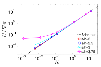
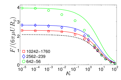
Figure 13: (Left panel) Numerically measured permeability of a slab as a function of the input permeability for different blob-blob spacings $s$. (Right panel) Measured drag (symbols) on a permeable sphere moving inside a fixed impermeable sphere, as a function of the input permeability, for three different resolutions, indicated as the number of blobs on the outer shell (642, 2562 or 10242 blobs) and inner sphere (56, 239 or 1760 blobs, respectively), see legend. The theoretical result based on the geometric radii of the spheres is shown with a dashed black line, while the theoretical result based on the effective hydrodynamic radii in the impermeable limit (which vary with resolution) is shown with a solid line of the same color as the corresponding symbols.

C.1.1 Permeable Slab

First, we compute the flow through a permeable slab to numerically estimate the effective permeability of a rigid multiblob for several spacings between the blobs. We compose a slab of thickness $5s$ from blobs placed on a cubic lattice with spacing $s$ (i.e., the slab has five layers of blobs), and place the slab in the middle of a cubic domain of side $L$. We impose no-slip for the tangential stress (traction) on all boundaries of the domain using the technique developed by Griffith NonProjection_Griffith . For the normal component, on the sides of the domain perpendicular to the slab we impose no-slip, and we impose a pressure jump of magnitude $\Delta\pi$ across the boundaries parallel to the slab. We measure the velocity $U$ of the resulting nearly uniform flow (leak) through the slab as the velocity at the centerline of the slab a quarter of the domain from the left boundary.

At steady state we expect a uniform flow inside the slab with magnitude determined from the Brinkmann equation,

$$\nabla\pi=\frac{\Delta\pi}{L}=-\frac{\eta}{\kappa}U,$$ (40)

where $\kappa$ is the permeability (porosity). In the left panel of Fig. 13 we compare this to the numerical observations. We see that for a variety of spacings between the blobs we get the correct permeability for large target values of $\kappa$. However, as we make the the slab less and less permeable and approach the (singular) impermeable limit, we start to see a small but measurable leak in the rigid multiblob results. This leak is larger the larger the spacing between the blobs is, consistent with the intuition that leak occurs between the blobs. This suggests that for permeable bodies it is better to reduce the spacing between the markers to $s\approx 2h$ as suggested in RigidIBM . Note that the conditioning of the blob-blob mobility matrix is significantly improved for permeable bodies compared to impermeable bodies, so that this reduction in the spacing does not lead to conditioning problems except for very small values of $\kappa$.

C.1.2 Permeable Sphere

Next we examine the translational mobility of a permeable sphere of radius $a$. The drag force on a permeable sphere of radius $R$ moving through an unbounded domain with velocity $U$ is given in BrinkmanSphereAsymptotics ; BrinkmanSphere ,

$$\left(6\pi\eta UR\right)^{-1}F=\frac{G}{1+3G/\left(2\sigma^{2}\right)}=1-\frac{1}{\sigma}+O\left(\frac{1}{\sigma^{2}}\right),$$

where $G=1-\sigma^{-1}\tanh\sigma$ and $\sigma=\sqrt{a^{2}/\kappa}$. To eliminate finite-size effects, and following our prior work RigidIBM for impermeable spheres, we consider here a permeable sphere inside an impermeable spherical shell, that is, we impose a no-slip boundary condition on a spherical shell of radius $b=a/\lambda$ that is concentric to the permeable sphere.

The equations we need to solve are the Stokes equations in the region between the spherical shells and the Brinkman equation (37) inside the permeable sphere, with no-slip boundary conditions on the outer shell and continuity of both velocity and stress on the boundary of the permeable sphere. The drag force can be shown to be

$$\alpha\left(6\pi\eta UR\right)^{-1}F=5\lambda^{5}+G(\sigma)\left[1-\lambda^{5}\left(6+\frac{15}{\sigma^{2}}\right)\right],$$ (41)

where

$$\alpha = 1-5\lambda^{3}+\lambda^{5}\left(9+\frac{15}{2\sigma^{2}}\right)-5\lambda^{6}$$

$$+G(\sigma)\Big{[}\frac{3}{2\sigma^{2}}-\frac{9}{4}\lambda+\frac{15}{2}\lambda^{3}\left(1+\frac{1}{\sigma^{2}}\right)$$

$$-\frac{9}{2}\lambda^{5}\left(\frac{5}{2}+\frac{7}{\sigma^{2}}+\frac{5}{\sigma^{4}}\right)+\lambda^{6}\left(6+\frac{15}{\sigma^{2}}\right)\Big{]}.$$

The solution to this problem in the limit of an impermeable sphere has been computed by Brenner BrennerBook (see Appendix C in RigidIBM for the full solution),

$$\left(6\pi\eta UR\right)^{-1}F=\frac{1-\lambda^{5}}{1-\frac{9}{4}\lambda+\frac{5}{2}\lambda^{3}-\frac{9}{4}\lambda^{5}+\lambda^{6}}.$$ (43)

The outside impermeable fixed shell is constructed as a rigid multiblob using the same recursive triangulation as before. Recall that the inner sphere has to be uniformly filled with blobs for $\kappa>0$; we construct a filled sphere model with typical spacing between nearest-neighbor blobs of $s\approx 2h$ using a tetrahedral mesh generator, starting from a uniform surface triangulation. In the right panel of Fig. 13 we show the drag on the inner sphere compared to the theory (41), for several different resolutions. We observe that for large permeabilities there is an excellent agreement with the theory based on the geometric radii of the inner and outer spheres, even for rather modest resolutions. But for small permeabilities, we see deviations from the theory. This is not unexpected, since in the limit of zero permeability we must converge back to the rigid sphere case, and we know that in this case the drag is determined by the larger effective hydrodynamic and not the geometric radius. Of course, as the resolution is refined we get convergence of the geometric and hydrodynamic radius, but convergence is very slow.

Our numerical observations are consistent with physical intuition. For large permeability, the flow is smooth and there is no jump in the pressure (and velocity derivatives) across the surface of the body, making the rigid multiblob models relatively accurate even for modest resolutions. However, for impermeable bodies the flow develops a boundary layer near the surface of the inner sphere and the pressure and velocity are no longer sufficiently smooth and the accuracy is lowered. We were able to account for the smearing of the no-slip condition for an impermeable (passive) sphere by adjusting the hydrodynamic radius $R_{h}>R_{g}$, but this adjustment cannot be done uniformly for all permeabilities. This is similar to the situation for active spheres discussed in Section IV.3, and highlights the inherent accuracy limitations of regularized methods, including both the rigid multiblob method and the method of regularized Stokeslets.

Appendix D Empirical mobility of a sphere near a wall

A number of theoretical predictions are available for the mobility of a sphere close to a wall BrennerBook (see Appendix D in BrownianMultiBlobs for a summary). However, except for the translational mobility perpendicular to the wall, for which Brenner computed an exact infinite sum Brenner1961 (see SingleWallPerpMobility for an approximate rational fit), the theoretical results are based on asymptotic expansions and have a limited range of validity. Since the dynamics of spherical colloids near a no-slip boundary is relevant to a number of experimental studies, we give here empirical fits to the mobility computed in Section V.1 using a rigid multiblob with 642 blobs (our highest resolution).

We have fitted the mobilities shown in the panels of Fig. 5 with a rational function of the form

$$\frac{\mu(x=H/R_{h})}{\mu^{0}}=\delta+\left(\frac{1}{x}\right)^{\alpha}\,\frac{f_{n,2}x{}^{2}+f_{n,1}x+f_{n,0}}{x^{2}+f_{d,1}x+f_{d,0}},$$

where $\mu^{0}$ is the bulk mobility and $\delta$, $\alpha$ and $f_{n,2}$ have been chosen to ensure the correct leading-order asymptotic scaling for large distances to the wall $H$ and the rest of the constants are fitting parameters. The values of all the coefficients are given in Table 6.

Mobility	$\mu^{0}$	$\delta$	$\alpha$	$f_{n,2}$	$f_{n,1}$	$f_{n,0}$	$f_{d,1}$	$f_{d,0}$	max. relative error
$\mu_{tt}^{\parallel}$	$6\pi\eta R_{h}$	1	1	$-\frac{9}{16}$	0.826024	-0.311607	-1.4297	0.498974	$5.6\cdot 10^{-3}$
$\mu_{rr}^{\parallel}$	$8\pi\eta R_{\tau}^{3}$	1	3	$-\frac{5}{16}$	0.15118	0.0830598	-0.443529	-0.406958	$4.9\cdot 10^{-4}$
$\mu_{rr}^{\perp}$	$8\pi\eta R_{\tau}^{3}$	1	3	$-\frac{1}{8}$	0.122506	-0.0105777	-0.953632	0.0339739	$7.2\cdot 10^{-5}$
$\mu_{rt}^{\parallel}$	$6\pi\eta R_{h}^{2}$	0	4	$\frac{3}{32}$	-0.142813	0.0508471	-0.528495	-0.454638	$6.6\cdot 10^{-3}$

Table 6: Fitting parameters for the mobility of a sphere close to a wall obtained using the numerical mobility of the 642-blob model. In the last column we report the maximum relative error between the numerical mobility and the fit in the interval $(1.03,10)R_{h}$.

References

- (1) Donald L Koch and Ganesh Subramanian. Collective hydrodynamics of swimming microorganisms: Living fluids. Annual Review of Fluid Mechanics, 43:637–659, 2011.
- (2) Somdeb Ghose and R Adhikari. Irreducible representations of oscillatory and swirling flows in active soft matter. Physical review letters, 112(11):118102, 2014.
- (3) Enkeleida Lushi and Charles S Peskin. Modeling and simulation of active suspensions containing large numbers of interacting micro-swimmers. Computers & Structures, 122(0):239 – 248, 2013.
- (4) Blaise Delmotte, Eric E. Keaveny, Franck Plouraboue, and Eric Climent. Large-scale simulation of steady and time-dependent active suspensions with the force-coupling method. Journal of Computational Physics, 302:524 – 547, 2015.
- (5) James W Swan, John F Brady, Rachel S Moore, et al. Modeling hydrodynamic self-propulsion with Stokesian Dynamics. Or teaching Stokesian Dynamics to swim. Physics of Fluids, 23:071901, 2011.
- (6) Ankita Pandey, PB Kumar, and R Adhikari. Flow-induced nonequilibrium self-assembly in suspensions of stiff, apolar, active filaments. arXiv preprint arXiv:1408.0433, 2014.
- (7) Huijun Jiang and Zhonghuai Hou. Hydrodynamic interaction induced spontaneous rotation of coupled active filaments. Soft matter, 10(46):9248–9253, 2014.
- (8) Rajesh Singh, Somdeb Ghose, and R Adhikari. Many-body microhydrodynamics of colloidal particles with active boundary layers. Journal of Statistical Mechanics: Theory and Experiment, 2015(6):P06017, 2015.
- (9) Rajesh Singh and R. Adhikari. Universal hydrodynamic mechanisms for crystallization in active colloidal suspensions. arXiv, 2016.
- (10) R. M. Jendrejack, J. J. de Pablo, and M. D. Graham. Stochastic simulations of DNA in flow: Dynamics and the effects of hydrodynamic interactions. J. Chem. Phys., 116(17):7752–7759, 2002.
- (11) J. P. Hernandez-Ortiz, J. J. de Pablo, and M. D. Graham. Fast Computation of Many-Particle Hydrodynamic and Electrostatic Interactions in a Confined Geometry. Phys. Rev. Lett., 98(14):140602, 2007.
- (12) A. Sierou and J. F. Brady. Accelerated Stokesian Dynamics simulations. J. Fluid Mech., 448:115–146, 2001.
- (13) James W. Swan and John F. Brady. Simulation of hydrodynamically interacting particles near a no-slip boundary. Physics of Fluids, 19(11):113306, 2007.
- (14) K Hinsen. HYDROLIB: a library for the evaluation of hydrodynamic interactions in colloidal suspensions. Computer physics communications, 88(2):327–340, 1995.
- (15) B Cichocki and K Hinsen. Stokes drag on conglomerates of spheres. Physics of Fluids, 7:285, 1995.
- (16) A Ortega, D Amorós, and J García de La Torre. Prediction of hydrodynamic and other solution properties of rigid proteins from atomic-and residue-level models. Biophysical journal, 101(4):892–898, 2011. Code available at http://leonardo.inf.um.es/macromol/programs/hydropro/hydropro.htm.
- (17) José García de la Torre, María L Huertas, and Beatriz Carrasco. Calculation of hydrodynamic properties of globular proteins from their atomic-level structure. Biophysical Journal, 78(2):719–730, 2000.
- (18) Maciej Długosz and Jan M Antosiewicz. Toward an accurate modeling of hydrodynamic effects on the translational and rotational dynamics of biomolecules in many-body systems. The Journal of Physical Chemistry B, 119(26):8425–8439, 2015.
- (19) Richard M Jendrejack, David C Schwartz, Michael D Graham, and Juan J de Pablo. Effect of confinement on DNA dynamics in microfluidic devices. J. Chem. Phys., 119:1165, 2003.
- (20) James W Swan and John F Brady. Particle motion between parallel walls: Hydrodynamics and simulation. Physics of Fluids, 22:103301, 2010.
- (21) James W Swan and John F Brady. The hydrodynamics of confined dispersions. Journal of Fluid Mechanics, 687:254, 2011.
- (22) Anthony JC Ladd, Rahul Kekre, and Jason E Butler. Comparison of the static and dynamic properties of a semiflexible polymer using lattice Boltzmann and Brownian-dynamics simulations. Physical Review E, 80(3):036704, 2009.
- (23) Josephine Ainley, Sandra Durkin, Rafael Embid, Priya Boindala, and Ricardo Cortez. The method of images for regularized stokeslets. Journal of Computational Physics, 227(9):4600–4616, 2008.
- (24) Karin Leiderman, Elizabeth L Bouzarth, Ricardo Cortez, and Anita T Layton. A regularization method for the numerical solution of periodic stokes flow. Journal of Computational Physics, 236:187–202, 2013.
- (25) Dag Lindbo and Anna-Karin Tornberg. Spectrally accurate fast summation for periodic stokes potentials. Journal of Computational Physics, 229(23):8994–9010, 2010.
- (26) Oana Marin, Katarina Gustavsson, and Anna-Karin Tornberg. A highly accurate boundary treatment for confined stokes flow. Computers & Fluids, 66:215–230, 2012.
- (27) Ludvig Af Klinteberg and Anna-Karin Tornberg. Fast ewald summation for stokesian particle suspensions. International Journal for Numerical Methods in Fluids, 76(10):669–698, 2014.
- (28) Juan P Hernández-Ortiz, Juan J de Pablo, and Michael D Graham. method for hydrodynamic interactions of confined polymer systems: Brownian dynamics. The Journal of chemical physics, 125(16):164906, 2006.
- (29) James W Swan and Gang Wang. Rapid calculation of hydrodynamic and transport properties in concentrated solutions of colloidal particles and macromolecules. Physics of Fluids (1994-present), 28(1):011902, 2016.
- (30) Blaise Delmotte and Eric E Keaveny. Simulating brownian suspensions with fluctuating hydrodynamics. The Journal of chemical physics, 143(24):244109, 2015.
- (31) Eligiusz Wajnryb, Krzysztof A Mizerski, Pawel J Zuk, and Piotr Szymczak. Generalization of the rotne–prager–yamakawa mobility and shear disturbance tensors. Journal of Fluid Mechanics, 731:R3, 2013.
- (32) Jens Rotne and Stephen Prager. Variational treatment of hydrodynamic interaction in polymers. The Journal of Chemical Physics, 50:4831, 1969.
- (33) Zhi Liang, Zydrunas Gimbutas, Leslie Greengard, Jingfang Huang, and Shidong Jiang. A fast multipole method for the rotne–prager–yamakawa tensor and its applications. Journal of Computational Physics, 234:133–139, 2013.
- (34) Z. Gimbutas, L. Greengard, and S. Veerapaneni. Simple and efficient representations for the fundamental solutions of Stokes flow in a half-space. Journal of Fluid Mechanics, 776:R1, 2015. Code available at http://www.cims.nyu.edu/cmcl/fmm3dlib/fmm3dlib.html.
- (35) Adolfo Vazquez-Quesada, Florencio Balboa Usabiaga, and Rafael Delgado-Buscalioni. A multiblob approach to colloidal hydrodynamics with inherent lubrication. The Journal of Chemical Physics, 141(20), 2014.
- (36) Kengo Ichiki. Improvement of the stokesian dynamics method for systems with a finite number of particles. Journal of Fluid Mechanics, 452:231–262, 2002. See http://kichiki.github.com/libstokes/ for software.
- (37) C. W. J. Beenakker. Ewald sum of the Rotne-Prager tensor. J. Chem. Phys., 85:1581, 1986.
- (38) Mu Wang and John F Brady. Spectral ewald acceleration of stokesian dynamics for polydisperse suspensions. Journal of Computational Physics, 306:443–477, 2016.
- (39) Fuduo Ma, Xingfu Yang, Hui Zhao, and Ning Wu. Inducing propulsion of colloidal dimers by breaking the symmetry in electrohydrodynamic flow. Phys. Rev. Lett., 115:208302, 2015.
- (40) Jeremie Palacci, Stefano Sacanna, Asher Preska Steinberg, David J Pine, and Paul M Chaikin. Living crystals of light-activated colloidal surfers. Science, 339(6122):936–940, 2013.
- (41) S. Delong, F. Balboa Usabiaga, R. Delgado-Buscalioni, B. E. Griffith, and A. Donev. Brownian Dynamics without Green’s Functions. J. Chem. Phys., 140(13):134110, 2014. Software available at https://github.com/stochasticHydroTools/FIB.
- (42) B. Kallemov, A. Pal Singh Bhalla, B. E. Griffith, and A. Donev. An immersed boundary method for rigid bodies. Communications in Applied Mathematics and Computational Science, 11(1):79–141, 2016. Software available at https://github.com/stochasticHydroTools/RigidBodyIB.
- (43) F. Balboa Usabiaga, R. Delgado-Buscalioni, B. E. Griffith, and A. Donev. Inertial Coupling Method for particles in an incompressible fluctuating fluid. Comput. Methods Appl. Mech. Engrg., 269:139–172, 2014. Code available at https://github.com/fbusabiaga/fluam.
- (44) S. Lomholt and M.R. Maxey. Force-coupling method for particulate two-phase flow: Stokes flow. J. Comp. Phys., 184(2):381–405, 2003.
- (45) Eric E. Keaveny. Fluctuating force-coupling method for simulations of colloidal suspensions. J. Comp. Phys., 269(0):61 – 79, 2014.
- (46) P. J. Atzberger. Stochastic Eulerian-Lagrangian Methods for Fluid-Structure Interactions with Thermal Fluctuations. J. Comp. Phys., 230:2821–2837, 2011.
- (47) Megan S Davies Wykes, Jérémie Palacci, Takuji Adachi, Leif Ristroph, Xiao Zhong, Michael D Ward, Jun Zhang, and Michael J Shelley. Dynamic self-assembly of microscale rotors and swimmers. Soft Matter, 12(20):4584–4589, 2016.
- (48) Ayan Chakrabarty, Andrew Konya, Feng Wang, Jonathan V Selinger, Kai Sun, and Qi-Huo Wei. Brownian motion of boomerang colloidal particles. Physical review letters, 111(16):160603, 2013.
- (49) Ayan Chakrabarty, Andrew Konya, Feng Wang, Jonathan V. Selinger, Kai Sun, and Qi-Huo Wei. Brownian motion of arbitrarily shaped particles in two dimensions. Langmuir, 30(46):13844–13853, 2014.
- (50) Mu Wang and John F Brady. Short-time transport properties of bidisperse suspensions and porous media: A stokesian dynamics study. The Journal of chemical physics, 142(9):094901, 2015.
- (51) Tri T Pham, Ulf D Schiller, J Ravi Prakash, and Burkhard Dünweg. Implicit and explicit solvent models for the simulation of a single polymer chain in solution: Lattice boltzmann versus brownian dynamics. J. Chem. Phys., 131:164114, 2009.
- (52) Rahul Kekre, Jason E. Butler, and Anthony J. C. Ladd. Comparison of lattice-Boltzmann and Brownian-dynamics simulations of polymer migration in confined flows. Phys. Rev. E, 82:011802, 2010.
- (53) Adolfo J Banchio and John F Brady. Accelerated stokesian dynamics: Brownian motion. The Journal of chemical physics, 118:10323, 2003.
- (54) B. Cichocki, B. U. Felderhof, K. Hinsen, E. Wajnryb, and J. Blawzdziewicz. Friction and mobility of many spheres in stokes flow. The Journal of Chemical Physics, 100(5):3780–3790, 1994.
- (55) B. Cichocki, R. B. Jones, Ramzi Kutteh, and E. Wajnryb. Friction and mobility for colloidal spheres in stokes flow near a boundary: The multipole method and applications. The Journal of Chemical Physics, 112(5):2548–2561, 2000.
- (56) Anthony JC Ladd. Hydrodynamic interactions in a suspension of spherical particles. The Journal of chemical physics, 88(8):5051–5063, 1988.
- (57) Anthony JC Ladd. Hydrodynamic transport coefficients of random dispersions of hard spheres. The Journal of Chemical Physics, 93(5):3484–3494, 1990.
- (58) Daisuke Takagi, Adam B Braunschweig, Jun Zhang, and Michael J Shelley. Dispersion of self-propelled rods undergoing fluctuation-driven flips. Phys. Rev. Lett., 110(3):038301, 2013.
- (59) E. Nazockdast, A. Rahimian, D. Zorin, and M. Shelley. A fast platform for simulating flexible fiber suspensions applied to cell mechanics. Preprint ArXiv:1602.05650, 2016.
- (60) Miguel X Fernandes and José García de la Torre. Brownian dynamics simulation of rigid particles of arbitrary shape in external fields. Biophysical journal, 83(6):3039–3048, 2002.
- (61) Simón Poblete, Adam Wysocki, Gerhard Gompper, and Roland G. Winkler. Hydrodynamics of discrete-particle models of spherical colloids: A multiparticle collision dynamics simulation study. Phys. Rev. E, 90:033314, 2014.
- (62) Vladimir Lobaskin and Burkhard Dünweg. A new model for simulating colloidal dynamics. New Journal of Physics, 6(1):54, 2004.
- (63) John J Molina and Ryoichi Yamamoto. Direct numerical simulations of rigid body dispersions. i. mobility/friction tensors of assemblies of spheres. The Journal of chemical physics, 139(23):234105, 2013.
- (64) Ramzi Kutteh. Rigid body dynamics approach to stokesian dynamics simulations of nonspherical particles. J. Chem. Phys., 132(17):–, 2010.
- (65) T.T. Bringley and C.S. Peskin. Validation of a simple method for representing spheres and slender bodies in an immersed boundary method for Stokes flow on an unbounded domain. J. Comp. Phys., 227(11):5397–5425, 2008.
- (66) M Zurita-Gotor, J Bławzdziewicz, and E Wajnryb. Motion of a rod-like particle between parallel walls with application to suspension rheology. Journal of Rheology, 51(1):71–97, 2007.
- (67) Ricardo Cortez, Lisa Fauci, and Alexei Medovikov. The method of regularized Stokeslets in three dimensions: analysis, validation, and application to helical swimming. Physics of Fluids, 17:031504, 2005.
- (68) S. Delong, F. Balboa Usabiaga, and A. Donev. Brownian dynamics of confined rigid bodies. J. Chem. Phys., 143(14), 2015. Software available at https://github.com/stochasticHydroTools/RotationalDiffusion.
- (69) A. Donev and E. Vanden-Eijnden. Dynamic Density Functional Theory with hydrodynamic interactions and fluctuations. J. Chem. Phys., 140(23):234115, 2014.
- (70) Krzysztof A Mizerski, Eligiusz Wajnryb, Pawel J Zuk, and Piotr Szymczak. The rotne-prager-yamakawa approximation for periodic systems in a shear flow. The Journal of chemical physics, 140(18):184103, 2014.
- (71) Erik M Gauger, Matthew T Downton, and Holger Stark. Fluid transport at low reynolds number with magnetically actuated artificial cilia. The European Physical Journal E, 28(2):231–242, 2009.
- (72) JR Blake. A note on the image system for a stokeslet in a no-slip boundary. In Proc. Camb. Phil. Soc, volume 70, pages 303–310. Cambridge Univ Press, 1971.
- (73) S Bhattacharya, J Blawzdziewicz, and E Wajnryb. Hydrodynamic interactions of spherical particles in suspensions confined between two planar walls. Journal of Fluid Mechanics, 541:263–292, 2005.
- (74) David J Smith. A boundary element regularized stokeslet method applied to cilia-and flagella-driven flow. In Proceedings of the Royal Society of London A: Mathematical, Physical and Engineering Sciences, volume 465, pages 3605–3626. The Royal Society, 2009.
- (75) Thomas D Montenegro-Johnson, Sebastien Michelin, and Eric Lauga. A regularised singularity approach to phoretic problems. arXiv preprint arXiv:1511.03078, 2015.
- (76) Blaise Delmotte, Eric Climent, and Franck Plouraboué. A general formulation of bead models applied to flexible fibers and active filaments at low reynolds number. Journal of Computational Physics, 286:14–37, 2015.
- (77) Constantine Pozrikidis. Boundary integral and singularity methods for linearized viscous flow. Cambridge University Press, 1992.
- (78) Harper Langston, Leslie Greengard, and Denis Zorin. A free-space adaptive fmm-based pde solver in three dimensions. Communications in Applied Mathematics and Computational Science, 6(1):79–122, 2011. Software available at https://github.com/dmalhotra/pvfmm.
- (79) Amina Bouras and Valérie Frayssé. Inexact matrix-vector products in krylov methods for solving linear systems: A relaxation strategy. SIAM Journal on Matrix Analysis and Applications, 26(3):660–678, 2005.
- (80) Simon K Layton and Lorena A Barba. Inexact krylov iterations and relaxation strategies with fast-multipole boundary element method. arXiv preprint arXiv:1506.05957, 2015. Software available at https://github.com/barbagroup/fmm-bem-relaxed.
- (81) Satish Balay, William D. Gropp, Lois Curfman McInnes, and Barry F. Smith. Efficient management of parallelism in object oriented numerical software libraries. In E. Arge, A. M. Bruaset, and H. P. Langtangen, editors, Modern Software Tools in Scientific Computing, pages 163–202. Birkhäuser Press, 1997. Software available at http://www.mcs.anl.gov/petsc.
- (82) P. J. Atzberger. A note on the correspondence of an immersed boundary method incorporating thermal fluctuations with Stokesian-Brownian dynamics. Physica D: Nonlinear Phenomena, 226(2):144–150, 2007.
- (83) C.S. Peskin. The immersed boundary method. Acta Numerica, 11:479–517, 2002.
- (84) M. R. Maxey and B. K. Patel. Localized force representations for particles sedimenting in Stokes flow. International journal of multiphase flow, 27(9):1603–1626, 2001.
- (85) B.E. Griffith. An accurate and efficient method for the incompressible Navier-Stokes equations using the projection method as a preconditioner. J. Comp. Phys., 228(20):7565–7595, 2009.
- (86) Ricardo Cortez. The method of regularized stokeslets. SIAM Journal on Scientific Computing, 23(4):1204–1225, 2001.
- (87) B.E. Griffith, R.D. Hornung, D.M. McQueen, and C.S. Peskin. An adaptive, formally second order accurate version of the immersed boundary method. J. Comput. Phys., 223(1):10–49, 2007. Software available at https://github.com/ibamr/ibamr.
- (88) Yuanxun Bao, Jason Kaye, and Charles S. Peskin. A gaussian-like immersed-boundary kernel with three continuous derivatives and improved translational invariance. Journal of Computational Physics, 316:139 – 144, 2016. Software available at https://github.com/stochasticHydroTools/IBMethod.
- (89) M. Cai, A. J. Nonaka, J. B. Bell, B. E. Griffith, and A. Donev. Efficient Variable-Coefficient Finite-Volume Stokes Solvers. Comm. in Comp. Phys. (CiCP), 16(5):1263–1297, 2014.
- (90) Howard C Elman, David J Silvester, and Andrew J Wathen. Finite elements and fast iterative solvers: with applications in incompressible fluid dynamics. Oxford University Press, 2014.
- (91) Howard Elman, Victoria E Howle, John Shadid, Robert Shuttleworth, and Ray Tuminaro. Block preconditioners based on approximate commutators. SIAM Journal on Scientific Computing, 27(5):1651–1668, 2006.
- (92) R. Falgout, J. Jones, and U. Yang. The design and implementation of hypre, a library of parallel high performance preconditioners. Numerical solution of partial differential equations on parallel computers, pages 267–294, 2006. Software available at http://www.llnl.gov/CASC/hypre.
- (93) Yousef Saad. Iterative methods for sparse linear systems. SIAM, 2003.
- (94) A.J.C. Ladd. Numerical simulations of particulate suspensions via a discretized Boltzmann equation. II. Numerical results. Journal of Fluid Mechanics, 271(1):311–339, 1994.
- (95) Reghan J Hill, Donald L Koch, and Anthony JC Ladd. Moderate-reynolds-number flows in ordered and random arrays of spheres. Journal of Fluid Mechanics, 448:243–278, 2001.
- (96) Howard Brenner. The slow motion of a sphere through a viscous fluid towards a plane surface. Chemical Engineering Science, 16(3-4):242 – 251, 1961.
- (97) D. J. Jeffrey and Y. Onishi. Calculation of the resistance and mobility functions for two unequal rigid spheres in low-reynolds-number flow. Journal of Fluid Mechanics, 139:261–290, 2 1984.
- (98) Howard A. Stone and Aravinthan D. T. Samuel. Propulsion of microorganisms by surface distortions. Phys. Rev. Lett., 77:4102–4104, 1996.
- (99) L Durlofsky and JF Brady. Analysis of the brinkman equation as a model for flow in porous media. Physics of Fluids, 30(11):3329–3341, 1987.
- (100) Miroslav Rozlozník and Valeria Simoncini. Krylov subspace methods for saddle point problems with indefinite preconditioning. SIAM journal on matrix analysis and applications, 24(2):368–391, 2002.
- (101) Andreas Klöckner, Nicolas Pinto, Yunsup Lee, B. Catanzaro, Paul Ivanov, and Ahmed Fasih. PyCUDA and PyOpenCL: A Scripting-Based Approach to GPU Run-Time Code Generation. Parallel Computing, 38(3):157–174, 2012.
- (102) AJ Goldman, Raymond G Cox, and Howard Brenner. Slow viscous motion of a sphere parallel to a plane wall - I Motion through a quiescent fluid. Chemical engineering science, 22(4):637–651, 1967.
- (103) Luc P. Faucheux and Albert J. Libchaber. Confined brownian motion. Phys. Rev. E, 49:5158–5163, 1994.
- (104) John Happel and Howard Brenner. Low Reynolds number hydrodynamics: with special applications to particulate media, volume 1. Springer Science & Business Media, 1983.
- (105) Joseph B Keller and Sol I Rubinow. Slender-body theory for slow viscous flow. Journal of Fluid Mechanics, 75(04):705–714, 1976.
- (106) Jeffrey F Trahan and RG Hussey. The stokes drag on a horizontal cylinder falling toward a horizontal plane. Physics of Fluids (1958-1988), 28(10):2961–2967, 1985.
- (107) DJ Jeffrey and Y Onishi. The slow motion of a cylinder next to a plane wall. The Quarterly Journal of Mechanics and Applied Mathematics, 34(2):129–137, 1981.
- (108) DF Katz, JR Blake, and SL Paveri-Fontana. On the movement of slender bodies near plane boundaries at low reynolds number. Journal of Fluid Mechanics, 72(03):529–540, 1975.
- (109) NJ De Mestre and WB Russel. Low-reynolds-number translation of a slender cylinder near a plane wall. Journal of Engineering Mathematics, 9(2):81–91, 1975.
- (110) A. Donev, J. Burton, F. H. Stillinger, and S. Torquato. Tetratic Order in the Phase Behavior of a Hard-Rectangle System. Phys. Rev. B, 73:054109, 2006.
- (111) Alexandre M Roma, Charles S Peskin, and Marsha J Berger. An adaptive version of the immersed boundary method. J. Comput. Phys., 153(2):509–534, 1999.
- (112) Ayan Chakrabarty, Feng Wang, Chun-Zhen Fan, Kai Sun, and Qi-Huo Wei. High-precision tracking of brownian boomerang colloidal particles confined in quasi two dimensions. Langmuir, 29(47):14396–14402, 2013. PMID: 24171648.
- (113) Thorben Benesch, Sotira Yiacoumi, and Costas Tsouris. Brownian motion in confinement. Phys. Rev. E, 68:021401, 2003.
- (114) José M García Bernal, De La Torre, and José García. Transport properties and hydrodynamic centers of rigid macromolecules with arbitrary shapes. Biopolymers, 19(4):751–766, 1980.
- (115) A. Donev, S. Torquato, and F. H. Stillinger. Neighbor List Collision-Driven Molecular Dynamics Simulation for Nonspherical Particles: I. Algorithmic Details II. Applications to Ellipses and Ellipsoids. J. Comp. Phys., 202(2):737–764, 765–793, 2005. code available at http://cims.nyu.edu/~donev/Packing/PackLSD/Instructions.html.
- (116) Anthony JC Ladd. Sedimentation of homogeneous suspensions of non-brownian spheres. Physics of Fluids, 9(3):491–499, 1997.
- (117) John F Brady and Louis J Durlofsky. The sedimentation rate of disordered suspensions. Physics of Fluids, 31(4):717–727, 1988.
- (118) John F Brady, Ronald J Phillips, Julia C Lester, and Georges Bossis. Dynamic simulation of hydrodynamically interacting suspensions. Journal of Fluid Mechanics, 195:257–280, 1988.
- (119) Anthony JC Ladd. Dynamical simulations of sedimenting spheres. Physics of Fluids A: Fluid Dynamics (1989-1993), 5(2):299–310, 1993.
- (120) Nhan-Quyen Nguyen and Anthony JC Ladd. Sedimentation of hard-sphere suspensions at low reynolds number. Journal of Fluid Mechanics, 525:73–104, 2005.
- (121) Yu Zhang, Juan J de Pablo, and Michael D Graham. An immersed boundary method for brownian dynamics simulation of polymers in complex geometries: Application to dna flowing through a nanoslit with embedded nanopits. The Journal of Chemical Physics, 136:014901, 2012.
- (122) Trushant Majmudar, Eric E Keaveny, Jun Zhang, and Michael J Shelley. Experiments and theory of undulatory locomotion in a simple structured medium. Journal of The Royal Society Interface, 9(73):1809–1823, 2012.
- (123) Kyongmin Yeo and Martin R Maxey. Dynamics of concentrated suspensions of non-colloidal particles in couette flow. Journal of Fluid Mechanics, 649(1):205–231, 2010.
- (124) Boyce E Griffith and Xiaoyu Luo. Hybrid finite difference/finite element version of the immersed boundary method. Submitted in revised form, 2012.
- (125) Pat Plunkett, Jonathan Hu, Christopher Siefert, and Paul J Atzberger. Spatially adaptive stochastic methods for fluid–structure interactions subject to thermal fluctuations in domains with complex geometries. Journal of Computational Physics, 277:121–137, 2014.
- (126) E. J. Hinch. Application of the Langevin equation to fluid suspensions. J. Fluid Mech., 72(03):499–511, 1975.
- (127) J. N. Roux. Brownian particles at different times scales: a new derivation of the Smoluchowski equation. Phys. A, 188:526–552, 1992.
- (128) F. Balboa Usabiaga, J. B. Bell, R. Delgado-Buscalioni, A. Donev, T. G. Fai, B. E. Griffith, and C. S. Peskin. Staggered Schemes for Fluctuating Hydrodynamics. SIAM J. Multiscale Modeling and Simulation, 10(4):1369–1408, 2012.
- (129) M. Hütter and H.C. Öttinger. Fluctuation-dissipation theorem, kinetic stochastic integral and efficient simulations. J. Chem. Soc., Faraday Trans., 94(10):1403–1405, 1998.
- (130) Eric E Keaveny and Michael J Shelley. Applying a second-kind boundary integral equation for surface tractions in stokes flow. Journal of Computational Physics, 230(5):2141–2159, 2011.
- (131) HC Brinkman. A calculation of the viscous force exerted by a flowing fluid on a dense swarm of particles. Applied Scientific Research, 1(1):27–34, 1949.
- (132) Gustavo C. Abade, Bogdan Cichocki, Maria L. Ekiel-Jezewska, Gerhard Nagele, and Eligiusz Wajnryb. Short-time dynamics of permeable particles in concentrated suspensions. The Journal of Chemical Physics, 132(1), 2010.
- (133) JJL Higdon and M Kojima. On the calculation of stokes’ flow past porous particles. International Journal of Multiphase Flow, 7(6):719–727, 1981.
- (134) BU Felderhof. Frictional properties of dilute polymer solutions: III. Translational-friction coefficient. Physica A: Statistical Mechanics and its Applications, 80(1):63–75, 1975.
- (135) Peter Huang and Kenneth S Breuer. Direct measurement of anisotropic near-wall hindered diffusion using total internal reflection velocimetry. Physical review E, 76(4):046307, 2007.