Large-Dimensional Dynamic Factor Models: Estimation of Impulse-Response Functions with $I(1)$ Cointegrated Factors

Abstract

We study a large-dimensional Dynamic Factor Model where: (i) the vector of factors $\mathbf{F}_{t}$ is $I(1)$ and driven by a number of shocks that is smaller than the dimension of $\mathbf{F}_{t}$; and, (ii) the idiosyncratic components are either $I(1)$ or $I(0)$. Under (i), the factors $\mathbf{F}_{t}$ are cointegrated and can be modeled as a Vector Error Correction Model (VECM). Under (i) and (ii), we provide consistent estimators, as both the cross-sectional size $n$ and the time dimension $T$ go to infinity, for the factors, the loadings, the shocks, the coefficients of the VECM and therefore the Impulse-Response Functions (IRF) of the observed variables to the shocks. Furthermore: possible deterministic linear trends are fully accounted for, and the case of an unrestricted VAR in the levels $\mathbf{F}_{t}$, instead of a VECM, is also studied. The finite-sample properties the proposed estimators are explored by means of a MonteCarlo exercise. Finally, we revisit two distinct and widely studied empirical applications. By correctly modeling the long-run dynamics of the factors, our results partly overturn those obtained by recent literature. Specifically, we find that: (i) oil price shocks have just a temporary effect on US real activity; and, (ii) in response to a positive news shock, the economy first experiences a significant boom, and then a milder recession.

JEL subject classification: C0, C01, E0.

Key words and phrases: Dynamic Factor models, unit root processes, cointegration, impulse-response functions.

1 Introduction

Since the early 2000s large-dimensional Dynamic Factor Models (DFM) have become increasingly popular in the econometric and macroeconomic literature, and they are nowadays commonly used by policy institutions. They have been extensively used in policy analysis based on impulse-response functions (IRF) (Giannone et al., 2005; Forni et al., 2009; Eickmeier, 2009; Forni and Gambetti, 2010; Barigozzi et al., 2014; Forni et al., 2014; Juvenal and Petrella, 2015; Luciani, 2015; Dahlhaus, 2017), in forecasting (Stock and Watson, 2002; Forni et al., 2005; Giannone et al., 2008; Luciani, 2014; Forni et al., 2018), and in the construction of both business cycle indicators and inflation indexes (Cristadoro et al., 2005; Altissimo et al., 2010).

Starting with a large dataset of macroeconomic variables, DFMs are based on the idea that all the variables in the dataset are driven by a small number of common shocks, their residual dynamics being explained by idiosyncratic components. The common shocks, which are pervasive, i.e., they affect all the variables in the dataset, are interpreted as the macroeconomic shocks. The idiosyncratic components, which are specific to one or a few variables, are interpreted as (a) local or sectoral shocks, or (b) measurement errors; hence they are of little interest in macroeconomic analysis.

Formally, each variable in the $n$-dimensional dataset $x_{it},\ i=1,\ldots,n$, is decomposed into the sum of two unobservable components: the common component $\chi_{it}$, and the idiosyncratic component $\xi_{it}$ (Forni et al., 2000; Forni and Lippi, 2001; Stock and Watson, 2002; Bai, 2003). Moreover, the common components are linear combinations of an $r$-dimensional vector of common factors $\mathbf{F}_{t}=(F_{1t}\ \cdots\ F_{rt})^{\prime}$,

$$x_{it} =\chi_{it}+\xi_{it},$$ (1)

$$\chi_{it} =\lambda_{i1}F_{1t}+\lambda_{i2}F_{2t}+\cdots+\lambda_{ir}F_{rt}=\bm{\lambda}_{i}^{\prime}\mathbf{F}_{t},$$ (2)

where $\bm{\lambda}_{i}=(\lambda_{i1}\ \cdots\ \lambda_{ir})^{\prime}$.

Most of the variables contained in macroeconomic datasets are non-stationary; hence, the factors, and, possibly, also the idiosyncratic components, are non-stationary. When the factors are non-stationary, it holds that

$$\Delta\mathbf{F}_{t}=\mathbf{C}(L)\mathbf{u}_{t},$$ (3)

where $\mathbf{C}(L)$ is an $r\times q$ square-summable matrix in the lag operator, and $\mathbf{u}_{t}=(u_{1t}\ \cdots\ u_{qt})^{\prime}$ is a $q$-dimensional orthonormal white-noise vector of common shocks.

The goal of this paper is to estimate the IRFs of the common components $\chi_{it}$, and therefore of the variables $x_{it}$, to the common shocks $\mathbf{u}_{t}$ in the non-stationary DFM defined by (1)–(3), i.e., to estimate $\bm{\lambda}_{i}^{\prime}\frac{\mathbf{C}(L)}{1-L}$. Specifically, we consider the general case in which: (i) the factors are $I(1)$, singular, and cointegrated, (ii) the idiosyncratic components are either $I(1)$ or $I(0)$, and (iii) the presence of deterministic linear trends is explicitly taken into account. As we discuss in Section 2, all these are relevant features in macroeconomic datasets.

The common practice in the applied DFM literature consists in taking first differences of the non-stationary variables $x_{it}$, thus obtaining a stationary dataset $\Delta x_{it}$ with stationary factors $\Delta\mathbf{F}_{t}$, and then applying principal components to $\Delta x_{it}$, which yields consistent estimates of $\Delta\mathbf{F}_{t}$ and the loadings $\bm{\lambda}_{i}$. An estimate of $\mathbf{C}(L)$ and $\mathbf{u}_{t}$ is then obtained by estimating a VAR for $\Delta\mathbf{F}_{t}$, see e.g., Forni et al. (2009). Finally, all the identification techniques, based on macroeconomic theory, that are used in Structural VAR analysis (SVAR) can be applied also in the DFM setting with no modification to obtain structural shocks and IRFs—see for example Forni et al. (2009), Bai and Wang (2015), and Stock and Watson (2016).

However, it is well known that if the factors are cointegrated, then a VAR for $\Delta\mathbf{F}_{t}$ is not an admissible representation. Rather, we should write a Vector Error Correction Model (VECM) for $\mathbf{F}_{t}$, i.e., a VAR for $\mathbf{F}_{t}$ with $r-c$ unit roots, where $c$ is the cointegration rank of $\mathbf{F}_{t}$. Therefore, in order to obtain consistent estimates of the IRFs we need to consider estimation of a DFM with $I(1)$ cointegrated factors.

The crucial question then is: are the factors likely to be cointegrated? The answer is “yes,” and there are two main reasons why this is the case. Firstly, as predicted by macroeconomic theory, some of the macroeconomic shocks $\mathbf{u}_{t}$ permanently affect the economy (e.g., technological shocks), while some others (such as monetary policy shocks or oil price shocks) have only transitory effects. In other words, in (3) the matrix $\mathbf{C}(1)$ is likely to have reduced rank, which is equivalent to saying that the common factors are cointegrated.

Secondly, Barigozzi et al. (2020) show that if $\mathbf{F}_{t}$ is a singular stochastic vector—i.e., $r$, the dimension of $\mathbf{F}_{t}$, is greater than $q$, the dimension of $\mathbf{u}_{t}$—then the common factors are cointegrated with cointegration rank $c=r-q+d$, where $0\leq d<q$, so that the cointegration rank is at least $r-q$. Moreover, under the assumption that the entries of $\mathbf{C}(L)$ are rational functions of $L$, $\mathbf{F}_{t}$ has the VECM representation:

$$\mathbf{G}(L)\Delta\mathbf{F}_{t}+\bm{\alpha}\bm{\beta}^{\prime}\mathbf{F}_{t-1}=\mathbf{h}+\mathbf{K}\mathbf{u}_{t},$$ (4)

where $\bm{\alpha}$ and $\bm{\beta}$ are both $r\times c$ and full rank, $\mathbf{K}$ is $r\times q$, and $\mathbf{G}(L)$ is a finite-degree matrix polynomial. Therefore, it is legitimate to ask: are the factors likely to be singular? Once again, the answer is “yes.” Indeed, as pointed out in several papers, e.g., Bai and Ng (2007), Forni et al. (2009), and Stock and Watson (2016), equation (2) is just a convenient static representation derived from a “deeper” set of dynamic equations linking the common components $\chi_{it}$ to the common shocks $\mathbf{u}_{t}$. Moreover, singularity of $\mathbf{F}_{t}$ is strongly supported by empirical evidence, see, e.g., Giannone et al. (2005), Amengual and Watson (2007), Forni and Gambetti (2010), Luciani (2015) for US macroeconomic databases, Barigozzi et al. (2014) for the euro area.

So far, the literature has proved consistency (and derived the rate of convergence) for an estimator of the IRFs for DFMs when either the variables are stationary or can be transformed to stationarity by differencing, i.e., when the factors are not cointegrated (Forni et al., 2009). However, the literature has not studied estimation of IRFs when the factors are cointegrated, which, as argued above, is a relevant empirical case in macroeconomics. Our paper fills this gap by proposing two estimators.

A. Having estimated the loadings $\bm{\lambda}_{i}$ and the factors $\mathbf{F}_{t}$, the first estimator is obtained by fitting a VECM as in (4) on the estimated factors. We show that, as $n,T\to\infty$ our estimator of the IRFs is consistent and converges with a rate that not only depends on $n$ and $T$, but also on the number of idiosyncratic components that are $I(1)$, and on the number of variables for which a deterministic trend is present.

B. As an alternative to the estimator of the IRFs based on the VECM, we prove consistency of the IRFs obtained by means of an unrestricted VAR in the levels for the estimated factors. Like in the standard VAR analysis, this approach is consistent at each given lag but it does not provide consistent estimates of the long-run features of the IRFs, see also Phillips (1998). This result is corroborated by a numerical exercise in which the VECM and the unrestricted VAR performances are close at short horizons, whereas at long horizons, the VECM performs better.

Both our estimator of the loadings, which is based on principal component analysis on differenced data, and our estimator of the factors are closely related to those proposed by Bai and Ng (2004). However, our estimator of the factors, although asymptotically equivalent to the one proposed by Bai and Ng (2004), has important finite sample differences owing to a different estimation of the trend slope. A numerical comparison shows that our estimator of the factors tends to perform better than the one proposed by Bai and Ng (2004) for estimation of IRFs.

Our results can be applied, with minor modifications, also to a Factor Augmented VAR (FAVAR) (Bernanke et al., 2005; Bai and Ng, 2006) with $I(1)$ variables. Indeed, FAVARs are equivalent to a restricted version of DFMs (Stock and Watson, 2016).

The potential advantages of our proposed approach are illustrated by means of two empirical applications. In the first application, we study the effects of oil price shocks on the US economy. We compare the IRFs estimated with a non-stationary DFM, as proposed in this paper, with those obtained by Stock and Watson (2016) with a stationary DFM, and we show that once we account for cointegration in the common factors, the estimate of the long-run effects of an oil price shock changes dramatically. Indeed, while Stock and Watson (2016) estimate that oil price shocks have persistent effects on the US economy, we find that the effects of an oil price shock vanish after five to eight years, a finding consistent with the idea that only technological shocks are capable of having a permanent effect on the real side of the economy.

In the second empirical application, we study the effects of news shocks on the US economy. To do so, we compare the IRFs estimated with a non-stationary FAVAR, where the factors are either extracted as proposed in this paper, or as proposed by Forni et al. (2014), i.e., under the assumption that all the idiosyncratic components are $I(0)$. The IRFs obtained with our approach partly overturn the results in Forni et al. (2014) in that we find that in response to a positive news shock, hours worked respond positively, and the economy experiences a significant boom, and then a milder recession.

Lastly, let us mention that our non-stationary DFM has recently been used by Alessi and Kerssenfischer (2019) to study the response of asset prices to monetary policy shocks. When estimated using a standard SVAR, the response is very slow and not statistically significant. However, by using our non-stationary DFM, Alessi and Kerssenfischer (2019) find strong and quick asset price reactions, both on euro area and US data.

The paper is organized as follows. In Section 2 we present the model and its assumptions. Section 3 establishes consistency and rates for our estimators of the IRFs. In Section 4 we propose an information criterion to determine the number of permanent shocks $q-d$, which allows us to infer the cointegration rank of the factors. In Section 5, by means of a MonteCarlo simulation exercise, we study the finite sample properties of our estimators. Finally, in Section 6 we apply our methodology to a US quarterly macroeconomic dataset and in two separate exercises we study the impact of oil price and of news shocks. In Section 7 we conclude. The proofs of our main results are in Appendix A. A complementary appendix contains the proofs of all lemmas, details on identification of the IRFs, a comparison with FAVARs, and additional numerical results.

2 The non-stationary Dynamic Factor model

2.1 $I(1)$ vectors and cointegration

Throughout the paper, we will adopt the following definitions for $I(0)$, $I(1)$, and cointegrated stochastic vectors. They are standard and hold both for non-singular vectors, as in all textbooks (see, e.g., Johansen, 1995, Ch. 3), and for singular vectors.

1. Consider an $r\times q$ matrix $\mathbf{A}(L)=\mathbf{A}_{0}+\mathbf{A}_{1}L+\cdots,$ with the assumption that the series $\sum_{j=0}^{\infty}\mathbf{A}_{j}z^{j}$ converges for all complex number $z$ such that $|z|<1+\delta$ for some $\delta>0$. This condition is fulfilled when the entries of $\mathbf{A}(L)$ are rational functions of $L$ with no poles inside or on the unit circle (the VARMA case). Given the $r$-dimensional stationary stochastic vector

   $$\mathbf{z}_{t}=\mathbf{A}(L)\mathbf{v}_{t},$$

   where $\mathbf{v}_{t}$ is a $q$-dimensional white noise, $q\leq r$, we say that $\mathbf{z}_{t}$ is $I(0)$ if $\mathbf{A}(1)\neq\mathbf{0}$.

2. The $r$ dimensional stochastic vector $\mathbf{z}_{t}$ is $I(1)$ if $\Delta\mathbf{z}_{t}$ is $I(0)$.

3. The $r$-dimensional $I(1)$ vector $\mathbf{z}_{t}$ is cointegrated of order $c$, $0<c<r$, if (1) there exist linearly independent $r$-dimensional vectors $\bm{\beta}_{k}$, $k=1,\ldots,c$, such that $\bm{\beta}_{k}^{\prime}\mathbf{z}_{t}$ is stationary, (2) if $\bm{\gamma}^{\prime}\mathbf{z}_{t}$ is stationary then $\bm{\gamma}$ is a linear combination of the vectors $\bm{\beta}_{k}$.

Some important properties for our model follow from these definitions.

Remark 1

2. Some of the coordinates of an $I(1)$ vector can be stationary.

3. If one of the coordinates of the $I(1)$ vector $\mathbf{z}_{t}$ is stationary, then $\mathbf{z}_{t}$ is cointegrated.

4. The cointegration rank of $\mathbf{z}_{t}$ is equal to $r$ minus the rank of $\mathbf{A}(1)$.

5. It easy to see that $\mathbf{z}_{t}$ is cointegrated with cointegration rank $c$ if and only if $\mathbf{z}_{t}$ can be linearly transformed into a vector whose first $c$ coordinates are stationary and the remaining $r-c$ are $I(1)$. For, let $\mathbf{z}_{t}$ be cointegrated of order $c$ with cointegration vectors $\bm{\beta}_{k}$, $k=1,\ldots,c$. Let $\bm{\beta}=(\bm{\beta}_{1}\ \cdots\ \bm{\beta}_{c})$ and $\mathbf{B}=(\bm{\beta}\ \ \bm{\beta}_{\perp})$, where $\bm{\beta}_{\perp}$ is an $r\times(r-c)$ matrix whose columns are linearly independent and orthogonal to the columns of $\bm{\beta}$. Then, the first $c$ coordinates of $\mathbf{z}^{*}_{t}=\mathbf{B}^{\prime}\mathbf{z}_{t}$ are stationary while the remaining $r-c$ are $I(1)$.

6. Note that if $\mathbf{z}_{t}$ is $I(1)$ and $r>q$, then obviously $\mathbf{z}_{t}$ is cointegrated with cointegration rank at least $r-q$, that is, $c=(r-q)+d$ with $0\leq d<q$.

2.2 Assumptions on common and idiosyncratic components

Define $\mathbf{x}_{t}=(x_{1t}\ \cdots\ x_{nt})^{\prime}$, $\bm{\chi}_{t}=(\chi_{1t}\ \cdots\ \chi_{nt})^{\prime}$, $\bm{\xi}_{t}=(\xi_{1t}\ \cdots\ \xi_{nt})^{\prime}$, $\bm{\Lambda}=(\bm{\lambda}_{1}\ \cdots\ \bm{\lambda}_{n})^{\prime}$. Then, the non-stationary DFM that we consider in this paper and given in equations (1) and (3) become:

$$\mathbf{x}_{t} =\bm{\chi}_{t}+\bm{\xi}_{t}=\bm{\Lambda}\mathbf{F}_{t}+\bm{\xi}_{t},$$ (5)

$$\Delta\mathbf{F}_{t} =\mathbf{C}(L)\mathbf{u}_{t}.$$ (6)

Firstly, we suppose that $\mathbf{F}_{t}$ has two equivalent representations: an ARIMA and a VECM. Specifically, we assume the following.

Assumption 1

(Common shocks and common factors)

1. $\mathbf{u}_{t}=(u_{1t}\ \cdots\ u_{qt})^{\prime}$ is a strong orthonormal $q$-dimensional vector white noise, i.e., $\mathsf{E}[\mathbf{u}_{t}]=\mathbf{0}_{q}$, $\mathsf{E}[\mathbf{u}_{t}\mathbf{u}_{t}^{\prime}]=\mathbf{I}_{q}$, and $\mathbf{u}_{t}$ and $\mathbf{u}_{t-k}$ are independent for any $k\neq 0$, moreover $\mathsf{E}[u_{jt}^{4}]\leq M_{1}$, for some positive real $M_{1}$ independent of $j$.

2. The $r$-dimensional stochastic vector $\mathbf{F}_{t}$ is $I(1)$ and has the ARIMA representation

   $$\mathbf{S}(L)\Delta\mathbf{F}_{t}=\mathbf{Q}(L)\mathbf{u}_{t},$$ (7)

   where: (i) $\mathbf{S}(L)$ is an $r\times r$ finite-degree matrix polynomial with $\det(\mathbf{S}(z))\neq 0$ for $|z|\leq 1$; (ii) $\mathbf{S}(0)=\mathbf{I}_{r}$; (iii) $\mathbf{Q}(L)$ is a finite-degree $r\times q$ matrix polynomial, $\mathbf{Q}(1)\neq\mathbf{0}$; (iv) ${\mathrm{rk}}(\mathbf{Q}(0))=q$. Note that, defining $d=q-{\rm rk}(\mathbf{Q}(1))$, so that $0\leq d<q$, the cointegration rank of $\mathbf{F}_{t}$ is $c=r-\mathrm{rk}(\mathbf{Q}(1))=(r-q)+d$, see Remark 1, (c).

3. The vector $\mathbf{F}_{t}$ has the VECM representation

   $$\mathbf{G}(L)\Delta\mathbf{F}_{t}+\bm{\alpha}\bm{\beta}^{\prime}\mathbf{F}_{t-1}=\mathbf{h}+\mathbf{K}\mathbf{u}_{t},$$ (8)

   where: (A) $\bm{\alpha}$ and $\bm{\beta}$ are full rank $r\times c$ matrices; (B) $\mathbf{K}=\mathbf{Q}(0)$; (C) $\mathbf{h}$ is a constant vector; (D) $\mathbf{G}(L)$ is a finite-degree matrix polynomial with $\mathbf{G}(0)=\mathbf{I}_{r}$.

4. $\mbox{rk}(\mathsf{E}[\Delta\mathbf{F}_{t}\Delta\mathbf{F}_{t}^{\prime}])=r$ and $\mathsf{E}[\Delta F_{it}^{2}]>\mathsf{E}[\Delta F_{jt}^{2}]>0$, for any $i,j=1,\ldots,r$ with $i<j$.

5. The number of common shocks and factors $q$ and $r$ are finite integers independent of $n$.

Condition (a) is stronger than the usual assumption made in a stationary setting, in which $\mathbf{u}_{t}$ is just required to be white noise, and it is equivalent to Assumption B in Bai and Ng (2004). Condition (b) implies that $\mathbf{C}(L)=\mathbf{S}(L)^{-1}\mathbf{Q}(L)$ in (6), and therefore that the vector $\mathbf{F}_{t}$ has rational spectral density. Regarding (c), by combining the Granger Representation Theorem (Engle and Granger, 1987) with recent results on singular stochastic vectors, see Anderson and Deistler (2008), Barigozzi et al. (2020) prove that a VECM representation like (8), with a finite degree $\mathbf{G}(L)$, holds generically, i.e., except for a negligible subset in the parameter space, under the assumptions that $\mathbf{F}_{t}$ is singular with rational spectral density. This is the motivation for assuming here the existence of representation (8).

Remark 2

As a consequence of Assumption 1 (b), in (6) we have ${\rm rk}(\mathbf{C}(1))=q-d$; hence we can write $\mathbf{C}(1)=\bm{\psi}\bm{\eta}^{\prime}$, where $\bm{\psi}$ is $r\times q-d$ and $\bm{\eta}$ is $q\times q-d$ and both have full-rank. Therefore, by defining ${\bm{\eta}}_{\perp}$ as the $q\times d$ matrix whose columns are independent and orthogonal to the columns of $\bm{\eta}$, we can always transform $\mathbf{u}_{t}$ as $\mathbf{v}_{t}=(\mathbf{v}_{1t}^{\prime}\ \mathbf{v}_{2t}^{\prime})^{\prime}=(\bm{\eta}\ \ \bm{\eta}_{\perp})^{\prime}\mathbf{u}_{t}$, where $\mathbf{v}_{1t}$ has dimension $q-d$ while $\mathbf{v}_{2t}$ has dimension $d$, such that the $q-d$ shocks in $\mathbf{v}_{1t}$ have a permanent effect on $\mathbf{F}_{t}$, whereas the $d$ shocks in $\mathbf{v}_{2t}$ have a transitory effect. Thus the number of permanent shocks is $r$ minus the cointegration rank (since $q-d=r-c$), as in the non-singular case, while the number of transitory shocks $d$ is the complement to $q$, not $r$, as though $r-q$ transitory shocks had a zero coefficient.

We then make the following assumptions on the factor loadings.

Assumption 2

(Loadings) (a) As $n\to\infty,$ $n^{-1}\bm{\Lambda}^{\prime}\bm{\Lambda}\to\mathbf{I}_{r}$; (b) $\|\bm{\lambda}_{i}\|\leq C$, for some positive real $C$ independent of $i$.

Condition (a) implies that the $r$ factors are not redundant, i.e., no representation with a number of factors smaller than $r$ is possible. In particular, note that Assumptions 1 (d) and 2 (a) are common identifying assumptions imposed in stationary factor models, see, e.g., Stock and Watson (2002). The following remark shows that this choice has no implication for IRF estimation.

Remark 3

In model (5) the factors $\mathbf{F}_{t}$ are not identified. For, given the non singular $r\times r$ matrix $\mathbf{H}$,

$$\mathbf{x}_{t}=\left[\bm{\Lambda}\mathbf{H}\right]\left[\mathbf{H}^{-1}\mathbf{F}_{t}\right]+\bm{\xi}_{t}=\bm{\Lambda}^{*}\mathbf{F}^{*}_{t}+\bm{\xi}_{t}.$$ (9)

Using $\mathbf{F}^{*}_{t}$ implies changes in the matrices in (6), (7), and (8) and the loadings that are easy to compute:

$$\bm{\Lambda}^{*}=\bm{\Lambda}\mathbf{H},\ \ \mathbf{S}^{*}(L)=\mathbf{H}^{-1}\mathbf{S}(L)\mathbf{H},\ \ \mathbf{Q}^{*}(L)=\mathbf{H}^{-1}\mathbf{Q}(L),\ \ \mathbf{C}^{*}(L)=\mathbf{H}^{-1}\mathbf{C}(L),$$

$$\mathbf{G}^{*}(L)=\mathbf{H}^{-1}\mathbf{G}(L)\mathbf{H},\ \ \bm{\alpha}^{*}=\mathbf{H}^{-1}\bm{\alpha},\ \ \bm{\beta}^{*}=\mathbf{H}^{\prime}\bm{\beta},\ \ \mathbf{K}^{*}=\mathbf{H}^{-1}\mathbf{K}.$$

Note that $\bm{\Lambda}^{*}\mathbf{C}^{*}(L)=\bm{\Lambda}\mathbf{C}(L),$ so that the raw IRFs of the $x$’s with respect to $\mathbf{u}_{t}$, corresponding to the factors $\mathbf{F}^{*}_{t}$ and to the factors $\mathbf{F}_{t}$ are equal. As a consequence, identification of the IRFs based on any economic criterion is independent of the particular factors used, i.e., of the identifying assumptions imposed on $\mathbf{F}_{t}$ and $\bm{\Lambda}$. In this respect, although Assumptions 1 (d) and 2 (a) might seem restrictive, they are innocuous and are particularly convenient in proving consistency of the estimated factors up to a sign. The theory developed in the next section can be adapted to allow for other identifying constraints.

Furthermore, because the factors $\mathbf{F}_{t}$ are identified up to a linear transformation and in view of Remark 1 (d), the question of whether some of the factors are stationary while the remaining ones are $I(1)$ is perfectly equivalent to the question of whether and “how much” the factors are cointegrated, see Bai (2004). In other words, the case of $I(0)$ factors is implicitly considered under condition (c), whereas we do not consider in this paper the case of $I(2)$ variables.

Regarding the idiosyncratic components we assume the following.

Assumption 3

(Idiosyncratic components) For any $i\in\mathbb{N}$,

$$(1-\rho_{i}L)\xi_{it}=d_{i}(L)\varepsilon_{it},$$ (10)

where

1. $\bm{\varepsilon}_{t}=(\varepsilon_{1t}\ \cdots\ \varepsilon_{nt})^{\prime}$ is a strong $n$-dimensional vector white noise, i.e., $\mathsf{E}[\bm{\varepsilon}_{t}]=\mathbf{0}_{n}$, $\mathsf{E}[\bm{\varepsilon}_{t}\bm{\varepsilon}_{t}^{\prime}]=\bm{\Gamma}^{\varepsilon}_{0}$, and $\bm{\varepsilon}_{t}$ and $\bm{\varepsilon}_{t-k}$ are independent for any $k\neq 0$, moreover $\mathsf{E}[|\varepsilon_{it}|^{\kappa_{1}}|\varepsilon_{jt}|^{\kappa_{2}}]\leq M_{2}$, for some positive real $M_{2}$ independent of $i$ and $j$ and any $\kappa_{1}+\kappa_{2}=4$;

2. $\bm{\Gamma}^{\varepsilon}_{0}$ is positive definite and such that $\max_{j=1,\ldots,n}\sum_{i=1}^{n}|\mathsf{E}[\varepsilon_{it}\varepsilon_{jt}]|\leq M_{3}$, for some positive real $M_{3}$ independent of $n$;

3. $d_{i}(L)=\sum_{k=0}^{\infty}d_{ik}$, with $\sum_{k=0}^{\infty}k|d_{ik}|\leq M_{4},$ for some positive real $M_{4}$ independent of $i$;

4. $|\rho_{i}|\leq 1$, so that $I(1)$ idiosyncratic components are allowed;

5. $u_{jt}$ and $\varepsilon_{is}$ are independent for any $j=1,\ldots,q$, $i\in\mathbb{N}$, and $t,s\in\mathbb{Z}$.

Condition (a) is similar to Assumption C(i) in Bai and Ng (2004) but is less stringent since we here require only 4${}^{\textrm{th}}$ order finite moments as compared to finite 8${}^{\textrm{th}}$ order moments. Condition (b) allows for contemporaneous cross-sectional dependence of the idiosyncratic shocks, $\bm{\varepsilon}_{t}$. In particular, we require a mild form of sparsity as proposed by Fan et al. (2013) and often found empirically, see, e.g., Boivin and Ng (2006), Bai and Ng (2008), and Luciani (2014) in a stationary setting. As a consequence, the components of $\Delta\bm{\xi}_{t}$ are also allowed to be both cross-sectionally and serially correlated.

Condition (c) in Assumption 3 implies square summability of the matrix polynomials in (10) so that $\xi_{it}$ is non-stationary if and only if $\rho_{i}=1$. Assuming that $|\rho_{i}|<1$, that is, all idiosyncratic components are stationary, implies that any $p$-dimensional vector $(x_{i_{1},t}\cdots x_{i_{p},t})^{\prime}$, with $p\geq q-d+1$, would be cointegrated—for example, if $q=3$ and $d=0$ then all $4$-dimensional sub-vectors of $\mathbf{x}_{t}$ are cointegrated ($3$-dimensional if $d=1$). Moreover, when applying the test proposed in Bai and Ng (2004) on the US macroeconomic time series analyzed in Section 6, and typically analyzed in the empirical DFM literature, we found that the unit root hypothesis is not rejected for nearly half of the estimated idiosyncratic components. Finally, condition (e) is in agreement with the economic interpretation of the model, in which common and idiosyncratic shocks are two independent sources of variation.

It can be shown that Assumptions 1 through 3 imply that the $r$ largest eigenvalues of the covariance matrix of $\Delta\mathbf{x}_{t}$ diverge linearly in $n$, while the remaining $n-r$ stay bounded (see Lemma D2 in the complementary appendix for a proof). This result allows us to estimate the number of factors $r$, while analogous results on the eigenvalues of the spectral density matrix of $\Delta\mathbf{x}_{t}$, allow the estimation of $q$ and the cointegration rank $c$ of the factors $\mathbf{F}_{t}$, see Section 4 for details.

We conclude with the following assumption, which has the consequence that $\bm{\chi}_{0}=\mathbf{0}_{n}$, $\bm{\xi}_{0}=\mathbf{0}_{n}$, and $\mathbf{x}_{0}=\mathbf{0}_{n}$, a requirement commonly made in unit root analysis.

Assumption 4

For all $i\in\mathbb{N}$ and $t\leq 0$, $\mathbf{u}_{t}=\mathbf{0}_{q}$, and $\varepsilon_{it}=0$.

In practice, when dealing with macroeconomic time series, deterministic linear trends can also be present; hence we typically do not observe $\mathbf{x}_{t}$, but the $n$-dimensional vector $\mathbf{y}_{t}=(y_{1t}\cdots y_{nt})^{\prime}$, such that

$$y_{it}=a_{i}+b_{i}t+x_{it},$$ (11)

where $a_{i},b_{i}\in\mathbb{R}$, and $x_{it}$ satisfies Assumptions 1 through 3.

For series belonging to the real side of the economy, e.g., GDP, $b_{i}$ is likely to be strongly significant; however, for nominal series, e.g., inflation, $b_{i}$ is likely to be not significantly different from zero. Indeed, when considering the US macroeconomic time series analyzed in Section 6, we reject the null-hypothesis $b_{i}=0$ for only about half of the series (see Appendix A.4 for details on the adopted testing procedure). Consequently, we introduce the following assumption that poses an asymptotic limit to the number of series with a deterministic linear trend.

Assumption 5

Let $n_{b}$ be the number of variables among $y_{1t},\ldots,y_{nt}$ for which $b_{i}\neq 0$, then, $n_{b}=O(n^{\eta})$ for some $\eta\in[0,1)$.

3 Estimation

The object of interest of this paper is the true IRF of $x_{it}$, for $i=1,\ldots n$, to the shock $u_{jt}$, for $j=1,\ldots,q$, which we denote as (see also (5) and (6))

$$\phi_{ij}(L)=\bm{\lambda}_{i}^{\prime}\left[\frac{\mathbf{c}_{j}(L)}{1-L}\right],$$ (12)

where ${\bm{\lambda}}_{i}^{\prime}$ is the $i$-th row of ${\bm{\Lambda}}$, ${\mathbf{c}}_{j}(L)$ is the $j$-th column of ${\mathbf{C}}(L)$, and the notation used is convenient and makes sense, provided that we do not forget that such IRF is not square summable. Note that in view of (11) the IRF in (12) has to be interpreted as a deviation from the deterministic linear trend.

We follow a procedure similar to Forni et al. (2009) in the stationary setting: (i) we estimate the loadings, the common factors, their VECM dynamics and the raw (non-identified) IRFs, (ii) we identify the structural common shocks and IRFs by imposing a set of restrictions based on economic logic. We now describe in detail these steps and study the asymptotic behavior of all our estimators for both $n$ and $T$ tending to infinity.

Note that, in practice, the number of common factors $r$, of common shocks $q$, and of the cointegration relations $c=r-q+d$ is unknown, and in Section 4, we show that these quantities can be consistently estimated with probability tending to one, as $n,T\to\infty$. Therefore, throughout this section, we can assume that $r$, $q$, and $c$ are known.

Hereafter, we denote estimated quantities with a hat, like in $\mathbf{\widehat{\bm{\Lambda}}}$, without explicit notation for their dependence on both $n$ and $T$. We also denote the spectral norm of a matrix $\mathbf{B}$ by $\|\mathbf{B}\|=(\mu_{1}^{\mathbf{B}^{\prime}\mathbf{B}})^{1/2}$, where $\mu_{1}^{\mathbf{B}^{\prime}\mathbf{B}}$ is the largest eigenvalue of $\mathbf{B}^{\prime}\mathbf{B}$.

3.1 Loadings and common factors

Assume to observe the $n$-dimensional vector $\mathbf{y}_{t}=(y_{1t}\cdots y_{nt})^{\prime}$ satisfying (11) over the period $t=1,\ldots,T$, then the model for $\Delta y_{it}=y_{it}-y_{it-1}$ with $t=2,\ldots,T$, reads

$$\Delta y_{it}=b_{i}+\Delta x_{it}=b_{i}+\bm{\lambda}_{i}^{\prime}\Delta\mathbf{F}_{t}+\Delta\xi_{it}.$$ (13)

We first present and discuss our approach to estimation of loadings and common factors, and in Lemma 1 below, we prove their asymptotic properties. Then, in Remark 5 below, we compare our estimators with those in Bai and Ng (2004).

The loadings estimator is computed by principal component analysis on the differenced data. Let $\widehat{\bm{\Gamma}}_{0}$ be the $n\times n$ sample covariance matrix of $\Delta\mathbf{y}_{t}=(\Delta y_{1t}\cdots\Delta_{nt})^{\prime}$ and let $\mathbf{\widehat{W}}$ be the $n\times r$ matrix with the right normalized eigenvectors of $\bm{\widehat{\Gamma}}_{0}$, corresponding to the first $r$ eigenvalues, on the columns. Our estimator of the loadings matrix $\bm{\Lambda}$ is given by

$$\bm{\widehat{\Lambda}}=\sqrt{n}\,\mathbf{\widehat{W}}.$$ (14)

In order to estimate the common factors, we explicitly introduce an estimator of the slope coefficients $b_{i}$. Consider the set $\mathcal{I}_{b}$ of values of $i$ such that $b_{i}\neq 0$, then for any $i\in\mathcal{I}_{b}$, we de-trend $y_{it}$ by least squares regression on a constant and a linear trend, giving the estimator

$$\widehat{b}_{i}=\frac{\sum_{t=1}^{T}(t-\frac{T+1}{2})(y_{it}-\bar{y}_{i})}{\sum_{t=1}^{T}(t-\frac{T+1}{2})^{2}},$$ (15)

where $\bar{y}_{i}$ is the sample mean of $y_{it}$. If instead $i\in\mathcal{I}_{b}^{c}$, we set $\widehat{b}_{i}=0$. In practice ${\mathcal{I}}_{b}$ is unknown and in Appendix A.4 we introduce a test for the null-hypothesis that $b_{i}=0$ for all $i=1,\ldots,n$. In particular, we show that as $n,T\to\infty$ the probability of type I and type II errors of our testing procedure tends to zero, hence hereafter, we can assume that $\mathcal{I}_{b}$ is known.

By defining $\widehat{x}_{it}=y_{it}-\widehat{b}_{i}t$, our estimator of the common factors is given by projecting $\widehat{\mathbf{x}}_{t}=(\widehat{x}_{1t}\cdots\widehat{x}_{nt})^{\prime}$ onto the estimated loadings:

$$\widehat{\mathbf{F}}_{t}=\frac{1}{n}\widehat{\bm{\Lambda}}^{\prime}\widehat{\mathbf{x}}_{t}=\frac{1}{n}\sum_{i=1}^{n}\widehat{\bm{\lambda}}_{i}\widehat{x}_{it}.$$ (16)

Consistency of this procedure is proved in the following Lemma.

Lemma 1

Let Assumptions 1 through 4 hold. Then, there exists an $r\times r$ diagonal matrix $\mathbf{J}$ with entries $\pm 1$, depending on $n$ and $T$, such that, as $n,T\to\infty$, (i) for all $i$, $\|\widehat{\bm{\lambda}}_{i}^{\prime}-\bm{\lambda}_{i}^{\prime}\mathbf{J}\|=O_{p}(\max(n^{-1/2},T^{-1/2}))$. If also Assumption 5 holds, then: (ii) for all $i\in\mathcal{I}_{b}$, $|\widehat{b}_{i}-b_{i}|=O_{p}(T^{-1/2})$; (iii) given $t$, $T^{-1/2}\|\widehat{\mathbf{F}}_{t}-\mathbf{J}\mathbf{F}_{t}\|=O_{p}(\max(n^{-1/2},T^{-1/2},n^{-(1-\eta)}))$.

Notice that, since for different values of $n$ and $T$ we get different estimators of the loadings $\widehat{\bm{\lambda}}_{i}$ and the factors $\widehat{\mathbf{F}}_{t}$, then in general also the matrix $\mathbf{J}$ depends on $n$ and $T$. However, in light of Remark 3 above and as shown in the proofs of Propositions 1 and 2 below, such indeterminacy poses no problem for consistency of estimated IRFs.

The result on the loadings estimator which is obtained from the differenced data, is derived in a way that is similar to the approach used by Stock and Watson (2002), Forni et al. (2009), and Fan et al. (2013). The result on the factors estimator is new and the next remark provides an intuition for it.

Remark 4

An immediate consequence of Lemma 1 is that if all series have a deterministic linear trend, i.e., $\eta=1$, then $\widehat{\mathbf{F}}_{t}$ is not a consistent estimator of the common factors $\mathbf{F}_{t}$. Indeed, first note that, since $\widehat{x}_{it}=y_{it}-\widehat{b}_{i}t$, because of (11) we can re-write (16) as

$$\widehat{\mathbf{F}}_{t}=\frac{1}{n}\sum_{i=1}^{n}\widehat{\bm{\lambda}}_{i}x_{it}+\frac{1}{n}\sum_{i=1}^{n}\widehat{\bm{\lambda}}_{i}a_{i}+\frac{1}{n}\sum_{i\in\mathcal{I}_{b}}\widehat{\bm{\lambda}}_{i}\big{(}b_{i}-\widehat{b}_{i}\big{)}t.$$ (17)

Then, since $x_{it}=\bm{\lambda}_{i}^{\prime}\mathbf{F}_{t}+\xi_{it}$, from (17) it follows that the factors estimation error is

$$\frac{1}{\sqrt{T}}\big{(}\widehat{\mathbf{F}}_{t}-\mathbf{J}\mathbf{F}_{t}\big{)} =\frac{1}{n\sqrt{T}}\sum_{i=1}^{n}{\bm{\lambda}}_{i}\xi_{it}+\frac{1}{n\sqrt{T}}\sum_{i=1}^{n}{\bm{\lambda}}_{i}a_{i}+\frac{1}{n\sqrt{T}}\sum_{i\in\mathcal{I}_{b}}{\bm{\lambda}}_{i}\big{(}b_{i}-\widehat{b}_{i}\big{)}t+o_{p}(1),$$ (18)

where the last term on the right hand side is the loadings estimation error (see part (i) of Lemma 1 above). Now, while the first term on the right-hand-side of (18) is $O_{p}(n^{-1/2})$ and the second term is $O_{p}(T^{-1/2})$, the third term due to the linear deterministic trends will not vanish unless $\eta<1$. As already discussed above, the assumption $\eta<1$ is realistic for a typical macroeconomic dataset. In an extensive numerical analysis conducted in Section 5 and the complementary appendix, we show that our estimators perform well even for values of $\eta$ close to one.

In Bai and Ng (2004) principal component analysis on differenced data $\Delta\mathbf{y}_{t}$ is used to compute both the loadings estimator and an estimator $\Delta\widetilde{\mathbf{F}}_{t}$ of the differenced factors. An estimator $\widetilde{\mathbf{F}}_{t}$ of $\mathbf{F}_{t}$ is then computed as $\widetilde{\mathbf{F}}_{t}=\sum_{s=2}^{t}\Delta\widetilde{\mathbf{F}}_{s}$. In the next Remark, we compare the two approaches.

Remark 5

First, from Lemmas 1 and 2 in Bai and Ng (2004) it follows that $\Delta\widetilde{\mathbf{F}}_{s}$ is a consistent estimator of $\mathbf{J}(\Delta{\mathbf{F}}_{s}-\overline{\Delta\mathbf{F}})$, where $\overline{\Delta\mathbf{F}}$ is the sample mean of $\Delta{\mathbf{F}}_{s}$, and, therefore, $T^{-1/2}\|\widetilde{\mathbf{F}}_{t}-\mathbf{J}{\mathbf{F}}_{t}+\mathbf{J}{\mathbf{F}}_{1}+\mathbf{J}(\mathbf{F}_{T}-\mathbf{F}_{1})(t-1)/(T-1)\|=o_{p}(1)$, as $n,T\to\infty$. So $\widetilde{\mathbf{F}}_{t}$ is a consistent estimator of ${\mathbf{F}}_{t}$ only up to a location shift. Although, this result is enough for the purposes of testing for unit roots, as in Bai and Ng (2004), it is not enough for the purposes of the present paper.

Second, because $\Delta\widetilde{\mathbf{F}}_{t}$ is estimated by principal components that require each $\Delta y_{it}$ to be centered, $\widetilde{\mathbf{F}}_{t}$ is estimated as if the data where de-trended by using $\overline{\Delta y_{i}}=(T-1)^{-1}\sum_{t=2}^{T}\Delta y_{it}$ as an estimator of the slope. More precisely, since $\Delta\widetilde{\mathbf{F}}_{s}=n^{-1}\sum_{i=1}^{n}\widehat{\bm{\lambda}}_{i}(\Delta y_{is}-\overline{\Delta y_{i}})$, from (13) we immediately have

$$\widetilde{\mathbf{F}}_{t} =\frac{1}{n}\sum_{i=1}^{n}\widehat{\bm{\lambda}}_{i}x_{it}-\frac{1}{n}\sum_{i=1}^{n}\widehat{\bm{\lambda}}_{i}x_{i1}+\frac{1}{n}\sum_{i\in\mathcal{I}_{b}}\widehat{\bm{\lambda}}_{i}\big{(}b_{i}-\overline{\Delta y}_{i}\big{)}(t-1).$$

By comparing this expression with the one obtained for $\widehat{\mathbf{F}}_{t}$ in (17), we see that, because of the two different de-trending procedures, the two estimators differ just by a constant term and a term linear in $t$. Then, it is clear that also $\widetilde{\mathbf{F}}_{t}$ is a consistent estimator if and only if $\eta<1$.

Third, although $\widetilde{\mathbf{F}}_{t}$ and $\widehat{\mathbf{F}}_{t}$ are asymptotically equivalent (both $\widehat{b}_{i}$ and $\overline{\Delta y}_{i}$ are $\sqrt{T}$-consistent estimators of $b_{i}$), there is an important finite sample difference. Indeed, since the principal components $\Delta\widetilde{\mathbf{F}}_{t}$ have zero sample mean by construction, we always have $\widetilde{\mathbf{F}}_{1}=\widetilde{\mathbf{F}}_{T}$, thus fixing the estimator at $T$ equal to the initial condition which can be arbitrarily specified. Instead, when using our approach based on $\widehat{b}_{i}$, since in general $\widehat{x}_{i1}\neq\widehat{x}_{iT}$, from (16) we also have that in general $\widehat{\mathbf{F}}_{1}\neq\widehat{\mathbf{F}}_{T}$. A numerical comparison of the finite sample properties of the two methods, which is shown in Section 5 and the complementary appendix, suggests that our estimation method is to be preferred.

We conclude with the following remark on the role of the intercept term $a_{i}$.

Remark 6

Although in (11) we have not assumed $a_{i}$ to be zero, we have not included any estimator of the intercept when deriving $\widehat{\mathbf{F}}_{t}$ in (16). Indeed, no consistent estimator of $a_{i}$ is available in the present setting. Nevertheless, the results in Lemma 1 hold irrespectively of the choice of such estimator, and therefore, without loss of generality, we can always set $\widehat{a}_{i}=0$ for all $i$. The same comment applies to the factor estimator by Bai and Ng (2004), where usually the condition $\widetilde{\mathbf{F}}_{1}=\mathbf{0}_{r}$ is imposed. Note that by Assumption 4, we have $a_{i}=y_{i0}$, which is not observed, therefore, for simplicity, we let also $a_{i}=0$ in the following.

3.2 IRFs when estimating a VECM for the common factors

We now turn to estimation of the VECM in (8), with $c=r-q+d$ cointegration relations, see Assumption 1:

$${\Delta\mathbf{F}}_{t}=\bm{\alpha}\bm{\beta}^{\prime}{\mathbf{F}}_{t-1}+\sum_{k=1}^{p}\mathbf{G}_{k}{\Delta\mathbf{F}}_{t-k}+\mathbf{w}_{t},\quad\mathbf{w}_{t}=\mathbf{K}\mathbf{u}_{t}.$$ (19)

As a consequence of Assumption 4 we set $\mathbf{h}=\mathbf{0}$.

Different estimators for the cointegration vector, $\bm{\beta}$, are possible. As suggested by the asymptotic and numerical studies in Phillips (1991) and Gonzalo (1994), we opt for the estimation approach proposed by Johansen (1995). Although typically derived from the maximization of a Gaussian likelihood, this estimator is nothing else but the solution of an eigen-problem naturally associated to a reduced rank regression model, where no specific assumption about the distribution of the errors is necessary in order to establish consistency, see, e.g., Velu et al. (1986).

We briefly review estimation of the VECM in (19) when using the estimated factors $\widehat{\mathbf{F}}_{t}$, instead of the unobserved $\mathbf{F}_{t}$, and when setting $p=1$, for simplicity. Denote as $\widehat{\mathbf{e}}_{0t}$ and $\widehat{\mathbf{e}}_{1t}$ the residuals of the least squares regressions of $\Delta\widehat{\mathbf{F}}_{t}$ and of $\widehat{\mathbf{F}}_{t-1}$ on $\Delta\widehat{\mathbf{F}}_{t-1}$, respectively, and define the matrices $\widehat{\mathbf{S}}_{ij}=T^{-1}\sum_{t=1}^{T}\widehat{\mathbf{e}}_{it}\widehat{\mathbf{e}}_{jt}^{\prime}$. Let $\widehat{\mu}_{j}$ be the $j$-th largest eigenvalue of the matrix $(\widehat{\mathbf{S}}_{11}-\widehat{\mathbf{S}}_{10}\widehat{\mathbf{S}}_{00}^{-1}\widehat{\mathbf{S}}_{01})$. Then, following Johansen (1995), the estimator of the $c$ cointegration vectors, $\widehat{\bm{\beta}}_{1},\ldots,\widehat{\bm{\beta}}_{c}$, are such that, for any $j=1,\ldots c$, they solve $(\widehat{\mathbf{S}}_{11}-\widehat{\mathbf{S}}_{10}\widehat{\mathbf{S}}_{00}^{-1}\widehat{\mathbf{S}}_{01})\widehat{\bm{\beta}}_{j}=\widehat{\mu}_{j}\widehat{\bm{\beta}}_{j}.$ The vectors $\widehat{\bm{\beta}}_{j}$ are then the $c$ columns of the estimated matrix $\widehat{\bm{\beta}}$. The other parameters of the VECM, $\bm{\alpha}$ and $\mathbf{G}_{1}$, are estimated in a second step as the least squares estimators of the regression

$$\Delta\widehat{\mathbf{F}}_{t}=\bm{\alpha}(\widehat{\bm{\beta}}^{\prime}\widehat{\mathbf{F}}_{t-1})+\mathbf{G}_{1}\Delta\widehat{\mathbf{F}}_{t-1}+\mathbf{w}_{t}.$$

From this regression, we also obtain the vector of residuals $\widehat{\mathbf{w}}_{t}$, which is an estimator of $\mathbf{w}_{t}$. Denote the $r\times r$ sample covariance matrix of $\widehat{\mathbf{w}}_{t}$ as $\widehat{\bm{\Gamma}}_{0}^{w}$. Let $\widehat{\mathbf{W}}^{w}$ be the $r\times q$ matrix with the right normalized eigenvectors of $\widehat{\bm{\Gamma}}_{0}^{w}$, corresponding to the first $q$ eigenvalues, on the columns, and let $\widehat{\mathbf{M}}^{w}$ be the $q\times q$ diagonal matrix of those eigenvalues. Then, the estimators of $\mathbf{K}$ and the common shocks $\mathbf{u}_{t}$ are given by $\widehat{\mathbf{K}}=\widehat{\mathbf{W}}^{w}(\widehat{\mathbf{M}}^{w})^{1/2}$ and $\widehat{\mathbf{u}}_{t}=(\widehat{\mathbf{M}}^{w})^{-1/2}\widehat{\mathbf{W}}^{w^{\prime}}\widehat{\mathbf{w}}_{t}$, respectively.

A VECM($p$) with cointegration rank $c$ can also be written as a VAR($p+1$) with $r-c$ unit roots. Therefore, after estimating (19), we have the estimated matrix polynomial $\widehat{\mathbf{A}}^{\mbox{\tiny{VECM}}}(L)=\mathbf{I}_{r}-\sum_{k=1}^{p+1}\widehat{\mathbf{A}}^{\mbox{\tiny{VECM}}}_{k}L^{k}$, with coefficients given by

$$\widehat{\mathbf{A}}^{\mbox{\tiny{VECM}}}_{1} =\widehat{\mathbf{G}}_{1}-\widehat{\bm{\alpha}}\widehat{\bm{\beta}}^{\prime}+\mathbf{I}_{r},$$

$$\widehat{\mathbf{A}}^{\mbox{\tiny{VECM}}}_{k} =\widehat{\mathbf{G}}_{k}-\widehat{\mathbf{G}}_{k-1},\;\mbox{ for }k=2,\ldots,p,\;\mbox{ and }\;\widehat{\mathbf{A}}^{\mbox{\tiny{VECM}}}_{p+1}=-\widehat{\mathbf{G}}_{p},$$ (20)

such that ${\rm rk}(\widehat{\mathbf{A}}^{\mbox{\tiny{VECM}}}(1))={\rm rk}(\widehat{\bm{\alpha}}\widehat{\bm{\beta}}^{\prime})=c$. Then, for $i=1,\ldots,n$ and $j=1,\ldots,q$, the raw (non-identified) IRFs estimator is defined as

$$\widetilde{\phi}^{\mbox{\tiny{VECM}}}_{ij}(L)=\widehat{\bm{\lambda}}_{i}^{\prime}\left[\widehat{\mathbf{A}}^{\mbox{\tiny{VECM}}}(L)\right]^{-1}\widehat{\mathbf{k}}_{j},$$ (21)

where $\widehat{\bm{\lambda}}_{i}^{\prime}$ is the $i$-th row of $\widehat{\bm{\Lambda}}$, $\widehat{\mathbf{k}}_{j}$ is the $j$-th column of $\widehat{\mathbf{K}}$.

As we show in Proposition 1 below, $\widehat{\mathbf{K}}$ is a consistent estimator of $\mathbf{K}$ only up to right multiplication by an orthogonal $q\times q$ transformation $\mathbf{R}$. Therefore, the IRFs in (21) are in general not identified unless we also estimate $\mathbf{R}$ and economic theory tells us that the choice of the identifying transformation can be determined by the economic meaning attached to the common shocks, $\mathbf{u}_{t}$. In general, for a given set of identifying restrictions, ${\mathbf{R}}$ depends on the other parameters of the model, that is, it is determined by a mapping ${\mathbf{R}}\equiv{\mathbf{R}}({\bm{\Lambda}},{\mathbf{A}}(L),{\mathbf{K}})$. In the typical case of just- or under-identifying restrictions, to estimate $\mathbf{R}$ we just have to consider the $q$ rows of the raw estimated IRFs, denoted as $\widetilde{\bm{\Phi}}_{[q]}(L)$, corresponding to the economic variables which are relevant for identification of the shocks, and then we define the estimator $\widehat{\mathbf{R}}$ such that $\widetilde{\bm{\Phi}}_{[q]}(L)\widehat{\mathbf{R}}$ satisfies our desired restrictions. In this case, due to orthogonality, an estimator $\widehat{\mathbf{R}}$ is obtained by solving a linear system of $q(q-1)/2$ equations with $q(q-1)/2$ unknowns, which depends on $\widetilde{\bm{\Phi}}_{[q]}(L)$ and therefore on $\widehat{\bm{\Lambda}}$, $\widehat{\mathbf{A}}^{\mbox{\tiny{VECM}}}(L)$, and $\widehat{\mathbf{K}}$. Among the most common identifying restrictions considered in the literature there are the zero impact restrictions (imposed on $\widehat{\bm{\Phi}}_{[q]}(0)$) and the long-run restrictions (imposed on $\widehat{\bm{\Phi}}_{[q]}(1)$), see Section 6 for two examples.

The estimated and identified IRFs are then defined by combining the estimated parameters and the identification restrictions. In particular, for $i=1,\ldots,n$ and $j=1,\ldots,q$, the dynamic reaction of the $i$-th variable to the $j$-th common shock is estimated as

$$\widehat{\phi}_{ij}^{\mbox{\tiny{VECM}}}(L)=\widehat{\bm{\lambda}}_{i}^{\prime}\left[\widehat{\mathbf{A}}^{\mbox{\tiny{VECM}}}(L)\right]^{-1}\widehat{\mathbf{K}}\,\widehat{\mathbf{r}}_{j},$$ (22)

where $\widehat{\bm{\lambda}}_{i}^{\prime}$ is the $i$-th row of $\widehat{\bm{\Lambda}}$, $\widehat{\mathbf{r}}_{j}$ is the $j$-th column of $\widehat{\mathbf{R}}$.

Consistent estimation of (22) in presence of estimated factors, is possible under the following additional assumption.

Assumption 6

1. Let $n_{1}$ be the number of $I(1)$ variables among $\xi_{1t},\ \ldots,\ \xi_{nt}$. Then, $n_{1}=O(n^{\delta})$ for some $\delta\in[0,1)$;

2. let ${\cal I}_{0}$ and ${\cal I}_{1}$ be the sets $\{i\leq n,\ \hbox{such that $\xi_{it}$ is $I(0)$}\}$ and $\{i\leq n,\ \hbox{such that $\xi_{it}$ is $I(1)$}\}$, respectively, then, $n^{-\gamma}\sum_{i\in{\cal I}_{0}}\sum_{j\in{\cal I}_{1}}|\mathsf{E}[\varepsilon_{it}\varepsilon_{jt}]|\leq M_{9}$, for some $\gamma<\delta$ and some positive real $M_{9}$ independent of $n$.

Under condition (a), we put an asymptotic limit to the number of $I(1)$ idiosyncratic components, i.e., those $\xi_{it}$ such that $\rho_{i}=1$, see Assumption 3 (d). Their number $n_{1}$ can grow to infinity but more slowly than the number of the $I(0)$ components. As already discussed, this assumption seems realistic in typical macroeconomic datasets. Moreover, the numerical results in Section 5 and the complementary appendix show that our estimators perform well even for values of $\delta$ close to one. Finally, with reference to the partitioning of the vector of idiosyncratic components into $I(1)$ and $I(0)$ coordinates, condition (b) limits the dependence between the two blocks more than the dependence within each block, which is in turn controlled by Lemma D1.

We then have consistency of the estimated VECM parameters and the IRFs. For simplicity, we assume that the degree of $\widehat{\mathbf{A}}^{\mbox{\tiny{VECM}}}(L)$ in (22) is $p=1$, the generalization to any degree, $p>1$, being straightforward.

Proposition 1

(Consistency of Impulse-Response Functions based on VECM)
Define $\vartheta_{nT,\delta,\eta}=\max\left({T^{1/2}n^{-(1-(\delta+\eta)/2)}},{T^{1/2}n^{-(1-\eta)}},n^{-(1-\delta)/2},n^{-(1-\eta)/2},{T^{-1/2}}\right)$. Let Assumptions 1 through 6 hold and assume $T^{1/2}/n\to 0$, as $n,T\to\infty$. Then, there exists a $c\times c$ orthogonal matrix $\mathbf{Q}$ depending on $n$ and $T$, such that, as $n,T\to\infty$, (i) $\|\widehat{\bm{\beta}}-\mathbf{J}\bm{\beta}\mathbf{Q}\|=O_{p}(T^{-1/2}\vartheta_{nT,\delta,\eta})$; (ii) $\|\widehat{\bm{\alpha}}-\mathbf{J}\bm{\alpha}\mathbf{Q}\|=O_{p}(\vartheta_{nT,\delta,\eta})$; (iii) $\|\widehat{\mathbf{G}}_{1}-\mathbf{J}\mathbf{G}_{1}\mathbf{J}\|=O_{p}(\vartheta_{nT,\delta,\eta})$; where $\mathbf{J}$ is defined in Lemma 1.

If we further assume that there exists an integer $\bar{n}$ such that $\mathbf{K}^{\prime}\mathbf{K}$ has distinct eigenvalues for $n>\bar{n}$, then there exists a $q\times q$ orthogonal matrix $\mathbf{R}$, depending on $n$ and $T$, such that, as $n,T\to\infty$, (iv) $\|\widehat{\mathbf{K}}-\mathbf{J}\mathbf{K}\mathbf{R}^{\prime}\|=O_{p}(\vartheta_{nT,\delta,\eta})$; (v) given $t$, $\|\widehat{\mathbf{u}}_{t}-\mathbf{R}\mathbf{u}_{t}\|=O_{p}(\vartheta_{nT,\delta,\eta})$.

Denote as $\phi_{ijk}$ the $k$-th coefficient of the polynomial $\phi_{ij}(L)$ in (12) and as $\widehat{\phi}_{ijk}^{\mbox{\tiny{VECM}}}$ the $k$-th coefficient of the polynomial $\widehat{\phi}_{ij}^{\mbox{\tiny{VECM}}}(L)$ in (22). Then, as $n,T\to\infty$, (vi) given $i,j$ and $k$, $|\widehat{\phi}_{ijk}^{\mbox{\tiny{VECM}}}-\phi_{ijk}|=O_{p}(\vartheta_{nT,\delta,\eta})$; (vii) given $i$ and $j$, $\lim_{k\to\infty}|\widehat{\phi}_{ijk}^{\mbox{\tiny{VECM}}}-{\phi}_{ijk}|=O_{p}(\vartheta_{nT,\delta,\eta})$.

The rate of convergence in Proposition 1 is determined by $\vartheta_{nT,\delta,\eta}$ and we can distinguish two cases depending on the ratio $\delta/\eta$ being greater or smaller than one or in other words depending on whether the number of series with $I(1)$ idiosyncratic components dominates over the number of those with linear trends or vice versa. First, consider the case $\delta/\eta\geq 1$, then, we have

$$\vartheta_{nT,\delta,\eta}=\left\{\begin{array}[]{lcl}T^{1/2}n^{-(1-(\delta+\eta)/2)}&\mbox{if}&T^{1/(2-\delta-\eta)}<n\leq T^{1/(1-\eta)},\\ n^{-(1-\delta)/2}&\mbox{if}&T^{1/(1-\eta)}\leq n\leq T^{1/(1-\delta)},\\ T^{-1/2}&\mbox{if}&n\geq T^{1/(1-\delta)},\end{array}\right.$$ (23)

while, when $\delta/\eta<1$ we have

$$\vartheta_{nT,\delta,\eta}=\left\{\begin{array}[]{lcl}T^{1/2}n^{-(1-\eta)}&\mbox{if}&T^{1/(2-2\eta)}<n\leq T^{1/(1-\eta)},\\ T^{-1/2}&\mbox{if}&n\geq T^{1/(1-\eta)}.\end{array}\right.$$ (24)

The conditions $\delta<1$ and $\eta<1$, required in Assumptions 5 (a) and 6 (a), are then necessary for consistency. As already mentioned above, both conditions are realistic in typical macroeconomic datasets. The condition $\vartheta_{nT,\delta,\eta}\to 0$, as $n,T\to\infty$, is instead sufficient to guarantee consistency, and it implies that at least we must have $T^{1/2}/n\to 0$ (when $\delta=\eta=0$), a typical constraint when considering estimation of factor augmented regressions in a stationary setting, see, e.g., Bai and Ng (2006). However, when $\delta>0$ and/or $\eta>0$, we need $n$ to grow faster than $\sqrt{T}$ in order to have consistency and, in particular, if $T^{1/(1-\max(\delta,\eta))}/n\to 0$, then the classical $\sqrt{T}$-consistency, in principle, can still be achieved.

The rates in (23) and (24) are the consequence of our two-step estimation procedure: when estimating a VECM using the estimated factors, the estimated coefficients have an error which grows with $T$, however, since the estimated factors are cross-sectional averages of the $x$’s (see also (16)), we can keep such error under control by allowing for an increasingly large cross-sectional dimension, $n$. The following remarks provide some more intuition about the role of $\delta$ and $\eta$ in the results in Proposition 1.

Remark 7

The estimation error of the Error Correction term in the VECM must account for the deviation of the estimated cointegration relations $\widehat{\bm{\beta}}^{\prime}\widehat{\mathbf{F}}_{t}$ from the stationary process ${\bm{\beta}}^{\prime}{\mathbf{F}}_{t}$. Specifically, $\widehat{\bm{\beta}}^{\prime}\widehat{\mathbf{F}}_{t}$ contains two non-stationary sources of error. The first one is due to the idiosyncratic components and is proportional to their weighted average ${(n\sqrt{T})^{-1}}\sum_{t=1}^{T}\sum_{i=1}^{n}\bm{\lambda}_{i}\xi_{it}$. While in the stationary factor model literature this is typically controlled by means of conditions on the cross-sectional dependence of idiosyncratic components like our Assumption 3 (b), in the present setting, stronger requirements also on the number of $I(1)$ idiosyncratic components are needed. In particular, under our assumptions, this error term has variance of order $T^{2}n^{-4+2\delta}$.

The second source of error is due to the de-trending procedure discussed in Section 3.1 and is proportional to ${(n\sqrt{T})^{-1}}\sum_{t=1}^{T}\sum_{i=1}^{n}\bm{\lambda}_{i}(\widehat{b}_{i}-b_{i})t$ (see (18) above). Although these errors are strongly cross-sectionally dependent, they are still controllable because the estimator $\widehat{b}_{i}$ of the slope is consistent. In particular, under our assumptions, this error term has variance of order $T^{2}n^{-4+4\eta}$.

Summing up, both errors are of the same magnitude with respect of $T$, but with respect to $n$, the second one is larger. Therefore, $\delta$ and $\eta$ have different roles in determining consistency, with $\eta$ being more relevant.

Remark 8

Due to the factor estimation error, we do not have, in general, the classical $T$-consistency for the estimated cointegration vector $\widehat{\bm{\beta}}$. Still, $\widehat{\bm{\beta}}$ converges to the true value, $\bm{\beta}$, at a faster rate with respect to the rate of consistency of the other estimated VECM parameters. This is enough to consistently apply the two-step VECM estimation as in Johansen (1995).

Remark 9

The estimated VECM parameters approach the true parameters only up to three transformations $\mathbf{J}$, $\mathbf{Q}$, and $\mathbf{R}$. The matrix $\mathbf{J}$ reflects the fact that the factors are identified ones only up to a sign (see Lemma 1), while the matrix $\mathbf{Q}$ represents the usual indeterminacy in the identification of the cointegration relations. Consistently with Remark 3, these matrices have no role in the estimation of the IRFs. The matrix $\mathbf{R}$ represents indeterminacy in the identification of the matrix $\mathbf{K}$, and, as discussed above, an estimator $\widehat{\mathbf{R}}$ can be estimated by means of economic restrictions imposed on the non-identified IRFs. Consistency of $\widehat{\mathbf{R}}$ when considering just- or under-identifying restrictions for which the map ${\mathbf{R}}\equiv{\mathbf{R}}({\bm{\Lambda}},{\mathbf{A}}(L),{\mathbf{K}})$ is analytic, is straightforward (Forni et al., 2009). The case of over-identifying restrictions can be treated in a similar way (Han, 2018). Last, note that the requirement of asymptotically distinct eigenvalues of $\mathbf{K}^{\prime}\mathbf{K}$, which restricts $\mathbf{R}$ to be an orthogonal matrix, is a common requirement in the literature, see, e.g., Assumption 7 in Forni et al. (2009).

3.3 IRFs when estimating a VAR in levels for the common factors

In presence of non-singular cointegrated vectors, several papers have addressed the issue of whether and when a VECM or an unrestricted VAR for the levels should be used for estimation. Sims et al. (1990) show that the parameters of a cointegrated VAR are consistently estimated using an unrestricted VAR in the levels. On the other hand, Phillips (1998) shows that if the variables are cointegrated, then the long-run features of the IRFs are consistently estimated only if the unit roots are explicitly taken into account, that is, within a VECM specification, see also Paruolo (1997). This result is confirmed numerically in Barigozzi et al. (2020) also for the singular case, $r>q$.

Nevertheless, since by estimating an unrestricted VAR it is still possible to estimate short-run IRFs consistently without the need to determine the number of unit roots, and therefore without having to estimate the cointegration relations, this approach has become very popular in empirical research (Sims et al., 1990). For this reason, here we also study the properties of IRFs when we consider least squares estimation of an unrestricted VAR($p$) model in levels for the common factors:

$$\mathbf{F}_{t}=\sum_{k=1}^{p}\mathbf{A}_{k}\mathbf{F}_{t-k}+\mathbf{w}_{t},\quad\mathbf{w}_{t}=\mathbf{K}\mathbf{u}_{t}.$$ (25)

Denote by $\widehat{\mathbf{A}}_{k}^{\mbox{\tiny{VAR}}}$ the least squares estimators of the coefficient matrices, obtained using $\widehat{\mathbf{F}}_{t}$, and by $\widehat{\mathbf{K}}$ and $\widehat{\mathbf{u}}_{t}$, the estimators of $\mathbf{K}$ and $\mathbf{u}_{t}$, which are obtained as in the VECM case but this time starting from the sample covariance of the VAR residuals. However, as before, $\mathbf{K}$ can be identified only up to right multiplication by an orthogonal matrix $\mathbf{R}$ and an estimator $\widehat{\mathbf{R}}$ can be obtained by imposing appropriate economic restrictions.

By letting $\widehat{\mathbf{A}}^{\mbox{\tiny{VAR}}}(L)=\mathbf{I}_{r}-\sum_{k=1}^{p}\widehat{\mathbf{A}}_{k}^{\mbox{{\tiny VAR}}}L^{k}$, for $i=1,\ldots,n$ and $j=1,\ldots,q$, the estimated and identified IRF of the $i$-th variable to the $j$-th shock is defined as

$$\widehat{\phi}_{ij}^{\mbox{\tiny{VAR}}}(L)=\widehat{\bm{\lambda}}_{i}^{\prime}\left[\widehat{\mathbf{A}}^{\mbox{\tiny{VAR}}}(L)\right]^{-1}\widehat{\mathbf{K}}\,\widehat{\mathbf{r}}_{j},$$ (26)

where $\widehat{\bm{\lambda}}_{i}^{\prime}$ is the $i$-th row of $\widehat{\bm{\Lambda}}$, $\widehat{\mathbf{r}}_{j}$ is the $j$-th column of $\widehat{\mathbf{R}}$.

Consistency of these estimators is given in the following Lemma. For simplicity, we assume that the degree of $\widehat{\mathbf{A}}^{\mbox{\tiny{VAR}}}(L)$ in (26) is $p=1$. Generalization to any degree, $p>1$, is straightforward.

Proposition 2

(Consistency of Impulse-Response Functions based on VAR)
Define $\zeta_{nT,\eta}=\max\left(n^{-(1-\eta)},n^{-1/2},T^{-1/2}\right)$. Let Assumptions 1 through 5 hold. Then, as $n,T\to\infty$, (i) $\|\widehat{\mathbf{A}}_{1}^{\mbox{{\tiny VAR}}}-\mathbf{J}\mathbf{A}_{1}\mathbf{J}\|=O_{p}(\zeta_{nT,\eta})$; where $\mathbf{J}$ is defined in Lemma 1.

If we further assume that there exists an integer $\bar{n}$ such that $\mathbf{K}^{\prime}\mathbf{K}$ has distinct eigenvalues for $n>\bar{n}$, then there exists a $q\times q$ orthogonal matrix $\mathbf{R}$, depending on $n$ and $T$, such that, as $n,T\to\infty$, (ii) $\|\widehat{\mathbf{K}}-\mathbf{J}\mathbf{K}\mathbf{R}^{\prime}\|=O_{p}(\zeta_{nT,\eta})$; (iii) given $t$, $\|\widehat{\mathbf{u}}_{t}-\mathbf{R}\mathbf{u}_{t}\|=O_{p}(\zeta_{nT,\eta})$.

Denote as $\phi_{ijk}$ the $k$-th coefficients of the polynomial $\phi_{ij}(L)$ in (12) and as $\widehat{\phi}_{ijk}^{\mbox{\tiny{VAR}}}$ the $k$-th coefficient of the polynomial $\widehat{\phi}_{ij}^{\mbox{\tiny{VAR}}}(L)$ in (26). Then, as $n,T\to\infty$, (iv) given $i,j$ and $k$, $|\widehat{\phi}_{ijk}^{\mbox{\tiny{VAR}}}-\phi_{ijk}|=O_{p}(\zeta_{nT,\eta})$; (v) given $i$ and $j$, $\lim_{k\to\infty}|\widehat{\phi}_{ijk}^{\mbox{\tiny{VECM}}}-{\phi}_{ijk}|=O_{p}(1)$.

From this result, we see that using an unrestricted VAR in levels for the estimated factors has both advantages and disadvantages compared to using a VECM. On the one hand, consistency of IRFs can be achieved with a possibly faster convergence rate and without having to require stationarity of some idiosyncratic components or any constraint on the relative rates of divergence of $n$ and $T$. This is possible since the cointegration matrix $\bm{\beta}$ need not be estimated. Note, however, that the presence of deterministic linear trends affects the rate of convergence also in this case. On the other hand, the long-run IRFs $\widehat{\phi}_{ij}^{\mbox{\tiny{VAR}}}(1)$ are inconsistent, a result which is the direct consequence of the fact that we are not correctly modeling the cointegration among the factors. These two contrasting aspects pose a trade-off for the empirical researcher between (i) estimation of a model which is misspecified but simpler to estimate, which however is valid in the short- medium-run only (VAR), or (ii) estimation of the correctly specified model, which requires estimating more parameters but is consistent at all lags (VECM). These facts are confirmed in Sections 5 and 6 when comparing the two approaches on simulated and real data.

We conclude by comparing our approach with FAVARs.

Remark 10

In FAVAR models IRFs are estimated from a VAR including some exogenously observed variables, say $z_{it}$, and some latent factors extracted from other observed variables $w_{it}$ (Bernanke et al., 2005). As observed by Stock and Watson (2016, Section 5.2), such an approach is equivalent to a DFM for $w_{it}$ and $z_{it}$, where both variables are driven by the same common shocks, but the latter has zero idiosyncratic component and unit factor loadings (see Section F1 in the complementary appendix for details). As a consequence, the results of Proposition 2 are directly applicable to IRF estimation in non-stationary FAVAR models. For similar reasons, the results of Proposition 1 can be applied to IRF analysis when considering cointegration between the factors and some observed variables, i.e., in the case of a Factor Augmented VECM (FAVECM), see also Section 6.2 below for an application.

4 Determining the number of factors and shocks

In the previous section, we made the assumption that $r$, $q$, and $d$ are known. Of course, this is not the case in practice, and we need a method to determine them. Hereafter, for simplicity of notation, we define $\tau=q-d$ the number of common permanent shocks, such that the cointegration rank is $c=r-q+d=r-\tau$.

In light of the results in Lemma D2, we can determine $r$ by using existing methods based on the behavior of the eigenvalues of the covariance of the variables $\Delta x_{it}$. A non-exhaustive list of possible approaches includes the contributions by Bai and Ng (2002), Onatski (2009), Alessi et al. (2010), and Ahn and Horenstein (2013).

In order to determine $q$ and $\tau$, we can instead study the spectral density matrix of $\Delta x_{it}$, $\Delta\chi_{it}$ and $\Delta\xi_{it}$, which are defined by

$$\bm{\Sigma}^{\Delta x}(\theta)=\bm{\Sigma}^{\Delta\chi}(\theta)+\bm{\Sigma}^{\Delta\xi}(\theta)=\frac{1}{2\pi}\bm{\Lambda}\mathbf{C}(e^{-i\theta}){\mathbf{C}^{\prime}(e^{i\theta})}\bm{\Lambda}^{\prime}+\bm{\Sigma}^{\Delta\xi}(\theta),\quad\theta\in[-\pi,\pi].$$ (27)

It can be shown that Assumptions 1 through 3 imply that the $q$ largest eigenvalues of $\bm{\Sigma}^{\Delta x}(\theta)$ diverge linearly in $n$, while the remaining $n-q$ stay bounded. This is true at all frequencies but at frequency $\theta=0$, where only the $\tau$ largest eigenvalues of $\bm{\Sigma}^{\Delta x}(0)$ diverge linearly in $n$ (see Lemma D13 in the complementary appendix for a proof).

The values of $q$ and $\tau$ can, therefore, be determined by analyzing the behavior of the eigenvalues of the spectral density matrix. In particular, let $\widehat{\bm{\Gamma}}_{k}$ be the $n\times n$ sample lag $k$ autocovariance matrix of the differenced data $\Delta\mathbf{y}_{t}$ and consider the lag-window estimator of the spectral density matrix of $\Delta\mathbf{y}_{t}$:

$$\widehat{\bm{\Sigma}}^{\Delta y}(\theta)=\frac{1}{2\pi}\sum_{k=-B_{T}}^{B_{T}}\widehat{\bm{\Gamma}}_{k}e^{-ik\theta}w(B_{T}^{-1}k)$$

where $B_{T}$ is a suitable bandwidth, and $w(\cdot)$ is a positive even weight function. Let $\widehat{\nu}_{j}(\theta)$ be the eigenvalues of $\widehat{\bm{\Sigma}}^{\Delta y}(\theta)$. Then, Hallin and Liška (2007) define the estimator for $q$ as (see also Onatski, 2010, for a similar approach):

$$\widehat{q} =\arg\!\!\!\!\!\!\!\!\min_{k=0,\ldots,q_{\max}}\bigg{[}\log\bigg{(}\frac{1}{n(2B_{T}+1)}\sum_{h=-B_{T}}^{B_{T}}\sum_{j=k+1}^{n}\widehat{\nu}_{j}(\theta_{h})\bigg{)}+ks(n,T)\bigg{]},$$ (28)

where $s(n,T)$ is some suitable penalty function, and $q_{\max}$ is a given maximum number of common shocks such that $q<q_{\max}\leq n$. Similarly, we introduce the following information criterion for determining $\tau$, based on the behavior of the eigenvalues of the spectral density matrix at zero-frequency:

$$\widehat{\tau} =\arg\!\!\!\!\!\!\!\!\min_{k=0,\ldots,\tau_{\max}}\bigg{[}\log\bigg{(}\frac{1}{n}\sum_{j=k+1}^{n}\widehat{\nu}_{j}(0)\bigg{)}+kp(n,T)\bigg{]},$$ (29)

where $p(n,T)$ is some suitable penalty functions, and $\tau_{\max}$ is a given maximum number of common trends such that $\tau<\tau_{\max}\leq n$. We then have the following sufficient conditions for consistently determining $q$ and $\tau$ by means of (28) and (29), respectively (for $\widehat{q}\,$ see also Hallin and Liška, 2007).

Proposition 3 (Number of common permanent shocks)

Let $\rho_{T}=(B_{T}\log B_{T}T^{-1})^{-1/2}$ and assume that (i) as $T\to\infty$, $\rho_{T}\to\infty$ and $\rho_{T}/T\to 0$; (ii) as $n,T\to\infty$, $s(n,T)\to 0$ and $(n\rho_{T}^{-1})s(n,T)\to\infty$; (iii) as $n,T\to\infty$, $p(n,T)\to 0$ and $(n\rho_{T}^{-1})p(n,T)\to\infty$. Then, under Assumptions 1 through 5, as $n,T\to\infty$, $\mathsf{P}(\widehat{q}=q)\to 1$ and $\mathsf{P}(\widehat{\tau}=\tau)\to 1$.

Finally, since by definition we have $\tau=r-c$, by virtue of Proposition 3, once we determine $\tau$, $q$, and $r$, we immediately have the estimated cointegration rank $\widehat{c}=\widehat{r}-\widehat{\tau}$ and also an estimate of the number of transitory shocks $d$ given by $\widehat{d}=\widehat{q}-\widehat{\tau}$.

5 Simulations

The goal of this section is to study the finite sample properties of the IRFs estimators presented in the previous sections. We simulate data, from the non-stationary DFM with $r=4$ common factors, $q=3$ common shocks, and $\tau=1$ common permanent shock, thus the cointegration rank of the common factors is $c=r-\tau=3$. More precisely, for any $i=1,\ldots,n$, and $t=1,\ldots,T$ and for given values of $n$ and $T$, each time series follows the data generating process:

$$y_{it} =b_{i}t+\bm{\lambda}_{i}^{\prime}\mathbf{F}_{t}+\xi_{it},\qquad\mathbf{A}(L)\mathbf{F}_{t}=\mathbf{K}\mathbf{R}\mathbf{u}_{t},\qquad\rho_{i}(L)\xi_{it}=\varepsilon_{it},$$

where $\bm{\lambda}_{i}$ is $r\times 1$, $\mathbf{A}(L)$ is an $r\times r$ polynomial matrix of degree 2, $\mathbf{K}$ is $r\times q$, and $\mathbf{R}$ is $q\times q$. Details on the way these parameters and the shocks are generated follow.

Starting with the common component, for any $i$ the loadings vector $\bm{\lambda}_{i}$ is such that its entries $\lambda_{ij}$ are generated from a $\mathcal{N}(1,1)$ distribution independently across $i$ and $j=1,\ldots,r$, and for any $t$, the vector of common shocks $\mathbf{u}_{t}$ is simulated from a $\mathcal{N}(\mathbf{0},\mathbf{I}_{q})$ distribution, independently across $t$. Then, to generate $\mathbf{A}(L)$ we exploit a particular Smith-McMillan factorization (Watson, 1994) according to which $\mathbf{A}(L)=\mathbfcal{U}(L)\mathbfcal{M}(L)\mathbfcal{V}(L)$, where $\mathbfcal{M}(L)=\mbox{diag}\left((1-L)\mathbf{I}_{\tau},\mathbf{I}_{c}\right)$, $\mathbfcal{V}(L)=\mathbf{I}_{r}$, and $\mathbfcal{U}(L)=(\mathbf{I}_{r}-\mathbfcal{U}_{1}L)$, where the diagonal elements of $\mathbfcal{U}_{1}$ are drawn from a uniform distribution on $[0.5,0.8]$, the off-diagonal elements from a uniform distribution on $[0,0.3]$, and $\mathbfcal{U}_{1}$ is then rescaled to ensure that its largest eigenvalue is $0.6$. In this way, $\mathbf{F}_{t}$ follows a VAR(2) with $\tau$ unit roots, or, equivalently, a VECM(1) with $c$ cointegration relations. Finally, the matrix $\mathbf{K}$ is generated as in Bai and Ng (2007): let $\tilde{\mathbf{K}}$ be a $r\times r$ diagonal matrix of rank $q$ with entries drawn from a uniform distribution on $[.8,1.2]$, and let $\check{\mathbf{K}}$ be a $r\times r$ orthogonal matrix, then, $\mathbf{K}$ is equal to the first $q$ columns of the matrix $\check{\mathbf{K}}\tilde{\mathbf{K}}^{\frac{1}{2}}$. At each MonteCarlo replication, we draw $\bm{\lambda}_{i}$, $\mathbf{A}(L)$, $\mathbf{u}_{t}$, $\mathbf{K}$, thus simulating the common components $\chi_{it}=\bm{\lambda}_{i}^{\prime}\mathbf{F}_{t}$ and the IRFs coefficients $\phi_{ijk}$. We then choose $\mathbf{R}$ such that the following restrictions hold for the zero-lag simulated IRFs: $\phi_{12,0}=\phi_{13,0}=\phi_{23,0}=0$.

Table 1: MonteCarlo Simulations - Impulse-Response Functions

Mean Squared Errors - VECM

$T$	$n$	$\delta$	$n_{1}$	$k=0$	$k=1$	$k=4$	$k=8$	$k=12$	$k=16$	$k=20$	$k=100$
100	50	0.50	7	0.22	0.21	0.35	0.44	0.47	0.48	0.48	0.49
100	50	0.50	7	0.11	0.11	0.20	0.26	0.28	0.29	0.30	0.31
100	50	0.75	19	0.14	0.14	0.27	0.35	0.40	0.42	0.44	0.47
100	50	0.85	28	0.16	0.16	0.29	0.41	0.47	0.51	0.53	0.57
100	50	0.95	41	0.15	0.17	0.31	0.43	0.50	0.54	0.57	0.61
100	50	1.00	50	0.15	0.18	0.33	0.46	0.54	0.58	0.60	0.64
100	75	0.50	9	0.09	0.10	0.18	0.22	0.23	0.24	0.24	0.24
100	75	0.75	25	0.11	0.12	0.22	0.29	0.32	0.34	0.35	0.37
100	75	0.85	39	0.11	0.12	0.22	0.32	0.37	0.41	0.42	0.45
100	75	0.95	60	0.09	0.11	0.24	0.36	0.43	0.47	0.50	0.53
100	75	1.00	75	0.09	0.12	0.25	0.38	0.46	0.51	0.53	0.57
100	100	0.50	10	0.09	0.10	0.17	0.21	0.22	0.22	0.22	0.23
100	100	0.75	32	0.09	0.10	0.20	0.27	0.30	0.32	0.33	0.34
100	100	0.85	50	0.10	0.11	0.22	0.31	0.36	0.39	0.41	0.44
100	100	0.95	79	0.09	0.11	0.22	0.33	0.41	0.45	0.47	0.51
100	100	1.00	100	0.08	0.11	0.22	0.34	0.41	0.45	0.46	0.49
200	200	0.50	14	0.04	0.04	0.07	0.09	0.09	0.10	0.10	0.10
200	200	0.75	53	0.03	0.04	0.07	0.10	0.11	0.12	0.13	0.15
200	200	0.85	90	0.03	0.04	0.08	0.11	0.14	0.17	0.18	0.24
200	200	0.95	153	0.03	0.04	0.09	0.15	0.19	0.23	0.26	0.38
200	200	1.00	200	0.03	0.04	0.10	0.16	0.21	0.25	0.28	0.40
300	300	0.50	17	0.02	0.02	0.04	0.05	0.06	0.06	0.06	0.06
300	300	0.75	72	0.02	0.02	0.05	0.06	0.07	0.08	0.08	0.11
300	300	0.85	128	0.02	0.03	0.05	0.07	0.09	0.10	0.12	0.18
300	300	0.95	226	0.02	0.03	0.06	0.09	0.12	0.15	0.18	0.33
300	300	1.00	300	0.02	0.03	0.06	0.10	0.13	0.16	0.19	0.36

MSE for the estimated IRFs by fitting a VECM on $\widehat{\mathbf{F}}_{t}$ as in (19). $T$ is the number of observations, $n$ is the number of variables, and $n_{1}=\lceil n^{\delta}\rceil$ is the number of $I(1)$ idiosyncratic components. In these simulations there are $n_{b}=\lceil n^{\eta}\rceil$ variables with a deterministic linear trend, with $\eta=\delta$ or equivalently $n_{b}=n_{1}$.

Turning to the idiosyncratic components, the vector of idiosyncratic shocks $\bm{\varepsilon}_{t}=(\varepsilon_{1t}\cdots\varepsilon_{nt})^{\prime}$ is simulated from a $\mathcal{N}(\mathbf{0},\bm{\Gamma}^{\varepsilon})$ distribution, independently across $t$, and with the $(i,j)$th entry of $\bm{\Gamma}^{\varepsilon}$ given by $\mathsf{Cov}(\varepsilon_{it},\varepsilon_{jt})=0.5^{|i-j|}$. Therefore, we allow for cross-correlation among the idiosyncratic shocks. Note that the amount of cross-correlation that we allow for is higher than most simulation exercises available in the literature (e.g., Bai and Ng, 2004). For each MonteCarlo replication, we allow for $n_{1}=\lceil n^{\delta}\rceil$ randomly selected idiosyncratic components with a unit root. In particular, each $\xi_{it}$ follows an AR(2) where the first root of the polynomial $\rho_{i}(L)$ is either 0 or 1 depending on whether $\xi_{it}\sim I(0)$ or $I(1)$, while the second root is drawn from a uniform distribution on ${[0,0.5]}$. Moreover, for each MonteCarlo replication, we allow for $n_{b}=\lceil n^{\eta}\rceil$ randomly selected variables with a deterministic linear trend having slope $b_{i}$ drawn from a uniform distribution on ${[0.3,0.5]}$. In all replications, the first variable $y_{1t}$ is simulated with a deterministic linear trend and an $I(1)$ idiosyncratic component. Finally, each idiosyncratic component $\xi_{it}$ is rescaled so that $\Delta\xi_{it}$ accounts for 40% of the variance of the corresponding $\Delta x_{it}$.

For each MonteCarlo replication, the DFM is estimated as explained in Section 3. Specifically, the factors are estimated as in (16), while the IRFs are estimated either by fitting a VECM on $\Delta\widehat{\mathbf{F}}_{t}$ as in (19), or a VAR on $\widehat{\mathbf{F}}_{t}$ as in (25). The numbers $r$, $q$, and $\tau$ are assumed to be known. Furthermore, we assume to know which are the $n_{b}$ variables with a linear trend, which is therefore removed by mean of least squares regression as indicated in (15).

All results are based on 2000 MonteCarlo replications, and we consider Mean Squared Errors (MSE) of estimated IRFs averaged across all series, all shocks and all replications. We consider different cross-sectional and sample sizes ($n$ and $T$), different numbers of $I(1)$ idiosyncratic components ($n_{1}$), and of variables with deterministic trend ($n_{b}$), and for simplicity, we let $n_{1}=n_{b}$.

Table 2: MonteCarlo Simulations - Impulse-Response Functions

Mean Squared Errors - Unrestricted VAR in Levels

$T$	$n$	$\delta$	$n_{1}$	$k=0$	$k=1$	$k=4$	$k=8$	$k=12$	$k=16$	$k=20$	$k=100$
100	50	0.50	7	0.11	0.11	0.19	0.29	0.38	0.45	0.51	0.74
100	50	0.75	19	0.14	0.14	0.25	0.36	0.45	0.52	0.57	0.75
100	50	0.85	28	0.15	0.15	0.28	0.40	0.50	0.58	0.64	0.77
100	50	0.95	41	0.14	0.16	0.29	0.41	0.51	0.58	0.63	0.75
100	50	1.00	50	0.15	0.17	0.31	0.43	0.53	0.59	0.64	0.77
100	75	0.50	9	0.09	0.10	0.18	0.27	0.36	0.43	0.49	0.76
100	75	0.75	25	0.11	0.12	0.21	0.32	0.42	0.50	0.56	0.76
100	75	0.85	39	0.11	0.12	0.22	0.34	0.45	0.53	0.59	0.76
100	75	0.95	60	0.09	0.11	0.23	0.37	0.48	0.56	0.62	0.76
100	75	1.00	75	0.09	0.12	0.24	0.39	0.50	0.58	0.64	0.75
100	100	0.50	10	0.09	0.10	0.17	0.26	0.35	0.42	0.48	0.75
100	100	0.75	32	0.09	0.10	0.20	0.31	0.41	0.49	0.55	0.77
100	100	0.85	50	0.10	0.11	0.21	0.33	0.43	0.51	0.57	0.75
100	100	0.95	79	0.09	0.10	0.21	0.35	0.47	0.57	0.63	0.76
100	100	1.00	100	0.08	0.11	0.21	0.36	0.46	0.54	0.60	0.73
200	200	0.50	14	0.04	0.04	0.07	0.12	0.17	0.21	0.26	0.68
200	200	0.75	53	0.03	0.04	0.08	0.13	0.18	0.24	0.30	0.71
200	200	0.85	90	0.03	0.04	0.08	0.14	0.20	0.26	0.32	0.72
200	200	0.95	153	0.03	0.04	0.09	0.16	0.23	0.30	0.37	0.74
200	200	1.00	200	0.03	0.04	0.10	0.17	0.24	0.31	0.37	0.72
300	300	0.50	17	0.02	0.02	0.04	0.07	0.10	0.13	0.16	0.58
300	300	0.75	72	0.02	0.02	0.05	0.08	0.11	0.15	0.18	0.61
300	300	0.85	128	0.02	0.03	0.05	0.09	0.13	0.17	0.21	0.67
300	300	0.95	226	0.02	0.03	0.06	0.10	0.15	0.19	0.24	0.69
300	300	1.00	300	0.02	0.03	0.07	0.10	0.15	0.20	0.25	0.69

MSE for the estimated IRFs by fitting an unrestricted VAR on $\widehat{\mathbf{F}}_{t}$ as in (25). $T$ is the number of observations, $n$ is the number of variables, and $n_{1}=\lceil n^{\delta}\rceil$ is the number of $I(1)$ idiosyncratic components. In these simulations there are $n_{b}=\lceil n^{\eta}\rceil$ variables with a deterministic linear trend, with $\eta=\delta$ or equivalently $n_{b}=n_{1}$.

Table 1 shows MSEs for the estimated IRFs when using a VECM. In agreement with the predictions of Proposition 1, four main features emerge: (i) the MSEs decrease monotonically as $n$ and $T$ grow; (ii) the MSEs are larger at longer horizons, and also, as $n$ and $T$ get larger, at long horizons they decrease less than at short horizons; (iii) the MSEs are inversely related to the number of non-stationary idiosyncratic components, and for given $n$ and $T$ at long horizons are smaller for smaller values of $\delta$; (iv) the MSEs are quite substantial when $n=50$ regardless of the horizon and of $\delta$, thus indicating that a large number of variables is needed to estimate the model sufficiently well.

Table 2 shows MSE for the estimated IRFs when using an unrestricted VAR in levels. At short horizons, the MSEs are comparable to those of the VECM case, whereas, at long horizons, the MSEs are larger than in the VECM case. This result is in accordance with Proposition 2 according to which the long-run IRFs estimated by fitting an unrestricted VAR in levels on the estimated factors are not consistent.

Table 3: MonteCarlo Simulations - Impulse-Response Functions

Mean Squared Errors relative to VAR in Differences - VECM

$T$	$n$	$\delta$	$n_{1}$	$k=0$	$k=1$	$k=4$	$k=8$	$k=12$	$k=16$	$k=20$	$k=100$
100	50	0.50	7	1.07	0.66	0.41	0.44	0.47	0.49	0.50	0.52
100	50	0.75	19	0.93	0.67	0.49	0.55	0.61	0.65	0.67	0.71
100	50	0.85	28	1.23	0.78	0.54	0.64	0.72	0.77	0.81	0.87
100	50	0.95	41	0.94	0.71	0.55	0.65	0.75	0.81	0.85	0.91
100	50	1.00	50	1.07	0.77	0.61	0.72	0.83	0.89	0.93	0.99
100	75	0.50	9	0.95	0.60	0.36	0.38	0.39	0.40	0.41	0.41
100	75	0.75	25	1.03	0.69	0.44	0.49	0.54	0.57	0.59	0.62
100	75	0.85	39	1.04	0.68	0.45	0.55	0.63	0.69	0.72	0.76
100	75	0.95	60	1.04	0.68	0.49	0.63	0.74	0.81	0.85	0.92
100	75	1.00	75	1.03	0.70	0.52	0.67	0.79	0.87	0.91	0.97
100	100	0.50	10	0.99	0.62	0.36	0.37	0.38	0.38	0.38	0.39
100	100	0.75	32	0.96	0.61	0.40	0.45	0.49	0.52	0.54	0.56
100	100	0.85	50	1.01	0.66	0.45	0.54	0.61	0.66	0.69	0.75
100	100	0.95	79	1.02	0.66	0.45	0.58	0.70	0.77	0.81	0.87
100	100	1.00	100	1.02	0.68	0.47	0.61	0.72	0.78	0.82	0.86
200	200	0.50	14	0.94	0.43	0.19	0.19	0.20	0.20	0.20	0.20
200	200	0.75	53	0.94	0.45	0.20	0.22	0.24	0.26	0.28	0.32
200	200	0.85	90	0.95	0.45	0.21	0.25	0.30	0.35	0.39	0.51
200	200	0.95	153	0.95	0.48	0.24	0.31	0.40	0.48	0.54	0.78
200	200	1.00	200	0.95	0.48	0.26	0.34	0.44	0.52	0.59	0.84
300	300	0.50	17	0.90	0.32	0.12	0.12	0.13	0.13	0.13	0.13
300	300	0.75	72	0.91	0.33	0.13	0.14	0.15	0.17	0.18	0.23
300	300	0.85	128	0.91	0.36	0.15	0.17	0.20	0.23	0.25	0.40
300	300	0.95	226	0.91	0.39	0.18	0.21	0.27	0.33	0.39	0.73
300	300	1.00	300	0.92	0.40	0.18	0.22	0.28	0.35	0.41	0.79

Ratio between the MSE for the estimated IRFs obtained by fitting a VECM on $\widehat{\mathbf{F}}_{t}$ as in (19), and the MSE for the estimated and cumulated IRFs obtained by estimating a VAR on $\Delta\widetilde{\mathbf{F}}_{t}$ as in Forni et al. (2009). Values smaller than one indicate a better performance of our method. $T$ is the number of observations, $n$ is the number of variables, and $n_{1}=\lceil n^{\delta}\rceil$ is the number of $I(1)$ idiosyncratic components. In these simulations there are $n_{b}=\lceil n^{\eta}\rceil$ variables with a deterministic linear trend, with $\eta=\delta$ or equivalently $n_{b}=n_{1}$.

Table 4: MonteCarlo Simulations - Impulse-Response Functions

Mean Squared Errors relative to Bai and Ng (2004) - VECM

$T$	$n$	$\delta$	$n_{1}$	$k=0$	$k=1$	$k=4$	$k=8$	$k=12$	$k=16$	$k=20$	$k=100$
100	50	0.50	7	0.97	0.94	0.87	0.85	0.84	0.83	0.83	0.81
100	50	0.75	19	0.93	0.91	0.89	0.90	0.90	0.90	0.89	0.86
100	50	0.85	28	1.04	0.96	0.89	0.93	0.95	0.96	0.96	0.91
100	50	0.95	41	0.85	0.84	0.89	0.94	0.96	0.96	0.94	0.88
100	50	1.00	50	1.08	0.99	0.99	1.03	1.03	1.01	0.99	0.90
100	75	0.50	9	0.97	0.91	0.86	0.82	0.79	0.77	0.76	0.75
100	75	0.75	25	0.99	0.99	0.95	0.93	0.92	0.89	0.88	0.83
100	75	0.85	39	1.03	0.97	0.90	0.93	0.94	0.93	0.91	0.85
100	75	0.95	60	1.01	0.94	0.93	1.01	1.03	1.02	1.00	0.92
100	75	1.00	75	1.02	0.95	0.96	1.03	1.03	1.01	0.99	0.89
100	100	0.50	10	1.00	0.95	0.85	0.79	0.75	0.73	0.72	0.70
100	100	0.75	32	0.96	0.94	0.89	0.85	0.83	0.82	0.81	0.78
100	100	0.85	50	1.04	0.98	0.94	0.96	0.95	0.93	0.92	0.86
100	100	0.95	79	1.03	0.95	0.93	0.99	1.00	0.99	0.96	0.88
100	100	1.00	100	1.00	0.94	0.93	0.99	0.99	0.97	0.94	0.85
200	200	0.50	14	0.98	0.91	0.80	0.78	0.74	0.71	0.70	0.66
200	200	0.75	53	0.99	0.90	0.77	0.77	0.75	0.73	0.71	0.65
200	200	0.85	90	0.99	0.88	0.80	0.86	0.88	0.88	0.88	0.79
200	200	0.95	153	0.99	0.89	0.82	0.93	0.99	1.01	1.02	0.89
200	200	1.00	200	0.98	0.87	0.82	0.95	1.02	1.05	1.05	0.90
300	300	0.50	17	0.98	0.87	0.75	0.75	0.72	0.70	0.68	0.63
300	300	0.75	72	0.98	0.85	0.73	0.76	0.76	0.75	0.73	0.65
300	300	0.85	128	0.98	0.85	0.75	0.80	0.83	0.84	0.85	0.78
300	300	0.95	226	0.98	0.85	0.78	0.91	0.99	1.04	1.06	0.95
300	300	1.00	300	0.98	0.83	0.75	0.90	1.00	1.05	1.08	0.96

Ratio between the MSE for the estimated IRFs obtained by fitting a VECM on $\widehat{\mathbf{F}}_{t}$ as in (19), and the MSE for the estimated IRFs obtained by fitting a VECM on the common factors estimated as in Bai and Ng (2004). Values smaller than one indicate a better performance of our method. $T$ is the number of observations, $n$ is the number of variables, and $n_{1}=\lceil n^{\delta}\rceil$ is the number of $I(1)$ idiosyncratic components. In these simulations there are $n_{b}=\lceil n^{\eta}\rceil$ variables with a deterministic linear trend, with $\eta=\delta$ or equivalently $n_{b}=n_{1}$.

Table 5: MonteCarlo Simulations - Impulse-Response Functions

Mean Squared Errors relative to Bai and Ng (2004) - Unrestricted VAR in Levels

$T$	$n$	$\delta$	$n_{1}$	$k=0$	$k=1$	$k=4$	$k=8$	$k=12$	$k=16$	$k=20$	$k=100$
100	50	0.50	7	0.98	0.97	0.94	0.94	0.95	0.96	0.96	1.00
100	50	0.75	19	0.92	0.94	0.95	0.99	1.01	1.01	1.02	1.00
100	50	0.85	28	1.06	1.01	0.96	0.99	1.02	1.03	1.03	1.00
100	50	0.95	41	0.83	0.83	0.90	0.99	1.02	1.02	1.02	1.00
100	50	1.00	50	1.02	0.96	0.97	1.01	1.02	1.02	1.01	1.01
100	75	0.50	9	1.01	0.97	0.94	0.94	0.95	0.96	0.97	0.99
100	75	0.75	25	1.05	1.04	0.98	0.98	1.00	1.00	1.00	0.99
100	75	0.85	39	0.97	0.95	0.95	1.02	1.04	1.05	1.05	1.00
100	75	0.95	60	1.01	0.97	0.98	1.04	1.05	1.06	1.05	1.01
100	75	1.00	75	1.01	0.97	0.98	1.04	1.06	1.06	1.04	1.00
100	100	0.50	10	1.00	0.97	0.94	0.94	0.95	0.95	0.96	0.99
100	100	0.75	32	0.98	0.97	0.95	0.97	0.99	1.00	1.01	1.00
100	100	0.85	50	1.01	1.00	0.98	1.01	1.03	1.04	1.04	1.00
100	100	0.95	79	1.02	0.98	0.98	1.04	1.07	1.07	1.06	1.00
100	100	1.00	100	0.99	0.96	0.97	1.04	1.06	1.06	1.04	1.00
200	200	0.50	14	0.99	0.95	0.90	0.92	0.94	0.95	0.96	0.99
200	200	0.75	53	1.00	0.96	0.91	0.94	0.97	0.99	1.00	1.00
200	200	0.85	90	0.99	0.94	0.90	0.96	1.01	1.04	1.06	1.01
200	200	0.95	153	1.00	0.95	0.93	1.03	1.09	1.11	1.12	0.99
200	200	1.00	200	0.99	0.93	0.92	1.02	1.08	1.10	1.11	0.98
300	300	0.50	17	0.99	0.92	0.86	0.89	0.90	0.92	0.93	0.99
300	300	0.75	72	0.99	0.92	0.87	0.93	0.96	0.98	1.00	1.01
300	300	0.85	128	0.99	0.93	0.89	0.96	1.00	1.04	1.06	1.03
300	300	0.95	226	0.99	0.93	0.89	0.98	1.05	1.09	1.11	1.03
300	300	1.00	300	0.99	0.90	0.86	0.99	1.07	1.12	1.15	1.01

Ratio between the MSE for the estimated IRFs by fitting an unrestricted VAR on $\widehat{\mathbf{F}}_{t}$ as in (25), and the MSE for the estimated IRFs obtained by fitting an unrestricted VAR in levels on the common factors estimated as in Bai and Ng (2004). Values smaller than one indicate a better performance of our method. $T$ is the number of observations, $n$ is the number of variables, and $n_{1}=\lceil n^{\delta}\rceil$ is the number of $I(1)$ idiosyncratic components. In these simulations there are $n_{b}=\lceil n^{\eta}\rceil$ variables with a deterministic linear trend, with $\eta=\delta$ or equivalently $n_{b}=n_{1}$.

In Table 3, we show the MSEs of the VECM approach relative to the stationary approach where the factors, $\Delta\widetilde{\mathbf{F}}_{t}$ are estimated by principal component analysis on differenced data, as in Bai and Ng (2002), and the IRFs are computed from a VAR on $\Delta\widetilde{\mathbf{F}}_{t}$, as in Forni et al. (2009). This approach is equivalent to saying that we are imposing the existence of $q$ unit roots when estimating the model, as opposed to the $\tau$ assumed in generating the factors. Results clearly show that this approach produces worse estimators of the IRFs than our approach (values less than one in the table).

Tables 4 and 5 present the MSEs relative to the case in which the factors are estimated as suggested by Bai and Ng (2004). As explained in Section 3.1, the difference between the Bai and Ng (2004) procedure and ours depends on the way we de-trend data. One main conclusion can be drawn from these tables: while at short horizons, the two approaches are essentially equivalent in terms of MSE, at longer horizons, our procedure performs better (values less than one in the tables), and this is true both for the VECM case and for the unrestricted VAR in levels case.

To conclude, we use the same data generating process considered above to study the performance of the information criterion (29), proposed in Section 4 for determining $\tau$. Table 6 shows the percentage of times in which we estimate the number of common permanent shocks $\tau=1$ correctly. For the sake of comparison, we also report results for the information criterion (28), proposed by Hallin and Liška (2007), for estimating $q=3$. Results show that for $n\geq 100$ our criterion works fairly well by giving the correct answer more than 90% of the times, in most of the configurations of the parameters considered.

Table 6: MonteCarlo Simulations - Number of Common Shocks

Percentages of Correct Answers
$T$ $n$ $n_{1}$ $\widehat{\tau}=\tau$ $\widehat{q}=q$ $T$ $n$ $n_{1}$ $\widehat{\tau}=\tau$ $\widehat{q}=q$ 100 50 7 93.3 60.6 100 100 10 82.2 96.4 100 50 19 98.4 61.0 100 100 32 96.6 95.9 100 50 28 98.1 64.2 100 100 50 99.3 95.9 100 50 41 97.0 71.1 100 100 79 99.5 98.0 100 50 50 96.3 84.4 100 100 100 99.0 99.3 100 75 9 89.1 86.5 200 200 14 70.5 100.0 100 75 25 98.2 87.3 200 200 53 93.0 100.0 100 75 39 99.3 86.7 200 200 90 98.5 100.0 100 75 60 99.0 92.4 200 200 153 99.9 100.0 100 75 75 98.2 95.8 200 200 200 100.0 100.0 Percentage of cases in which the information criteria (28) and (29) returned the correct number of all common shocks ($\widehat{q}=q$) and of common permanent shocks ($\widehat{\tau}=\tau$). $T$ is the number of observations, $n$ is the number of variables, and $n_{1}=\lceil n^{\delta}\rceil$ is the number of $I(1)$ idiosyncratic components. In these simulations there are $n_{b}=\lceil n^{\eta}\rceil$ variables with a deterministic linear trend, with $\eta=\delta$ or equivalently $n_{b}=n_{1}$.

6 Empirical applications

In this section, we evaluate the practical usefulness of our methodology by considering two different empirical applications. In the first one, we estimate the effects of an oil price shock on the US economy by means of our non-stationary DFM, and we compare our results with those in Stock and Watson (2016), who instead use a stationary DFM. In the second one, we estimate the effects of news shocks on the US business cycle by means of our non-stationary DFM, and we compare our results with those in Forni et al. (2014), who instead use a FAVAR with factors extracted from the variables in levels as in Bai (2004).

6.1 Application 1: the effect of oil price shocks

Quantifying the effects of unexpected oil price changes on the US economy has been a question of particular interest ever since the oil price shocks of the 1970s. Starting with the seminal paper of Hamilton (1983), the majority of the papers has addressed this issue using SVAR models (e.g., Barsky and Kilian, 2002; Kilian, 2008, 2009; Blanchard and Gali, 2009, among others); however, a number of them have used DFMs (e.g., Aastveit, 2014; An et al., 2014; Juvenal and Petrella, 2015). The main conclusion of this literature is that oil price shocks have a significant effect.

Stock and Watson (2016) (henceforth SW) consider a panel of 207 quarterly US macroeconomic time series from 1985:Q1 to 2014:Q4 to estimate the effects of an oil price shock on the US economy. In particular, they use a stationary DFM, where all non-stationary variables are differentiated, and the IRFs are estimated by cumulating the IRFs obtained from a VAR on the differenced factors. Specifically, SW identify the oil price shock by assuming that it is the only shock that has a contemporaneous effect on the oil price, which corresponds to a classical Choleski identification with the oil price ordered first, see Section E in the complementary appendix for technical details. This is a common and widely used assumption based on the idea that unexpected changes to the oil price are predetermined with respect to the US economy, see Kilian and Vega (2011) for a discussion.

Using the same dataset and identification strategy as in SW, we estimate the effects of an oil price shock using our proposed non-stationary DFM. There are two main differences between our approach and the one used by SW. First, since we estimate either a VECM or a VAR in levels for the estimated factors, the IRFs are not cumulated, and, therefore, do not possess the undesirable property that all shocks have generically long-run effects on the levels of the variables, a property that is typical of stationary DFMs and that is at odds with macroeconomic theory. Second, we consider a singular autoregressive representation of the factors, as indicated by the analyzed data. In particular, the Bai and Ng (2002) information criterion indicates that $r=8$, and the Amengual and Watson (2007) and Hallin and Liška (2007) information criteria indicate $q=3$ common shocks (see also Table 2(c) in SW). Note that, while SW set $r=8$, they do not impose singularity.

Figure 1 compares the IRFs estimated by SW (gray lines), with those estimated with our method (black lines) either estimating a VECM (Panel A) or a VAR in levels (Panel B) for the factors—the VECM is estimated with $c=7$ cointegration relations as determined via the information criterion given in Section 4. Two crucial differences emerge: first, while SW estimate that an oil price shock has a persistent effect on the oil price—after a shock that increases the oil price by one percentage point, the oil price is estimated to be permanently higher by about 0.4 percentage points—our model estimates that the oil price returns to its initial level about a year after the shock. Second, while SW estimate that an oil price shock has a permanent effect on real activity (i.e., GDP, consumption, and investments), our model estimate that the effects of an oil price shock wipe out in about five-to-eight years, which is consistent with the idea that only technological shocks are capable of having a permanent effect on the real side of the economy.

Summing up, our results partly overturn those in SW and those in the literature applying the same identification technique (e.g., Blanchard and Gali, 2009). According to this literature, an oil price shock has a permanent effect on real activity; according to our result, an oil price shock has only a temporary effect on real activity. In particular, our results differ from those of SW because they cumulate the IRFs obtained from a VAR estimated on the differenced factors. In contrast, our approach has a built-in error correction mechanism which disciplines the long-run behavior of the estimated IRFs.

Finally, as we can see by comparing Panel (A) and Panel (B) in Figure 1, there are no significant differences between the IRFs estimated by fitting a VECM or an unrestricted VAR on the levels of the factors. This is not surprising because, as we showed in Section 6, the methods estimate the short to medium-run IRFs consistently.

Figure 1: Impulse-Response Functions to an Oil Price Shock

	Panel a: VECM			Panel b: VAR
Oil price
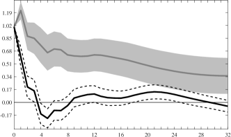
GDP
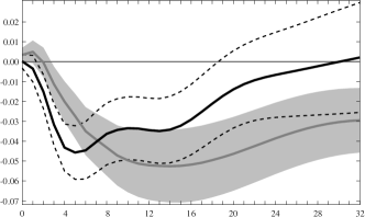
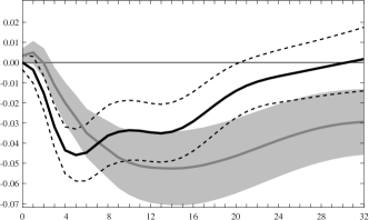
Consumption
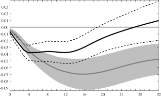
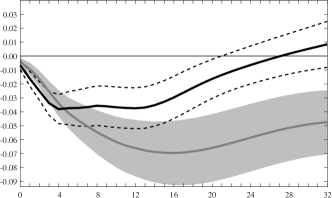
Fixed Investment

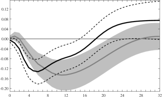
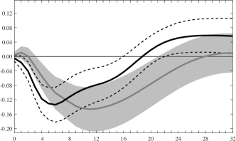
In each plot, the thick gray line is the IRF estimated by SW with a stationary DFM, while the shaded area is the 68% bootstrap confidence band. The thick black line is the IRF estimated with the non-stationary DFM, while the dotted line delimit the 68% bootstrap confidence band. The x-axis are quarters after the shocks, the y-axis are percentage points for all variables, but for Global Commodity Demand for the y-axis is standard deviations.

6.2 Application 2: the effect of news shocks

Starting with the seminal paper of Beaudry and Portier (2006), there has been a renewed interest in the idea that expectations about future fundamentals can be a driver of the business cycle. According to this theory, news about future productivity (a.k.a. news shocks) can generate a boom today and a bust in the future, if the realized productivity improvement is less than expected. In their paper, Beaudry and Portier (2006) by estimating a small size VECM find that a positive news shock has a positive impact on stock prices, output, consumption, investment, and hours worked. These results generated lots of interest because they are theoretically controversial. Indeed, in a neoclassical setting, in response to a positive news shock, hours worked should decrease—the wealth effect coming from higher stock prices induces households to consume more, and work less (i.e., desire more leisure)—and (at least initially) output and investment should decrease as well. In subsequent analyses, Barsky and Sims (2011), who use a small size SVAR in levels, overturn some of the results in Beaudry and Portier (2006). Specifically, they find that in response to a positive news shock, shock output and investment initially decline; after that, the response of output and investment tracks the path of Total Factor Productivity (TFP), rather than anticipate it. Furthermore, Barsky and Sims (2011) estimate a negative response of hours worked to a positive news shock.

Forni et al. (2014) (FGS hereafter) estimate the IRF to a news shock from a panel of 107 US quarterly macroeconomic time series, covering the period 1960:Q1 to 2010:Q4. In particular, they estimate a FAVAR with two observed factors (TFP and stock prices) and three latent factors extracted from principal components in levels, thus implicitly assuming all idiosyncratic components to be stationary. The news shock is identified by imposing that (i) it does not move TFP on impact, and (ii) it has maximal impact on TFP at the 60 quarters (15 years) horizon, see Section E in the complementary appendix for technical details.

Using the same dataset and identification strategy as in FGS, we estimate the effects of a news shock using our IRFs estimator in a FAVAR setting, as discussed in Remark 10 in Section 3.3, see also Section F2 in the complementary appendix for technical details. There are two main differences between our approach and the one used by FGS. First, we estimate the factors from differenced data properly de-trended, as explained in Section 3.1. In this way, we avoid the risk of detecting spurious factors due to the possible presence of $I(1)$ idiosyncratic components and/or deterministic linear trends, see Onatski and Wang (2020). Second, in addition to the FAVAR, we also consider IRFs obtained from a FAVECM with four cointegration relations (as suggested by the criteria in Section 4), which also account for cointegration between TFP, stock prices, and the three common factors.

Figure 2: Impulse-Response Functions to a News Shock

Panel a: VECM
TFP	Stock prices	Hours
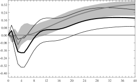
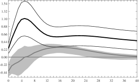
Consumption	Output	Investment
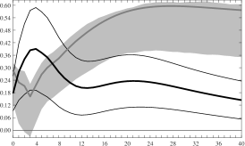
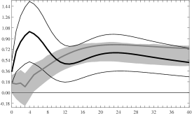
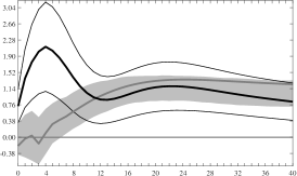
Panel b: VAR
TFP	Stock prices	Hours
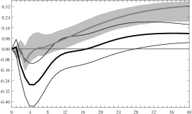
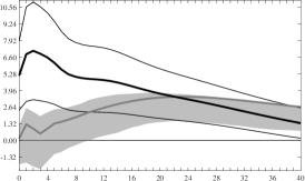
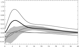
Consumption	Output	Investment

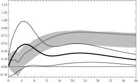
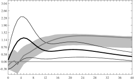
In each plot, the thick gray line is the IRF estimated by FGS, while the shaded area is the 68% bootstrap confidence band. The thick black line is the IRF estimated with our model, while the dotted line delimit the 68% bootstrap confidence band. The x-axis are quarters after the shocks, the y-axis are percentage points.

Figure 2 compares the IRFs to a news shock estimated by FGS (gray lines), with those estimated with our method (black lines), either estimating a FAVECM (Panel A) or a FAVAR in levels (Panel B) for the factors. Three main differences emerge. First, we estimate that hours worked respond positively to a news shock. Second, we estimate that investment and GDP increase on impact together with consumption, and their response leads the response of TFP. Third, as we can see from the hump-shaped response of consumption investment and output, our model predicts that in response to a positive news shock the economy first experiences a significant temporary boom, and then a temporary milder recession. In other words, our results are more in line with those of Beaudry and Portier (2006) and partly overturn those in Barsky and Sims (2011) and Forni et al. (2014).

A comment related only to our methodology is also in order: as we can see by comparing Panel (A) and Panel (B) in Figure 2, there are some differences between the IRFs estimated by fitting a FAVECM or a FAVAR. These differences emerge since the news shock is identified by imposing a restriction at 60 quarters horizon, and, as we discussed in Section 3.3, the long-run IRFs estimated with a VAR in levels are not consistently estimated in the long run. Therefore, we recommend for this application to use the FAVECM approach.

7 Conclusions

In this paper, we introduce a non-stationary Dynamic Factor Model (DFM) for large datasets, and we propose an estimator for the impulse response functions (IRFs). The natural use of this class of models in a macroeconomic context motivates the main assumptions upon which the present theory is built.

Estimation of IRFs is obtained with a two-step estimator based on principal components, and on a VECM—or an unrestricted VAR in levels—for the latent $I$(1) common factors. We prove consistency of the IRFs estimator when both the cross-sectional dimension $n$ and the sample size $T$ of the dataset grow to infinity. Furthermore, we also propose an information criterion to determine the number of common permanent shocks in a large dimensional setting.

A numerical study shows the validity and usefulness of our approach. Results show that if the short run is the focus, both the VECM and the unrestricted VAR in levels perform equally well, while if the long run is the focus, the VECM must be preferred.

In two empirical applications, we find that: (i) oil price shocks have just a temporary effect on US real activity; and, (ii) in response to a positive news shock, the economy first experiences a significant boom, and then a milder recession. Our results partly overturn those obtained by Stock and Watson (2016) and Forni et al. (2014), respectively, and show the importance of correctly accounting for the presence of cointegration in the common factors when estimating the IRFs.

In conclusion, compared to the stationary model commonly used in the literature, the non-stationary model proposed in this paper, which accounts for cointegration in the common factors, a feature that both economic and econometric theory suggest to be extremely likely, offers a more realistic representation of the data. Moreover, our approach has the advantage that it does not require to transform the variables to stationarity. Our empirical analysis shows that when estimating IRFs, cointegration matters, hence data should not be transformed. However, we have not investigated whether it matters when the goal is not estimating IRFs—for example, McCracken and Ng (2020) show that the cost of over differencing the data when forecasting is negligible. This is an empirical question and is part of our future research.

Appendix A Technical appendix

Norms

For any $m\times p$ matrix $\mathbf{B}$ with generic element $b_{ij}$, we denote its spectral norm as $\|\mathbf{B}\|=(\mu_{1}^{\mathbf{B}^{\prime}\mathbf{B}})^{1/2}$, where $\mu_{1}^{\mathbf{B}^{\prime}\mathbf{B}}$ is the largest eigenvalue of $\mathbf{B}^{\prime}\mathbf{B}$, the Frobenius norm as $\|\mathbf{B}\|_{F}=(\mbox{tr}(\mathbf{B}^{\prime}\mathbf{B}))^{1/2}=(\sum_{i}\sum_{j}b_{ij}^{2})^{1/2}$, and the column and row norm as $\|\mathbf{B}\|_{1}=\max_{j}\sum_{i}|b_{ij}|$ and $\|\mathbf{B}\|_{\infty}=\max_{i}\sum_{j}|b_{ij}|$, respectively. Throughout we also make use of Weyl’s inequality, for two $n\times n$ symmetric matrices $\mathbf{A}$ and $\mathbf{B}$, with eigenvalues $\mu_{j}^{A}$ and $\mu_{j}^{B}$:

$$|\mu_{j}^{A}-\mu_{j}^{B}|\leq\|\mathbf{A}-\mathbf{B}\|,\qquad j=1,\ldots,n.$$ (A1)

A.1 Proof of Proposition 1

First let us introduce some useful notation. Throughout define $\check{\mathbf{F}}_{t}=\mathbf{J}\mathbf{F}_{t}$ and $\check{\bm{\beta}}=\mathbf{J}\bm{\beta}$, where $\mathbf{J}$ is an $r\times r$ diagonal matrix with entries $\pm 1$ defined in Lemma 1, and note that $\check{\bm{\beta}}^{\prime}\check{\mathbf{F}}_{t}=\bm{\beta}^{\prime}{\mathbf{F}}_{t}$. Thus $\check{\bm{\beta}}$ is the matrix of cointegration vectors of $\check{\mathbf{F}}_{t}$ and we denote its orthogonal complement as $\check{\bm{\beta}}_{\perp}$, such that $\check{\bm{\beta}}_{\perp}^{\prime}\check{\bm{\beta}}=\mathbf{0}_{r-c\times c}$. Define the matrices

$$\widehat{\mathbf{M}}_{00}=\frac{1}{T}\sum_{t=1}^{T}\Delta\widehat{\mathbf{F}}_{t}\Delta\widehat{\mathbf{F}}_{t}^{\prime},\quad\widehat{\mathbf{M}}_{01}=\frac{1}{T}\sum_{t=1}^{T}\Delta\widehat{\mathbf{F}}_{t}\widehat{\mathbf{F}}_{t-1}^{\prime},\quad\widehat{\mathbf{M}}_{02}=\frac{1}{T}\sum_{t=1}^{T}\Delta\widehat{\mathbf{F}}_{t}\Delta\widehat{\mathbf{F}}_{t-1}^{\prime},$$

$$\widehat{\mathbf{M}}_{11}=\frac{1}{T}\sum_{t=1}^{T}\widehat{\mathbf{F}}_{t}\widehat{\mathbf{F}}_{t}^{\prime},\quad\widehat{\mathbf{M}}_{21}=\frac{1}{T}\sum_{t=1}^{T}\Delta\widehat{\mathbf{F}}_{t-1}^{\prime}\widehat{\mathbf{F}}_{t-1},\quad\widehat{\mathbf{M}}_{22}=\frac{1}{T}\sum_{t=1}^{T}\Delta\widehat{\mathbf{F}}_{t-1}\Delta\widehat{\mathbf{F}}_{t-1}^{\prime},$$

$$\widehat{\mathbf{S}}_{00}=\widehat{\mathbf{M}}_{00}-\widehat{\mathbf{M}}_{02}\widehat{\mathbf{M}}_{22}^{-1}\widehat{\mathbf{M}}_{20},\;\;\;\widehat{\mathbf{S}}_{01}=\widehat{\mathbf{M}}_{01}-\widehat{\mathbf{M}}_{02}\widehat{\mathbf{M}}_{22}^{-1}\widehat{\mathbf{M}}_{21},\;\;\;\widehat{\mathbf{S}}_{11}=\widehat{\mathbf{M}}_{11}-\widehat{\mathbf{M}}_{12}\widehat{\mathbf{M}}_{22}^{-1}\widehat{\mathbf{M}}_{21},$$

and denote by $\mathbf{M}_{ij}$ and $\mathbf{S}_{ij}$, for $i,j=0,1,2$, the analogous ones but computed by using $\check{\mathbf{F}}_{t}$. Finally, define the conditional covariance matrices

$$\check{\bm{\Omega}}_{00}=\mathsf{E}[\Delta\check{\mathbf{F}}_{t}\Delta\check{\mathbf{F}}_{t}^{\prime}|\Delta\check{\mathbf{F}}_{t-1}],\;\;\check{\bm{\Omega}}_{\check{\beta}\check{\beta}}=\mathsf{E}[\check{\bm{\beta}}^{\prime}\check{\mathbf{F}}_{t-1}\check{\mathbf{F}}_{t-1}^{\prime}\check{\bm{\beta}}|\Delta\check{\mathbf{F}}_{t-1}],\;\;\check{\bm{\Omega}}_{0\check{\beta}}=\mathsf{E}[\Delta\check{\mathbf{F}}_{t}\check{\mathbf{F}}_{t-1}^{\prime}\check{\bm{\beta}}|\Delta\check{\mathbf{F}}_{t-1}],\;\;\check{\bm{\Omega}}_{\check{\beta}0}=\check{\bm{\Omega}}_{0\check{\beta}}^{\prime}.$$

Let us start from part (i). Notice that if we denote the residuals of the regression of $\Delta\widehat{\mathbf{F}}_{t}$ and of $\widehat{\mathbf{F}}_{t-1}$ on $\Delta\widehat{\mathbf{F}}_{t-1}$ as $\widehat{\mathbf{e}}_{0t}$ and $\widehat{\mathbf{e}}_{1t}$, respectively then $\widehat{\mathbf{S}}_{ij}=T^{-1}\sum_{t=1}^{T}\widehat{\mathbf{e}}_{it}\widehat{\mathbf{e}}_{jt}^{\prime}$, with $i,j=0,1$. Consider the generalized eigenvalues problem

$$\det\big{(}\widehat{\mu}_{j}\widehat{\mathbf{S}}_{11}-\widehat{\mathbf{S}}_{10}\widehat{\mathbf{S}}_{00}^{-1}\widehat{\mathbf{S}}_{01}\big{)}=0,\quad j=1,\ldots,r.$$ (A2)

If $\widehat{\mathbf{U}}$ are the normalized eigenvectors of $\widehat{\mathbf{S}}_{11}^{-1/2}\widehat{\mathbf{S}}_{10}\widehat{\mathbf{S}}_{00}^{-1}\widehat{\mathbf{S}}_{01}\widehat{\mathbf{S}}_{11}^{-1/2}$, then $\widehat{\mathbf{P}}=\widehat{\mathbf{S}}_{11}^{-1/2}\widehat{\mathbf{U}}$ are eigenvectors of $\widehat{\mathbf{S}}_{11}-\widehat{\mathbf{S}}_{10}\widehat{\mathbf{S}}_{00}^{-1}\widehat{\mathbf{S}}_{01}$ with eigenvalues $\widehat{\mu}_{j}$. Then, the estimator $\widehat{\bm{\beta}}$ proposed by Johansen (1995) is given by the $c$ columns of $\widehat{\mathbf{P}}$ corresponding to the $c$ largest eigenvalues.

Analogously define $\widehat{\mathbf{U}}^{0}$ as the normalized eigenvectors of ${\mathbf{S}}_{11}^{-1/2}{\mathbf{S}}_{10}{\mathbf{S}}_{00}^{-1}{\mathbf{S}}_{01}{\mathbf{S}}_{11}^{-1/2}$ and define $\widehat{\mathbf{P}}^{0}={\mathbf{S}}_{11}^{-1/2}\widehat{\mathbf{U}}^{0}$. Then the estimator $\widehat{\bm{\beta}}^{0}$ that we would obtain if estimating a VECM on $\check{\mathbf{F}}_{t}$, is the matrix of the $c$ columns of $\widehat{\mathbf{P}}^{0}$, corresponding to the $c$ largest eigenvalues $\widehat{\mu}_{j}^{0}$ of ${\mathbf{S}}_{11}-{\mathbf{S}}_{10}{\mathbf{S}}_{00}^{-1}{\mathbf{S}}_{01}$, and such that

$$\det\big{(}\widehat{\mu}_{j}^{0}\mathbf{S}_{11}-\mathbf{S}_{10}\mathbf{S}_{00}^{-1}\mathbf{S}_{01}\big{)}=0,\quad j=1,\ldots,r.$$ (A3)

Notice that by definition the two estimators $\widehat{\bm{\beta}}$ and $\widehat{\bm{\beta}}^{0}$ are normalized in such a way that $\widehat{\bm{\beta}}^{\prime}\widehat{\mathbf{S}}_{11}\widehat{\bm{\beta}}=\mathbf{I}_{c}$ and $\widehat{\bm{\beta}}^{0^{\prime}}{\mathbf{S}}_{11}\widehat{\bm{\beta}}^{0}=\mathbf{I}_{c}$.

Consider then the $r\times r$ matrix $\mathbf{A}_{T}=\big{(}\check{\bm{\beta}}\;\;(T^{-1/2}{\check{\bm{\beta}}_{\perp*}})\big{)},$ where $\check{\bm{\beta}}_{\perp*}=\check{\bm{\beta}}_{\perp}(\check{\bm{\beta}}_{\perp}^{\prime}\check{\bm{\beta}}_{\perp})^{-1}$, and consider the equations

$$\det\big{[}\mathbf{A}_{T}^{\prime}\big{(}\widehat{\mu}_{j}\widehat{\mathbf{S}}_{11}-\widehat{\mathbf{S}}_{10}\widehat{\mathbf{S}}_{00}^{-1}\widehat{\mathbf{S}}_{01}\big{)}\mathbf{A}_{T}\big{]}=0,\quad j=1,\ldots,r,$$ (A4)

$$\det\big{[}\mathbf{A}_{T}^{\prime}\big{(}\widehat{\mu}_{j}^{0}\mathbf{S}_{11}-\mathbf{S}_{10}\mathbf{S}_{00}^{-1}\mathbf{S}_{01}\big{)}\mathbf{A}_{T}\big{]}=0,\quad j=1,\ldots,r.$$ (A5)

Clearly (A4) has the same solutions as (A2), but its eigenvectors are now given by $\mathbf{A}_{T}^{-1}\widehat{\mathbf{P}}$ and those corresponding to the largest $c$ eigenvalues are $\mathbf{A}_{T}^{-1}\widehat{\bm{\beta}}$. Analogously for (A5) we have the eigenvectors $\mathbf{A}_{T}^{-1}\widehat{\mathbf{P}}^{0}$ and the $c$ largest are given by $\mathbf{A}_{T}^{-1}\widehat{\bm{\beta}}^{0}$. Moreover,

$$\mathbf{A}_{T}^{\prime}\big{(}\widehat{\mathbf{S}}_{11}-\widehat{\mathbf{S}}_{10}\widehat{\mathbf{S}}_{00}^{-1}\widehat{\mathbf{S}}_{01}\big{)}\mathbf{A}_{T}-\mathbf{A}_{T}^{\prime}\big{(}{\mathbf{S}}_{11}-{\mathbf{S}}_{10}{\mathbf{S}}_{00}^{-1}{\mathbf{S}}_{01}\big{)}\mathbf{A}_{T}=$$

$$= \left\{\left[\begin{array}[]{cc}\check{\bm{\beta}}^{\prime}\widehat{\mathbf{S}}_{11}\check{\bm{\beta}}&T^{-1/2}\check{\bm{\beta}}^{\prime}\widehat{\mathbf{S}}_{11}\check{\bm{\beta}}_{\perp*}\\ T^{-1/2}\check{\bm{\beta}}_{\perp*}^{\prime}\widehat{\mathbf{S}}_{11}\check{\bm{\beta}}&T^{-1}\check{\bm{\beta}}_{\perp*}^{\prime}\widehat{\mathbf{S}}_{11}\check{\bm{\beta}}_{\perp*}\end{array}\right]-\left[\begin{array}[]{cc}\check{\bm{\beta}}^{\prime}{\mathbf{S}}_{11}\check{\bm{\beta}}&T^{-1/2}\check{\bm{\beta}}^{\prime}{\mathbf{S}}_{11}\check{\bm{\beta}}_{\perp*}\\ T^{-1/2}\check{\bm{\beta}}_{\perp*}^{\prime}{\mathbf{S}}_{11}\check{\bm{\beta}}&T^{-1}\check{\bm{\beta}}_{\perp*}^{\prime}{\mathbf{S}}_{11}\check{\bm{\beta}}_{\perp*}\end{array}\right]\right\}$$ (A10)

$$-\left\{\left[\begin{array}[]{cc}\check{\bm{\beta}}^{\prime}\widehat{\mathbf{S}}_{10}\widehat{\mathbf{S}}_{00}^{-1}\widehat{\mathbf{S}}_{01}\check{\bm{\beta}}&T^{-1/2}\check{\bm{\beta}}^{\prime}\widehat{\mathbf{S}}_{10}\widehat{\mathbf{S}}_{00}^{-1}\widehat{\mathbf{S}}_{01}\check{\bm{\beta}}_{\perp*}\\ T^{-1/2}\check{\bm{\beta}}_{\perp*}^{\prime}\widehat{\mathbf{S}}_{10}\widehat{\mathbf{S}}_{00}^{-1}\widehat{\mathbf{S}}_{01}\check{\bm{\beta}}&T^{-1}\check{\bm{\beta}}_{\perp*}^{\prime}\widehat{\mathbf{S}}_{10}\widehat{\mathbf{S}}_{00}^{-1}\widehat{\mathbf{S}}_{01}\check{\bm{\beta}}_{\perp*}\end{array}\right]\right.$$ (A13)

$$\left.\;\;\;-\left[\begin{array}[]{cc}\check{\bm{\beta}}^{\prime}{\mathbf{S}}_{10}{\mathbf{S}}_{00}^{-1}{\mathbf{S}}_{01}\check{\bm{\beta}}&T^{-1/2}\check{\bm{\beta}}^{\prime}{\mathbf{S}}_{10}{\mathbf{S}}_{00}^{-1}{\mathbf{S}}_{01}\check{\bm{\beta}}_{\perp*}\\ T^{-1/2}\check{\bm{\beta}}_{\perp*}^{\prime}{\mathbf{S}}_{10}{\mathbf{S}}_{00}^{-1}{\mathbf{S}}_{01}\check{\bm{\beta}}&T^{-1}\check{\bm{\beta}}_{\perp*}^{\prime}{\mathbf{S}}_{10}{\mathbf{S}}_{00}^{-1}{\mathbf{S}}_{01}\check{\bm{\beta}}_{\perp*}\end{array}\right]\right\}=O_{p}(\vartheta_{nT,\delta,\eta}).$$ (A16)

This result is proved by using Lemma D11(ii), D11(iii) and D11(vi) for the first term on the rhs, and by using Lemma D11(i), D11(iv) and D11(v) for the second term. Thus, from (A16), for any $j=1,\ldots,r$, from Weyl’s inequality (C3), we have

$$\big{|}\widehat{\mu}_{j}-\widehat{\mu}_{j}^{0}\big{|}\leq\big{\|}\mathbf{A}_{T}^{\prime}\big{(}\widehat{\mathbf{S}}_{11}-\widehat{\mathbf{S}}_{10}\widehat{\mathbf{S}}_{00}^{-1}\widehat{\mathbf{S}}_{01}\big{)}\mathbf{A}_{T}-\mathbf{A}_{T}^{\prime}\big{(}{\mathbf{S}}_{11}-{\mathbf{S}}_{10}{\mathbf{S}}_{00}^{-1}{\mathbf{S}}_{01}\big{)}\mathbf{A}_{T}\big{\|}=O_{p}(\vartheta_{nT,\delta,\eta}).$$ (A17)

Then, because of Lemmas D6(ii) and D12, and from (A16), (A17), and Slutsky’s theorem, as $n,T\to\infty$, we have (see also Lemma 13.1 in Johansen, 1995)

$$\det \bigg{[}\mathbf{A}_{T}^{\prime}\Big{(}\widehat{\mu}_{j}\widehat{\mathbf{S}}_{11}-\widehat{\mathbf{S}}_{10}\widehat{\mathbf{S}}_{00}^{-1}\widehat{\mathbf{S}}_{01}\Big{)}\mathbf{A}_{T}\bigg{]}=\det\bigg{[}\mathbf{A}_{T}^{\prime}\Big{(}\widehat{\mu}^{0}_{j}{\mathbf{S}}_{11}-{\mathbf{S}}_{10}{\mathbf{S}}_{00}^{-1}{\mathbf{S}}_{01}\Big{)}\mathbf{A}_{T}\bigg{]}+O_{p}(\vartheta_{nT,\delta,\eta})$$ (A18)

$$\stackrel{{\scriptstyle d}}{{\to}} \det\bigg{(}\widehat{\mu}^{0}_{j}\check{\bm{\Omega}}_{\check{\beta}\check{\beta}}-\check{\bm{\Omega}}_{\check{\beta}0}\check{\bm{\Omega}}_{00}^{-1}\check{\bm{\Omega}}_{0\check{\beta}}\bigg{)}\;\det\bigg{[}\widehat{\mu}^{0}_{j}\check{\bm{\beta}}_{\perp*}^{\prime}\mathbf{C}(1)\bigg{(}\int_{0}^{1}\mathbf{W}_{q}(\tau)\mathbf{W}_{q}^{\prime}(\tau)\mbox{d}\tau\bigg{)}\mathbf{C}^{\prime}(1)\check{\bm{\beta}}_{\perp*}\bigg{]}.$$

where $\mathbf{W}_{q}(\cdot)$ is a $q$-dimensional Brownian motion with covariance $\mathbf{I}_{q}$. The first term on the rhs of (A18) has only $c$ solutions different from zero (the matrix is positive definite) while the remaining $r-c$ solutions come from the second term and are all zero since ${\rm rk}(\mathbf{C}(1))=r-c=q-d$. Therefore, as $n,T\to\infty$ both $\mathbf{A}_{T}^{-1}\widehat{\mathbf{P}}$ and $\mathbf{A}_{T}^{-1}\widehat{\mathbf{P}}^{0}$ span a space of dimension $c$ given by their first $c$ eigenvectors, which by definition are given by $\mathbf{A}_{T}^{-1}\widehat{\bm{\beta}}$ and $\mathbf{A}_{T}^{-1}\widehat{\bm{\beta}}^{0}$, respectively. As a consequence, there exist a positive real $D_{1}$ such that $\widehat{\mu}_{j}^{0}>D_{1}$ for $j=1,\ldots,c$. From (A16) and Theorem 2 in Yu et al. (2015), there exists an orthogonal $c\times c$ matrix $\mathbf{O}_{c}$ such that

$$\big{\|}\mathbf{A}_{T}^{-1} \widehat{\bm{\beta}}\mathbf{O}_{c}-\mathbf{A}_{T}^{-1}\widehat{\bm{\beta}}^{0}\big{\|}\leq\frac{2^{3/2}\sqrt{c}\big{\|}\mathbf{A}_{T}^{\prime}\big{(}\widehat{\mathbf{S}}_{11}-\widehat{\mathbf{S}}_{10}\widehat{\mathbf{S}}_{00}^{-1}\widehat{\mathbf{S}}_{01}\big{)}\mathbf{A}_{T}-\mathbf{A}_{T}^{\prime}\big{(}{\mathbf{S}}_{11}-{\mathbf{S}}_{10}{\mathbf{S}}_{00}^{-1}{\mathbf{S}}_{01}\big{)}\mathbf{A}_{T}\big{\|}}{\widehat{\mu}_{c}^{0}}$$

$$\leq\frac{2^{3/2}\sqrt{c}\big{\|}\mathbf{A}_{T}^{\prime}\big{(}\widehat{\mathbf{S}}_{11}-\widehat{\mathbf{S}}_{10}\widehat{\mathbf{S}}_{00}^{-1}\widehat{\mathbf{S}}_{01}\big{)}\mathbf{A}_{T}-\mathbf{A}_{T}^{\prime}\big{(}{\mathbf{S}}_{11}-{\mathbf{S}}_{10}{\mathbf{S}}_{00}^{-1}{\mathbf{S}}_{01}\big{)}\mathbf{A}_{T}\big{\|}}{D_{1}}=O_{p}(\vartheta_{nT,\delta,\eta}).$$ (A19)

Define the transformed estimators

$$\widetilde{\bm{\beta}}=\widehat{\bm{\beta}}\mathbf{O}_{c}(\check{\bm{\beta}}_{*}^{\prime}\widehat{\bm{\beta}}\mathbf{O}_{c})^{-1},\qquad\widetilde{\bm{\beta}}^{0}=\widehat{\bm{\beta}}^{0}(\check{\bm{\beta}}_{*}^{\prime}\widehat{\bm{\beta}}^{0})^{-1}.$$ (A20)

From Lemma 13.1 in Johansen (1995), we have (recall that $\check{\bm{\beta}}^{\prime}_{\perp}\check{\bm{\beta}}=\mathbf{0}_{r-c\times c}$)

$$\mathbf{A}_{T}^{-1}\widetilde{\bm{\beta}}^{0}=\mathbf{A}_{T}^{-1}\big{(}\check{\bm{\beta}}+\check{\bm{\beta}}_{\perp*}\check{\bm{\beta}}_{\perp}^{\prime}\widetilde{\bm{\beta}}^{0}\big{)}=\left(\begin{array}[]{c}\mathbf{I}_{c}\\ \sqrt{T}\check{\bm{\beta}}^{\prime}_{\perp}\widetilde{\bm{\beta}}^{0}\end{array}\right)=\left(\begin{array}[]{c}\mathbf{I}_{c}\\ \sqrt{T}\check{\bm{\beta}}^{\prime}_{\perp}(\widetilde{\bm{\beta}}^{0}-\check{\bm{\beta}})\end{array}\right)=\left(\begin{array}[]{c}\mathbf{I}_{c}\\ o_{p}(1)\end{array}\right),$$ (A21)

since $\mathbf{A}_{T}^{-1}\widetilde{\bm{\beta}}^{0}$ spans a space of dimension $c$. In the same way, we have

$$\mathbf{A}_{T}^{-1}\widetilde{\bm{\beta}}=\left(\begin{array}[]{c}\mathbf{I}_{c}\\ \sqrt{T}\check{\bm{\beta}}^{\prime}_{\perp}\widetilde{\bm{\beta}}\end{array}\right)=\left(\begin{array}[]{c}\mathbf{I}_{c}\\ \sqrt{T}\check{\bm{\beta}}^{\prime}_{\perp}(\widetilde{\bm{\beta}}-\check{\bm{\beta}})\end{array}\right)=\left(\begin{array}[]{c}\mathbf{I}_{c}\\ \sqrt{T}\check{\bm{\beta}}^{\prime}_{\perp}(\widetilde{\bm{\beta}}^{0}-\check{\bm{\beta}})+\sqrt{T}\check{\bm{\beta}}^{\prime}_{\perp}(\widetilde{\bm{\beta}}-\widetilde{\bm{\beta}}_{0})\end{array}\right).$$ (A22)

Now since $\mbox{span}(\mathbf{A}_{T}^{-1}\widetilde{\bm{\beta}})=\mbox{span}(\mathbf{A}_{T}^{-1}\widehat{\bm{\beta}})$, also (A22) spans a space of dimension $c$. Then, since also $\mbox{span}(\mathbf{A}_{T}^{-1}\widetilde{\bm{\beta}}^{0})=\mbox{span}(\mathbf{A}_{T}^{-1}\widehat{\bm{\beta}}^{0})$, by comparing (A21) and (A22), and using (A.1) and (A20), we have

$$\big{\|}\sqrt{T}\check{\bm{\beta}}^{\prime}_{\perp}(\widetilde{\bm{\beta}}-\widetilde{\bm{\beta}}_{0})\big{\|}=\big{\|}\mathbf{A}_{T}^{-1}\widetilde{\bm{\beta}}-\mathbf{A}_{T}^{-1}\widetilde{\bm{\beta}}^{0}\big{\|}=O_{p}(\vartheta_{nT,\delta,\eta}).$$ (A23)

Therefore, given that $\|\check{\bm{\beta}}^{\prime}_{\perp}\|=O(1)$, from (A21) and (A23), we have

$$\big{\|}\widetilde{\bm{\beta}}-\check{\bm{\beta}}\big{\|}\leq\big{\|}\widetilde{\bm{\beta}}^{0}-\check{\bm{\beta}}\big{\|}+\big{\|}\widetilde{\bm{\beta}}^{0}-\widetilde{\bm{\beta}}\big{\|}=o_{p}\left(\frac{1}{\sqrt{T}}\right)+O_{p}\left(\frac{\vartheta_{nT,\delta,\eta}}{\sqrt{T}}\right).$$ (A24)

Finally, from (A20), we can always define a $c\times c$ orthogonal matrix $\mathbf{Q}$, which depends on $\mathbf{O}_{c}$, and such that $\widetilde{\bm{\beta}}\mathbf{Q}=\widehat{\bm{\beta}}$ (see also pp.179-180 in Johansen, 1995, for a discussion about the choice of the identification matrix $\mathbf{Q}$). Therefore, we have

$$\big{\|}\widehat{\bm{\beta}}-\check{\bm{\beta}}\mathbf{Q}\big{\|}=\big{\|}\widehat{\bm{\beta}}-\mathbf{J}{\bm{\beta}}\mathbf{Q}\big{\|}=O_{p}\left(\frac{\vartheta_{nT,\delta,\eta}}{\sqrt{T}}\right),$$

which completes the proof of part (i).

Once we have $\widehat{\bm{\beta}}$, the other parameters are estimated by linear regression as

$$\widehat{\bm{\alpha}}=\widehat{\mathbf{S}}_{01}\widehat{\bm{\beta}}\big{(}\widehat{\bm{\beta}}^{\prime}\widehat{\mathbf{S}}_{11}\widehat{\bm{\beta}}\big{)}^{-1},\qquad\widehat{\mathbf{G}}_{1}=\big{(}\widehat{\mathbf{M}}_{02}-\widehat{\bm{\alpha}}\widehat{\bm{\beta}}^{\prime}\widehat{\mathbf{M}}_{12}\big{)}\widehat{\mathbf{M}}_{22}^{-1}.$$ (A25)

For part (ii), first notice that, by definition from a VECM for $\mathbf{F}_{t}$, since $\mathbf{u}_{t}$ is independent because of Assumption 1(a), we have $\bm{\alpha}=\mathsf{E}[\Delta\mathbf{F}_{t}\mathbf{F}_{t-1}^{\prime}\bm{\beta}|\Delta\mathbf{F}_{t-1}]\big{(}\mathsf{E}[\bm{\beta}^{\prime}\mathbf{F}_{t}\mathbf{F}_{t-1}^{\prime}\bm{\beta}|\Delta\mathbf{F}_{t-1}]\big{)}^{-1}.$ Therefore, since conditioning on $\Delta\mathbf{F}_{t-1}$ is equivalent to conditioning on $\mathbf{J}\Delta\mathbf{F}_{t-1}=\Delta\check{\mathbf{F}}_{t-1}$ and since $\bm{\beta}^{\prime}\mathbf{F}_{t}=\check{\bm{\beta}}^{\prime}\check{\mathbf{F}}_{t}$, we immediately have

$$\check{\bm{\alpha}}=\mathbf{J}\bm{\alpha}= \mathbf{J}\mathsf{E}[\Delta\mathbf{F}_{t}\check{\mathbf{F}}_{t-1}^{\prime}\check{\bm{\beta}}|\Delta\check{\mathbf{F}}_{t-1}]\big{(}\mathsf{E}[\check{\bm{\beta}}^{\prime}\check{\mathbf{F}}_{t}\check{\mathbf{F}}_{t-1}^{\prime}\check{\bm{\beta}}|\Delta\check{\mathbf{F}}_{t-1}]\big{)}^{-1}$$

$$= \mathsf{E}[\Delta\check{\mathbf{F}}_{t}\check{\mathbf{F}}_{t-1}^{\prime}\check{\bm{\beta}}|\Delta\check{\mathbf{F}}_{t-1}]\big{(}\mathsf{E}[\check{\bm{\beta}}^{\prime}\check{\mathbf{F}}_{t}\check{\mathbf{F}}_{t-1}^{\prime}\check{\bm{\beta}}|\Delta\check{\mathbf{F}}_{t-1}]\big{)}^{-1}=\check{\bm{\Omega}}_{0\check{\beta}}\check{\bm{\Omega}}_{\check{\beta}\check{\beta}}^{-1}.$$

Then,

$$\big{\|}\widehat{\mathbf{S}}_{01}\widehat{\bm{\beta}}-\check{\bm{\Omega}}_{0\check{\beta}}\mathbf{Q}\big{\|}\leq \big{\|}\widehat{\mathbf{S}}_{01}(\widehat{\bm{\beta}}-\check{\bm{\beta}}\mathbf{Q})\big{\|}+\big{\|}\widehat{\mathbf{S}}_{01}\check{\bm{\beta}}\mathbf{Q}-\mathbf{S}_{01}\check{\bm{\beta}}\mathbf{Q}\big{\|}+\big{\|}\mathbf{S}_{01}\check{\bm{\beta}}\mathbf{Q}-\check{\bm{\Omega}}_{0\check{\beta}}\mathbf{Q}\big{\|}=O_{p}(\vartheta_{nT,\delta,\eta}),$$ (A26)

using part (i) and the fact that $\|\widehat{\mathbf{S}}_{01}\|=O_{p}(T^{1/2})$ for the first term on the rhs, Lemma D11(iv) for the second term, and Lemma D12(iii) for the third term. Analogously we have

$$\big{\|}\widehat{\bm{\beta}}^{\prime}\widehat{\mathbf{S}}_{11}\widehat{\bm{\beta}}-\mathbf{Q}^{\prime}\check{\bm{\Omega}}_{\check{\beta}\check{\beta}}\mathbf{Q}\big{\|}\leq \big{\|}(\widehat{\bm{\beta}}^{\prime}-\mathbf{Q}^{\prime}\check{\bm{\beta}}^{\prime})\widehat{\mathbf{S}}_{11}(\widehat{\bm{\beta}}-\check{\bm{\beta}}\mathbf{Q})\big{\|}+\big{\|}\mathbf{Q}^{\prime}\check{\bm{\beta}}^{\prime}\widehat{\mathbf{S}}_{11}\check{\bm{\beta}}\mathbf{Q}-\mathbf{Q}^{\prime}\check{\bm{\beta}}^{\prime}\mathbf{S}_{11}\check{\bm{\beta}}\mathbf{Q}\big{\|}$$

$$+\big{\|}\mathbf{Q}^{\prime}\check{\bm{\beta}}^{\prime}\mathbf{S}_{11}\check{\bm{\beta}}\mathbf{Q}-\mathbf{Q}^{\prime}\check{\bm{\Omega}}_{\check{\beta}\check{\beta}}\mathbf{Q}\big{\|}=O_{p}(\vartheta_{nT,\delta,\eta}),$$ (A27)

using part (i) and the fact that $\|\widehat{\mathbf{S}}_{11}\|=O_{p}(T)$ for the first term, Lemma D11(ii) for the second term, and Lemma D12(ii) for the third term. Therefore, from (A25), (A26), and (A27), and since $\mathbf{Q}$ is orthogonal, we have

$$\big{\|}\widehat{\bm{\alpha}}-\check{\bm{\alpha}}\mathbf{Q}\big{\|}=\big{\|}\widehat{\bm{\alpha}}-\mathbf{J}{\bm{\alpha}}\mathbf{Q}\big{\|}=O_{p}(\vartheta_{nT,\delta,\eta}),$$

which proves part (ii).

For part (iii), notice that, by definition, we have:

$$\check{\mathbf{G}}_{1}=\mathbf{H}\mathbf{G}_{1}\mathbf{H}^{\prime}=\big{(}\bm{\Gamma}_{1}^{\Delta\check{F}}-\check{\bm{\alpha}}\mathsf{E}[\check{\bm{\beta}}^{\prime}\check{\mathbf{F}}_{t-1}\Delta\check{\mathbf{F}}_{t-1}^{\prime}]\big{)}(\bm{\Gamma}_{0}^{\Delta\check{F}})^{-1}.$$ (A28)

Then, from (A25),

$$\big{\|}\widehat{\mathbf{G}}_{1}-\check{\mathbf{G}}_{1}\big{\|}\leq \big{\|}\big{(}\widehat{\mathbf{M}}_{02}-\widehat{\bm{\alpha}}\widehat{\bm{\beta}}^{\prime}\widehat{\mathbf{M}}_{12}\big{)}\widehat{\mathbf{M}}_{22}^{-1}-\big{(}\widehat{\mathbf{M}}_{02}-\check{\bm{\alpha}}\check{\bm{\beta}}^{\prime}\widehat{\mathbf{M}}_{12}\big{)}\widehat{\mathbf{M}}_{22}^{-1}\big{\|}$$

$$+\big{\|}\big{(}\widehat{\mathbf{M}}_{02}-\check{\bm{\alpha}}\check{\bm{\beta}}^{\prime}\widehat{\mathbf{M}}_{12}\big{)}\widehat{\mathbf{M}}_{22}^{-1}-\big{(}{\mathbf{M}}_{02}-\check{\bm{\alpha}}\check{\bm{\beta}}^{\prime}{\mathbf{M}}_{12}\big{)}{\mathbf{M}}_{22}^{-1}\big{\|}$$

$$+\big{\|}\big{(}{\mathbf{M}}_{02}-\check{\bm{\alpha}}\check{\bm{\beta}}^{\prime}{\mathbf{M}}_{12}\big{)}{\mathbf{M}}_{22}^{-1}-\big{(}\bm{\Gamma}_{1}^{\Delta\check{F}}-\check{\bm{\alpha}}\mathsf{E}[\check{\bm{\beta}}^{\prime}\check{\mathbf{F}}_{t-1}\Delta\check{\mathbf{F}}_{t-1}^{\prime}]\big{)}(\bm{\Gamma}_{0}^{\Delta\check{F}})^{-1}\big{\|}=O_{p}(\vartheta_{nT,\delta,\eta}),$$

since the first term on the rhs is $O_{p}(\vartheta_{nT,\delta,\eta})$ by parts (i) and (ii) and since $\check{\bm{\alpha}}\mathbf{Q}\mathbf{Q}^{\prime}\check{\bm{\beta}}^{\prime}=\check{\bm{\alpha}}\check{\bm{\beta}}^{\prime}$, the second term is $O_{p}(\vartheta_{nT,\delta,\eta})$ by Lemma D10(iii), D10(iv) and D10(vii), and the third term is $O_{p}(T^{-1/2})$ by Lemma D6(i) and D6(vi) and Chebychev’s inequality. This, together with (A28), proves part (iii).

For part (iv), first consider the VECM residuals $\widehat{\mathbf{w}}_{t}=\Delta\widehat{\mathbf{F}}_{t}-\widehat{\bm{\alpha}}\widehat{\bm{\beta}}^{\prime}\widehat{\mathbf{F}}_{t-1}-\widehat{\mathbf{G}}_{1}\Delta\widehat{\mathbf{F}}_{t-1}$ and notice that their sample covariance is also written as

$$\widehat{\bm{\Gamma}}_{0}^{w}= \frac{1}{T}\sum_{t=1}^{T}\widehat{\mathbf{w}}_{t}\widehat{\mathbf{w}}_{t}^{\prime}=\frac{1}{T}\sum_{t=1}^{T}(\Delta\widehat{\mathbf{F}}_{t}-\widehat{\bm{\alpha}}\widehat{\bm{\beta}}^{\prime}\widehat{\mathbf{F}}_{t-1}-\widehat{\mathbf{G}}_{1}\Delta\widehat{\mathbf{F}}_{t-1})(\Delta\widehat{\mathbf{F}}_{t}-\widehat{\bm{\alpha}}\widehat{\bm{\beta}}^{\prime}\widehat{\mathbf{F}}_{t-1}-\widehat{\mathbf{G}}_{1}\Delta\widehat{\mathbf{F}}_{t-1})^{\prime}$$

$$= \widehat{\mathbf{M}}_{00}+\widehat{\bm{\alpha}}\widehat{\bm{\beta}}^{\prime}\widehat{\mathbf{M}}_{11}\widehat{\bm{\beta}}\widehat{\bm{\alpha}}^{\prime}+\widehat{\mathbf{G}}_{1}\widehat{\mathbf{M}}_{22}\widehat{\mathbf{G}}_{1}^{\prime}-\widehat{\mathbf{M}}_{01}\widehat{\bm{\beta}}\widehat{\bm{\alpha}}^{\prime}-\widehat{\bm{\alpha}}\widehat{\bm{\beta}}^{\prime}\widehat{\mathbf{M}}_{12}\widehat{\mathbf{G}}_{1}^{\prime}-\widehat{\bm{\alpha}}\widehat{\bm{\beta}}^{\prime}\widehat{\mathbf{M}}_{10}-\widehat{\mathbf{G}}_{1}\widehat{\mathbf{M}}_{20}-\widehat{\mathbf{G}}_{1}\widehat{\mathbf{M}}_{21}\widehat{\bm{\beta}}\widehat{\bm{\alpha}}^{\prime}.$$

Then from parts (i), (ii) and (iii), Lemma D10(ii) through D10(vi) and D10(ix), and Lemma D6(i) and D6(vi), we can prove that

$$\big{\|}\widehat{\bm{\Gamma}}_{0}^{w}-\mathbf{J}{\bm{\Gamma}}_{0}^{w}\mathbf{J}\big{\|}=O_{p}(\vartheta_{nT,\delta,\eta}),$$ (A29)

where ${\bm{\Gamma}}_{0}^{w}=\mathsf{E}\big{[}\mathbf{w}_{t}\mathbf{w}_{t}^{\prime}\big{]}=\mathsf{E}\big{[}(\Delta{\mathbf{F}}_{t}-{\bm{\alpha}}{\bm{\beta}}^{\prime}{\mathbf{F}}_{t-1}-{\mathbf{G}}_{1}\Delta{\mathbf{F}}_{t-1})(\Delta{\mathbf{F}}_{t}-{\bm{\alpha}}{\bm{\beta}}^{\prime}{\mathbf{F}}_{t-1}-{\mathbf{G}}_{1}\Delta{\mathbf{F}}_{t-1})^{\prime}\big{]}$.

By (19), we have $\mathbf{w}_{t}=\mathbf{K}\mathbf{u}_{t}$, therefore, since the shocks $\mathbf{u}_{t}$ are orthonormal by Assumption 1(a), we have $\bm{\Gamma}_{0}^{w}=\mathbf{K}\mathbf{K}^{\prime}$. Denote as $\mu_{j}^{w}$, $j=1,\ldots,q$, the $q$ largest eigenvalues of $\bm{\Gamma}_{0}^{w}$, which are also the $q$ eigenvalues of $\mathbf{K}^{\prime}\mathbf{K}$ and are asymptotically distinct by the assumption made in the statement of Proposition 1. Then, since $\mathbf{K}=\mathbf{Q}(0)=\mathbf{C}(0)$, from Assumption 1 and the model given in (6), we have ${\rm rk}(\mathbf{K})=q$, and therefore there exist positive reals $\underline{D}_{j},\overline{D}_{j}$ and an integer $\bar{n}$, such that $\underline{D}_{j}>\overline{D}_{j+1}$ for $j=1,\ldots,q-1$, and $\underline{D}_{j}\leq\mu_{j}^{w}\leq\overline{D}_{j}$, for $n>\bar{n}$ and $j=1,\ldots,q$.

Denote as $\mu_{j}^{w}$ the eigenvalues of $\bm{\Gamma}_{0}^{w}$, which are also the eigenvalues of $\mathbf{K}^{\prime}\mathbf{K}$. Then, Denote by $\bm{w}_{j}^{w}$ the eigenvector corresponding to $\mu_{j}^{w}$ and define as $\mathbf{M}^{w}$ the $q\times q$ diagonal matrix with entries $\mu_{j}^{w}$ and as $\mathbf{W}^{w}=(\bm{w}_{1}^{w}\cdots\bm{w}_{q}^{w})$ the corresponding $r\times q$ matrix of normalized eigenvectors. For any $q\times q$ invertible matrix $\mathbf{P}$, we can always write $\mathbf{w}_{t}=\big{[}\mathbf{K}\mathbf{P}\big{]}\big{[}\mathbf{P}^{-1}\mathbf{u}_{t}\big{]}=\mathbf{H}\mathbf{v}_{t}$. In particular, let us choose $\mathbf{P}$ to be such that (recall the identity $\mathbf{w}_{t}=\mathbf{W}^{w}\mathbf{W}^{w^{\prime}}\mathbf{w}_{t}$)

$$\mathbf{v}_{t}=\mathbf{P}^{-1}\mathbf{u}_{t}=(\mathbf{M}^{w})^{-1/2}\mathbf{W}^{w^{\prime}}\mathbf{w}_{t},\qquad\mathbf{H}=\mathbf{K}\mathbf{P}=\mathbf{W}^{w}(\mathbf{M}^{w})^{1/2}.$$ (A30)

Then, for this choice of $\mathbf{P}$, we have $\bm{\Gamma}^{v}_{0}=\mathsf{E}[\mathbf{v}_{t}\mathbf{v}_{t}^{\prime}]=(\mathbf{P})^{-1}(\mathbf{P})^{-1^{\prime}}=\mathbf{I}_{q}$, and therefore $\mathbf{P}$ must be orthogonal, i.e., $\mathbf{P}^{-1}=\mathbf{P}^{\prime}$.

Now, consider the estimators: $\widehat{\mathbf{K}}=\widehat{\mathbf{W}}^{w}(\widehat{\mathbf{M}}^{w})^{1/2}$ and $\widehat{\mathbf{u}}_{t}=(\widehat{\mathbf{M}}^{w})^{-1/2}\widehat{\mathbf{W}}^{w^{\prime}}\widehat{\mathbf{w}}_{t}$, where $\widehat{\mathbf{W}}^{w}=(\widehat{\bm{w}}_{1}^{w}\cdots\widehat{\bm{w}}_{q}^{w})$ is the $r\times q$ matrix of the first $q$ normalized eigenvectors of $\widehat{\bm{\Gamma}}^{w}_{0}$ and $\widehat{\mathbf{M}}^{w}$ is the $q\times q$ diagonal matrix of the corresponding eigenvalues $\widehat{\mu}_{j}^{w}$. Then, since $\underline{D}_{j}>\overline{D}_{j+1}$ for $j=1,\ldots,q-1$, by Corollary 1 in Yu et al. (2015) and because of (A29), for $j=1,\ldots,q$, we have (note that $\mathbf{J}\mathbf{W}^{w}$ are eigenvectors of $\mathbf{J}\bm{\Gamma}_{0}^{w}\mathbf{J}$ with eigenvalues $\mu_{j}^{w}$)

$$\big{\|}\widehat{\bm{w}}_{j}^{w}-\mathbf{J}\bm{w}_{j}^{w}s_{j}^{w}\big{\|} \leq\frac{2^{3/2}\big{\|}\widehat{\bm{\Gamma}}_{0}^{w}-\mathbf{J}{\bm{\Gamma}}_{0}^{w}\mathbf{J}\big{\|}}{\min((\mu_{j-1}^{w}-\mu_{j}^{w}),(\mu_{j}^{w}-\mu_{j+1}^{w}))}\leq\frac{2^{3/2}\big{\|}\widehat{\bm{\Gamma}}_{0}^{w}-\mathbf{J}{\bm{\Gamma}}_{0}^{w}\mathbf{J}\big{\|}}{\min((\underline{D}_{j-1}-\overline{D}_{j}),(\underline{D}_{j}-\overline{D}_{j+1}))}=O_{p}(\vartheta_{nT,\delta,\eta}),$$ (A31)

where $s_{j}^{w}=\mbox{sign}(\widehat{\bm{w}}_{j}^{w^{\prime}}\mathbf{J}\bm{w}_{j}^{w})$ and we define $\mu_{0}^{w}=\infty$. Define as $\mathbf{J}^{w}$ the $q\times q$ diagonal matrix with entries $s_{j}^{w}$, then from (A31), we have

$$\big{\|}\widehat{\mathbf{W}}^{w}-\mathbf{J}\mathbf{W}^{w}\mathbf{J}^{w}\big{\|}\leq\sqrt{\sum_{j=1}^{q}\big{\|}\widehat{\bm{w}}_{j}^{w}-\mathbf{J}\bm{w}_{j}^{w}s_{j}^{w}\big{\|}^{2}}=O_{p}(\vartheta_{nT,\delta,\eta}).$$ (A32)

Now, let us consider the estimated eigenvalues. From, (A29) and using Weyl’s inequality (C3), we have

$$\big{|}\widehat{\mu}^{w}_{j}-{\mu}^{w}_{j}\big{|}\leq\big{\|}\widehat{\bm{\Gamma}}_{0}^{w}-\mathbf{J}{\bm{\Gamma}}_{0}^{w}\mathbf{J}\big{\|}=O_{p}(\vartheta_{nT,\delta,\eta}),\qquad j=1,\ldots,q,$$ (A33)

which implies

$$\big{|}(\widehat{\mu}^{w}_{j})^{1/2}-({\mu}^{w}_{j})^{1/2}\big{|}\leq\frac{\big{|}\widehat{\mu}^{w}_{j}-{\mu}^{w}_{j}\big{|}}{2({\mu}^{w}_{j})^{1/2}}\leq\frac{\big{|}\widehat{\mu}^{w}_{j}-{\mu}^{w}_{j}\big{|}}{2D^{1/2}}=O_{p}(\vartheta_{nT,\delta,\eta}),\qquad j=1,\ldots,q.$$ (A34)

Therefore, from (A34), we have

$$\|(\widehat{\mathbf{M}}^{w})^{1/2}-(\mathbf{M}^{w})^{1/2}\|\leq\sqrt{\sum_{j=1}^{q}\big{(}(\widehat{\mu}^{w}_{j})^{1/2}-({\mu}^{w}_{j})^{1/2}\big{)}^{2}}=O_{p}(\vartheta_{nT,\delta,\eta}),$$ (A35)

Let us define the orthogonal matrix $\mathbf{R}=\mathbf{J}^{w}\mathbf{P}^{\prime}$, then, using (A30), (A32), and (A35), we have (notice that $\mathbf{P}\mathbf{J}^{w}=\mathbf{P}(\mathbf{M}^{w})^{-1/2}\mathbf{J}^{w}(\mathbf{M}^{w})^{1/2}$ and $\mathbf{H}(\mathbf{M}^{w})^{-1/2}=\mathbf{W}^{w}$)

$$\big{\|}\widehat{\mathbf{K}}-\mathbf{J}\mathbf{K}\mathbf{R}^{\prime}\big{\|} =\big{\|}\widehat{\mathbf{W}}^{w}(\widehat{\mathbf{M}}^{w})^{1/2}-\mathbf{J}\mathbf{K}\mathbf{P}\mathbf{J}^{w}\big{\|}=\big{\|}\widehat{\mathbf{W}}^{w}(\widehat{\mathbf{M}}^{w})^{1/2}-\mathbf{J}\mathbf{K}\mathbf{P}(\mathbf{M}^{w})^{-1/2}\mathbf{J}^{w}(\mathbf{M}^{w})^{1/2}\big{\|}$$

$$=\big{\|}\widehat{\mathbf{W}}^{w}(\widehat{\mathbf{M}}^{w})^{1/2}-\mathbf{J}\mathbf{H}(\mathbf{M}^{w})^{-1/2}\mathbf{J}^{w}(\mathbf{M}^{w})^{1/2}\big{\|}=\big{\|}\widehat{\mathbf{W}}^{w}(\widehat{\mathbf{M}}^{w})^{1/2}-\mathbf{J}\mathbf{W}^{w}\mathbf{J}^{w}(\mathbf{M}^{w})^{1/2}\big{\|}$$

$$\leq\big{\|}\widehat{\mathbf{W}}^{w}-\mathbf{J}\mathbf{W}^{w}\mathbf{J}^{w}\big{\|}\,\|(\mathbf{M}^{w})^{1/2}\|+\big{\|}(\widehat{\mathbf{M}}^{w})^{1/2}-(\mathbf{M}^{w})^{1/2}\big{\|}+o_{p}(\vartheta_{nT,\delta,\eta})=O_{p}(\vartheta_{nT,\delta,\eta}),$$

because $\|(\mathbf{M}^{w})^{1/2}\|=(\mu_{1}^{w})^{1/2}\leq(\overline{D}_{1})^{1/2}$ for $n>\bar{n}$, and $\|\mathbf{W}^{w}\|=\|\mathbf{J}\|=\|\mathbf{J}^{w}\|=1$. This proves part (iv).

For part(v), first notice that, given $t$, we have

$$\big{\|}\widehat{\mathbf{w}}_{t}-\mathbf{J}\mathbf{w}_{t}\big{\|}= \big{\|}(\Delta\widehat{\mathbf{F}}_{t}-\widehat{\bm{\alpha}}\widehat{\bm{\beta}}^{\prime}\widehat{\mathbf{F}}_{t-1}-\widehat{\mathbf{G}}_{1}\Delta\widehat{\mathbf{F}}_{t-1})-(\mathbf{J}\Delta{\mathbf{F}}_{t}-\mathbf{J}{\bm{\alpha}}\mathbf{Q}\mathbf{Q}^{\prime}{\bm{\beta}}^{\prime}\mathbf{J}\mathbf{J}{\mathbf{F}}_{t-1}-\mathbf{J}{\mathbf{G}}_{1}\mathbf{J}\mathbf{J}\Delta{\mathbf{F}}_{t-1})\big{\|}$$

$$\leq \big{\|}\Delta\widehat{\mathbf{F}}_{t}-\mathbf{J}\Delta{\mathbf{F}}_{t}\big{\|}+\big{\|}\Delta\widehat{\mathbf{F}}_{t}-\mathbf{J}\Delta{\mathbf{F}}_{t}\big{\|}\,\|\mathbf{G}_{1}\|+\big{\|}\widehat{\mathbf{G}}_{1}-\mathbf{J}{\mathbf{G}}_{1}\mathbf{J}\big{\|}\,\|\Delta\widehat{\mathbf{F}}_{t-1}\|$$

$$+\big{\|}\widehat{\bm{\alpha}}-\mathbf{J}{\bm{\alpha}}\mathbf{Q}\big{\|}\,\|\mathbf{Q}^{\prime}{\bm{\beta}}^{\prime}{\mathbf{F}}_{t-1}\|+\big{\|}\widehat{\bm{\beta}}^{\prime}-\mathbf{Q}^{\prime}{\bm{\beta}}^{\prime}\mathbf{J}\big{\|}\,\|{\mathbf{F}}_{t-1}\|\,\|\bm{\alpha}\mathbf{Q}\|$$

$$+\big{\|}\bm{\beta}^{\prime}\mathbf{J}(\widehat{\mathbf{F}}_{t-1}-\mathbf{J}\mathbf{F}_{t-1})\big{\|}\,\|\mathbf{Q}\|\,\|\bm{\alpha}\mathbf{Q}\|+o_{p}(\vartheta_{nT,\delta,\eta})=O_{p}(\vartheta_{nT,\delta,\eta}).$$ (A36)

Indeed, for the first and second term on the rhs of (A.1) by taking differences and multiplying by $\sqrt{T}$ in Lemma 1(iii) and using (D35) in the proof of Lemma D10, we immediately have that $\|\Delta\widehat{\mathbf{F}}_{t}-\mathbf{J}\Delta{\mathbf{F}}_{t}\|=O_{p}(T^{-1/2})$, for the third, fourth and fifth terms we can use parts (iii), (ii), and (i), respectively, and $\|\mathbf{F}_{t-1}\|=O_{p}(\sqrt{T})$ by Lemma D4(ii) and $\|\mathbf{Q}^{\prime}\bm{\beta}^{\prime}\mathbf{F}_{t-1}\|=O_{p}(1)$ by Lemma D5(ii), and obviously $\|\mathbf{G}_{1}\|=O(1)$, $\|\bm{\alpha}\mathbf{Q}\|=O(1)$, $\|\mathbf{Q}\|=O(1)$, and $\|\mathbf{J}\|=1$. While, for the last term on the rhs of (A.1), using the same approach as in the proof of Lemma D10(ix) (see (D43)), we have

$$\big{\|}\bm{\beta}^{\prime}\mathbf{J}(\widehat{\mathbf{F}}_{t-1}-\mathbf{J}\mathbf{F}_{t-1})\big{\|}=\big{\|}\check{\bm{\beta}}^{\prime}(\widehat{\mathbf{F}}_{t-1}-\mathbf{J}{\mathbf{F}}_{t-1})\big{\|}=O_{p}(\vartheta_{nT,\delta,\eta}).$$

Second, since ${\rm rk}(\bm{\Gamma}_{0}^{w})=q$ then $\mu_{q}^{w}>0$ for any $n\in\mathbb{N}$ and therefore $\mathbf{M}^{w}$ is always invertible. Moreover, since, for $n>\bar{n}$, $\widehat{\mu}_{q}^{w}\geq\underline{D}_{q}+O_{p}(\vartheta_{nT,\delta,\eta})$ because of (A33), then the inverse of $\widehat{\mathbf{M}}^{w}$ exists with probability tending to one as $n,T\to\infty$. Then, from (A34), we have

$$\|(\widehat{\mathbf{M}}^{w})^{-1/2}-(\mathbf{M}^{w})^{-1/2}\| \leq\|(\widehat{\mathbf{M}}^{w})^{-1/2}-(\mathbf{M}^{w})^{-1/2}\|_{F}\leq\sum_{j=1}^{q}\left|\frac{(\mu_{j}^{w})^{1/2}-(\widehat{\mu}^{w}_{j})^{1/2}}{(\widehat{\mu}_{j}^{w}\mu_{j}^{w})^{1/2}}\right|$$

$$\leq\frac{q\max_{j=1,\ldots,q}|(\widehat{\mu}^{w}_{j})^{1/2}-({\mu}^{w}_{j})^{1/2}|}{\underline{D}_{q}+O_{p}(\vartheta_{nT,\delta,\eta})}=O_{p}(\vartheta_{nT,\delta,\eta}).$$ (A37)

Then, from (A30), (A32), (A.1), and (A34), since $\|\mathbf{w}_{t}\|=O_{p}(1)$, $\|(\mathbf{M}^{w})^{-1/2}\|=(\mu_{q}^{w})^{-1/2}\leq(\underline{D}_{q})^{-1/2}$ for $n>\bar{n}$, and $\|\mathbf{W}^{w}\|=\|\mathbf{J}\|=\|\mathbf{J}^{w}\|=1$, we have

$$\big{\|}\widehat{\mathbf{u}}_{t} -\mathbf{R}\mathbf{u}_{t}\big{\|}=\big{\|}(\widehat{\mathbf{M}}^{w})^{-1/2}\widehat{\mathbf{W}}^{w^{\prime}}\widehat{\mathbf{w}}_{t}-\mathbf{J}^{w}\mathbf{P}^{\prime}\mathbf{u}_{t}\big{\|}=\big{\|}(\widehat{\mathbf{M}}^{w})^{-1/2}\widehat{\mathbf{W}}^{w^{\prime}}\widehat{\mathbf{w}}_{t}-(\mathbf{M}^{w})^{-1/2}\mathbf{J}^{w}(\mathbf{M}^{w})^{1/2}\mathbf{P}^{\prime}\mathbf{u}_{t}\big{\|}$$

$$= \big{\|}(\widehat{\mathbf{M}}^{w})^{-1/2}\widehat{\mathbf{W}}^{w^{\prime}}\widehat{\mathbf{w}}_{t}-(\mathbf{M}^{w})^{-1/2}\mathbf{J}^{w}(\mathbf{M}^{w})^{1/2}\mathbf{v}_{t}\big{\|}=\big{\|}(\widehat{\mathbf{M}}^{w})^{-1/2}\widehat{\mathbf{W}}^{w^{\prime}}\widehat{\mathbf{w}}_{t}-(\mathbf{M}^{w})^{-1/2}\mathbf{J}^{w}\mathbf{W}^{w^{\prime}}\mathbf{W}^{w}(\mathbf{M}^{w})^{1/2}\mathbf{v}_{t}\big{\|}$$

$$= \big{\|}(\widehat{\mathbf{M}}^{w})^{-1/2}\widehat{\mathbf{W}}^{w^{\prime}}\widehat{\mathbf{w}}_{t}-(\mathbf{M}^{w})^{-1/2}\mathbf{J}^{w}\mathbf{W}^{w^{\prime}}\mathbf{H}\mathbf{v}_{t}\big{\|}=\big{\|}(\widehat{\mathbf{M}}^{w})^{-1/2}\widehat{\mathbf{W}}^{w^{\prime}}\widehat{\mathbf{w}}_{t}-(\mathbf{M}^{w})^{-1/2}\mathbf{J}^{w}\mathbf{W}^{w^{\prime}}\mathbf{J}\mathbf{J}\mathbf{w}_{t}\big{\|}$$

$$\leq \big{\|}\widehat{\mathbf{W}}^{w^{\prime}}-\mathbf{J}^{w}\mathbf{W}^{w^{\prime}}\mathbf{J}\big{\|}\,\|\mathbf{w}_{t}\|\,\|(\mathbf{M}^{w})^{-1/2}\|+\big{\|}\widehat{\mathbf{w}}_{t}-\mathbf{J}\mathbf{w}_{t}\big{\|}\,\,\|(\mathbf{M}^{w})^{-1/2}\|+\big{\|}(\widehat{\mathbf{M}}^{w})^{-1/2}-(\mathbf{M}^{w})^{-1/2}\big{\|}\,\|\mathbf{w}_{t}\|+o_{p}(\vartheta_{nT,\delta,\eta})$$

$$= O_{p}(\vartheta_{nT,\delta,\eta}),$$

and this proves part (v).

For part (vi) consider an estimator of $\mathbf{R}$, given by $\widehat{\mathbf{R}}$ obtained by imposing suitable restrictions on the raw IRFs (21), then the true IRF and the identified estimated IRF of $x_{it}$ to $u_{jt}$ at lag $k$ are given by (see also the definitions in (12) and (22))

$$\phi_{ijk}=\bm{\lambda}_{i}^{\prime}\mathbf{B}_{k}\mathbf{k}_{j}=\big{[}\bm{\lambda}_{i}^{\prime}\mathbf{J}\big{]}\big{[}\mathbf{J}\mathbf{B}_{k}\mathbf{J}\big{]}\big{[}\mathbf{J}\mathbf{k}_{j}\big{]},\qquad\widehat{\phi}_{ijk}^{\mbox{\tiny VECM}}=\widehat{\bm{\lambda}}_{i}^{\prime}\widehat{\mathbf{B}}_{k}\widehat{\mathbf{K}}\widehat{\mathbf{r}}_{j},$$

where $\mathbf{B}_{k}$ is the $k$-th coefficient of $(1-L)^{-1}\mathbf{C}(L)$, $\widehat{\mathbf{B}}_{k}$ is the $k$-th coefficient of $[\widehat{\mathbf{A}}^{\mbox{\tiny VECM}}(L)]^{-1}$, $\mathbf{k}_{j}$ is the $j$-th column of $\mathbf{K}$, and $\widehat{\mathbf{r}}_{j}$ is the $j$-th column of $\widehat{\mathbf{R}}$.

The estimated VECM with $p=1$ can always be written as a VAR(2) with estimated matrix polynomial, $\widehat{\mathbf{A}}^{\mbox{\tiny{VECM}}}(L)=\mathbf{I}_{r}-\widehat{\mathbf{A}}^{\mbox{\tiny{VECM}}}_{1}L-\widehat{\mathbf{A}}^{\mbox{\tiny{VECM}}}_{2}L^{2}$, where $\widehat{\mathbf{A}}^{\mbox{\tiny{VECM}}}_{1}=\widehat{\mathbf{G}}_{1}+\widehat{\bm{\alpha}}\widehat{\bm{\beta}}^{\prime}+\mathbf{I}_{r}$, and $\widehat{\mathbf{A}}^{\mbox{\tiny{VECM}}}_{2}=-\widehat{\mathbf{G}}_{1}$. Then, from parts (i), (ii) and (iii), we have, for $k=1,2$,

$$\big{\|}\widehat{\mathbf{A}}_{k}^{\mbox{\tiny VECM}}-\mathbf{J}\mathbf{A}_{k}\mathbf{J}\big{\|}=O_{p}(\vartheta_{nT,\delta,\eta}).$$ (A38)

Define the infinite matrix polynomial $\widehat{\mathbf{B}}(L)=\big{[}\widehat{\mathbf{A}}^{\mbox{\tiny VECM}}(L)\big{]}^{-1}=(\mathbf{I}_{r}-\widehat{\mathbf{A}}_{1}^{\mbox{\tiny VECM}}L-\widehat{\mathbf{A}}_{2}^{\mbox{\tiny VECM}}L^{2})^{-1}=\sum_{k=0}^{\infty}\widehat{\mathbf{B}}_{k}L^{k},$ such that $\widehat{\mathbf{B}}(0)=\mathbf{I}_{r}$, $\widehat{\mathbf{B}}_{1}=\widehat{\mathbf{A}}_{1}^{\mbox{\tiny VECM}}$, $\widehat{\mathbf{B}}_{2}=(\widehat{\mathbf{A}}_{1}^{\mbox{\tiny VECM}}\widehat{\mathbf{B}}_{1}+\widehat{\mathbf{A}}_{2}^{\mbox{\tiny VECM}})$, $\widehat{\mathbf{B}}_{3}=(\widehat{\mathbf{A}}_{1}^{\mbox{\tiny VECM}}\widehat{\mathbf{B}}_{2}+\widehat{\mathbf{A}}_{2}^{\mbox{\tiny VECM}}\widehat{\mathbf{B}}_{1})$, and so on. Then, from (A38), we have, for a given $k$,

$$\big{\|}\widehat{\mathbf{B}}_{k}-\mathbf{J}\mathbf{B}_{k}\mathbf{J}\big{\|}=O_{p}(\vartheta_{nT,\delta,\eta}).$$ (A39)

The estimator $\widehat{\mathbf{R}}$ is in general a function of $\widehat{\bm{\lambda}}_{i}$, $\widehat{\mathbf{B}}(L)$, and $\widehat{\mathbf{K}}$, and for regular identification schemes, such that this mapping is analytical, using Lemma 1(i), part (iv), and (A39), we have

$$\big{\|}\widehat{\mathbf{R}}-\mathbf{R}\big{\|}=O_{p}(\vartheta_{nT,\delta,\eta}).$$ (A40)

Moreover, from part (iv) and (A40), and since for any matrix $\mathbf{A}$, $\|\mathbf{A}\|_{F}\leq\sqrt{{\rm rk}(\mathbf{A})}\,\|\mathbf{A}\|$, we have

$$\big{\|}\widehat{\mathbf{K}}\widehat{\mathbf{r}}_{j}-\mathbf{J}\mathbf{k}_{j}\big{\|}\leq\sqrt{rq}\big{\|}\widehat{\mathbf{K}}\widehat{\mathbf{R}}-\mathbf{J}\mathbf{K}\big{\|}_{F}\leq q\sqrt{r}\big{\|}\widehat{\mathbf{K}}\widehat{\mathbf{R}}-\mathbf{J}\mathbf{K}\big{\|}=O_{p}(\vartheta_{nT,\delta,\eta}).$$ (A41)

Then, by Lemma 1(i), part (iv), and using (A39) and (A41), for given $i,j$ and $k$, we have (note that $\vartheta_{nT,\delta,\eta}\geq\max(T^{-1/2},n^{-1/2})$)

$$\big{|}\widetilde{\phi}_{ijk}^{\mbox{\tiny VECM}}-\phi_{ijk}\big{|}\leq \big{\|}\widehat{\bm{\lambda}}_{i}^{\prime}-\bm{\lambda}_{i}^{\prime}\mathbf{J}\big{\|}\,\|\mathbf{B}_{k}\|\,\|\mathbf{K}\mathbf{r}_{j}\|+\big{\|}\widehat{\mathbf{B}}_{k}-\mathbf{J}\mathbf{B}_{k}\mathbf{J}\big{\|}\,\|\bm{\lambda}_{i}\|\,\|\mathbf{K}\mathbf{r}_{j}\|$$

$$+\big{\|}\widehat{\mathbf{K}}\widehat{\mathbf{r}}_{j}-\mathbf{J}\mathbf{k}_{j}\big{\|}\,\|\bm{\lambda}_{i}\|\,\|\mathbf{B}_{k}\|+o_{p}(\vartheta_{nT,\delta,\eta})=O_{p}(\vartheta_{nT,\delta,\eta}),$$ (A42)

because $\|\mathbf{B}_{k}\|=O(1)$, $\|\mathbf{K}\mathbf{r}_{j}\|=O(1)$, and by Assumption 2(b) $\|\bm{\lambda}_{i}\|=O(1)$. This proves part (vi) while part (vii) can be proved as in Theorem 2.9 by Phillips (1998). This completes the proof. $\Box$

A.2 Proof of Proposition 2

Define the $r\times r$ transformation $\bm{\mathcal{D}}=(\bm{\beta}\;\bm{\beta}_{\perp})^{\prime}$, where $\bm{\beta}$ is the $r\times c$ cointegration vector of $\mathbf{F}_{t}$, and $\bm{\beta}_{\perp}$ is such that ${\bm{\beta}}_{\perp}^{\prime}{\bm{\beta}}=\mathbf{0}_{r-c\times r}$. Then, the vector process $\mathbf{Z}_{t}=\bm{\mathcal{D}}\mathbf{F}_{t}$, is partitioned into an $I(0)$ vector $\mathbf{Z}_{0t}=\bm{\beta}^{\prime}\mathbf{F}_{t}$ and an $I(1)$ vector $\mathbf{Z}_{1t}=\bm{\beta}_{\perp}^{\prime}\mathbf{F}_{t}$. The vectors $\mathbf{Z}_{0t}$ and $\mathbf{Z}_{1t}$ are orthogonal.

Now consider the models for $\mathbf{F}_{t}$, $\mathbf{Z}_{0t}$, and $\mathbf{Z}_{1t}$:

$$\mathbf{F}_{t}=\mathbf{A}_{1}\mathbf{F}_{t-1}+\mathbf{w}_{t},\quad\mathbf{Z}_{0t}=\mathbf{Q}_{0}\mathbf{F}_{t-1}+\bm{\beta}^{\prime}\mathbf{w}_{t},\quad\mathbf{Z}_{1t}=\mathbf{Q}_{1}\mathbf{F}_{t-1}+\bm{\beta}_{\perp}^{\prime}\mathbf{w}_{t},$$

where $\mathbf{Q}_{0}$ is $c\times r$ and $\mathbf{Q}_{1}$ is $r-c\times r$, and $\mathbf{w}_{t}=\mathbf{K}\mathbf{u}_{t}$. Denote the ordinary least squares estimators of the above models, when using $\mathbf{F}_{t}$, as $\widehat{\mathbf{A}}_{1}^{1\mbox{\tiny VAR}}$, $\widehat{\mathbf{Q}}_{0}$, and $\widehat{\mathbf{Q}}_{1}$ . Then,

$$\big{\|}\widehat{\mathbf{Q}}_{0}-\mathbf{Q}_{0}\big{\|}=\bigg{\|}\bigg{(}\frac{1}{T}\sum_{t=1}^{T}\bm{\beta}^{\prime}\mathbf{F}_{t-1}\mathbf{u}_{t}^{\prime}\mathbf{K}^{\prime}\bm{\beta}\bigg{)}\bigg{(}\frac{1}{T}\sum_{t=1}^{T}\bm{\beta}^{\prime}\mathbf{F}_{t-1}\mathbf{F}_{t-1}^{\prime}\bm{\beta}\bigg{)}^{-1}\bigg{\|}=O_{p}\left(\frac{1}{\sqrt{T}}\right).$$ (A43)

Indeed, the first term on the rhs is $O_{p}(T^{-1/2})$ from (D16) and by independence of $\mathbf{u}_{t}$ in Assumption 1(a), while the second term is $O_{p}(1)$ by Lemma D6(v). Similarly,

$$\big{\|}\widehat{\mathbf{Q}}_{1}-\mathbf{Q}_{1}\big{\|}=\bigg{\|}\bigg{(}\frac{1}{T^{2}}\sum_{t=1}^{T}\bm{\beta}^{\prime}_{\perp}\mathbf{F}_{t-1}\mathbf{u}_{t}^{\prime}\mathbf{K}^{\prime}\bm{\beta}_{\perp}\bigg{)}\bigg{(}\frac{1}{T^{2}}\sum_{t=1}^{T}\bm{\beta}_{\perp}^{\prime}\mathbf{F}_{t-1}\mathbf{F}_{t-1}^{\prime}\bm{\beta}_{\perp}\bigg{)}^{-1}\bigg{\|}=O_{p}\left(\frac{1}{T}\right).$$ (A44)

Indeed, the first term on the rhs is $O_{p}(T^{-1})$ from (D16) and by independence of $\mathbf{u}_{t}$ in Assumption 1(a), while the second term is $O_{p}(1)$ by Lemma D6(ii). Moreover,

$$\mbox{vec}\big{(}\widehat{\mathbf{A}}_{1}^{1\mbox{\tiny VAR}}\big{)}=(\bm{\mathcal{D}}^{-1}\otimes\mathbf{I}_{r})\left(\begin{array}[]{c}\mbox{vec}(\widehat{\mathbf{Q}}_{0}^{\prime})\\ \mbox{vec}(\widehat{\mathbf{Q}}_{1}^{\prime})\end{array}\right).$$ (A45)

Analogous formulas to (A43)-(A45) are in Theorem 1 by Sims et al. (1990) and, by combining them,

$$\big{\|}\widehat{\mathbf{A}}_{1}^{1\mbox{\tiny VAR}}-\mathbf{A}_{1}\big{\|}=O_{p}\left(\frac{1}{\sqrt{T}}\right).$$ (A46)

Notice that of the $r^{2}$ parameters in $\mathbf{A}_{1}$, $cr$ in $\mathbf{Q}_{0}$ are estimated consistently with rate $O_{p}(T^{-1/2})$, while $(r-c)r$ in $\mathbf{Q}_{1}$ with rate $O_{p}(T^{-1})$.

If we now denote as $\widehat{\mathbf{A}}_{1}^{0\mbox{\tiny VAR}}$ the ordinary least squares estimator for the VAR when using $\mathbf{J}\mathbf{F}_{t}$, then $\widehat{\mathbf{A}}_{1}^{0\mbox{\tiny VAR}}=\mathbf{J}\widehat{\mathbf{A}}_{1}^{1\mbox{\tiny VAR}}\mathbf{J}$, and from (A46)

$$\big{\|}\widehat{\mathbf{A}}_{1}^{0\mbox{\tiny VAR}}-\mathbf{J}\mathbf{A}_{1}\mathbf{J}\big{\|}=O_{p}\left(\frac{1}{\sqrt{T}}\right).$$ (A47)

Define

$$\widehat{\mathbf{M}}_{1L}=\frac{1}{T}\sum_{t=1}^{T}\widehat{\mathbf{F}}_{t}\widehat{\mathbf{F}}_{t-1}^{\prime},\qquad\widehat{\mathbf{M}}_{LL}=\frac{1}{T}\sum_{t=1}^{T}\widehat{\mathbf{F}}_{t-1}\widehat{\mathbf{F}}_{t-1}^{\prime}.$$ (A48)

Then, we can write the VAR estimators as

$$\widehat{\mathbf{A}}_{1}^{\mbox{\tiny VAR}}=\frac{\widehat{\mathbf{M}}_{1L}}{T}\left(\frac{\widehat{\mathbf{M}}_{LL}}{T}\right)^{-1},\quad\widehat{\mathbf{A}}_{1}^{0\mbox{\tiny VAR}}=\frac{{\mathbf{M}}_{1L}}{T}\left(\frac{{\mathbf{M}}_{LL}}{T}\right)^{-1},$$ (A49)

where ${\mathbf{M}}_{1L}$ and ${\mathbf{M}}_{LL}$ are defined as in (A48), but when using $\mathbf{J}\mathbf{F}_{t}$.

Because of Lemma D10(i), we have

$$\bigg{\|}\frac{\widehat{\mathbf{M}}_{1L}}{T}-\frac{{\mathbf{M}}_{1L}}{T}\bigg{\|}=O_{p}\left(\max\left(\frac{1}{\sqrt{n}},\frac{1}{\sqrt{T}},\frac{1}{n^{1-\eta}}\right)\right),\qquad\bigg{\|}\frac{\widehat{\mathbf{M}}_{LL}}{T}-\frac{{\mathbf{M}}_{LL}}{T}\bigg{\|}=O_{p}\left(\max\left(\frac{1}{\sqrt{n}},\frac{1}{\sqrt{T}},\frac{1}{n^{1-\eta}}\right)\right),$$

thus

$$\big{\|}\widehat{\mathbf{A}}_{1}^{\mbox{\tiny VAR}}-\widehat{\mathbf{A}}_{1}^{0\mbox{\tiny VAR}}\big{\|}=O_{p}\left(\max\left(\frac{1}{\sqrt{n}},\frac{1}{\sqrt{T}},\frac{1}{n^{1-\eta}}\right)\right).$$ (A50)

By combining (A50) with (A47)

$$\big{\|}\widehat{\mathbf{A}}_{1}^{\mbox{\tiny VAR}}-\mathbf{J}\mathbf{A}_{1}\mathbf{J}\big{\|}\leq\big{\|}\widehat{\mathbf{A}}_{1}^{\mbox{\tiny VAR}}-\widehat{\mathbf{A}}_{1}^{0\mbox{\tiny VAR}}\big{\|}+\big{\|}\widehat{\mathbf{A}}_{1}^{0\mbox{\tiny VAR}}-\mathbf{J}\mathbf{A}_{1}\mathbf{J}\big{\|}=O_{p}\left(\max\left(\frac{1}{\sqrt{n}},\frac{1}{\sqrt{T}},\frac{1}{n^{1-\eta}}\right)\right),$$ (A51)

which completes the proof of part (i).

By noticing that, as a consequence of part (i), (A29) holds also in this case, but with the rate given in (A51), we prove parts (iii) and (iv) exactly as in Proposition 1(iv) and (v), respectively.

For part (v), define $\widehat{\mathbf{B}}(L)=\big{[}\widehat{\mathbf{A}}^{\mbox{\tiny VAR}}(L)\big{]}^{-1}=(\mathbf{I}_{r}-\widehat{\mathbf{A}}_{1}^{\mbox{\tiny VAR}}L)^{-1}=\sum_{k=0}^{\infty}\widehat{\mathbf{B}}_{k}L^{k},$ such that $\widehat{\mathbf{B}}_{k}=(\widehat{\mathbf{A}}_{1}^{\mbox{\tiny VAR}})^{k}$. Then, from part (i), we have, for a given $k$,

$$\big{\|}\widehat{\mathbf{B}}_{k}-\mathbf{J}\mathbf{B}_{k}\mathbf{J}\big{\|}=O_{p}\left(\max\left(\frac{1}{\sqrt{n}},\frac{1}{\sqrt{T}},\frac{1}{n^{1-\eta}}\right)\right).$$ (A52)

The identified estimated IRF of $x_{it}$ to $u_{jt}$ at lag $k$ is given by (see also (26))

$$\widehat{\phi}_{ijk}^{\mbox{\tiny VAR}}=\widehat{\bm{\lambda}}_{i}^{\prime}\widehat{\mathbf{B}}_{k}\widehat{\mathbf{K}}\widehat{\mathbf{r}}_{j},$$ (A53)

where $\widehat{\mathbf{r}}_{j}$ is the $j$-th column of $\widehat{\mathbf{R}}$, which is an estimator of the identifying matrix $\mathbf{R}$. Such estimator is in general a function of $\widehat{\bm{\lambda}}_{i}$, $\widehat{\mathbf{B}}(L)$, and $\widehat{\mathbf{K}}$, and for regular identification schemes, such that this mapping is analytical, using Lemma 1(i), part (i), and (A39), and similarly to the proof of Proposition 1, we can show that (see (A41))

$$\big{\|}\widehat{\mathbf{K}}\widehat{\mathbf{r}}_{j}-\mathbf{J}\mathbf{k}_{j}\big{\|}=O_{p}\left(\max\left(\frac{1}{\sqrt{n}},\frac{1}{\sqrt{T}},\frac{1}{n^{1-\eta}}\right)\right).$$ (A54)

Consistency of the identified estimated IRFs (A53) is then proved in the same way as in the proof of Proposition 1, by using Lemma 1(i), part (i), and (A52) and (A54). This proves part (v), while part (vi) follows from Theorem 2.3 by Phillips (1998). This completes the proof. $\Box$

A.3 Proof of Proposition 3

For $\widehat{q}$ the proof is in Proposition 2 in Hallin and Liška (2007). For $\widehat{\tau}$ the proof follows similar steps but when fixing $\theta=0$ and combining it with Lemma D13 and consistency of the spectral density estimator $\widehat{\bm{\Sigma}}^{\Delta y}(\theta)$, which is proved in Proposition 6 in Forni et al. (2017). $\Box$

A.4 Testing for linear trends

For a given $i$ we have the model $y_{it}=a_{i}+b_{i}t+x_{it}$ in (11). We want to test the null and the alternative hypothesis

$$H_{0}:b_{i}=0,\;\mbox{ vs. }\;H_{1}:b_{i}\neq 0.$$

Consider the following statistic:

$$S_{i}=\sqrt{T}\left\{\frac{\frac{1}{T}\sum_{t=2}^{T}\Delta y_{it}}{\sqrt{\mathcal{V}_{i}}}\right\},\;\text{ with }\;\mathcal{V}_{i}=\sum_{h=-M_{T}}^{M_{T}}\left(1-\frac{|h|}{M_{T}}\right)\widehat{\gamma}_{ih}^{\Delta y},$$

where $\widehat{\gamma}_{ih}^{\Delta y}$ is the lag-$h$ sample autocovariance of $\Delta y_{it}$. It can be shown that, under $H_{0}$, as $T\to\infty$, if $(M_{T})^{-1}+M_{T}T^{-1}\to 0$ then $S_{i}\stackrel{{\scriptstyle d}}{{\to}}N(0,1)$ (see, e.g., Hamilton, 1994, Propositions 7.11 and 8.3).

The proposed test is based on the following rejection rule:

$$\text{if }|S_{i}|>c_{T}\;\text{ then reject }\;H_{0},$$

where we let the sequence of critical values to be such that $c_{T}\to\infty$ and $c_{T}=o(\sqrt{T})$, as $T\to\infty$. As a consequence, the probabilities of type I and type II errors for this test are asymptotically zero.

Indeed, as $T\to\infty$, the probability of type I errors is such that,

$$\mathsf{P}\left(|S_{i}|>c_{T}|b_{i}=0\right) =2\int_{c_{T}}^{\infty}\frac{1}{\sqrt{2\pi}}e^{-u^{2}/2}\mathrm{d}u=K_{b}\,\frac{e^{-c_{T}^{2}/2}}{c_{T}}(1+o(1))\to 0.$$ (A55)

for some positive real $K_{b}$ independent of $i$. Moreover, under $H_{1}$, when, say, $b_{i}=b$ for some real $b>0$, as $T\to\infty$, we have

$$\mathsf{P}\left(|S_{i}|>c_{T}|b_{i}=b\right) \geq\mathsf{P}\left(\left.S_{i}-\sqrt{T}\,\frac{b}{\sqrt{\mathcal{V}_{i}}}>c_{T}-\sqrt{T}\,\frac{b}{\sqrt{\mathcal{V}_{i}}}\right|b_{i}=b\right)\to\mathsf{P}\left(\mathcal{Z}_{i}>-\infty\right)=1,$$ (A56)

where $\mathcal{Z}_{i}\sim N(0,1)$. Thus, the probability of type II errors tends to zero.

Now, let us consider the implications for the multiple testing problem given by the null and the alternative hypothesis

$$H_{0}:b_{i}=0\;\text{ for all $i$},\;\mbox{ vs. }\;H_{1}:b_{i}\neq 0\;\text{ for at least one $i$}.$$

First, without loss of generality assume that $H_{1}$ holds with $b_{1}=b>0$ and $b_{i}=0$ for all $i=2,\ldots,n$. Then,

$$\mathsf{P}\left(\bigcup_{i=1}^{n}\left\{|S_{i}|>c_{T}\right\}|b_{1}=b;b_{i}=0,\;i=2,\ldots,n\right)\geq\mathsf{P}\left(|S_{1}|>c_{T}|b_{1}=b\right)\to 1,$$ (A57)

because of (A56). Thus, the probability of type II errors tends to zero independently of $n$. Turning to the probability of type I errors we have

$$\mathsf{P}\left(\bigcup_{i=1}^{n}\left\{|S_{i}|>c_{T}\right\}|b_{i}=0,\;i=1,\ldots,n\right)\leq\sum_{i=1}^{n}\mathsf{P}\left(|S_{i}|>c_{T}|b_{i}=0\right)=nK_{b}\,\frac{e^{-c_{T}^{2}/2}}{c_{T}}(1+o(1)).$$ (A58)

By choosing $c_{T}=O(T^{\epsilon})$ for any $\epsilon\in(0,1/2)$, then the probability of type I errors in (A58) tends always to zero as $n,T\to\infty$. However, in order to avoid power losses in (A57), we opt for the choice $c_{T}=O(\log T)$, which still implies a vanishing probability of type I errors, as $n,T\to\infty$, provided that $T/\sqrt{n}\to 0$. Note that the latter condition is compatible with the condition $\sqrt{T}/n\to 0$ assumed in Proposition 1 and is reasonable for macroeconomic datasets. Therefore, in practice, we run each of the $n$ tests using a critical value $c_{T}=\log T$.

Preliminary definitions and notation

Norms. For any $m\times p$ matrix $\mathbf{B}$ with generic element $b_{ij}$, we denote its spectral norm as $\|\mathbf{B}\|=(\mu_{1}^{\mathbf{B}^{\prime}\mathbf{B}})^{1/2}$, where $\mu_{1}^{\mathbf{B}^{\prime}\mathbf{B}}$ is the largest eigenvalue of $\mathbf{B}^{\prime}\mathbf{B}$, the Frobenius norm as $\|\mathbf{B}\|_{F}=(\mbox{tr}(\mathbf{B}^{\prime}\mathbf{B}))^{1/2}=(\sum_{i}\sum_{j}b_{ij}^{2})^{1/2}$, and the column and row norm as $\|\mathbf{B}\|_{1}=\max_{j}\sum_{i}|b_{ij}|$ and $\|\mathbf{B}\|_{\infty}=\max_{i}\sum_{j}|b_{ij}|$, respectively. Throughout we make use of the following properties.

1. Subadditivity of the norm, for an $m\times p$ matrix $\mathbf{A}$ and a $p\times s$ matrix $\mathbf{B}$:

   $$\|\mathbf{A}\mathbf{B}\|\leq\|\mathbf{A}\|\;\|\mathbf{B}\|.$$ (C1)

2. Norm inequalities, for an $n\times n$ symmetric matrix $\mathbf{A}$:

   $$\mu_{1}^{A}=\|\mathbf{A}\|\leq\sqrt{\|\mathbf{A}\|_{1}\;\|\mathbf{A}\|_{\infty}}=\|\mathbf{A}\|_{1},\quad\|\mathbf{A}\|\leq\|\mathbf{A}\|_{F},\quad\|\mathbf{A}\|_{F}\leq\sqrt{n}\|\mathbf{A}\|.$$ (C2)

3. Weyl’s inequality, for two $n\times n$ symmetric matrices $\mathbf{A}$ and $\mathbf{B}$, with eigenvalues $\mu_{j}^{A}$ and $\mu_{j}^{B}$:

   $$|\mu_{j}^{A}-\mu_{j}^{B}|\leq\|\mathbf{A}-\mathbf{B}\|,\qquad j=1,\ldots,n.$$ (C3)

Factors’ dynamics. It is convenient to write the dynamic model of the factors, (6), as

$$\Delta F_{jt} =\mathbf{c}^{\prime}_{j}(L)\mathbf{u}_{t}=\sum_{l=1}^{q}c_{jl}(L)u_{lt},\quad j=1,\ldots r,$$ (C4)

where $\mathbf{c}_{j}(L)$ is an $q\times 1$ infinite rational polynomial matrix with entries $c_{jl}(L)$. Due to rationality, there exists a positive real $K_{1}$ such that

$$\sup_{j=1,\ldots,r}\sup_{l=1,\ldots,q}\sum_{k=0}^{\infty}c_{jlk}^{2}\leq K_{1}.$$ (C5)

From Assumption 4 we also have $F_{jt}=\sum_{s=1}^{t}\mathbf{c}_{j}^{\prime}(L)\mathbf{u}_{s}$.

Idiosyncratic dynamics. Likewise, for the idiosyncratic components it is convenient to write (10) as

$$\Delta\xi_{it}=\check{d}_{i}(L)\varepsilon_{it},\quad i=1,\ldots,n,$$ (C6)

where $\check{d}_{i}(L)$ are a infinite polynomials defined as $\check{d}_{i}(L)=(1-L)(1-\rho_{i}L)^{-1}d_{i}(L)$ with $d_{i}(L)$ also infinite polynomials. Because of Assumption 3(c) there exists a positive real $K_{2}$ such that

$$\sup_{i=1,\ldots,n}\sum_{k=0}^{\infty}\check{d}_{ik}^{\,2}\leq K_{2}.$$ (C7)

With reference to Assumption 6(a) we have $\rho_{i}=1$ if $i\in\mathcal{I}_{1}$ and $|\rho_{i}|<1$ if $i\in\mathcal{I}_{1}^{c}$. Hence, by Assumptions 4, we have also $\xi_{it}=\sum_{s=1}^{t}\check{d}_{i}(L)\varepsilon_{is}$, which is non-stationary if and only if $i\in\mathcal{I}_{1}$.

Factors’ identification. The following choice of the factors is very convenient and will be adopted in the sequel (see also Remark 3). Let $\mathbf{W}$ be the $n\times r$ matrix whose columns are the right normalised eigenvectors of the variance-covariance matrix of $\Delta\bm{\chi}_{t}$, corresponding to the first $r$ eigenvalues $\mu^{\Delta\chi}_{j}$, $j=1,\ldots,r$. Following Forni et al. (2009) we identify the differenced factors by defining $\Delta\mathbf{F}_{t}=\mathbf{W}^{\prime}\Delta\bm{\chi}_{t}$. Now project $\Delta\bm{\chi}_{t}$ on $\Delta\mathbf{F}_{t}$: $\Delta\bm{\chi}_{t}=\bm{\mathcal{A}}\hskip 1.0pt\Delta\mathbf{F}_{t}+\bm{\mathcal{R}}_{t}$. We see that $\bm{\mathcal{A}}=\mathbf{W}$ and that the variance-covariance matrices of $\Delta\bm{\chi}_{t}$ and of $\mathbf{W}\Delta\mathbf{F}_{t}$ are equal, so that $\bm{\mathcal{R}}_{t}=\mathbf{0}$ and the projection becomes $\Delta\bm{\chi}_{t}=\mathbf{W}\mathbf{W}^{\prime}\Delta\bm{\chi}_{t},$ that is $\left(\mathbf{I}_{n}-\mathbf{W}\mathbf{W}^{\prime}\right)\Delta\bm{\chi}_{t}=\mathbf{0}$. Since, by Assumption 4, $\bm{\chi}_{0}=\mathbf{0}$, we obtain $\bm{\chi}_{t}=\mathbf{W}\mathbf{W}^{\prime}\bm{\chi}_{t}$, for $t>0$, or, in our preferred specification, $\bm{\chi}_{t}=[\sqrt{n}\mathbf{W}][n^{-1/2}\mathbf{W}^{\prime}\bm{\chi}_{t}]$. We set henceforth, for all $n\in\mathbb{N}$,

$$\bm{\Lambda}=\sqrt{n}\mathbf{W},\ \ \ \mathbf{F}_{t}=\frac{\displaystyle 1}{\displaystyle\sqrt{n}}\mathbf{W}^{\prime}\bm{\chi}_{t}=\frac{1}{n}\bm{\Lambda}^{\prime}\bm{\chi}_{t}.$$ (C8)

Note that now the factors $\mathbf{F}_{t}$ and the loadings $\bm{\lambda}_{i}$, for a given $i$, depend on $n$.

Sample size of differenced data. The data in level is assumed to be observed for $t=1,\ldots,T$, thus the sample size is $T$, which implies that the sample size of the data in differences is $(T-1)$. When both levels and differences are present in the same proof we keep the distinction between the two sample sizes, however, in proofs where no confusion can arise we use just $T$ as sample size.

Appendix C Proof of Lemma 1

In order to prove part (i), we first prove results on the asymptotic properties of the sample covariance and of its eigenvalues and eigenvectors.

Sample covariance matrix. From Assumption 3(e) of independent common and idiosyncratic components, we have $\bm{\Gamma}_{0}^{\Delta x}=\bm{\Gamma}_{0}^{\Delta\chi}+\bm{\Gamma}_{0}^{\Delta\xi}$ and therefore from Lemmas D3 (which holds uniformly over all $i$ and $j$) and D2(ii) and Assumption 3(e) we have

$$\bigg{\|}\frac{\widehat{\bm{\Gamma}}_{0}^{\Delta y}}{n}-\frac{\bm{\Gamma}_{0}^{\Delta\chi}}{n}\bigg{\|} \leq\bigg{\|}\frac{\widehat{\bm{\Gamma}}_{0}^{\Delta y}}{n}-\frac{\bm{\Gamma}_{0}^{\Delta x}}{n}\bigg{\|}+\bigg{\|}\frac{\bm{\Gamma}_{0}^{\Delta\xi}}{n}\bigg{\|}\leq\sqrt{\frac{1}{n^{2}}\sum_{i=1}^{n}\sum_{j=1}^{n}\big{(}\widehat{\gamma}_{ij}^{\Delta y}-\gamma_{ij}^{\Delta x}\big{)}^{2}}+\frac{\mu_{1}^{\Delta\xi}}{n}$$

$$\leq\,O_{p}\left(\frac{1}{\sqrt{T}}\right)+\frac{M_{7}}{n}=O_{p}\left(\max\left(\frac{1}{\sqrt{T}},\frac{1}{n}\right)\right).$$ (C9)

Moreover, by denoting as $\bm{\epsilon}_{i}$ an $n$-dimensional vector with 1 as $i$-th entry and all other entries equal to zero, again by Lemmas D3 and D2(ii), we have

$$\bigg{\|}\frac{\bm{\epsilon}_{i}^{\prime}}{\sqrt{n}} \big{(}\widehat{\bm{\Gamma}}_{0}^{\Delta y}-\bm{\Gamma}_{0}^{\Delta\chi}\big{)}\bigg{\|}\leq\bigg{\|}\frac{\bm{\epsilon}_{i}^{\prime}}{\sqrt{n}}\big{(}\widehat{\bm{\Gamma}}_{0}^{\Delta y}-\bm{\Gamma}_{0}^{\Delta x}\big{)}\bigg{\|}+\bigg{\|}\frac{\bm{\epsilon}_{i}^{\prime}\bm{\Gamma}_{0}^{\Delta\xi}}{\sqrt{n}}\bigg{\|}\leq\sqrt{\frac{1}{n}\sum_{j=1}^{n}{\big{(}\widehat{\gamma}_{ij}^{\Delta y}-\gamma_{ij}^{\Delta x}\big{)}}^{2}}+\frac{\mu_{1}^{\Delta\xi}}{\sqrt{n}}$$

$$\leq O_{p}\left(\frac{1}{\sqrt{T}}\right)+\frac{M_{7}}{\sqrt{n}}=O_{p}\left(\max\left(\frac{1}{\sqrt{T}},\frac{1}{\sqrt{n}}\right)\right),$$ (C10)

which holds for all $i=1,\ldots,n$ since Lemma D3 holds uniformly over all $i$ and $j$. Moreover, note that for all $i=1,\ldots,n$, it holds that

$$\bigg{\|}\frac{\bm{\epsilon}_{i}^{\prime}\bm{\Gamma}_{0}^{\Delta\chi}}{\sqrt{n}}\bigg{\|}=\sqrt{\frac{1}{n}\sum_{j=1}^{n}\big{(}\gamma_{ij}^{\Delta\chi}\big{)}^{2}}=\sqrt{\frac{1}{n}\sum_{j=1}^{n}\big{(}\bm{\lambda}_{i}^{\prime}\bm{\Gamma}^{\Delta F}_{0}\bm{\lambda}_{j}\big{)}^{2}}\leq r^{2}C^{2},$$ (C11)

because of Assumption 2(b) of uniformly bounded loadings, i.e. with $C$ that does not depend on $i$.

Sample eigenvalues. For the eigenvalues $\mu_{j}^{\Delta\chi}$ of $\bm{\Gamma}_{0}^{\Delta\chi}$ and $\widehat{\mu}_{j}^{\Delta y}$ of $\widehat{\bm{\Gamma}}_{0}^{\Delta y}$, and using Weyl’s inequality (C3), we have

$$\bigg{|}\frac{\widehat{\mu}^{\Delta y}_{j}}{n}-\frac{\mu^{\Delta\chi}_{j}}{n}\bigg{|}\leq\bigg{\|}\frac{\widehat{\bm{\Gamma}}_{0}^{\Delta y}}{n}-\frac{\bm{\Gamma}_{0}^{\Delta\chi}}{n}\bigg{\|}=O_{p}\left(\max\left(\frac{1}{\sqrt{T}},\frac{1}{n}\right)\right),\qquad j=1,\ldots,r.$$ (C12)

From Lemma D2(i) and (C12), there exists an integer $\bar{n}$, such that for $n>\bar{n}$, we have

$$\frac{\mu_{r}^{\Delta\chi}}{n}\geq\underline{M}_{6},\qquad\frac{\widehat{\mu}_{r}^{\Delta y}}{n}\geq\underline{M}_{6}+O_{p}\left(\max\left(\frac{1}{\sqrt{T}},\frac{1}{n}\right)\right).$$ (C13)

Define as $\mathbf{M}^{\Delta\chi}$ and $\widehat{\mathbf{M}}^{\Delta y}$ the diagonal $r\times r$ matrices with diagonal elements $\mu_{j}^{\Delta\chi}$ and $\widehat{\mu}_{j}^{\Delta y}$, respectively. From (C13), the matrix $n^{-1}{\mathbf{M}^{\Delta\chi}}$ is invertible for $n>\bar{n}$ and the inverse of $n^{-1}{\widehat{\mathbf{M}}^{\Delta y}}$ exists with probability tending to one as $n,T\to\infty$. Moreover, by Lemma D2(i), (C12), and (C13), for $n>\bar{n}$ we have

$$\bigg{\|}\bigg{(}\frac{\mathbf{M}^{\Delta\chi}}{n}\bigg{)}^{-1}\bigg{\|}=\frac{n}{\mu_{r}^{\Delta\chi}}\leq\frac{1}{\underline{M}_{6}},$$ (C14)

which implies $\|(n^{-1}\mathbf{M}^{\Delta\chi})^{-1}\|=O_{p}(1)$. Then, from (C12) and (C13), we have

$$\bigg{\|}\bigg{(}\frac{\widehat{\mathbf{M}}^{\Delta y}}{n} \bigg{)}^{-1}-\bigg{(}\frac{\mathbf{M}^{\Delta\chi}}{n}\bigg{)}^{-1}\bigg{\|}\leq\bigg{\|}\bigg{(}\frac{\widehat{\mathbf{M}}^{\Delta y}}{n}\bigg{)}^{-1}-\bigg{(}\frac{\mathbf{M}^{\Delta\chi}}{n}\bigg{)}^{-1}\bigg{\|}_{F}=\sqrt{\sum_{j=1}^{r}\bigg{(}\frac{n}{\widehat{\mu}_{j}^{\Delta y}}-\frac{n}{\mu_{j}^{\Delta\chi}}\bigg{)}^{2}}$$

$$\leq\sum_{j=1}^{r}n\bigg{|}\frac{\widehat{\mu}_{j}^{\Delta y}-\mu_{j}^{\Delta\chi}}{\widehat{\mu}_{j}^{\Delta y}\mu_{j}^{\Delta\chi}}\bigg{|}\leq\frac{r\max_{j=1,\ldots,r}|\widehat{\mu}_{j}^{\Delta y}-\mu_{j}^{\Delta\chi}|}{n\underline{M}_{6}^{2}+O_{p}\left(\max\left(\frac{n}{\sqrt{T}},1\right)\right)}=O_{p}\left(\max\left(\frac{1}{\sqrt{T}},\frac{1}{n}\right)\right).$$ (C15)

Last, from the identification constraint (C8), we have that $\bm{\Gamma}_{0}^{\Delta F}$ is diagonal with entries $\mathsf{E}(\Delta F_{jt}^{2})=\mu_{j}^{\Delta\chi}/n$ for $j=1,\ldots,r$, which are finite and bounded away from zero because of Lemma D2(i). Then, by Assumption 1(d) $\bm{\Gamma}_{0}^{\Delta\chi}$ has $r$ non-zero distinct eigenvalues. Moreover, (C8) implies also that $n^{-1}\bm{\Lambda}^{\prime}\bm{\Lambda}=\mathbf{I}_{r}$, for any $n\in\mathbb{N}$. Therefore, under our identification constraints, Lemma D2(i) and thus (C13) and (C14) hold for any $n\in\mathbb{N}$. As a consequence, from Lemma D2(i) there exist positive reals $\underline{C}_{j},\overline{C}_{j}$, such that $\underline{C}_{j}>\overline{C}_{j+1}$ for $j=1,\ldots,r-1$, and, for any $n\in\mathbb{N}$, we have

$$\underline{C}_{j}\leq\frac{\mu_{j}^{\Delta\chi}}{n}\leq\overline{C}_{j},\qquad j=1,\ldots,r.$$ (C16)

Notice that then $\overline{C}_{1}\equiv\overline{M}_{6}$ and $\underline{C}_{r}\equiv\underline{M}_{6}$, where $\overline{M}_{6}$ and $\underline{M}_{6}$ are defined in Lemma D2(i).

Sample eigenvectors. Define as $\mathbf{w}_{j}^{\Delta\chi}$ and $\widehat{\mathbf{w}}_{j}^{\Delta y}$ the $n\times 1$ normalised eigenvectors corresponding to the $j$-th largest eigenvalue of $\bm{\Gamma}_{0}^{\Delta\chi}$ and $\widehat{\bm{\Gamma}}_{0}^{\Delta y}$, respectively. Define $s_{j}=\mbox{sign}(\widehat{\mathbf{w}}_{j}^{\Delta y^{\prime}}\mathbf{w}_{j}^{\Delta\chi})$ and notice that $\widehat{\mathbf{w}}_{j}^{\Delta y^{\prime}}\mathbf{w}_{j}^{\Delta\chi}s_{j}\geq 0$ for all $j=1,\ldots,r$. Then, from Corollary 1 in Yu et al. (2015), defining $\mu_{0}^{\Delta\chi}=\infty$, we have

$$\|\widehat{\mathbf{w}}_{j}^{\Delta y}-\mathbf{w}_{j}^{\Delta\chi}s_{j}\|\leq\frac{2^{3/2}\|\widehat{\bm{\Gamma}}_{0}^{\Delta y}-\bm{\Gamma}_{0}^{\Delta\chi}\|}{\min\big{(}(\mu_{j-1}^{\Delta\chi}-\mu_{j}^{\Delta\chi}),(\mu_{j}^{\Delta\chi}-\mu_{j+1}^{\Delta\chi})\big{)}},\qquad j=1,\ldots,r.$$ (C17)

Then, because of (C16) for the denominator of (C17), for any $n\in\mathbb{N}$ we have

$${\mu_{j-1}^{\Delta\chi}-\mu_{j}^{\Delta\chi}}\geq n(\underline{C}_{j-1}-\overline{C}_{j})>0,\quad j=2,\ldots,r,$$ (C18)

$${\mu_{j}^{\Delta\chi}-\mu_{j+1}^{\Delta\chi}}\geq n(\underline{C}_{j}-\overline{C}_{j+1})>0,\quad j=1,\ldots,r.$$ (C19)

Define $\mathbf{J}$ as the $r\times r$ diagonal matrix with entries $s_{j}$ and define also the $n\times r$ orthonormal matrices of eigenvectors $\mathbf{W}^{\Delta\chi}=(\mathbf{w}_{1}^{\Delta\chi}\cdots\mathbf{w}_{r}^{\Delta\chi})$ and $\widehat{\mathbf{W}}^{\Delta y}=(\widehat{\mathbf{w}}_{1}^{\Delta y}\cdots\widehat{\mathbf{w}}_{r}^{\Delta y})$. Then, from (C17), (C18), and (C19), we have

$$\|\widehat{\mathbf{W}}^{\Delta y}-\mathbf{W}^{\Delta\chi}\mathbf{J}\|\leq\sqrt{\sum_{j=1}^{r}\|\widehat{\mathbf{w}}_{j}^{\Delta y}-\mathbf{w}_{j}^{\Delta\chi}s_{j}\|^{2}}=O_{p}\left(\max\left(\frac{1}{\sqrt{T}},\frac{1}{n}\right)\right).$$ (C20)

We can now prove part (i). The loadings estimator is defined as $\widehat{\bm{\Lambda}}=n^{1/2}\widehat{\mathbf{W}}^{\Delta y}$ while from (C8) we have $\bm{\Lambda}=n^{1/2}\mathbf{W}^{\Delta\chi}$. Hence, $\widehat{\bm{\lambda}}_{i}^{\prime}=n^{1/2}\bm{\epsilon}_{i}^{\prime}\widehat{\mathbf{W}}^{\Delta y}$ and $\bm{\lambda}_{i}^{\prime}=n^{1/2}\bm{\epsilon}_{i}^{\prime}\mathbf{W}^{\Delta\chi}$. Then, notice that the columns of $\mathbf{W}^{\Delta\chi}\mathbf{J}$ are also normalised eigenvectors of $\bm{\Gamma}_{0}^{\Delta\chi}$, that is $\bm{\Gamma}_{0}^{\Delta\chi}\mathbf{W}^{\Delta\chi}\mathbf{J}=\mathbf{W}^{\Delta\chi}\mathbf{J}\mathbf{M}^{\Delta\chi}$. Therefore, using (C10), (C11), (C14), (C15), and (C20), for all $i=1,\ldots,n$ we have

$$\big{\|}\widehat{\bm{\lambda}}_{i}^{\prime} -\bm{\lambda}_{i}^{\prime}\mathbf{J}\big{\|}=\big{\|}\sqrt{n}\bm{\epsilon}_{i}^{\prime}\widehat{\mathbf{W}}^{\Delta y}-\sqrt{n}\bm{\epsilon}_{i}^{\prime}\mathbf{W}^{\Delta\chi}\mathbf{J}\big{\|}=\bigg{\|}\frac{\bm{\epsilon}_{i}^{\prime}}{\sqrt{n}}\bigg{[}\widehat{\bm{\Gamma}}_{0}^{\Delta y}\widehat{\mathbf{W}}^{\Delta y}\bigg{(}\frac{\widehat{\mathbf{M}}^{\Delta y}}{n}\bigg{)}^{-1}-\bm{\Gamma}_{0}^{\Delta\chi}\mathbf{W}^{\Delta\chi}\mathbf{J}\bigg{(}\frac{\mathbf{M}^{\Delta\chi}}{n}\bigg{)}^{-1}\bigg{]}\bigg{\|}$$

$$\leq\bigg{\|}\frac{\bm{\epsilon}_{i}^{\prime}}{\sqrt{n}}\big{(}\widehat{\bm{\Gamma}}_{0}^{\Delta y}-\bm{\Gamma}_{0}^{\Delta\chi}\big{)}\bigg{\|}\;\bigg{\|}\bigg{(}\frac{\mathbf{M}^{\Delta\chi}}{n}\bigg{)}^{-1}\bigg{\|}+\bigg{\|}\frac{\bm{\epsilon}_{i}^{\prime}\bm{\Gamma}_{0}^{\Delta\chi}}{\sqrt{n}}\bigg{\|}\;\bigg{\|}\bigg{(}\frac{\widehat{\mathbf{M}}^{\Delta y}}{n}\bigg{)}^{-1}-\bigg{(}\frac{\mathbf{M}^{\Delta\chi}}{n}\bigg{)}^{-1}\bigg{\|}$$ (C21)

$$+\big{\|}\widehat{\mathbf{W}}^{\Delta y}-\mathbf{W}^{\Delta\chi}\mathbf{J}\big{\|}\;\bigg{\|}\frac{\bm{\epsilon}_{i}^{\prime}\bm{\Gamma}_{0}^{\Delta\chi}}{\sqrt{n}}\bigg{\|}\;\bigg{\|}\bigg{(}\frac{\mathbf{M}^{\Delta\chi}}{n}\bigg{)}^{-1}\bigg{\|}+o_{p}\left(\max\left(\frac{1}{\sqrt{T}},\frac{1}{\sqrt{n}}\right)\right)=O_{p}\left(\max\left(\frac{1}{\sqrt{T}},\frac{1}{\sqrt{n}}\right)\right),$$

where we also used the fact that $\|\mathbf{W}^{\Delta\chi}\|=1$. Note in particular that (C21) holds uniformly over all $i$ because of (C10) and (C11)) This proves part (i).

Turning to part (ii), for any $i\in\mathcal{I}_{b}$, consider $\widehat{b}_{i}$ defined in (15), then because of (11),

$$\mathsf{E}[|\widehat{b}_{i}-b_{i}|^{2}] =\mathsf{E}\left[\left(\frac{\sum_{t=1}^{T}(t-\frac{T+1}{2})(x_{it}-\bar{x}_{i})}{\sum_{t=1}^{T}(t-\frac{T+1}{2})^{2}}\right)^{2}\right]=\frac{\mathsf{E}\left[\left(\sum_{t=1}^{T}tx_{it}-\frac{T+1}{2}\sum_{t=1}^{T}x_{it}\right)^{2}\right]}{\left(\frac{1}{12}T(T^{2}-1)\right)^{2}},$$ (C22)

where $\bar{y}_{i}=T^{-1}\sum_{t=1}^{T}y_{it}$ and $\bar{x}_{i}=T^{-1}\sum_{t=1}^{T}x_{it}$ and therefore $\bar{y}_{i}=\bar{x}_{i}+a_{i}+b_{i}(T+1)/2$. Then, for all $i\in\mathcal{I}_{b}$, we have

$$\mathsf{E}\bigg{[} \bigg{(}\sum_{t=1}^{T}x_{it}\bigg{)}^{2}\bigg{]}\leq 2\bigg{\{}\mathsf{E}\bigg{[}\bigg{(}\sum_{t=1}^{T}\bm{\lambda}_{i}^{\prime}\mathbf{F}_{t}\bigg{)}^{2}\bigg{]}+\mathsf{E}\bigg{[}\bigg{(}\sum_{t=1}^{T}\xi_{it}\bigg{)}^{2}\bigg{]}\bigg{\}}\leq 2C^{2}\mathsf{E}\bigg{[}\bigg{\|}\sum_{t=1}^{T}\mathbf{F}_{t}\bigg{\|}^{2}\bigg{]}+2\mathsf{E}\bigg{[}\bigg{(}\sum_{t=1}^{T}\xi_{it}\bigg{)}^{2}\bigg{]}$$

$$\leq 2C^{2}\sum_{t=1}^{T}\sum_{s=1}^{T}\bigg{\{}\sum_{j_{1},j_{2}=1}^{r}\big{|}\mathsf{E}[F_{j_{1}t}F_{j_{2}s}]\big{|}+\big{|}\mathsf{E}[\xi_{it}\xi_{is}]\big{|}\bigg{\}}\leq 2C^{2}T^{2}\Big{(}r\mathsf{E}[\|\mathbf{F}_{t}\|^{2}]+\mathsf{E}[\xi_{it}^{2}]\Big{)}=O(T^{3}),$$ (C23)

because of Assumption 2(b) of uniformly bounded loadings and Lemma D4(ii) and D4(iv) (and specifically since $\mathsf{E}[\xi_{it}^{2}]=O(T)$ holds uniformly over $i$, see also (D13)) and using Cauchy-Schwarz inequality. Moreover, by the same arguments leading to (C), we also have

$$\mathsf{E}\bigg{[} \bigg{(}\sum_{t=1}^{T}tx_{it}\bigg{)}^{2}\bigg{]}\leq 2\bigg{\{}\mathsf{E}\bigg{[}\bigg{(}\sum_{t=1}^{T}t\bm{\lambda}_{i}^{\prime}\mathbf{F}_{t}\bigg{)}^{2}\bigg{]}+\mathsf{E}\bigg{[}\bigg{(}\sum_{t=1}^{T}t\xi_{it}\bigg{)}^{2}\bigg{]}\bigg{\}}\leq 2C^{2}\mathsf{E}\bigg{[}\bigg{\|}\sum_{t=1}^{T}t\mathbf{F}_{t}\bigg{\|}^{2}\bigg{]}+2\mathsf{E}\bigg{[}\bigg{(}\sum_{t=1}^{T}t\xi_{it}\bigg{)}^{2}\bigg{]}$$

$$\leq 4C^{2}\sum_{t=1}^{T}\sum_{s=1}^{t}ts\bigg{\{}\sum_{j_{1},j_{2}=1}^{r}\big{|}\mathsf{E}[F_{j_{1}t}F_{j_{2}s}]\big{|}+\big{|}\mathsf{E}[\xi_{it}\xi_{is}]\big{|}\bigg{\}}\leq 4C^{2}\sum_{t=1}^{T}\frac{t^{2}(t+1)}{2}\Big{(}r\mathsf{E}[\|\mathbf{F}_{t}\|^{2}]+\mathsf{E}[\xi_{it}^{2}]\Big{)}$$

$$=4C^{2}\frac{T(T+1)(T+2)(3T+1)}{24}\Big{(}r\mathsf{E}[\|\mathbf{F}_{t}\|^{2}]+\mathsf{E}[\xi_{it}^{2}]\Big{)}=O(T^{5}).$$ (C24)

From (C) and (C24) we have that the numerator in (C22) is $O(T^{5})$. Therefore, $\mathsf{E}[|\widehat{b}_{i}-b_{i}|^{2}]=O(T^{-1})$, for all $i\in\mathcal{I}_{b}$ and by Chebychev’s inequality we prove part (ii).

We can now prove part (iii). First, note that by substituting the expressions for $\bm{\Lambda}$ and $\widehat{\bm{\Lambda}}$ in (C20), we have

$$\bigg{\|}\frac{\widehat{\bm{\Lambda}}-\bm{\Lambda}\mathbf{J}}{\sqrt{n}}\bigg{\|}=\big{\|}\widehat{\mathbf{W}}^{\Delta x}-\mathbf{W}^{\Delta\chi}\mathbf{J}\big{\|}=O_{p}\left(\max\left(\frac{1}{\sqrt{T}},\frac{1}{n}\right)\right),$$ (C25)

which implies also that

$$\bigg{\|}\frac{\widehat{\bm{\Lambda}}^{\prime}\bm{\Lambda}}{n}-\mathbf{J}\bigg{\|}=O_{p}\left(\max\left(\frac{1}{\sqrt{T}},\frac{1}{n}\right)\right).$$ (C26)

Then, let $\widehat{\mathbf{b}}=(\widehat{b}_{1}\cdots\widehat{b}_{n})^{\prime}$, where $\widehat{b}_{i}$ is given in (15) if $i\in\mathcal{I}_{b}$, while $\widehat{b}_{i}=0$ otherwise and define the de-trended data as $\widehat{\mathbf{x}}_{t}=\mathbf{y}_{t}-\widehat{\mathbf{b}}t$. The factors are estimated as $\widehat{\mathbf{F}}_{t}=n^{-1}\widehat{\bm{\Lambda}}^{\prime}\widehat{\mathbf{x}}_{t}$. Let also ${\mathbf{b}}=(b_{1}\cdots b_{n})^{\prime}$ and $\mathbf{a}=(a_{1}\cdots a_{n})^{\prime}$ such that $\mathbf{y}_{t}=\mathbf{a}+\mathbf{b}t+\mathbf{x}_{t}$. Then, for a given $t$ we have

$$\frac{1}{\sqrt{T}}\big{\|}\widehat{\mathbf{F}}_{t} -\mathbf{J}\mathbf{F}_{t}\big{\|}=\bigg{\|}\frac{\widehat{\bm{\Lambda}}^{\prime}\widehat{\mathbf{x}}_{t}}{n\sqrt{T}}-\frac{\mathbf{J}\mathbf{F}_{t}}{\sqrt{T}}\bigg{\|}\leq\bigg{\|}\frac{\widehat{\bm{\Lambda}}^{\prime}\bm{\Lambda}\mathbf{F}_{t}}{n\sqrt{T}}-\frac{\mathbf{J}\mathbf{F}_{t}}{\sqrt{T}}+\frac{\widehat{\bm{\Lambda}}^{\prime}\bm{\xi}_{t}}{n\sqrt{T}}\bigg{\|}+\bigg{\|}\frac{\widehat{\bm{\Lambda}}^{\prime}(\mathbf{b}-\widehat{\mathbf{b}})t}{n\sqrt{T}}\bigg{\|}+\bigg{\|}\frac{\widehat{\bm{\Lambda}}^{\prime}\mathbf{a}}{n\sqrt{T}}\bigg{\|}.$$ (C27)

The first term on the rhs of (C27), is such that

$$\bigg{\|}\frac{\widehat{\bm{\Lambda}}^{\prime}\bm{\Lambda}\mathbf{F}_{t}}{n\sqrt{T}}-\frac{\mathbf{J}\mathbf{F}_{t}}{\sqrt{T}}+\frac{\widehat{\bm{\Lambda}}^{\prime}\bm{\xi}_{t}}{n\sqrt{T}}\bigg{\|} \leq\bigg{\|}\frac{\widehat{\bm{\Lambda}}^{\prime}\bm{\Lambda}}{n}-\mathbf{J}\bigg{\|}\;\bigg{\|}\frac{\mathbf{F}_{t}}{\sqrt{T}}\bigg{\|}+\bigg{\|}\frac{\widehat{\bm{\Lambda}}-\bm{\Lambda}\mathbf{J}}{\sqrt{n}}\bigg{\|}\;\bigg{\|}\frac{\bm{\xi}_{t}}{\sqrt{nT}}\bigg{\|}+\bigg{\|}\frac{\bm{\Lambda}^{\prime}\bm{\xi}_{t}}{n\sqrt{T}}\bigg{\|}\;\|\mathbf{J}\|$$

$$=O_{p}\left(\max\left(\frac{1}{\sqrt{T}},\frac{1}{n}\right)\right)+O_{p}\left(\frac{1}{\sqrt{n}}\right),$$ (C28)

because of (C26), (C25), and Lemma D4(ii), D4(iv) and D4(vi) and since obviously $\|\mathbf{J}\|=1$.

The second term on the rhs of (C27) is such that

$$\bigg{\|}\frac{\widehat{\bm{\Lambda}}^{\prime}(\mathbf{b}-\widehat{\mathbf{b}})t}{n\sqrt{T}}\bigg{\|}\leq\bigg{\|}\frac{\widehat{\bm{\Lambda}}-\bm{\Lambda}\mathbf{J}}{\sqrt{n}}\bigg{\|}\;\bigg{\|}\frac{(\mathbf{b}-\widehat{\mathbf{b}})t}{\sqrt{nT}}\bigg{\|}+\bigg{\|}\frac{\bm{\Lambda}^{\prime}(\mathbf{b}-\widehat{\mathbf{b}})t}{n\sqrt{T}}\bigg{\|}\;\|\mathbf{J}\|.$$ (C29)

Now, because of part (ii), we have

$$\mathsf{E}\bigg{[}\bigg{\|}\frac{(\mathbf{b}-\widehat{\mathbf{b}})t}{\sqrt{nT}}\bigg{\|}^{2}\bigg{]}=\frac{t^{2}}{nT}\sum_{i\in\mathcal{I}_{b}}\mathsf{E}\big{[}(b_{i}-\widehat{b}_{i})^{2}\big{]}=O\left(\frac{1}{n^{1-\eta}}\right).$$ (C30)

since $t\leq T$ and by (C25) the first term on the rhs of (C29) is $o_{p}(\max(T^{-1/2},n^{-1}))$. For the second term on the rhs of (C29) we have (obviously $\|\mathbf{J}\|^{2}=1$)

$$\mathsf{E}\bigg{[}\bigg{\|}\frac{\bm{\Lambda}^{\prime}(\mathbf{b}-\widehat{\mathbf{b}})t}{n\sqrt{T}}\bigg{\|}^{2}\bigg{]} \leq\frac{t^{2}}{n^{2}T}\sum_{j=1}^{r}\mathsf{E}\bigg{[}\bigg{(}\sum_{i\in\mathcal{I}_{b}}\lambda_{ij}(b_{i}-\widehat{b}_{i})\bigg{)}^{2}\bigg{]}\leq\frac{t^{2}C^{2}}{n^{2}T}\sum_{i\in\mathcal{I}_{b}}\sum_{j\in\mathcal{I}_{b}}\big{|}\mathsf{E}[(b_{i}-\widehat{b}_{i})(b_{j}-\widehat{b}_{j})]\big{|}$$

$$\leq\frac{TC^{2}n^{\eta}}{n^{2}}\sum_{i\in\mathcal{I}_{b}}\mathsf{E}[(b_{i}-\widehat{b}_{i})^{2}]=O\left(\frac{1}{n^{2(1-\eta)}}\right),$$ (C31)

where we used Assumption 2(b) of uniformly bounded loadings, Cauchy-Schwarz inequality and part (ii). Therefore, (C29) is $O_{p}({n^{-(1-\eta)}})$.

For the third term on the rhs of (C27), since $\|\mathbf{a}\|=O(\sqrt{n})$, we have

$$\bigg{\|}\frac{\widehat{\bm{\Lambda}}^{\prime}\mathbf{a}}{n\sqrt{T}}\bigg{\|}\leq\bigg{\|}\frac{\widehat{\bm{\Lambda}}-\bm{\Lambda}\mathbf{J}}{\sqrt{n}}\bigg{\|}\;\bigg{\|}\frac{\mathbf{a}}{\sqrt{nT}}\bigg{\|}+\bigg{\|}\frac{\bm{\Lambda}^{\prime}\mathbf{a}}{n\sqrt{T}}\bigg{\|}\;\|\mathbf{J}\|=O_{p}\left(\frac{1}{\sqrt{T}}\right),$$ (C32)

By substituting (C28), (C29), and (C32) into (C27) we prove part (iii). This completes the proof. $\Box$

Appendix D Auxiliary Lemmas

Lemma D1

Under Assumptions 1 through 3, there exists a positive real $M_{5}$ such that $\mu_{1}^{\varepsilon}\leq M_{5}$ and $n^{-1}\sum_{i=1}^{n}\sum_{j=1}^{n}|\mathsf{E}[\varepsilon_{it}\varepsilon_{jt}]|\leq M_{5}$, for any $n\in\mathbb{N}$.

Proof. First notice that, from Assumption 3(b), we have

$$\frac{1}{n}\sum_{i,j=1}^{n}|\mathsf{E}[\varepsilon_{it}\varepsilon_{jt}]|\leq\max_{i=1,\ldots,n}\sum_{j=1}^{n}|\mathsf{E}[\varepsilon_{it}\varepsilon_{jt}]|=\|\bm{\Gamma}_{0}^{\varepsilon}\|_{1}\leq M_{3}.$$

Thus, from (C2), we have $\mu_{1}^{\varepsilon}=\big{\|}\bm{\Gamma}_{0}^{\varepsilon}\big{\|}\leq\big{\|}\bm{\Gamma}_{0}^{\varepsilon}\big{\|}_{1}\leq M_{3}$. By setting $M_{5}=M_{3}$, we complete the proof. $\Box$

Lemma D2

Under Assumptions 1 through 3, there exist positive reals $\underline{M}_{6}$, $\overline{M}_{6}$, $M_{7}$, $\underline{M}_{8}$, $\overline{M}_{8}$ and an integer $\bar{n}$ such that

1. $\underline{M}_{6}\leq n^{-1}\mu_{j}^{\Delta\chi}\leq\overline{M}_{6}$ for any $j=1,\ldots,r$ and $n>\bar{n}$;

2. $\mu_{1}^{\Delta\xi}\leq M_{7}$, for any $n\in\mathbb{N}$;

3. $\underline{M}_{8}^{\vphantom{\Delta\chi}}\leq n^{-1}\mu_{j}^{\Delta x}\leq\overline{M}_{8}$ for any $j=1,\ldots,r$ and $n>\bar{n}$;

4. $\mu_{r+1}^{\Delta x}\leq M_{7}$, for any $n\in\mathbb{N}$.

Proof. Throughout, let $\bm{\Gamma}_{0}^{\Delta F}=\mathsf{E}[\Delta\mathbf{F}_{t}\Delta\mathbf{F}_{t}^{\prime}]$, $\bm{\Gamma}_{0}^{\Delta\chi}=\mathsf{E}[\Delta\bm{\chi}_{t}\Delta\bm{\chi}_{t}^{\prime}]$, $\bm{\Gamma}_{0}^{\Delta\xi}=\mathsf{E}[\Delta\bm{\xi}_{t}\Delta\bm{\xi}_{t}^{\prime}]$, and $\bm{\Gamma}_{0}^{\Delta x}=\mathsf{E}[\Delta\mathbf{x}_{t}\Delta\mathbf{x}_{t}^{\prime}]$. Then, we can write $\bm{\Gamma}_{0}^{\Delta F}=\mathbf{W}^{\Delta F}\mathbf{M}^{\Delta F}\mathbf{W}^{\Delta F^{\prime}}$, where $\mathbf{W}^{\Delta F}$ is the $r\times r$ matrix of normalised eigenvectors and $\mathbf{M}^{\Delta F}$ the corresponding diagonal matrix of eigenvalues. Define a new $n\times r$ loadings matrix $\bm{L}=\bm{\Lambda}\mathbf{W}^{\Delta F}(\mathbf{M}^{\Delta F})^{1/2}$. Under Assumption 2(a) there exists an integer $\bar{n}$ such that $n^{-1}\bm{\Lambda}^{\prime}\bm{\Lambda}=\mathbf{I}_{r}$, for any $n>\bar{n}$, therefore, for any $n\geq\bar{n}$,

$$\frac{\bm{L}^{\prime}\bm{L}}{n}=\mathbf{M}^{\Delta F}.$$ (D1)

By Assumption 1(d) and square summability of the coefficients given in (C5), all eigenvalues of $\bm{\Gamma}_{0}^{\Delta F}$ are positive and finite, i.e. there exist positive reals $\underline{M}_{6}$ and $\overline{M}_{6}$ such that

$$\underline{M}_{6}\leq\mu_{j}^{\Delta F}\leq\overline{M}_{6},\quad j=1,\ldots,r.$$ (D2)

Then, for $n>\bar{n}$,

$$\frac{\bm{\Gamma}_{0}^{\Delta\chi}}{n}=\frac{\bm{\Lambda}\mathbf{W}^{\Delta F}\mathbf{M}^{\Delta F}\mathbf{W}^{\Delta F^{\prime}}\bm{\Lambda}^{\prime}}{n}=\frac{\bm{L}\bm{L}^{\prime}}{n}.$$

Therefore, the non-zero eigenvalues of $\bm{\Gamma}_{0}^{\Delta\chi}$ are the same as those of $\bm{L}^{\prime}\bm{L}$, and from (D1), we have $n^{-1}\mu_{j}^{\Delta\chi}=\mu_{j}^{\Delta F}$, for any $n>\bar{n}$ and any $j=1,\ldots,r$. Part (i) then follows from (D2).

As for part (ii), we have

$$\mu_{1}^{\Delta\xi}=\big{\|}\bm{\Gamma}_{0}^{\Delta\xi}\big{\|}\leq\sum_{k=0}^{\infty}\big{\|}\check{\mathbf{D}}_{k}\big{\|}^{2}\;\big{\|}\bm{\Gamma}_{0}^{\varepsilon}\big{\|}\leq K_{2}M_{3}=M_{7},$$ (D3)

because of square summability of the coefficients, with $K_{2}$ defined in (C7), and from Lemma D1.

Finally, parts (iii) and (iv) are immediate consequences of Assumption 3(e) of independent common and idiosyncratic shocks, which implies that $\bm{\Gamma}_{0}^{\Delta x}=\bm{\Gamma}_{0}^{\Delta\chi}+\bm{\Gamma}_{0}^{\Delta\xi}$ and of Weyl’s inequality (C3). So, because of parts (i) and (ii), there exist positive reals $\underline{M}_{8}$ and $\overline{M}_{8}$, such that, for $j=1,\ldots,r$, and for any $n>\bar{n}$,

$$\frac{\mu_{j}^{\Delta x}}{n} \leq\frac{\mu_{j}^{\Delta\chi}}{n}+\frac{\mu_{1}^{\Delta\xi}}{n}\leq\overline{M}_{6}+\frac{\mu_{1}^{\Delta\xi}}{n}\leq\overline{M}_{6}+\frac{M_{7}}{n}=\overline{M}_{8},\quad\frac{\mu_{j}^{\Delta x}}{n} \geq\frac{\mu_{j}^{\Delta\chi}}{n}+\frac{\mu_{n}^{\Delta\xi}}{n}\geq\underline{M}_{6}+\frac{\mu_{n}^{\Delta\xi}}{n}=\underline{M}_{8},$$

This proves part (iii). When $j=r+1$, using parts (i) and (ii), and since $\mbox{rk}(\bm{\Gamma}_{0}^{\Delta\chi})=r$, we have $\mu_{r+1}^{\Delta x}\leq\mu_{r+1}^{\Delta\chi}+\mu_{1}^{\Delta\xi}=\mu_{1}^{\Delta\xi}\leq M_{7}$, thus proving part (iv). This completes the proof. $\Box$

Lemma D3

Let the generic $(i,j)$-th element of the covariance matrix $\bm{\Gamma}_{0}^{\Delta x}$ of $\Delta\mathbf{x}_{t}$ be $\gamma_{ij}^{\Delta x}=\mathsf{E}[\Delta x_{it}\Delta x_{jt}]$. Let the generic $(i,j)$-th element of the sample covariance matrix $\widehat{\bm{\Gamma}}_{0}^{\Delta y}$ of $\Delta\mathbf{y}_{t}$ be $\widehat{\gamma}_{ij}^{\Delta y}$. Then, under Assumptions 1 through 4, as $T\to\infty$, there exists a positive real $C_{0}$ which does not depend on $i$ and $j$ such that $\mathsf{E}[|\widehat{\gamma}_{ij}^{\Delta y}-\gamma_{ij}^{\Delta x}|^{2}]\leq C_{0}T^{-1}$.

Proof. First, note that $\gamma_{ij}^{\Delta x}=\bm{\lambda}_{i}^{\prime}\bm{\Gamma}_{0}^{\Delta F}\bm{\lambda}_{j}+\gamma_{ij}^{\Delta\xi}$, where $\bm{\lambda}_{i}^{\prime}$ is the $i$-th row of $\bm{\Lambda}$, $\bm{\Gamma}_{0}^{\Delta F}=\mathsf{E}[\Delta\mathbf{F}_{t}\Delta\mathbf{F}_{t}^{\prime}]$, and $\gamma_{ij}^{\Delta\xi}=\mathsf{E}[\Delta\xi_{it}\Delta\xi_{jt}]$.

Start with the sample covariance of the factors, and consider the fourth moments of $\Delta\mathbf{F}_{t}$. Using (C4), we have

$$\sum_{t,s=1}^{T}\mathsf{E}\big{[} \Delta F_{it}\Delta F_{jt}\Delta F_{is}\Delta F_{js}\big{]}=\sum_{t,s=1}^{T}\sum_{l,l^{\prime},h,h^{\prime}=1}^{q}\sum_{k,k^{\prime},m,m^{\prime}=0}^{\infty}\!\!\!\!\mathsf{E}\big{[}c_{ilk}u_{lt-k}c_{il^{\prime}k^{\prime}}u_{l^{\prime}t-k^{\prime}}c_{jhm}u_{hs-m}c_{jh^{\prime}m^{\prime}}u_{h^{\prime}s-m^{\prime}}\big{]}$$

$$\leq q^{4}K_{1}^{4}\sum_{t,s=1}^{T}\mathsf{E}[u_{lt}u_{l^{\prime}t}u_{hs}u_{h^{\prime}s}]=q^{4}K_{1}^{4}\bigg{(}\sum_{t,s=1}^{T}\mathsf{E}[u_{lt}^{2}]\mathsf{E}[u_{hs}^{2}]+\sum_{t=1}^{T}\mathsf{E}[u_{lt}^{2}u_{ht}^{2}]+\sum_{t=1}^{T}\mathsf{E}[u_{lt}^{4}]\bigg{)},$$ (D4)

because of Assumption 1(a) of independence of $\mathbf{u}_{t}$ and square summability of the coefficients, with $K_{1}$ defined in (C5). Similarly, for any $(i,j)$-th element of $\bm{\Gamma}_{0}^{\Delta F}$, denoted as $\gamma_{ij}^{\Delta F}$, we have

$$(\gamma_{ij}^{\Delta F})^{2} =\big{(}\mathsf{E}\big{[}\Delta F_{it}\Delta F_{jt}\big{]}\big{)}^{2}=\bigg{(}\sum_{l,l^{\prime}=1}^{q}\sum_{k,k^{\prime}=0}^{\infty}\mathsf{E}\big{[}c_{ilk}u_{lt-k}c_{il^{\prime}k^{\prime}}u_{l^{\prime}t-k^{\prime}}\big{]}\bigg{)}^{2}$$

$$\leq \,q^{4}K_{1}^{4}\sum_{t,s=1}^{T}(\mathsf{E}[u_{lt}u_{l^{\prime}t}]\mathsf{E}[u_{hs}u_{h^{\prime}s}])=q^{4}K_{1}^{4}\bigg{(}\sum_{t,s=1}^{T}\mathsf{E}[u_{lt}^{2}]\mathsf{E}[u_{hs}^{2}]+\sum_{t=1}^{T}(\mathsf{E}[u_{lt}^{2}])^{2}\bigg{)}.$$ (D5)

Now, using (C2) and combining (D4) and (D5), we have

$$\mathsf{E}\bigg{[}\bigg{\|}\frac{1}{T} \sum_{t=1}^{T}\Delta\mathbf{F}_{t}\Delta\mathbf{F}_{t}^{\prime}-\bm{\Gamma}_{0}^{\Delta F}\bigg{\|}^{2}\bigg{]}\leq\sum_{i,j=1}^{r}\frac{1}{T^{2}}\mathsf{E}\bigg{[}\sum_{t,s=1}^{T}\bigg{(}\Delta F_{it}\Delta F_{jt}-\gamma_{ij}^{\Delta F}\bigg{)}\bigg{(}\Delta F_{is}\Delta F_{js}-\gamma_{ij}^{\Delta F}\bigg{)}\bigg{]}$$

$$= \sum_{i,j=1}^{r}\frac{1}{T^{2}}\sum_{t,s=1}^{T}\Big{(}\mathsf{E}\big{[}\Delta F_{it}\Delta F_{jt}\Delta F_{is}\Delta F_{js}\big{]}-(\gamma_{ij}^{\Delta F})^{2}\Big{)}$$

$$= \frac{r^{2}K_{1}^{4}q^{4}}{T^{2}}\sum_{t=1}^{T}\mathsf{E}[u_{lt}^{2}]\mathsf{E}[u_{ht}^{2}]+\frac{r^{2}K_{1}^{4}q^{4}}{T^{2}}\sum_{t=1}^{T}\mathsf{E}[u_{lt}^{4}]-\frac{r^{2}K_{1}^{4}q^{4}}{T^{2}}\sum_{t=1}^{T}(\mathsf{E}[u_{lt}^{2}])^{2}\leq\frac{r^{2}K_{1}^{4}q^{4}M_{1}}{T},$$ (D6)

since $\mathsf{E}[u_{jt}^{2}]=1$ for any $j=1,\ldots,q$ and because of Assumption 1(a) of existence of fourth moments.

In the same way, for the idiosyncratic component, using (C6), for all $i,j=1,\ldots,n$, we have

$$\mathsf{E}\bigg{[}\bigg{|}\frac{1}{T} \sum_{t=1}^{T}\Delta\xi_{it}\Delta\xi_{jt}-\gamma_{ij}^{\Delta\xi}\bigg{|}^{2}\bigg{]}\leq\frac{1}{T^{2}}\sum_{t,s=1}^{T}\Big{(}\mathsf{E}\big{[}\Delta\xi_{it}\Delta\xi_{jt}\Delta\xi_{is}\Delta\xi_{js}\big{]}-(\gamma_{ij}^{\Delta\xi})^{2}\Big{)}$$

$$\leq\frac{K_{2}^{4}}{T^{2}}\sum_{t=1}^{T}\mathsf{E}[\varepsilon_{it}^{2}\varepsilon_{jt}^{2}]\leq\frac{K_{2}^{4}M_{2}}{T},$$ (D7)

where we used Assumption 3(a) of independence of $\bm{\varepsilon}_{t}$ and existence of its fourth moments, and square summability of the coefficients, with $K_{2}$ defined in (C7). By combining (D6) and (D7) and Assumption 2(b) of uniformly bounded loadings, as $T\to\infty$, there exists a positive real $C_{1}$ which does not depend on $i$ and $j$ such that $\mathsf{E}[|\widehat{\gamma}_{ij}^{\Delta x}-\gamma_{ij}^{\Delta x}|^{2}]\leq C_{1}T^{-1}$.

Then for all $i,j=1,\ldots,n$, we have

$$\mathsf{E} \big{[}|\widehat{\gamma}_{ij}^{\Delta y}-\widehat{\gamma}_{ij}^{\Delta x}|^{2}\big{]}=\mathsf{E}\bigg{[}\bigg{|}\frac{1}{T}\sum_{t=1}^{T}\Big{(}\big{(}\Delta y_{it}-\Delta\overline{y}_{i}\big{)}\big{(}\Delta y_{jt}-\Delta\overline{y}_{j}\big{)}-\Delta x_{it}\Delta x_{jt}\Big{)}\bigg{|}^{2}\bigg{]}$$

$$\leq 2\mathsf{E}\bigg{[}\bigg{|}\frac{1}{T}\sum_{t=1}^{T}\Delta x_{it}\big{(}b_{j}-\Delta\overline{y}_{j}\big{)}\bigg{|}^{2}\bigg{]}+\mathsf{E}\bigg{[}\bigg{|}\frac{1}{T}\sum_{t=1}^{T}\big{(}b_{i}-\Delta\overline{y}_{i}\big{)}\big{(}b_{j}-\Delta\overline{y}_{j}\big{)}\bigg{|}^{2}\bigg{]}$$

$$\leq 2\mathsf{E}\bigg{[}\bigg{|}\frac{1}{T}\sum_{t=1}^{T}\Delta x_{it}\bigg{|}^{2}\bigg{]}\,\mathsf{E}\big{[}\big{|}\big{(}b_{i}-\Delta\overline{y}_{i}\big{)}\big{|}^{2}\big{]}+\mathsf{E}\big{[}\big{|}\big{(}b_{i}-\Delta\overline{y}_{i}\big{)}\big{(}b_{j}-\Delta\overline{y}_{j}\big{)}\big{|}^{2}\big{]}.$$ (D8)

Now, by definition of sample mean we have for all $i=1,\ldots,n$

$$\mathsf{E}\big{[}\big{|}b_{i} -\Delta\overline{y}_{i}\big{|}^{2}\big{]}=\mathsf{E}\bigg{[}\bigg{|}\frac{1}{T}\sum_{t=1}^{T}\Delta x_{it}\bigg{|}^{2}\bigg{]}=\frac{1}{T^{2}}\sum_{t,s=1}^{T}\big{|}\mathsf{E}[\Delta x_{it}\Delta x_{is}]\big{|}$$

$$\leq \,\frac{1}{T^{2}}\sum_{t,s=1}^{T}\big{|}\mathsf{E}[\bm{\lambda}_{i}^{\prime}\Delta\mathbf{F}_{t}\bm{\lambda}_{i}^{\prime}\Delta\mathbf{F}_{s}]\big{|}+\frac{1}{T^{2}}\sum_{t,s=1}^{T}\big{|}\mathsf{E}[\Delta\xi_{it}\Delta\xi_{is}]\big{|}$$

$$\leq \,\frac{C^{2}}{T^{2}}\sum_{t,s=1}^{T}\sum_{j,\ell=1}^{r}\sum_{k,h=0}^{\infty}|c_{jm_{1}k}|\,|c_{\ell m_{2}h}|\sum_{m_{1},m_{2}=1}^{q}|\mathsf{E}[u_{m_{1}t-k}u_{m_{2}s-h}]|+\frac{1}{T^{2}}\sum_{t,s=1}^{T}\sum_{k,h=0}^{\infty}|d_{ik}|\,|d_{ih}||\mathsf{E}[\varepsilon_{it-k}\varepsilon_{is-h}]|$$

$$\leq \,\frac{C^{2}r^{2}qK_{1}^{2}}{T}\mathsf{E}[u_{jt}^{2}]+\frac{K_{2}^{2}}{T}\max_{i=1,\ldots,n}\mathsf{E}[\varepsilon_{it}^{2}]=O\left(\frac{1}{T}\right),$$ (D9)

because of Assumption 1(a) of independence of $\mathbf{u}_{t}$ and square summability of the coefficients, with $K_{1}$ defined in (C5) and since $\mathsf{E}[u_{jt}^{2}]=1$ for any $j=1,\ldots,q$, and because of Assumption 3(a) of independence of $\bm{\varepsilon}_{t}$ and existence of its fourth moments, and square summability of the coefficients, with $K_{2}$ defined in (C7) and since $\max_{i=1,\ldots,n}\mathsf{E}[\varepsilon_{it}^{2}]$ is finite by Assumption 3(b). By using (D9) in (D8) we have that as $T\to\infty$, there exists a positive real $C_{2}$ which does not depend on $i$ and $j$ such that $\mathsf{E}[|\widehat{\gamma}_{ij}^{\Delta y}-\widehat{\gamma}_{ij}^{\Delta x}|^{2}]\leq C_{2}T^{-1}$.

Therefore,

$$\mathsf{E}\big{[}|\widehat{\gamma}_{ij}^{\Delta y}-{\gamma}_{ij}^{\Delta x}|^{2}\big{]}\leq\mathsf{E}\big{[}|\widehat{\gamma}_{ij}^{\Delta y}-\widehat{\gamma}_{ij}^{\Delta x}|^{2}\big{]}+\mathsf{E}\big{[}|\widehat{\gamma}_{ij}^{\Delta x}-{\gamma}_{ij}^{\Delta x}|^{2}\big{]}\leq\frac{C_{1}+C_{2}}{T},$$ (D10)

by setting $C_{0}=C_{1}+C_{2}$ we complete the proof. $\Box$

Lemma D4

Under Assumptions 1 through 4, for any $t$ we have

1. $\mathsf{E}[\|\Delta{\mathbf{F}}_{t}\|^{2}]=O(1)$;

2. $\mathsf{E}[\|T^{-1/2}{\mathbf{F}}_{t}\|^{2}]=O(1)$;

3. $\mathsf{E}[\|n^{-1/2}\Delta\bm{\xi}_{t}\|^{2}]=O(1)$;

4. $\mathsf{E}[\|(nT)^{-1/2}\bm{\xi}_{t}\|^{2}]=O(1)$;

5. $\mathsf{E}[\|n^{-1/2}{\bm{\Lambda}}^{\prime}\Delta\bm{\xi}_{t}\|^{2}]=O(1)$;

6. $\mathsf{E}[\|(nT)^{-1/2}{\bm{\Lambda}}^{\prime}\bm{\xi}_{t}\|^{2}]=O(1)$.

Proof. For part (i), just notice that, since by Assumption 1(b) $\Delta F_{jt}\sim I(0)$ for any $i=1,\ldots,r$, then they have finite variance. This proves part (i).

For part (ii), from (C4) we have

$$\mathsf{E}\bigg{[} \bigg{\|}\frac{\mathbf{F}_{t}}{\sqrt{T}}\bigg{\|}^{2}\bigg{]}=\frac{1}{T}\sum_{j=1}^{r}\mathsf{E}\big{[}F_{jt}^{2}\big{]}=\frac{1}{T}\sum_{j=1}^{r}\mathsf{E}\bigg{[}\bigg{(}\sum_{s=1}^{t}\sum_{l=1}^{q}c_{jl}(L)u_{ls}\bigg{)}^{2}\bigg{]}$$

$$= \frac{1}{T}\sum_{j=1}^{r}\sum_{s,s^{\prime}=1}^{t}\sum_{l,l^{\prime}=1}^{q}\sum_{k,k^{\prime}=0}^{\infty}c_{jlk}c_{jl^{\prime}k^{\prime}}\mathsf{E}[u_{ls-k}u_{l^{\prime}s^{\prime}-k^{\prime}}]\leq\frac{rqK_{1}t}{T}\leq rqK_{1},$$ (D11)

since $t\leq T$ and where we used the fact $\mathbf{u}_{t}$ is a white noise because of Assumption 1(a) and we used square summability of the coefficients, with $K_{1}$ defined in (C5). This proves part (ii).

For part (iii), for any $n\in\mathbb{N}$ and from (C6), we have,

$$\mathsf{E}\bigg{[} \bigg{\|}\frac{\Delta\bm{\xi}_{t}}{\sqrt{n}}\bigg{\|}^{2}\bigg{]}=\frac{1}{n}\sum_{i=1}^{n}\mathsf{E}\big{[}\Delta\xi_{it}^{2}\big{]}=\frac{1}{n}\sum_{i=1}^{n}\mathsf{E}[(\check{d}_{i}(L)\varepsilon_{it})^{2}]$$

$$= \frac{1}{n}\sum_{i=1}^{n}\sum_{k,k^{\prime}=0}^{\infty}\check{d}_{jk}\check{d}_{ik^{\prime}}\mathsf{E}[\varepsilon_{it-k}\varepsilon_{it-k^{\prime}}]\leq K_{2}\max_{i=1,\ldots,n}\mathsf{E}[\varepsilon_{it}^{2}],$$ (D12)

where we used Assumption 3(a) of serially uncorrelated $\bm{\varepsilon}_{t}$ and square summability of the coefficients, with $K_{2}$ defined in (C7). Also because of the existence of fourth moments in Assumption 3(a) the variance of $\varepsilon_{it}$ is finite for any $i$. This proves part (iii).

Similarly, for part (iv), for any $n\in\mathbb{N}$, we have,

$$\mathsf{E}\bigg{[} \bigg{\|}\frac{\bm{\xi}_{t}}{\sqrt{nT}}\bigg{\|}^{2}\bigg{]}=\frac{1}{nT}\sum_{i=1}^{n}\mathsf{E}\big{[}\xi_{it}^{2}\big{]}=\frac{1}{nT}\sum_{i=1}^{n}\mathsf{E}\bigg{[}\bigg{(}\sum_{s=1}^{t}\check{d}_{i}(L)\varepsilon_{is}\bigg{)}^{2}\bigg{]}$$

$$= \frac{1}{nT}\sum_{i=1}^{n}\sum_{s,s^{\prime}=1}^{t}\sum_{k,k^{\prime}=0}^{\infty}\check{d}_{ik}\check{d}_{ik^{\prime}}\mathsf{E}[\varepsilon_{is-k}\varepsilon_{is^{\prime}-k^{\prime}}]\leq\frac{K_{2}t}{T}\max_{i=1,\ldots n}\mathsf{E}[\varepsilon_{it}^{2}]\leq K_{2}\max_{i=1,\ldots,n}\mathsf{E}[\varepsilon_{it}^{2}],$$ (D13)

since $t\leq T$ and where we used the same assumptions as in (D12). This proves part (iv).

As for part (v), for any $n\in\mathbb{N}$, we have

$$\mathsf{E}\bigg{[} \bigg{\|}\frac{\bm{\Lambda}^{\prime}\Delta\bm{\xi}_{t}}{\sqrt{n}}\bigg{\|}^{2}\bigg{]}=\frac{1}{n}\sum_{j=1}^{r}\mathsf{E}\bigg{[}\bigg{(}\sum_{i=1}^{n}\lambda_{ij}\Delta\xi_{it}\bigg{)}^{2}\bigg{]}=\frac{1}{n}\sum_{j=1}^{r}\sum_{i,l=1}^{n}\mathsf{E}\big{[}\lambda_{ij}\Delta\xi_{it}\lambda_{lj}\Delta\xi_{lt}\big{]}$$

$$\leq \frac{rC^{2}}{n}\sum_{i,l=1}^{n}\sum_{k,k^{\prime}=0}^{\infty}\check{d}_{ik}\check{d}_{lk^{\prime}}\mathsf{E}[\varepsilon_{it-k}\varepsilon_{lt-k^{\prime}}]\leq\frac{rC^{2}K_{2}}{n}\sum_{i,l=1}^{n}\big{|}\mathsf{E}[\varepsilon_{it}\varepsilon_{lt}]\big{|}\leq rC^{2}K_{2}M_{3},$$ (D14)

where we used the same assumptions as in (D12), Assumption 2(b) of bounded loadings, and Lemma D1. This proves part (v).

Similarly for part (vi), for any $n\in\mathbb{N}$, we have

$$\mathsf{E}\bigg{[} \bigg{\|}\frac{\bm{\Lambda}^{\prime}\bm{\xi}_{t}}{\sqrt{nT}}\bigg{\|}^{2}\bigg{]}=\frac{1}{nT}\sum_{j=1}^{r}\mathsf{E}\bigg{[}\bigg{(}\sum_{i=1}^{n}\lambda_{ij}\xi_{it}\bigg{)}^{2}\bigg{]}=\frac{1}{nT}\sum_{j=1}^{r}\sum_{i,l=1}^{n}\mathsf{E}\big{[}\lambda_{ij}\xi_{it}\lambda_{lj}\xi_{lt}\big{]}$$

$$\leq \frac{rC^{2}}{nT}\sum_{i,l=1}^{n}\sum_{s,s^{\prime}=1}^{t}\sum_{k,k^{\prime}=0}^{\infty}\check{d}_{ik}\check{d}_{lk^{\prime}}\mathsf{E}[\varepsilon_{is-k}\varepsilon_{ls^{\prime}-k^{\prime}}]\leq\frac{rC^{2}K_{2}t}{nT}\sum_{i,l=1}^{n}\big{|}\mathsf{E}[\varepsilon_{it}\varepsilon_{lt}]\big{|}\leq rC^{2}K_{2}M_{3},$$ (D15)

where we used the same assumptions as in (D14). This proves part (vi) and completes the proof. $\Box$

Lemma D5

Under Assumptions 1 and 4:

1. $\mathbf{F}_{t}=\mathbf{C}(1)\sum_{s=1}^{t}\mathbf{u}_{s}+\check{\mathbf{C}}(L)\mathbf{u}_{t}$, such that $\check{\mathbf{C}}(L)$ is an $r\times q$ infinite rational polynomial matrix with square summable coefficients; moroever, $\mathbf{C}(1)=\bm{\psi}\bm{\eta}^{\prime}$, where $\bm{\psi}$ is $r\times r-c$, $\bm{\eta}$ is $q\times r-c$, $\mbox{rk}(\bm{\psi})=\mbox{rk}(\bm{\eta})=r-c=q-d$ and $\bm{\beta}^{\prime}\mathbf{C}(1)=\mathbf{0}_{c\times q}$, where $\bm{\beta}$ is the $r\times c$ cointegration matrix;

2. $\mathsf{E}[\|{\bm{\beta}}^{\prime}{\mathbf{F}}_{t}\|^{2}]=O(1)$ for any $t=1,\ldots,T$.

Proof. From Lemma 2.1 in Phillips and Solo (1992), the Beveridge-Nelson decomposition of $\mathbf{C}(L)$ in (6) gives

$$\Delta\mathbf{F}_{t}=\mathbf{C}(1)\mathbf{u}_{t}+\check{\mathbf{C}}(L)(\mathbf{u}_{t}-\mathbf{u}_{t-1}),$$

where $\check{\mathbf{C}}(L)=\sum_{k=0}^{\infty}\check{\mathbf{C}}_{k}L^{k}$ with $\check{\mathbf{C}}_{k}=-\sum_{h=k+1}^{\infty}\mathbf{C}_{h}$ and has square summable coefficients because of (C5). Then,

$$\mathbf{F}_{t}=\mathbf{C}(1)\sum_{s=1}^{t}\mathbf{u}_{s}+{\bm{\omega}}_{t},$$ (D16)

where $\bm{\omega}_{t}=\check{\mathbf{C}}(L)(\mathbf{u}_{t}-\mathbf{u}_{0})=\check{\mathbf{C}}(L)\mathbf{u}_{t}$, since $\mathbf{u}_{t}=\mathbf{0}_{q}$ when $t\leq 0$ by Assumption 4, and $\bm{\omega}_{t}\sim I(0)$, because of square summability of the coefficients of $\check{\mathbf{C}}(L)$. Moreover, from Assumption 1(c) of cointegration, we have $\mathbf{C}(1)=\bm{\psi}\bm{\eta}^{\prime}$, where $\bm{\psi}$ is $r\times r-c$ and $\bm{\eta}$ is $q\times r-c$. Since $\bm{\beta}$ is a cointegrating vector for $\mathbf{F}_{t}$, we must have $\bm{\beta}^{\prime}\mathbf{F}_{t}\sim I(0)$, which from (D16) implies $\bm{\beta}^{\prime}\mathbf{C}(1)=\mathbf{0}_{c\times q}$. This proves part (i).

Turning to part (ii), from part (i) and (D16), we have

$$\bm{\beta}^{\prime}\mathbf{F}_{t}=\bm{\beta}^{\prime}\bm{\omega}_{t}=\bm{\beta}^{\prime}\check{\mathbf{C}}(L)\mathbf{u}_{t}.$$

Define $\widetilde{\mathbf{C}}(L)=\bm{\beta}^{\prime}\check{\mathbf{C}}(L)$ and notice that it has square summable coefficients because of square summability of the coefficients of $\check{\mathbf{C}}(L)$, then

$$\mathsf{E}\big{[} \big{\|}\bm{\beta}^{\prime}{\mathbf{F}}_{t}\big{\|}^{2}\big{]}=\sum_{j=1}^{r}\mathsf{E}[(\widetilde{\mathbf{c}}_{j}^{\prime}(L)\mathbf{u}_{t})^{2}]=\sum_{j=1}^{r}\mathsf{E}\bigg{[}\bigg{(}\sum_{l=1}^{q}\widetilde{c}_{jl}(L)u_{lt}\bigg{)}^{2}\bigg{]}$$

$$= \sum_{j=1}^{r}\sum_{l,l^{\prime}=1}^{q}\sum_{k,k^{\prime}=0}^{\infty}\widetilde{c}_{jlk}\widetilde{c}_{jl^{\prime}k^{\prime}}\mathsf{E}[u_{lt-k}u_{l^{\prime}t-k^{\prime}}]\leq rqK_{1},$$ (D17)

where we used the fact $\mathbf{u}_{t}$ is a white noise because of Assumption 1(a) and we used square summability of the coefficients, with $K_{1}$ defined in (C5). This proves part (ii) and completes the proof. $\Box$

Lemma D6

For $k=0,1$, define $\bm{\Gamma}_{k}^{\Delta F}=\mathsf{E}[\Delta\mathbf{F}_{t}\Delta\mathbf{F}_{t-k}^{\prime}]$ and $\bm{\Gamma}_{k}^{\omega}=\mathsf{E}[\bm{\omega}_{t}\bm{\omega}_{t-k}^{\prime}]$, where $\bm{\omega}_{t}=\check{\mathbf{C}}(L)\mathbf{u}_{t}$ is defined in (D16). Define also, $\bm{\Gamma}_{L}^{\omega}=\bm{\Gamma}_{0}^{\omega}+2\sum_{h=1}^{\infty}\bm{\Gamma}_{h}^{\omega}$. Denote as $\mathbf{W}_{q}(\cdot)$ a $q$-dimensional Brownian motion with covariance $\mathbf{I}_{q}$ and as $\mathbf{W}_{r}(\cdot)$ an $r$-dimensional Brownian motion with covariance $\mathbf{I}_{r}$. Under Assumptions 1 and 4, as $T\to\infty$,

1. $\mathsf{E}[\|T^{-1}\sum_{t=k+1}^{T}\Delta\mathbf{F}_{t}\Delta\mathbf{F}_{t-k}^{\prime}-\bm{\Gamma}_{k}^{\Delta F}\|^{2}]=O(T^{-1})$, for $k=0,1$;

2. $T^{-2}\sum_{t=1}^{T}\mathbf{F}_{t}\mathbf{F}_{t}^{\prime}\stackrel{{\scriptstyle d}}{{\to}}\mathbf{C}(1)\big{(}\int_{0}^{1}\mathbf{W}_{q}(\tau)\mathbf{W}_{q}^{\prime}(\tau)\mbox{d}\tau\big{)}\mathbf{C}^{\prime}(1)$;

3. $T^{-1}\sum_{t=1}^{T}\mathbf{F}_{t-1}\Delta\mathbf{F}_{t}^{\prime}\stackrel{{\scriptstyle d}}{{\to}}\mathbf{C}(1)\big{(}\int_{0}^{1}\mathbf{W}_{q}(\tau)\mbox{d}\mathbf{W}_{q}^{\prime}(\tau)\big{)}\mathbf{C}^{\prime}(1)+(\bm{\Gamma}_{1}^{\omega}-\bm{\Gamma}_{0}^{\omega})$;

4. $T^{-1}\sum_{t=1}^{T}\mathbf{F}_{t}\mathbf{F}_{t}^{\prime}\bm{\beta}\stackrel{{\scriptstyle d}}{{\to}}\mathbf{C}(1)\big{(}\int_{0}^{1}\mathbf{W}_{q}(\tau)\mbox{d}\mathbf{W}_{r}^{\prime}(\tau)\big{)}(\bm{\Gamma}_{L}^{\omega})^{1/2}\bm{\beta}+\bm{\Gamma}_{0}^{\omega}\bm{\beta}$;

5. $\mathsf{E}[\|T^{-1}\sum_{t=1}^{T}\bm{\beta}^{\prime}\mathbf{F}_{t}\mathbf{F}_{t}^{\prime}\bm{\beta}-\bm{\beta}^{\prime}\bm{\Gamma}_{0}^{\omega}\bm{\beta}\|^{2}]=\mathsf{E}[\|T^{-1}\sum_{t=1}^{T}\bm{\beta}^{\prime}\mathbf{F}_{t}\mathbf{F}_{t}^{\prime}\bm{\beta}-\mathsf{E}[\bm{\beta}^{\prime}\mathbf{F}_{t}\mathbf{F}_{t}^{\prime}\bm{\beta}]\|^{2}]=O(T^{-1})$;

6. $\mathsf{E}[\|T^{-1}\sum_{t=1}^{T}\Delta\mathbf{F}_{t}\mathbf{F}_{t-1}^{\prime}\bm{\beta}\,-(\bm{\Gamma}_{1}^{\omega}-\bm{\Gamma}_{0}^{\omega})\bm{\beta}\|^{2}]\!=\!\mathsf{E}[\|T^{-1}\sum_{t=1}^{T}\Delta\mathbf{F}_{t}\mathbf{F}_{t-1}^{\prime}\bm{\beta}-\mathsf{E}[\Delta\mathbf{F}_{t}\mathbf{F}_{t-1}^{\prime}\bm{\beta}]\|^{2}]=O(T^{-1})$.

Proof. For part (i), the case $k=0$ is already proved in (D6) in the proof of Lemma D3. The proof for the case $k=1$, is analogous.

In order to prove the other statements, notice that $\mbox{rk}(\bm{\Gamma}_{L}^{\omega})=r$ because of Assumption 1(d) and define, for $\tau\in[0,1]$,

$$\bm{\mathcal{X}}_{u,T}(\tau)=\frac{1}{\sqrt{T}}\sum_{s=1}^{\lfloor T\tau\rfloor}\mathbf{u}_{s},\qquad\bm{\mathcal{X}}_{\omega,T}(\tau)=\Big{(}\bm{\Gamma}_{L}^{\omega}\Big{)}^{-1/2}\frac{1}{\sqrt{T}}\sum_{s=1}^{\lfloor T\tau\rfloor}\bm{\omega}_{s}.$$

Then, we can write

$$\sum_{s=1}^{t}\mathbf{u}_{s} =\sqrt{T}\,\bm{\mathcal{X}}_{u,T}\bigg{(}\frac{t}{T}\bigg{)},$$ (D18)

$$\mathbf{u}_{t} =\sqrt{T}\,\bigg{[}\bm{\mathcal{X}}_{u,T}\bigg{(}\frac{t}{T}\bigg{)}-\bm{\mathcal{X}}_{u,T}\bigg{(}\frac{t-1}{T}\bigg{)}\bigg{]},$$ (D19)

$$\bm{\omega}_{t} =\sqrt{T}\,\Big{(}\bm{\Gamma}_{L}^{\omega}\Big{)}^{1/2}\bigg{[}\bm{\mathcal{X}}_{\omega,T}\bigg{(}\frac{t}{T}\bigg{)}-\bm{\mathcal{X}}_{\omega,T}\bigg{(}\frac{t-1}{T}\bigg{)}\bigg{]}.$$ (D20)

As proved in Corollary 2.2 in Phillips and Durlauf (1986) (see also Theorem 3.4 in Phillips and Solo, 1992), for any $\tau\in[0,1]$, we have, as $T\to\infty$,

$$\bm{\mathcal{X}}_{u,T}(\tau)\stackrel{{\scriptstyle d}}{{\to}}\mathbf{W}_{q}(\tau),\qquad\bm{\mathcal{X}}_{\omega,T}(\tau)\stackrel{{\scriptstyle d}}{{\to}}\mathbf{W}_{r}(\tau),$$ (D21)

where $\mathbf{W}_{q}(\cdot)$ is a $q$-dimensional Brownian motion with covariance $\mathbf{I}_{q}$ and $\mathbf{W}_{r}(\cdot)$ is a $q$-dimensional Brownian motion with covariance $\mathbf{I}_{r}$.

For part (ii), from Lemma D5(i), we have

$$\frac{1}{T^{2}}\sum_{t=1}^{T}\mathbf{F}_{t}\mathbf{F}_{t}^{\prime} =\frac{1}{T^{2}}\sum_{t=1}^{T}\bigg{[}\bigg{(}\mathbf{C}(1)\sum_{s=1}^{t}\mathbf{u}_{s}\bigg{)}\bigg{(}\mathbf{C}(1)\sum_{s=1}^{t}\mathbf{u}_{s}\bigg{)}^{\prime}\bigg{]}$$

$$+\frac{1}{T^{2}}\sum_{t=1}^{T}\bigg{[}\bigg{(}\mathbf{C}(1)\sum_{s=1}^{t}\mathbf{u}_{s}\bigg{)}\bm{\omega}_{t}^{\prime}+\bm{\omega}_{t}\bigg{(}\mathbf{C}(1)\sum_{s=1}^{t}\mathbf{u}_{s}\bigg{)}^{\prime}\bigg{]}+\frac{1}{T^{2}}\sum_{t=1}^{T}\bm{\omega}_{t}\bm{\omega}_{t}^{\prime}.$$ (D22)

For the first term on the rhs of (D22), using (D18) and (D21), we have, as $T\to\infty$,

$$\frac{1}{T^{2}}\sum_{t=1}^{T}\bigg{[}\bigg{(}\mathbf{C}(1)\sum_{s=1}^{t}\mathbf{u}_{s}\bigg{)}\bigg{(}\mathbf{C}(1)\sum_{s=1}^{t}\mathbf{u}_{s}\bigg{)}^{\prime}\bigg{]}\stackrel{{\scriptstyle d}}{{\to}}\mathbf{C}(1)\bigg{(}\int_{0}^{1}\mathbf{W}_{q}(\tau)\mathbf{W}_{q}^{\prime}(\tau)\mbox{d}\tau\bigg{)}\mathbf{C}^{\prime}(1),$$ (D23)

which is $O_{p}(1)$, since it has finite covariance, and has rank $r-c$, since $\mbox{rk}(\mathbf{C}(1))=r-c$ because of Assumption 1(c). Then, since $\frac{\mathbf{W}_{r}(\tau)-\mathbf{W}_{r}(\tau-\mbox{\scriptsize d}\tau)}{\mbox{\scriptsize d}\tau}=\frac{\mbox{\scriptsize d}\mathbf{W}_{r}(\tau)}{\mbox{\scriptsize d}\tau}+O(\mbox{d}\tau)$, as $\mbox{d}\tau\to 0$, using (D20) and (D21), we have, as $T\to\infty$,

$$\frac{1}{T}\sum_{t=1}^{T}\bigg{(}\mathbf{C}(1)\sum_{s=1}^{t}\mathbf{u}_{s}\bigg{)}\bm{\omega}_{t}^{\prime}\stackrel{{\scriptstyle d}}{{\to}} \,\mathbf{C}(1)\bigg{(}\int_{0}^{1}\mathbf{W}_{q}(\tau)\mbox{d}\mathbf{W}_{r}^{\prime}(\tau)\bigg{)}\Big{(}\bm{\Gamma}_{L}^{\omega}\Big{)}^{1/2},$$ (D24)

which is $O_{p}(1)$, since it has finite covariance. Therefore, the second and third term on the rhs of (D22) are $O_{p}(T^{-1})$. Similarly, the fourth term on the rhs of (D22) is $O_{p}(T^{-1})$ since $\|\bm{\Gamma}_{0}^{\omega}\|=O(1)$ and for $k=0,1$, we have

$$\mathsf{E}\bigg{[}\bigg{\|}\frac{1}{T}\sum_{t=1}^{T}\bm{\omega}_{t}\bm{\omega}_{t-k}^{\prime}-\bm{\Gamma}_{k}^{\omega}\bigg{\|}^{2}\bigg{]}=O\left(\frac{1}{T}\right),$$ (D25)

by arguments analogous to those used in proving part (i). By substituting (D23), (D24), and (D25) (which implies convergence in probability by Chebychev’s inequality) in (D22), and by Slutsky’s theorem, we prove part (ii).

For part (iii), from Lemma D5(i), we have

$$\frac{1}{T}\sum_{t=1}^{T}\mathbf{F}_{t-1}\Delta\mathbf{F}_{t}^{\prime} =\frac{1}{T}\sum_{t=1}^{T}\bigg{[}\bigg{(}\sum_{s=1}^{t-1}\mathbf{C}(1)\mathbf{u}_{s}\bigg{)}\Big{(}\mathbf{C}(1)\mathbf{u}_{t}\Big{)}^{\prime}\bigg{]}+\frac{1}{T}\sum_{t=1}^{T}\bigg{[}\bigg{(}\sum_{s=1}^{t-1}\mathbf{C}(1)\mathbf{u}_{s}\bigg{)}\Delta\bm{\omega}_{t}^{\prime}\bigg{]}$$

$$+\frac{1}{T}\sum_{t=1}^{T}\bigg{[}\bm{\omega}_{t-1}\Big{(}\mathbf{C}(1)\mathbf{u}_{t}\Big{)}^{\prime}\bigg{]}+\frac{1}{T}\sum_{t=1}^{T}\bm{\omega}_{t-1}\Delta\bm{\omega}_{t}^{\prime}.$$ (D26)

For the first term on the rhs of (D26), using (D18), (D19), and (D21), we have, as $T\to\infty$,

$$\frac{1}{T}\sum_{t=1}^{T}\bigg{[}\bigg{(}\sum_{s=1}^{t-1}\mathbf{C}(1)\mathbf{u}_{s}\bigg{)}\Big{(}\mathbf{C}(1)\mathbf{u}_{t}\Big{)}^{\prime}\bigg{]}\stackrel{{\scriptstyle d}}{{\to}}\mathbf{C}(1)\bigg{(}\int_{0}^{1}\mathbf{W}_{q}(\tau)\mbox{d}\mathbf{W}_{q}^{\prime}(\tau)\bigg{)}\mathbf{C}^{\prime}(1),$$ (D27)

which is $O_{p}(1)$, since it has finite covariance, and has rank $r-c$, since $\mbox{rk}(\mathbf{C}(1))=r-c$. For the second term on the rhs of (D26), since $\Delta\bm{\omega}_{t}=\bm{\omega}_{t}-\bm{\omega}_{t-1}$, by following twice the same steps as those leading to (D24), we have

$$\frac{1}{T}\sum_{t=1}^{T}\bigg{[}\bigg{(}\sum_{s=1}^{t-1}\mathbf{C}(1)\mathbf{u}_{s}\bigg{)}\Delta\bm{\omega}_{t}^{\prime}\bigg{]}\stackrel{{\scriptstyle d}}{{\to}}\mathbf{0}_{r\times r}.$$ (D28)

For the third term on the rhs of (D26) we have

$$\mathsf{E}\bigg{[}\bigg{\|}\frac{1}{T}\sum_{t=1}^{T}\bigg{[}\bm{\omega}_{t-1}\Big{(}\mathbf{C}(1)\mathbf{u}_{t}\Big{)}^{\prime}\bigg{]}\bigg{\|}^{2}\bigg{]}=O\left(\frac{1}{T}\right).$$ (D29)

by arguments similar to (D25) and the fact that $\mathsf{E}[\bm{\omega}_{t-1}\mathbf{u}_{t}^{\prime}]=\mathbf{0}_{r\times r}$, because of orthonormality of $\mathbf{u}_{t}$ given in Assumption 1(a). Last, for the fourth term on the rhs of (D26), we can use (D25) to show that

$$\mathsf{E}\bigg{[}\bigg{\|}\frac{1}{T}\sum_{t=1}^{T}\bm{\omega}_{t-1}\Delta\bm{\omega}_{t}^{\prime}-\Big{(}\bm{\Gamma}_{1}^{\omega}-\bm{\Gamma}_{0}^{\omega}\Big{)}\bigg{\|}^{2}\bigg{]}=O\left(\frac{1}{T}\right).$$ (D30)

By substituting (D27), (D28), (D29) and (D30) (both implying convergence in probability by Chebychev’s inequality) in (D26), and by Slutsky’s theorem, we prove part (iii).

Turning to part (iv), since $\bm{\beta}^{\prime}\mathbf{F}_{t}=\bm{\beta}^{\prime}\bm{\omega}_{t}$, from Lemma D5(i), we have

$$\frac{1}{T}\sum_{t=1}^{T}\mathbf{F}_{t}\mathbf{F}_{t}^{\prime}\bm{\beta} =\mathbf{C}(1)\bigg{[}\frac{1}{T}\sum_{t=1}^{T}\bigg{(}\sum_{s=1}^{t}\mathbf{u}_{s}\bigg{)}\bm{\omega}_{t}^{\prime}\bigg{]}\bm{\beta}+\bigg{[}\frac{1}{T}\sum_{t=1}^{T}\bm{\omega}_{t}\bm{\omega}_{t}^{\prime}\bigg{]}\bm{\beta}$$

$$\stackrel{{\scriptstyle d}}{{\to}} \,\mathbf{C}(1)\bigg{(}\int_{0}^{1}\mathbf{W}_{q}(\tau)\mbox{d}\mathbf{W}_{r}^{\prime}(\tau)\bigg{)}\Big{(}\bm{\Gamma}_{L}^{\omega}\Big{)}^{1/2}\bm{\beta}+\bm{\Gamma}_{0}^{\omega}\bm{\beta}.$$ (D31)

by analogous arguments as those leading to (D24) and using (D25) and Slutsky’s theorem. This completes the proof of part (iv).

Part (v) is proved analogously just by multiplying (D31) also on the left by $\bm{\beta}^{\prime}$ and then using (D25) and the fact that $\bm{\beta}^{\prime}\mathbf{F}_{t}=\bm{\beta}^{\prime}\bm{\omega}_{t}$ because of Lemma D5(i).

Finally, part (vi) is proved by noticing that

$$\frac{1}{T}\sum_{t=1}^{T}\Delta\mathbf{F}_{t}\mathbf{F}_{t-1}^{\prime}\bm{\beta} =\bigg{(}\frac{1}{T}\sum_{t=1}^{T}\mathbf{C}(1)\mathbf{u}_{t}\bm{\omega}_{t-1}^{\prime}+\frac{1}{T}\sum_{t=1}^{T}\Delta\bm{\omega}_{t}\bm{\omega}_{t-1}^{\prime}\bigg{)}\bm{\beta}$$

and using (D29) and (D30). This completes the proof. $\Box$

Lemma D7

Under Assumptions 1 through 4 and 6, as $n,T\to\infty$,

1. $\mathsf{E}[\|(nT^{2})^{-1}\sum_{t=1}^{T}\mathbf{F}_{t}\bm{\xi}_{t}^{\prime}\bm{\Lambda}\|^{2}]=O(n^{-(2-\delta)})$;

2. $\mathsf{E}[\|(\sqrt{n}T^{2})^{-1}\sum_{t=1}^{T}\mathbf{F}_{t}\bm{\xi}_{t}^{\prime}\|^{2}]=O(n^{-(1-\delta)})$;

3. $\mathsf{E}[\|(n^{2}T^{2})^{-1}\sum_{t=1}^{T}\bm{\Lambda}^{\prime}\bm{\xi}_{t}\bm{\xi}_{t}^{\prime}\bm{\Lambda}\|^{2}]=O(n^{-2(2-\delta)})$;

4. $\mathsf{E}[\|(nT^{2})^{-1}\sum_{t=1}^{T}\bm{\xi}_{t}\bm{\xi}_{t}^{\prime}\|^{2}]=O(n^{-2(1-\delta)})$;

5. $\mathsf{E}[\|(nT)^{-1}\sum_{t=1}^{T}\Delta\mathbf{F}_{t}\bm{\xi}_{t}^{\prime}\bm{\Lambda}\|^{2}]=O(Tn^{-(2-\delta)})$;

6. $\mathsf{E}[\|(\sqrt{n}T)^{-1}\sum_{t=1}^{T}\Delta\mathbf{F}_{t}\bm{\xi}_{t}^{\prime}\|^{2}]=O(Tn^{-(1-\delta)})$;

7. $\mathsf{E}[\|(n^{2}T)^{-1}\sum_{t=1}^{T}\bm{\Lambda}^{\prime}\Delta\bm{\xi}_{t}\bm{\xi}_{t}^{\prime}\bm{\Lambda}\|^{2}]=O(Tn^{-2(2-\delta)})$;

8. $\mathsf{E}[\|(nT)^{-1}\sum_{t=1}^{T}\Delta\bm{\xi}_{t}\bm{\xi}_{t}^{\prime}\|^{2}]=O(Tn^{-2(1-\delta)})$.

9. $\mathsf{E}[\|(n^{3/2}T^{2})^{-1}\sum_{t=1}^{T}\bm{\xi}_{t}\bm{\xi}_{t}^{\prime}\bm{\Lambda}\|^{2}]=O(n^{-(3-2\delta)})$.

Proof. Start with part (i):

$$\mathsf{E} \bigg{[}\bigg{\|}\frac{1}{nT^{2}}\sum_{t=1}^{T}\mathbf{F}_{t}\bm{\xi}_{t}^{\prime}\bm{\Lambda}\bigg{\|}^{2}\bigg{]}=\frac{1}{n^{2}T^{4}}\sum_{j_{1},j_{2}=1}^{r}\mathsf{E}\bigg{[}\bigg{(}\sum_{t=1}^{T}F_{j_{1}t}\sum_{i=1}^{n}\lambda_{ij_{2}}\xi_{it}\bigg{)}^{2}\bigg{]}\leq\frac{C^{2}r}{n^{2}T^{4}}\sum_{t,s=1}^{T}\sum_{j=1}^{r}\sum_{i_{1},i_{2}=1}^{n}\Big{|}\mathsf{E}\big{[}F_{jt}F_{js}\xi_{i_{1}t}\xi_{i_{2}s}\big{]}\Big{|}$$

$$\leq\frac{C^{2}r}{n^{2}T^{4}}\sum_{t,s=1}^{T}\sum_{j=1}^{r}\Big{|}\mathsf{E}\big{[}F_{jt}F_{js}\big{]}\Big{|}\bigg{\{}\sum_{i_{1},i_{2}\in\mathcal{I}_{1}^{c}}\Big{|}\mathsf{E}\big{[}\xi_{i_{1}t}\xi_{i_{2}s}\big{]}\Big{|}+3\sum_{i_{1},i_{2}\in\mathcal{I}_{1}}\Big{|}\mathsf{E}\big{[}\xi_{i_{1}t}\xi_{i_{2}s}\big{]}\Big{|}\bigg{\}}$$

$$\leq\frac{C^{2}r}{n^{2}T^{4}}\sum_{t,s=1}^{T}\sum_{j=1}^{r}\mathsf{E}\big{[}F_{jt}^{2}\big{]}\bigg{\{}\sum_{i_{1},i_{2}\in\mathcal{I}_{1}^{c}}\Big{|}\mathsf{E}\big{[}\xi_{i_{1}t}\xi_{i_{2}s}\big{]}\Big{|}+3\sum_{i_{1},i_{2}\in\mathcal{I}_{1}}\Big{|}\mathsf{E}\big{[}\xi_{i_{1}t}\xi_{i_{2}s}\big{]}\Big{|}\bigg{\}}$$

$$\leq\frac{C^{2}r}{n^{2}T^{4}}\sum_{t,s=1}^{T}\sum_{j=1}^{r}\mathsf{E}\big{[}F_{jt}^{2}\big{]}K_{2}^{2}\Big{\{}\sum_{i_{1},i_{2}\in\mathcal{I}_{1}^{c}}\Big{|}\mathsf{E}\big{[}\varepsilon_{i_{1}t}\varepsilon_{i_{2}t}\big{]}\Big{|}+3\sum_{i_{1},i_{2}\in\mathcal{I}_{1}}\sum_{s=1}^{t}\Big{|}\mathsf{E}\big{[}\varepsilon_{i_{1}s}\varepsilon_{i_{2}s}\big{]}\Big{|}\Big{|}\bigg{\}}$$

$$\leq\frac{C^{2}r^{2}}{n^{2}T^{4}}T\sum_{t=1}^{T}\mathsf{E}\big{[}F_{jt}^{2}\big{]}K_{2}^{2}M_{3}(n+n^{\delta}t)=O\left(\frac{1}{nT}\right)+O\left(\frac{1}{n^{2-\delta}}\right),$$

where we used Assumption 2(b) of uniformly bounded loadings, Assumption 3(a) and (e) of independent idiosyncratic shocks also independent of the common shocks, Assumptions 3 and 6 which bound the cross-sectional dependence of idiosyncratic components, square summability of the coefficients, with $K_{2}$ defined in (C7), Cauchy-Schwarz inequality, and Lemma D4(ii). This proves part (i).

For part (ii) we have:

$$\mathsf{E} \bigg{[}\bigg{\|}\frac{1}{\sqrt{n}T^{2}}\sum_{t=1}^{T}\mathbf{F}_{t}\bm{\xi}_{t}^{\prime}\bigg{\|}^{2}\bigg{]}=\frac{1}{nT^{4}}\sum_{j=1}^{r}\sum_{i=1}^{n}\mathsf{E}\bigg{[}\bigg{(}\sum_{t=1}^{T}F_{jt}\xi_{it}\bigg{)}^{2}\bigg{]}\leq\frac{1}{nT^{4}}\sum_{t,s=1}^{T}\sum_{j=1}^{r}\sum_{i_{1},i_{2}=1}^{n}\Big{|}\mathsf{E}\big{[}F_{jt}F_{js}\xi_{i_{1}t}\xi_{i_{2}s}\big{]}\Big{|}$$

$$\leq\frac{1}{nT^{4}}\sum_{t,s=1}^{T}\sum_{j=1}^{r}\mathsf{E}\big{[}F_{jt}^{2}\big{]}\bigg{\{}\sum_{i_{1},i_{2}\in\mathcal{I}_{1}^{c}}\Big{|}\mathsf{E}\big{[}\xi_{i_{1}t}\xi_{i_{2}s}\big{]}\Big{|}+3\sum_{i_{1},i_{2}\in\mathcal{I}_{1}}\Big{|}\mathsf{E}\big{[}\xi_{i_{1}t}\xi_{i_{2}s}\big{]}\Big{|}\bigg{\}}$$

$$\leq\frac{1}{nT^{4}}\sum_{t,s=1}^{T}\sum_{j=1}^{r}\mathsf{E}\big{[}F_{jt}^{2}\big{]}K_{2}^{2}\Big{\{}\sum_{i_{1},i_{2}\in\mathcal{I}_{1}^{c}}\Big{|}\mathsf{E}\big{[}\varepsilon_{i_{1}t}\varepsilon_{i_{2}t}\big{]}\Big{|}+3\sum_{i_{1},i_{2}\in\mathcal{I}_{1}}\sum_{s=1}^{t}\Big{|}\mathsf{E}\big{[}\varepsilon_{i_{1}s}\varepsilon_{i_{2}s}\big{]}\Big{|}\Big{|}\bigg{\}}$$

$$\leq\frac{r}{nT^{4}}T\sum_{t=1}^{T}\mathsf{E}\big{[}F_{jt}^{2}\big{]}K_{2}^{2}M_{3}(n+n^{\delta}t)=O\left(\frac{1}{T}\right)+O\left(\frac{1}{n^{1-\delta}}\right),$$

using the same arguments used for proving part (i). This proves part (ii).

Turning to part (iii):

$$\mathsf{E} \bigg{[}\bigg{\|}\frac{1}{n^{2}T^{2}}\sum_{t=1}^{T}\bm{\Lambda}^{\prime}\bm{\xi}_{t}\bm{\xi}_{t}^{\prime}\bm{\Lambda}\bigg{\|}^{2}\bigg{]}=\frac{1}{n^{4}T^{4}}\sum_{j_{1},j_{2}=1}^{r}\mathsf{E}\bigg{[}\bigg{(}\sum_{t=1}^{T}\bigg{(}\sum_{i_{1}=1}^{n}\lambda_{i_{1}j_{1}}\xi_{i_{1}t}\bigg{)}\bigg{(}\sum_{i_{2}=1}^{n}\lambda_{i_{2}j_{2}}\xi_{i_{2}t}\bigg{)}\bigg{)}^{2}\bigg{]}$$

$$\leq\frac{C^{4}r^{2}}{n^{4}T^{4}}\sum_{t,s=1}^{T}\sum_{i_{1},i_{1}^{\prime}=1}^{n}\sum_{i_{2},i_{2}^{\prime}=1}^{n}\Big{|}\mathsf{E}\big{[}\xi_{i_{1}t}\xi_{i_{1}^{\prime}t}\xi_{i_{2}s}\xi_{i_{2}^{\prime}s}\big{]}\Big{|}$$

$$\leq\frac{C^{4}r^{2}K_{2}^{4}}{n^{4}T^{4}}\sum_{t,s=1}^{T}\bigg{\{}\!\sum_{i_{1},i_{1}^{\prime}\in\mathcal{I}_{1}^{c}}\sum_{i_{2},i_{2}^{\prime}\in\mathcal{I}_{1}^{c}}\Big{|}\mathsf{E}\big{[}\varepsilon_{i_{1}t}\varepsilon_{i_{1}^{\prime}t}\varepsilon_{i_{2}s}\varepsilon_{i_{2}^{\prime}s}\big{]}\Big{|}+15\!\!\!\sum_{i_{1},i_{1}^{\prime}\in\mathcal{I}_{1}}\sum_{i_{2},i_{2}^{\prime}\in\mathcal{I}_{1}}\sum_{t_{1}^{\prime},t_{2}^{\prime}=1}^{t}\sum_{s_{1}^{\prime},s_{2}^{\prime}=1}^{s}\Big{|}\mathsf{E}\big{[}\varepsilon_{i_{1}t_{1}^{\prime}}\varepsilon_{i_{1}^{\prime}t_{2}^{\prime}}\varepsilon_{i_{2}s_{1}^{\prime}}\varepsilon_{i_{2}^{\prime}s_{2}^{\prime}}\big{]}\Big{|}\bigg{\}}$$

$$\leq\frac{C^{4}r^{2}K_{2}^{4}}{n^{4}T^{4}}\sum_{t,s=1}^{T}\bigg{\{}\!\sum_{i_{1},i_{1}^{\prime}\in\mathcal{I}_{1}}\Big{|}\mathsf{E}\big{[}\varepsilon_{i_{1}t}\varepsilon_{i_{1}^{\prime}t}\big{]}\Big{|}\sum_{i_{2},i_{2}^{\prime}\in\mathcal{I}_{1}}\Big{|}\mathsf{E}\big{[}\varepsilon_{i_{2}s}\varepsilon_{i_{2}^{\prime}s}\big{]}\Big{|}+15\!\!\!\!\sum_{i_{1},i_{1}^{\prime}\in\mathcal{I}_{1}}\sum_{t^{\prime}=1}^{t}\Big{|}\mathsf{E}\big{[}\varepsilon_{i_{1}t^{\prime}}\varepsilon_{i_{1}^{\prime}t^{\prime}}\big{]}\Big{|}\sum_{i_{2},i_{2}^{\prime}\in\mathcal{I}_{1}}\sum_{s^{\prime}=1}^{s}\Big{|}\mathsf{E}\big{[}\varepsilon_{i_{2}s^{\prime}}\varepsilon_{i_{2}^{\prime}s^{\prime}}\big{]}\Big{|}\bigg{\}}$$

$$\leq\frac{C^{4}r^{2}K_{2}^{4}}{n^{4}T^{4}}\sum_{t,s=1}^{T}\bigg{\{}\bigg{(}\sum_{i_{1},i_{2}\in\mathcal{I}_{1}^{c}}\Big{|}\mathsf{E}\big{[}\varepsilon_{i_{1}t}\varepsilon_{i_{2}t}\big{]}\Big{|}\bigg{)}^{2}+15\bigg{(}\sum_{i_{1},i_{2}\in\mathcal{I}_{1}}\sum_{s=1}^{t}\Big{|}\mathsf{E}\big{[}\varepsilon_{i_{1}s}\varepsilon_{i_{2}s}\big{]}\Big{|}\bigg{)}^{2}\bigg{\}}$$

$$\leq\frac{C^{4}r^{2}K_{2}^{4}M_{3}^{4}}{n^{4}T^{4}}T^{2}(n^{2}+15n^{2\delta}t^{2})=O\left(\frac{1}{n^{2}T^{2}}\right)+O\left(\frac{1}{n^{2(2-\delta)}}\right),$$

using the same arguments used for proving part (i). This proves part (iii).

For part (iv) we have:

$$\mathsf{E} \bigg{[}\bigg{\|}\frac{1}{nT^{2}}\sum_{t=1}^{T}\bm{\xi}_{t}\bm{\xi}_{t}^{\prime}\bigg{\|}^{2}\bigg{]}=\frac{1}{n^{2}T^{4}}\sum_{i,j=1}^{n}\mathsf{E}\bigg{[}\bigg{(}\sum_{t=1}^{T}\xi_{it}\xi_{jt}\bigg{)}^{2}\bigg{]}\leq\frac{1}{n^{2}T^{4}}\sum_{t,s=1}^{T}\Big{|}\mathsf{E}\big{[}\xi_{it}\xi_{is}\xi_{jt}\xi_{js}\big{]}\Big{|}$$

$$\leq\frac{K_{2}^{4}}{n^{2}T^{4}}\sum_{t,s=1}^{T}\bigg{\{}\bigg{(}\sum_{i_{1},i_{2}\in\mathcal{I}_{1}^{c}}\Big{|}\mathsf{E}\big{[}\varepsilon_{i_{1}t}\varepsilon_{i_{2}t}\big{]}\Big{|}\bigg{)}^{2}+15\bigg{(}\sum_{i_{1},i_{2}\in\mathcal{I}_{1}}\sum_{s=1}^{t}\Big{|}\mathsf{E}\big{[}\varepsilon_{i_{1}s}\varepsilon_{i_{2}s}\big{]}\Big{|}\bigg{)}^{2}\bigg{\}}$$

$$\leq\frac{K_{2}^{4}M_{3}^{4}}{n^{2}T^{4}}T^{2}(n^{2}+15n^{2\delta}t^{2})=O\left(\frac{1}{T^{2}}\right)+O\left(\frac{1}{n^{2(1-\delta)}}\right),$$

using the same arguments used for proving part (i). This proves part (iv). Parts (v) and (vi) follow from parts (i) and (ii) respectively. Parts (vii) and (ix) follow from part (iii), while part (viii) follows from part (iv). This completes the proof. $\Box$

Lemma D8

Under Assumptions 1 through 5, as $n,T\to\infty$,

1. $\mathsf{E}[\|(nT^{2})^{-1}\sum_{t=1}^{T}\mathbf{F}_{t}(\widehat{\mathbf{x}}_{t}-\mathbf{x}_{t})^{\prime}\bm{\Lambda}\|^{2}]=O(n^{-2(1-\eta)})$;

2. $\mathsf{E}[\|(\sqrt{n}T^{2})^{-1}\sum_{t=1}^{T}\mathbf{F}_{t}(\widehat{\mathbf{x}}_{t}-\mathbf{x}_{t})^{\prime}\|^{2}]=O(n^{-(1-\eta)})$;

3. $\mathsf{E}[\|(n^{2}T^{2})^{-1}\sum_{t=1}^{T}\bm{\Lambda}^{\prime}(\widehat{\mathbf{x}}_{t}-\mathbf{x}_{t})(\widehat{\mathbf{x}}_{t}-\mathbf{x}_{t})^{\prime}\bm{\Lambda}\|^{2}]=O(n^{-4(1-\eta)})$;

4. $\mathsf{E}[\|(nT^{2})^{-1}\sum_{t=1}^{T}(\widehat{\mathbf{x}}_{t}-\mathbf{x}_{t})(\widehat{\mathbf{x}}_{t}-\mathbf{x}_{t})^{\prime}\|^{2}]=O(n^{-2(1-\eta)})$;

5. $\mathsf{E}[\|(nT)^{-1}\sum_{t=1}^{T}\Delta\mathbf{F}_{t}(\widehat{\mathbf{x}}_{t}-\mathbf{x}_{t})^{\prime}\bm{\Lambda}\|^{2}]=O(Tn^{-2(1-\eta)})$;

6. $\mathsf{E}[\|(\sqrt{n}T)^{-1}\sum_{t=1}^{T}\Delta\mathbf{F}_{t}(\widehat{\mathbf{x}}_{t}-\mathbf{x}_{t})^{\prime}\|^{2}]=O(Tn^{-(1-\eta)})$;

7. $\mathsf{E}[\|(n^{2}T)^{-1}\sum_{t=1}^{T}\bm{\Lambda}^{\prime}(\Delta\widehat{\mathbf{x}}_{t}-\Delta\mathbf{x}_{t})(\widehat{\mathbf{x}}_{t}-\mathbf{x}_{t})^{\prime}\bm{\Lambda}\|^{2}]=O(Tn^{-4(1-\eta)})$;

8. $\mathsf{E}[\|(nT)^{-1}\sum_{t=1}^{T}(\Delta\widehat{\mathbf{x}}_{t}-\Delta\mathbf{x}_{t})(\widehat{\mathbf{x}}_{t}-\mathbf{x}_{t})^{\prime}\|^{2}]=O(Tn^{-2(1-\eta)})$.

Proof. We start with two preliminary results. First, note that for all $j=1,\ldots,r$ and all $t,s=1,\ldots,T$ we have

$$\mathsf{E} \big{[}F_{jt}^{2}F_{js}^{2}\big{]}\leq q^{4}K_{1}^{4}\mathsf{E}\bigg{[}\bigg{(}\sum_{t^{\prime}=1}^{t}u_{jt^{\prime}}\bigg{)}^{2}\bigg{(}\sum_{s^{\prime}=1}^{s}u_{js^{\prime}}\bigg{)}^{2}\bigg{]}\leq q^{4}K_{1}^{4}\sum_{t,t^{\prime}=1}^{T}\sum_{s,s^{\prime}=1}^{T}\Big{|}\mathsf{E}\big{[}u_{jt}u_{jt^{\prime}}u_{js}u_{js^{\prime}}\big{]}\Big{|}$$

$$\leq q^{4}K_{1}^{4}\bigg{\{}\sum_{t=1}^{T}\mathsf{E}[u_{jt}^{4}]+\sum_{t,s=1}^{T}\mathsf{E}[u_{jt}^{2}u_{js}^{2}]\bigg{\}}\leq q^{4}K_{1}^{4}M_{1}T^{2},$$ (D32)

where we used square summability of the coefficients, with $K_{1}$ defined in (C5), and Assumption 1(a) of independence of the common shocks and finite fourth moments. Second, by using the same reasoning as in (C) and (C24) in the proof of Lemma 1, we have that $\mathsf{E}[(\sum_{t=1}^{T}x_{it})^{4}]=O(T^{6})$ and $\mathsf{E}[(\sum_{t=1}^{T}tx_{it})^{4}]=O(T^{10})$ for all $i=1,\ldots,n$. Therefore,

$$\mathsf{E}[(\widehat{b}_{i}-b_{i})^{4}]=\frac{\mathsf{E}\left[\left(\sum_{t=1}^{T}tx_{it}-\frac{T+1}{2}\sum_{t=1}^{T}x_{it}\right)^{4}\right]}{\left(\frac{1}{12}T(T^{2}-1)\right)^{4}}=\frac{C_{1}}{T^{2}}.$$ (D33)

for some positive real $C_{1}$ independent of $i$.

Now let us consider part (i):

$$\mathsf{E} \bigg{[}\bigg{\|}\frac{1}{nT^{2}}\sum_{t=1}^{T}\mathbf{F}_{t}(\widehat{\mathbf{x}}_{t}-\mathbf{x}_{t})^{\prime}\bm{\Lambda}\bigg{\|}^{2}\bigg{]}=\frac{1}{n^{2}T^{4}}\sum_{j_{1},j_{2}=1}^{r}\mathsf{E}\bigg{[}\bigg{(}\sum_{t=1}^{T}F_{j_{1}t}\sum_{i=1}^{n}\lambda_{ij_{2}}(b_{i}-\widehat{b}_{i})t\bigg{)}^{2}\bigg{]}$$

$$\leq\frac{C^{2}r}{n^{2}T^{4}}\sum_{t,s=1}^{T}ts\sum_{j=1}^{r}\sum_{i_{1},i_{2}\in\mathcal{I}_{b}}\Big{|}\mathsf{E}\big{[}F_{jt}F_{js}(b_{i_{1}}-\widehat{b}_{i_{1}})(b_{i_{2}}-\widehat{b}_{i_{2}})\big{]}\Big{|}$$

$$\leq\frac{C^{2}r}{n^{2}T^{4}}\sum_{t,s=1}^{T}ts\sum_{j=1}^{r}\sqrt{\mathsf{E}\big{[}F_{jt}^{2}F_{js}^{2}\big{]}}\sum_{i_{1},i_{2}\in\mathcal{I}_{b}}\sqrt{\mathsf{E}[(b_{i_{1}}-\widehat{b}_{i_{1}})^{2}(b_{i_{2}}-\widehat{b}_{i_{2}})^{2}]}$$

$$\leq\frac{C^{2}r}{n^{2}T^{4}}\sum_{t,s=1}^{T}ts\sum_{j=1}^{r}\sqrt{\mathsf{E}\big{[}F_{jt}^{2}F_{js}^{2}\big{]}}\,n^{\eta}\sum_{i\in\mathcal{I}_{b}}\sqrt{\mathsf{E}[(b_{i}-\widehat{b}_{i})^{4}]}$$

$$\leq\frac{C^{2}r^{2}}{n^{2}T^{4}}\left(\frac{1}{12}T(T+1)(T+2)(3T+1)\right)q^{2}K_{1}^{2}\sqrt{M_{1}}Tn^{2\eta}\frac{\sqrt{C_{1}}}{T}=O\left(\frac{1}{n^{2(1-\eta)}}\right),$$

where we Assumption 2(b) of uniformly bounded loadings, Cauchy-Schwarz inequality, Assumption 5 (a) which bounds the number of deterministic linear trends, (D32), and (D33). This proves part (i).

For part (ii) we have

$$\mathsf{E} \bigg{[}\bigg{\|}\frac{1}{\sqrt{n}T^{2}}\sum_{t=1}^{T}\mathbf{F}_{t}(\widehat{\mathbf{x}}_{t}-\mathbf{x}_{t})^{\prime}\bigg{\|}^{2}\bigg{]}=\frac{1}{nT^{4}}\sum_{j=1}^{r}\sum_{i=1}^{n}\mathsf{E}\bigg{[}\bigg{(}\sum_{t=1}^{T}F_{jt}(b_{i}-\widehat{b}_{i})t\bigg{)}^{2}\bigg{]}$$

$$\leq\frac{1}{nT^{4}}\sum_{t,s=1}^{T}ts\sum_{j=1}^{r}\sum_{i\in\mathcal{I}_{b}}\Big{|}\mathsf{E}\big{[}F_{jt}F_{js}(b_{i}-\widehat{b}_{i})^{2}\big{]}\Big{|}\leq\frac{1}{nT^{4}}\sum_{t,s=1}^{T}ts\sum_{j=1}^{r}\sqrt{\mathsf{E}\big{[}F_{jt}^{2}F_{js}^{2}\big{]}}\sum_{i\in\mathcal{I}_{b}}\sqrt{\mathsf{E}[(b_{i}-\widehat{b}_{i})^{4}]}$$

$$\leq\frac{r}{nT^{4}}\left(\frac{1}{12}T(T+1)(T+2)(3T+1)\right)q^{2}K_{1}^{2}\sqrt{M_{1}}Tn^{\eta}\frac{\sqrt{C_{1}}}{T}=O\left(\frac{1}{n^{1-\eta}}\right),$$

using the same arguments used for proving part (i). This proves part (ii).

Turning to part (iii):

$$\mathsf{E} \bigg{[}\bigg{\|}\frac{1}{n^{2}T^{2}}\sum_{t=1}^{T}\bm{\Lambda}^{\prime}(\widehat{\mathbf{x}}_{t}-\mathbf{x}_{t})(\widehat{\mathbf{x}}_{t}-\mathbf{x}_{t})^{\prime}\bm{\Lambda}\bigg{\|}^{2}\bigg{]}=\frac{1}{n^{4}T^{4}}\!\!\!\sum_{j_{1},j_{2}=1}^{r}\!\!\!\mathsf{E}\bigg{[}\bigg{(}\sum_{t=1}^{T}\bigg{(}\sum_{i_{1}=1}^{n}\lambda_{i_{1}j_{1}}(b_{i_{1}}-\widehat{b}_{i_{1}})t\bigg{)}\bigg{(}\sum_{i_{2}=1}^{n}\lambda_{i_{2}j_{2}}(b_{i_{2}}-\widehat{b}_{i_{2}})t\bigg{)}\bigg{)}^{2}\bigg{]}$$

$$\leq\frac{C^{4}r^{2}}{n^{4}T^{4}}\sum_{t,s=1}^{T}t^{2}s^{2}n^{2\eta}\sum_{i,j\in\mathcal{I}_{b}}\mathsf{E}[(b_{i}-\widehat{b}_{i})^{2}(b_{j}-\widehat{b}_{j})^{2}]\leq\frac{C^{4}r^{2}}{n^{4}T^{4}}\sum_{t,s=1}^{T}t^{2}s^{2}n^{3\eta}\sum_{i\in\mathcal{I}_{b}}\mathsf{E}[(b_{i}-\widehat{b}_{i})^{4}]$$

$$\leq\frac{C^{4}r^{2}}{n^{4}T^{4}}\bigg{(}\frac{1}{30}T(T+1)(T+2)(2T+1)(2T+3)(5T-1)\bigg{)}n^{4\eta}\frac{C_{1}}{T^{2}}=O\left(\frac{1}{n^{4(1-\eta)}}\right),$$

using the same arguments used for proving part (i). This proves part (iii).

For part (iv) we have:

$$\mathsf{E} \bigg{[}\bigg{\|}\frac{1}{nT^{2}}\sum_{t=1}^{T}(\widehat{\mathbf{x}}_{t}-\mathbf{x}_{t})(\widehat{\mathbf{x}}_{t}-\mathbf{x}_{t})^{\prime}\bigg{\|}^{2}\bigg{]}=\frac{1}{n^{2}T^{4}}\sum_{i,j=1}^{n}\mathsf{E}\bigg{[}\bigg{(}\sum_{t=1}^{T}(b_{i}-\widehat{b}_{i})(b_{j}-\widehat{b}_{j})t^{2}\bigg{)}\bigg{)}^{2}\bigg{]}$$

$$\leq\frac{1}{n^{2}T^{4}}\sum_{t,s=1}^{T}t^{2}s^{2}\sum_{i,j=1}^{n}\mathsf{E}[(b_{i}-\widehat{b}_{i})^{2}(b_{j}-\widehat{b}_{j})^{2}]\leq\frac{1}{n^{2}T^{4}}\sum_{t,s=1}^{T}t^{2}s^{2}n^{\eta}\sum_{i=1}^{n}\mathsf{E}[(b_{i}-\widehat{b}_{i})^{4}]$$

$$\leq\frac{1}{n^{2}T^{4}}\bigg{(}\frac{1}{30}T(T+1)(T+2)(2T+1)(2T+3)(5T-1)\bigg{)}n^{2\eta}\frac{C_{1}}{T^{2}}=O\left(\frac{1}{n^{2(1-\eta)}}\right),$$

using the same arguments used for proving part (i). This proves part (iv). Parts (v) and (vi) follow from parts (i) and (ii) respectively. Part (vii) follows from part (iii), while part (viii) follows from part (iv). This completes the proof. $\Box$

Lemma D9

Under Assumptions 1 through 6, as $n,T\to\infty$,

1. $\mathsf{E}[\|(n^{2}T^{2})^{-1}\sum_{t=1}^{T}\bm{\Lambda}^{\prime}\bm{\xi}_{t}(\widehat{\mathbf{x}}_{t}-\mathbf{x}_{t})^{\prime}\bm{\Lambda}\|^{2}]=O(n^{-2(2-\delta-\eta}))$;

2. $\mathsf{E}[\|(nT^{2})^{-1}\sum_{t=1}^{T}\bm{\xi}_{t}(\widehat{\mathbf{x}}_{t}-\mathbf{x}_{t})^{\prime}\|^{2}]=O(n^{-(2-\delta-\eta)})$.

Proof. First, note that for all $i,j\in\mathcal{I}_{i}$ and all $t,s=1,\ldots,T$ we have

$$\mathsf{E} \big{[}\xi_{it}^{2}\xi_{js}^{2}\big{]}\leq K_{2}^{4}\mathsf{E}\bigg{[}\bigg{(}\sum_{t^{\prime}=1}^{t}\varepsilon_{it^{\prime}}\bigg{)}^{2}\bigg{(}\sum_{s^{\prime}=1}^{s}\varepsilon_{js^{\prime}}\bigg{)}^{2}\bigg{]}\leq K_{2}^{4}\sum_{t,t^{\prime}=1}^{T}\sum_{s,s^{\prime}=1}^{T}\Big{|}\mathsf{E}\big{[}\varepsilon_{it}\varepsilon_{it^{\prime}}\varepsilon_{js}\varepsilon_{js^{\prime}}\big{]}\Big{|}$$

$$\leq K_{2}^{4}\bigg{\{}\sum_{t=1}^{T}\mathsf{E}[\varepsilon_{it}^{2}\varepsilon_{jt}^{2}]+\sum_{t,s=1}^{T}\mathsf{E}[\varepsilon_{it}^{2}\varepsilon_{js}^{2}]\bigg{\}}\leq K_{2}^{4}M_{2}T^{2},$$ (D34)

where we used square summability of the coefficients, with $K_{2}$ defined in (C7), and Assumption 3(a) of independence of the idiosyncratic shocks and finite fourth moments.

Then, consider part (i):

$$\mathsf{E} \bigg{[}\bigg{\|}\frac{1}{n^{2}T^{2}}\sum_{t=1}^{T}\bm{\Lambda}^{\prime}\bm{\xi}_{t}(\widehat{\mathbf{x}}_{t}-\mathbf{x}_{t})^{\prime}\bm{\Lambda}\bigg{\|}^{2}\bigg{]}=\frac{1}{n^{4}T^{4}}\sum_{j_{1},j_{2}=1}^{r}\mathsf{E}\bigg{[}\bigg{(}\sum_{t=1}^{T}\bigg{(}\sum_{i_{1}=1}^{n}\lambda_{i_{1}j_{1}}\xi_{i_{1}t}\bigg{)}\bigg{(}\sum_{i_{2}=1}^{n}\lambda_{i_{2}j_{2}}(b_{i_{2}}-\widehat{b}_{i_{2}})t\bigg{)}\bigg{)}^{2}\bigg{]}$$

$$\leq\frac{C^{4}r^{2}}{n^{4}T^{4}}\sum_{t,s=1}^{T}ts\sum_{i_{1},i_{1}^{\prime}=1}^{n}\sum_{i_{2},i_{2}^{\prime}\in\mathcal{I}_{b}}\Big{|}\mathsf{E}\big{[}\xi_{i_{1}t}\xi_{i_{1}^{\prime}s}(b_{i_{2}}-\widehat{b}_{i_{2}})(b_{i_{2}^{\prime}}-\widehat{b}_{i_{2}^{\prime}})\big{]}\Big{|}$$

$$\leq\frac{C^{4}r^{2}}{n^{4}T^{4}}\sum_{t,s=1}^{T}ts\bigg{\{}\sum_{i_{1},i_{1}^{\prime}\in\mathcal{I}_{1}^{c}}\sqrt{\mathsf{E}\big{[}\xi_{i_{1}t}^{2}\xi_{i_{1}^{\prime}s}^{2}\big{]}}+3\sum_{i_{1},i_{1}^{\prime}\in\mathcal{I}_{1}}\sqrt{\mathsf{E}\big{[}\xi_{i_{1}t}^{2}\xi_{i_{1}^{\prime}s}^{2}\big{]}}\bigg{\}}n^{\eta}\sum_{i_{2}\in\mathcal{I}_{b}}\sqrt{\mathsf{E}[(b_{i_{2}}-\widehat{b}_{i_{2}})^{4}]}$$

$$\leq\frac{C^{4}r^{2}}{n^{4}T^{4}}\left(\frac{1}{12}T(T+1)(T+2)(3T+1)\right)K_{2}^{2}\sqrt{M_{2}}(n^{2}+n^{2\delta}T)n^{2\eta}\frac{\sqrt{C_{1}}}{T}=O\left(\frac{1}{n^{2(1-\eta)}T}\right)+O\left(\frac{1}{n^{2(2-\delta-\eta)}}\right),$$

where we Assumption 2(b) of uniformly bounded loadings, Cauchy-Schwarz inequality, Assumption 5 (a) which bounds the number of deterministic linear trends, Assumption 6 which bounds the number of $I(1)$ idiosyncratic components, (D34), and (D33) in the proof of Lemma D8. This proves part (i).

For part (ii) we have:

$$\mathsf{E} \bigg{[}\bigg{\|}\frac{1}{nT^{2}}\sum_{t=1}^{T}\bm{\xi}_{t}(\widehat{\mathbf{x}}_{t}-\mathbf{x}_{t})^{\prime}\bigg{\|}^{2}\bigg{]}=\frac{1}{n^{2}T^{4}}\sum_{i,j=1}^{n}\mathsf{E}\bigg{[}\bigg{(}\sum_{t=1}^{T}\xi_{it}(b_{j}-\widehat{b}_{j})t\bigg{)}^{2}\bigg{]}$$

$$\leq\frac{1}{n^{2}T^{4}}\sum_{t,s=1}^{T}ts\sum_{i,j=1}^{n}\Big{|}\mathsf{E}\big{[}\xi_{it}\xi_{is}(b_{j}-\widehat{b}_{j})^{2}\big{]}\Big{|}$$

$$\leq\frac{1}{n^{2}T^{4}}\sum_{t,s=1}^{T}ts\bigg{\{}\sum_{i\in\mathcal{I}_{1}^{c}}\sqrt{\mathsf{E}\big{[}\xi_{it}^{2}\xi_{is}^{2}\big{]}}+3\sum_{i\in\mathcal{I}_{1}}\sqrt{\mathsf{E}\big{[}\xi_{it}^{2}\xi_{is}^{2}\big{]}}\bigg{\}}\sum_{j\in\mathcal{I}_{b}}\sqrt{\mathsf{E}[(b_{j}-\widehat{b}_{j})^{4}]}$$

$$\leq\frac{1}{n^{2}T^{4}}\left(\frac{1}{12}T(T+1)(T+2)(3T+1)\right)K_{2}^{2}\sqrt{M_{2}}(n+n^{\delta}T)n^{\eta}\frac{\sqrt{C_{1}}}{T}=O\left(\frac{1}{n^{(1-\eta)}T}\right)+O\left(\frac{1}{n^{2-\delta-\eta}}\right),$$

using the same arguments used for proving part (i). This proves part (ii). $\Box$

Lemma D10

Define the matrices

$$\widehat{\mathbf{M}}_{00}=\frac{1}{T}\sum_{t=1}^{T}\Delta\widehat{\mathbf{F}}_{t}\Delta\widehat{\mathbf{F}}_{t}^{\prime},\quad\widehat{\mathbf{M}}_{01}=\frac{1}{T}\sum_{t=1}^{T}\Delta\widehat{\mathbf{F}}_{t}\widehat{\mathbf{F}}_{t-1}^{\prime},\quad\widehat{\mathbf{M}}_{02}=\frac{1}{T}\sum_{t=1}^{T}\Delta\widehat{\mathbf{F}}_{t}\Delta\widehat{\mathbf{F}}_{t-1}^{\prime},$$

$$\widehat{\mathbf{M}}_{11}=\frac{1}{T}\sum_{t=1}^{T}\widehat{\mathbf{F}}_{t}\widehat{\mathbf{F}}_{t}^{\prime},\quad\widehat{\mathbf{M}}_{21}=\frac{1}{T}\sum_{t=1}^{T}\Delta\widehat{\mathbf{F}}_{t-1}^{\prime}\widehat{\mathbf{F}}_{t-1},\quad\widehat{\mathbf{M}}_{22}=\frac{1}{T}\sum_{t=1}^{T}\Delta\widehat{\mathbf{F}}_{t-1}\Delta\widehat{\mathbf{F}}_{t-1}^{\prime},$$

and denote by $\mathbf{M}_{ij}$, for $i,j=0,1,2$, the analogous ones but computed by using $\check{\mathbf{F}}_{t}=\mathbf{J}\mathbf{F}_{t}$. Define also $\check{\bm{\beta}}=\mathbf{J}\bm{\beta}$. Under Assumptions 1 through 5, as $n,T\to\infty$,

1. $\|T^{-1}\widehat{\mathbf{M}}_{11}-T^{-1}\mathbf{M}_{11}\|=O_{p}(\max(n^{-1/2},T^{-1/2},n^{-(1-\eta)}))$;

2. $\|\widehat{\mathbf{M}}_{00}-\mathbf{M}_{00}\|=O_{p}(\max(n^{-1/2},T^{-1/2},n^{-(1-\eta)}))$;

3. $\|\widehat{\mathbf{M}}_{02}-\mathbf{M}_{02}\|=O_{p}(\max(n^{-1/2},T^{-1/2},n^{-(1-\eta)}))$;

4. $\|\widehat{\mathbf{M}}_{22}-\mathbf{M}_{22}\|=O_{p}(\max(n^{-1/2},T^{-1/2},n^{-(1-\eta)}))$.

If also Assumption 6 holds, then,

1. $\|\widehat{\mathbf{M}}_{01}\check{\bm{\beta}}-\mathbf{M}_{01}\check{\bm{\beta}}\|=O_{p}(\vartheta_{nT,\delta,\eta})$;

2. $\|\widehat{\mathbf{M}}_{21}\check{\bm{\beta}}-\mathbf{M}_{21}\check{\bm{\beta}}\|=O_{p}(\vartheta_{nT,\delta,\eta})$;

3. $\|T^{-1/2}\widehat{\mathbf{M}}_{01}-T^{-1/2}\mathbf{M}_{01}\|=O_{p}(\vartheta_{nT,\delta,\eta})$;

4. $\|T^{-1/2}\widehat{\mathbf{M}}_{21}-T^{-1/2}\mathbf{M}_{21}\|=O_{p}(\vartheta_{nT,\delta,\eta})$;

5. $\|\check{\bm{\beta}}^{\prime}\widehat{\mathbf{M}}_{11}\check{\bm{\beta}}-\check{\bm{\beta}}^{\prime}\mathbf{M}_{11}\check{\bm{\beta}}\|=O_{p}(\vartheta_{nT,\delta,\eta})$.

Proof. Throughout, we use $\|\bm{\beta}\|=O(1)$ and obviously $\|\mathbf{J}\|=1$ and the fact that, since $\sqrt{T}/n\to 0$, as $n,T\to\infty$ we have (see also (C25) and (C26) in the proof of Lemma 1)

$$\bigg{\|}\frac{\widehat{\bm{\Lambda}}-\bm{\Lambda}\mathbf{J}}{\sqrt{n}}\bigg{\|}=O_{p}\left(\frac{1}{\sqrt{T}}\right)\;\mbox{ and }\;\bigg{\|}\frac{\widehat{\bm{\Lambda}}^{\prime}\bm{\Lambda}}{n}-\mathbf{J}\bigg{\|}=O_{p}\left(\frac{1}{\sqrt{T}}\right).$$ (D35)

and therefore $\|n^{-1}\widehat{\bm{\Lambda}}^{\prime}\bm{\Lambda}\|=O_{p}(1)$.

Start with part (i). By adding and subtracting $\mathbf{J}\mathbf{F}_{t}$ from $\widehat{\mathbf{F}}_{t}$, we have

$$\bigg{\|}\frac{1}{T^{2}}\sum_{t=1}^{T}\widehat{\mathbf{F}}_{t}\widehat{\mathbf{F}}_{t}^{\prime}-\frac{1}{T^{2}}\sum_{t=1}^{T}\check{\mathbf{F}}_{t}\check{\mathbf{F}}_{t}^{\prime}\bigg{\|} \leq 2\bigg{\|}\frac{1}{T^{2}}\sum_{t=1}^{T}\Big{(}\widehat{\mathbf{F}}_{t}-\mathbf{J}\mathbf{F}_{t}\Big{)}\Big{(}\mathbf{J}\mathbf{F}_{t}\Big{)}^{\prime}\bigg{\|}$$

$$+\bigg{\|}\frac{1}{T^{2}}\sum_{t=1}^{T}\Big{(}\widehat{\mathbf{F}}_{t}-\mathbf{J}\mathbf{F}_{t}\Big{)}\Big{(}\widehat{\mathbf{F}}_{t}-\mathbf{J}\mathbf{F}_{t}\Big{)}^{\prime}\bigg{\|}.$$ (D36)

Using (5) and (16), the first term on the rhs of (D36) is such that

$$\bigg{\|}\frac{1}{T^{2}} \sum_{t=1}^{T}\Big{(}\widehat{\mathbf{F}}_{t}-\mathbf{J}\mathbf{F}_{t}\Big{)}\Big{(}\mathbf{J}\mathbf{F}_{t}\Big{)}^{\prime}\bigg{\|}=\bigg{\|}\frac{1}{T^{2}}\sum_{t=1}^{T}\Big{(}\frac{\widehat{\bm{\Lambda}}^{\prime}\widehat{\mathbf{x}}_{t}}{n}-\mathbf{J}\mathbf{F}_{t}\Big{)}\Big{(}\mathbf{J}\mathbf{F}_{t}\Big{)}^{\prime}\bigg{\|}$$

$$=\bigg{\|}\frac{1}{T^{2}}\sum_{t=1}^{T}\bigg{(}\frac{\widehat{\bm{\Lambda}}^{\prime}\bm{\Lambda}\mathbf{F}_{t}}{n}-\mathbf{J}\mathbf{F}_{t}+\frac{\widehat{\bm{\Lambda}}^{\prime}\bm{\xi}_{t}}{n}+\frac{\widehat{\bm{\Lambda}}^{\prime}(\widehat{\mathbf{x}}_{t}-\mathbf{x}_{t})}{n}\bigg{)}\Big{(}\mathbf{J}\mathbf{F}_{t}\Big{)}^{\prime}\bigg{\|}$$ (D37)

$$\leq\underbrace{\bigg{\|}\frac{1}{T^{2}}\sum_{t=1}^{T}\bigg{(}\frac{\widehat{\bm{\Lambda}}^{\prime}\bm{\Lambda}\mathbf{F}_{t}}{n}-\mathbf{J}\mathbf{F}_{t}\bigg{)}\Big{(}\mathbf{J}\mathbf{F}_{t}\Big{)}^{\prime}\bigg{\|}}_{\mathcal{A}_{1}}+\underbrace{\bigg{\|}\frac{1}{T^{2}}\sum_{t=1}^{T}\frac{\widehat{\bm{\Lambda}}^{\prime}\bm{\xi}_{t}\mathbf{F}_{t}^{\prime}\mathbf{J}}{n}\bigg{\|}}_{\mathcal{B}_{1}}+\underbrace{\bigg{\|}\frac{1}{T^{2}}\sum_{t=1}^{T}\frac{\widehat{\bm{\Lambda}}^{\prime}(\widehat{\mathbf{x}}_{t}-\mathbf{x}_{t})\mathbf{F}_{t}^{\prime}\mathbf{J}}{n}\bigg{\|}}_{\mathcal{C}_{1}}$$

Now, consider each of the three terms in (D37) separately:

$$\mathcal{A}_{1}\leq\bigg{\|}\frac{\widehat{\bm{\Lambda}}^{\prime}\bm{\Lambda}}{n}-\mathbf{J}\bigg{\|}\;\bigg{\|}\frac{1}{T^{2}}\sum_{t=1}^{T}\mathbf{F}_{t}\mathbf{F}_{t}^{\prime}\bigg{\|}=O_{p}\left(\frac{1}{\sqrt{T}}\right),$$

because of (D35) and Lemma D6(ii). Then, considering the worst case, i.e. $\delta=1$, we have

$$\mathcal{B}_{1}\leq\bigg{\|}\frac{\widehat{\bm{\Lambda}}-\bm{\Lambda}\mathbf{J}}{\sqrt{n}}\bigg{\|}\;\bigg{\|}\frac{1}{T^{2}}\sum_{t=1}^{T}\frac{\bm{\xi}_{t}\mathbf{F}_{t}^{\prime}}{\sqrt{n}}\bigg{\|}+\bigg{\|}\frac{1}{T^{2}}\sum_{t=1}^{T}\frac{\bm{\Lambda}^{\prime}\bm{\xi}_{t}\mathbf{F}_{t}^{\prime}}{n}\bigg{\|}=O_{p}\left(\max\left(\frac{1}{\sqrt{T}},\frac{1}{\sqrt{n}}\right)\right),$$

because of (D35) and Lemma D7(i) and D7(ii). Last,

$$\mathcal{C}_{1}\leq\bigg{\|}\frac{\widehat{\bm{\Lambda}}-\bm{\Lambda}\mathbf{J}}{\sqrt{n}}\bigg{\|}\;\bigg{\|}\frac{1}{T^{2}}\sum_{t=1}^{T}\frac{(\widehat{\mathbf{x}}_{t}-\mathbf{x}_{t})\mathbf{F}_{t}^{\prime}}{\sqrt{n}}\bigg{\|}+\bigg{\|}\frac{1}{T^{2}}\sum_{t=1}^{T}\frac{\bm{\Lambda}^{\prime}(\widehat{\mathbf{x}}_{t}-\mathbf{x}_{t})\mathbf{F}_{t}^{\prime}}{n}\bigg{\|}=O_{p}\left(\frac{1}{n^{(1-\eta)/2}\sqrt{T}}\right)+O_{p}\left(\frac{1}{n^{1-\eta}}\right),$$

because of (D35) and Lemma D8(i) and D8(ii).

Consider the second term on the rhs of (D37)

$$\bigg{\|}\frac{1}{T^{2}} \sum_{t=1}^{T}\Big{(}\widehat{\mathbf{F}}_{t}-\mathbf{J}\mathbf{F}_{t}\Big{)}\Big{(}\widehat{\mathbf{F}}_{t}-\mathbf{J}\mathbf{F}_{t}\Big{)}^{\prime}\bigg{\|}=\bigg{\|}\frac{1}{T^{2}}\sum_{t=1}^{T}\bigg{(}\frac{\widehat{\bm{\Lambda}}^{\prime}\widehat{\mathbf{x}}_{t}}{n}-\mathbf{J}\mathbf{F}_{t}\bigg{)}\bigg{(}\frac{\widehat{\bm{\Lambda}}^{\prime}\widehat{\mathbf{x}}_{t}}{n}-\mathbf{J}\mathbf{F}_{t}\bigg{)}^{\prime}\bigg{\|}$$

$$= \bigg{\|}\frac{1}{T^{2}}\sum_{t=1}^{T}\bigg{(}\frac{\widehat{\bm{\Lambda}}^{\prime}\bm{\Lambda}\mathbf{F}_{t}}{n}-\mathbf{J}\mathbf{F}_{t}+\frac{\widehat{\bm{\Lambda}}^{\prime}\bm{\xi}_{t}}{n}+\frac{\widehat{\bm{\Lambda}}^{\prime}(\widehat{\mathbf{x}}_{t}-\mathbf{x}_{t})}{n}\bigg{)}\bigg{(}\frac{\widehat{\bm{\Lambda}}^{\prime}\bm{\Lambda}\mathbf{F}_{t}}{n}-\mathbf{J}\mathbf{F}_{t}+\frac{\widehat{\bm{\Lambda}}^{\prime}\bm{\xi}_{t}}{n}+\frac{\widehat{\bm{\Lambda}}^{\prime}(\widehat{\mathbf{x}}_{t}-\mathbf{x}_{t})}{n}\bigg{)}^{\prime}\bigg{\|}$$

$$\leq \underbrace{\bigg{\|}\frac{1}{T^{2}}\sum_{t=1}^{T}\frac{\widehat{\bm{\Lambda}}^{\prime}\bm{\Lambda}\mathbf{F}_{t}\mathbf{F}_{t}^{\prime}}{n}\bigg{(}\frac{\bm{\Lambda}^{\prime}\widehat{\bm{\Lambda}}}{n}-\mathbf{J}\bigg{)}+\mathbf{J}\mathbf{F}_{t}\mathbf{F}_{t}^{\prime}\bigg{(}\mathbf{J}-\frac{\bm{\Lambda}^{\prime}\widehat{\bm{\Lambda}}}{n}\bigg{)}\bigg{\|}}_{\mathcal{D}_{1}}+\underbrace{2\bigg{\|}\frac{1}{T^{2}}\sum_{t=1}^{T}\frac{\widehat{\bm{\Lambda}}^{\prime}\bm{\Lambda}\mathbf{F}_{t}\bm{\xi}_{t}^{\prime}\widehat{\bm{\Lambda}}}{n^{2}}\bigg{\|}}_{\mathcal{E}_{1}}$$

$$+\underbrace{2\bigg{\|}\frac{1}{T^{2}}\sum_{t=1}^{T}\frac{\widehat{\bm{\Lambda}}^{\prime}\bm{\xi}_{t}\mathbf{F}_{t}^{\prime}\mathbf{J}}{n}\bigg{\|}}_{\mathcal{F}_{1}}+\underbrace{\bigg{\|}\frac{1}{T^{2}}\sum_{t=1}^{T}\frac{\widehat{\bm{\Lambda}}^{\prime}\bm{\xi}_{t}\bm{\xi}_{t}^{\prime}\widehat{\bm{\Lambda}}}{n^{2}}\bigg{\|}}_{\mathcal{G}_{1}}+\underbrace{2\bigg{\|}\frac{1}{T^{2}}\sum_{t=1}^{T}\bigg{(}\frac{\widehat{\bm{\Lambda}}^{\prime}\bm{\Lambda}}{n}-\mathbf{J}\bigg{)}\frac{\mathbf{F}_{t}(\widehat{\mathbf{x}}_{t}-\mathbf{x}_{t})^{\prime}\widehat{\bm{\Lambda}}}{n}\bigg{\|}}_{\mathcal{H}_{1}}$$

$$+\underbrace{2\bigg{\|}\frac{1}{T^{2}}\sum_{t=1}^{T}\frac{\widehat{\bm{\Lambda}}^{\prime}\bm{\xi}_{t}(\widehat{\mathbf{x}}_{t}-\mathbf{x}_{t})^{\prime}\widehat{\bm{\Lambda}}}{n^{2}}\bigg{\|}}_{\mathcal{J}_{1}}+\underbrace{\bigg{\|}\frac{1}{T^{2}}\sum_{t=1}^{T}\frac{\widehat{\bm{\Lambda}}^{\prime}(\widehat{\mathbf{x}}_{t}-\mathbf{x}_{t})(\widehat{\mathbf{x}}_{t}-\mathbf{x}_{t})^{\prime}\widehat{\bm{\Lambda}}}{n^{2}}\bigg{\|}}_{\mathcal{K}_{1}}.$$ (D38)

Now, consider each of the terms in (D38) separately. Term $\mathcal{D}_{1}$ behaves like $\mathcal{A}_{1}$, $\mathcal{E}_{1}$ and $\mathcal{F}_{1}$ behave like $\mathcal{B}_{1}$. Then term $\mathcal{H}_{1}$ is dominated by $\mathcal{C}_{1}$. Moreover, by Lemma D9(i) and D9(ii) term $\mathcal{J}_{1}$ is dominated by $\mathcal{H}_{1}$ and by Lemma D8(iii) and D8(iv) term $\mathcal{K}_{1}$ is also dominated by $\mathcal{H}_{1}$. We are left with $\mathcal{G}_{1}$, which, considering the worst case, i.e. $\delta=1$, is such that

$$\mathcal{G}_{1}\leq \bigg{\|}\frac{\widehat{\bm{\Lambda}}-\bm{\Lambda}\mathbf{J}}{\sqrt{n}}\bigg{\|}^{2}\;\bigg{\|}\frac{1}{T^{2}}\sum_{t=1}^{T}\frac{\bm{\xi}_{t}\bm{\xi}_{t}^{\prime}}{n}\bigg{\|}+\bigg{\|}\frac{1}{T^{2}}\sum_{t=1}^{T}\frac{\bm{\Lambda}^{\prime}\bm{\xi}_{t}\bm{\xi}_{t}^{\prime}\bm{\Lambda}}{n^{2}}\bigg{\|}$$

$$+2\bigg{\|}\frac{\widehat{\bm{\Lambda}}-\bm{\Lambda}\mathbf{J}}{\sqrt{n}}\bigg{\|}\;\bigg{\|}\frac{1}{T^{2}}\sum_{t=1}^{T}\frac{\bm{\xi}_{t}\bm{\xi}_{t}^{\prime}}{n}\bigg{\|}\;\bigg{\|}\frac{\bm{\Lambda}}{\sqrt{n}}\bigg{\|}=O_{p}\left(\max\left(\frac{1}{\sqrt{T}},\frac{1}{n}\right)\right),$$

because of (D35) and Lemma D7(iii) and D7(iv). By substituting (D37) and (D38) into (D36), we prove part (i). Part (ii), (iii), (iv) are proved analogously by noting that since in these cases we deal with differenced data the terms due to the de-trending are all $O_{p}(T^{-1/2})$ (this can be proved by simple modifications in the proof of Lemma D8).

Now, consider part (v):

$$\bigg{\|}\frac{1}{T} \sum_{t=1}^{T}\Delta\widehat{\mathbf{F}}_{t}\widehat{\mathbf{F}}_{t-1}^{\prime}\check{\bm{\beta}}-\frac{1}{T}\sum_{t=1}^{T}\Delta\check{\mathbf{F}}_{t}\check{\mathbf{F}}_{t-1}^{\prime}\check{\bm{\beta}}\bigg{\|}\leq\bigg{\|}\frac{1}{T}\sum_{t=1}^{T}\Big{(}\mathbf{J}\Delta\mathbf{F}_{t}\Big{)}\Big{(}\widehat{\mathbf{F}}_{t-1}-\mathbf{J}\mathbf{F}_{t-1}\Big{)}^{\prime}\check{\bm{\beta}}\bigg{\|}$$

$$+\bigg{\|}\frac{1}{T}\sum_{t=1}^{T}\Big{(}\Delta\widehat{\mathbf{F}}_{t}-\mathbf{J}\Delta\mathbf{F}_{t}\Big{)}\Big{(}\check{\bm{\beta}}^{\prime}\mathbf{J}\mathbf{F}_{t-1}\Big{)}^{\prime}\bigg{\|}+\bigg{\|}\frac{1}{T}\sum_{t=1}^{T}\Big{(}\Delta\widehat{\mathbf{F}}_{t}-\mathbf{J}\Delta\mathbf{F}_{t}\Big{)}\Big{(}\widehat{\mathbf{F}}_{t-1}-\mathbf{J}\mathbf{F}_{t-1}\Big{)}^{\prime}\check{\bm{\beta}}\bigg{\|}.$$ (D39)

Consider the first term on the rhs of (D39)

$$\bigg{\|}\frac{1}{T} \sum_{t=1}^{T}\Big{(}\mathbf{J}\Delta\mathbf{F}_{t}\Big{)}\Big{(}\widehat{\mathbf{F}}_{t-1}-\mathbf{J}\mathbf{F}_{t-1}\Big{)}^{\prime}\check{\bm{\beta}}\bigg{\|}=\bigg{\|}\frac{1}{T}\sum_{t=1}^{T}\Big{(}\mathbf{J}\Delta\mathbf{F}_{t}\Big{)}\bigg{(}\frac{\widehat{\bm{\Lambda}}^{\prime}\widehat{\mathbf{x}}_{t-1}}{n}-\mathbf{J}\mathbf{F}_{t-1}\bigg{)}^{\prime}\check{\bm{\beta}}\bigg{\|}$$

$$= \bigg{\|}\frac{1}{T}\sum_{t=1}^{T}\Big{(}\mathbf{J}\Delta\mathbf{F}_{t}\Big{)}\bigg{(}\frac{\widehat{\bm{\Lambda}}^{\prime}\bm{\Lambda}\mathbf{F}_{t-1}}{n}-\mathbf{J}\mathbf{F}_{t-1}+\frac{\widehat{\bm{\Lambda}}^{\prime}\bm{\xi}_{t-1}}{n}+\frac{\widehat{\bm{\Lambda}}^{\prime}(\widehat{\mathbf{x}}_{t-1}-\mathbf{x}_{t-1})}{n}\bigg{)}^{\prime}\check{\bm{\beta}}\bigg{\|}$$ (D40)

$$= \underbrace{\bigg{\|}\frac{1}{T}\sum_{t=1}^{T}\Big{(}\mathbf{J}\Delta\mathbf{F}_{t}\Big{)}\bigg{(}\frac{\widehat{\bm{\Lambda}}^{\prime}\bm{\Lambda}\mathbf{F}_{t-1}}{n}-\mathbf{J}\mathbf{F}_{t-1}\bigg{)}^{\prime}\check{\bm{\beta}}\bigg{\|}}_{\mathcal{A}_{2}}+\underbrace{\bigg{\|}\frac{1}{T}\sum_{t=1}^{T}\frac{\mathbf{J}\Delta\mathbf{F}_{t}\bm{\xi}_{t-1}^{\prime}\widehat{\bm{\Lambda}}\check{\bm{\beta}}}{n}\bigg{\|}}_{\mathcal{B}_{2}}$$

$$+\,\underbrace{\bigg{\|}\frac{1}{T}\sum_{t=1}^{T}\frac{\mathbf{J}\Delta\mathbf{F}_{t}(\widehat{\mathbf{x}}_{t-1}-\mathbf{x}_{t-1})^{\prime}\widehat{\bm{\Lambda}}\check{\bm{\beta}}}{n}\bigg{\|}}_{\mathcal{C}_{2}}.$$

Now, consider each of the three terms in (D40) separately:

$$\mathcal{A}_{2}\leq\bigg{\|}\frac{\widehat{\bm{\Lambda}}^{\prime}\bm{\Lambda}}{n}-\mathbf{J}\bigg{\|}\;\bigg{\|}\frac{1}{T}\sum_{t=1}^{T}\Delta\mathbf{F}_{t}\mathbf{F}_{t-1}^{\prime}\bigg{\|}\;\big{\|}\check{\bm{\beta}}\big{\|}=O_{p}\left(\frac{1}{\sqrt{T}}\right),$$

because of (D35) and Lemma D6(iii). Then,

$$\mathcal{B}_{2}\leq\bigg{\|}\frac{\widehat{\bm{\Lambda}}-\bm{\Lambda}\mathbf{J}}{\sqrt{n}}\bigg{\|}\;\bigg{\|}\frac{1}{T}\sum_{t=1}^{T}\frac{\Delta\mathbf{F}_{t}\bm{\xi}_{t-1}^{\prime}}{\sqrt{n}}\bigg{\|}+\bigg{\|}\frac{1}{T}\sum_{t=1}^{T}\frac{\Delta\mathbf{F}_{t}\bm{\Lambda}^{\prime}\bm{\xi}_{t-1}}{n}\bigg{\|}\;\big{\|}\check{\bm{\beta}}\big{\|}=O_{p}\left(\max\left(\frac{1}{n^{(1-\delta)/2}},\frac{\sqrt{T}}{n^{(2-\delta)/2}}\right)\right),$$

because of (D35) and Lemma D7(v) and D7(vi). Last,

$$\mathcal{C}_{2}\leq\bigg{\|}\frac{\widehat{\bm{\Lambda}}-\bm{\Lambda}\mathbf{J}}{\sqrt{n}}\bigg{\|}\;\bigg{\|}\frac{1}{T}\sum_{t=1}^{T}\frac{\Delta\mathbf{F}_{t}(\widehat{\mathbf{x}}_{t-1}-\mathbf{x}_{t-1})^{\prime}}{\sqrt{n}}\bigg{\|}+\bigg{\|}\frac{1}{T}\sum_{t=1}^{T}\frac{\Delta\mathbf{F}_{t}(\widehat{\mathbf{x}}_{t-1}-\mathbf{x}_{t-1})^{\prime}\bm{\Lambda}}{n}\bigg{\|}=O_{p}\left(\frac{1}{n^{(1-\eta)/2}},\frac{\sqrt{T}}{n^{1-\eta}}\right),$$

because of (D35) and Lemma D8(v) and D8(vi). The second term on the rhs of (D39) contains only stationary terms, thus is dominated by the first one.

Then, consider the third term on the rhs of (D39)

$$\bigg{\|}\frac{1}{T} \sum_{t=1}^{T}\Big{(}\Delta\widehat{\mathbf{F}}_{t}-\mathbf{J}\Delta\mathbf{F}_{t}\Big{)}\Big{(}\check{\bm{\beta}}^{\prime}\widehat{\mathbf{F}}_{t-1}-\check{\bm{\beta}}^{\prime}\mathbf{J}\mathbf{F}_{t-1}\Big{)}^{\prime}\bigg{\|}=\bigg{\|}\frac{1}{T}\sum_{t=1}^{T}\bigg{(}\frac{\widehat{\bm{\Lambda}}^{\prime}\Delta\widehat{\mathbf{x}}_{t}}{n}-\mathbf{J}\Delta\mathbf{F}_{t}\bigg{)}\bigg{(}\frac{\widehat{\bm{\Lambda}}^{\prime}\widehat{\mathbf{x}}_{t-1}}{n}-\mathbf{J}\mathbf{F}_{t-1}\bigg{)}^{\prime}\check{\bm{\beta}}\bigg{\|}$$

$$\leq \underbrace{\bigg{\|}\frac{1}{T}\sum_{t=1}^{T}\frac{\widehat{\bm{\Lambda}}^{\prime}\bm{\Lambda}\Delta\mathbf{F}_{t}\mathbf{F}_{t-1}^{\prime}}{n}\bigg{(}\frac{\bm{\Lambda}^{\prime}\widehat{\bm{\Lambda}}}{n}-\mathbf{J}\bigg{)}\check{\bm{\beta}}+\mathbf{J}\Delta\mathbf{F}_{t}\mathbf{F}_{t-1}^{\prime}\bigg{(}\mathbf{J}-\frac{\bm{\Lambda}^{\prime}\widehat{\bm{\Lambda}}}{n}\bigg{)}\check{\bm{\beta}}\bigg{\|}}_{\mathcal{D}_{2}}+\underbrace{\bigg{\|}\frac{1}{T}\sum_{t=1}^{T}\frac{\widehat{\bm{\Lambda}}^{\prime}\bm{\Lambda}\Delta\mathbf{F}_{t}\bm{\xi}_{t-1}^{\prime}\widehat{\bm{\Lambda}}\check{\bm{\beta}}}{n^{2}}\bigg{\|}}_{\mathcal{E}_{2}}$$

$$+\underbrace{\bigg{\|}\frac{1}{T}\sum_{t=1}^{T}\frac{\widehat{\bm{\Lambda}}^{\prime}\Delta\bm{\xi}_{t}\mathbf{F}_{t-1}^{\prime}\bm{\Lambda}^{\prime}\widehat{\bm{\Lambda}}\check{\bm{\beta}}}{n^{2}}\bigg{\|}}_{\mathcal{F}_{2}}+\underbrace{\bigg{\|}\frac{1}{T}\sum_{t=1}^{T}\frac{\mathbf{J}\Delta\mathbf{F}_{t}\bm{\xi}_{t-1}^{\prime}\widehat{\bm{\Lambda}}\check{\bm{\beta}}}{n}\bigg{\|}}_{\mathcal{G}_{2}}+\underbrace{\bigg{\|}\frac{1}{T}\sum_{t=1}^{T}\frac{\widehat{\bm{\Lambda}}^{\prime}\Delta\bm{\xi}_{t}\mathbf{F}_{t-1}^{\prime}\mathbf{J}\check{\bm{\beta}}}{n}\bigg{\|}}_{\mathcal{H}_{2}}$$

$$+\underbrace{\bigg{\|}\frac{1}{T}\sum_{t=1}^{T}\frac{\widehat{\bm{\Lambda}}^{\prime}\Delta\bm{\xi}_{t}\bm{\xi}_{t-1}^{\prime}\widehat{\bm{\Lambda}}\check{\bm{\beta}}}{n^{2}}\bigg{\|}}_{\mathcal{J}_{2}}+\underbrace{\bigg{\|}\frac{1}{T}\sum_{t=1}^{T}\bigg{(}\frac{\widehat{\bm{\Lambda}}^{\prime}\bm{\Lambda}}{n}-\mathbf{J}\bigg{)}\frac{\Delta\mathbf{F}_{t}(\widehat{\mathbf{x}}_{t-1}-\mathbf{x}_{t-1})^{\prime}\widehat{\bm{\Lambda}}\check{\bm{\beta}}}{n}\bigg{\|}}_{\mathcal{K}_{2}}$$

$$+\underbrace{\bigg{\|}\frac{1}{T}\sum_{t=1}^{T}\frac{\mathbf{F}_{t}(\Delta\widehat{\mathbf{x}}_{t-1}-\Delta\mathbf{x}_{t-1})^{\prime}\widehat{\bm{\Lambda}}\check{\bm{\beta}}}{n}\bigg{(}\frac{\widehat{\bm{\Lambda}}^{\prime}\bm{\Lambda}}{n}-\mathbf{J}\bigg{)}^{\prime}\bigg{\|}}_{\mathcal{H}_{2}}+\underbrace{\bigg{\|}\frac{1}{T}\sum_{t=1}^{T}\frac{\widehat{\bm{\Lambda}}^{\prime}\Delta\bm{\xi}_{t}(\widehat{\mathbf{x}}_{t-1}-\mathbf{x}_{t-1})^{\prime}\widehat{\bm{\Lambda}}\check{\bm{\beta}}}{n^{2}}\bigg{\|}}_{\mathcal{L}_{2}}$$

$$+\underbrace{\bigg{\|}\frac{1}{T}\sum_{t=1}^{T}\frac{\widehat{\bm{\Lambda}}^{\prime}\bm{\xi}_{t}(\Delta\widehat{\mathbf{x}}_{t-1}-\Delta\mathbf{x}_{t-1})^{\prime}\widehat{\bm{\Lambda}}\check{\bm{\beta}}}{n^{2}}\bigg{\|}}_{\mathcal{M}_{2}}+\underbrace{\bigg{\|}\frac{1}{T}\sum_{t=1}^{T}\frac{\widehat{\bm{\Lambda}}^{\prime}(\Delta\widehat{\mathbf{x}}_{t}-\Delta\mathbf{x}_{t})(\widehat{\mathbf{x}}_{t-1}-\mathbf{x}_{t-1})^{\prime}\widehat{\bm{\Lambda}}\check{\bm{\beta}}}{n^{2}}\bigg{\|}}_{\mathcal{N}_{2}}.$$ (D41)

Term $\mathcal{D}_{2}$ behaves like term $\mathcal{A}_{2}$, $\mathcal{E}_{2}$ and $\mathcal{G}_{2}$ behave like term $\mathcal{B}_{2}$, then since $\check{\bm{\beta}}\mathbf{J}\mathbf{F}_{t}^{\prime}=\bm{\beta}^{\prime}\mathbf{F}_{t}$ and therefore it is stationary, and because of because of (D35), $\mathcal{F}_{2}$ is $O_{p}(\max(T^{-1/2},n^{-1/2}))$ (this can be proved by simple modifications in the proof of Lemma D7). Terms $\mathcal{H}_{2}$, $\mathcal{K}_{2}$, and $\mathcal{N}_{2}$ are dominated by $\mathcal{C}_{2}$. Terms $\mathcal{L}_{2}$ and $\mathcal{M}_{2}$ behave as $\mathcal{C}_{2}$. We are left with term $\mathcal{J}_{2}$, which is such that

$$\mathcal{J}_{2}\leq \bigg{\|}\frac{\widehat{\bm{\Lambda}}-\bm{\Lambda}\mathbf{J}}{\sqrt{n}}\bigg{\|}^{2}\;\bigg{\|}\frac{1}{T}\sum_{t=1}^{T}\frac{\Delta\bm{\xi}_{t}\bm{\xi}_{t-1}^{\prime}}{n}\bigg{\|}\;\big{\|}\check{\bm{\beta}}\big{\|}+\bigg{\|}\frac{1}{T}\sum_{t=1}^{T}\frac{\bm{\Lambda}^{\prime}\Delta\bm{\xi}_{t}\bm{\xi}_{t-1}^{\prime}{\bm{\Lambda}}}{n^{2}}\bigg{\|}\;\big{\|}\check{\bm{\beta}}\big{\|}$$

$$+2\bigg{\|}\frac{\widehat{\bm{\Lambda}}-\bm{\Lambda}\mathbf{J}}{\sqrt{n}}\bigg{\|}\;\bigg{\|}\frac{1}{T}\sum_{t=1}^{T}\frac{\Delta\bm{\xi}_{t}\bm{\xi}_{t-1}^{\prime}}{n}\bigg{\|}\;\bigg{\|}\frac{\bm{\Lambda}}{\sqrt{n}}\bigg{\|}\;\big{\|}\check{\bm{\beta}}\big{\|}=O_{p}\left(\frac{\sqrt{T}}{n^{2-\delta}}\right)+O_{p}\left(\frac{1}{n^{1-\delta}}\right),$$

because of Lemma D7(vii) and D7(viii). Therefore, $\mathcal{J}_{2}$ is dominated by $\mathcal{B}_{2}$. By substituting (D40) and (D41) we have that (D39) is $O_{p}(\max(T^{1/2}n^{-(1-\delta/2)},T^{1/2}n^{-(1-\eta)},n^{(1-\delta)/2},n^{(1-\eta)/2},T^{-1/2}))$ and since $T^{1/2}n^{-(1-\delta/2)}<T^{1/2}n^{-(1-(\delta+\eta)/2)}$, then (D39) is also $O_{p}(\vartheta_{nT,\delta,\eta})$. Parts (vi), (vii), and (viii) are proved in the same way.

Last consider part (ix)

$$\bigg{\|}\frac{1}{T}\sum_{t=1}^{T}\check{\bm{\beta}}^{\prime}\widehat{\mathbf{F}}_{t}\widehat{\mathbf{F}}_{t}^{\prime}\check{\bm{\beta}}-\frac{1}{T}\sum_{t=1}^{T}\check{\bm{\beta}}^{\prime}\check{\mathbf{F}}_{t}\check{\mathbf{F}}_{t}^{\prime}\check{\bm{\beta}}\bigg{\|} \leq 2\bigg{\|}\frac{1}{T}\sum_{t=1}^{T}\check{\bm{\beta}}^{\prime}\Big{(}\widehat{\mathbf{F}}_{t}-\mathbf{J}\mathbf{F}_{t}\Big{)}\Big{(}\check{\bm{\beta}}^{\prime}\mathbf{J}\mathbf{F}_{t}\Big{)}^{\prime}\bigg{\|}$$

$$+\bigg{\|}\frac{1}{T}\sum_{t=1}^{T}\check{\bm{\beta}}^{\prime}\Big{(}\widehat{\mathbf{F}}_{t}-\mathbf{J}\mathbf{F}_{t}\Big{)}\Big{(}\widehat{\mathbf{F}}_{t}-\mathbf{J}\mathbf{F}_{t}\Big{)}^{\prime}\check{\bm{\beta}}\bigg{\|}.$$ (D42)

The first term on the rhs of (D42) behaves exactly as the first term on the rhs of (D39), so we just have to consider the second term on the rhs of (D42)

$$\bigg{\|}\frac{1}{T} \sum_{t=1}^{T}\check{\bm{\beta}}^{\prime}\Big{(}\widehat{\mathbf{F}}_{t}-\mathbf{J}\mathbf{F}_{t}\Big{)}\Big{(}\widehat{\mathbf{F}}_{t}-\mathbf{J}\mathbf{F}_{t}\Big{)}^{\prime}\check{\bm{\beta}}\bigg{\|}=\bigg{\|}\frac{1}{T}\sum_{t=1}^{T}\check{\bm{\beta}}^{\prime}\bigg{(}\frac{\widehat{\bm{\Lambda}}^{\prime}\widehat{\mathbf{x}}_{t}}{n}-\mathbf{J}\mathbf{F}_{t}\bigg{)}\bigg{(}\frac{\widehat{\bm{\Lambda}}^{\prime}\widehat{\mathbf{x}}_{t}}{n}-\mathbf{J}\mathbf{F}_{t}\bigg{)}^{\prime}\check{\bm{\beta}}\bigg{\|}$$

$$\leq \underbrace{\bigg{\|}\frac{1}{T}\sum_{t=1}^{T}\frac{\check{\bm{\beta}}^{\prime}\widehat{\bm{\Lambda}}^{\prime}\bm{\Lambda}\mathbf{F}_{t}\mathbf{F}_{t}^{\prime}}{n}\bigg{(}\frac{\bm{\Lambda}^{\prime}\widehat{\bm{\Lambda}}}{n}-\mathbf{J}\bigg{)}\check{\bm{\beta}}+\check{\bm{\beta}}^{\prime}\mathbf{J}\mathbf{F}_{t}\mathbf{F}_{t}^{\prime}\bigg{(}\mathbf{J}-\frac{\bm{\Lambda}^{\prime}\widehat{\bm{\Lambda}}}{n}\bigg{)}\check{\bm{\beta}}\bigg{\|}}_{\mathcal{A}_{3}}+\underbrace{2\bigg{\|}\frac{1}{T}\sum_{t=1}^{T}\frac{\check{\bm{\beta}}^{\prime}\widehat{\bm{\Lambda}}^{\prime}\bm{\Lambda}\mathbf{F}_{t}\bm{\xi}_{t}^{\prime}\widehat{\bm{\Lambda}}\check{\bm{\beta}}}{n^{2}}\bigg{\|}}_{\mathcal{B}_{3}}$$

$$+\underbrace{2\bigg{\|}\frac{1}{T}\sum_{t=1}^{T}\frac{\check{\bm{\beta}}^{\prime}\mathbf{J}\mathbf{F}_{t}\bm{\xi}_{t}^{\prime}\widehat{\bm{\Lambda}}\check{\bm{\beta}}}{n}\bigg{\|}}_{\mathcal{C}_{3}}+\underbrace{\bigg{\|}\frac{1}{T}\sum_{t=1}^{T}\frac{\check{\bm{\beta}}^{\prime}\widehat{\bm{\Lambda}}^{\prime}\bm{\xi}_{t}\bm{\xi}_{t}^{\prime}\widehat{\bm{\Lambda}}\check{\bm{\beta}}}{n^{2}}\bigg{\|}}_{\mathcal{D}_{3}}+\underbrace{2\bigg{\|}\frac{1}{T}\sum_{t=1}^{T}\check{\bm{\beta}}^{\prime}\bigg{(}\frac{\widehat{\bm{\Lambda}}^{\prime}\bm{\Lambda}}{n}-\mathbf{J}\bigg{)}\frac{\mathbf{F}_{t}(\widehat{\mathbf{x}}_{t}-\mathbf{x}_{t})^{\prime}\widehat{\bm{\Lambda}}\check{\bm{\beta}}}{n}\bigg{\|}}_{\mathcal{E}_{3}}$$

$$+\underbrace{2\bigg{\|}\frac{1}{T}\sum_{t=1}^{T}\frac{\check{\bm{\beta}}^{\prime}\widehat{\bm{\Lambda}}^{\prime}\bm{\xi}_{t}(\widehat{\mathbf{x}}_{t}-\mathbf{x}_{t})^{\prime}\widehat{\bm{\Lambda}}\check{\bm{\beta}}}{n^{2}}\bigg{\|}}_{\mathcal{F}_{3}}+\underbrace{\bigg{\|}\frac{1}{T}\sum_{t=1}^{T}\frac{\check{\bm{\beta}}^{\prime}\widehat{\bm{\Lambda}}^{\prime}(\widehat{\mathbf{x}}_{t}-\mathbf{x}_{t})(\widehat{\mathbf{x}}_{t}-\mathbf{x}_{t})^{\prime}\widehat{\bm{\Lambda}}\check{\bm{\beta}}}{n^{2}}\bigg{\|}}_{\mathcal{G}_{3}}.$$ (D43)

Now term $\mathcal{A}_{3}$ is $O_{p}(T^{-1/2})$, because of (D35) and Lemma D6(v), terms $\mathcal{B}_{3}$ and $\mathcal{C}_{3}$ behave like term $\mathcal{B}_{2}$ in (D40), while term $\mathcal{E}_{3}$ is dominated by $\mathcal{C}_{2}$ in (D40). Then,

$$\mathcal{D}_{3}\leq \bigg{\|}\frac{\widehat{\bm{\Lambda}}-\bm{\Lambda}\mathbf{J}}{\sqrt{n}}\bigg{\|}^{2}\;\bigg{\|}\frac{1}{T}\sum_{t=1}^{T}\frac{\bm{\xi}_{t}\bm{\xi}_{t}^{\prime}}{n}\bigg{\|}\;\big{\|}\check{\bm{\beta}}\big{\|}^{2}+\bigg{\|}\frac{1}{T}\sum_{t=1}^{T}\frac{\bm{\Lambda}^{\prime}\bm{\xi}_{t}\bm{\xi}_{t}^{\prime}{\bm{\Lambda}}}{n^{2}}\bigg{\|}\;\big{\|}\check{\bm{\beta}}\big{\|}^{2}$$

$$+2\bigg{\|}\frac{\widehat{\bm{\Lambda}}-\bm{\Lambda}\mathbf{J}}{\sqrt{n}}\bigg{\|}\;\bigg{\|}\frac{1}{T}\sum_{t=1}^{T}\frac{\bm{\xi}_{t}\bm{\xi}_{t}^{\prime}\bm{\Lambda}}{n^{3/2}}\bigg{\|}\;\big{\|}\check{\bm{\beta}}\big{\|}^{2}=O_{p}\left(\frac{T}{n^{2-\delta}}\right)+O_{p}\left(\frac{\sqrt{T}}{n^{(3-2\delta)/2}}\right)=O_{p}\left(\frac{\sqrt{T}}{n^{(2-\delta)/2}}\right),$$

because of Lemma D7(iii), D7(iv), and D7(ix) (multiplying the statements by $T^{2}$). Moreover,

$$\mathcal{F}_{3}\leq \bigg{\|}\frac{\widehat{\bm{\Lambda}}-\bm{\Lambda}\mathbf{J}}{\sqrt{n}}\bigg{\|}^{2}\;\bigg{\|}\frac{1}{T}\sum_{t=1}^{T}\frac{\bm{\xi}_{t}(\widehat{\mathbf{x}}_{t}-\mathbf{x}_{t})^{\prime}}{n}\bigg{\|}\;\big{\|}\check{\bm{\beta}}\big{\|}^{2}+\bigg{\|}\frac{1}{T}\sum_{t=1}^{T}\frac{\bm{\Lambda}^{\prime}\bm{\xi}_{t}(\widehat{\mathbf{x}}_{t}-\mathbf{x}_{t})^{\prime}{\bm{\Lambda}}}{n^{2}}\bigg{\|}\;\big{\|}\check{\bm{\beta}}\big{\|}^{2}$$

$$+2\bigg{\|}\frac{\widehat{\bm{\Lambda}}-\bm{\Lambda}\mathbf{J}}{\sqrt{n}}\bigg{\|}\;\bigg{\|}\frac{1}{T}\sum_{t=1}^{T}\frac{\bm{\xi}_{t}(\widehat{\mathbf{x}}_{t}-\mathbf{x}_{t})^{\prime}}{n}\bigg{\|}\;\bigg{\|}\frac{\bm{\Lambda}}{\sqrt{n}}\bigg{\|}\;\big{\|}\check{\bm{\beta}}\big{\|}^{2}=O_{p}\left(\frac{T}{n^{(2-\eta-\delta)}}\right)+O_{p}\left(\frac{\sqrt{T}}{n^{(2-\eta-\delta)/2}}\right),$$

because of Lemma D9(i) and D9(ii) (multiplying the statements by $T^{2}$). Last,

$$\mathcal{G}_{3}\leq \bigg{\|}\frac{\widehat{\bm{\Lambda}}-\bm{\Lambda}\mathbf{J}}{\sqrt{n}}\bigg{\|}^{2}\;\bigg{\|}\frac{1}{T}\sum_{t=1}^{T}\frac{\bm{(}\widehat{\mathbf{x}}_{t}-\mathbf{x}_{t})(\widehat{\mathbf{x}}_{t}-\mathbf{x}_{t})^{\prime}}{n}\bigg{\|}\;\big{\|}\check{\bm{\beta}}\big{\|}^{2}+\bigg{\|}\frac{1}{T}\sum_{t=1}^{T}\frac{\bm{\Lambda}^{\prime}(\widehat{\mathbf{x}}_{t}-\mathbf{x}_{t})(\widehat{\mathbf{x}}_{t}-\mathbf{x}_{t})^{\prime}{\bm{\Lambda}}}{n^{2}}\bigg{\|}\;\big{\|}\check{\bm{\beta}}\big{\|}^{2}$$

$$+2\bigg{\|}\frac{\widehat{\bm{\Lambda}}-\bm{\Lambda}\mathbf{J}}{\sqrt{n}}\bigg{\|}\;\bigg{\|}\frac{1}{T}\sum_{t=1}^{T}\frac{(\widehat{\mathbf{x}}_{t}-\mathbf{x}_{t})(\widehat{\mathbf{x}}_{t}-\mathbf{x}_{t})^{\prime}}{n}\bigg{\|}\;\bigg{\|}\frac{\bm{\Lambda}}{\sqrt{n}}\bigg{\|}\;\big{\|}\check{\bm{\beta}}\big{\|}^{2}=O_{p}\left(\frac{T}{n^{2(1-\eta)}}\right)+O_{p}\left(\frac{\sqrt{T}}{n^{1-\eta}}\right),$$

because of Lemma D8(iii) and D8(iv) (multiplying the statements by $T^{2}$).

By noticing that as $n,T\to\infty$, we have $\sqrt{T}n^{-(2-\eta-\delta)/2}\to 0$ (in $\mathcal{F}_{3}$) and $\sqrt{T}n^{-(1-\eta)}\to 0$ (in $\mathcal{G}_{3}$), we have

$$\mathcal{D}_{3}+\mathcal{F}_{3}+\mathcal{G}_{3} =O_{p}\left(\frac{\sqrt{T}}{n^{(2-\delta)/2}}\right)+O_{p}\left(\frac{\sqrt{T}}{n^{(2-\eta-\delta)/2}}\right)+O_{p}\left(\frac{\sqrt{T}}{n^{1-\eta}}\right).$$ (D44)

By substituting (D44) into (D43) and then (D43) into the second term on the rhs of (D42) and the results of part (v) for the second term on the rhs of (D42), we prove part (ix). This completes the proof. $\Box$

Lemma D11

Define the matrices

$$\widehat{\mathbf{S}}_{00}=\widehat{\mathbf{M}}_{00}-\widehat{\mathbf{M}}_{02}\widehat{\mathbf{M}}_{22}^{-1}\widehat{\mathbf{M}}_{20}, \widehat{\mathbf{S}}_{01}=\widehat{\mathbf{M}}_{01}-\widehat{\mathbf{M}}_{02}\widehat{\mathbf{M}}_{22}^{-1}\widehat{\mathbf{M}}_{21}, \widehat{\mathbf{S}}_{11}=\widehat{\mathbf{M}}_{11}-\widehat{\mathbf{M}}_{12}\widehat{\mathbf{M}}_{22}^{-1}\widehat{\mathbf{M}}_{21},$$

where $\widehat{\mathbf{M}}_{10}=\widehat{\mathbf{M}}_{01}^{\prime}$, $\widehat{\mathbf{M}}_{20}=\widehat{\mathbf{M}}_{02}^{\prime}$, and $\widehat{\mathbf{M}}_{12}=\widehat{\mathbf{M}}_{21}^{\prime}$. Denote by $\mathbf{S}_{ij}$, for $i,j=0,1$, the analogous ones but computed by using $\check{\mathbf{F}}_{t}=\mathbf{J}\mathbf{F}_{t}$. Define also $\check{\bm{\beta}}=\mathbf{J}\bm{\beta}$ and $\check{\bm{\beta}}_{\perp*}=\check{\bm{\beta}}_{\perp}(\check{\bm{\beta}}_{\perp}^{\prime}\check{\bm{\beta}}_{\perp})^{-1}$, where $\check{\bm{\beta}}_{\perp}=\mathbf{J}\bm{\beta}_{\perp}$ such that $\check{\bm{\beta}}_{\perp}^{\prime}\check{\bm{\beta}}=\mathbf{0}_{r-c\times r}$. Under Assumptions 1 through 5, as $n,T\to\infty$,

1. $\|\widehat{\mathbf{S}}_{00}-\mathbf{S}_{00}\|=O_{p}(\max(n^{-1/2},T^{-1/2},n^{-(1-\eta)}))$.

If also Assumption 6 holds, then,

1. $\|\check{\bm{\beta}}^{\prime}\widehat{\mathbf{S}}_{11}\check{\bm{\beta}}-\check{\bm{\beta}}^{\prime}\mathbf{S}_{11}\check{\bm{\beta}}\|=O_{p}(\vartheta_{nT,\delta,\eta})$;

2. $\|T^{-1/2}\check{\bm{\beta}}^{\prime}\widehat{\mathbf{S}}_{11}\check{\bm{\beta}}_{\perp*}-T^{-1/2}\check{\bm{\beta}}^{\prime}{\mathbf{S}}_{11}\check{\bm{\beta}}_{\perp*}\|=O_{p}(\vartheta_{nT,\delta,\eta})$;

3. $\|T^{-1/2}\check{\bm{\beta}}^{\prime}\widehat{\mathbf{S}}_{10}\widehat{\mathbf{S}}_{00}^{-1}\widehat{\mathbf{S}}_{01}\check{\bm{\beta}}_{\perp*}-T^{-1/2}\check{\bm{\beta}}^{\prime}{\mathbf{S}}_{10}{\mathbf{S}}_{00}^{-1}{\mathbf{S}}_{01}\check{\bm{\beta}}_{\perp*}\|=O_{p}(\vartheta_{nT,\delta,\eta})$;

4. $\|T^{-1}\check{\bm{\beta}}_{\perp*}^{\prime}\widehat{\mathbf{S}}_{10}\widehat{\mathbf{S}}_{00}^{-1}\widehat{\mathbf{S}}_{01}\check{\bm{\beta}}_{\perp*}-T^{-1}\check{\bm{\beta}}_{\perp*}^{\prime}{\mathbf{S}}_{10}{\mathbf{S}}_{00}^{-1}{\mathbf{S}}_{01}\check{\bm{\beta}}_{\perp*}\|=O_{p}(\vartheta_{nT,\delta,\eta})$;

5. $\|T^{-1}\check{\bm{\beta}}_{\perp*}^{\prime}\widehat{\mathbf{S}}_{11}\check{\bm{\beta}}_{\perp*}-T^{-1}\check{\bm{\beta}}_{\perp*}^{\prime}{\mathbf{S}}_{11}\check{\bm{\beta}}_{\perp*}\|=O_{p}(\vartheta_{nT,\delta,\eta})$.

Proof. Throughout we use the fact that $\|\check{\bm{\beta}}_{\perp*}\|=O(1)$. Part (i) is proved using Lemma D10(ii), D10(iii) and D10(iv). For proving part (ii) we use Lemma D10(iv), D10(vi) and D10(ix). Part (iii) is proved by combining part (ii) with Lemma D10(v) and D10(ix), and by noticing that $\|T^{-1/2}\mathbf{F}_{t}\|=O_{p}(1)$ from Lemma D4(ii). For proving part (iv) we combine part (i) with Lemma D10(v), D10(vii) and D10(viii). Part (v) is proved by combining part (i) with Lemma D10(vii) and D10(viii). Finally, part (vi) follows from Lemma D10(i) and D10(viii). This completes the proof. $\Box$

Lemma D12

Consider the matrices $\mathbf{S}_{ij}$ defined in Lemma D11, with $i,j=0,1$. Define $\check{\mathbf{F}}_{t}=\mathbf{J}\mathbf{F}_{t}$, $\check{\bm{\beta}}=\mathbf{J}\bm{\beta}$ and the conditional covariance matrices

$$\check{\bm{\Omega}}_{00}=\mathsf{E}[\Delta\check{\mathbf{F}}_{t}\Delta\check{\mathbf{F}}_{t}^{\prime}|\Delta\check{\mathbf{F}}_{t-1}],\quad\check{\bm{\Omega}}_{\check{\beta}\check{\beta}}=\mathsf{E}[\check{\bm{\beta}}^{\prime}\check{\mathbf{F}}_{t-1}\check{\mathbf{F}}_{t-1}^{\prime}\check{\bm{\beta}}|\Delta\check{\mathbf{F}}_{t-1}],\quad\check{\bm{\Omega}}_{0\check{\beta}}=\mathsf{E}[\Delta\check{\mathbf{F}}_{t}\check{\mathbf{F}}_{t-1}^{\prime}\check{\bm{\beta}}|\Delta\check{\mathbf{F}}_{t-1}].$$

Under Assumptions 1 and 4, as $T\to\infty$,

1. $\|{\mathbf{S}}_{00}-\check{\bm{\Omega}}_{00}\|=O_{p}(T^{-1/2})$;

2. $\|\check{\bm{\beta}}^{\prime}\mathbf{S}_{11}\check{\bm{\beta}}-\check{\bm{\Omega}}_{\check{\beta}\check{\beta}}\|=O_{p}(T^{-1/2})$;

3. $\|{\mathbf{S}}_{01}\check{\bm{\beta}}-\check{\bm{\Omega}}_{0\check{\beta}}\|=O_{p}(T^{-1/2})$.

Proof. For part (i), notice that

$$\check{\bm{\Omega}}_{00} =\mathsf{E}[\Delta\check{\mathbf{F}}_{t}\Delta\check{\mathbf{F}}_{t}^{\prime}]-\mathsf{E}[\Delta\check{\mathbf{F}}_{t}\Delta\check{\mathbf{F}}_{t-1}^{\prime}]\Big{(}\mathsf{E}[\Delta\check{\mathbf{F}}_{t-1}\Delta\check{\mathbf{F}}_{t-1}^{\prime}]\Big{)}^{-1}\mathsf{E}[\Delta\check{\mathbf{F}}_{t-1}\Delta\check{\mathbf{F}}_{t}^{\prime}]=\bm{\Gamma}_{0}^{\Delta F}-\bm{\Gamma}_{1}^{\Delta F}\Big{(}\bm{\Gamma}_{0}^{\Delta F}\Big{)}^{-1}\bm{\Gamma}_{1}^{\Delta F},$$

and

$$\mathbf{S}_{00} =\frac{1}{T}\sum_{t=1}^{T}\Delta\check{\mathbf{F}}_{t}\Delta\check{\mathbf{F}}_{t}^{\prime}-\bigg{(}\frac{1}{T}\sum_{t=2}^{T}\Delta\check{\mathbf{F}}_{t}\Delta\check{\mathbf{F}}_{t-1}^{\prime}\bigg{)}\bigg{(}\frac{1}{T}\sum_{t=2}^{T}\Delta\check{\mathbf{F}}_{t-1}\Delta\check{\mathbf{F}}_{t-1}^{\prime}\bigg{)}^{-1}\frac{1}{T}\sum_{t=2}^{T}\Delta\check{\mathbf{F}}_{t-1}\Delta\check{\mathbf{F}}_{t}^{\prime}$$

$$=\mathbf{M}_{00}-\mathbf{M}_{02}\mathbf{M}_{22}^{-1}\mathbf{M}_{20}.$$

Using Lemma D6(i), we have the result. Parts (ii) and (iii) are proved in the same way, but using Lemma D6(v) and D6(vi), respectively. This completes the proof. $\Box$

Lemma D13

Under Assumptions 1 through 3, there exist positive reals $\underline{M}_{9}$, $\overline{M}_{9}$, $M_{10}$, $\underline{M}_{11}$, $\overline{M}_{11}$ and an integer $\bar{n}$ such that

1. $\underline{M}_{9}\leq n^{-1}\nu_{j}^{\Delta\chi}(\theta)\leq\overline{M}_{9}$ a.e. in $[-\pi,\pi]$, and for any $j=1,\ldots,q$ and $n>\bar{n}$;

2. $\sup_{\theta\in[-\pi,\pi]}\nu_{1}^{\Delta\xi}(\theta)\leq M_{10}$, for any $n\in\mathbb{N}$;

3. $\underline{M}_{11}^{\vphantom{\Delta\chi}}\leq n^{-1}\nu_{j}^{\Delta x}(\theta)\leq\overline{M}_{11}$ a.e. in $[-\pi,\pi]$, and for any $j=1,\ldots,q$ and $n>\bar{n}$;

4. $\sup_{\theta\in[-\pi,\pi]}\nu_{q+1}^{\Delta x}(\theta)\leq M_{10}$, for any $n\in\mathbb{N}$;

5. $\underline{M}_{12}^{\vphantom{\Delta\chi}}\leq n^{-1}\nu_{j}^{\Delta x}(0)\leq\overline{M}_{12}$, for any $j=1,\ldots,\tau$ and $n>\bar{n}$;

6. $\nu_{\tau+1}^{\Delta x}(0)\leq M_{10}$, for any $n\in\mathbb{N}$.

Proof. For part (i) we can follow a reasoning similar to Lemma D2(i). The spectral density matrix of the first difference of the common factors can be written as $\bm{\Sigma}^{\Delta F}(\theta)=(2\pi)^{-1}\mathbf{C}(e^{-i\theta})\overline{\mathbf{C}^{\prime}(e^{-i\theta})}$ and, since $\mbox{rk}(\mathbf{C}(e^{-i\theta}))=q$ a.e. in $[-\pi,\pi]$, then it has $q$ non-zero real eigenvalues and $r-q$ zero eigenvalues. Notice also that we have $\mbox{rk}(\mathbf{C}(e^{-i\theta}))\leq q$ for any $\theta\in[-\pi,\pi]$. Moreover, given square summability of the coefficients of $\mathbf{C}(L)$ as a consequence of Assumption 1(b), the non-zero eigenvalues are also finite for any $\theta\in[-\pi,\pi]$. Thus, by denoting as $\nu_{j}^{\Delta F}(\theta)$ such eigenvalues, there exist positive reals $\underline{M}_{10}$ and $\overline{M}_{10}$ such that a.e. in $[-\pi,\pi]$

$$\underline{M}_{10}\leq\nu_{j}^{\Delta F}(\theta)\leq\overline{M}_{10},\quad j=1,\ldots,q.$$ (D45)

Therefore, we can write $\bm{\Sigma}^{\Delta F}(\theta)=\mathbf{W}^{\Delta F}(\theta)\mathbf{M}^{\Delta F}(\theta)\overline{\mathbf{W}^{\Delta F^{\prime}}(\theta)}$, where $\mathbf{W}^{\Delta F}(\theta)$ is the $r\times q$ matrix of normalised eigenvectors, i.e. such that $\overline{\mathbf{W}^{\Delta F^{\prime}}(\theta)}\mathbf{W}^{\Delta F}(\theta)=\mathbf{I}_{q}$ for any $\theta\in[-\pi,\pi]$, and $\mathbf{M}^{\Delta F}(\theta)$ is the corresponding $q\times q$ diagonal matrix of eigenvalues.

Define $\bm{L}(\theta)=\bm{\Lambda}\mathbf{W}^{\Delta F}(\theta)(\mathbf{M}^{\Delta F}(\theta))^{1/2}$ for any $\theta\in[-\pi,\pi]$. Then the spectral density matrix of the first differences of the common component is given by

$$\frac{\bm{\Sigma}^{\Delta\chi}(\theta)}{n}=\frac{1}{n}\bm{\Lambda}\bm{\Sigma}^{\Delta F}(\theta)\bm{\Lambda}^{\prime}=\frac{1}{n}\bm{\Lambda}\mathbf{W}^{\Delta F}(\theta)\mathbf{M}^{\Delta F}(\theta)\overline{\mathbf{W}^{\Delta F^{\prime}}(\theta)}\bm{\Lambda}^{\prime}=\frac{\bm{L}(\theta)\overline{\bm{L}^{\prime}(\theta)}}{n},\quad\theta\in[-\pi,\pi].$$

Moreover, since because of Assumption 2(a), there exists an integer $\bar{n}$ such that $n^{-1}\bm{\Lambda}^{\prime}\bm{\Lambda}=\mathbf{I}_{r}$, for any $n>\bar{n}$, then

$$\frac{\overline{\bm{L}^{\prime}(\theta)}\bm{L}(\theta)}{n}=\mathbf{M}^{\Delta F}(\theta),\quad\theta\in[-\pi,\pi].$$ (D46)

Therefore, a.e. in $[-\pi,\pi]$ the non-zero dynamic eigenvalues of $\bm{\Sigma}^{\Delta\chi}(\theta)$ are the same as those of ${\overline{\bm{L}^{\prime}(\theta)}}\bm{L}(\theta)$, and from (D46), we have for any $n>\bar{n}$ and a.e. in $[-\pi,\pi]$, $n^{-1}\nu_{j}^{\Delta\chi}(\theta)=\nu_{j}^{\Delta F}(\theta)$, for any $j=1,\ldots,r$. Part (i) then follows from (D45).

As for part (ii), from Assumption 3(c), for any $\theta\in[-\pi,\pi]$, there exists a positive real $M_{4}$ such that

$$\sup_{i\in\mathbb{N}}\big{|}\check{d}_{i}(e^{-i\theta})\big{|}\leq\sup_{i\in\mathbb{N}}\bigg{|}\sum_{k=0}^{\infty}\check{d}_{ik}e^{-ik\theta}\bigg{|}\leq\sup_{i\in\mathbb{N}}\sum_{k=0}^{\infty}\big{|}\check{d}_{ik}\big{|}\leq M_{4}.$$ (D47)

Define as $\sigma_{ij}(\theta)$ the generic $(i,j)$-th entry of $\bm{\Sigma}^{\Delta\xi}(\theta)$. Then, for any $n>\bar{n}$,

$$\sup_{\theta\in[-\pi,\pi]} \big{\|}\bm{\Sigma}^{\Delta\xi}(\theta)\big{\|}_{1}=\sup_{\theta\in[-\pi,\pi]}\max_{i=1,\ldots,n}\sum_{j=1}^{n}|\sigma_{ij}(\theta)|=\sup_{\theta\in[-\pi,\pi]}\max_{i=1,\ldots,n}\frac{1}{2\pi}\sum_{j=1}^{n}\big{|}\check{d}_{i}(e^{-i\theta})\mathsf{E}[\varepsilon_{it}\varepsilon_{jt}]\;\check{d}_{j}(e^{i\theta})\big{|}$$

$$\leq\frac{M_{4}^{2}}{2\pi}\max_{i=1,\ldots,n}\sum_{j=1}^{n}|\mathsf{E}[\varepsilon_{it}\varepsilon_{jt}]|\leq\frac{M_{4}^{2}M_{3}}{2\pi},$$ (D48)

where we used (D47) and Assumption 3(b). From (C2) and (D48), we have, for any $n>\bar{n}$,

$$\sup_{\theta\in[-\pi,\pi]}\nu_{1}^{\Delta\xi}(\theta)=\sup_{\theta\in[-\pi,\pi]}\big{\|}\bm{\Sigma}^{\Delta\xi}(\theta)\big{\|}\leq\sup_{\theta\in[-\pi,\pi]}\big{\|}\bm{\Sigma}^{\Delta\xi}(\theta)\big{\|}_{1}\leq\frac{M_{4}^{2}M_{3}}{2\pi},$$ (D49)

and part (ii) is proved by defining $M_{11}={M_{4}^{2}M_{3}}(2\pi)^{-1}$.

Finally, parts (iii) and (iv), are immediate consequences of Assumption 3(e), which implies that $\bm{\Sigma}^{\Delta x}(\theta)=\bm{\Sigma}^{\Delta\chi}(\theta)+\bm{\Sigma}^{\Delta\xi}(\theta)$, for any $\theta\in[-\pi,\pi]$, and of Weyl’s inequality (C3). So, for $j=1,\ldots,q$, and for any $n>\bar{n}$ and a.e. in $[-\pi,\pi]$, there exist positive reals $\underline{M}_{12}$ and $\overline{M}_{12}$ such that

$$\frac{\nu_{j}^{\Delta x}(\theta)}{n} \leq\frac{\nu_{j}^{\Delta\chi}(\theta)}{n}+\frac{\nu_{1}^{\Delta\xi}(\theta)}{n}\leq\overline{M}_{10}+\sup_{\theta\in[-\pi,\pi]}\frac{\nu_{1}^{\Delta\xi}(\theta)}{n}\leq\overline{M}_{10}+\frac{M_{11}}{n}=\overline{M}_{12},$$

$$\frac{\nu_{j}^{\Delta x}(\theta)}{n} \geq\frac{\nu_{j}^{\Delta\chi}(\theta)}{n}+\frac{\nu_{n}^{\Delta\xi}(\theta)}{n}\geq\underline{M}_{10}+\inf_{\theta\in[-\pi,\pi]}\frac{\nu_{n}^{\Delta\xi}(\theta)}{n}=\underline{M}_{12}.$$

because of parts (i) and (ii). This proves part (iii). When $j=q+1$, using parts (i) and (ii), and since $\mbox{rk}(\bm{\Sigma}^{\Delta\chi}(\theta))\leq q$, for any $\theta\in[-\pi,\pi]$, we have $\nu_{q+1}^{\Delta x}(\theta)\leq\nu_{q+1}^{\Delta\chi}(\theta)+\nu_{1}^{\Delta\xi(\theta)}=\nu_{1}^{\Delta\xi(\theta)}\leq M_{11}$, thus proving part (iv).

Finally, for parts (v) and (vi) consider parts (iii) and (iv) but when $\theta=0$. Then, $\mbox{rk}(\bm{\Sigma}^{\Delta\chi}(0))=\tau\leq q$ which implies $\underline{M}_{10}\leq n^{-1}\nu_{\tau}^{\Delta\chi}(0)\leq\overline{M}_{10}$, but $\nu_{\tau+1}^{\Delta\chi}(0)=0$. Using again parts (i) and (ii) and Weyl’s inequality (C3), we prove parts (v) and (vi). This completes the proof. $\Box$

Appendix E Details on identification of IRFs and their confidence bands

E1 Identification

As we discuss in Section 3.2, the IRFs in (21) are in general not identified unless we also estimate the orthogonal $q\times q$ transformation $\mathbf{R}$. Economic theory tells us that the choice of the identifying transformation can be determined by the economic meaning attached to the common shocks, $\mathbf{u}_{t}$. In general, for a given set of identifying restrictions, ${\mathbf{R}}$ depends on the other parameters of the model, that is, it is determined by a mapping ${\mathbf{R}}\equiv{\mathbf{R}}({\bm{\Lambda}},{\mathbf{A}}(L),{\mathbf{K}})$. In the typical case of just- or under-identifying restrictions, to estimate $\mathbf{R}$ we just have to consider the $q$ rows of the raw estimated IRFs, denoted as $\widetilde{\bm{\Phi}}_{[q]}(L)$, corresponding to the economic variables which are relevant for identification of the shocks. Therefore, we define the estimator $\widehat{\mathbf{R}}$ such that $\widetilde{\bm{\Phi}}_{[q]}(L)\widehat{\mathbf{R}}$ satisfies our desired restrictions. In this case, due to orthogonality, an estimator $\widehat{\mathbf{R}}$ is obtained by solving a linear system of $q(q-1)/2$ equations with $q(q-1)/2$ unknowns, which depends on $\widetilde{\bm{\Phi}}_{[q]}(L)$ and therefore on $\widehat{\bm{\Lambda}}$, $\widehat{\mathbf{A}}^{\mbox{\tiny{VECM}}}(L)$, and $\widehat{\mathbf{K}}$. Once we have computed $\widehat{\mathbf{R}}$, the $n\times q$ matrix of identified IRFs is $\widehat{\bm{\Phi}}(L)=\widetilde{\bm{\Phi}}(L)\widehat{\mathbf{R}}$. Finally, if we denote the raw shocks as $\widetilde{\mathbf{u}}_{t}$, the identified shocks are given by $\widehat{\mathbf{u}}_{t}=\widehat{\mathbf{R}}^{\prime}\widetilde{\mathbf{u}}_{t}$. Details on the two identification schemes adopted in Section 6 are given below.

1. To identify the oil price shock, Stock and Watson (2016) use a standard recursive identification scheme such that an oil price shock is the only shock having contemporaneous effect on the oil price. Specifically, when $q=3$, let $x_{1t}$ be the oil price, $x_{2t}$ be GDP, and $x_{3t}$ be consumption; then, $\widehat{\mathbf{R}}$ must be such that $\widehat{\bm{\Phi}}_{[3]}(0)=\widetilde{\bm{\Phi}}_{[3]}(0)\widehat{\mathbf{R}}$ is lower triangular, i.e. such that the identified IRFs are given by

   $$\widehat{\bm{\Phi}}_{[3]}(0)=\begin{bmatrix}\widehat{\phi}_{11}(0)&0&0\\ \widehat{\phi}_{21}(0)&\widehat{\phi}_{22}(0)&0\\ \widehat{\phi}_{31}(0)&\widehat{\phi}_{32}(0)&\widehat{\phi}_{33}(0)\\ \end{bmatrix}=\widetilde{\bm{\Phi}}_{[3]}(0)\widehat{\mathbf{R}}.$$

   Therefore, we can choose $\widehat{\mathbf{R}}=[\widetilde{\bm{\Phi}}_{[3]}(0)]^{-1}\widetilde{\mathbf{R}}$, where $\widetilde{\mathbf{R}}$ is the lower triangular Choleski factor such that $\widetilde{\bm{\Phi}}_{[3]}(0)\widetilde{\bm{\Phi}}_{[3]}(0)^{\prime}=\widetilde{\mathbf{R}}\widetilde{\mathbf{R}}^{\prime}$. The oil price shock is then obtained as $\widehat{u}_{1t}=\widehat{\mathbf{r}}_{1}^{\prime}\widetilde{\mathbf{u}}_{t}$, where $\widehat{\mathbf{r}}_{1}$ is the first column of $\widehat{\mathbf{R}}$. The identified IRFs, reported in Figure 1, are given by the entries of the first column of $\widehat{\bm{\Phi}}(L)$, corresponding to the variables considered.

2. To identify the news shock, Forni et al. (2014) proceed as follows: first, they identify what they call a “surprise technology shock” as the only shock having a contemporaneous effect on TFP; next, they identify the news shock by imposing that out of the remaining four shocks, the news shock is the one with maximal impact on TFP at lag 60. In practice, this identification is obtained as follows—recall that the considered FAVAR is composed of two variables (TFP and stock prices) and three estimated factors so that $q=5$: Let $x_{1t}$ and $x_{2t}$ be TFP and stock prices, respectively, and let $x_{3t}$, $x_{4t}$, $x_{5t}$ be GDP, consumption, and investment.

   1. The surprise technology shock is identified by setting $\widehat{\mathbf{R}}$ such that $\widehat{\bm{\Phi}}_{[5]}(0)=\widetilde{\bm{\Phi}}_{[5]}(0)\widehat{\mathbf{R}}$ is lower triangular, i.e. such that the identified IRFs are given by

      $$\widehat{\bm{\Phi}}_{[5]}(0)=\begin{bmatrix}\widehat{\phi}_{11}(0)&0&0&0&0\\ \widehat{\phi}_{21}(0)&\widehat{\phi}_{22}(0)&0&0&0\\ \widehat{\phi}_{31}(0)&\widehat{\phi}_{32}(0)&\widehat{\phi}_{33}(0)&0&0\\ \widehat{\phi}_{41}(0)&\widehat{\phi}_{42}(0)&\widehat{\phi}_{43}(0)&\widehat{\phi}_{44}(0)&0\\ \widehat{\phi}_{51}(0)&\widehat{\phi}_{52}(0)&\widehat{\phi}_{53}(0)&\widehat{\phi}_{54}(0)&\widehat{\phi}_{55}(0)\\ \end{bmatrix}=\widetilde{\bm{\Phi}}_{[5]}(0)\widehat{\mathbf{R}}.$$

      Therefore, we can choose $\widehat{\mathbf{R}}=[\widetilde{\bm{\Phi}}_{[5]}(0)]^{-1}\widetilde{\mathbf{R}}$, where $\widetilde{\mathbf{R}}$ is the lower triangular Choleski factor such that $\widetilde{\bm{\Phi}}_{[5]}(0)\widetilde{\bm{\Phi}}_{[5]}(0)^{\prime}=\widetilde{\mathbf{R}}\widetilde{\mathbf{R}}^{\prime}$.

   2. The news shock is then identified by choosing the $4\times 1$ vector ${\widehat{\mathbf{r}}_{2}}=(0\,\widehat{r}_{22}\,\widehat{r}_{32}\,\widehat{r}_{42}\,\widehat{r}_{52})^{\prime}$ such that ${\widehat{\mathbf{r}}_{2}}^{\prime}{\widehat{\mathbf{r}}_{2}}=1$ and it maximizes the element $(1,1)$ of $\widehat{\bm{\Phi}}_{[5]}(60)=\widetilde{\bm{\Phi}}_{[5]}(60)\widehat{\mathbf{r}}_{2}$, which is the effect of the news shock on TFP at lag 60. The news shock is then obtained as $\widehat{u}_{2t}=\widehat{\mathbf{r}}_{2}^{\prime}\widetilde{\mathbf{u}}_{t}$. The identified IRFs to a news shock, reported in Figure 2, are given by the entries of the second column of $\widehat{\bm{\Phi}}(L)$, corresponding to the variables considered.

E2 Bootstrap confidence bands in practice

In order to build confidence intervals for the estimated IRFs, we use a bootstrap algorithm. In detail, at each iteration $d=1,\ldots,1000$, we generate bootstrap shocks $\mathbf{u}^{d}_{t}$ by drawing randomly with replacement from the estimated shocks $\widehat{\mathbf{u}}_{t}$ and we generate bootstrap common factors $\mathbf{F}_{t}^{d}$. Then, we estimate $\widehat{\mathbf{A}}(L)^{d}$, $\widehat{\mathbf{K}}^{d}$, and $\widehat{\mathbf{R}}^{d}$ in (22) or (26), thus obtaining a bootstrap IRF $\widehat{\bm{\Phi}}(L)^{d}=\widehat{\bm{\Lambda}}[\widehat{\mathbf{A}}(L)^{d}]^{-1}\widehat{\mathbf{K}}^{d}\widehat{\mathbf{R}}^{d}$. Repeating this procedure several times gives, for each $i,j$ and lag $k$, a bootstrap distribution of the IRF: $\{\widehat{\phi}_{ij,k}^{d},\,d=1,\ldots 1000\}$ (for simplicity below we omit the dependence on $i$ and $j$ of the IRF).

In order to compute the $(1-\alpha)$ confidence interval, at each lag $k$ we compute the sample variance of $\{\widehat{\phi}_{k}^{d}\}$, which we denote as $\sigma_{k}^{2}$, and then we construct the $(1-\alpha)$ confidence interval is given by $[\widehat{\phi}_{k}+z_{\alpha/2}\,\sigma_{k},\ \widehat{\phi}_{k}+z_{1-\alpha/2}\,\sigma_{k}]$, where $z_{\alpha/2}=-z_{1-\alpha/2}$ is the $\alpha/2$ quantile of a standard normal, see also Chapter 12 in Kilian and Lütkepohl (2017). By proceeding in this way we obtain symmetric confidence bands around the estimated IRF.

Stock and Watson (2016) adopt a procedure very similar to the one described above. By contrast, Forni et al. (2014) compute the confidence bands as the percentiles of $\{\widehat{\phi}_{k}^{d}\}$ over the replication $d$. This is also a a possible strategy, which yields confidence bands that are not symmetrical by construction, but does not ensure that the estimated IRF is within the confidence bands.

E3 Estimated identified shocks

In Section 6, we show and discuss the estimated IRFs, which are our main object of interest. In contrast, we said nothing about the identified shocks, which, although they are not the object of interest in the empirical application, they are intimately intertwined with the IRFs, as we explain in Section E1.

Figure 3 shows the estimated shocks. The left plot reports the oil price shock identified as in Stock and Watson (2016), while the right plot reports the news shock identified as in Forni et al. (2014). The figure shows both the estimate obtained by estimating an unrestricted VAR on $\widehat{\mathbf{F}}_{t}$ or a VECM on $\Delta\widehat{\mathbf{F}}_{t}$. As we can see, the two estimates of the oil price shock are nearly indistinguishable, which dovetail with the estimated IRFs shown in Figure 1 in the paper. By contrast, the news shock differs depending on which law of motion is estimated for the common factors, which, as we explained in Section 3 in the paper, depends on the fact that the restriction is imposed at lag 60, and therefore it depends on the estimated of the long-run IRFs.

Figure 3: Estimated identified shocks

Oil price shock	News shock

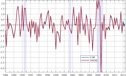
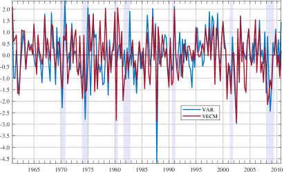
Appendix F Factor Augment VAR models

F1 On the relation between FAVAR and DFM

Consider the FAVAR model proposed by Bernanke et al. (2005):

$$\mathbf{w}_{t}=\bm{L}^{f}\mathbf{f}_{t}+\bm{L}^{z}\mathbf{z}_{t}+\mathbf{e}_{t},\qquad\bm{\Psi}(L)\begin{bmatrix}\mathbf{f}_{t}\\ \mathbf{z}_{t}\end{bmatrix}=\mathbf{v}_{t},$$ (F1)

where $\mathbf{z}_{t}$ is an $m$-dimensional vector of observable economic variables of interest, $\mathbf{f}_{t}$ is a $k$-dimensional vector of latent factors summarising additional information contained in the $N$-dimensional vector $\mathbf{w}_{t}$. In this setting $\mathbf{e}_{t}$ is the idiosyncratic component of $\mathbf{w}_{t}$ and $\mathbf{v}_{t}$ is a white noise process containing the structural shocks that we are interested in and it is of dimension $k+m\ll N$.

Following Stock and Watson (2016, Section 5.2), let

$$\mathbf{x}_{t}=\begin{bmatrix}\mathbf{w}_{t}\\ \mathbf{z}_{t}\end{bmatrix}\qquad\mathrm{and}\qquad\bar{\mathbf{F}}_{t}=\begin{bmatrix}\mathbf{f}_{t}\\ \mathbf{z}_{t}\end{bmatrix},$$

where ${\mathbf{x}}_{t}$ is the vector of all observed time series of dimension $n=N+m$ and $\bar{\mathbf{F}}_{t}$ is $(m+k)$-dimensional. Then, we can rewrite (F1) as:

$${\mathbf{x}}_{t}=\bar{\bm{\Lambda}}\bar{\mathbf{F}}_{t}+\bar{\bm{\xi}}_{t},\qquad\bm{\Psi}(L)\bar{\mathbf{F}}_{t}=\mathbf{v}_{t},$$ (F2)

where:

$$\bar{\bm{\Lambda}}=\begin{bmatrix}\bm{L}^{f}&\bm{L}^{z}\\ \mathbf{0}_{m\times r}&\mathbf{I}_{m}\end{bmatrix}\qquad\mathrm{and}\qquad\bar{\bm{\xi}}_{t}=\begin{bmatrix}\mathbf{e}_{t}\\ \mathbf{0}_{m\times 1}\end{bmatrix}.$$

On the other hand the DFM reads

$$\mathbf{x}_{t}=\bm{\Lambda}\mathbf{F}_{t}+\bm{\xi}_{t},\qquad\mathbf{A}(L)\mathbf{F}_{t}=\mathbf{K}\mathbf{u}_{t}.$$ (F3)

Therefore, the FAVAR (F2) is a restricted version of the DFM (F3), where the variables $\mathbf{z}_{t}$ have unit factor loadings and zero idiosyncratic component and the number of factors is $r=k+m$, which is equal to the number of common shocks, i.e. in (F3) we also impose $r=q$ and thus $\mathbf{K}=\mathbf{I}_{r}$. In other words in a FAVAR the variables of interest $\mathbf{z}_{t}$ are considered as “observable” factors. Although the FAVAR has been mainly studied in a stationary setting, the same reasoning applies if we have non-stationary data. Note that deterministic linear trends can also be included in the FAVAR as we discuss in the next section.

F2 FAVAR estimation

Let $y_{it}$ be the observed data, then in our framework the FAVAR is written as

$$y_{it} =a_{i}+b_{i}t+x_{it},$$

$$x_{it} =(\bm{l}_{i}^{f^{\prime}}\quad\bm{l}_{i}^{z^{\prime}})(\mathbf{f}_{t}^{\prime}\quad\mathbf{z}_{t}^{\prime})^{\prime}+\xi_{it},$$

$$\bm{\Psi}(L)(\mathbf{f}_{t}^{\prime}\quad\mathbf{z}_{t}^{\prime})^{\prime} =\mathbf{v}_{t},$$

where $\mathbf{z}_{t}$ are the “observed” common factors, and $\mathbf{f}_{t}$ are the “unobserved” common factors. The model is estimated as follows:

1. estimate the unobserved common factors $\widehat{\mathbf{f}}_{t}$ from $\mathbf{y}_{t}=(y_{1t}\cdots y_{nt})^{\prime}$ as explained in Section 3, thus de-trending series first (if needed);

2. estimate $\widehat{\bm{\Psi}}(L)$ by fitting either a VECM on $(\Delta\widehat{\mathbf{f}}_{t}^{\prime}\quad\Delta{\mathbf{z}}_{t}^{\prime})^{\prime}$ or an unrestricted VAR on $(\widehat{\mathbf{f}}_{t}^{\prime}\quad{\mathbf{z}}_{t}^{\prime})^{\prime}$ as explained in Section 3;

3. estimate $(\widehat{\bm{l}}_{i}^{f^{\prime}}\quad\widehat{\bm{l}}_{i}^{z^{\prime}})$ by regressing $\Delta y_{it}$ onto a constant and the vector $(\Delta\mathbf{f}_{t}^{\prime}\quad\Delta\widehat{\mathbf{z}}_{t}^{\prime})^{\prime}$;

4. estimate IRFs as $(\widehat{\bm{l}}_{i}^{f^{\prime}}\quad\widehat{\bm{l}}_{i}^{z^{\prime}})[\widehat{\bm{\Psi}}(L)]^{-1}$.

In contrast, in the approach by Forni et al. (2014) the factors are extracted directly from the observed data $y_{it}$, without controlling for the presence of possible deterministic linear trends. Therefore, the FAVAR is written as

$$y_{it}=(\bm{l}_{i}^{f^{\prime}}\quad\bm{l}_{i}^{z^{\prime}})(\mathbf{f}_{t}^{\prime}\quad\mathbf{z}_{t}^{\prime})^{\prime}+\xi_{it}.$$

The model is estimated as follows:

1. estimate the unobserved common factors from PC analysis of $\mathbf{y}_{t}=(y_{1t}\cdots y_{nt})^{\prime}$ as in Bai (2004);

2. estimate an unrestricted VAR on $(\widehat{\mathbf{f}}_{t}^{\prime}\quad{\mathbf{z}}_{t}^{\prime})^{\prime}$ as explained in Section 3 to get $\widehat{\bm{\Psi}}(L)$;

3. estimate $(\widehat{\bm{l}}_{i}^{f^{\prime}}\quad\widehat{\bm{l}}_{i}^{z^{\prime}})$ by regressing $\Delta y_{it}$ onto a constant and the vector $(\Delta\mathbf{f}_{t}^{\prime}\quad\Delta\widehat{\mathbf{z}}_{t}^{\prime})^{\prime}$;

4. estimate IRFs as $(\widehat{\bm{l}}_{i}^{f^{\prime}}\quad\widehat{\bm{l}}_{i}^{z^{\prime}})[\widehat{\bm{\Psi}}(L)]^{-1}$.

References

- Aastveit (2014) Aastveit, K. A. (2014). Oil price shocks in a data-rich environment. Energy Economics 45, 268–279.
- Ahn and Horenstein (2013) Ahn, S. C. and A. R. Horenstein (2013). Eigenvalue ratio test for the number of factors. Econometrica 81, 1203–1227.
- Alessi et al. (2010) Alessi, L., M. Barigozzi, and M. Capasso (2010). Improved penalization for determining the number of factors in approximate static factor models. Statistics and Probability Letters 80, 1806–1813.
- Alessi and Kerssenfischer (2019) Alessi, L. and M. Kerssenfischer (2019). The response of asset prices to monetary policy shocks: Stronger than thought. Journal of Applied Econometrics 34(5), 661–672.
- Altissimo et al. (2010) Altissimo, F., R. Cristadoro, M. Forni, M. Lippi, and G. Veronese (2010). New eurocoin: Tracking economic growth in real time. The Review of Economics and Statistics 92, 1024–1034.
- Amengual and Watson (2007) Amengual, D. and M. W. Watson (2007). Consistent estimation of the number of dynamic factors in a large and panel. Journal of Business and Economic Statistics 25, 91–96.
- An et al. (2014) An, L., X. Jin, and X. Ren (2014). Are the macroeconomic effects of oil price shock symmetric? A Factor-Augmented Vector Autoregressive approach. Energy Economics 45, 217–228.
- Anderson and Deistler (2008) Anderson, B. D. and M. Deistler (2008). Generalized linear dynamic factor models-A structure theory. In Proceedings of the 47th IEEE Conference on Decision and Control, pp. 1980–1985.
- Bai (2003) Bai, J. (2003). Inferential theory for factor models of large dimensions. Econometrica 71, 135–171.
- Bai (2004) Bai, J. (2004). Estimating cross-section common stochastic trends in nonstationary panel data. Journal of Econometrics 122, 137–183.
- Bai and Ng (2002) Bai, J. and S. Ng (2002). Determining the number of factors in approximate factor models. Econometrica 70, 191–221.
- Bai and Ng (2004) Bai, J. and S. Ng (2004). A PANIC attack on unit roots and cointegration. Econometrica 72, 1127–1177.
- Bai and Ng (2006) Bai, J. and S. Ng (2006). Confidence intervals for diffusion index forecasts and inference for factor augmented regressions. Econometrica 74, 1133–1150.
- Bai and Ng (2007) Bai, J. and S. Ng (2007). Determining the number of primitive shocks in factor models. Journal of Business and Economic Statistics 25, 52–60.
- Bai and Ng (2008) Bai, J. and S. Ng (2008). Forecasting economic time series using targeted predictors. Journal of Econometrics 146(2), 304–317.
- Bai and Wang (2015) Bai, J. and P. Wang (2015). Identification and bayesian estimation of dynamic factor models. Journal of Business & Economic Statistics 33, 221–240.
- Banerjee et al. (2017) Banerjee, A., M. Marcellino, and I. Masten (2017). Structural FECM: Cointegration in large-scale structural FAVAR models. Journal of Applied Econometrics 32, 1069–1086.
- Barigozzi et al. (2014) Barigozzi, M., A. M. Conti, and M. Luciani (2014). Do euro area countries respond asymmetrically to the common monetary policy? Oxford Bulletin of Economics and Statistics 76, 693–714.
- Barigozzi et al. (2020) Barigozzi, M., M. Lippi, and M. Luciani (2020). Cointegration and error correction mechanisms for singular stochastic vectors. Econometrics 8(1), 1–23.
- Barsky and Kilian (2002) Barsky, R. B. and L. Kilian (2002). Do we really know that oil caused the great stagflation? A monetary alternative. In NBER Macroeconomics Annual 2001, Volume 16. MIT Press.
- Barsky and Sims (2011) Barsky, R. B. and E. R. Sims (2011). News shocks and business cycles. Journal of Monetary Economics 58(3), 273–289.
- Baumeister and Hamilton (2019) Baumeister, C. and J. D. Hamilton (2019). Structural interpretation of vector autoregressions with incomplete identification: Revisiting the role of oil supply and demand shocks. American Economic Review 109, 1873–1910.
- Beaudry and Portier (2006) Beaudry, P. and F. Portier (2006). Stock prices, news, and economic fluctuations. American Economic Review 96(4), 1293–1307.
- Beaudry and Portier (2014) Beaudry, P. and F. Portier (2014). News-Driven Business Cycles: Insights and Challenges. Journal of Economic Literature 52(4), 993–1074.
- Bernanke et al. (2005) Bernanke, B. S., J. Boivin, and P. S. Eliasz (2005). Measuring the effects of monetary policy: A Factor-Augmented Vector Autoregressive (FAVAR) approach. The Quarterly Journal of Economics 120, 387–422.
- Blanchard and Gali (2009) Blanchard, O. J. and J. Gali (2009). The macroeconomic effects of oil price shocks: Why are the 2000s so different from the 1970s? In J. Gali and M. J. Gertler (Eds.), International Dimensions of Monetary Policy, pp. 373–421. National Bureau of Economic Research, Inc.
- Blanchard et al. (2013) Blanchard, O. J., J.-P. L’Huillier, and G. Lorenzoni (2013). News, Noise, and Fluctuations: An Empirical Exploration. American Economic Review 103(7), 3045–3070.
- Boivin and Ng (2006) Boivin, J. and S. Ng (2006). Are more data always better for factor analysis? Journal of Econometrics 127, 169–194.
- Caldara et al. (2019) Caldara, D., M. Cavallo, and M. Iacoviello (2019). Oil price elasticities and oil price fluctuations. Journal of Monetary Economics 103, 1–20.
- Conflitti and Luciani (2019) Conflitti, C. and M. Luciani (2019). Oil price pass-through into core inflation. The Energy Journal 40(6), 221–247.
- Cristadoro et al. (2005) Cristadoro, R., M. Forni, L. Reichlin, and G. Veronese (2005). A core inflation indicator for the euro area. Journal of Money Credit and Banking 37(3), 539–560.
- Dahlhaus (2017) Dahlhaus, T. (2017). Conventional monetary policy transmission during financial crises: an empirical analysis. Journal of Applied Econometrics 32, 401–421.
- Eickmeier (2009) Eickmeier, S. (2009). Comovements and heterogeneity in the euro area analyzed in a non-stationary dynamic factor model. Journal of Applied Econometrics 24, 933–959.
- Engle and Granger (1987) Engle, R. F. and C. W. J. Granger (1987). Cointegration and error correction: Representation, estimation, and testing. Econometrica 55, 251–76.
- Fan et al. (2013) Fan, J., Y. Liao, and M. Mincheva (2013). Large covariance estimation by thresholding principal orthogonal complements. Journal of the Royal Statistical Society: Series B (Statistical Methodology) 75, 603–680.
- Forni and Gambetti (2010) Forni, M. and L. Gambetti (2010). The dynamic effects of monetary policy: A structural factor model approach. Journal of Monetary Economics 57, 203–216.
- Forni et al. (2014) Forni, M., L. Gambetti, and L. Sala (2014). No news in business cycles. Economic Journal 124, 1168–1191.
- Forni et al. (2009) Forni, M., D. Giannone, M. Lippi, and L. Reichlin (2009). Opening the black box: Structural factor models versus structural VARs. Econometric Theory 25, 1319–1347.
- Forni et al. (2018) Forni, M., A. Giovannelli, M. Lippi, and S. Soccorsi (2018). Dynamic factor model with infinite–dimensional factor space: Forecasting. Journal of Applied Econometrics 33(5), 625–642.
- Forni et al. (2000) Forni, M., M. Hallin, M. Lippi, and L. Reichlin (2000). The Generalized Dynamic Factor Model: Identification and estimation. The Review of Economics and Statistics 82, 540–554.
- Forni et al. (2005) Forni, M., M. Hallin, M. Lippi, and L. Reichlin (2005). The Generalized Dynamic Factor Model: One sided estimation and forecasting. Journal of the American Statistical Association 100, 830–840.
- Forni et al. (2017) Forni, M., M. Hallin, M. Lippi, and P. Zaffaroni (2017). Dynamic factor models with infinite dimensional factor space: Asymptotic analysis. Journal of Econometrics 199, 74–92.
- Forni and Lippi (2001) Forni, M. and M. Lippi (2001). The Generalized Dynamic Factor Model: Representation theory. Econometric Theory 17, 1113–1141.
- Gegenbach et al. (2015) Gegenbach, C., J.-P. Urbain, and J. Westerlund (2015). Error correction testing in panels with common stochastic trends. Journal of Applied Econometrics 31, 982–1004.
- Giannone et al. (2005) Giannone, D., L. Reichlin, and L. Sala (2005). Monetary policy in real time. In M. Gertler and K. Rogoff (Eds.), NBER Macroeconomics Annual 2004. MIT Press.
- Giannone et al. (2008) Giannone, D., L. Reichlin, and D. Small (2008). Nowcasting: The real-time informational content of macroeconomic data. Journal of Monetary Economics 55, 665–676.
- Gonzalo (1994) Gonzalo, J. (1994). Five alternative methods of estimating long-run equilibrium relationships. Journal of Econometrics 60, 203–233.
- Hallin and Liška (2007) Hallin, M. and R. Liška (2007). Determining the number of factors in the general dynamic factor model. Journal of the American Statistical Association 102, 603–617.
- Hamilton (1983) Hamilton, J. D. (1983). Oil and the macroeconomy since World War II. Journal of Political Economy 91, 228–248.
- Hamilton (1994) Hamilton, J. D. (1994). Time Series Analysis. Princeton, New Jersey: Princeton University Press.
- Han (2018) Han, X. (2018). Estimation and inference of dynamic structural factor models with over-identifying restrictions. Journal of Econometrics 202, 125–147.
- Johansen (1995) Johansen, S. (1995). Likelihood-based inference in cointegrated vector autoregressive models (First ed.). Oxford: Oxford University Press.
- Juvenal and Petrella (2015) Juvenal, L. and I. Petrella (2015). Speculation in the oil market. Journal of Applied Econometrics 30, 621–649.
- Kilian (2008) Kilian, L. (2008). Exogenous oil supply shocks: how big are they and how much do they matter for the U.S. economy? Review of Economics and Statistics 90, 216–240.
- Kilian (2009) Kilian, L. (2009). Not all oil price shocks are alike: Disentangling demand and supply shocks in the crude oil market. American Economic Review 99, 1053–1069.
- Kilian and Lütkepohl (2017) Kilian, L. and H. Lütkepohl (2017). Structural Vector Autoregressive Analysis. Cambridge University Press.
- Kilian and Vega (2011) Kilian, L. and C. Vega (2011). Do energy prices respond to U.S. macroeconomic news? A test of the hypothesis of predetermined energy prices. Review of Economics and Statistics 93, 660–671.
- Kurmann and Otrok (2013) Kurmann, A. and C. Otrok (2013). News Shocks and the Slope of the Term Structure of Interest Rates. American Economic Review 103(6), 2612–2632.
- Luciani (2014) Luciani, M. (2014). Forecasting with approximate dynamic factor models: The role of non-pervasive shocks. International Journal of Forecasting 30, 20–29.
- Luciani (2015) Luciani, M. (2015). Monetary policy and the housing market: A structural factor analysis. Journal of Applied Econometrics 30, 199–218.
- McCracken and Ng (2020) McCracken, M. and S. Ng (2020). FRED-QD: A quarterly database for macroeconomic research. Working Paper 26872, NBER.
- Onatski (2009) Onatski, A. (2009). Testing hypotheses about the number of factors in large factor models. Econometrica 77, 1447–1479.
- Onatski (2010) Onatski, A. (2010). Determining the number of factors from empirical distribution of eigenvalues. The Review of Economics and Statistics 92, 1004–1016.
- Onatski and Wang (2020) Onatski, A. and C. Wang (2020). Spurious factor analysis. Cambridge-INET Working Paper Series 2020/01, Cambridge University.
- Paruolo (1997) Paruolo, P. (1997). Asymptotic inference on the moving average impact matrix in cointegrated VAR systems. Econometric Theory 13, 79–118.
- Phillips (1991) Phillips, P. C. (1991). Optimal inference in cointegrated systems. Econometrica 59, 238–306.
- Phillips (1998) Phillips, P. C. (1998). Impulse response and forecast error variance asymptotics in nonstationary VARs. Journal of Econometrics 83, 21–56.
- Phillips and Durlauf (1986) Phillips, P. C. and S. N. Durlauf (1986). Multiple time series regression with integrated processes. The Review of Economic Studies 53, 473–495.
- Phillips and Ouliaris (1988) Phillips, P. C. and S. Ouliaris (1988). Testing for cointegration using principal components methods. Journal of Economic Dynamics and Control 12, 205–230.
- Phillips and Solo (1992) Phillips, P. C. and V. Solo (1992). Asymptotics for linear processes. The Annals of Statistics 20, 971–1001.
- Schmitt-Grohé and Uribe (2012) Schmitt-Grohé, S. and M. Uribe (2012, November). What’s News in Business Cycles. Econometrica 80(6), 2733–2764.
- Sims et al. (1990) Sims, C., J. H. Stock, and M. W. Watson (1990). Inference in linear time series models with some unit roots. Econometrica 58, 113–144.
- Stock and Watson (2002) Stock, J. H. and M. W. Watson (2002). Forecasting using principal components from a large number of predictors. Journal of the American Statistical Association 97, 1167–1179.
- Stock and Watson (2016) Stock, J. H. and M. W. Watson (2016). Dynamic factor models, factor-augmented vector autoregressions, and structural vector autoregressions in macroeconomics. In J. B. Taylor and H. Uhlig (Eds.), Handbook of Macroeconomics, Volume 2, pp. 415–525. Elsevier.
- Velu et al. (1986) Velu, R. P., G. C. Reinsel, and D. W. Wichern (1986). Reduced rank models for multiple time series. Biometrika 73, 105–118.
- Watson (1994) Watson, M. W. (1994). Vector autoregressions and cointegration. In R. Engle and D. McFadden (Eds.), Handbook of Econometrics, Volume IV. Elsevier Science.
- Yu et al. (2015) Yu, Y., T. Wang, and R. J. Samworth (2015). A useful variant of the Davis–Kahan theorem for statisticians. Biometrika 102, 315–323.