Rarefaction Waves of the Korteweg–de Vries Equation via Nonlinear Steepest Descent

Abstract.

We apply the method of nonlinear steepest descent to compute the long-time asymptotics of the Korteweg–de Vries equation with steplike initial data leading to a rarefaction wave. In addition to the leading asymptotic we also compute the next term in the asymptotic expansion of the rarefaction wave, which was not known before.

1. Introduction

In this paper we investigate the Cauchy problem for the Korteweg–de Vries (KdV) equation

(1.1) $$q_{t}(x,t)=6q(x,t)q_{x}(x,t)-q_{xxx}(x,t),\quad(x,t)\in\mathbb{R}\times\mathbb{R}_{+},$$

with steplike initial data $q(x,0)=q_{0}(x)$ satisfying

(1.2) $$\left\{\begin{array}[]{ll}q_{0}(x)\to 0,&\ \ \mbox{as}\ \ x\to+\infty,\\ q_{0}(x)\to c^{2},&\ \ \mbox{as}\ \ x\to-\infty.\end{array}\right.$$

This case is known as rarefaction problem. The corresponding long-time asymptotics of $q(x,t)$ as $t\to\infty$ are well understood on a physical level of rigor ([28, 20, 24]) and can be split into three main regions:

• In the region $x<-6c^{2}t$ the solution is asymptotically close to the background $c^{2}$.

• In the region $-6c^{2}t<x<0$ the solution can asymptotically be described by $-\frac{x}{6t}$.

• In the region $0<x$ the solution is asymptotically given by a sum of solitons.

This is illustrated in Figure 1. For the corresponding shock problem we refer to [2, 8, 13, 14, 18, 21, 27].

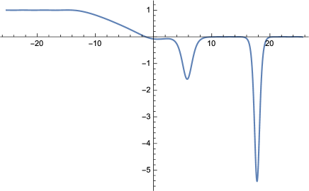
Figure 1. Numerically computed solution $q(x,t)$ of the KdV equation at time $t=1.5$, with initial condition $q_{0}(x)=\frac{1}{2}(1-\mathrm{erf}(x))-4\mathop{\mathrm{sech}}(x-1)$.

The aim of the present paper is to rigorously justify these results. Furthermore, we will also compute the second terms in the asymptotic expansion, which were, to the best of our knowledge, not obtained before. Our approach is based on the nonlinear steepest descent method for oscillatory Riemann–Hilbert (RH) problems. In turn, this approach rests on the inverse scattering transform for steplike initial data originally developed by Buslaev and Fomin [3] with later contributions by Cohen and Kappeler [4]. For recent developments and further information we refer to [9]. The application of the inverse scattering transform to the problem (1.1)–(1.2) (see [10], [11]) implies that the solution $q(x,t)$ of the Cauchy problem exists in the classical sense and is unique in the class

(1.3) $$\int_{0}^{\infty}|x|(|q(x,t)|+|q(-x,t)-c^{2}|)dx<\infty,\qquad\forall t\in\mathbb{R},$$

provided the initial data satisfy the following conditions: $q_{0}\in\mathcal{C}^{8}(\mathbb{R})$ and

(1.4) $$\int_{0}^{\infty}x^{4}\left(|q_{0}(x)|+|q_{0}(-x)-c^{2}|+|q^{(j)}(x)|\right)dx<\infty,\quad j=1,\dots,8.$$

To simplify considerations we will additionally suppose that the initial condition decays exponentially fast to the asymptotics:

(1.5) $$\int_{0}^{+\infty}\mathrm{e}^{\kappa x}(|q_{0}(x)|+|q_{0}(-x)-c^{2}|)dx<\infty,$$

for some small $\kappa>0$. We remark that by [26] the solution will be even real analytic under this assumption, but we will not need this fact.

This last assumption can be removed using analytic approximation of the reflection coefficient as demonstrated by Deift and Zhou [7] (see also [12, 22]), but we will not address this in the present paper. However, we emphasize that all known results concerning the asymptotic behavior of steplike solutions were obtained for the case of pure step initial data ($q_{0}(x)=0$ for $x>0$ and $q_{0}(x)=\pm c^{2}$ for $x\leq 0$) only. Moreover, those using the Riemann-Hilbert approach did not address the parametrix problem, which is one of the main contributions of the present paper.

As is known, the solution of the initial value problem (1.1), (1.4) can be computed by the inverse scattering transform from the right scattering data of the initial profile. Here the right scattering data are given by the reflection coefficient $R(k)$, $k\in\mathbb{R}$, a finite number of eigenvalues $-\kappa_{1}^{2}$, …, $-\kappa_{N}^{2}$, and positive norming constants $\gamma_{1},\dots,\gamma_{N}$. The difference with the decaying case $c=0$ consists of the fact, that the modulus of the reflection coefficient is equal to 1 on the interval $[-c,c]$. At the point $k=0$ the reflection coefficient takes the values $\pm 1$ (cf. [4]). The case $R(0)=-1$ known as the nonresonant case (which is generic), whereas the case $R(0)=1$ is called the resonant case. Note, that the right transmission coefficient $T(k)$ can be reconstructed uniquely from these data (cf. [3]).

Our main results is the following

Theorem 1.1.

Let the initial data $q_{0}(x)\in\mathcal{C}^{8}(\mathbb{R})$ of the Cauchy problem (1.1)–(1.2) satisfy (1.5). Let $q(x,t)$ be the solution of this problem. Then for arbitrary small $\epsilon_{j}>0$, $j=1,2,3$, and for $\xi=\frac{x}{12t}$, the following asymptotics are valid as $t\to\infty$ uniformly with respect to $\xi$:

A. In the domain $(-6c^{2}+\epsilon_{1})t<x<-\epsilon_{1}t$:

(1.6) $$q(x,t)=-\frac{x+Q(\xi)}{6t}(1+O(t^{-1/3})),\quad\mbox{as}\ t\to+\infty,$$

where

(1.7) $$Q(\xi)=\frac{2}{\pi}\int_{-\sqrt{-2\xi}}^{\sqrt{-2\xi}}\left(\frac{d}{ds}\log R(s)-4\mathrm{i}\sum_{j=1}^{N}\frac{\kappa_{j}}{s^{2}+\kappa_{j}^{2}}\right)\frac{ds}{\sqrt{s^{2}+2\xi}}\mp\frac{1}{2\sqrt{-2\xi}},$$

with $\pm$ corresponding to the resonant/nonresonant case, respectively.

B. In the domain $x<(-6c^{2}-\epsilon_{2})t$ in the nonresonant case:

(1.8) $$q(x,t)=c^{2}+\sqrt{\frac{4\nu\tau}{3t}}\sin(16t\tau^{3}-\nu\log(192t\tau^{3})+\delta)(1+o(1)),$$

where $\tau=\tau(\xi)=\sqrt{\frac{c^{2}}{2}-\xi}$, $\nu=\nu(\xi)=-\frac{1}{2\pi}\log\left(1-|R(\tau)|^{2}\right)$ and

$$\delta(\xi)= -\frac{3\pi}{4}+\arg(R(\tau)-2T(\tau)+\Gamma(\mathrm{i}\nu))$$

$$-\frac{1}{\pi}\int_{\mathbb{R}\setminus[-\tau,\tau]}\log\frac{1-|R(s)|^{2}}{1-|R(\tau)|^{2}}\,\frac{s\,ds}{s^{2}-c^{2}-(\frac{c^{2}}{2}+\xi)^{1/2}(c^{2}-s^{2})^{1/2}}.$$

Here $\Gamma$ is the Gamma function.

C. In the domain $x>\epsilon_{3}t$:

$$q(x,t)=-\sum_{j=1}^{N}\frac{2\kappa_{j}^{2}}{\cosh^{2}\left(\kappa_{j}x-4\kappa_{j}^{3}t-\frac{1}{2}\log\frac{\gamma_{j}}{2\kappa_{j}}-\sum_{i=j+1}^{N}\log\frac{\kappa_{i}-\kappa_{j}}{\kappa_{i}+\kappa_{j}}\right)}+O(\mathrm{e}^{-\epsilon_{3}t/2}).$$

We should remark that our results do not cover the two transitional regions: $0\approx x$ near the leading wave front, and $x\approx-6c^{2}t$ near the back wave front. Since the error bounds obtained from the RH method break down near these edges, a rigorous justification is beyond the scope of the present paper.

Our paper is organized as follows: Section 2 provides some necessary information about the inverse scattering transform with steplike backgrounds and formulates the initial vector RH problems. In Section 3 we study the soliton region. In Section 4 the initial RH problem is reduced to a ”model” problem in the domain $-6c^{2}t<x<0$. It is solved in Section 5, and the question of a suitable parametrix is discussed in Section 6. Justification of the asymptotical formula (1.6)–(1.7) is given in Section 7. In Section 8 we establish the asymptotics in the dispersive region $x<-6c^{2}t$.

2. Statement of the RH problem and the first conjugation step

Let $q(x,t)$ be the solution of the Cauchy problem (1.1), (1.4) and consider the underlying spectral problem

(2.1) $$(H(t)f)(x):=-\frac{d^{2}}{dx^{2}}f(x)+q(x,t)f(x)=\lambda f(x),\qquad x\in\mathbb{R}.$$

In order to set up the respective Riemann–Hilbert (RH) problems we recall some facts from scattering theory with steplike backgrounds. We refer to [9] for proofs and further details.

Throughout this paper we will use the following notations: Set $\mathcal{D}:=\mathbb{C}\setminus\Sigma$, where

$$\Sigma=\Sigma_{U}\cup\Sigma_{L},\quad\Sigma_{U}=\{\lambda^{U}=\lambda+\mathrm{i}0,\lambda\in[0,\infty)\},\quad\Sigma_{L}=\{\lambda^{L}=\lambda-\mathrm{i}0,\lambda\in[0,\infty)\}$$

(throughout this paper the indices $U$ and $L$ will stand for ”upper” and ”lower”). That is, we treat the boundary of the domain $\mathcal{D}$ as consisting of the two sides of the cut along the interval $[0,\infty)$, with different points $\lambda^{U}$ and $\lambda^{L}$ on different sides. In equation (2.1) the spectral parameter $\lambda$ belongs to the set $\mathop{\mathrm{clos}}(\mathcal{D})$, where $\mathop{\mathrm{clos}}(\mathcal{D})=\mathcal{D}\cup\Sigma_{U}\cup\Sigma_{L}$. Along with $\lambda$ we will use two more spectral parameters

$$k=\sqrt{\lambda},\quad k_{1}=\sqrt{\lambda-c^{2}},\quad\mbox{where}\ \ k>0\ \ \mbox{and}\ \ k_{1}>0,\ \ \mbox{ for }\ \lambda^{U}>c^{2}.$$

The functions $k_{1}(\lambda)$ and $k(\lambda)$ conformally map the domain $\mathcal{D}$ onto $\mathfrak{D}_{1}:=\mathbb{C}^{+}\setminus(0,\mathrm{i}c]$ and $\mathfrak{D}:=\mathbb{C}^{+}$, respectively. Since there is a bijection between the closed domains $\mathop{\mathrm{clos}}\mathcal{D}$, $\mathop{\mathrm{clos}}\mathfrak{D}=\mathbb{C}^{+}\cup\mathbb{R}$ and $\mathop{\mathrm{clos}}\mathfrak{D}_{1}=\mathfrak{D}_{1}\cup\mathbb{R}\cup[0,\mathrm{i}c]_{r}\cup[0,\mathrm{i}c]_{l}$, we will use the ambiguous notation $f(k)$ or $f(k_{1})$ or $f(\lambda)$ for the same value of an arbitrary function $f(\lambda)$ in these respective coordinates. Here the indices $l$ and $r$ are associated with the right and the left sides of the cut. In particular, if $k>0$ corresponds to $\lambda^{U}$ then $-k$ corresponds to $\lambda^{L}$, and for functions defined on the set $\Sigma$ we will sometimes use the notation $f(k)$ and $f(-k)$ to indicate the values at symmetric points $\lambda^{U}$ and $\lambda^{L}$.

Since the potential $q(x,t)$ satisfies (1.3), the following facts are valid for the operator $H(t)$ ([9]):

Theorem 2.1.

• The spectrum of $H(t)$ consists of an absolutely continuous part $\mathbb{R}_{+}$ plus a finite number of negative eigenvalues $\lambda_{1}<\cdots<\lambda_{N}<0$. The (absolutely) continuous spectrum consists of a part $[0,c^{2}]$ of multiplicity one and a part $[c^{2},\infty)$ of multiplicity two. In terms of the variables $k$ and $k_{1}$, the continuous spectrum corresponds to $k\in\mathbb{R}$, and the spectrum of multiplicity two to $k_{1}\in\mathbb{R}$.

• Equation (2.1) has two Jost solutions $\phi(\lambda,x,t)$ and $\phi_{1}(\lambda,x,t)$, satisfying the conditions

  $$\lim_{x\to+\infty}\mathrm{e}^{-\mathrm{i}kx}\phi(\lambda,x,t)=\lim_{x\to-\infty}\mathrm{e}^{\mathrm{i}k_{1}x}\phi_{1}(\lambda,x,t)=1,\quad\mbox{for}\ \ \lambda\in\mathop{\mathrm{clos}}\mathcal{D}.$$

  The Jost solutions fulfill the scattering relations

  (2.2) $$T(\lambda,t)\phi_{1}(\lambda,x,t) =\overline{\phi(\lambda,x,t)}+R(\lambda,t)\phi(\lambda,x,t),\qquad k\in\mathbb{R},$$

  (2.3) $$T_{1}(\lambda,t)\phi(\lambda,x,t) =\overline{\phi_{1}(\lambda,x,t)}+R_{1}(\lambda,t)\phi_{1}(\lambda,x,t),\quad k_{1}\in\mathbb{R},$$

  where $T(\lambda,t)$, $R(\lambda,t)$ (resp., $T_{1}(\lambda,t)$, $R_{1}(\lambda,t)$) are the right (resp., the left) transmission and reflection coefficients.

• The Wronskian

  (2.4) $$W(\lambda,t)=\phi_{1}(\lambda,x,t)\phi^{\prime}(\lambda,x,t)-\phi_{1}^{\prime}(\lambda,x,t)\phi(\lambda,x,t)$$

  of the Jost solutions has simple zeros at the points $\lambda_{j}$. The only other possible zero is $\lambda=0$. The case $W(0,t)=0$ is known as the resonant case. In this case $R(0,t)=1$. In the nonresonant case, which is generic, $R(0,t)=-1$.

• The solutions $\phi(\lambda_{j},x,t)$ and $\phi_{1}(\lambda_{j},x,t)$ are the corresponding (linearly dependent) eigenfunctions of $H(t)$. The associated norming constants are

  (2.5) $$\gamma_{j}(t)=\left(\int_{\mathbb{R}}\phi^{2}(\lambda_{j},x,t)dx\right)^{-1},\quad\gamma_{j,1}(t)=\left(\int_{\mathbb{R}}\phi^{2}_{1}(\lambda_{j},x,t)dx\right)^{-1}.$$

• The function $T(\lambda,t)$ has a meromorphic extensions to the domain $\lambda\in\mathbb{C}\setminus[0,\infty)$ with simple poles at the points $\lambda_{1}$,…, $\lambda_{N}$. The only possible zero is at $\lambda=0$ in the nonresonant case. In the resonant case $T(\lambda,t)\neq 0$ for all $\lambda\in\mathop{\mathrm{clos}}(\mathcal{D})$.

• There is a symmetry $T(\lambda^{U},t)=\overline{T(\lambda^{L},t)}$, $T_{1}(\lambda^{U},t)=\overline{T_{1}(\lambda^{L},t)}$, $R(\lambda^{U},t)=\overline{R(\lambda^{L},t)}$ for $k\in\mathbb{R}$, i.e. for $\lambda\in\Sigma$. The same is valid for $\phi(\lambda,x,t)$ and $\phi_{1}(\lambda,x,t)$. Moreover, $\phi_{1}(\lambda,x,t)\in\mathbb{R}$ for $k\in[-c,c]$ and $R_{1}(\lambda^{U},t)=\overline{R_{1}(\lambda^{L},t)}$ for $k_{1}\in\mathbb{R}$.

• The following identities are valid on the continuous spectrum:

  (2.6) $$-\frac{T_{1}(\lambda,t)}{\overline{T_{1}(\lambda,t)}}=\frac{T(\lambda,t)}{\overline{T(\lambda,t)}}=R(\lambda,t)\mathrm{e}^{2\mathrm{i}\arg k},\ \mbox{for}\ \ k\in[-c,c],$$

  and for $k_{1}\in\mathbb{R}$:

  (2.7) $$1-|R(\lambda,t)|^{2}=1-|R_{1}(\lambda,t)|^{2}=T_{1}(\lambda,t)\overline{T(\lambda,t)},$$

  $$R_{1}(\lambda,t)\overline{T(\lambda,t)}+\overline{R(\lambda,t)}T(\lambda,t)=0.$$

  Here $\arg k=\pi$ as $k<0$.

• The spectrum is time independent and the time evolution of the scattering data is given by ([11, 16, 17])

  $$R(\lambda,t) =R(k)\mathrm{e}^{8\mathrm{i}k^{3}t},\quad\quad\qquad k\in\mathbb{R},$$

  (2.8) $$\chi(\lambda,t) =\chi(k)\mathrm{e}^{-8\mathrm{i}tk_{1}^{3}-12\mathrm{i}tk_{1}c^{2}},\qquad k\in[-c,c],$$

  $$R_{1}(\lambda,t) =R_{1}(k_{1})\mathrm{e}^{-8\mathrm{i}tk_{1}^{2}-12\mathrm{i}tk_{1}c^{2}},\qquad k_{1}\in\mathbb{R},$$

  $$\gamma_{1,j}(t) =\gamma_{1,j}\mathrm{e}^{-8\kappa_{1,j}^{3}t+12c^{2}\kappa_{1,j}t},\qquad\gamma_{j}(t)=\gamma_{j}\mathrm{e}^{8\kappa_{j}^{3}t},$$

  where

  (2.9) $$\chi(\lambda,t):=-\overline{T_{1}(\lambda,t)}T(\lambda,t);\ \ \chi(k)=\chi(\lambda(k),0);\ R(k)=R(\lambda(k),0);$$

  (2.10) $$\gamma_{1,j}=\gamma_{1,j}(0);\ \gamma_{j}=\gamma_{j}(0);\ 0<\kappa_{j}=\sqrt{-\lambda_{j}};\ \kappa_{1,j}=\sqrt{\kappa_{j}^{2}+c^{2}}.$$

• Under the assumption (1.5) with $0<\kappa<\kappa_{N}$ the solution $\overline{\phi(\lambda,x,0)}$ has an analytical continuation to a subdomain $\mathcal{D}_{\kappa}\subset\mathcal{D}$, where $\mathcal{D}_{\kappa}=\{\lambda(k):\,0<\mathop{\mathrm{Im}}k<\kappa\}$. Accordingly, the function $R(k)$ has a holomorphic continuation to the strip $0<\mathop{\mathrm{Im}}k<\kappa$, continuous up to the boundary $\mathop{\mathrm{Im}}k=0$. The transmission coefficient as a function of $k$ always has an analytical continuation in $\mathbb{C}^{+}$, and is holomorphic in the strip and continuous up to the boundary $\mathbb{R}$. Identity (2.2) remains valid in the strip.

• The solution $q(x,t)$ of the initial value problem (1.1)–(1.4) can be uniquely recovered from either the right initial scattering data

  $$\{R(k),\ \ k\in\mathbb{R};\ \ \lambda_{j}=-\kappa_{j}^{2},\ \gamma_{j}>0,\ j=1,\dots,N\},$$

  or from the left initial scattering data

  $$\{R_{1}(k_{1}),\ \ k_{1}\in\mathbb{R};\ \ \chi(k),\ k\in[-c,c];\ \ \lambda_{j},\ \gamma_{1,j}>0,\ \ j=1,\dots,N\}.$$

These properties allow us to formulate two vector RH problems. One of them is connected with the right scattering data, another one with the left one. To this end we introduce a vector function

(2.11) $$m(\lambda,x,t)=\begin{pmatrix}T(\lambda,t)\phi_{1}(\lambda,x,t)\mathrm{e}^{\mathrm{i}kx},&\phi(\lambda,x,t)\mathrm{e}^{-\mathrm{i}kx}\end{pmatrix}$$

on $\mathop{\mathrm{clos}}\mathcal{D}$. By Theorem 2.1 this function is meromorphic in $\mathcal{D}$ with simple poles at the points $\lambda_{j}$, and continuous up to the boundary $\Sigma$. We regard it as a function of $k\in\overline{\mathbb{C}_{+}}$ (with $\overline{\mathbb{C}_{+}}$ the closed upper half-plane), keeping $x$ and $t$ as parameters. Accordingly we will write $m(k):=m(\lambda(k),x,t)$. This vector function has the following asymptotical behavior (cf. [8] and [9], Lemma 4.3) as $k\to\infty$ in any direction of $\overline{\mathbb{C}_{+}}$:

(2.12) $$m(k)=\begin{pmatrix}m_{1}(k)&m_{2}(k)\end{pmatrix}=\begin{pmatrix}1&1\end{pmatrix}-\frac{1}{2\mathrm{i}k}\int_{x}^{+\infty}q(y,t)dy\begin{pmatrix}-1&1\end{pmatrix}+O\left(\frac{1}{k^{2}}\right),$$

and

(2.13) $$m_{1}(k)m_{2}(k)=T(k)\phi(k,x,t)\phi_{1}(k,x,t)=1+\frac{q(x,t)}{2k^{2}}+O(\frac{1}{k^{4}}).$$

Extend the definition of $m(k)$ to $\mathbb{C}^{-}$ using the symmetry condition

(2.14) $$m(k)=m(-k)\sigma_{1},$$

where

$$\sigma_{1}=\begin{pmatrix}0&1\\ 1&0\end{pmatrix},\quad\sigma_{2}=\begin{pmatrix}0&-\mathrm{i}\\ \mathrm{i}&0\end{pmatrix},\quad\sigma_{3}=\begin{pmatrix}1&0\\ 0&-1\end{pmatrix}$$

are the Pauli matrices. After this extension the function $m$ has a jump along the real axis. We consider the real axis as a contour with the natural orientation from minus to plus infinity, and denote by $m_{+}(k)$ (resp. $m_{-}(k)$) the limiting values of $m(k)$ from the upper (resp. lower) half-plane.

Theorem 2.2.

Let $\{R(k),\,k\in\mathbb{R};\ \lambda_{j}=-\kappa_{j}^{2},\ \gamma_{j}>0,\ j=1,\dots,N\}$ be the right scattering data for the initial datum $q_{0}(x)$, satisfying condition (1.4), and let $q(x,t)$ be the unique solution of the Cauchy problem (1.1), (1.4). Then the vector-valued function $m(k)$ defined by (2.11) and (2.14) is the unique solution of the following vector Riemann–Hilbert problem:

Find a vector-valued function $m(k)$, which is meromorphic away from the contour $\mathbb{R}$ with continuous limits from both sides of the contour and satisfies:

1. The jump condition $m_{+}(k)=m_{-}(k)v(k)$, where

   (2.15) $$v(k):=v(\lambda(k),x,t)=\begin{pmatrix}1-\lvert R(k)\rvert^{2}&-\overline{R(k)}\mathrm{e}^{-2t\Phi(k)}\\[2.84526pt] R(k)\mathrm{e}^{2t\Phi(k)}&1\end{pmatrix},\quad k\in\mathbb{R};$$

2. the pole conditions

   (2.16) $$\operatorname{Res}_{\mathrm{i}\kappa_{j}}m(k) =\lim_{k\to\mathrm{i}\kappa_{j}}m(k)\begin{pmatrix}0&0\\ \mathrm{i}\gamma_{j}\mathrm{e}^{2t\Phi(\mathrm{i}\kappa_{j})}&0\end{pmatrix},$$

   $$\operatorname{Res}_{-\mathrm{i}\kappa_{j}}m(k) =\lim_{k\to-\mathrm{i}\kappa_{j}}m(k)\begin{pmatrix}0&-\mathrm{i}\gamma_{j}\mathrm{e}^{-2t\Phi(\mathrm{i}\kappa_{j})}\\ 0&0\end{pmatrix};$$

3. the symmetry condition (2.14);

4. the normalization condition

   (2.17) $$m(k)=\begin{pmatrix}1&1\end{pmatrix}+O(k^{-1}),\quad k\to\infty.$$

Here the phase $\Phi(k)=\Phi(k,x,t)$ in (2.15) is given by

$$\Phi(k)=4\mathrm{i}k^{3}+\mathrm{i}k\frac{x}{t}.$$

Remark 2.3.

Note that by property (2.6) we have $|R(k)|=1$ for $k\in[-c,c]$ implying

$$v(k)=\begin{pmatrix}0&-\overline{R(k)}\mathrm{e}^{-2t\Phi(k)}\\[2.84526pt] R(k)\mathrm{e}^{2t\Phi(k)}&1\end{pmatrix},\quad k\in[-c,c].$$

Proof of Theorem 2.2..

Since our further considerations mainly affect $k$, we drop $x$ and $t$ from our notation whenever possible. Let $m(k)$ be defined by (2.11). In the upper half-plane it is a meromorphic function, its first component $m_{1}(k)$ has simple poles at points $\mathrm{i}\kappa_{j}$, and the second component $m_{2}(k)$ is holomorphic one. Both components have continuous limits up to the boundary $\mathbb{R}$, moreover, for $k\in\mathbb{R}$ we have $m_{+}(-k)=\overline{m_{+}(k)}$. To compute the jump condition we observe that if $m_{+}=\big{(}T\phi_{1}z,\>\>\phi z^{-1}\big{)}$, where $z=\mathrm{e}^{\mathrm{i}kx}$, $k\in\mathbb{R}$, then by the symmetry condition $m_{-}=\big{(}\overline{\phi}z,\>\>\overline{T\phi_{1}}z^{-1}\big{)}$ at the same point $k\in\mathbb{R}$. Write $\big{(}\begin{smallmatrix}\alpha(k)&\beta(k)\\ \gamma(k)&\delta(k)\end{smallmatrix}\big{)}$ for the unknown jump matrix. Then

$$T\phi_{1}z=\overline{\phi}\,z\alpha+\overline{T\phi_{1}}z^{-1}\gamma,\qquad\phi\,z^{-1}=\overline{\phi}\,z\beta+\overline{T\phi_{1}}z^{-1}\delta.$$

Multiply the first equality by $z^{-1}$, the second one by $z$, and then conjugate both of them. We finally get

(2.18) $$\overline{\alpha}\phi=\overline{T\phi_{1}}-T\overline{\gamma}\phi_{1}z^{2},\qquad T\overline{\delta}\phi_{1}=\overline{\phi}-\overline{\beta}\phi z^{-2}.$$

Now divide the first of these equalities by $\overline{T}$ and compare it with (2.3) as $k_{1}\in\mathbb{R}$. From (2.7) it follows that $\alpha=T_{1}\overline{T}=1-|R|^{2}$, $\gamma z^{-2}=R$ if $k_{1}\in\mathbb{R}$. For $k\in[-c,c]$ we use the first equality of (2.18) taking into account that $\overline{\phi}_{1}=\phi_{1}$. Then by (2.6) $\overline{\alpha}\phi=\phi_{1}\overline{T}(1-\overline{\gamma}z^{2}R)$ and therefore $\alpha=0$, $\gamma z^{-2}=R$ if $k\in[-c,c]$. Taking into account (2.8) and $z=\mathrm{e}^{\mathrm{i}kx}$ we finally justify the $11$ and $21$ entries of the jump matrix (2.15). Comparing the second equality of (2.18) with (2.2) gives $\delta=1$ and $-\overline{\beta}z^{-2}=R$. This justifies the $12$ and $22$ entries.

The pole condition (2.16) is proved in [12] or in Appendix A of [8]. The symmetry condition holds by definition, and the normalization condition follows from (2.12).

It remains to prove that the solution of this RH problem is unique. Let $m(k)$ and $\tilde{m}(k)$ be two solutions. Then $\hat{m}(k)=m(k)-\tilde{m}(k)$ satisfies I–III (note, that condition II does not guarantee that $\hat{m}$ is a holomorphic solution!) and condition IV is replaced by $\hat{m}(k)=O(k^{-1})$. Therefore the function

$$F(k):=\hat{m}_{1}(k)\overline{\hat{m}_{1}(\overline{k})}+\hat{m}_{2}(k)\overline{\hat{m}_{2}(\overline{k})}$$

is a meromorphic in $\mathbb{C}^{+}$ with simple poles at the points $\mathrm{i}\kappa_{j}$ and with the asymptotical behavior $F(k)=O(k^{-2})$ as $k\to\infty$. Since $-\overline{k}=k$ for $k\in\mathrm{i}\mathbb{R}$ condition II implies

(2.19) $$\operatorname{Res}_{\mathrm{i}\kappa_{j}}F(k)=2\mathrm{i}\gamma_{j}|\hat{m}_{2}(\mathrm{i}\kappa_{j})|^{2}\mathrm{e}^{2t\Phi(\mathrm{i}\kappa_{j})}\in\mathrm{i}\mathbb{R}_{+}.$$

Moreover, $F(k)$ has continuous limiting values $F_{+}(k)$ on $\mathbb{R}$, which can be represented, due to condition III, as $F_{+}(k)=\hat{m}_{1,+}(k)\overline{\hat{m}_{1,-}(k)}+\hat{m}_{2,+}(k)\overline{\hat{m}_{2,-}(k)}.$ From condition I we then get

$$F_{+}(k) =\big{(}(1-|R|^{2})\hat{m}_{1,-}+\mathcal{R}\hat{m}_{2,-}\big{)}\overline{\hat{m}_{1,-}}+\big{(}\hat{m}_{2,-}-\overline{\mathcal{R}}\hat{m}_{1,-}\big{)}\overline{\hat{m}_{2,-}}$$

$$=(1-|R|^{2})|\hat{m}_{1,-}|^{2}+|\hat{m}_{2,-}|^{2}+2\mathrm{i}\mathop{\mathrm{Im}}\big{(}\mathcal{R}\overline{\hat{m}_{1,-}}\hat{m}_{2,-}\big{)}.$$

Now let $\rho>\kappa_{1}$ and consider the half-circle

$$\mathcal{C}_{\rho}=\{k:k\in[-\rho,\rho],\mbox{ or }k=\rho\mathrm{e}^{\mathrm{i}\theta},\quad 0<\theta<\pi\}$$

as a contour, oriented counterclockwise. By the Cauchy theorem and (2.19)

$$\oint_{\mathcal{C}_{\rho}}F(k)dk=2\pi\mathrm{i}\sum_{j=1}^{N}\operatorname{Res}_{\mathrm{i}\kappa}F(k)=-4\pi\sum_{j=1}^{N}\gamma_{j}|\hat{m}_{2}(\mathrm{i}\kappa_{j})|^{2}\mathrm{e}^{2t\Phi(\mathrm{i}\kappa_{j})}.$$

Using $F(k)=O(k^{-2})$ as $k\to\infty$ we see $\lim_{\rho\to\infty}\int_{0}^{\pi}F(\rho\mathrm{e}^{\mathrm{i}\theta})\rho\mathrm{e}^{\mathrm{i}\theta}d\theta=0$ implying

$$\int_{\mathbb{R}}F_{+}(k)dk+4\pi\sum_{j=1}^{N}\gamma_{j}|\hat{m}_{2}(\mathrm{i}\kappa_{j})|^{2}\mathrm{e}^{2t\Phi(\mathrm{i}\kappa_{j})}=0.$$

Taking the real part we further obtain

$$\int_{\mathbb{R}}\big{(}(1-|R(k)|^{2})|\hat{m}_{1,-}(k)|^{2}+|\hat{m}_{2,-}(k)|^{2}\big{)}dk+4\pi\sum_{j=1}^{N}\gamma_{j}|\hat{m}_{2}(\mathrm{i}\kappa_{j})|^{2}\mathrm{e}^{2t\Phi(\mathrm{i}\kappa_{j})}=0,$$

which shows

$$\hat{m}_{2,-}(k)=0\ \mbox{as}\ k\in(\mathbb{R}\cup_{j}\{\mathrm{i}\kappa_{j}\}),\ \mbox{and}\ \ \hat{m}_{1,-}(k)=0\ \mbox{as}\ k_{1}\in\mathbb{R}.$$

Thus, function $F(k)$ is entire and taking into account its behavior at infinity we conclude that it is zero. This proves uniqueness of the RH problem under consideration. ∎

For our further analysis we rewrite the pole condition as a jump condition, and hence we turn our meromorphic Riemann–Hilbert problem into a holomorphic one literally following [12]. Choose $\delta>0$ so small that the discs $\left|k-\mathrm{i}\kappa_{j}\right|<\delta$ lie inside the upper half-plane and do not intersect any of the other contours, moreover $\kappa_{N}-\delta>\kappa$, where $\kappa$ is the same as in estimate (1.5). Redefine $m(k)$ in a neighborhood of $\mathrm{i}\kappa_{j}$ (respectively $-\mathrm{i}\kappa_{j}$) according to

(2.20) $$m(k)=\begin{cases}m(k)\begin{pmatrix}1&0\\ -\frac{\mathrm{i}\gamma_{j}\mathrm{e}^{2t\Phi(\mathrm{i}\kappa_{j})}}{k-\mathrm{i}\kappa_{j}}&1\end{pmatrix},&|k-\mathrm{i}\kappa_{j}|<\delta,\\ m(k)\begin{pmatrix}1&\frac{\mathrm{i}\gamma_{j}\mathrm{e}^{2t\Phi(\mathrm{i}\kappa_{j})}}{k+\mathrm{i}\kappa_{j}}\\ 0&1\end{pmatrix},&|k+\mathrm{i}\kappa_{j}|<\delta,\\ m(k),&\text{else}.\end{cases}$$

Denote the boundaries of these small discs as $\mathbb{T}^{j,U}$ and $\mathbb{T}^{j,L}$ (as usual, indices $U$ and $L$ are associated with ”upper” and ”lower”). Set also

(2.21) $$h^{U}(k,j):=-\frac{\mathrm{i}\gamma_{j}\mathrm{e}^{2t\Phi(\mathrm{i}\kappa_{j})}}{k-\mathrm{i}\kappa_{j}},\quad h^{L}(k,j):=-\frac{\mathrm{i}\gamma_{j}\mathrm{e}^{2t\Phi(\mathrm{i}\kappa_{j})}}{k+\mathrm{i}\kappa_{j}}.$$

Then a straightforward calculation using $\operatorname{Res}_{\mathrm{i}\kappa}m(k)=\lim_{k\to\mathrm{i}\kappa}(k-\mathrm{i}\kappa)m(k)$ shows the following well-known result (see [12]):

Lemma 2.4.

Suppose $m(k)$ is redefined as in (2.20). Then $m(k)$ is holomorphic in $\mathbb{C}\setminus\left(\mathbb{R}\cup\bigcup_{j=1}^{N}(\mathbb{T}^{j,U}\cup\mathbb{T}^{j,L})\right)$. Furthermore it satisfies conditions I, III, IV and II is replaced by the jump condition

(2.22) $$m_{+}(k)=m_{-}(k)\begin{cases}\begin{pmatrix}1&0\\ h^{U}(k,j)&1\end{pmatrix},&k\in\mathbb{T}^{j,U}\\ \begin{pmatrix}1&h^{L}(k,j)\\ 0&1\end{pmatrix},&k\in\mathbb{T}^{j,L},\end{cases}$$

where the small circles $\mathbb{T}^{j,U}$ around $\mathrm{i}\kappa_{j}$ are oriented counterclockwise, and the circles $\mathbb{T}^{j,L}$ around $-\mathrm{i}\kappa_{j}$ are oriented clockwise.

This ”holomorphic” RH problem is equivalent to the initial one, given by conditions I–IV. Thus, it also has a unique solution. We use it everywhere except of small regions of $(x,t)$ half-plane in vicinities of the rays $x=4\kappa_{j}^{2}t$, which correspond to the solitons. In what follows we will denote this RH problem as RH-$k$ problem, associated with the right scattering data. This problem is convenient for investigations in the region $x>-6c^{2}t$. In the remaining region it turns out more convenient to use an RH-$k_{1}$ problem, associated with the left scattering data. In this region we study the nonresonant case only.

Let $\mathfrak{D}_{1}=\mathbb{C}^{+}\setminus(0,\mathrm{i}c]$ be the domain for $k_{1}$, which is in one-to-one correspondence with the domain $\mathcal{D}$ for $\lambda$ as well as with the upper half-plane for $k$. As already pointed out before we will simply consider the scattering data and Jost solutions as functions of $k_{1}$.

In the $\mathbb{C}$ plane of the $k_{1}$ variable we consider the cross contour consisting of the real axis $\mathbb{R}$, with the orientation from minus to plus infinity, and of the vertical segment $[\mathrm{i}c,-\mathrm{i}c]$, oriented top-down. The images of the discrete spectrum of $H(t)$ are now located at the points $\pm\mathrm{i}\kappa_{1,j}$, $\kappa_{1,j}>c$ (see Theorem 2.1, formulas (2.5), (2.9), (2.10)). By definition, $\chi(k)$, considered as the function of $k_{1}$, is defined on the contour $[\mathrm{i}c,0]$ as $\chi(k_{1})=-\overline{T_{1}(k_{1},0)}T(k_{1},0),\ \mbox{as}\ k_{1}\in[0,\mathrm{i}c]_{r},\ \mbox{i.e.}\ k\in[0,c].$ We define it on $[0,-\mathrm{i}c]$ as $\chi(-k_{1}):=-\chi(k_{1}).$ In the nonresonant case this is a continuous function for $k_{1}\in[-\mathrm{i}c,\mathrm{i}c]$ with $\chi(-\mathrm{i}c)=\chi(\mathrm{i}c)=\chi(0)=0$.

In $\mathfrak{D}_{1}$ we introduce the vector-valued function

(2.23) $$m^{(1)}(k_{1},x,t)=\left(T_{1}(k_{1},t)\phi(k_{1},x,t)\mathrm{e}^{-\mathrm{i}k_{1}x},\ \phi_{1}(k_{1},x,t)\mathrm{e}^{\mathrm{i}k_{1}x}\right)$$

and extend it to the lower half-plane by the symmetry condition

(2.24) $$m^{(1)}(-k_{1})=m^{(1)}(k_{1})\sigma_{1}.$$

In the nonresonant case this vector function has continuous limits on the boundary of the domain $\mathcal{D}_{1}$ and has the following asymptotical behavior as $k_{1}\to\infty$:

(2.25) $$m^{(1)}(k_{1},x,t)=\begin{pmatrix}1&1\end{pmatrix}+\frac{1}{2\mathrm{i}k_{1}}\left(\int^{x}_{-\infty}(q(y,t)-c^{2})dy\right)\begin{pmatrix}1&-1\end{pmatrix}+O\left(\frac{1}{k_{1}^{2}}\right).$$

Theorem 2.5.

Let $\{R_{1}(k_{1}),\;k_{1}\in\mathbb{R};\ \chi(k_{1}),\ k_{1}\in[0,\mathrm{i}c];\ (\kappa_{1,j},\gamma_{1,j}),\>1\leq j\leq N\}$ be the left scattering data of the operator $H(0)$ which correspond to the nonresonant case. Let $\mathbb{T}_{j}^{U}$ (resp., $\mathbb{T}_{j}^{L}$) be circles with centres in $\mathrm{i}\kappa_{1,j}$ (resp., $-\mathrm{i}\kappa_{1,j}$) and with radii $0<\varepsilon<\frac{1}{4}\min_{j=1}^{N}|\kappa_{1,j}-\kappa_{1,j-1}|,$ $\kappa_{1,0}=0$. Then $m^{(1)}(k_{1})=m^{(1)}(k_{1},x,t)$, defined in (2.23), (2.24), is the unique solution of the following vector Riemann–Hilbert problem: Find a vector function $m^{(1)}(k_{1})$ which is holomorphic away from the contour $\bigcup_{j=1}^{N}(\mathbb{T}_{j}^{U}\cup\mathbb{T}_{j}^{L})\cup\mathbb{R}\cup[-\mathrm{i}c,\mathrm{i}c]$, has continuous limiting values from both sides of the contour and satisfies:

1. The jump condition $m_{+}^{(1)}(k_{1})=m_{-}^{(1)}(k_{1})v^{(1)}(k_{1})$

   (2.26) $$v^{(1)}(k_{1})=\left\{\begin{array}[]{cc}\begin{pmatrix}1-|R_{1}(k_{1})|^{2}&-\overline{R_{1}(k_{1})}\mathrm{e}^{-2t\Phi_{1}(k_{1})}\\ R_{1}(k_{1})\mathrm{e}^{2t\Phi_{1}(k_{1})}&1\end{pmatrix},&k_{1}\in\mathbb{R},\\ &\\ \begin{pmatrix}1&0\\ \chi(k_{1})\mathrm{e}^{2t\Phi_{1}(k_{1})}&1\end{pmatrix},&k_{1}\in[\mathrm{i}c,0],\\ &\\ \begin{pmatrix}1&\chi(k_{1})\mathrm{e}^{-2t\Phi_{1}(k_{1})}\\ 0&1\end{pmatrix},&k_{1}\in[0,-\mathrm{i}c],\\ &\\ \begin{pmatrix}1&0\\ -\frac{\mathrm{i}\gamma_{1,j}\mathrm{e}^{t\Phi_{1}(\mathrm{i}\kappa_{1,j})}}{k_{1}-\mathrm{i}\kappa_{1,j}}&1\end{pmatrix},&k_{1}\in\mathbb{T}_{j}^{U},\\ &\\ \begin{pmatrix}1&-\frac{\mathrm{i}\gamma_{1,j}\mathrm{e}^{-t\Phi_{1}(-\mathrm{i}\kappa_{1,j})}}{k_{1}+\mathrm{i}\kappa_{1,j}}\\ 0&1\end{pmatrix},&k_{1}\in\mathbb{T}_{j}^{L};\end{array}\right.$$

2. the symmetry condition (2.24);

3. the normalization condition $\lim_{\kappa\to\infty}m^{(1)}(\mathrm{i}\kappa)=(1\quad 1).$

Here the phase $\Phi_{1}(k)=\Phi_{1}(k_{1},x,t)$ is given by

$$\Phi_{1}(k_{1})=-4\mathrm{i}k_{1}^{3}-6\mathrm{i}c^{2}k_{1}-12\mathrm{i}\xi k_{1},\quad\xi=\frac{x}{12t},$$

and the circles are oriented in the same way as in Lemma 2.4.

The proof of this theorem is analogous to the proof of Theorem 2.2.

Remark 2.6.

In our above formulations of the RH problems we could replace the continuous limits by non-tangential $L^{2}$ limits (cf. [5, Sect. 7.1]). Locally this is clear and globally this follows from the normalization conditions (which is supposed to hold around the contour as well). All our RH problems will satisfy the stronger condition from above (except for possibly a finite number of points in the model problems later on) and hence we have chosen to use this simpler formulation.

Our first aim is to reduce these RH problems to model problems which can be solved explicitly. To this end we record the following well-known result (see e.g. [12]) for easy reference.

Lemma 2.7 (Conjugation).

Let $v(k)$ be a continuous matrix on the contour $\hat{\Sigma}$, where $\hat{\Sigma}$ is one of the contours which appeared in Theorem 2.2 or 2.5. Let $m(k)$, $k\in\mathbb{C}$, be a holomorphic solution of the RH problem $m_{+}(k)=m_{-}(k)v(k)$, $k\in\hat{\Sigma}$, which has continuous limiting values from both sides of the contour and which satisfies the symmetry and normalization conditions. Let $\tilde{\Sigma}\subset\hat{\Sigma}$ be a contour with the same orientation. Suppose that $\tilde{\Sigma}$ contains with each point $k$ also the point $-k$. Let $D$ be a matrix of the form

(2.27) $$D(k)=\begin{pmatrix}d(k)^{-1}&0\\ 0&d(k)\end{pmatrix},$$

where $d:\hat{\mathbb{C}}\setminus\tilde{\Sigma}\to\mathbb{C}$ is a sectionally analytic function with $d(k)\neq 0$ except for a finite number of points on $\tilde{\Sigma}$. Set

(2.28) $$\tilde{m}(k)=m(k)D(k),$$

then the jump matrix of the problem $\tilde{m}_{+}=\tilde{m}_{-}\tilde{v}$ is

$$\tilde{v}=\begin{cases}\begin{pmatrix}v_{11}&v_{12}d^{2}\\ v_{21}d^{-2}&v_{22}\end{pmatrix},&\quad k\in\hat{\Sigma}\backslash\tilde{\Sigma},\\[17.07164pt] \begin{pmatrix}v_{11}d_{+}^{-1}d_{-}&v_{12}d_{+}d_{-}\\ v_{21}d_{+}^{-1}d_{-}^{-1}&v_{22}d_{-}^{-1}d_{+}\end{pmatrix},&\quad k\in\tilde{\Sigma}.\end{cases}$$

If $d$ satisfies $d(-k)=d(k)^{-1}$ for $k\in\mathbb{C}\setminus\tilde{\Sigma}$, then the transformation (2.28) respects the symmetry condition (2.14). If $d(k)\to 1$ as $k\to\infty$ then (2.28) respects the normalization condition (2.17).

Note that in general, for an oriented contour $\hat{\Sigma}$, the value $f_{+}(k_{0})$ (resp. $f_{-}(k_{0})$) will denote the nontangential limit of the vector function $f(k)$ as $k\to k_{0}\in\hat{\Sigma}$ from the positive (resp. negative) side of $\hat{\Sigma}$, where the positive side is the one which lies to the left as one traverses the contour in the direction of its orientation.

3. Soliton region, $x>0$.

Here we use the holomorphic RH problem with jump given by (2.15), (2.22), and (2.21). We consider $x$ and $t$ as parameters, which change in a way that the value $\xi=\frac{x}{12t}$ evolves slowly when $x$ and $t$ are sufficiently large. In the region under consideration we have $\xi>0$. To reduce our RH problem to a model problem which can be solved explicitly, we will use the well-known conjugation and deformation techniques ([12], [8]).

The signature table of the phase function $\Phi(k)=4\mathrm{i}k^{3}+12\mathrm{i}\xi k$ in this region is shown in Figure 2.

Figure 2. Signature table for $\mathop{\mathrm{Re}}\Phi(k)$ in the soliton region.

Namely, $\mathop{\mathrm{Re}}\Phi(k)=0$ if $\mathop{\mathrm{Im}}k=0$ or $(\mathop{\mathrm{Im}}k)^{2}-3(\mathop{\mathrm{Re}}k)^{2}=3\xi$, where the second curve consists of two hyperbolas which cross the imaginary axis at the points $\pm\mathrm{i}\sqrt{3\xi}$. Set

$$\kappa_{0}=\sqrt{\frac{x}{4t}}>0.$$

Then we have $\mathop{\mathrm{Re}}(\Phi(\mathrm{i}\kappa_{j}))>0$ for all $\kappa_{j}>\kappa_{0}$ and $\mathop{\mathrm{Re}}(\Phi(\mathrm{i}\kappa_{j}))<0$ for all $\kappa_{j}<\kappa_{0}$. Hence, in the first case the off-diagonal entries of our jump matrices (2.22) are exponentially growing, and we need to turn them into exponentially decaying ones. We set

$$\Lambda(k,\xi):=\Lambda(k)=\prod_{\kappa_{j}>\kappa_{0}}\frac{k+\mathrm{i}\kappa_{j}}{k-\mathrm{i}\kappa_{j}},$$

and introduce the matrix

$$D(k)=\left\{\begin{array}[]{lll}\begin{pmatrix}1&h^{U}(k,j)^{-1}\\ -h^{U}(k,j)&0\end{pmatrix}D_{0}(k),&|k-\mathrm{i}\kappa_{j}|<\delta,&j=1,\dots,N,\\ \begin{pmatrix}0&h^{L}(k,j)\\ -h^{L}(k,j)^{-1}&1\end{pmatrix}D_{0}(k),&|k+\mathrm{i}\kappa_{j}|<\delta,&j=1,\dots,N,\\ &&\\ D_{0}(k),&\text{else},&\end{array}\right.$$

where

$$D_{0}(k)=\begin{pmatrix}\Lambda(k)^{-1}&0\\ 0&\Lambda(k)\end{pmatrix}.$$

Observe that by the property $\Lambda(-k)=\Lambda^{-1}(k)$ we have

(3.1) $$D(-k)=\sigma_{1}D(k)\sigma_{1}.$$

Now we set

$$\tilde{m}(k)=m(k)D(k).$$

By (3.1) this conjugation preserves properties III and IV. Moreover (for details see Lemma 4.2 of [12]), the jump corresponding to $\kappa_{0}<\kappa_{j}$ is given by

(3.2) $$\tilde{v}(k) =\begin{pmatrix}1&\frac{\Lambda^{2}(k)}{h^{U}(k,j)}\\ 0&1\end{pmatrix},\qquad k\in\mathbb{T}^{j,U},$$

$$\tilde{v}(k) =\begin{pmatrix}1&0\\ -\frac{1}{h^{L}(k,j)\Lambda^{2}(k)}&1\end{pmatrix},\qquad k\in\mathbb{T}^{j,L},$$

and the jumps corresponding to $\kappa_{0}>\kappa_{j}$ (if any) by

$$\tilde{v}(k) =\begin{pmatrix}1&0\\ h^{U}(k,j)\Lambda^{-2}(k)&1\end{pmatrix},\qquad k\in\mathbb{T}^{j,U},$$

$$\tilde{v}(k) =\begin{pmatrix}1&h^{L}(k,j)\Lambda^{2}(k)\\ 0&1\end{pmatrix},\qquad k\in\mathbb{T}^{j,L}.$$

In particular, all jumps corresponding to poles, except for possibly one if $\kappa_{j}=\kappa_{0}$, are exponentially close to the identity for $t\to\infty$. In the latter case we will keep the pole condition for $\kappa_{j}=\kappa_{0}$ which now reads

$$\operatorname{Res}_{\mathrm{i}\kappa_{j}}\tilde{m}(k) =\lim_{k\to\mathrm{i}\kappa_{j}}\tilde{m}(k)\begin{pmatrix}0&0\\ \mathrm{i}\gamma_{j}\mathrm{e}^{2t\Phi(\mathrm{i}\kappa_{j})}\Lambda(\mathrm{i}\kappa_{j})^{-2}&0\end{pmatrix},$$

$$\operatorname{Res}_{-\mathrm{i}\kappa_{j}}\tilde{m}(k) =\lim_{k\to-\mathrm{i}\kappa_{j}}\tilde{m}(k)\begin{pmatrix}0&-\mathrm{i}\gamma_{j}\mathrm{e}^{2t\Phi(\mathrm{i}\kappa_{j})}\Lambda(\mathrm{i}\kappa_{j})^{-2}\\ 0&0\end{pmatrix}.$$

Furthermore, the jump along $\mathbb{R}$ is given by

(3.3) $$\tilde{v}(k)=\begin{pmatrix}1-|R(k)|^{2}&-\Lambda^{2}(k)\overline{R(k)}\mathrm{e}^{-2t\Phi(k)}\\ \Lambda^{-2}(k)R(k)\mathrm{e}^{2t\Phi(k)}&1\end{pmatrix},\qquad k\in\mathbb{R}.$$

The new Riemann–Hilbert problem

$$\tilde{m}_{+}(k)=\tilde{m}_{-}(k)\tilde{v}(k)$$

for the vector $\tilde{m}$ preserves its asymptotics (2.17) as well as the symmetry condition (2.14). It remains to deform the remaining jump along $\mathbb{R}$ into one which is exponentially close to the identity as well. We choose two contours $\mathcal{C}^{U}=\mathbb{R}+\mathrm{i}\varepsilon/2$, $\mathcal{C}^{L}=\mathbb{R}-\mathrm{i}\varepsilon/2$, where $\varepsilon=\min\{\kappa,\kappa_{N}-\delta\}$ with $\kappa$ is from (1.5) (see Figure 3). This choice of $\varepsilon$ guarantees that the reflection coefficient can be continued analytically into the domain $0<\mathop{\mathrm{Im}}k<\varepsilon$, and $\mathcal{C}^{U}$ does not cross $\mathbb{T}^{N,U}$. Since by definition $\overline{R(k)}=R(-k)$, then the function $\overline{R}$ extends analytically into the domain $-\varepsilon<\mathop{\mathrm{Im}}k<0$, and thus up to $\mathcal{C}^{L}$.

Figure 3. Contour deformation in the soliton region.

Now we factorize the jump matrix along $\mathbb{R}$ according to

$$\tilde{v}(k)=b_{L}^{-1}(k)b_{U}(k)=\begin{pmatrix}1&-\Lambda^{2}(k)R(-k)\mathrm{e}^{-2t\Phi(\mathrm{i}\kappa_{j})}\\ 0&1\end{pmatrix}\begin{pmatrix}1&0\\ \Lambda^{-2}(k)R(k)\mathrm{e}^{2t\Phi(\mathrm{i}\kappa_{j})}&1\end{pmatrix}$$

and set

(3.4) $$\breve{m}(k)=\left\{\begin{array}[]{ll}\tilde{m}(k)b_{U}^{-1}(k),&0<\mathop{\mathrm{Im}}k<\varepsilon/2,\\ \tilde{m}(k)b_{L}^{-1}(k),&-\varepsilon/2<\mathop{\mathrm{Im}}k<0,\\ \tilde{m}(k),&\text{else},\end{array}\right.$$

such that the jump along $\mathbb{R}$ is moved to $\mathcal{C}^{U}\cup\mathcal{C}^{L}$ and is given by

$$\breve{v}(k)=\left\{\begin{array}[]{ll}\begin{pmatrix}1&0\\ \Lambda^{-2}(k)R(k)\mathrm{e}^{2t\Phi(\mathrm{i}\kappa_{j})}&1\end{pmatrix},&k\in\mathcal{C}^{U},\\ &\\ \begin{pmatrix}1&-\Lambda^{2}(k)R(-k)\mathrm{e}^{-2t\Phi(\mathrm{i}\kappa_{j})}\\ 0&1\end{pmatrix},&k\in\mathcal{C}^{L}.\end{array}\right.$$

Hence, all jumps $\breve{v}$ are exponentially close to the identity as $t\to\infty$ and one can use Theorem A.6 from [19] to obtain (repeating literally the proof of Theorem 4.4 in [12]) the following result:

Theorem 3.1.

Assume (1.4)–(1.5) and abbreviate by $c_{j}=4\kappa_{j}^{2}$ the velocity of the $j$’th soliton determined by $\mathop{\mathrm{Re}}(\Phi(\mathrm{i}\kappa_{j}))=0$. Then the asymptotics in the soliton region, $x/t\geq\epsilon$ for some small $\epsilon>0$, are as follows:

Let $\delta>0$ be sufficiently small such that the intervals $[c_{j}-\delta,c_{j}+\delta]$, $1\leq j\leq N$, are disjoint and $c_{N}-\delta>0$.

If $|\frac{x}{t}-c_{j}|<\delta$ for some $j$, one has

$$q(x,t)=\frac{-4\kappa_{j}\gamma_{j}(x,t)}{(1+(2\kappa_{j})^{-1}\gamma_{j}(x,t))^{2}}+O(\mathrm{e}^{-\epsilon_{4}t}),$$

where $\min\{\kappa,\kappa_{N}-\delta\}>\epsilon_{4}>\varepsilon/2$,

$$\gamma_{j}(x,t)=\gamma_{j}\mathrm{e}^{-2\kappa_{j}x+8\kappa_{j}^{3}t}\prod_{i=j+1}^{N}\left(\frac{\kappa_{i}-\kappa_{j}}{\kappa_{i}+\kappa_{j}}\right)^{2}.$$

If $|\frac{x}{t}-c_{j}|\geq\delta$, for all $j$, one has $q(x,t)=O(\mathrm{e}^{-\epsilon_{4}t})$.

4. Reduction to the model problem in the region $-6c^{2}t<x<0$

When the parameter $\xi$ passes through the point $0$ and changes its sign from positive to negative, the hyperbolas $\mathop{\mathrm{Re}}\Phi(k)=0$ start to cross the real axis at the points $k=\pm\sqrt{-\xi}$, $\xi<0$. Thus in the holomorphic RH-$k$ problem with the jump matrix $\tilde{v}(k)$, given by (3.3) with

(4.1) $$\Lambda(k,\xi):=\Lambda(k)=\prod_{j=1}^{N}\frac{k+\mathrm{i}\kappa_{j}}{k-\mathrm{i}\kappa_{j}},$$

and (3.2), $j=1,\dots,N$, all jumps (3.2) are exponentially close to the identity matrix for large $t$. Set

(4.2) $$\mathcal{R}(k)=R(k)\Lambda^{-2}(k).$$

This is a continuous function with $|\mathcal{R}(k)|\neq 0$ for $k\in\mathbb{R}$. Since $\overline{\Lambda(k)}=\Lambda^{-1}(k)$ for $k\in\mathbb{R}$ the matrix $\tilde{v}(k)$ can be written as

(4.3) $$\tilde{v}(k)=\begin{pmatrix}1-\lvert\mathcal{R}(k)\rvert^{2}&-\overline{\mathcal{R}(k)}\mathrm{e}^{-2t\Phi(k)}\\ \mathcal{R}(k)\mathrm{e}^{2t\Phi(k)}&1\end{pmatrix},\quad k\in\mathbb{R}.$$

Moreover, by (2.6), $\overline{\mathcal{R}(k)}=\mathcal{R}^{-1}(k)$ for $k\in[-c,c]$. We keep the notation $\tilde{m}(k)$ for the unique solution of the holomorphic RH problem with the jumps (4.3) and (3.2) where $\Lambda(k)$ is defined by (4.1) for $j=1,\dots,N$, satisfying conditions III–IV of Theorem 2.2.

The aim of this section is to reduce the RH problem for $\tilde{m}(k)$ to a problem with “almost constant” jumps, which can be solved explicitly. To this end we perform a few conjugation and deformation steps. The first one is connected with the so-called $g$-function [6], which replaces the phase function such that the jump matrix can be factorized in a way which reveals the asymptotic structure. In fact, in the current formulation of the RH problem, the part of the contour from $-\sqrt{-\xi}$ to $\sqrt{-\xi}$ would require a lower/upper triangular factorization of the jump matrix which is impossible since $|\mathcal{R}(k)|=1$ for $k\in[-c,c]$. Hence the idea is to perform a conjugation as in Lemma 2.7 with a function $\tilde{d}(k)$ such that $\tilde{d}_{+}(k)\tilde{d}_{-}(k)\mathrm{e}^{-2t\Phi(k)}=1$ on $[-a,a]$ and $\tilde{d}_{+}(k,t)\tilde{d}^{-1}_{-}(k,t)=o(1)$ with respect to $t\to\infty$ as $k\in(-a,a)$ for some $a>\sqrt{-\xi}$, but otherwise the function $g(k)=-\frac{1}{t}\log\tilde{d}(k)+\Phi(k)$ preserves the qualitative behavior of $\Phi$. This will lead to a jump matrix

$$\begin{pmatrix}0&-\mathcal{R}(k)\\ \mathcal{R}(k)&0\end{pmatrix}+o(1),\quad k\in[-a,a],$$

as $t\to\infty$. A further conjugation step will then turn this into a constant (w.r.t. $k$) jump which subsequently has to be solved explicitly.

Set $a=a(\xi)=\sqrt{-2\xi}$. This parameter is positive and monotonous with respect to $\xi$ for $\xi<0$ and covers the interval $(0,c)$ when $\xi$ covers the region under consideration. In particular, we will use $a>0$ in place of $\xi$ in this section. Explicitly we choose

(4.4) $$g(k):=g(k,\xi)=4\mathrm{i}(k^{2}-a^{2})\sqrt{k^{2}-a^{2}},\quad a=\sqrt{-2\xi},$$

defined in the domain $\mathcal{D}(\xi)=\mathop{\mathrm{clos}}(\mathbb{C}\setminus[-a,\ a])$. We suppose that $\sqrt{k^{2}-a^{2}}$ takes positive values for $k>a$. By definition $g(-k)=-g(k)$ for $k\in\mathcal{D}(\xi)$, $g$ has a jump along the interval $[-a,a]$, and $g_{+}(k)=-g_{-}(k)>0$ on the contour $[-a,a]$, taken with orientation from $-a$ to $a$. The signature table for $\mathop{\mathrm{Re}}g$ is shown in Figure 4.

Figure 4. Signature table for $\mathop{\mathrm{Re}}(g)$ together with the level curve $\mathop{\mathrm{Re}}(\Phi)=0$ (dashed).

Since

(4.5) $$\Phi(k)-g(k) =4\mathrm{i}\left(k^{3}+3\xi k-(k^{3}+2\xi k)\sqrt{1+\frac{2\xi}{k^{2}}}\right)$$

$$=\frac{12\xi^{2}}{2\mathrm{i}k}(1+O(k^{-1})),\ \ k\to\infty,$$

the function

$$\tilde{d}(k):=\mathrm{e}^{t(\Phi(k)-g(k))},\quad k\in\mathbb{C},$$

satisfies all conditions of Lemma 2.7.

STEP 1. Let $D(k)$ be the matrix (2.27) with $d=\tilde{d}$. Put $m^{(1)}(k)=\tilde{m}(k)D(k)$, then $m^{(1)}(k)$ solves the holomorphic RH problem $m^{(1)}_{+}(k)=m^{(1)}_{-}(k)v^{(1)}(k)$ with

(4.6) $$v^{(1)}(k)=\begin{cases}\begin{pmatrix}0&-\overline{\mathcal{R}(k)}\\ \mathcal{R}(k)&\mathrm{e}^{-2tg_{+}(k)}\end{pmatrix},\qquad\qquad\ \ k\in[-a,a],\\[11.38109pt] \begin{pmatrix}1-\lvert\mathcal{R}(k)\rvert^{2}&-\overline{\mathcal{R}(k)}\mathrm{e}^{-2tg(k)}\\ \mathcal{R}(k)\mathrm{e}^{2tg(k)}&1\end{pmatrix},\qquad k\in\mathbb{R}\setminus[-a,a],\\[11.38109pt] \begin{pmatrix}1&\tilde{h}^{U}(k,j)\\ 0&1\end{pmatrix},\qquad\ \ \ k\in\mathbb{T}^{j,U},\quad j=1,\dots,N,\\[11.38109pt] \begin{pmatrix}1&0\\ -\tilde{h}^{L}(k,j)&1\end{pmatrix},\qquad\ \ \ k\in\mathbb{T}^{j,L},\quad j=1,\dots,N,\end{cases}$$

where

$$\tilde{h}^{U}(k,j):=\frac{\Lambda^{2}(k)}{h^{U}(k,j)}\mathrm{e}^{2t(\Phi(k)-g(k))},\quad\tilde{h}^{L}(k,j):=\frac{1}{\Lambda^{2}(k)h^{L}(k,j)}\mathrm{e}^{-2t(\Phi(k)-g(k))},$$

and $h^{U}(k,j)$, $h^{L}(k,j)$ are defined by (2.21).

Lemma 4.1.

Let the radii $\delta$ of the circles $\mathbb{T}^{j,L}$ and $\mathbb{T}^{j,U}$ satisfy the inequalities

(4.7) $$(\kappa_{N}-\delta)^{3}>3\delta\left((\kappa_{1}+\delta)^{2}+\frac{c^{2}}{2}\right)$$

and $\delta<\kappa_{N}-\kappa$, where $\kappa$ is from (1.5). Then, uniformly with respect to $\xi\in[0,-\frac{c^{2}}{2}]$,

$$|\tilde{h}^{U}(k,j)|+|\tilde{h}^{L}(-k,j)|<C_{1}(\delta)\mathrm{e}^{-C(\delta)t},\ k\in\mathbb{T}^{j,U};\ \ C(\delta)>0,\ C_{1}(\delta)>0.$$

Proof.

It is sufficient to check that for sufficiently small $\delta>0$ we have $\mathop{\mathrm{Re}}(\Phi(k)-g(k)-\Phi(\mathrm{i}\kappa_{j}))<0$ when $|k-\mathrm{i}\kappa_{j}|=\delta$. The rough estimates, which are valid for $\xi\in(0,c^{2}/2]$ show that

$$|\Phi(k)-\Phi(\mathrm{i}\kappa_{j})|\leq 12\left((\kappa_{1}+\delta)^{2}+|\xi|\right)\delta\leq 12\delta\left((\kappa_{1}+\delta)^{2}+\frac{c^{2}}{2}\right),$$

and $\mathop{\mathrm{Re}}g(k)\geq 4(\kappa_{N}-\delta)^{3}$. Thus, it is sufficient to choose $\delta$ satisfying (4.7). ∎

Now set

$$\mathbb{T}_{\delta}=\cup_{j=1}^{N}\left(\mathbb{T}^{j,U}\cup\mathbb{T}^{j,L}\right)$$

and denote by $\mathbb{I}$ the identity matrix. We observe that the matrix (4.6) admits the following representation on $\mathbb{T}_{\delta}$ :

(4.8) $$v^{(1)}(k,x,t)=\mathbb{I}+A(k,\xi,t),\ \|A(k,\xi,t)\|\leq C_{1}(\delta)\mathrm{e}^{-C(\delta)t},\ \ C(\delta),C_{1}(\delta)>0,$$

where $\|A\|=\max_{i,j=1,2}|A_{ij}|$ denotes the matrix norm and the estimate for $A$ is uniform with respect to $k\in\mathbb{T}_{\delta}$ and $\xi\in[0,-\frac{c^{2}}{2}]$.

To perform the next transformation step, we first consider the following scalar

Conjugation problem: Find a holomorphic function $d(k)$ in $\mathbb{C}\setminus[-a,a]$ which solves the jump problem

(4.9) $$d_{+}(k)d_{-}(k)=\mathcal{R}^{-1}(0)\mathcal{R}(k),\quad k\in[-a,a],$$

and satisfies symmetry and normalization conditions

(4.10) $$d(-k)=d^{-1}(k),\quad k\in\mathop{\mathrm{clos}}\left(\mathbb{C}\setminus[-a,a]\right);\quad d(k)\to 1,\quad k\to\infty.$$

Here $\mathcal{R}$ is defined by (4.1) and (4.2).

Lemma 4.2.

The function $\arg(\mathcal{R}(k)\mathcal{R}^{-1}(0))$ is an odd smooth function on $\mathbb{R}$. Moreover, $\mathcal{R}(0)=-1$ in the nonresonant case and $\mathcal{R}(0)=1$ in the resonant case.

Proof.

First of all, recall that $\mathcal{R}(k)\mathcal{R}^{-1}(0)$ is continuous and nonzero for $k\in\mathbb{R}$. Therefore its argument is a continuous function. We observe that

$$\arg\Lambda(k)=\arg\Lambda(0)+G(k)=\pi N+G(k),$$

where $G(-k)=-G(k)$, $G\in\mathcal{C}(\mathbb{R})$. Furthermore, the Levinson theorem (cf. [1], formula (4.3)) yields

$$\pi N=\frac{\pm\pi Y}{2}+\arg T(0\pm 0),$$

where $Y=1$ in the nonresonant case, and $Y=0$ in the resonant case. By (2.6)

$$\lim_{k\to 0}\arg\mathcal{R}(k)=\lim_{k\to 0}\left(2\arg T(k)-2\arg k-2\arg\Lambda(k)\right)=-\pi Y.$$

Thus, the function $\arg(\mathcal{R}(k)\mathcal{R}^{-1}(0))$ is a smooth odd function. Since $\Lambda^{2}(0)=1$ the value of $\mathcal{R}(0)$ coincides with the value of the reflection coefficient (see Theorem 2.1), that is, $\mathcal{R}(0)=-1$ in the nonresonant case, and $\mathcal{R}(0)=1$ in the resonant case. ∎

To simplify notation introduce

(4.11) $$\mathcal{S}(k):=\mathcal{R}(k)\mathcal{R}^{-1}(0),\quad P(k):=\frac{1}{\sqrt{k^{2}-a^{2}+\mathrm{i}0}},\quad k\in[-a,a].$$

To find the solution of the conjugation problem, we transform it to an additive jump problem

$$f_{+}(k)=f_{-}(k)+P(k)\log\mathcal{S}(k);\quad f(k)\to 0,\quad k\to\infty,$$

for the function

$$f(k)=(k^{2}-a^{2})^{-1/2}\log d(k).$$

The Sokhotski–Plemelj formula and the property $|\mathcal{S}|=|\mathcal{R}|=1$ imply

(4.12) $$f(k)=\frac{1}{2\pi\mathrm{i}}\int_{-a}^{a}\frac{P(s)\log\mathcal{S}(s)}{\,s-k}ds,$$

where the values of $\log\mathcal{S}(s)=\mathrm{i}\arg(\mathcal{S}(s))$ are chosen continuous according to Lemma 4.2. Since $\log\mathcal{S}(s)$ is odd and $P(s)$ is even we note $f(-k)=f(k)$. Moreover, from the oddness it also follows that

$$f(k)=\frac{-1}{2\pi\mathrm{i}k}\left(\int_{-a}^{a}P(s)\log\mathcal{S}(s)ds+O\left(\frac{1}{k}\right)\right)=O\left(\frac{1}{k^{2}}\right),\quad k\to\infty.$$

Thus $\sqrt{k^{2}-a^{2}}f(k)=O(k^{-1})$ and the function

(4.13) $$d(k):=\mathrm{e}^{\sqrt{k^{2}-a^{2}}\,f(k)}=\exp\left(\frac{\sqrt{k^{2}-a^{2}}}{2\pi\mathrm{i}}\int_{-a}^{a}\frac{\log(\mathcal{R}(s)\mathcal{R}^{-1}(0))}{\sqrt{s^{2}-a^{2}+\mathrm{i}0}\ (s-k)}\,ds\right),$$

satisfies (4.9) and (4.10). Since $f(k)$ is even and $\sqrt{k^{2}-a^{2}}$ is odd, it also satisfies the symmetry condition (4.10). Note also that $d(k)$ is a bounded function in a vicinity of the points $\pm a$ as will be shown in Lemma 6.1 below.

STEP 2. Set $m^{(2)}(k)=m^{(1)}(k)D(k)$ and apply Lemma 2.7 with $d$ given by (4.13). Then we obtain the following RH problem: Find a holomorphic vector function $m^{(2)}(k)$ in the domain $\mathbb{C}\setminus(\mathbb{R}\cup\mathbb{T}_{\delta})$, satisfying conditions III, IV of Theorem 2.2 and the jump condition $m^{(2)}_{+}(k)=m^{(2)}_{-}(k)v^{(2)}(k)$, where

$$v^{(2)}(k)=\begin{cases}\begin{pmatrix}0&-\mathcal{R}(0)\\ \mathcal{R}(0)&\frac{d_{+}(k)}{d_{-}(k)}\mathrm{e}^{-2tg_{+}(k)}\end{pmatrix},&k\in[-a,a],\\[11.38109pt] \begin{pmatrix}1-\lvert\mathcal{R}(k)\rvert^{2}&-d(k)^{2}\overline{\mathcal{R}(k)}\mathrm{e}^{-2tg(k)}\\ d(k)^{-2}\mathcal{R}(k)\mathrm{e}^{2tg(k)}&1\end{pmatrix},&k\in\mathbb{R}\setminus[-a,a],\\[11.38109pt] \mathbb{I}+D^{-1}(k)A(k,\xi,t)D(k),&k\in\mathbb{T}_{\delta},\end{cases}$$

with $d(k)$ is given by (4.13) and $A(k,\xi,t)$ given by (4.8).

STEP 3. The next upper-lower factorization step is standard (cf. [7], [12]). Set

$$v^{(2)}(k)=B^{L}(k)(B^{U}(k))^{-1},\quad k\in\mathbb{R}\setminus[-a,a],$$

with

$$B^{L}(k)=\begin{pmatrix}1&-d(k)^{2}\mathcal{R}(-k)\mathrm{e}^{-2tg(k)}\\ 0&1\end{pmatrix},\quad B^{U}(k)=\begin{pmatrix}1&0\\ -d(k)^{-2}\mathcal{R}(k)\mathrm{e}^{2tg(k)}&1\end{pmatrix}.$$

Recall that $\overline{\mathcal{R}(k)}=\mathcal{R}(-k)$ for $k\in\mathbb{R}$. This allows us to continue the matrices $B^{L}(k)$ and $B^{U}(k)$ to a vicinity of the real axis. Introduce the domains $\Omega^{U}$ and $\Omega^{L}$, bounded by contours $\mathcal{C}^{U}$ and $\mathcal{C}^{L}$ which are contained in the strip $|\mathop{\mathrm{Im}}k|<\kappa/2$, and asymptotically close to its boundary as $k\to\infty$, as depicted in Figure 5. Redefine $m^{(2)}$ in $\Omega^{U}$ and $\Omega^{L}$ according to

$$m^{(3)}(k)=\left\{\begin{array}[]{ll}m^{(2)}(k)B^{U}(k),&k\in\Omega^{U},\\[2.84526pt] m^{(2)}(k)B^{L}(k),&k\in\Omega^{L},\\[2.84526pt] m^{(2)}(k),&\mbox{else.}\end{array}\right.$$

Figure 5. Contour deformation.

Then the jumps along the intervals $(-\infty,-a]$ and $[a,\infty)$ disappear and there appear new jumps along $C^{U}$ and $C^{L}$ which are asymptotically close to the identity matrix as $t\to\infty$ away from the points $\pm a$. Moreover, set $A^{(3)}(k)=D^{-1}(k)A(k,\xi,t)D(k)$, $k\in\mathbb{T}_{\delta}$, where $D(k)$ is the diagonal matrix associated with (4.13) and $A$ is from (4.8). Then (4.8) and the boundness of $d(k)$ and $d^{-1}(k)$ uniformly on $\mathbb{T}_{\delta}$ and uniformly with respect to $\xi\in[-c^{2}/2,0]$ imply

(4.14) $$\|A^{(3)}(k)\|\leq C\mathrm{e}^{-Ct},\ \ C>0,\quad k\in\mathbb{T}_{\delta}.$$

Moreover, we observe that offdiagonal elements of matrices $B^{L}(k)$ and $B^{U}(k)$ are continuous on the contours $\mathcal{C}^{L}$ and $\mathcal{C}^{U}$ respectively and decay as $k\to\infty$ along the contours exponentially. Indeed, by Lemma 6.1 and (4.4) we see that $B^{U}_{21}(k)\to-\mathcal{R}(0)$ as $k\to\pm a$ and $k\in\mathcal{C}^{U}$; $B^{L}_{21}(k)\to-\mathcal{R}(0)$ as $k\to\pm a$ and $k\in\mathcal{C}^{L}$; moreover, $v^{(2)}_{22}(k)\to 1$ as $k\to a-0$ and $k\to a+0$, where $k\in\mathbb{R}$. Since contours $\mathcal{C}^{U}$ and $\mathcal{C}^{L}$ are chosen inside the strip $|\mathop{\mathrm{Im}}k|<\kappa$, then by the initial condition $q_{0}(x)\in C^{8}(\mathbb{R})$, the function $\mathcal{R}(k)=R(k)\Lambda(k)$ behaves as $\mathcal{R}(k)=O(k^{-9})$ as $k\to\infty$, $k\in\mathcal{C}^{U}\cup\mathcal{C}^{L}$ (cf. [9]). From the other side, the estimate is valid

(4.15) $$\exp\{tg(k)\}=O(\exp\{-2t|\mathop{\mathrm{Re}}k|^{3/2}\kappa\}),\quad k\to\infty,\quad k\in\mathcal{C}^{U},$$

and by symmetry we get that the offdiagonal elements of $B^{U}$ and $B^{L}$ decay exponentially for each $t$ as $k\to\infty$. We proved the following

Theorem 4.3.

Let $\xi\in[-c^{2}/2,0]$. Then the RH problem I–IV (cf. Theorem 2.2) is equivalent to the following RH problem: Find a holomorphic vector function $m^{(3)}(k)$ in $\mathbb{C}\setminus\left(\mathcal{C}^{U}\cup\mathcal{C}^{L}\cup\mathbb{T}_{\delta}\cup[-a,a]\right)$, continuous up to the boundary of the domain, which satisfies:

1. The jump condition $m_{+}^{(3)}(k)=m_{-}^{(3)}(k)v^{(3)}(k)$, where

   (4.16) $$v^{(3)}(k)=\begin{cases}\begin{pmatrix}0&-\mathcal{R}(0)\\[2.84526pt] \mathcal{R}(0)&\frac{d_{+}(k)}{d_{-}(k)}\mathrm{e}^{-2tg_{+}(k)}\end{pmatrix},&k\in[-a,a],\\[11.38109pt] \begin{pmatrix}1&0\\ d(k)^{-2}\mathcal{R}(k)\mathrm{e}^{2tg(k)}&1\end{pmatrix},&k\in\mathcal{C}^{U},\\[11.38109pt] \begin{pmatrix}1&-d(k)^{2}\mathcal{R}(-k)\mathrm{e}^{-2tg(k)}\\ 0&1\end{pmatrix}&k\in\mathcal{C}^{L},\\[11.38109pt] \mathbb{I}+A^{(3)}(k),&k\in\mathbb{T}_{\delta};\end{cases}$$

2. the symmetry condition (2.14);

3. the normalization condition (2.17).

Here $d(k)$ is defined by (4.13), $g(k)$ by (4.4), $\mathcal{R}(k)$ by (4.2) and (4.1), and the matrix $A^{(3)}(k)$ admits the estimate (4.14).

For $|\mathop{\mathrm{Im}}k|>\kappa_{1}+1$ the solution $m(k)$ of the initial problem I–IV and the solution of the present problem (a)–(c) are connected via

(4.17) $$m^{(3)}(k)=m(k)\begin{pmatrix}h^{-1}(k)&0\\ 0&h(k)\end{pmatrix},\quad h(k)=d(k)\Lambda(k)\mathrm{e}^{t(\Phi(k)-g(k))}.$$

We observe that the jump matrix $v^{(3)}(k)$ has the structure

(4.18) $$v^{(3)}(k)=\begin{cases}-\mathrm{i}\mathcal{R}(0)\sigma_{2}+A^{(4)}(k),&k\in[-a,a],\\[2.84526pt] \mathbb{I}+A^{(5)}(k),&k\in C^{U}\cup C^{L},\\[2.84526pt] \mathbb{I}+A^{(3)}(k),&k\in\mathbb{T}_{\delta},\end{cases}$$

where $\sigma_{2}$ is the second Pauli matrix and the matrices $A^{(j)}(k)$ admit the estimates

(4.19) $$\|A^{(j)}(k)\|\leq C\mathrm{e}^{-t\nu(|k^{2}-a^{2}|)},\quad j=4,5.$$

Here $\nu(k)$, $k\in\mathbb{R}_{+}$, is an increasing positive function as $k\neq 0$ with $\nu(0)=0$ and $\nu(k)=O(k^{3/4})$ as $k\to+\infty$. This structure suggests the shape of a limiting (or model) RH problem, which can be solved explicitly. A solution of this model problem is a contender for the leading term in the asymptotic expansion for the solution of problem (a)–(c) from Theorem 4.3 as $t\to\infty$.

5. The solution of the model problem

In the previous section we were lead to the following model RH problem:

Find a holomorphic vector function $m^{\mathrm{mod}}(k)$ in the domain $\mathbb{C}\setminus[-a,a]$, continuous up to the boundary of the domain, except of the endpoints $\pm a$ , where the singularities of the order $O((k\pm a)^{-1/4})$ are admissible, which satisfies the jump condition

$$m^{\mathrm{mod}}_{+}(k)=m^{\mathrm{mod}}_{-}(k)\begin{pmatrix}0&-\mathcal{R}(0)\\ \mathcal{R}(0)&0\end{pmatrix},\quad k\in[-a,a];$$

and the symmetry and normalization conditions:

$$m^{\mathrm{mod}}(k)=m^{\mathrm{mod}}(-k)\sigma_{1},\qquad m^{\mathrm{mod}}(k)=\begin{pmatrix}1&1\end{pmatrix}+O(k^{-1}).$$

We remark that the solution of this model problem is unique as can be shown using a similar argument as in Theorem 2.2. However, this will also follow directly from existence and uniqueness of a solution (to be constructed below) for the associated matrix problem. Indeed, two solutions for the vector problem would give two solutions for the matrix problem, violation uniqueness for the matrix problem.

We look for the matrix solution $M^{\mathrm{mod}}(k)=M^{\mathrm{mod}}(k,\xi,t)$ of the matrix RH problem:
Find a holomorphic matrix-function $M^{\mathrm{mod}}$ in $\mathbb{C}\setminus[-a,a]$, which has continuous limits to the boundary of the domain, except for the endpoints $\pm a$, where $M^{\mathrm{mod}}_{ij}=O((k\pm a)^{-1/4})$, $i,j=1,2$, and which satisfies the jump

$$M_{+}^{\mathrm{mod}}(k)=-\mathrm{i}\mathcal{R}(0)M_{-}^{\mathrm{mod}}(k)\sigma_{2},\quad k\in[-a,a],$$

and is normalized according to $M^{\mathrm{mod}}(k)=\mathbb{I}+O(k^{-1})$ as $k\to\infty$.

Note that $\det(-\mathrm{i}\mathcal{R}(0)\sigma_{2})=1$ and, respectively, $\det M^{\mathrm{mod}}(k)$ is a holomorphic function in $\mathbb{C}\setminus\{a,-a\}$, with isolated singularities $\det M^{\mathrm{mod}}(k)=O((k\pm a)^{-1/2})$, which are, therefore, removable. By Liouville’s theorem and by the normalization condition one has $\det M^{\mathrm{mod}}(k)=1$. Thus $(M^{\mathrm{mod}})^{-1}(k)=O((k\pm a)^{-1/4})$, $k\to\mp a$, and the rest of the arguments proving uniqueness are the same as in [5, page 189].

The uniqueness and the symmetry $\sigma_{1}\sigma_{2}\sigma_{1}=-\sigma_{2}$ then imply $M^{\mathrm{mod}}(-k)=\sigma_{1}M^{\mathrm{mod}}(k)\sigma_{1}$. In turn, the vector solution to our model problem is given by

$$m^{\mathrm{mod}}(k)=\begin{pmatrix}1&1\end{pmatrix}M^{\mathrm{mod}}(k),$$

and hence it fulfills the symmetry condition.

We construct the solution of the matrix problem following [15]. First consider the resonant case. Since

(5.1) $$\sigma_{2}=S_{0}\sigma_{3}S_{0}^{-1},\qquad S_{0}=\frac{1+\mathrm{i}}{2}\begin{pmatrix}1&1\\ \mathrm{i}&-\mathrm{i}\end{pmatrix},\quad S^{-1}_{0}=\frac{1-\mathrm{i}}{2}\begin{pmatrix}1&-\mathrm{i}\\ 1&\mathrm{i}\end{pmatrix}$$

then we can first find a holomorphic solution of the jump problem $M_{+}^{\infty}=-\mathrm{i}M_{-}^{\infty}\sigma_{3}$, $M^{\infty}(\infty)=\mathbb{I}$, where $\sigma_{3}$ is the third Pauli matrix. The solution can be easily computed:

$$M^{\infty}(k)=\begin{pmatrix}\beta(k)&0\\ 0&\beta(k)^{-1}\end{pmatrix},\quad\beta(k)=\sqrt[4]{\frac{k+a}{k-a}}.$$

Here the function $\beta(k)$ is defined on $\mathop{\mathrm{clos}}(\mathbb{C}\setminus[-a,a])$ and its branch is fixed by the condition $\beta(\infty)=1$. Note that $\beta(-k)=\beta(k)^{-1}$. For the original matrix function $M^{\mathrm{mod}}(k)$ this yields the representation

(5.2) $$M^{\mathrm{mod}}(k)=S_{0}M^{\infty}(k)S_{0}^{-1}=\begin{pmatrix}\frac{\beta(k)+\beta(k)^{-1}}{2}&\frac{\beta(k)-\beta(k)^{-1}}{2\mathrm{i}}\\[5.69054pt] -\frac{\beta(k)-\beta(k)^{-1}}{2\mathrm{i}}&\frac{\beta(k)+\beta(k)^{-1}}{2}\end{pmatrix}$$

in the resonant case. In the nonresonant case one has to replace $\beta(k)$ by $\beta(-k)$. The solution of the vector model problem is

(5.3) $$m^{\mathrm{mod}}(k)=\frac{1}{2\mathrm{i}}\left(\beta(k)(\mathrm{i}-1)+\beta(k)^{-1}(\mathrm{i}+1),\,\beta(k)(\mathrm{i}+1)+\beta(k)^{-1}(\mathrm{i}-1)\right).$$

In summary we have shown the following

Lemma 5.1.

The solution of the vector (resp. the matrix) model RH problems, $m^{\mathrm{mod}}(k)$ (resp. $M^{\mathrm{mod}}(k)$) is given by formula (5.3) (resp. (5.2)), where $\beta(k)=\sqrt[4]{\frac{k-a}{k+a}}$ in the nonresonant case, and $\beta(k)=\sqrt[4]{\frac{k+a}{k-a}}$ in the resonant case.

Before we justify the asymptotic equivalence $m^{(3)}(k)\sim m^{\mathrm{mod}}(k)$ as $t\to\infty$ for $k$ outside of small vicinities of $\pm a$, let us compute what this will imply for the leading asymptotics of the solution of the KdV equation. By (4.17) we have for sufficiently large $k$

(5.4) $$m_{1}(k)=m^{(3)}_{1}(k)d(k)\Lambda(k)\mathrm{e}^{t(\Phi(k)-g(k))}\sim m^{\mathrm{mod}}_{1}(k)d(k)\Lambda(k)\mathrm{e}^{t(\Phi(k)-g(k))}$$

as $t\to\infty$. By (2.12) we have

$$q(x,t)=-\frac{\partial}{\partial x}\lim_{k\to\infty}2\mathrm{i}k\,(m_{1}(k,\xi,t)-1),$$

and defining $h(\xi)$ via

(5.5) $$\Lambda(k)d(k,\xi)m_{1}^{\mathrm{mod}}(k,\xi)=1-\frac{h(\xi)}{2\mathrm{i}k}+O\left(\frac{1}{k^{2}}\right),$$

we have by (4.5)

(5.6) $$\lim_{k\to\infty}2\mathrm{i}k\,(m_{1}(k,\xi,t)-1)\sim 12t\xi^{2}-h(\xi).$$

Thus formally differentiating (2.12) we arrive at

(5.7) $$q(x,t)\sim-t\frac{\partial}{\partial x}(12\xi^{2})+h^{\prime}(\xi)\frac{\partial\xi}{\partial x}=-\frac{x}{6t}+\frac{h^{\prime}(\xi)}{12t}$$

and hence the leading order comes from the phase alone.

The next two sections are devoted to the proof of this result. In fact, in the following section we will also compute the next term $Q(\xi)$ in the asymptotic expansion $q(x,t)\sim-\frac{x}{6t}+\frac{Q(\xi)}{6t}+o(t^{-1})$ and show that the only contribution is from (5.4). So let us also compute this contribution. Since $\Lambda(k)$ does not depend on $\xi$, it does not affect $Q(\xi)$. Thus, $h^{\prime}(\xi)$ depends on the respective terms of $d$ and $m_{1}^{\mathrm{mod}}$ only. By (5.3), in the resonant case

$$m_{1}^{\mathrm{mod}}(k) =\frac{1}{2\mathrm{i}}\left(\sqrt[4]{\frac{k+a}{k-a}}(\mathrm{i}-1)+\sqrt[4]{\frac{k-a}{k+a}}(\mathrm{i}+1)\right)$$

$$=\frac{1}{2\mathrm{i}}\left((1+\frac{a}{2k})(\mathrm{i}-1)+(1-\frac{a}{2k})(\mathrm{i}+1)\right)+O(k^{-2})=1-\frac{a}{2\mathrm{i}k}+O(k^{-2}).$$

Consequently, in the resonant case

$$m_{1}^{\mathrm{mod}}(k)=1+\frac{a}{2\mathrm{i}k}+O(k^{-2}).$$

Next recall that $P(s)\log\mathcal{S}(s)$ is an odd function on the interval $[-a,a]$, where $P$ and $\mathcal{S}$ are defined by (4.11). Then taking into account (4.13) and $\frac{d}{ds}P^{-1}(s)=sP(s)$ one has

$$d(k) =\left(1-\frac{a^{2}}{2k^{2}}+O(k^{-4})\right)\exp\left(-\frac{1}{2\pi\mathrm{i}}\int_{-a}^{a}\frac{P(s)\log\mathcal{S}(s)}{1-\frac{s}{k}}ds\right)$$

$$=1-\frac{1}{2\pi\mathrm{i}k}\int_{-a}^{a}sP(s)\log\mathcal{S}(s)ds+O(k^{-2})$$

$$=1+\frac{1}{2\pi\mathrm{i}k}\int_{-a}^{a}P^{-1}(s)\,\frac{d}{ds}\log\mathcal{R}(s)\,ds+O(k^{-2}).$$

Thus

$$h(\xi)=4\sum_{j=1}^{N}\kappa_{j}\pm a-\frac{1}{\pi}\int_{-a}^{a}\sqrt{s^{2}-a^{2}+\mathrm{i}0}\,\frac{d}{ds}\log\mathcal{R}(s)\,ds,$$

where $\pm$ corresponds to the resonant/nonresonant case, respectively. Since

$$\frac{\partial a}{\partial x}=\frac{da}{d\xi}\frac{1}{12t}=-\frac{1}{12at},$$

then

$$h^{\prime}(\xi)=-\frac{1}{a}\left(\pm 1+\frac{a}{\pi}\int_{-a}^{a}\frac{\frac{d}{ds}\log\mathcal{R}(s)}{\sqrt{s^{2}-a^{2}+\mathrm{i}0}}ds\right).$$

Once (5.7) is justified this will prove (1.7).

6. The parametrix problem

To justify formula (1.6) we study first the so called parametrix problem, which appears in vicinities of the node points $\pm a=\pm a(\xi)$. In these vicinities the jump matrices $A^{(4)}(k)$ and $A^{(5)}(k)$ (cf. (4.16), (4.18), (4.19)), which were dropped when solving the model problem, are in fact not close to the identity matrix. The parametrix problem takes their influence into account.

Consider, for example, the point $-a(\xi)$. Let $\mathcal{B}_{-}$ be a small open neighborhood of this point. Abbreviate $\Sigma_{1}=[-a,\,a]\cap\mathcal{B}_{-}$, $\Sigma_{2}=\mathcal{C}^{U}\cap\mathcal{B}_{-}$, and $\Sigma_{3}=\mathcal{C}^{L}\cap\mathcal{B}_{-}$. We choose the orientation of these contours as outward from the node point $-a$, that is, the orientation on $\Sigma_{2}$ and $\Sigma_{3}$ is opposite to the orientation on $\mathcal{C}^{U}$ and $\mathcal{C}^{L}$, respectively. Inside $\mathcal{B}_{-}$ the solution $m^{(3)}$ has jumps only on these contours.

As a preparation we investigate the behavior of $d(k)$ from (4.13) as $k\to-a$.

Lemma 6.1.

The following asymptotical behavior is valid as $k\to-a$:

(6.1) $$d(k)^{-2}\mathcal{R}(k)=\mathcal{R}(0)+O(\sqrt{k+a}),\ k\notin\Sigma_{1};\ \frac{d_{+}(k)}{d_{-}(k)}=1+O(\sqrt{k+a}),\ k\in\Sigma_{1}.$$

Proof.

To prove (6.1) we use (4.11), and represent the integral in (4.13) as

(6.2) $$\int_{-a}^{a}\frac{P(s)\log\mathcal{S}(s)}{(s-k)}ds=I_{1}(k)+\mathrm{i}\arg\mathcal{S}(-a)I_{2}(k),$$

with

$$I_{1}(k)=\int_{-a}^{a}\frac{P(s)(\log\mathcal{S}(s)-\log\mathcal{S}(-a))}{s-k}ds,\ I_{2}(k)=\int_{-a}^{a}\frac{P(s)ds}{s-k}.$$

Since for $a\in(0,c)$ both the reflection coefficient and the Blaschke factor $\Lambda(k)$ are differentiable, we have $\mathcal{S}(s)-\mathcal{S}(-a)=O(s+a)$. Thus

$$(\log\mathcal{S}(s)-\log\mathcal{S}(-a))(s^{2}-a^{2})^{-1/2}=O((s+a)^{1/2})$$

in a vicinity of $-a$. Consequently, (cf. [23], formulas (22.4) and (22.7)) the function $I_{1}(k)$ is Hölder continuous in a vicinity of $-a$ with the finite limiting value

$$I_{1}(-a)=\frac{1}{2}\int_{-a}^{a}\frac{\arg\mathcal{S}(s)-\arg\mathcal{S}(-a)}{\sqrt{|a^{2}-s^{2}|}(s-a)}ds$$

from any direction. The second integral is given by

$$\frac{1}{2\pi\mathrm{i}}I_{2}(k)=\frac{1}{2\sqrt{k^{2}-a^{2}}},$$

as a solution of the jump problem $F_{+}(k)=F_{-}(k)+P(k)$, $k\in[-a,a]$; $F(k)\to 0$ as $k\to\infty$. Substituting this into (4.13) and taking into account (6.2) yields

$$\log d(k) =-\frac{1}{2}\mathrm{i}\arg\mathcal{S}(-a)+\frac{I_{1}(-a)}{\pi\mathrm{i}}\sqrt{k^{2}-a^{2}}+O(k+a)$$

(6.3) $$=-\frac{1}{2}\log\mathcal{S}(-a)+\tilde{I}(-a)\sqrt{k+a}+O(k+a),$$

where

(6.4) $$\tilde{I}(-a)=\frac{\sqrt{2a}}{2\pi}\int_{-a}^{a}\frac{\arg\mathcal{S}(s)-\arg\mathcal{S}(-a)}{\sqrt{a^{2}-s^{2}}(s+a)}ds.$$

Note that the main term in the representation of $\log d_{+}(k)$ and $\log d_{-}(k)$ in the vicinity of $-a$ is evidently the same. Formula (6.3) then proves (6.1). ∎

This lemma allows us to replace the jump matrix (4.16) inside $\mathcal{B}_{-}$ approximately by the matrix

(6.5) $$v^{\mathrm{par}}(k):=\mathrm{e}^{-tg_{-}(k)\sigma_{3}}\,S\,\mathrm{e}^{tg_{+}(k)\sigma_{3}},$$

where

(6.6) $$S=\begin{cases}S_{1}:=\begin{pmatrix}0&-\mathcal{R}(0)\\ \mathcal{R}(0)&1\end{pmatrix},&k\in\Sigma_{1},\\[8.53581pt] S_{2}:=\begin{pmatrix}1&0\\ -\mathcal{R}(0)&1\end{pmatrix},&k\in\Sigma_{2},\\[8.53581pt] S_{3}:=\begin{pmatrix}1&\mathcal{R}(0)\\ 0&1\end{pmatrix},&k\in\Sigma_{3}.\end{cases}$$

Since $\mathcal{R}(0)^{2}=1$ we have $S_{1}S_{2}S_{3}=\mathbb{I}$ and $\det(S_{j})=1$.

We look for a matrix solution in $\mathcal{B}_{-}\setminus(\Sigma_{1}\cup\Sigma_{2}\cup\Sigma_{3})$ of the jump problem

(6.7) $$M^{\mathrm{par}}_{+}(k)=M^{\mathrm{par}}_{-}(k)v^{\mathrm{par}}(k),$$

which is, in some sense to be made precise below, asymptotically close to $M^{\mathrm{mod}}(k)$ on the boundary $\partial\mathcal{B}_{-}$ as $t\to\infty$ (cf. also [15]). If $M^{\mathrm{par}}$ solves (6.7), then the matrix function

$$M(k)=M^{\mathrm{par}}(k)\mathrm{e}^{-tg(k)\sigma_{3}}$$

solves the constant jump problem

$$M_{+}(k)=M_{-}(k)S,$$

with the normalization $M\sim M^{\mathrm{mod}}\mathrm{e}^{-tg\sigma_{3}}$ on $\partial\mathcal{B}_{-}$.

To simplify our considerations we will next use a change of coordinates which will put the phase into a standardized form and at the same time rescales the problem. To this end note that in a small vicinity of $-a$ the $g$-function can be represented as

$$g(k)=8\sqrt{2}a^{3/2}(k+a)^{3/2}(1+O(k+a)),\ \mbox{as}\ \ k\to-a,$$

where the branch cut is taken along $[-a,+\infty)$ and the branch is fixed by $(\epsilon+\mathrm{i}0)^{3/2}>0$ for $\epsilon>0$. The error term depends only on $a$ and is uniform on compact sets. Thus we can introduce a local variable

(6.8) $$w(k):=\left(\frac{3tg(k)}{2}\right)^{2/3},$$

for which we have

(6.9) $$w(k)=t^{2/3}C_{1}(k+a)(1+O(k+a)),\quad C_{1}=2\cdot 6^{2/3}a>0,\quad k\to-a,$$

such that $w(k)$ is a holomorphic change of variables. Moreover, we choose the set $\mathcal{B}_{-}$ to be the preimage under the map $k\mapsto w$ of the circle $\mathbb{D}_{\rho}$ of radius $t^{2/3}C_{1}\rho$, with $\rho<a/4$, centered at $w=0$. Furthermore, without loss of generality we can choose the contours $\mathcal{C}^{U}$ and $\mathcal{C}^{L}$ such that the segments $\Sigma_{1}\cup\Sigma_{2}\cup\Sigma_{3}$ are mapped onto the straight lines $\left(\Gamma_{1}\cup\Gamma_{2}\cup\Gamma_{3}\right)\cap\mathbb{D}_{\rho}$, where

$$\Gamma_{2}=\{w\in\mathbb{C}:\,\arg w=\frac{2\pi\mathrm{i}}{3}\},\ \Gamma_{3}=\{w\in\mathbb{C}:\,\arg w=\frac{4\pi\mathrm{i}}{3}\},\ \Gamma_{1}=[0,\,+\infty).$$

Compare Figure 6.

Figure 6. The local change of coordinates $w(k)$.

Then the matrix problem (6.5)–(6.7) can be considered as problem in terms of $w\in\mathbb{D}_{\rho}$.

From now on we have to distinguish between the resonant and nonresonant case. Consider first the generic nonresonant case where

(6.10) $$S_{1}=\begin{pmatrix}0&1\\ -1&1\end{pmatrix},\ \ S_{2}=\begin{pmatrix}1&0\\ 1&1\end{pmatrix},\ \ S_{3}=\begin{pmatrix}1&-1\\ 0&1\end{pmatrix},$$

and the function $\beta(k)$ is locally given by (cf. Lemma 5.1)

$$\beta(k)=w^{-1/4}\gamma(w),\qquad w\in\mathbb{D}_{\rho},$$

where $\gamma$ is holomorphic and satisfies

$$\gamma(w)=2^{2/3}3^{1/6}\sqrt{a}\mathrm{e}^{\frac{\mathrm{i}\pi}{4}}t^{1/6}\big{(}1+O(\frac{w}{t^{2/3}})\big{)},\quad\text{as}\quad w\to 0,$$

where the error depends only on $a$ and is uniform on compact sets, which do not contain the point $a=0$. In turn, (5.2) can be represented as (cf. (5.1))

(6.11) $$M^{\mathrm{mod}}(k)=S_{0}\gamma(w)^{\sigma_{3}}w^{-\frac{\sigma_{3}}{4}}S_{0}^{-1}.$$

Since $\mathbb{D}_{\rho}$ grows as $t\to\infty$ this suggests to look for a matrix $\mathcal{A}(w)$ satisfying the jump condition

(6.12) $$\mathcal{A}_{+}=S_{j}\mathcal{A}_{-}\quad\mbox{on}\quad\Gamma_{j},$$

and the normalization

(6.13) $$\mathcal{A}(w)=w^{-\frac{\sigma_{3}}{4}}(S_{0}^{-1}+O(w^{-3/2}))\mathrm{e}^{-\frac{2}{3}w^{3/2}\sigma_{3}},\quad\text{as}\quad w\to\infty,$$

in any direction with respect to $w$. Then

$$M^{\mathrm{par}}(k) =S_{0}\gamma(w)^{\sigma_{3}}\mathcal{A}(w)\mathrm{e}^{\frac{2}{3}w^{3/2}\sigma_{3}}$$

(6.14) $$=M^{\mathrm{mod}}(k)S_{0}\left(\tfrac{3tg(k)}{2}\right)^{\sigma_{3}/6}\mathcal{A}\left(\big{(}\tfrac{3tg(k)}{2}\big{)}^{2/3}\right)\mathrm{e}^{tg(k)\sigma_{3}}$$

will satisfy

(6.15) $$M^{\mathrm{par}}(k)=M^{\mathrm{mod}}(k)\big{(}\mathbb{I}+O(\rho^{-3/2}t^{-1})\big{)},\quad\text{as}\quad t\to\infty,\quad k\in\partial\mathcal{B}_{-},$$

with the error term again depending only on $a$ and uniform as $a\in[\epsilon_{1},c-\epsilon_{2}]$ for arbitrary small $\epsilon_{j}>0$. The solution the problem (6.12), (6.13) can be given in terms of Airy functions. To this end set

$$y_{1}(w)=\operatorname{Ai}(w):=\frac{1}{2\pi\mathrm{i}}\int_{-\mathrm{i}\infty}^{\mathrm{i}\infty}\exp(\frac{1}{3}z^{3}-wz)dz,$$

and let

$$y_{2}(w)=\mathrm{e}^{-\frac{2\pi\mathrm{i}}{3}}\operatorname{Ai}(\mathrm{e}^{\frac{-2\pi\mathrm{i}}{3}}w),\ \mbox{and}\ \ y_{3}(w)=\mathrm{e}^{\frac{2\pi\mathrm{i}}{3}}\operatorname{Ai}(\mathrm{e}^{\frac{2\pi\mathrm{i}}{3}}w).$$

These functions are entire functions, and they are connected by the well-known identity [25, (9.2.12)]

(6.16) $$y_{1}(w)+y_{2}(w)+y_{3}(w)=0.$$

Furthermore, set

$$\Omega_{1}=\{w:\ \arg w\in\left(0,\,\frac{2\pi}{3}\right)\},\ \Omega_{2}=\{\arg w\in\left(\frac{2\pi}{3},\,\frac{4\pi}{3}\right)\},\ \Omega_{3}=\mathbb{C}\setminus\overline{\{\Omega_{1}\cup\Omega_{2}\}}.$$

We chose the cuts for all roots of $w$ along the contour $\Gamma_{1}$ and $\arg w\in[0,\,2\pi)$. With this convention the asymptotics of the Airy functions (cf. [25, (9.7.5), (9.7.6)]) read

(6.17) $$y_{1}(w) =\begin{cases}\frac{1}{2\sqrt{\pi}w^{1/4}}\mathrm{e}^{-\frac{2}{3}w^{3/2}}(1+O(w^{-3/2})),&w\in\Omega_{1},\\ \frac{\mathrm{i}}{2\sqrt{\pi}w^{1/4}}\mathrm{e}^{\frac{2}{3}w^{3/2}}(1+O(w^{-3/2})),&w\in\Omega_{3},\end{cases}$$

(6.18) $$y_{2}(w) =-\frac{\mathrm{i}}{2\sqrt{\pi}w^{1/4}}\mathrm{e}^{\frac{2}{3}w^{3/2}}(1+O(w^{-3/2})),\quad w\in\Omega_{1}\cup\Omega_{2},$$

(6.19) $$y_{3}(w) =-\frac{1}{2\sqrt{\pi}w^{1/4}}\mathrm{e}^{-\frac{2}{3}w^{3/2}}(1+O(w^{-3/2})),\quad w\in\Omega_{2}\cup\Omega_{3},$$

and can be differentiated with respect to $w$. Set

$$(1-\mathrm{i})\sqrt{\pi}\begin{pmatrix}y_{1}(w)&y_{2}(w)\\ -y_{1}^{\prime}(w)&-y_{2}^{\prime}(w)\end{pmatrix}=:\mathcal{A}_{1}(w),\quad w\in\Omega_{1}.$$

Then $\det\mathcal{A}_{1}(w)=1$ (cf. [25, (9.2.8)]), and by (6.17), (6.18) we have the correct normalization (6.13) in $\Omega_{1}$.

Next, by (6.16)

$$\mathcal{A}_{1}(w)S_{2}=(1-\mathrm{i})\sqrt{\pi}\begin{pmatrix}-y_{3}(w)&y_{2}(w)\\ y_{3}^{\prime}(w)&-y_{2}^{\prime}(w)\end{pmatrix}=:\mathcal{A}_{2}(w),$$

and we will use this definition in the sector $\Omega_{2}$. Again $\det\mathcal{A}_{2}(w)=1$ and by (6.18), (6.19) the matrix $\mathcal{A}_{2}(w)$ obeys the normalization (6.13) in $\Omega_{2}$. Finally,

$$\mathcal{A}_{2}S_{3}=\mathcal{A}_{1}(w)S_{1}^{-1}=(1-\mathrm{i})\sqrt{\pi}\begin{pmatrix}-y_{3}(w)&-y_{1}(w)\\ y_{3}^{\prime}(w)&y_{1}^{\prime}(w)\end{pmatrix}=:\mathcal{A}_{3}(w),$$

has the desired properties in the domain $\Omega_{3}$. In summary, $\mathcal{A}(w)=\mathcal{A}_{j}(w)$ for $w\in\Omega_{j}$ is the solution we look for.

Corollary 6.2.

The parametrix $M^{\mathrm{par}}(w)$ defined in (6.14) satisfies $\det M^{\mathrm{par}}=1$ and is bounded in $\overline{\mathbb{C}}$.

Taking into account the second term of the Airy functions (cf. again [25, (9.7.5), (9.7.6)]), we get from (6.15) that

(6.20) $$(M^{\mathrm{mod}}(k))^{-1}\,M^{\mathrm{par}}(k)=\mathbb{I}+\frac{1}{72tg(k)}\begin{pmatrix}-7&\ 7\\ \ 5&-5\end{pmatrix}+O(t^{-2})$$

uniformly on the boundary $\partial\mathcal{B}_{-}$.

Let $\mathcal{B}_{+}$ be a vicinity of the point $a$, symmetric to $\mathcal{B}_{-}$ with respect to the map $k\mapsto-k$. Using the symmetry properties of the jump matrices in $\mathcal{B}_{\pm}$ and the symmetry of the model problem solution $M^{\mathrm{mod}}(-k)=\sigma_{1}M^{\mathrm{mod}}(k)\sigma_{1}$, one can set

$$M^{\mathrm{par}}(k)=\sigma_{1}M^{\mathrm{par}}(-k)\sigma_{1},\quad k\in\mathcal{B}_{+},$$

and check directly, that it is indeed the solution of the corresponding parametrix problem in $\mathcal{B}_{+}$. Note also that since $\det M^{\mathrm{par}}(k)=1$ this matrix is invertible and both $M^{\mathrm{par}}(k)$ and $(M^{\mathrm{par}})^{-1}(k)$ are bounded for all $k\in\mathop{\mathrm{clos}}(\mathcal{B}_{+}\cup\mathcal{B}_{-})$ and all $t>0$.

At the end of his section we briefly discuss the parametrix problem solution in the resonant case. The scheme is the same. The $S$ matrix is now given by

(6.21) $$S_{1}=\begin{pmatrix}0&-1\\ 1&1\end{pmatrix},\ \ S_{2}=\begin{pmatrix}1&0\\ -1&1\end{pmatrix},\ \ S_{3}=\begin{pmatrix}1&1\\ 0&1\end{pmatrix},$$

and $\beta(k)=(2a)^{-1/4}\mathrm{e}^{\frac{-\mathrm{i}\pi}{4}}(k+a)^{1/4}$. We represent the matrix (5.2) as

$$M^{\mathrm{mod}}(k)=S_{0}\begin{pmatrix}\beta(k)^{-1}&0\\[5.69054pt] 0&\beta(k)\end{pmatrix}S_{0}^{-1}.$$

Thus (cf. Lemma 5.1),

$$M^{\mathrm{mod}}(k)=\tilde{S}_{0}\gamma(w)^{\sigma_{3}}w^{-\frac{\sigma_{3}}{4}}\tilde{S}_{0}^{-1},\quad\gamma(k)=\beta(k(w))^{-1}w^{1/4},$$

where

$$\tilde{S}_{0}=\frac{1+\mathrm{i}}{2}\begin{pmatrix}1&-1\\ -\mathrm{i}&-\mathrm{i}\end{pmatrix},\qquad\tilde{S}_{0}^{-1}=\frac{1-\mathrm{i}}{2}\begin{pmatrix}-\mathrm{i}&1\\ \mathrm{i}&1\end{pmatrix}.$$

The normalization (6.13) will have the form

(6.22) $$\mathcal{A}(w):=w^{-\frac{\sigma_{3}}{4}}(\tilde{S}_{0}^{-1}+O(w^{-3/2}))\mathrm{e}^{-\frac{2}{3}w^{3/2}\sigma_{3}},$$

and

$$\mathcal{A}_{1}(w)=(1-\mathrm{i})\sqrt{\pi}\begin{pmatrix}y_{1}(w)&-y_{2}(w)\\ y_{1}^{\prime}(w)&-y_{2}^{\prime}(w)\end{pmatrix},\quad w\in\Omega_{1}.$$

7. The completion of the asymptotic analysis

The aim of this section is to establish that the solution $m^{(3)}(k)$ of the RH problem (a)–(c) from Theorem 4.3, is well approximated by $\begin{pmatrix}1&1\end{pmatrix}M^{\mathrm{par}}(k)$ inside the domain $\mathcal{B}=\mathcal{B}_{+}\cup\mathcal{B}_{-}$ and by $\begin{pmatrix}1&1\end{pmatrix}M^{\mathrm{mod}}(k)$ in $\mathbb{C}\setminus\mathcal{B}$. We follow the well-known approach via singular integral equations (see e.g., [7], [12], [15], [22]). To simplify notations we introduce

$$\tilde{\Sigma}=[-a,a]\cup\mathcal{C}^{U}\cup\mathcal{C}^{L}\cup\mathbb{T}_{\delta}\cup\partial\mathcal{B},\quad\Sigma_{\pm}=\tilde{\Sigma}\cap\mathcal{B}_{\pm},\quad\Sigma_{\mathcal{B}}=\tilde{\Sigma}\cap\mathcal{B}.$$

We will denote the three parts of each contour $\Sigma_{+}$ and $\Sigma_{-}$, with the orientation as on $[-a,a]\cup\mathcal{C}^{U}\cup\mathcal{C}^{L}$, by $\Sigma_{j}^{+}$ and $\Sigma_{j}^{-}$. Next set

(7.1) $$\hat{m}(k)=m^{(3)}(k)(M^{\text{as}}(k))^{-1},\quad M^{\text{as}}(k):=\begin{cases}M^{\mathrm{par}}(k),&k\in\mathcal{B},\\ M^{\mathrm{mod}}(k),&k\in\mathbb{C}\setminus\mathcal{B}.\end{cases}$$

Then $\hat{m}$ solves the jump problem

$$\hat{m}_{+}(k)=\hat{m}_{-}(k)\hat{v}(k),$$

where

(7.2) $$\hat{v}(k)=\begin{cases}M^{\mathrm{par}}_{-}(k)v^{(3)}(k)(M^{\mathrm{par}}_{+}(k))^{-1},&k\in\Sigma_{\mathcal{B}},\\ (M^{\mathrm{mod}}(k))^{-1}M^{\mathrm{par}}(k),&k\in\partial\mathcal{B},\\ M_{-}^{\mathrm{mod}}(k)v^{(3)}(k)(M_{+}^{\mathrm{mod}}(k))^{-1},&k\in\tilde{\Sigma}\setminus(\Sigma_{\mathcal{B}}\cup\partial\mathcal{B}),\end{cases}$$

and satisfies the symmetry and the normalization conditions:

(7.3) $$\hat{m}(k)=\hat{m}(-k)\sigma_{1},\qquad\hat{m}\to\begin{pmatrix}1&1\end{pmatrix},\ \ k\to\infty.$$

Abbreviate $W(k)=\hat{v}(k)-\mathbb{I}$. Then

(7.4) $$W(k)=\begin{cases}M^{\mathrm{par}}_{-}(k)\left(v^{(3)}(k)-v^{\mathrm{par}}(k)\right)(M^{\mathrm{par}}_{+}(k))^{-1},&k\in\Sigma_{\mathcal{B}},\\ (M^{\mathrm{mod}}(k))^{-1}\,M^{\mathrm{par}}(k)-\mathbb{I},&k\in\partial\mathcal{B},\\ M_{-}^{\mathrm{mod}}(k)(v^{(3)}(k)+\mathrm{i}\mathcal{R}(0)\sigma_{2})(M_{+}^{\mathrm{mod}}(k))^{-1},&k\in[-a,a]\setminus\Sigma_{\mathcal{B}},\\ M_{-}^{\mathrm{mod}}(k)(v^{(3)}(k)-\mathbb{I})(M_{+}^{\mathrm{mod}}(k))^{-1},&k\in\tilde{\Sigma}\setminus(\Sigma_{\mathcal{B}}\cup\partial\mathcal{B}\cup[-a,a]).\end{cases}$$

By construction the function $W(k)$ depends smoothly on $\xi$ when $\xi\in\mathcal{I}=[-\frac{c^{2}}{2}+\epsilon,-\epsilon]$, for arbitrary small fixed positive $\epsilon$. Since $a(\xi)>\sqrt{2\epsilon}$ we assume that the minimal radius $\rho$ of the sets $\mathcal{B}_{\pm}$ admits the estimate $\rho\geq\frac{1}{4}\sqrt{2\epsilon}$.

First we study $W(k)$ on $\Sigma_{\mathcal{B}}$. The matrices $M^{\mathrm{par}}_{-}(k)$ and $(M^{\mathrm{par}}_{+}(k))^{-1}$ are smooth bounded functions with respect to $k\in\Sigma_{\mathcal{B}}$, $t\in[1,\infty)$, and $\xi\in\mathcal{I}$. The matrix $v^{(3)}(k)-v^{\mathrm{par}}(k)$ has one nonvanishing entry on each part of contour $\Sigma_{\mathcal{B}}$, which we denote by $u_{\pm}(k)$:

$$u_{\pm}(k)=\begin{cases}(\mathcal{R}(0)-d(k)^{2}\mathcal{R}(-k))\mathrm{e}^{-2tg(k)},&k\in\Sigma_{3}^{\pm},\\ (d(k)^{-2}\mathcal{R}(k)-\mathcal{R}(0))\mathrm{e}^{2tg(k)},&k\in\Sigma_{2}^{\pm},\\ (\frac{d_{+}(k)}{d_{-}(k)}-1)\mathrm{e}^{-2tg_{+}(k)},&k\in\Sigma_{1}^{\pm}.\end{cases}$$

Since $g(k)=\mathop{\mathrm{Re}}g(k)$ on $\Sigma_{\pm}$, then by (6.1), (6.3) and (6.4)

(7.5) $$u_{\pm}(k)=\left(C_{j}^{\pm}\tilde{I}(\pm a)\sqrt{|k\mp a|}\right)\mathrm{e}^{-2(2a)^{3/2}\,t\,|k\mp a|^{3/2}}+O(k\mp a)\mathrm{e}^{-2tg(k)},\ k\in\Sigma_{j}^{\pm},$$

where $(C_{j}^{\pm})^{6}=1$. First of all, we observe that

(7.6) $$u_{\pm}(k)=O(t^{-1/3}),\quad k\in\Sigma_{\pm},$$

where the error $O(t^{-1/3})$ is uniformly bounded with respect to $\rho=\rho(\xi)$ and $a=a(\xi)$ for $\xi\in\mathcal{I}$. Moreover, in this section, the notation $O(t^{-\ell})$ will always denote a function of $a,\rho$ and $t$ with the above mentioned properties. It is defined for $t\in[T_{0},\infty)$, where $T_{0}=T_{0}(\epsilon)$ is some large positive time.

Now let $(\pm a+(C_{j}^{\pm})^{2}\delta_{j}^{\pm})$ be the end points of the contours $\Sigma_{j}^{\pm}$. Recall that $\delta_{j}^{\pm}\geq\rho\geq\frac{\sqrt{2\epsilon}}{4}$. Then

(7.7) $$\int_{\Sigma_{j}^{\pm}}u_{\pm}(k)dk=C_{j}^{\pm}\tilde{I}(\pm a)\int_{0}^{\delta_{j}^{\pm}}y^{1/2}\mathrm{e}^{-8ta\sqrt{2a}y^{3/2}}dy+O(t^{-4/3})=\frac{F_{\pm}(a,j)}{t}+O(t^{-4/3}),$$

where $F_{\pm}(a,j)=C_{j}^{\pm}\tilde{I}(\pm a)(12a\sqrt{2a})^{-1}$, and

(7.8) $$\|u_{\pm}(k)\|_{L^{1}(\Sigma_{\pm})}=O(t^{-1}).$$

Moreover, using the same arguments taking into account that the matrix entries $[M_{-}^{\text{par}}]_{rs}(k)[(M^{\text{par}}_{+})^{-1}]_{pq}(k)$, $r,s,p,q\in\{1,2\}$, are bounded for $k\in\Sigma_{\mathcal{B}}$, uniformly with respect to $\xi\in\mathcal{I}$, and using (6.9), (7.5) and Corollary 6.2, we get for $\ell=0,1$:

(7.9) $$\sum_{\pm}\int_{\Sigma_{\pm}}k^{\ell}u_{\pm}(k)[M_{-}^{\text{par}}]_{rs}(k)[(M^{\text{par}}_{+})^{-1}]_{pq}(k)dk=\frac{h_{p,q,r,s,\ell}(a)}{t}+O(t^{-4/3}).$$

Here the functions $h_{p,q,r,s,\ell}(a)$ are bounded with respect to $\xi\in\mathcal{I}$ and the estimate (7.9) implies that

(7.10) $$\int_{\Sigma_{\mathcal{B}}}k^{\ell}\,W(k)dk=\frac{F_{2,\ell}(a)}{t}+O(t^{-4/3}),\quad\ell=0,1,$$

where the matrices $F_{2,\ell}(a)$ are bounded for $\xi\in\mathcal{I}$. We also have

(7.11) $$\|k^{\ell}\,W(k)\|_{L^{1}(\Sigma_{\mathcal{B}})}=O(t^{-1}),\quad\|k^{\ell}\,W(k)\|_{L^{\infty}(\Sigma_{\mathcal{B}})}=O(t^{-1/3}).$$

Moreover, from (7.4) and (6.20) it follows that

(7.12) $$\int_{\partial\mathcal{B}}k^{\ell}\,W(k)dk=\frac{F_{3,\ell}(a)}{t\,\rho^{1/2}}+O(t^{-4/3}),$$

where the matrices $F_{3,\ell}(a)$ have the same properties as $F_{2,\ell}(a)$. Next, the matrix $M^{\text{mod}}(k)$ and its inverse are bounded with an estimate $O(\rho^{-1/4})$ on the remaining part of the contour $\tilde{\Sigma}$. Using (4.15), (7.4), (4.18), (4.19), and (4.14) we conclude that for $\ell=0,1$:

(7.13) $$\int_{\tilde{\Sigma}\setminus(\Sigma_{\mathcal{B}}\cup\partial\mathcal{B})}k^{\ell}\,W(k)dk=\tilde{F}_{\ell}(a,\rho,t),\quad\|\tilde{F}_{\ell}(a,\rho,t)\|\leq C(\ell)\rho^{-1/4}\mathrm{e}^{-\frac{\rho t}{2}},$$

where the matrix norms of $F_{\ell}(a,\rho,t)$ are uniformly bounded with respect to $a$ and $\rho$ for $t\in[T_{0},\infty)$ and $\xi\in\mathcal{I}$. From (7.4), (4.18), (4.19), and (4.14) it follows also

$$\|k^{\ell}W(k)\|_{L^{1}(\tilde{\Sigma}\setminus(\Sigma_{\mathcal{B}}\cup\partial\mathcal{B}))}\leq O(\mathrm{e}^{-\epsilon t}),\quad\|k^{\ell}W(k)\|_{L^{\infty}(\tilde{\Sigma}\setminus(\Sigma_{\mathcal{B}}\cup\partial\mathcal{B}))}\leq O(\mathrm{e}^{-\epsilon t}).$$

As a consequence of these considerations (and using interpolation) we get:

Lemma 7.1.

The following estimates hold uniformly with respect to $\xi\in\mathcal{I}$:

(7.14) $$\|W\|_{L^{p}(\tilde{\Sigma})}=O\left(t^{-\frac{1}{3}-\frac{2}{3p}}\right),\qquad 1\leq p\leq\infty.$$

Moreover,

(7.15) $$\frac{1}{\pi\mathrm{i}^{\ell}}\begin{pmatrix}1&1\end{pmatrix}\int_{\tilde{\Sigma}}k^{\ell}W(k)dk=\begin{pmatrix}1&(-1)^{\ell}\end{pmatrix}\frac{f_{\ell}(a,\rho)}{t}+O\left(t^{-4/3}\right),\qquad j=0,1,$$

where the functions $f_{\ell}(a,\rho)$ are bounded with respect to $a$ and $\rho$ for $\xi\in\mathcal{I}$.

Now we are ready to apply the technique of singular integral equations. Since this is well known (see, for example, [7], [12], [22]) we will be brief and only list the necessary notions and estimates.

Let $\mathfrak{C}$ denote the Cauchy operator associated with $\tilde{\Sigma}$:

$$(\mathfrak{C}h)(k)=\frac{1}{2\pi\mathrm{i}}\int_{\tilde{\Sigma}}h(s)\frac{ds}{s-k},\qquad k\in\mathbb{C}\setminus\tilde{\Sigma},$$

where $h=\begin{pmatrix}h_{1}&h_{2}\end{pmatrix}\in L^{2}(\tilde{\Sigma})\cup L^{\infty}(\tilde{\Sigma})$. Let $\mathfrak{C}_{+}f$ and $\mathfrak{C}_{-}f$ be its non-tangential limiting values from the left and right sides of $\tilde{\Sigma}$, respectively. These operators will be bounded with bound depending on the contour, that is on $a$. However, since we can choose our contour scaling invariant at least locally, scaling invariance of the Cauchy kernel implies that we can get a bound which is uniform on compact sets.

As usual, we introduce the operator $\mathfrak{C}_{W}:L^{2}(\tilde{\Sigma})\cup L^{\infty}(\tilde{\Sigma})\to L^{2}(\tilde{\Sigma})$ by $\mathfrak{C}_{W}f=\mathfrak{C}_{-}(fW)$, where $W$ is our error matrix (7.4). Then,

$$\|\mathfrak{C}_{W}\|_{L^{2}(\tilde{\Sigma})\to L^{2}(\tilde{\Sigma})}\leq C\|W\|_{L^{\infty}(\tilde{\Sigma})}\leq O(t^{-1/3})$$

as well as

(7.16) $$\|(\mathbb{I}-\mathfrak{C}_{W})^{-1}\|_{L^{2}(\tilde{\Sigma})\to L^{2}(\tilde{\Sigma})}\leq\frac{1}{1-O(t^{-1/3})}$$

for sufficiently large $t$. Consequently, for $t\gg 1$, we may define a vector function

$$\mu(k)=\begin{pmatrix}1&1\end{pmatrix}+(\mathbb{I}-\mathfrak{C}_{W})^{-1}\mathfrak{C}_{W}\big{(}\begin{pmatrix}1&1\end{pmatrix}\big{)}(k).$$

Then by (7.14) and (7.16)

$$\|\mu(k)-\begin{pmatrix}1&1\end{pmatrix}\|_{L^{2}(\tilde{\Sigma})} \leq\|(\mathbb{I}-\mathfrak{C}_{W})^{-1}\|_{L^{2}(\tilde{\Sigma})\to L^{2}(\tilde{\Sigma})}\|\mathfrak{C}_{-}\|_{L^{2}(\tilde{\Sigma})\to L^{2}(\tilde{\Sigma})}\|W\|_{L^{2}(\tilde{\Sigma})}$$

(7.17) $$=O(t^{-2/3}).$$

With the help of $\mu$ the solution of the RH problem (7.2)–(7.3) can be represented as

$$\hat{m}(k)=\begin{pmatrix}1&1\end{pmatrix}+\frac{1}{2\pi\mathrm{i}}\int_{\tilde{\Sigma}}\frac{\mu(s)W(s)ds}{s-k}$$

and by virtue of (7.17) and Lemma 7.1 we obtain as $k\to+\mathrm{i}\infty:$

(7.18) $$\hat{m}(k)=\begin{pmatrix}1&1\end{pmatrix}-\frac{1}{2\pi\mathrm{i}}\int_{\tilde{\Sigma}}\frac{\begin{pmatrix}1&1\end{pmatrix}W(s)}{k-s}ds+H(k),$$

where

(7.19) $$|H(k)|\leq\frac{1}{\mathop{\mathrm{Im}}k}\|W\|_{L^{2}(\tilde{\Sigma})}\|\mu(k)-\begin{pmatrix}1&1\end{pmatrix}\|_{L^{2}(\tilde{\Sigma})}\leq\frac{O(t^{-4/3})}{\mathop{\mathrm{Im}}k},$$

where $O(t^{-4/3})$ is uniformly bounded with respect to $a$ and $\rho$ as $\xi\in\mathcal{I}$. In the regime $\mathop{\mathrm{Re}}k=0,\mathop{\mathrm{Im}}k\to+\infty$ we have

$$\frac{1}{2\pi\mathrm{i}}\int_{\tilde{\Sigma}}\frac{\begin{pmatrix}1&1\end{pmatrix}W(s)}{k-s}ds =\frac{f_{0}(a,\rho)}{2\mathrm{i}kt}\begin{pmatrix}1&-1\end{pmatrix}+\frac{f_{1}(a,\rho)}{2k^{2}t}\begin{pmatrix}1&1\end{pmatrix}$$

$$+O(t^{-1})O(k^{-3})+O(t^{-4/3})O(k^{-1}),$$

where $O(k^{-s})$ are vector-functions depending on $k$ only and $O(t^{-s})$ are as above. From now we can choose $\rho=\sqrt{\frac{\epsilon}{8}}$ and denote $f_{\ell}(a,\rho):=f_{\ell}(\xi)$. These functions are bounded as $\xi\in\mathcal{I}$, and in fact they are differentiable with respect to $\xi$, but we will not use their smoothness. By (7.1) and (5.4) for large $k\to+\mathrm{i}\infty$ we have

$$m(k)=\hat{m}(k)M^{\text{mod}}(k)\left(d(k)\Lambda(k)\mathrm{e}^{t(\Phi(k)-g(k)}\right)^{\sigma_{3}},$$

and from (5.5), (5.6) , (7.18), (7.15), (5.2), (2.12) and (2.13) it follows:

$$\int_{x}^{\infty}q(y,t)dy =12t\xi^{2}-h(\xi)+\frac{f_{0}(\xi)}{t}+O(t^{-4/3}),$$

$$q(x,t) =-2\xi-\frac{f_{1}(\xi)\mp 2af_{0}(\xi)}{t}+O(t^{-4/3}).$$

In particular, this shows that the first asymptotic formula can be differentiated with respect to $x$ giving

$$q(x,t)=-2\xi+\frac{1}{12t}h^{\prime}(\xi)+O(t^{-4/3}).$$

This establishes (5.7) and completes the proof of Theorem 1.1 A.

8. Asymptotics in the domain $x<-6c^{2}t$

Here we solve the RH₁ problem, considered in Theorem 2.5, and prove claim B of Theorem 1.1. Let $k_{1}^{\pm}=\pm\sqrt{-\frac{c^{2}}{2}-\xi}$ be the stationary phase points of the phase function $\Phi_{1}(k_{1})$. The signature table for $\mathop{\mathrm{Re}}\Phi_{1}$ in the present domain $\xi<-\frac{c^{2}}{2}$ is shown in Figure 7. It shows that in the domain under consideration, the jump matrix $v(k_{1})$ is exponentially close to the identity matrix as $t\to\infty$ except for $k_{1}\in\mathbb{R}$.

Figure 7. Sign of $\mathop{\mathrm{Re}}(\Phi_{1}(k_{1}))$

Now, following the usual procedure [7], [12]. We let $d^{(1)}(k_{1})$ be an analytic function in the domain $\mathbb{C}\setminus\left(\mathbb{R}\setminus[k_{1}^{-},k_{1}^{+}]\right)$ satisfying

$$d_{+}^{(1)}(k_{1})=d_{-}^{(1)}(k_{1})(1-|R_{1}(k_{1})|^{2})\ \mbox{for}\ k_{1}\in\mathbb{R}\setminus[k_{1}^{-},k_{1}^{+}]\ \mbox{ and}\ d^{(1)}(k_{1})\to 1,\ k_{1}\to\infty.$$

By the Sokhotski–Plemelj formulas this function is explicitly given by

(8.1) $$d^{(1)}(k_{1})=\exp\left(\frac{1}{2\pi\mathrm{i}}\int_{(-\infty,k_{1}^{-})\cup(k_{1}^{+},\infty)}\frac{\log(1-|R_{1}(s)|^{2})}{s-k_{1}}ds\right).$$

Note that this integral is well defined since $R_{1}(k_{1})=O(k_{1}^{-1})$ and $|R_{1}(k_{1})|<1$ for $k_{1}\neq 0$ (cf. [9]). As the domain of integration is even and the function $\log(1-|R_{1}|^{2})$ is also even, we obtain $d^{(1)}(-k_{1})=d^{(1)}(k_{1})^{-1}$ and the matrix

$$D(k_{1})=\begin{pmatrix}d^{(1)}(k_{1})^{-1}&0\\ 0&d^{(1)}(k_{1})\end{pmatrix}$$

satisfies the symmetry conditions of Lemma 2.7. Now set $m^{(2)}(k_{1})=m^{(1)}(k_{1})D(k_{1})$, then the new RH₁ problem will read $m_{+}^{(2)}(k_{1})=m_{-}^{(2)}(k_{1})v^{(2)}(k_{1})$, where

$m^{(2)}(k_{1})\to\begin{pmatrix}1&1\end{pmatrix}$ as $k_{1}\to\infty$, $m^{(2)}(-k_{1})=m^{(2)}(k)\sigma_{1}$, and

$$v^{(2)}(k)=\left\{\begin{array}[]{ll}A_{L}(k_{1})A_{U}(k_{1}),&k_{1}\in\mathbb{R}\setminus[k_{1}^{-},k_{1}^{+}],\\ &\\ B_{L}(k_{1})B_{U}(k_{1}),&k_{1}\in[k_{1}^{-},k_{1}^{+}],\\ &\\ D^{-1}(k_{1})v^{(1)}(k_{1})D(k_{1}),&k_{1}\in[\mathrm{i}c,-\mathrm{i}c]\cup_{j}(\mathbb{T}_{j}^{U}\cup\mathbb{T}_{j}^{L}),\end{array}\right.$$

where $v^{(1)}(k_{1})$ is defined by (2.26),

$$A_{L}(k_{1}):=\begin{pmatrix}1&0\\ \frac{R_{1}(k_{1})\mathrm{e}^{t\Phi_{1}(k_{1})}}{(1-|R_{1}(k_{1})|^{2})d^{(1)}(k_{1})^{2}}&1\end{pmatrix},\quad k\in\Omega_{l}^{L}\cup\Omega_{r}^{L},$$

$$A_{U}(k_{1}):=\begin{pmatrix}1&-\frac{d^{(1)}(k_{1})^{2}R_{1}(-k_{1})\mathrm{e}^{-t\Phi_{1}(k_{1})}}{(1-|R_{1}(k_{1})|^{2})}\\ 0&1\end{pmatrix},\quad k_{1}\in\Omega_{l}^{U}\cup\Omega_{r}^{U},$$

$$B_{L}(k_{1}):=\begin{pmatrix}1&-d^{(1)}(k_{1})^{2}R_{1}(-k_{1})\mathrm{e}^{-t\Phi_{1}(k_{1})}\\ 0&1\end{pmatrix},\quad k_{1}\in\Omega_{c}^{L},$$

$$B_{U}(k_{1}):=\begin{pmatrix}1&0\\ d^{(1)}(k_{1})^{-2}R_{1}(k_{1})\mathrm{e}^{t\Phi_{1}(k_{1})}&1\end{pmatrix},\quad k_{1}\in\Omega_{c}^{U}.$$

Here the domains $\Omega_{l}^{L}$, $\Omega_{l}^{U}$, $\Omega_{r}^{L}$, $\Omega_{r}^{U}$, $\Omega_{c}^{L}$, and $\Omega_{c}^{U}$ together with their boundaries $\mathcal{C}_{l}^{L}$, $\mathcal{C}_{l}^{U}$, $\mathcal{C}_{r}^{L}$, $\mathcal{C}_{r}^{U}$, $\mathcal{C}_{c}^{L}$, and $\mathcal{C}_{c}^{U}$ are shown in Figure 8.

Figure 8. Contour deformation in the domain $x<-6c^{2}t$

Evidently, the matrix $B_{U}$ (resp. $B_{L}$) has a jump along the contour $[\mathrm{i}c,0]$ (resp. $[0,-\mathrm{i}c]$). All contours are oriented from left to right. They are chosen to respect the symmetry $k_{1}\mapsto-k_{1}$ and are inside a set, where $R_{1}(k_{1})$ has an analytic continuation. We also used the analytic continuation $\overline{R_{1}(k_{1})}=R_{1}(-k_{1})$ to these domains.

Lemma 8.1.

The following formula is valid

$$(B_{U})_{-}\,v^{(2)}\,(B_{U})_{+}^{-1}=\mathbb{I},\quad k_{1}\in[\mathrm{i}c,0];\quad(B_{L})_{-}^{-1}\,v^{(2)}\,(B_{L})_{+}=\mathbb{I},\quad k_{1}\in[0,-\mathrm{i}c].$$

Proof.

By virtue of the Plücker identity (cf. [8]). ∎

Now redefine $m^{(2)}(k_{1})$ according to

$$m^{(3)}(k_{1})=m^{(2)}(k_{1})\left\{\begin{array}[]{ll}A_{L}(k_{1}),&k_{1}\in\Omega_{l}^{U}\cup\Omega_{r}^{L},\\ A_{U}(k_{1})^{-1},&k_{1}\in\Omega_{l}^{L}\cup\Omega_{r}^{U},\\ B_{L}(k_{1}),&k_{1}\in\Omega_{c}^{L},\\ B_{U}(k_{1})^{-1},&k_{1}\in\Omega_{c}^{U},\\ \mathbb{I},&\mbox{else.}\end{array}\right.$$

Then the vector function $m^{(3)}(k_{1})$ has no jump along $k_{1}\in\mathbb{R}$ and, by Lemma 8.1, also not along $k_{1}\in[\mathrm{i}c,-\mathrm{i}c]$. All remaining jumps on the contours $\mathcal{C}_{l}^{L}$, $\mathcal{C}_{l}^{U}$, $\mathcal{C}_{c}^{L}$, $\mathcal{C}_{c}^{U}$, $\mathcal{C}_{r}^{L}$, $\mathcal{C}_{r}^{U}$, and $\cup_{j=1}^{N}(\mathbb{T}_{j}^{U}\cup\mathbb{T}_{j}^{L})$ are close to the identity matrix up to exponentially small errors except for small vicinities of the stationary phase points $k_{1}^{-}$ and $k_{1}^{+}$. Thus, the model problem has the trivial solution $m^{\mathrm{mod}}(k_{1})=\begin{pmatrix}1&1\end{pmatrix}$. For large imaginary $k_{1}$ with $|k_{1}|>\kappa_{1,1}+1$ we have $m^{(2)}(k_{1})=m^{(3)}(k_{1})\sim m^{\mathrm{mod}}(k_{1})$ and consequently

$$m^{(1)}(k_{1})=m^{(2)}(k_{1})D^{-1}(k_{1})=\begin{pmatrix}d^{(1)}(k_{1})&d^{(1)}(k_{1})^{-1}\end{pmatrix}$$

for sufficiently large $k_{1}$. By (8.1)

$$d^{(1)}(k_{1})=1+\frac{1}{2\mathrm{i}k_{1}}\left(-\frac{1}{\pi}\int_{(-\infty,k_{1}^{-})\cup(k_{1}^{+},\infty)}\log(1-|R_{1}(s)|^{2})ds\right)+O\left(\frac{1}{k_{1}^{2}}\right)$$

and comparing this formula with formula (2.25) we conclude the expected leading asymptotics in the region $x<-c^{2}t$ given by

$$q(x,t)=c^{2}(1+O(t^{-1/2})).$$

Moreover, the contribution from the small crosses at $k_{1}^{\pm}$ can be computed using the usual techniques [7], [12].

Theorem 8.2.

In the domain $x<(-6c^{2}-\epsilon)t$ the following asymptotics are valid:

$$q(x,t)=c^{2}+\sqrt{\frac{4\nu(k_{1}^{+})k_{1}^{+}}{3t}}\sin(16t(k_{1}^{+})^{3}-\nu(k_{1}^{+})\log(192t(k_{1}^{+})^{3})+\delta(k_{1}^{+}))+o(t^{-\alpha})$$

for any $1/2<\alpha<1$. Here $k_{1}^{+}=\sqrt{-\frac{c^{2}}{2}-\xi}$ and

$$\nu(k_{1}^{+})= -\frac{1}{2\pi}\log\left(1-|R_{1}(k_{1}^{+})|^{2}\right),$$

$$\delta(k_{1}^{+})= \frac{\pi}{4}-\arg(R_{1}(k_{1}^{+}))+\arg(\Gamma(\mathrm{i}\nu(k_{1}^{+})))$$

$$-\frac{1}{\pi}\int_{(-\infty,-k_{1}^{+})\cup(k_{1}^{+},\infty)}\log\left(\frac{1-|R_{1}(s)|^{2}}{1-|R_{1}(k_{1}^{+})|^{2}}\right)\frac{1}{s-k_{1}^{+}}ds.$$

The claim B of Theorem 1.1 follows from this theorem by the change of variables $k_{1}\mapsto k$ and by use of (2.7).

Acknowledgments. I.E. is indebted to the Department of Mathematics at the University of Vienna for its hospitality and support during the fall semester of 2015, where this work was done. We are also indebted to the anonymous referee for numerous comments and suggestions which lead to a significant improvement of the presentation.

References

[1] T. Aktosun,
On the Schrödinger equation with steplike potentials,
J. Math. Phys. 40 (1999), no. 11, 5289–5305.
[2] R.F. Bikbaev,
Structure of a shock wave in the theory of the Korteweg–de Vries equation,
Phys. Lett. A 141 (1989), 289–293.
[3] V.S. Buslaev and V.N. Fomin,
An inverse scattering problem for the one-dimensional Schrödinger equation on the entire axis,
Vestnik Leningrad. Univ. 17 (1962), 56–64. (Russian)
[4] A. Cohen and T. Kappeler,
Scattering and inverse scattering for steplike potentials in the Schrödinger equation,
Indiana Univ. Math. J. 34 (1985), 127–180.
[5] P. Deift, Orthogonal Polynomials and Random Matrices:
A Riemann–Hilbert Approach, Courant Lecture Notes 3, Amer. Math. Soc., Rhode Island, 1998.
[6] P. Deift, S. Venakides, and X. Zhou,
The collisionless shock region for the long-time behavior of solutions of the KdV equation,
Comm. Pure Applied Math. 47 (1994), 199–206.
[7] P. Deift and X. Zhou,
A steepest descent method for oscillatory Riemann–Hilbert problems,
Ann. of Math. (2) 137 (1993), 295–368.
[8] I. Egorova, Z. Gladka, V. Kotlyarov, and G. Teschl,
Long-time asymptotics for the Korteweg–de Vries equation with steplike initial data,
Nonlinearity 26 (2013), 1839–1864 .
[9] I. Egorova, Z. Gladka, T. L. Lange, and G. Teschl,
Inverse scattering theory for Schrödinger operators with steplike potentials,
Zh. Mat. Fiz. Anal. Geom. 11 (2015), 123–158.
[10] I. Egorova, K. Grunert, and G. Teschl,
On the Cauchy problem for the Korteweg–de Vries equation with steplike finite-gap initial data. I. Schwartz-type perturbations,
Nonlinearity, 22 (2009), 1431–1457.
[11] I. Egorova and G. Teschl,
On the Cauchy problem for the Korteweg–de Vries equation with steplike finite-gap initial data II. Perturbations with finite moments,
J. d’Analyse Math. 115 (2011), 71–101.
[12] K. Grunert and G. Teschl,
Long-time asymptotics for the Korteweg–de Vries equation via nonlinear steepest descent,
Math. Phys. Anal. Geom. 12 (2009), 287–324.
[13] A.V. Gurevich and L.P. Pitaevskii,
Decay of initial discontinuity in the Korteweg–de Vries equation,
JETP Letters 17:5 (1973), 193–195.
[14] A. V. Gurevich, L.P. Pitaevskii,
Nonstationary structure of a collisionless shock wave,
Soviet Phys. JETP 38 (1974), 291–297.
[15] A. Its,
Large N-asymptotics in random matrices.
in ”Random Matrices, Random Processes and Integrable Systems”, CRM Series in Mathematical Physics, Springer, New York, 2011.
[16]E.Ya. Khruslov,
Decay of initial steplike perturbation in the Korteweg–de Vries equation,
JETP Letters 21 (1975), 217–218.
[17] E.Ja. Khruslov,
Asymptotics of the solution of the Cauchy problem for the Korteweg–de Vries equation with initial data of step type,
Math. USSR Sb. 28 (1976), 229–248.
[18] E.Ya. Khruslov, V.P. Kotlyarov,
Soliton asymptotics of nondecreasing solutions of nonlinear completely integrable evolution equations,
in ”Spectral operator theory and related topics”, Adv. Soviet Math. 19, 129–180, Amer. Math. Soc., Providence, RI, 1994.
[19] H. Krüger and G. Teschl,
Long-time asymptotics for the Toda lattice in the soliton region,
Math. Z. 262 (2009), 585–602.
[20] J. A. Leach and D. J. Needham,
The large-time development of the solution to an initial-value problem for the Korteweg–de Vries equation:
I. Initial data has a discontinuous expansive step,
Nonlinearity 21 (2008), 2391–2408.
[21] J. A. Leach and D. J. Needham,
The large-time development of the solution to an initial-value problem for the Korteweg–de Vries equation:
II. Initial data has a discontinuous compressive step,
Mathematika 60 (2014), 391–414.
[22] J. Lenells,
The nonlinear steepest descent method for Riemann–Hilbert problems of low regularity,
arXiv:1501.05329
[23] N.I. Muskhelishvili,
Singular integral equations. Boundary problems of function theory and their application to mathematical physics,
Revised translation from the Russian, edited by J. R. M. Radok. Reprinted of the 1958 edition. Noordhoff International Publishing, Leyden, 1977.
[24] V. Yu. Novokshenov,
Time asymptotics for soliton equations in problems with step initial conditions,
J. Math. Sci. 125 (2005), 717–749.
[25] F. W. J. Olver et al.,
NIST Handbook of Mathematical Functions,
Cambridge University Press, Cambridge, 2010.
[26] A. Rybkin,
Spatial analyticity of solutions to integrable systems. I. The KdV case,
Comm. PDE 38 (2013), 802–822.
[27] S. Venakides,
Long time asymptotics of the Korteweg–de Vries equation,
Trans. Amer. Math. Soc. 293 (1986), 411–419.
[28] V.E. Zaharov, S.V. Manakov, S.P. Novikov, and L.P. Pitaevskii,
Theory of solitons. The method of the inverse problem (Russian),
Nauka, Moscow, 1980.