Simultaneous Safe Screening of Features and Samples
in Doubly Sparse Modeling

Abstract

The problem of learning a sparse model is conceptually interpreted as the process of identifying active features/samples and then optimizing the model over them. Recently introduced safe screening allows us to identify a part of non-active features/samples. So far, safe screening has been individually studied either for feature screening or for sample screening. In this paper, we introduce a new approach for safely screening features and samples simultaneously by alternatively iterating feature and sample screening steps. A significant advantage of considering them simultaneously rather than individually is that they have a synergy effect in the sense that the results of the previous safe feature screening can be exploited for improving the next safe sample screening performances, and vice-versa. We first theoretically investigate the synergy effect, and then illustrate the practical advantage through intensive numerical experiments for problems with large numbers of features and samples.

Keywords

Sparse learning, Safe screening, Safe keeping, Support vector machines, Convex optimization, Duality gap

1 Introduction

In many areas of science and industry, large-scale datasets with many features and samples are collected and analyzed for data-driven scientific discovery and decision making. One promising approach to handle large numbers of features and samples analyze these large-scale datasets is introducing sparsity constraints in statistical models [1]. The most common approach for inducing feature sparsity, e.g., in a linear least-square model fitting, is using sparsity-inducing penalties such as $L_{1}$-norm of the coefficients [2]. A feature sparse model depends only on a subset of features (called active features), and the rest of the features (called non-active features) are irrelevant. On the other hand, the most popular machine learning algorithm that induces sample sparsity would be the support vector machine (SVM) [3]. In the SVM, the large margin principle enhances sample sparsity in the sense that it depends only on a subset of samples (called support vectors (SVs) or active samples) and does not depend on the rest of the samples (called non-SVs or non-active samples).

The problem of training a sparse model can be conceptually divided into two tasks. The first task is to identify active features or samples, and the second task is to optimize the model with respect to them. If the first task is perfectly completed, then the second task would be relatively easy because one only needs to solve a small-scale optimization problem that only depends on a subset of features or samples. In general, however, it is impossible to completely identify the set of active features or samples before actually training the model. Thus, some of existing sparse learning solvers employ working set approaches. Roughly speaking, a working set is the set of features or samples that are predicted to be active. Since the prediction is not perfect, there may be false positives (non-active features/samples in the working set) and false negatives (active features/samples not in the working set). Thus, one needs to repeat a working set prediction and optimization over the working set until the optimality condition is satisfied. For example, LIBSVM [4], a well-known SVM solver, employs working set approaches. It repeats predicting a working set (the set of samples that are predicted to be SVs), and optimizing the model by only using the samples in the working set.

The problem of learning a sparse model is conceptually interpreted as the process of identifying active features or samples and then optimizing the model over them. Numerical optimization of those sparse learning methods is often computationally expensive. A major difficulty stems from a combinatorial property of identifying active features or samples for which working set approaches have been studied to predict a set of features or samples to be active. Recently, a new approach called safe screening has been studied by several authors. Safe screening enables to identify a subset of non-active features or samples before or during the model training process. A nice thing about safe screening is that it is guaranteed to have no false negatives, i.e., safe screening never identify active features or samples as non-active. It means that, if we train the model by only using the remaining set of features or samples after safe screening, the solution is guaranteed to be optimal. The basic technical idea behind safe screening is to bound the solution of the problem within a region, and show that some features or samples cannot be active wherever the optimal solution is located within the region.

After the seminal work by [5], safe feature screening (safely screening a part of non-active features in sparse feature models such as LASSO) has been intensively studied in the literature [6, 7, 8, 9, 10, 11, 12, 13]. Safe feature screening exploits the fact that the sparseness of a feature is characterized by a property of the dual solution, i.e., if the dual solution satisfies a certain condition in the dual space, the feature is guaranteed to be non-active. Safe feature screening is beneficial especially when the number of features is large. There are also several studies on safe sample screening (safely screening a part of non-active samples in sparse sample models such as the SVM) [14, 15, 16]. The basic idea behind safe sample screening is that the sparseness of a sample is characterized by a property of the primal solution. If the primal solution satisfies a certain condition in the primal space, the sample is guaranteed to be non-active. Safe sample screening is useful when the number of samples is large.

In this paper, we consider problems where the numbers of features and samples are both large. In these problems, we consider a class of learning algorithms that induce both of feature sparsity and sample sparsity, which we call doubly sparse modeling. Our main contribution in this paper is to develop a safe screening method that can identify both of non-active features and non-active samples simultaneously in doubly sparse modeling. Specifically, we propose a novel method for simultaneously constructing two regions, one in the dual space and the other in the primal space. The former is used for safe feature screening, while the latter is used for safe sample screening.

A significant advantage of considering safe feature screening and safe sample screening simultaneously rather than individually is that they have a synergy effect. Specifically, we show that, after we know that a part of features are non-active based on safe feature screening, we can potentially improve the performance of safe sample screening. Our basic idea behind this property is that, by fixing a part of the primal variables, the region in the primal space, which is used for safe sample screening, can be made smaller (we can also show the converse similarly).

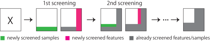
Figure 1: Schematic illustration of the proposed approach. By iterating safe feature screening and safe sample screening, irrelevant features and samples are safely removed out from the training set. A significant advantage of considering them simultaneously rather than individually is that they have a synergy effect in the sense that the screening performances (the number of features/samples that can be safely removed out) are gradually improved by exploiting the results in earlier steps.

These findings suggest that, safe screening performances of features and samples can be both improved by alternatively repeating them. Figure 1 is a schematic illustration of the simultaneous safe screening approach.

Another interesting finding we first introduce in this paper is that, by simultaneously considering regions both in the dual and the primal spaces, we can also identify features and samples that are guaranteed to be active. We call this technique as safe keeping. While safe screening assures no false negative findings, safe keeping guarantees no false positive findings of active features/samples. By combining these two techniques, we can better identify active features/samples. A practical advantage of safe keeping is that we do not have to consider the safe screening rules anymore for features and samples which are identified as active by safe keeping. This is helpful for reducing the computational costs of safe screening rule evaluations especially in the context of dynamic safe screening [8].

1.1 Notation and outline

We use the following notations in the rest of the paper. For any natural number $n$, we define $[n]:=\{1,\ldots,n\}$. For an $n\times d$ matrix $M$, its $i$-th row and $j$-th column are denoted as $M_{i:}$ and $M_{:j}$, respectively, for $i\in[n]$ and $j\in[d]$. The $L_{1}$ norm, the $L_{2}$ norm and the $L_{\infty}$ norm of a vector $v\in\mathbb{R}^{m}$ are respectively written as $\|v\|_{1}:=\sum_{k\in[m]}|v_{k}|$, $\|v\|_{2}:=\sqrt{\sum_{k\in[m]}|v_{k}|^{2}}$ and $\|v\|_{\infty}:=\max_{k\in[m]}|v_{k}|$. For a scalar $z$, we define $[z]_{+}:=\max\{0,z\}$. We write the subdifferential operator as $\partial$, and remind that the subdifferential of $L_{1}$ norm is given as $\partial\|v\|_{1}=\{g\mid\|g\|_{\infty}\leq 1,g^{\top}v=\|v\|_{1}\}$. For a function $f$, we denote its domain as ${\rm dom}f$.

Here is the outline of the paper. §2 introduces the problem formulation we mainly consider in this paper and basic concepts of safe screening. §3 describes our main contribution where we show that simultaneously screening features and samples has synergetic advantages. §4 also presents another contribution where we introduce a new approach for predicting active set without false positive errors. §5 discusses another problem that induces spasities both in features and samples. §6 covers numerical experiments for demonstrating the advantage of the simultaneous safe screening. §7 concludes the paper.

2 Preliminaries

In this section, we first describe the problem formulation in §2.1. Then, we briefly summarize the basic concepts of safe feature screening and safe sample screening in §2.2 and §2.3, respectively.

2.1 Problem formulation

Consider classification and regression problems with the number of samples $n$ and the number of features $d$. The training set is written as $\{(x_{i},y_{i})\}_{i\in[n]}$ where $x_{i}\in\mathbb{R}^{d}$, and $y_{i}\in\{-1,1\}$ for classification and $y_{i}\in\mathbb{R}$ for regression. The $n\times d$ input data matrix (design matrix) is denoted as $X:=[x_{1},\ldots,x_{n}]^{\top}$.

We consider a linear classification and regression function in the form of $f(x)=x^{\top}w$, and study the problem of estimating the parameter $w\in\mathbb{R}^{d}$ by solving a class of regularized empirical risk minimization problems:

$$\min_{w\in\mathbb{R}^{d}}P_{\lambda}(w):=\lambda\psi(w)+\frac{1}{n}\sum_{i\in[n]}\ell_{i}(x_{i}^{\top}w),$$ (1)

where $\psi$ is a penalty function, $\ell_{i}$ is a loss function for the $i$-th sample, and $\lambda>0$ is a trade-off parameter for controlling the balance between the penalty and the loss.

In this paper, we study doubly sparse modeling, i.e., a pair of penalty and loss function that induces sparsities both in features and samples. As specific working examples, we consider $L_{1}$-penalized smoothed hinge SV classification and $L_{1}$-penalized smoothed $\varepsilon$-insensitive SV regression. The use of these smoothed loss functions are known to produce almost same solutions as the original hinge or $\varepsilon$-insensitive loss functions [17]. We will discuss other doubly sparse modeling problem in §5.

Remembering that the original SVMs are trained with $L_{2}$ penalty, by combining an additional $L_{1}$-penalty, our penalty function $\psi$ is written as elastic net penalty:

$$\psi(w):=\|w\|_{1}+\frac{\beta}{2}\|w\|_{2}^{2},$$ (2)

where $\beta>0$ is a balancing parameter which we omit hereafter by substituting $\beta=1$ for notational simplicity. The smoothed hinge loss and the smoothed $\varepsilon$-insensitive loss are respectively written as

$$\!\!\ell_{i}(x_{i}^{\top}w)\!\! :=\!\!\begin{cases}0&(y_{i}x_{i}^{\top}w>1),\\ 1-y_{i}x_{i}^{\top}w-\frac{\gamma}{2}&(y_{i}x_{i}^{\top}w<1-\gamma),\\ \frac{1}{2\gamma}(1-y_{i}x_{i}^{\top}w)^{2}&({\rm otherwise}),\end{cases}$$ (3)

$$\!\!\ell_{i}(x_{i}^{\top}w)\!\! :=\!\!\begin{cases}\!0&\!\!\!\!(|x_{i}^{\top}w-y_{i}|\!\!<\!\!\varepsilon),\\ \!|x_{i}^{\top}\!w\!-\!y_{i}|\!\!-\!\varepsilon\!-\!\frac{\gamma}{2}&\!\!\!\!\!(|x_{i}^{\top}w\!-\!y_{i}|\!\!>\!\!\varepsilon\!\!+\!\!\gamma),\\ \!\frac{1}{2\gamma}(|x_{i}^{\top}w-y_{i}|\!\!-\varepsilon)^{2}&\!\!\!\!\!({\rm otherwise}),\end{cases}$$ (4)

where $\gamma>0$ is a tuning parameter. There are profiles the smoothed hinge loss and the smoothed $\varepsilon$-insensitive loss as shown in Figure 2.

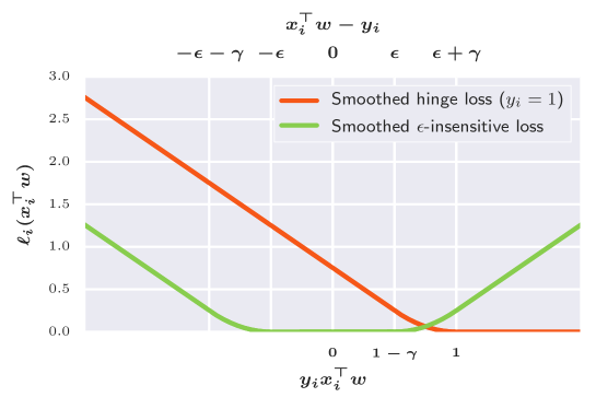
Figure 2: Illustrations of the smoothed hinge loss (orange) and the smoothed $\varepsilon$-insensitive loss (green), where $\gamma=0.5$ and $\varepsilon=0.5$.

Using Fenchel’s duality theorem (see, e.g., Corollary 31.2.1 in [18]), the dual problem of (1) is written as

$$\!\!\!\!\!\max_{\alpha}D_{\lambda}(\alpha):=-\lambda\psi^{*}\!\!\left(\frac{1}{\lambda n}X^{\top}\alpha\right)\!\!-\frac{1}{n}\!\sum_{i\in[n]}\!\ell_{i}^{*}(-\alpha_{i}),$$ (5)

where $\psi^{*}$ and $\ell^{*}$ is convex conjugate function of $\psi$ and $\ell$, respectively. The convex conjugate function of the penalty term in (2) is given as (see [17] )

$$\psi^{*}(v) =\frac{1}{2}\sum_{j=1}^{d}([|v_{j}|-1]_{+})^{2}.$$

The convex conjugate functions of the smoothed hinge loss and the smoothed $\varepsilon$-insensitive loss are respectively written as

$$\ell^{*}_{i}(\alpha_{i}) =\begin{cases}\frac{\gamma}{2}\alpha_{i}^{2}+y_{i}\alpha_{i}&(y_{i}\alpha_{i}\in[-1,0]),\\ \infty&({\rm otherwise}),\end{cases}$$ (6)

and

$$\ell^{*}_{i}(\alpha_{i}) =\begin{cases}\frac{\gamma}{2}\alpha_{i}^{2}+y_{i}\alpha_{i}+\varepsilon|\alpha_{i}|&(\alpha_{i}\in[-1,1]),\\ \infty&({\rm otherwise}).\end{cases}$$ (7)

We call the problems in (1) and (5) as primal problem and dual problem, respectively, and denote the primal optimal solution as $w^{*}\in\mathbb{R}^{d}$ and the dual optimal solution as $\alpha^{*}\in\mathbb{R}^{n}$.

2.2 Safe feature screening

The goal of safe feature screening is to identify a part of non-active features $\{j\in[d]\mid w_{j}^{*}=0\}$ before or during the optimization process. Safe feature screening is built on the following KKT optimality condition (see Theorem 31.3 in [18])

$$\frac{1}{\lambda n}X^{\top}\alpha^{*} \in\partial\psi(w^{*}).$$ (8)

In the case of our specific regularization term (2), the optimality condition (8) is written as

$$\frac{1}{\lambda n}X_{:j}^{\top}\alpha^{*}\in\begin{cases}\cfrac{w^{*}_{j}}{|w^{*}_{j}|}+w^{*}_{j}&(w^{*}_{j}\neq 0),\\ [-1,1]&(w^{*}_{j}=0).\end{cases}$$ (9)

The optimality condition (9) indicates that

$$|X_{:j}^{\top}\alpha^{*}|\leq\lambda n~{}\Rightarrow~{}w^{*}_{j}=0.$$

The basic idea behind safe feature screening is to construct a region $\Theta_{\alpha^{*}}\subset\mathbb{R}^{n}$ in the dual space so that $\alpha^{*}\in\Theta_{\alpha^{*}}$, and then compute an upper bound $UB(|X_{:j}^{\top}\alpha^{*}|):=\max_{\alpha\in\Theta_{\alpha^{*}}}|X_{:j}^{\top}\alpha|$. Using this upper bound, we can construct a safe feature screening rule in the form of

$$UB(|X_{:j}^{\top}\alpha^{*}|)\leq\lambda n~{}\Rightarrow~{}w_{j}^{*}=0.$$

After the seminal work [5], many different approaches for constructing a region $\Theta_{\alpha^{*}}$ have been developed (see §1). Among those, we use an approach in [13]. Noting the fact that the convex conjugate function $\ell^{*}$ is $\gamma$-strongly convex, and henceforth the dual objective function $D_{\lambda}(\alpha)$ is $\gamma/n$-strongly concave, we can define a region

$$\Theta_{\alpha^{*}}:=\{\alpha\mid\|\hat{\alpha}-\alpha\|_{2}\leq\sqrt{2nG_{\lambda}(\hat{w},\hat{\alpha})/\gamma}\},$$ (10)

where $G_{\lambda}(\hat{w},\hat{\alpha}):=P_{\lambda}(\hat{w})-D_{\lambda}(\hat{w})$ is the duality gap defined by an arbitrary pair of primal feasible solution $\hat{w}\in{\rm dom}P_{\lambda}$ and dual feasible solution $\hat{\alpha}\in{\rm dom}D_{\lambda}$. Since the region $\Theta_{\alpha^{*}}$ is a sphere, we can explicitly write the upper bound as

$$\!\!UB(|X_{:j}^{\top}\alpha^{*}|)\!=\!|X_{:j}^{\top}\hat{\alpha}|\!+\!\|X_{:j}\|_{2}\sqrt{2nG_{\lambda}(\hat{w},\hat{\alpha})/\gamma}.$$ (11)

2.3 Safe sample screening

The goal of safe sample screening is to identify a part of non-active samples $\{i\in[n]\mid\alpha_{i}^{*}=0,\pm 1\}$ before or during the optimization process. Here, we slightly abuse the word “non-active” in the sense that we call a sample to be non-active not only when the corresponding $\alpha^{*}_{i}$ is $0$, but also when it is $\pm 1$. Although the $i$-th sample can be removed out only when $\alpha^{*}_{i}=0$, we have similar computational advantages when we can guarantee that $\alpha^{*}_{i}=\pm 1$ because the size of the optimization problem can be reduced.

Safe sample screening is also built on the KKT optimality condition

$$x_{i}^{\top}w^{*} \in\partial\ell_{i}^{*}(-\alpha^{*}_{i}).$$ (12)

In the case of smoothed hinge loss, the KKT condition (12) is written when $y_{i}=1$ as

$$x_{i}^{\top}w^{*}\in\begin{cases}[1,\infty)&(\alpha^{*}_{i}=0)\\ (-\infty,1-\gamma]&(\alpha^{*}_{i}=1)\\ -\gamma\alpha_{i}^{*}+1&(\alpha^{*}_{i}\in(0,1)).\end{cases}$$ (13)

We construct a region $\Theta_{w^{*}}\subset\mathbb{R}^{d}$ in the primal space so that $w^{*}\in\Theta_{w^{*}}$, and then compute a lower bound $LB(x_{i}^{\top}w^{*}):=\min_{w\in\Theta_{w^{*}}}x_{i}^{\top}w$ and an upper bound $UB(x_{i}^{\top}w^{*}):=\max_{w\in\Theta_{w^{*}}}x_{i}^{\top}w$. The optimality condition (13) suggests that

$$LB(x_{i}^{\top}w^{*})\geq 1~{}\Rightarrow~{}\alpha_{i}^{*}=0,$$

$$UB(x_{i}^{\top}w^{*})\leq 1-\gamma~{}\Rightarrow~{}\alpha_{i}^{*}=1.$$

Similarly, for $y_{i}=-1$, the optimality condition is written as

$$x_{i}^{\top}w^{*}\in\begin{cases}(-\infty,-1]&(\alpha^{*}_{i}=0)\\ [\gamma-1,\infty)&(\alpha^{*}_{i}=-1)\\ -\gamma\alpha^{*}_{i}-1&(\alpha^{*}_{i}\in(-1,0)),\end{cases}$$ (14)

suggesting that

$$UB(y_{i}x_{i}^{\top}w^{*})\leq-1~{}\Rightarrow~{}\alpha_{i}^{*}=0,$$

$$LB(y_{i}x_{i}^{\top}w^{*})\geq\gamma-1~{}\Rightarrow~{}\alpha_{i}^{*}=-1.$$

In the case of smoothed $\varepsilon$-insensitive loss, the optimality condition (12) is written as

$$x_{i}^{\top}w^{*}\in\begin{cases}[y_{i}-\varepsilon,y_{i}+\varepsilon]&(\alpha^{*}_{i}=0),\\ [\gamma+y_{i}+\varepsilon,\infty)&(\alpha^{*}_{i}=-1),\\ (-\infty,-\gamma+y_{i}-\varepsilon]&(\alpha^{*}_{i}=1),\\ -\gamma\alpha^{*}_{i}+y_{i}+\varepsilon&(\alpha^{*}_{i}\in(-1,0)),\\ -\gamma\alpha^{*}_{i}+y_{i}-\varepsilon&(\alpha^{*}_{i}\in(0,1)).\end{cases}$$ (15)

It indicates that

$$LB(x_{i}^{\top}w^{*})\geq y_{i}-\varepsilon~{}\text{ and }~{}UB(x_{i}^{\top}w^{*})\leq y_{i}+\varepsilon~{}\Rightarrow~{}\alpha_{i}^{*}=0,$$

$$LB(x_{i}^{\top}w^{*})\geq\gamma+y_{i}+\varepsilon~{}\Rightarrow~{}\alpha_{i}^{*}=-1,$$

$$UB(x_{i}^{\top}w^{*})\leq-\gamma+y_{i}-\varepsilon~{}\Rightarrow~{}\alpha_{i}^{*}=1.$$

In order to develop a sphere region $\Theta_{w^{*}}$ in the primal space, we extend the duality GAP-based safe feature screening approach proposed in [13] into safe sample screening context. The result is summarized in the following lemma.

Lemma 1.

For any $\hat{w}\in{\rm dom}P_{\lambda}$ and $\hat{\alpha}\in{\rm dom}D_{\lambda}$,

$$w^{*}\in\Theta_{w^{*}}=\{w\mid\|\hat{w}-w\|_{2}\leq\sqrt{2G_{\lambda}(\hat{w},\hat{\alpha})/\lambda}\},$$ (16)

Furthermore, using the sphere form region $\Theta_{w^{*}}$ in (16), for any $\hat{w}\in{\rm dom}P_{\lambda}$ and $\hat{\alpha}\in{\rm dom}D_{\lambda}$, a pair of lower and upper bounds of $x_{i}^{\top}w^{*}$ are given as

$$LB(x_{i}^{\top}w^{*}) =x_{i}^{\top}\hat{w}-\|x_{i}\|_{2}\sqrt{2G_{\lambda}(\hat{w},\hat{\alpha})/\lambda},$$ (17a)

$$UB(x_{i}^{\top}w^{*}) =x_{i}^{\top}\hat{w}+\|x_{i}\|_{2}\sqrt{2G_{\lambda}(\hat{w},\hat{\alpha})/\lambda}.$$ (17b)

The proof of Lemma 1 is presented in Appendix A.

3 Simultaneous safe screening

We have shown that, for doubly sparse modeling problems, safe screening rules for both of features and samples can be constructed respectively. This has not been explored in depth regardless of its practical importance. In this paper we further develop the framework in which safe feature screening and safe sample screening are alternately iterated. A significant additional benefit of this framework is that the result of the previous safe feature screening can be exploited for making the primal region $\Theta_{w^{*}}$ smaller, meaning that the performance of the next safe sample screening can be improved, and vice-versa.

The following two theorems formally state these ideas. First, Theorem 2 states that we can obtain tighter upper bound for feature screening by exploiting the result of the previous safe sample screening.

Theorem 2.

Consider a safe feature screening problem given arbitrary pair of primal and dual feasible solution $\hat{w}\in{\rm dom}P_{\lambda}$ and $\hat{\alpha}\in{\rm dom}D_{\lambda}$. Furthermore, suppose that the result of the previous safe sample screening step assures the optimal values $\alpha_{i}^{*}$ for a subset of the samples $i\in{\cal S}\subset[n]$. Let ${\cal U}_{s}:=[n]\setminus{\cal S}$, $r_{D}:=\sqrt{2nG_{\lambda}(\hat{w},\hat{\alpha})/\gamma}$, and $\tilde{\alpha}$ be an $n$-dimensional vector whose element is defined as $\tilde{\alpha}_{i}=\hat{\alpha}_{i}$ for $i\in{\cal U}_{s}$ and $\tilde{\alpha}_{i}=\alpha^{*}_{i}$ for $i\in{\cal S}$. Then, $|X_{:j}^{\top}\alpha^{*}|$ is bounded from above by the following upper bound:

$$\!\!\!\!\!\!\tilde{UB}(\!|X_{:j}^{\top}\alpha^{*}|\!)\!\!:=\!\!|X_{:j}^{\top}\tilde{\alpha}|\!+\!\|X_{:j{\cal U}_{s}}\|_{2}\sqrt{r_{D}^{2}\!\!-\!\!\|\hat{\alpha}_{{\cal S}}\!-\!\alpha^{*}_{{\cal S}}\|_{2}^{2}},$$ (18)

and the upper bound in (18) is tighter than or equal to that in (11), i.e., $\tilde{UB}(|X_{:j}^{\top}\alpha^{*}|)\leq UB(|X_{:j}^{\top}\alpha^{*}|)$.

The proof of Theorem 2 is presented in Appendix. By replacing the upper bounds in (11) with that in (18) in the safe feature screening step, there are more chance for screening out non-active features.

Next, Theorem 3 states that we can obtain tighter lower and upper bounds for sample screening by exploiting the result of the previous safe feature screening.

Theorem 3.

Consider a safe sample screening problem given arbitrary pair of primal and dual feasible solutions $\hat{w}\in{\rm dom}P_{\lambda}$ and $\hat{\alpha}\in{\rm dom}D_{\lambda}$. Furthermore, suppose that the result of the previous safe feature screening step assures that $w_{j}^{*}=0$ for a subset of the features $j\in{\cal F}\subset[d]$. Let ${\cal U}_{f}:=[d]\setminus{\cal F}$, $r_{P}:=\sqrt{2G_{\lambda}(\hat{w},\hat{\alpha})/\lambda}$, and $\tilde{w}$ be a $d$-dimensional vector whose element is defined as $\tilde{w}_{j}=\hat{w}_{j}$ for $j\in{\cal U}_{f}$ and $\tilde{w}_{j}=0$ for $j\in{\cal F}$. Then, $x_{i}^{\top}w^{*}$ is bounded from below and above respectively by the following lower and upper bounds:

$$\tilde{LB}(x_{i}^{\top}w^{*}) :=x_{i}^{\top}\tilde{w}-\|x_{i{\cal U}_{f}}\|_{2}\sqrt{r_{P}^{2}-\|\hat{w}_{{\cal F}}\|_{2}^{2}}$$ (19a)

$$\tilde{UB}(x_{i}^{\top}w^{*}) :=x_{i}^{\top}\tilde{w}+\|x_{i{\cal U}_{f}}\|_{2}\sqrt{r_{P}^{2}-\|\hat{w}_{{\cal F}}\|_{2}^{2}}$$ (19b)

and these bounds in (19) are tighter than or equal to those in (17), i.e., $\tilde{LB}(x_{i}^{\top}w^{*})\geq LB(x_{i}^{\top}w^{*})$ and $\tilde{UB}(x_{i}^{\top}w^{*})\leq UB(x_{i}^{\top}w^{*})$.

The proof of Theorem 3 is presented in Appendix. By replacing the lower and the upper bounds in (17) with those in (19) in the safe sample screening step, there are more chance to be able to screen out non-active samples. Again, we note that the tighter bounds in (19) are different from the bounds that would be obtained just by using $\tilde{w}$ as the primal feasible solution $\hat{w}$ in (11).

Theorems 2 and 3 suggests that, by alternately iterating feature screening and sample screening, more and more features and samples could be screened out. This iteration process can be terminated when there are few chances to be able to screen out additional features and samples. Such a termination condition can be developed by using the results in the next section.

4 Safe keeping of active features and samples

Safe screening studies initiated by the seminal work by [5] enabled us to identify a part of non-active features/samples before actually solving the optimization problem. In other words, safe screening is interpreted as an active set prediction method without false negative error (an error that truly active features/samples are predicted as non-active). In this section, we show that, by exploiting the two regions in the dual and the primal spaces, we can develop an active set prediction method without false positive error (an error that truly non-active features/samples are predicted as active). We call the latter approach as safe feature/sample keeping.

Safe feature keeping rule can be constructed by using the region in the primal space. Using $\Theta_{w^{*}}$ in (16), we can get the lower bound of $|w_{j}^{*}|$ for $j\in[d]$ as $LB(|w_{j}^{*}|):=|\hat{w}_{j}|-\sqrt{2G_{\lambda}(\hat{w},\hat{\alpha})}$. Using this lower bound, safe feature keeping rule is simply formulated as the following theorem.

Theorem 4.

For an arbitrary pair of primal feasible solution $\hat{w}\in{\rm dom}P_{\lambda}$ and dual feasible solution $\hat{\alpha}\in{\rm dom}D_{\lambda}$,

$$|\hat{w}_{j}|-\sqrt{2G_{\lambda}(\hat{w},\hat{\alpha})}>0~{}\Rightarrow~{}w_{j}^{*}\neq 0~{}{\text{for}}~{}j\in[d].$$

Similarly, safe sample keeping rule can be constructed by using a region in the dual space. The condition for $\alpha_{i}^{*}$ being active is written as $\alpha_{i}^{*}\neq-1,0,1$. This can be guaranteed when the condition $\alpha^{*}_{i}\in(0,1)$ or $\alpha^{*}_{i}\in(-1,0)$ holds for the $i$-th element of $\forall\alpha\in\Theta_{\alpha^{*}}$. Since $\Theta_{\alpha^{*}}$ is a sphere, safe sample keeping rule can be simply derived by (10).

Theorem 5.

For an arbitrary pair of primal feasible solution $\hat{w}\in{\rm dom}P_{\lambda}$ and dual feasible solutionx $\hat{\alpha}\in{\rm dom}D_{\lambda}$,

$$|\hat{\alpha}_{i}|\!\!-\!\!\sqrt{2nG_{\lambda}(\hat{w},\hat{\alpha})/\gamma}>0\text{ and }|\hat{\alpha}_{i}|\!\!+\!\!\sqrt{2nG_{\lambda}(\hat{w},\hat{\alpha})/\gamma}\!<\!1\Rightarrow\alpha_{i}^{*}\neq 0,\pm 1\text{ for }i\in[n].$$

When we use safe screening approaches, there is a trade-off between the computational costs of evaluating safe screening rules and the computational time saving by screening out some features/samples. If we know in advance that some of the features/samples cannot be non-active by using safe keeping approaches, we do not have to waste the rule evaluation costs for those features/samples. Safe screening rule evaluation costs would be more significant in dynamic screening and our simultaneous screening scenarios because rules are repeatedly evaluated. By combining safe screening and safe keeping approaches, we can get an information about how many features/samples are not yet determined to be active or non-active. This information can be also used as a stopping criteria of dynamic screening and our simultaneous screening. We can stop evaluating safe screening rules when there only remain few features/samples that have not been determined to be active or non-active. Specifically, if the fraction of the sum of the safely screened features/samples and the safely kept features/samples is close to one, then we have few chances to be able to safely screen out additional features/samples. The additional computational complexities of safe feature/sample keeping for a single feature/sample is ${\cal O}(1)$, which is negligible compared with ${\cal O}(n)$ complexity for safe feature screening and ${\cal O}(d)$ complexity for safe sample screening.

We finally note that, in our particular working problem of $L_{1}$ smooth SVC and $L_{1}$ smooth SVR, safe keeping is also possible by using the KKT optimality conditions in (9) for features, and (13) - (15) for samples. We describe the details in the Appendix.

5 LP-based simultaneous safe screening

In this section, we consider another empirical risk minimization problem that induces sparsities both in features and samples. Specifically, we study a problem with $L_{1}$-penalty $\psi(w)=\|w\|_{1}$ and vanilla hinge loss $\ell_{i}(w)=\max\{0,1-y_{i}x_{i}^{\top}w\}$, which we call LP-based SVM because it is casted into a linear program (LP). LP-based SVM has been studied in [19, 20], and also in boosting context. LPBoost [21] solves LP-based SVM via the column generation approach of linear programming. while ERLPBoost [22] is a variant of LPBoost obtained by adding a small entropic term in the LP objective. Sparse LPBoost [23] is simiilar to simultaneous screening in that it iteratively solves LP sub-problems for features and samples. LP-based SVM induces feature sparsity due to $L_{1}$-penalty and sample sparsity due to the property of hinge loss.

The convex conjugate functions of $L_{1}$-penalty and vanilla hinge loss are respectively written as

$$\psi^{*}\left(v\right) :=\begin{cases}0&(\|v\|_{\infty}\leq 1),\\ \infty&(\text{otherwise}),\end{cases}$$ (20)

$$\ell^{*}_{i}(\alpha_{i}) :=\begin{cases}y_{i}\alpha_{i}&y_{i}\alpha_{i}\in[-1,0],\\ \infty&(\text{otherwise}),\end{cases}$$ (21)

and the dual problem is written as

$$\max_{\alpha}D_{\lambda}(\alpha):=\max_{\alpha}\left\{y^{\top}\alpha\right\}~{}{\text{s.t.}}~{}\left\|\frac{1}{\lambda n}\alpha_{i}x_{i}\right\|_{\infty}\leq 1,~{}y_{i}\alpha_{i}\in[0,1]~{}~{}\forall i\in[n].$$

5.1 Safe feature screening for LP-based SVM

Feature safe screening for LP-based SVM was studied in the seminal safe feature screening paper by [5]. However, the method presented in their paper requires a precise optimal solution of an LP-based SVM with a different penalty parameter $\lambda$. This requirement is impractical because precise optimal solutions are often difficult to get numerically as recently pointed out by [12]. Here, we present a novel safe feature screening method for LP-based SVM that only requires an arbitrary pair of a primal feasible solution $\hat{w}\in{\rm dom}P_{\lambda}$ and a dual feasible solution $\hat{\alpha}\in{\rm dom}D_{\lambda}$. The proposed safe feature screening method for LP-based SVM is summarized in the following theorem.

Theorem 6.

Consider safe feature screening problem given an arbitrary pair of a primal feasible solution $\hat{w}\in{\rm dom}P_{\lambda}$ and a dual feasible solution $\hat{\alpha}\in{\rm dom}D_{\lambda}$. Let $\ell_{q}:=\lfloor y^{\top}\hat{\alpha}\rfloor$, $u_{q}=\lfloor P_{\lambda}(\hat{w})\rfloor$, $Z:=[y_{1}x_{1},\ldots,y_{n}x_{n}]^{\top}\in\mathbb{R}^{n\times d}$, and $Z_{:j}^{\prime}\in\mathbb{R}^{n}$, $j\in[d]$, be the vector obtained by sorting $Z_{:j}$ in increasing order. Furthermore, let $n_{Z_{:j}^{\prime}}$ and $p_{Z_{:j}^{\prime}}$ represent the numbers of negative and positive elements of $Z_{:j}^{\prime}$, respectively. Then,

$$LB(X_{:j}^{\top}\alpha^{*})<-\lambda n~{}\text{and}~{}UB(X_{:j}^{\top}\alpha^{*})>\lambda n~{}\Rightarrow~{}w_{j}^{*}=0,$$

where

$$LB(X_{:j}^{\top}\alpha^{*}):=\begin{cases}\sum_{i=1}^{l_{q}}Z^{\prime}_{ij}+(y^{\top}\hat{\alpha}-l_{q})Z^{\prime}_{(l_{q}+1)j}&(n_{Z^{\prime}_{:j}}<l_{q}+1),\\ \sum_{i=1}^{u_{q}}Z^{\prime}_{ij}+(P_{\lambda}(\hat{w})-u_{q}),Z^{\prime}_{u_{q}j}&(n_{Z^{\prime}_{:j}}>u_{q})\\ \sum_{i=1}^{n}\min\{0,Z^{\prime}_{ij}\}&({\rm otherwise}),\end{cases}$$

$$UB(X_{:j}^{\top}\alpha^{*}):=\begin{cases}\!\sum_{i=n-l_{q}}^{n}\!\!Z^{\prime}_{ij}+(y^{\top}\hat{\alpha}-l_{q})Z^{\prime}_{(n-l_{q}-1)j}&\!\!\!\!\!\!(p_{Z^{\prime}_{:j}}<l_{q}+1),\\ \!\sum_{i=n-u_{q}}^{n}\!\!Z^{\prime}_{ij}+(P_{\lambda}(\hat{w})-u_{q})Z^{\prime}_{(n-u_{q}-1)j}&\!\!\!\!\!\!(p_{Z^{\prime}_{:j}}>u_{q}),\\ \!\sum_{i=1}^{n}\max\{0,Z^{\prime}_{ij}\}&\!\!\!\!\!\!({\rm otherwise}).\end{cases}$$

The proof of Theorem 6 is presented in Appendix.

5.2 Safe sample screening for LP-based SVM

Here, we develop a novel safe sample screening method for LP-based SVM as summarized in the following theorem.

Theorem 7.

Consider safe sample screening given an arbitrary primal feasible solution $\hat{w}\in{\rm dom}P_{\lambda}$. Let $g_{\ell_{i}}(w)$ be a subgradient of vanilla hinge loss $\ell_{i}(w)$ for $w\in{\rm dom}P_{\lambda}$, and define $k:=\lambda\|\hat{w}\|_{1}+\frac{1}{n}\sum_{i\in[n]}g_{\ell_{i}(\hat{w})}^{\top}\hat{w}$. Then,

$$y_{i}=+1\text{ and }LB(x_{i}^{\top}w^{*})>+1~{}\Rightarrow~{}\alpha_{i}^{*}=+1,$$

$$y_{i}=+1\text{ and }UB(x_{i}^{\top}w^{*})<+1~{}\Rightarrow~{}\alpha_{i}^{*}=0,$$

$$y_{i}=-1\text{ and }LB(x_{i}^{\top}w^{*})>-1~{}\Rightarrow~{}\alpha_{i}^{*}=0,$$

$$y_{i}=-1\text{ and }UB(x_{i}^{\top}w^{*})<-1~{}\Rightarrow~{}\alpha_{i}^{*}=-1,$$

where

$$LB(x_{i}^{\top}\!w^{*})\!\!:=\!\!\max_{\mu>0}\{\mu k\}~{}{\rm{s.t.}}\left\|\!\!-\frac{1}{\lambda}x_{i}-\frac{\mu}{\lambda n}\sum_{i=1}^{n}g_{\ell_{i}}(\hat{w})\right\|_{\infty}\leq\mu,$$

$$UB(x_{i}^{\top}\!w^{*})\!\!:=\!\!\max_{\mu>0}\{\mu k\}~{}{\rm{s.t.}}\left\|\!\!\!\!\phantom{-}\frac{1}{\lambda}x_{i}-\frac{\mu}{\lambda n}\sum_{i=1}^{n}g_{\ell_{i}}(\hat{w})\right\|_{\infty}\leq\mu.$$

The proof of Theorem 7 is presented in Appendix. Although the lower and the upper bounds are not explicitly presented, these optimization problems can be easily solved because they are just linear programs with one variable $\mu>0$.

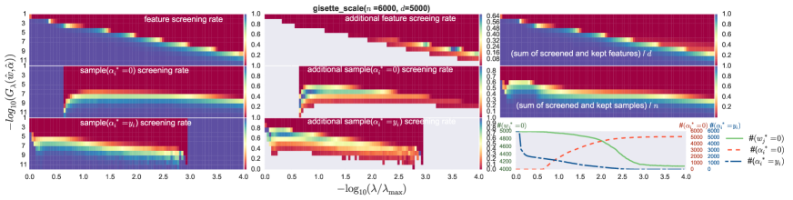
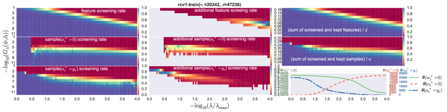
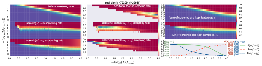
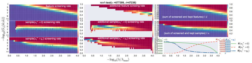
Figure 3: Safe screening and keeping rates for classification problems (for real-sim and rcv1-test datasets). The three plots in the left show the individual safe feature/sample screening rates (the middle and the bottom ones are for $\alpha_{i}^{*}=0$ and $\alpha_{i}^{*}=\pm 1$, respectively). The three plots in the center show the additional safe screening rates by simultaneously considering feature and sample screenings. The gray area in these center plots corresponds to the blue area in the corresponding left plot. In these gray area, the individual safe screening performances are good enough (screening rate $>0.95$) and additional screening is unnecessary. The top right and middle right plots show the safe keeping rates for feature and samples, respectively. The bottom right plot shows the numbers of active features and samples for various values of $\lambda$.

As we discussed in §3, by alternatively iterating safe feature screening in §5.1 and safe sample screening in §5.2, we can make the regions in the dual and the primal regions step by step, indicating that the chance of screening out more features and samples increases .

6 Numerical experiments

We demonstrate the advantage of simultaneous safe screening through numerical experiments. After we describe the experimental setups in §6.1, we report the results on safe screening and keeping rates, and computation time savings in §6.2 and §6.2, respectively.

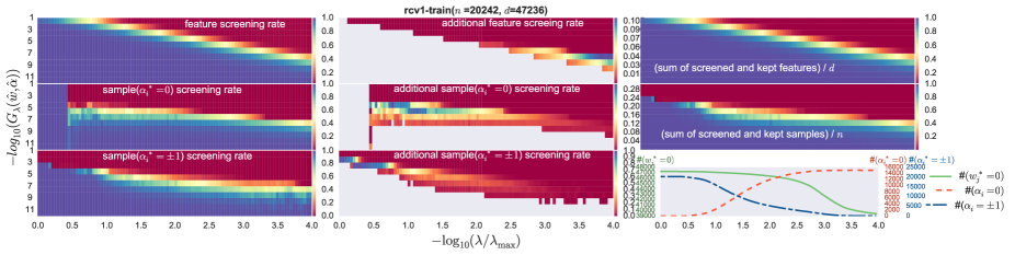
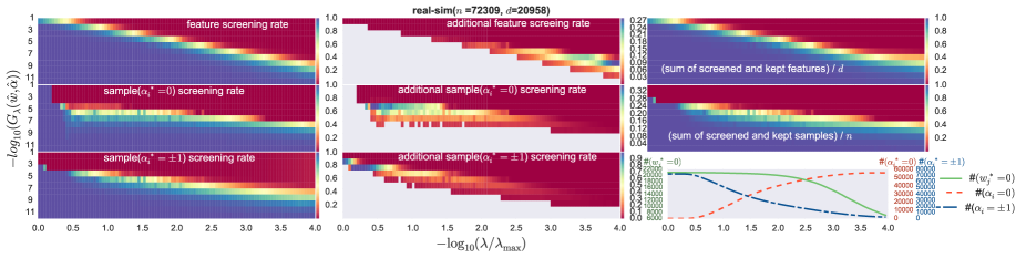
Figure 4: Safe screening and keeping rates in regression problems. See the caption in Figure 3.

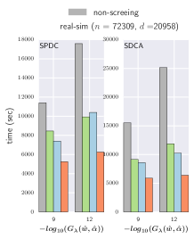
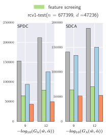
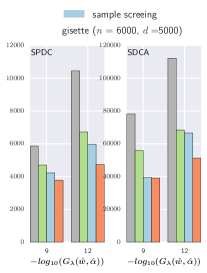
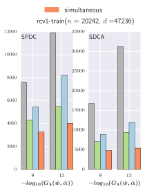
Figure 5: Total computation time for training 100 solutions for various values of $\lambda$ in classification problems.

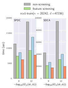
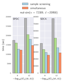
Figure 6: Total computation time for training 100 solutions for various values of $\lambda$ in regression problems.

6.1 Experimental setups

Table 1 summarizes the datasets used in the experiments. We picked up four datasets whose numbers of features and samples are both large from libsvm dataset repository [4]. These are all classification datasets. For regression experiments, we just used the label indicator variables as scalar response variables.

Table 1: Benchmark datasets used in the experiments.

dataset name	sample size: $n$	feature size: $d$	#(nnz)/$nd$
real-sim	72,309	20,958	0.002448
rcv1-test	677,399	47,236	0.025639
gisette	6,000	5,000	0.991000
rcv1-train	20,242	47,236	0.001568

#(nnz) indicates the number of non-zero elements.

Here, we report the results on $L_{1}$-penalized smoothed hinge SV classification and $L_{1}$-penalized smoothed $\varepsilon$-insensitive SV regression. We set $\lambda_{\max}:=\|Z^{\top}\bm{1}\|_{\infty}$ for classification and $\lambda_{\max}:=\|X^{\top}\bm{1}\|_{\infty}$ for regression, and considered problems with various values of the penalty parameter $\lambda$ between $\lambda_{\max}$ and $10^{-4}\lambda_{\max}$. The parameter in the smoothed hinge loss $\gamma$ is set to be $0.5$. Also, the parameters in the smoothed $\varepsilon$-insensitive loss $\gamma$ is set to be $0.1$ and $\varepsilon$ is set to be $0.5$. The proposed methods can be used with any optimization solvers as long as they provide both primal and dual sequences of solutions that converge to the optimal solution. For the experiments, we used Proximal Stochastic Dual Coordinate Ascent (SDCA) [17] and Stochastic Primal-Dual Coordinate (SPDC) [24] because they are state-of-the-art optimization methods for general large-scale regularized empirical risk minimization problems. We wrote the code in C++ along with Eigen library for some numerical computations. The code is provided as a supplementary material, and will be put in public domain after the paper is accepted. All the computations were conducted by using a single core of an Intel Xeon CPU E5-2643 v2 (3.50GHz), 64GB MEM.

6.2 Safe screening and keeping rates

For demonstrating the synergy effect of simultaneous safe screening, we compared the simultaneous screening rates with individual safe screening rates. Figures 3 and 4 shows the results on classification and regression problems,respectively. In the $3\times 3$ subplots, the letf plots indicate the individual screening rates defined as (#(screened features or samples) / #($w^{*}_{j}=0$ or $\alpha^{*}_{i}=0$ or $\alpha^{*}_{i}=\pm 1$)). The center plots indicate the additional screening rates by the synergy effect defined as (#(additionally screened features or samples) / #($w^{*}_{j}=0$ or $\alpha^{*}_{i}=0$ or $\alpha^{*}_{i}=\pm 1$)). The top plots represent the results on feature screening, while the middle and the bottom plots show the results on sample screening (for each of $\alpha^{*}_{i}=0$ and $\alpha_{i}^{*}=\pm 1$). We investigated the screening rates for various values of $\lambda$ in the horizontal axis and for various quality of the solutions measured in terms of the duality gap in the vertical axis. In all the datasets, we observed that it is valuable to consider both feature and sample screening when the numbers of features and samples are both large. In addition, we confirmed that there are improvements in screening rates by the synergy effect both in feature and sample screenings especially when duality gap $G_{\lambda}(\hat{w},\hat{\alpha})$ is large. Note that gray areas in the center plots corresponds to the blue area in the corresponding left plot, where the individual safe screening performances are good enough (screening rate $>0.95$) and additional screening is unnecessary.

The top left and the middle left plots show the rates of features and samples, respectively, that are determined to be active or non-active by using safe keeping and safe screening approaches, respectively. We see that, by combining safe keeping and safe screening approaches, a large portion of features/samples can be determined to be active or non-active without actually solving the optimization problems. The bottom right plot shows the number of non-active features/samples for various values of $\lambda$.

6.3 Computation time savings

We compared the computational costs of simultaneous safe screening and individual safe feature/sample screening with the naive baseline (denoted as “non-screening”). We compared the computation costs in a realistic model building scenario. Specifically, we computed a sequence of solutions at $100$ different penalty parameter values evenly allocated in $[10^{-4}\lambda_{\max},\lambda_{\max}]$ in the logarithmic scale. In all the cases, we used warm-start approach, i.e., when we computed a solution at a new $\lambda$, we used the solution at the previous $\lambda$ as the initial starting point of the optimizer. In addition, whenever possible, we used dynamic safe screening strategies [8] in which safe screening rules are evaluated every time the duality gap $G_{\lambda}(\hat{w},\hat{\alpha})$ was $0.1$ times smaller than before. Here, we exploited the information obtained by safe keeping as well, i.e., we did not evaluate safe screening rules for features and samples which are safely kept as active, and the rate of features/samples that are determined to be active or non-active (see the left top and left middle plots in Figure 3) is used as the stopping criterion for safe feature rule evaluations. (we terminated safe screening rule evaluations when the rate reaches $0.95$).

Figures 5 and 6 show the entire computation time for training $100$ different solutions. In all the datasets, simultaneous safe screening was significantly faster than individual safe feature/sample screening and non-screening. Figure 7 shows a sequence of computation times for various values of $\lambda$ for the classification problem on rcv1-test and real-sim datasets with SPDC optimization solver. These plots suggest that the computation time savings by individual safe feature screening was better than individual safe sample screening when $\lambda$ is large because the feature screening rates are high when $\lambda$ is large, while the difference between the two individual screening approaches gets smaller as $\lambda$ gets smaller (see Figure 3). Simultaneous safe screening was consistently faster than individual safe feature/sample screening and non-screening in all the problem setups.

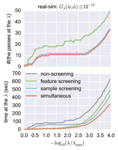
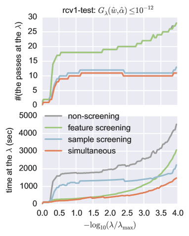
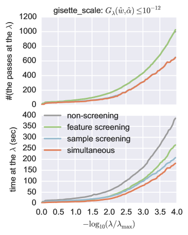
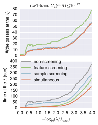
Figure 7: Number of optimization steps and computation time. Sequences of the number of passes through the entire dataset and computation time to convergence for various values of $\lambda$ for classification problems with SPDC solver are plotted.

7 Conclusions

We introduced a new approach for safely screening out features and samples simultaneously. We showed that alternatively iterating feature and sample screening steps has synergetic advantages in that screening performances can be radily improved in steps. We also introduced a new approach for predicting active set without false positive error, which we called safe keeping. Intensive numerical experiments demonstrated the advantage of our approaches in classification and regression problems with large numbers of features and samples.

Appendix A Proofs

A.1 Proof of Lemma 1

Proof.

Since $P_{\lambda}(w)$ is $\lambda$-strongly convex, $\forall w_{1},w_{2}\in{\rm dom}P_{\lambda}$,

$$P_{\lambda}(w_{1})\geq P_{\lambda}(w_{2})+g_{P_{\lambda}}(w_{2})^{\top}(w_{1}-w_{2})+\frac{\lambda}{2}\|w_{1}-w_{2}\|^{2}_{2},$$

where, $g_{P_{\lambda}}(w)\in\partial P_{\lambda}(w)$. On the other hand, $\forall\hat{w}\in{\rm dom}P_{\lambda},$ $g_{P_{\lambda}}(w^{*})^{\top}(\hat{w}-w^{*})\geq 0$ (see Proposition B.24 in [25]). Also, from weak duality, $\forall\hat{\alpha}\in{\rm dom}D_{\lambda},$ $D(\hat{\alpha})\leq P_{\lambda}(w^{*})$. By substituting $w_{1}=\hat{w},w_{2}=w^{*}$,

$$\frac{\lambda}{2}\|\hat{w}-w^{*}\|^{2}_{2}\leq P_{\lambda}(\hat{w})-D_{\lambda}(\hat{\alpha}).$$

Therefore, $w^{*}$ is within a region $\Theta_{w^{*}}$, where

$$\Theta_{w^{*}}:=\set{w}{\|\hat{w}-w\|_{2}\leq\sqrt{2G_{\lambda}(\hat{w},\hat{\alpha})/\lambda}}.$$

Since $\Theta_{w^{*}}$ is Sphere, a lower bound of $x_{i}^{\top}w^{*}$ and an upper bound of $x_{i}^{\top}w^{*}$ are given in closed form as follows:

$$LB(x_{i}^{\top}w^{*}) =x_{i}^{\top}\hat{w}-\|x_{i}\|_{2}\sqrt{2G_{\lambda}(\hat{w},\hat{\alpha})/\lambda},$$

$$UB(x_{i}^{\top}w^{*}) =x_{i}^{\top}\hat{w}+\|x_{i}\|_{2}\sqrt{2G_{\lambda}(\hat{w},\hat{\alpha})/\lambda}.$$

∎

A.2 Proof of Theorem 2

Proof.

Supposing that the result of the previous safe sample screening step assures the optimal values $\alpha_{i}^{*}$ for a subset of the samples $i\in{\cal S}\subset[n]$, the the dual optimal solution region is written as

$$\tilde{\Theta}_{\alpha^{*}}:=\set{\alpha\in\Theta_{\alpha^{*}}}{\alpha_{i}=\alpha^{*}_{i}~{}\forall i\in{\cal S}}.$$

Then, $X_{:j}^{\top}\alpha^{*}$ is bounded from above by the following upper bound:

$$\tilde{UB}(X_{:j}^{\top}\alpha^{*}) :=\max_{\alpha\in\tilde{\Theta}_{\alpha^{*}}}X_{:j}^{\top}\alpha$$

$$=\sum_{i\in{\cal S}}\alpha^{*}_{i}X_{ij}+\max_{\alpha_{{\cal U}_{s}}}X_{:j{\cal U}_{s}}^{\top}\alpha_{{\cal U}_{s}}{\rm~{}~{}s.t~{}}\|\hat{\alpha}_{{\cal U}_{s}}-\alpha_{{\cal U}_{s}}\|^{2}_{2}\leq r_{D}^{2}-\|\hat{\alpha}_{{\cal S}}-\alpha^{*}_{{\cal S}}\|^{2}_{2}$$

$$=\!\sum_{i\in{\cal S}}\!\!\alpha^{*}_{i}X_{ij}\!+\!X_{:j{\cal U}_{s}}^{\top}\hat{\alpha}_{{\cal U}_{s}}\!+\!\|X_{:j{\cal U}_{s}}\|_{2}\sqrt{r_{D}^{2}-\|\hat{\alpha}_{{\cal S}}-\alpha^{*}_{{\cal S}}\|^{2}_{2}}$$

$$=X_{:j}^{\top}\tilde{\alpha}+\|X_{:j{\cal U}_{s}}\|_{2}\sqrt{r_{D}^{2}-\|\hat{\alpha}_{{\cal S}}-\alpha^{*}_{{\cal S}}\|^{2}_{2}}.$$

Similarly, $X_{:j}^{\top}\alpha^{*}$ is bounded from below by the following lower bound:

$$\!\!\tilde{LB}(X_{:j}^{\top}\!\alpha)\!\!:=X_{:j}^{\top}\tilde{\alpha}-\|X_{:j{\cal U}_{s}}\|_{2}\sqrt{r_{D}^{2}-\|\hat{\alpha}_{{\cal S}}-\alpha^{*}_{{\cal S}}\|^{2}_{2}}.$$

Therefore,

$$\tilde{UB}(|X_{:j}^{\top}\alpha|)=|X_{:j}^{\top}\tilde{\alpha}|+\|X_{:j{\cal U}_{s}}\|_{2}\sqrt{r_{D}^{2}-\|\hat{\alpha}_{{\cal S}}-\alpha^{*}_{{\cal S}}\|^{2}_{2}}.$$

Since $\tilde{\Theta}_{\alpha^{*}}\subset{\Theta}_{\alpha^{*}}$, the upper bound in (18) is tighter than or equal to that in (11), i.e., $\tilde{UB}(|X_{:j}^{\top}\alpha^{*}|)\leq UB(|X_{:j}^{\top}\alpha^{*}|)$. ∎

A.3 Proof of Theorem 3

Proof.

Supposing that the result of the previous safe feature screening step assures that $w_{j}^{*}=0$ for a subset of the features $j\in{\cal F}\subset[d]$, the the primal optimal solution region is written as

$$\tilde{\Theta}_{w^{*}}:=\set{w\in\Theta_{w^{*}}}{w_{j}=0~{}\forall j\in{\cal F}}.$$

Then, $x_{i}^{\top}w^{*}$ is bounded from below by the following lower bound:

$$\tilde{LB}(x_{i}^{\top}w) :=\min_{w\in\tilde{\Theta}_{w^{*}}}x_{i}^{\top}w$$

$$=\min_{w}x_{i}^{\top}w{\rm~{}~{}s.t.~{}~{}}\|\hat{w}-w\|_{2}^{2}\leq r_{P}^{2},\hat{w}_{j}=0~{}\forall j\in{\cal F}$$

$$=\min_{w}x_{i{\cal U}_{f}}^{\top}w_{{\cal U}_{f}}{\rm~{}~{}s.t.~{}~{}}\|\hat{w}_{{\cal U}_{f}}-w_{{\cal U}_{f}}\|_{2}^{2}\leq r_{P}^{2}-\|\hat{w}_{\cal F}\|_{2}^{2}$$

$$=x_{i{\cal U}_{f}}^{\top}\hat{w}_{{\cal U}_{f}}-\|x_{i{\cal U}_{f}}\|_{2}\sqrt{r_{P}^{2}-\|\hat{w}_{\cal F}\|_{2}^{2}}.$$

Similarly, $x_{i}^{\top}w^{*}$ is bounded from above by the following upper bound:

$$UB(x_{i}^{\top}w^{*})=x_{i{\cal U}_{f}}^{\top}\hat{w}_{{\cal U}_{f}}+\|x_{i{\cal U}_{f}}\|_{2}\sqrt{r_{P}^{2}-\|\hat{w}_{\cal F}\|_{2}^{2}}.$$

Since $\tilde{\Theta}_{w^{*}}\subset{\Theta}_{w^{*}}$, these bounds in (19) are tighter than or equal to those in (17), i.e., $\tilde{LB}(x_{i}^{\top}w^{*})\geq LB(x_{i}^{\top}w^{*})$ and $\tilde{UB}(x_{i}^{\top}w^{*})\leq UB(x_{i}^{\top}w^{*})$. ∎

A.4 Proof of Theorem 6

We first construct the the dual optimal solution region $\tilde{\Theta}_{\alpha^{*}}$.

Lemma 8.

For an arbitrary pair of primal feasible solution $\hat{w}\in{\rm dom}P_{\lambda}$ and dual feasible solution $\hat{\alpha}\in{\rm dom}D_{\lambda}$, the dual optimal solution region is written as

$$\Theta_{\alpha^{*}}:=\Set{\forall i~{}y_{i}\alpha_{i}\in[0,1]}{y^{\top}\hat{\alpha}\leq y^{\top}\alpha\leq P_{\lambda}(\hat{w})}.$$

Proof of Lemma 8 .

From the optimality and weak duality $y^{\top}\hat{\alpha}\leq y^{\top}\alpha^{*}$ and $y^{\top}\alpha^{*}\leq P_{\lambda}(\hat{w})$, respectively. Therefore,

$$\alpha^{*}\in\hat{\Theta}_{\alpha^{*}}:=\Set{\alpha\in{\rm dom}D_{\lambda}}{y^{\top}\hat{\alpha}\leq y^{\top}\alpha\leq P_{\lambda}(\hat{w})}.$$

Noting that $\hat{\Theta}_{\alpha^{*}}\subseteq\Theta_{\alpha^{*}}$, $\alpha^{*}\in\Theta_{\alpha^{*}}$. ∎

Proof of Theorem 6.

From Lemma 8,

$$X_{:j}^{\top}\alpha^{*}\geq LB(X_{:j}^{\top}\alpha^{*}):=\min_{\alpha\in\Theta_{\alpha^{*}}}X_{:j}^{\top}\alpha$$

Moreover,

$$LB(X_{:j}^{\top}\alpha^{*})=\min_{\alpha\in\Theta_{\alpha^{*}}}Z_{:j}^{\top}\alpha_{y},$$

where $\alpha_{y}$ $:=[y_{1}\alpha_{1},\ldots,y_{n}\alpha_{n}]^{\top}$. Let us define three $n$-dimensional vectors $\bar{\alpha}^{(1)}$, $\bar{\alpha}^{(2)}$ and $\bar{\alpha}^{(3)}$ as follows:

$$\bar{\alpha}^{(1)}_{i} :=\left\{\begin{array}[]{ll}y_{i}&(Z^{\prime}_{ij}<0)\\ 0&(\text{otherwise}),\end{array}\right.$$

$$\bar{\alpha}^{(2)}_{i} :=\left\{\begin{array}[]{ll}y_{i}&(Z^{\prime}_{ij}\leq Z^{\prime}_{l_{q}j})\\ y_{i}(y^{\top}\hat{\alpha}-l_{q})&(Z^{\prime}_{ij}=Z^{\prime}_{(l_{q}+1)j})\\ 0&(otherwise),\end{array}\right.$$

$$\bar{\alpha}^{(3)}_{i} :=\left\{\begin{array}[]{ll}y_{i}&(Z^{\prime}_{ij}\leq Z^{\prime}_{u_{q}j})\\ y_{i}(P_{\lambda}(\hat{w})-u_{q})&(Z^{\prime}_{ij}=Z^{\prime}_{(u_{q}+1)j})\\ 0&(otherwise).\end{array}\right.$$

If $l_{q}+1\leq n_{Z^{\prime}_{:j}}\leq u_{q}$, then $\bar{\alpha}^{(1)}$ is an element of $\Theta_{\alpha^{*}}$ and minimizes $X_{:j}^{\top}\alpha$. If $n_{Z^{\prime}_{:j}}<l_{q}+1$ then $\bar{\alpha}^{(1)}\not\in\Theta_{\alpha^{*}}$, $\bar{\alpha}^{(2)}$ is an element of $\Theta_{\alpha^{*}}$ and minimizes $X_{:j}^{\top}\alpha$ because $y^{\top}\bar{\alpha}^{(2)}=y^{\top}\hat{\alpha}$. If $m_{Z^{\prime}_{:j}}>u_{q}$ then $\bar{\alpha}^{(1)}\not\in\Theta_{\alpha^{*}}$, meaning that $\bar{\alpha}^{(3)}$ is an element of $\Theta_{\alpha^{*}}$ and minimizes $X_{:j}^{\top}\alpha$ because $y^{\top}\bar{\alpha}^{(3)}=P_{\lambda}$. Therefore,

$$LB(X_{:j}^{\top}\alpha^{*}):=\begin{cases}\sum_{i=1}^{l_{q}}Z^{\prime}_{ij}+(y^{\top}\hat{\alpha}-l_{q})Z^{\prime}_{(l_{q}+1)j}&(n_{Z^{\prime}_{:j}}<l_{q}+1),\\ \sum_{i=1}^{u_{q}}Z^{\prime}_{ij}+(P_{\lambda}(\hat{w})-u_{q}),Z^{\prime}_{u_{q}j}&(n_{Z^{\prime}_{:j}}>u_{q})\\ \sum_{i=1}^{n}\min\{0,Z^{\prime}_{ij}\}&({\rm otherwise}),\end{cases}$$

Similarly, from Lemma 8,

$$X_{:j}^{\top}\alpha^{*}\leq UB(X_{:j}^{\top}\alpha^{*}):=\max_{\alpha\in\Theta_{\alpha^{*}}}X_{:j}^{\top}\alpha$$

Moreover,

$$UB(X_{:j}^{\top}\alpha^{*})=\max_{\alpha\in\Theta_{\alpha^{*}}}Z_{:j}^{\top}\alpha_{y}.$$

Let us define three $n$-dimensional vectors $\bar{\alpha}^{(4)}$, $\bar{\alpha}^{(5)}$ and $\bar{\alpha}^{(6)}$ as follows:

$$\bar{\alpha}^{(4)}_{i} :=\left\{\begin{array}[]{ll}y_{i}&(Z^{\prime}_{ij}>0)\\ 0&(\text{otherwise}),\end{array}\right.$$

$$\bar{\alpha}^{(5)}_{i} :=\left\{\begin{array}[]{ll}y_{i}&(Z^{\prime}_{ij}\geq Z^{\prime}_{(n-l_{q})j})\\ y_{i}(y^{\top}\hat{\alpha}-l_{q})&(Z^{\prime}_{ij}=Z^{\prime}_{(n-l_{q}-1)j})\\ 0&(otherwise),\end{array}\right.$$

$$\bar{\alpha}^{(6)}_{i} :=\left\{\begin{array}[]{ll}y_{i}&(Z^{\prime}_{ij}\geq Z^{\prime}_{(n-u_{q})j})\\ y_{i}(P_{\lambda}(\hat{w})-u_{q})&(Z^{\prime}_{ij}=Z^{\prime}_{(n-u_{q}-1)j})\\ 0&(otherwise).\end{array}\right.$$

If $l_{q}+1\leq p_{Z^{\prime}_{:j}}\leq u_{q}$, then $\bar{\alpha}^{(4)}$ is an element of $\Theta_{\alpha^{*}}$ and maximizes $X_{:j}^{\top}\alpha$. If $p_{Z^{\prime}_{:j}}<l_{q}+1$ then $\bar{\alpha}^{(4)}\not\in\Theta_{\alpha^{*}}$, $\bar{\alpha}^{(5)}$ is an element of $\Theta_{\alpha^{*}}$ and maximizes $X_{:j}^{\top}\alpha$ because $y^{\top}\bar{\alpha}^{(5)}=y^{\top}\hat{\alpha}$. If $p_{Z^{\prime}_{:j}}>u_{q}$ then $\bar{\alpha}^{(4)}\not\in\Theta_{\alpha^{*}}$, meaning that $\bar{\alpha}^{(6)}$ is an element of $\Theta_{\alpha^{*}}$ and maximizes $X_{:j}^{\top}\alpha$ because $y^{\top}\bar{\alpha}^{(6)}=P_{\lambda}$. Therefore,

$$UB(X_{:j}^{\top}\alpha^{*}):=\begin{cases}\sum_{i=n-l_{q}}^{n}Z^{\prime}_{ij}+(y^{\top}\hat{\alpha}-l_{q})Z^{\prime}_{(n-l_{q}-1)j}&\!\!\!\!\!\!\!\!(p_{Z^{\prime}_{:j}}<l_{q}+1),\\ \sum_{i=n-u_{q}}^{n}Z^{\prime}_{ij}+(P_{\lambda}(\hat{w})-u_{q})Z^{\prime}_{(n-u_{q}-1)j}&\!\!\!\!(p_{Z^{\prime}_{:j}}>u_{q}),\\ \sum_{i=1}^{n}\max\{0,Z^{\prime}_{ij}\}&\!\!\!\!({\rm otherwise}).\end{cases}$$

On the other hand, from KKT condition(8),

$$\frac{1}{\lambda n}X_{:j}^{\top}\alpha^{*}\in\begin{cases}\frac{w^{*}_{j}}{|w^{*}_{j}|}&(w^{*}_{j}\neq 0)\\ [-1,1]&({\rm otherwise}).\end{cases}$$ (23)

Therefore, if $LB(X_{:j}^{\top}\alpha^{*})<-\lambda n$ and $UB(X_{:j}^{\top}\alpha^{*})>\lambda n$ then $w^{*}_{j}=0$. ∎

A.5 Proof of Theorem 7

First, we construct the primal optimal solution region ${\Theta_{w^{*}}}$.

Lemma 9.

The primal optimal solution region $\Theta_{w^{*}}$ is given $\forall\hat{w}\in{\rm dom}P_{\lambda}$ as

$$\Theta_{w^{*}}=\Set{{w}\in{\rm dom}P_{\lambda}}{\lambda\|w\|_{1}+g_{\ell}(\hat{w})^{\top}w\leq k},$$ (24)

where $g_{\ell}(w):=\frac{1}{n}\sum_{i\in[n]}g_{\ell_{i}}({w})$.

Proof.

From Proposition B.24 in [25],

$$(\lambda g_{\psi}(w^{*})+g_{\ell}(w^{*}))^{\top}(w^{*}-\hat{w})\leq 0,\forall\hat{w}\in{\rm dom}P_{\lambda},$$

where $g_{\psi}(w)\in\partial\psi(w)$. Form the convexity of $\ell_{i}$ for $i\in[n]$ and the definition of subgradient

$$\ell_{i}(w^{*})\geq\ell_{i}(\hat{w})+g_{\ell_{i}}(\hat{w})(w^{*}-\hat{w}),\forall\hat{w}\in{\rm dom}P_{\lambda}$$

$$\ell_{i}(\hat{w})\geq\ell_{i}(w^{*})+g_{\ell_{i}}(w^{*})(\hat{w}-w^{*}),\forall\hat{w}\in{\rm dom}P_{\lambda},$$

and thus, $g_{\ell_{i}}(w^{*})^{\top}(w^{*}-\hat{w})\geq g_{\ell_{i}}(\hat{w})^{\top}(w^{*}-\hat{w}),\forall\hat{w}\in{\rm dom}P_{\lambda}$. Therefore, $\forall\hat{w}\in{\rm dom}P_{\lambda}$,

$$\lambda g_{\psi}(w^{*})^{\top}w^{*}+g_{\ell}(\hat{w})^{\top}w^{*}\leq\lambda g_{\psi}(w^{*})^{\top}\hat{w}+g_{\ell}(\hat{w})^{\top}{\hat{w}}.$$

Since $g_{\psi}(\hat{w})^{\top}\hat{w}=\|\hat{w}\|_{1}=\max_{s\in[-1,1]^{d}}s^{\top}\hat{w}$ and $g_{\psi}(w^{*})\in[-1,1]^{d},$ we have

$$\lambda g_{\psi}(w^{*})^{\top}\hat{w}\leq\lambda g_{\psi}(\hat{w})^{\top}\hat{w}.$$

By combining these results,

$$\lambda\|w^{*}\|_{1}+g_{\ell}(\hat{w})^{\top}w^{*}\leq k,~{}~{}\forall\hat{w}\in{\rm dom}P_{\lambda}.$$

∎

Proof of Theorem 7.

From Lemma 9,

$$x_{i}^{\top}w^{*}\geq LB(x_{i}^{\top}w^{*}):=\min_{w\in\Theta_{w^{*}}}x_{i}^{\top}w.$$

Using a Lagrange multiplier $\mu>0$,

$$LB(x_{i}^{\top}w^{*}) =\min x_{i}^{\top}w~{}~{}{\rm s.t}~{}~{}w\in\Theta_{w^{*}}$$ (25)

$$=\min_{w}\max_{\mu>0}\{x_{i}^{\top}w+\mu(\lambda\|w\|_{1}+g_{\ell}(\hat{w})^{\top}w-k)\}$$

$$=\max_{\mu>0}\{\mu k+\min(\underbrace{x_{i}^{\top}w+\mu\lambda\|w\|_{1}+\frac{\mu}{n}g_{\ell}(\hat{w})^{\top}w}_{L(w)})\}$$

Since $0\in\partial L$, which is written as $\partial L=x_{i}+\mu\lambda\partial\psi(w)+\frac{\mu}{n}g_{\ell}(\hat{w})$, we have

$$\mu\lambda g_{\psi}(w)=-x_{i}-\frac{\mu}{n}g_{\ell}(\hat{w})$$ (26)

Substituting $\mu\lambda\|w\|=-x_{i}^{\top}w-\frac{\mu}{n}g_{\ell}(\hat{w})^{\top}w$ into (25),

$$LB(x_{i}^{\top}w^{*})=\max_{\mu>0}\{\mu k\}~{}~{}{\rm s.t.}~{}~{}\|-\frac{1}{\lambda}x_{i}^{\top}w-\frac{\mu}{\lambda n}g_{\ell}(\hat{w})^{\top}w\|_{\infty}\leq\mu,$$

where the constraint comes from (26). Similarly, since

$$x_{i}^{\top}w^{*}\leq UB(x_{i}^{\top}w^{*}):=\max_{w\in\Theta_{w^{*}}}x_{i}^{\top}w=-\min_{w\in\Theta_{w^{*}}}x_{i}^{\top}w,$$

$$UB(x_{i}^{\top}w^{*})=\max_{\mu>0}\{\mu k\}~{}~{}{\rm s.t.}~{}~{}\|\frac{1}{\lambda}x_{i}^{\top}w-\frac{\mu}{\lambda n}g_{\ell}(\hat{w})^{\top}w\|_{\infty}\leq\mu.$$

∎

Appendix B Safe keeping by using KKT optimality conditions

In this appendix, we describe another type of safe keeping approaches based on KKT optimality conditions.

Theorem 10.

For an arbitrary pair of primal feasible solution $\hat{w}\in{\rm dom}P_{\lambda}$ and dual feasible solution $\hat{\alpha}\in{\rm dom}D_{\lambda}$,

$$LB(X_{:j}^{\top}\alpha^{*})<-\lambda n~{}{\rm and}~{}\lambda n<UB(X_{:j}^{\top}\alpha^{*})~{}\Rightarrow~{}w_{j}^{*}\neq 0$$

for $j\in[d]$, where

$$LB(X_{:j}^{\top}\alpha^{*}) :=X_{:j}^{\top}\hat{\alpha}-\|X_{:j}\|_{2}\sqrt{2nG_{\lambda}(\hat{w},\hat{\alpha})/\gamma},$$

$$UB(X_{:j}^{\top}\alpha^{*}) :=X_{:j}^{\top}\hat{\alpha}+\|X_{:j}\|_{2}\sqrt{2nG_{\lambda}(\hat{w},\hat{\alpha})/\gamma}.$$

Proof.

In the case that $D_{\lambda}$ is $\gamma/n$-strongly concave, $X_{:j}^{\top}\alpha^{*}$ is bounded from below and above respectively by the following lower and upper bounds:

$$LB(X_{:j}^{\top}\alpha^{*}) :=X_{:j}^{\top}\hat{\alpha}-\|X_{:j}\|_{2}\sqrt{2nG_{\lambda}(\hat{w},\hat{\alpha})/\gamma},$$

$$UB(X_{:j}^{\top}\alpha^{*}) :=X_{:j}^{\top}\hat{\alpha}+\|X_{:j}\|_{2}\sqrt{2nG_{\lambda}(\hat{w},\hat{\alpha})/\gamma}.$$

On the other hand, in the case of our specific regularization term (2), from KKT optimality condition (8), if $-\lambda n<X_{:j}^{\top}\alpha^{*}<\lambda n$ then $w^{*}_{j}\neq 0$.

Therefore,

$$LB(X_{:j}^{\top}\alpha^{*})<-\lambda n~{}{\rm and}~{}\lambda n<UB(X_{:j}^{\top}\alpha^{*})~{}\Rightarrow~{}w_{j}^{*}\neq 0$$

∎

Similarly, we can develop safe sample keeping based on KKT optimiality condition.

Theorem 11.

For an arbitrary pair of primal feasible solution $\hat{w}\in{\rm dom}P_{\lambda}$ and dual feasible solution $\hat{\alpha}\in{\rm dom}D_{\lambda}$, if $\ell_{i}$ is smoothed hinge loss then, for $y_{i}=+1$,

$$1-\gamma<LB(x_{i}^{\top}w^{*})~{}{\rm and}~{}UB(x_{i}^{\top}w^{*})<1~{}\Rightarrow~{}\alpha^{*}_{i}\not\in\{0,+1\},$$

and, for $y_{i}=-1$,

$$-1<LB(x_{i}^{\top}w^{*})~{}{\rm and}~{}UB(x_{i}^{\top}w^{*})<\gamma-1~{}\Rightarrow~{}\alpha^{*}_{i}\not\in\{-1,0\}.$$

If $\ell_{i}$ is smoothed $\varepsilon$-insensitive loss then

$$-\gamma+y_{i}-\varepsilon<LB(x_{i}^{\top}w^{*})~{} {\rm and}~{}UB(x_{i}^{\top}w^{*})<y_{i}-\varepsilon$$

$$~{}{\rm or}~{}$$

$$y_{i}+\varepsilon<LB(x_{i}^{\top}w^{*})~{} {\rm and}~{}UB(x_{i}^{\top}w^{*})<\gamma+y_{i}+\varepsilon$$

$$~{}\Rightarrow~{}\alpha^{*}_{i} \not\in\{-1,0,+1\},$$

for $j\in[d]$, where

$$LB(x_{i}^{\top}w^{*}) =x_{i}^{\top}\hat{w}-\|x_{i}\|_{2}\sqrt{2G_{\lambda}(\hat{w},\hat{\alpha})/\lambda},$$

$$UB(x_{i}^{\top}w^{*}) =x_{i}^{\top}\hat{w}+\|x_{i}\|_{2}\sqrt{2G_{\lambda}(\hat{w},\hat{\alpha})/\lambda}.$$

Proof.

In the case that $P_{\lambda}$ is $\lambda$-strongly convex, $x_{i}^{\top}w^{*}$ is bounded from below and above respectively by the following lower and upper bounds:

$$LB(x_{i}^{\top}w^{*}) =x_{i}^{\top}\hat{w}-\|x_{i}\|_{2}\sqrt{2G_{\lambda}(\hat{w},\hat{\alpha})/\lambda},$$

$$UB(x_{i}^{\top}w^{*}) =x_{i}^{\top}\hat{w}+\|x_{i}\|_{2}\sqrt{2G_{\lambda}(\hat{w},\hat{\alpha})/\lambda}.$$

On the other hand, from KKT optimality condition (8), in the case of smoothed hinge loss (3), if $y_{i}=+1$ and $1-\gamma<x_{i}^{\top}w^{*}<1$ then $\alpha^{*}_{i}\in\{0,+1\}$, if $y_{i}=1$ and $-1<x_{i}^{\top}w^{*}<\gamma-1$ then $\alpha^{*}_{i}\in\{-1,0\}$. Therefore,

$$y_{i}=+1~{}{\rm and}~{}1-\gamma<LB(x_{i}^{\top}w^{*})~{}{\rm and}~{}UB(x_{i}^{\top}w^{*})<1$$

$$~{}\Rightarrow~{}\alpha^{*}_{i}\not\in\{0,+1\},$$

$$y_{i}=-1~{}{\rm and}~{}-1<LB(x_{i}^{\top}w^{*})~{}{\rm and}~{}UB(x_{i}^{\top}w^{*})<\gamma-1$$

$$~{}\Rightarrow~{}\alpha^{*}_{i}\not\in\{-1,0\}.$$

Also, in the case of smoothed $\varepsilon$-insensitive (4), if $-\gamma+y_{i}-\varepsilon<x_{i}^{\top}w^{*}<y_{i}-\varepsilon$ or $y_{i}+\varepsilon<x_{i}^{\top}w^{*}<\gamma+y_{i}+\varepsilon$ then, $\alpha^{*}_{i}\not\in\{-1,0,+1\}$ . Therefore,

$$-\gamma+y_{i}-\varepsilon<LB(x_{i}^{\top}w^{*})~{} {\rm and}~{}UB(x_{i}^{\top}w^{*})<y_{i}-\varepsilon$$

$$~{}{\rm or}~{}$$

$$y_{i}+\varepsilon<LB(x_{i}^{\top}w^{*})~{} {\rm and}~{}UB(x_{i}^{\top}w^{*})<\gamma+y_{i}+\varepsilon~{}\Rightarrow~{}\alpha^{*}_{i}\not\in\{-1,0,+1\},$$

∎

References

• [1] Trevor Hastie, Robert Tibshirani, and Martin Wainwright. Statistical Learning with Sparsity: The Lasso and Generalizations. CRC Press, 2015.
• [2] Robert Tibshirani. Regression shrinkage and selection via the lasso. Journal of the Royal Statistical Society. Series B (Methodological), pages 267–288, 1996.
• [3] Bernhard E Boser, Isabelle M Guyon, and Vladimir N Vapnik. A training algorithm for optimal margin classifiers. In Proceedings of the fifth annual workshop on Computational learning theory, pages 144–152. ACM, 1992.
• [4] Chih-Chung Chang and Chih-Jen Lin. Libsvm: A library for support vector machines. ACM Transactions on Intelligent Systems and Technology (TIST), 2(3):27, 2011.
• [5] Laurent El Ghaoui, Vivian Viallon, and Tarek Rabbani. Safe feature elimination for the lasso and sparse supervised learning problems. Pacific Journal of Optimization, 8(4):667–698, 2012.
• [6] Zhen J Xiang, Hao Xu, and Peter J Ramadge. Learning sparse representations of high dimensional data on large scale dictionaries. In Advances in Neural Information Processing Systems, pages 900–908, 2011.
• [7] Jie Wang, Jiayu Zhou, Peter Wonka, and Jieping Ye. Lasso screening rules via dual polytope projection. In Advances in Neural Information Processing Systems, pages 1070–1078, 2013.
• [8] Antoine Bonnefoy, Valentin Emiya, Liva Ralaivola, and Rémi Gribonval. A dynamic screening principle for the lasso. In Signal Processing Conference (EUSIPCO), 2014 Proceedings of the 22nd European, pages 6–10. IEEE, 2014.
• [9] Jun Liu, Zheng Zhao, Jie Wang, and Jieping Ye. Safe Screening with Variational Inequalities and Its Application to Lasso. In Proceedings of the 31st International Conference on Machine Learning, 2014.
• [10] Jie Wang, Jiayu Zhou, Jun Liu, Peter Wonka, and Jieping Ye. A safe screening rule for sparse logistic regression. In Advances in Neural Information Processing Systems, pages 1053–1061, 2014.
• [11] Zhen James Xiang, Yun Wang, and Peter J Ramadge. Screening tests for lasso problems. arXiv preprint arXiv:1405.4897, 2014.
• [12] Olivier Fercoq, Alexandre Gramfort, and Joseph Salmon. Mind the duality gap: safer rules for the lasso. In Proceedings of the 32nd International Conference on Machine Learning, pages 333–342, 2015.
• [13] Eugene Ndiaye, Olivier Fercoq, Alexandre Gramfort, and Joseph Salmon. Gap safe screening rules for sparse multi-task and multi-class models. In Advances in Neural Information Processing Systems, pages 811–819, 2015.
• [14] Kohei Ogawa, Yoshiki Suzuki, and Ichiro Takeuchi. Safe screening of non-support vectors in pathwise svm computation. In Proceedings of the 30th International Conference on Machine Learning, pages 1382–1390, 2013.
• [15] Jie Wang, Peter Wonka, and Jieping Ye. Scaling svm and least absolute deviations via exact data reduction. Proceedings of The 31st International Conference on Machine Learning, 2014.
• [16] Julian Zimmert, Christian Schroeder de Witt, Giancarlo Kerg, and Marius Kloft. Safe screening for support vector machines. NIPS 2015 Workshop on Optimization in Machine Learning (OPT), 2015.
• [17] Shai Shalev-Shwartz and Tong Zhang. Accelerated proximal stochastic dual coordinate ascent for regularized loss minimization. Mathematical Programming, pages 1–41, 2015.
• [18] Ralph Tyrell Rockafellar. Convex analysis. Princeton university press, 1970.
• [19] Paul S Bradley and Olvi L Mangasarian. Feature selection via concave minimization and support vector machines. In ICML, volume 98, pages 82–90, 1998.
• [20] Ji Zhu, Saharon Rosset, Trevor Hastie, and Rob Tibshirani. 1-norm support vector machines. Advances in neural information processing systems, 16(1):49–56, 2004.
• [21] Ayhan Demiriz, Kristin P Bennett, and John Shawe-Taylor. Linear programming boosting via column generation. Machine Learning, 46(1-3):225–254, 2002.
• [22] Manfred Warmuth, Karen Glocer, and S V N Vishwanathan. Entropy Regularized LPBoost. In Proceedings of the 19th International Conference on Algorithmic Learning Theory, volume 5254 of LNCS, pages 256–271, 2008.
• [23] Kohei Hatano and Eiji Takimoto. Linear Programming Boosting by Column and Row Generation. In Proceedings of the 12th International Conference on Dicovery Science (DS 2009), volume 5808 of LNCS, pages 401–408, 2009.
• [24] Yuchen Zhang and Xiao Lin. Stochastic primal-dual coordinate method for regularized empirical risk minimization. Proceedings of The 32nd International Conference on Machine Learning, pages 353–361, 2015.
• [25] D. P. Bertsekas. Nonlinear Programming (2nd edition). Athena Scientific, 1999.