Two-sample tests for high-dimension,
strongly spiked eigenvalue models
Makoto Aoshima and Kazuyoshi Yata
University of Tsukuba
Abstract:
We consider two-sample tests for high-dimensional data under two disjoint models: the strongly spiked eigenvalue (SSE) model and the non-SSE (NSSE) model.
We provide a general test statistic as a function of a positive-semidefinite matrix.
We give sufficient conditions for the test statistic to satisfy a consistency property and to be asymptotically normal.
We discuss an optimality of the test statistic under the NSSE model.
We also investigate the test statistic under the SSE model by considering strongly spiked eigenstructures and create a new effective test procedure for the SSE model.
Finally, we discuss the performance of the classifiers numerically.
Key words and phrases:
Asymptotic normality, eigenstructure estimation, large p 𝑝 p n 𝑛 n
A common feature of high-dimensional data is that the data dimension is high, however, the sample size is relatively low.
This is the so-called “HDLSS” or “large p 𝑝 p n 𝑛 n p 𝑝 p n 𝑛 n p / n → ∞ → 𝑝 𝑛 p/n\to\infty p 𝑝 p π i , i = 1 , 2 formulae-sequence subscript 𝜋 𝑖 𝑖
1 2 \pi_{i},\ i=1,2 𝝁 i subscript 𝝁 𝑖 \mbox{\boldmath$\mu$}_{i} 𝚺 i subscript 𝚺 𝑖 \mbox{\boldmath$\Sigma$}_{i} π i subscript 𝜋 𝑖 \pi_{i} 𝚺 i subscript 𝚺 𝑖 \mbox{\boldmath$\Sigma$}_{i} ( i = 1 , 2 ) 𝑖 1 2
(i=1,2) 𝚺 i = 𝑯 i 𝚲 i 𝑯 i T = ∑ j = 1 p λ i j 𝒉 i j 𝒉 i j T subscript 𝚺 𝑖 subscript 𝑯 𝑖 subscript 𝚲 𝑖 superscript subscript 𝑯 𝑖 𝑇 superscript subscript 𝑗 1 𝑝 subscript 𝜆 𝑖 𝑗 subscript 𝒉 𝑖 𝑗 superscript subscript 𝒉 𝑖 𝑗 𝑇 \mbox{\boldmath$\Sigma$}_{i}=\mbox{\boldmath{$H$}}_{i}\mbox{\boldmath$\Lambda$}_{i}\mbox{\boldmath{$H$}}_{i}^{T}=\sum_{j=1}^{p}\lambda_{ij}\mbox{\boldmath{$h$}}_{ij}\mbox{\boldmath{$h$}}_{ij}^{T} 𝚲 i = diag ( λ i 1 , … , λ i p ) subscript 𝚲 𝑖 diag subscript 𝜆 𝑖 1 … subscript 𝜆 𝑖 𝑝 \mbox{\boldmath$\Lambda$}_{i}=\mbox{diag}(\lambda_{i1},...,\lambda_{ip}) λ i 1 ≥ ⋯ ≥ λ i p > 0 subscript 𝜆 𝑖 1 ⋯ subscript 𝜆 𝑖 𝑝 0 \lambda_{i1}\geq\cdots\geq\lambda_{ip}>0 𝑯 i = [ 𝒉 i 1 , … , 𝒉 i p ] subscript 𝑯 𝑖 subscript 𝒉 𝑖 1 … subscript 𝒉 𝑖 𝑝
\mbox{\boldmath{$H$}}_{i}=[\mbox{\boldmath{$h$}}_{i1},...,\mbox{\boldmath{$h$}}_{ip}] λ i 1 subscript 𝜆 𝑖 1 \lambda_{i1} 𝚺 i subscript 𝚺 𝑖 \mbox{\boldmath$\Sigma$}_{i} i = 1 , 2 𝑖 1 2
i=1,2 1.6 1.4
In this paper, we consider the two-sample test:
H 0 : 𝝁 1 = 𝝁 2 vs. H 1 : 𝝁 1 ≠ 𝝁 2 . : subscript 𝐻 0 subscript 𝝁 1 subscript 𝝁 2 vs. subscript 𝐻 1
: subscript 𝝁 1 subscript 𝝁 2 H_{0}:\mbox{\boldmath$\mu$}_{1}=\mbox{\boldmath$\mu$}_{2}\quad\mbox{vs.}\quad H_{1}:\mbox{\boldmath$\mu$}_{1}\neq\mbox{\boldmath$\mu$}_{2}. (1.1)
Having recorded i.i.d. samples, 𝒙 i j , j = 1 , … , n i formulae-sequence subscript 𝒙 𝑖 𝑗 𝑗
1 … subscript 𝑛 𝑖
\mbox{\boldmath{$x$}}_{ij},\ j=1,...,n_{i} n i subscript 𝑛 𝑖 n_{i} π i subscript 𝜋 𝑖 \pi_{i} 𝒙 ¯ i n i = ∑ j = 1 n i 𝒙 i j / n i subscript ¯ 𝒙 𝑖 subscript 𝑛 𝑖 superscript subscript 𝑗 1 subscript 𝑛 𝑖 subscript 𝒙 𝑖 𝑗 subscript 𝑛 𝑖 \overline{\mbox{\boldmath{$x$}}}_{in_{i}}=\sum_{j=1}^{n_{i}}\mbox{\boldmath{$x$}}_{ij}/n_{i} 𝑺 i n i = ∑ j = 1 n i ( 𝒙 i j − 𝒙 ¯ i n i ) ( 𝒙 i j − 𝒙 ¯ i n i ) T / ( n i − 1 ) subscript 𝑺 𝑖 subscript 𝑛 𝑖 superscript subscript 𝑗 1 subscript 𝑛 𝑖 subscript 𝒙 𝑖 𝑗 subscript ¯ 𝒙 𝑖 subscript 𝑛 𝑖 superscript subscript 𝒙 𝑖 𝑗 subscript ¯ 𝒙 𝑖 subscript 𝑛 𝑖 𝑇 subscript 𝑛 𝑖 1 \mbox{\boldmath{$S$}}_{in_{i}}=\sum_{j=1}^{n_{i}}(\mbox{\boldmath{$x$}}_{ij}-\overline{\mbox{\boldmath{$x$}}}_{in_{i}})(\mbox{\boldmath{$x$}}_{ij}-\overline{\mbox{\boldmath{$x$}}}_{in_{i}})^{T}/(n_{i}-1) i = 1 , 2 𝑖 1 2
i=1,2 n i ≥ 4 subscript 𝑛 𝑖 4 n_{i}\geq 4 i = 1 , 2 𝑖 1 2
i=1,2 T 2 superscript 𝑇 2 T^{2}
T 2 = ( n 1 + n 2 ) − 1 n 1 n 2 ( 𝒙 ¯ 1 n 1 − 𝒙 ¯ 2 n 2 ) T 𝑺 − 1 ( 𝒙 ¯ 1 n 1 − 𝒙 ¯ 2 n 2 ) , superscript 𝑇 2 superscript subscript 𝑛 1 subscript 𝑛 2 1 subscript 𝑛 1 subscript 𝑛 2 superscript subscript ¯ 𝒙 1 subscript 𝑛 1 subscript ¯ 𝒙 2 subscript 𝑛 2 𝑇 superscript 𝑺 1 subscript ¯ 𝒙 1 subscript 𝑛 1 subscript ¯ 𝒙 2 subscript 𝑛 2 T^{2}=(n_{1}+n_{2})^{-1}n_{1}n_{2}(\overline{\mbox{\boldmath{$x$}}}_{1n_{1}}-\overline{\mbox{\boldmath{$x$}}}_{2n_{2}})^{T}\mbox{\boldmath{$S$}}^{-1}(\overline{\mbox{\boldmath{$x$}}}_{1n_{1}}-\overline{\mbox{\boldmath{$x$}}}_{2n_{2}}),
where 𝑺 = { ( n 1 − 1 ) 𝑺 1 n 1 + ( n 2 − 1 ) 𝑺 2 n 2 } / ( n 1 + n 2 − 2 ) 𝑺 subscript 𝑛 1 1 subscript 𝑺 1 subscript 𝑛 1 subscript 𝑛 2 1 subscript 𝑺 2 subscript 𝑛 2 subscript 𝑛 1 subscript 𝑛 2 2 \mbox{\boldmath{$S$}}=\{(n_{1}-1)\mbox{\boldmath{$S$}}_{1n_{1}}+(n_{2}-1)\mbox{\boldmath{$S$}}_{2n_{2}}\}/(n_{1}+n_{2}-2) 𝑺 − 1 superscript 𝑺 1 \mbox{\boldmath{$S$}}^{-1} p / n i → ∞ , i = 1 , 2 formulae-sequence → 𝑝 subscript 𝑛 𝑖 𝑖 1 2
p/n_{i}\to\infty,\ i=1,2 Dempster (1958 , 1960 ) and Srivastava (2007 ) considered the test when π 1 subscript 𝜋 1 \pi_{1} π 2 subscript 𝜋 2 \pi_{2} π 1 subscript 𝜋 1 \pi_{1} π 2 subscript 𝜋 2 \pi_{2} Bai and Saranadasa (1996 ) and Cai, Liu, and Xia (2014 ) considered the test under homoscedasticity, 𝚺 1 = 𝚺 2 subscript 𝚺 1 subscript 𝚺 2 \mbox{\boldmath$\Sigma$}_{1}=\mbox{\boldmath$\Sigma$}_{2} Chen and Qin (2010 ) and Aoshima and Yata (2011 , 2015 ) considered the test under heteroscedasticity, 𝚺 1 ≠ 𝚺 2 subscript 𝚺 1 subscript 𝚺 2 \mbox{\boldmath$\Sigma$}_{1}\neq\mbox{\boldmath$\Sigma$}_{2}
In this paper, we first consider the following test statistic with a positive-semidefinite matrix 𝑨 𝑨 A p 𝑝 p
T ( 𝑨 ) 𝑇 𝑨 \displaystyle T(\mbox{\boldmath{$A$}}) = ( 𝒙 ¯ 1 n 1 − 𝒙 ¯ 2 n 2 ) T 𝑨 ( 𝒙 ¯ 1 n 1 − 𝒙 ¯ 2 n 2 ) − ∑ i = 1 2 tr ( 𝑺 i n i 𝑨 ) / n i absent superscript subscript ¯ 𝒙 1 subscript 𝑛 1 subscript ¯ 𝒙 2 subscript 𝑛 2 𝑇 𝑨 subscript ¯ 𝒙 1 subscript 𝑛 1 subscript ¯ 𝒙 2 subscript 𝑛 2 superscript subscript 𝑖 1 2 tr subscript 𝑺 𝑖 subscript 𝑛 𝑖 𝑨 subscript 𝑛 𝑖 \displaystyle=(\overline{\mbox{\boldmath{$x$}}}_{1n_{1}}-\overline{\mbox{\boldmath{$x$}}}_{2n_{2}})^{T}\mbox{\boldmath{$A$}}(\overline{\mbox{\boldmath{$x$}}}_{1n_{1}}-\overline{\mbox{\boldmath{$x$}}}_{2n_{2}})-\sum_{i=1}^{2}\mbox{tr}(\mbox{\boldmath{$S$}}_{in_{i}}\mbox{\boldmath{$A$}})/n_{i}
= 2 ∑ i = 1 2 ∑ j < j ′ n i 𝒙 i j T 𝑨 𝒙 i j ′ n i ( n i − 1 ) − 2 𝒙 ¯ 1 n 1 T 𝑨 𝒙 ¯ 2 n 2 . absent 2 superscript subscript 𝑖 1 2 superscript subscript 𝑗 superscript 𝑗 ′ subscript 𝑛 𝑖 superscript subscript 𝒙 𝑖 𝑗 𝑇 subscript 𝑨 𝒙 𝑖 superscript 𝑗 ′ subscript 𝑛 𝑖 subscript 𝑛 𝑖 1 2 superscript subscript ¯ 𝒙 1 subscript 𝑛 1 𝑇 𝑨 subscript ¯ 𝒙 2 subscript 𝑛 2 \displaystyle=2\sum_{i=1}^{2}\frac{\sum_{j<j^{\prime}}^{n_{i}}\mbox{\boldmath{$x$}}_{ij}^{T}\mbox{\boldmath{$A$}}\mbox{\boldmath{$x$}}_{ij^{\prime}}}{n_{i}(n_{i}-1)}-2\overline{\mbox{\boldmath{$x$}}}_{1n_{1}}^{T}\mbox{\boldmath{$A$}}\overline{\mbox{\boldmath{$x$}}}_{2n_{2}}. (1.2)
Note that E { T ( 𝑨 ) } = ( 𝝁 1 − 𝝁 2 ) T 𝑨 ( 𝝁 1 − 𝝁 2 ) 𝐸 𝑇 𝑨 superscript subscript 𝝁 1 subscript 𝝁 2 𝑇 𝑨 subscript 𝝁 1 subscript 𝝁 2 E\{T(\mbox{\boldmath{$A$}})\}=(\mbox{\boldmath$\mu$}_{1}-\mbox{\boldmath$\mu$}_{2})^{T}\mbox{\boldmath{$A$}}(\mbox{\boldmath$\mu$}_{1}-\mbox{\boldmath$\mu$}_{2}) 𝑰 p subscript 𝑰 𝑝 \mbox{\boldmath{$I$}}_{p} p 𝑝 p T ( 𝑰 p ) 𝑇 subscript 𝑰 𝑝 T(\mbox{\boldmath{$I$}}_{p}) Chen and Qin (2010 ) and Aoshima and Yata (2011 ) .
We call the test with T ( 𝑰 p ) 𝑇 subscript 𝑰 𝑝 T(\mbox{\boldmath{$I$}}_{p}) 𝑨 𝑨 A p → ∞ → 𝑝 p\to\infty n 1 → ∞ → subscript 𝑛 1 n_{1}\to\infty n 2 → ∞ → subscript 𝑛 2 n_{2}\to\infty
m → ∞ , where m = min { p , n min } with n min = min { n 1 , n 2 } . → 𝑚 where m = min { p , n min } with n min = min { n 1 , n 2 }
m\to\infty,\quad\mbox{where \ $m=\min\{p,n_{\min}\}$ \ with \ $n_{\min}=\min\{n_{1},n_{2}\}$}.
By using Theorem 1 in Chen and Qin (2010 ) or Theorem 4 in Aoshima and Yata (2015 ) , we can claim that under H 0 subscript 𝐻 0 H_{0} 1.1
T ( 𝑰 p ) / { K 1 ( 𝑰 p ) } 1 / 2 ⇒ N ( 0 , 1 ) as m → ∞ ⇒ 𝑇 subscript 𝑰 𝑝 superscript subscript 𝐾 1 subscript 𝑰 𝑝 1 2 𝑁 0 1 as m → ∞
T(\mbox{\boldmath{$I$}}_{p})/\{K_{1}(\mbox{\boldmath{$I$}}_{p})\}^{1/2}\Rightarrow N(0,1)\ \ \mbox{as $m\to\infty$} (1.3)
if we assume (A-i) that is given in Section 2 and the condition that
λ i 1 2 tr ( 𝚺 i 2 ) → 0 as p → ∞ for i = 1 , 2 . → superscript subscript 𝜆 𝑖 1 2 tr superscript subscript 𝚺 𝑖 2 0 as p → ∞ for i = 1 , 2 .
\frac{\lambda_{i1}^{2}}{\mbox{tr}(\mbox{\boldmath$\Sigma$}_{i}^{2})}\to 0\ \ \mbox{as $p\to\infty$ for $i=1,2$.} (1.4)
Here, K 1 ( 𝑨 ) subscript 𝐾 1 𝑨 K_{1}(\mbox{\boldmath{$A$}}) ⇒ ⇒ \Rightarrow N ( 0 , 1 ) 𝑁 0 1 N(0,1) T ( 𝑰 p ) 𝑇 subscript 𝑰 𝑝 T(\mbox{\boldmath{$I$}}_{p}) K 1 ( 𝑰 p ) subscript 𝐾 1 subscript 𝑰 𝑝 K_{1}(\mbox{\boldmath{$I$}}_{p}) 1.1 Aoshima and Yata (2015 ) , the distance-based two-sample test is quite flexible for high-dimension, non-Gaussian data.
In Section 3, we shall investigate an optimality of the test statistic in (1.2 𝑨 𝑨 A
For eigenvalues of high-dimensional data, Jung and Marron (2009 ) , Yata and Aoshima (2012 , 2013b ) , Onatski (2012 ) and Fan, Liao, and Mincheva (2013 ) considered spiked models such as λ i j → ∞ → subscript 𝜆 𝑖 𝑗 \lambda_{ij}\to\infty p → ∞ → 𝑝 p\to\infty j = 1 , … , k i 𝑗 1 … subscript 𝑘 𝑖
j=1,...,k_{i} k i subscript 𝑘 𝑖 k_{i}
lim inf p → ∞ { λ i 1 2 tr ( 𝚺 i 2 ) } > 0 for i = 1 or 2. subscript limit-infimum → 𝑝 superscript subscript 𝜆 𝑖 1 2 tr superscript subscript 𝚺 𝑖 2 0 for i = 1 or 2.
\liminf_{p\to\infty}\Big{\{}\frac{\lambda_{i1}^{2}}{\mbox{tr}(\mbox{\boldmath$\Sigma$}_{i}^{2})}\Big{\}}>0\ \ \mbox{for $i=1$ or 2.} (1.6)
In (1.6 1.4 1.6 1.5 α i 1 ≥ 1 / 2 subscript 𝛼 𝑖 1 1 2 \alpha_{i1}\geq 1/2 1.6 1.3 Katayama, Kano and Srivastava (2013 ) and Ma, Lan and Wang (2015 ) .
Recall that (1.3 1.4 1.4
The organization of this paper is as follows.
In Section 2, we give sufficient conditions for T ( 𝑨 ) 𝑇 𝑨 T(\mbox{\boldmath{$A$}}) T ( 𝑨 ) 𝑇 𝑨 T(\mbox{\boldmath{$A$}}) 𝑨 𝑨 A
2. Asymptotic Properties of T ( A ) 𝑇 𝐴 T(\mbox{\boldmath{$A$}})
In this section, we give sufficient conditions for T ( 𝑨 ) 𝑇 𝑨 T(\mbox{\boldmath{$A$}}) 𝑨 𝑨 A 𝑨 𝑨 A 𝑨 1 / 2 superscript 𝑨 1 2 \mbox{\boldmath{$A$}}^{1/2} 𝒙 i j = 𝑯 i 𝚲 i 1 / 2 𝒛 i j + 𝝁 i subscript 𝒙 𝑖 𝑗 subscript 𝑯 𝑖 superscript subscript 𝚲 𝑖 1 2 subscript 𝒛 𝑖 𝑗 subscript 𝝁 𝑖 \mbox{\boldmath{$x$}}_{ij}=\mbox{\boldmath{$H$}}_{i}\mbox{\boldmath$\Lambda$}_{i}^{1/2}\mbox{\boldmath{$z$}}_{ij}+\mbox{\boldmath$\mu$}_{i} 𝒛 i j = ( z i 1 j , … , z i p j ) T subscript 𝒛 𝑖 𝑗 superscript subscript 𝑧 𝑖 1 𝑗 … subscript 𝑧 𝑖 𝑝 𝑗 𝑇 \mbox{\boldmath{$z$}}_{ij}=(z_{i1j},...,z_{ipj})^{T} 𝒛 i j subscript 𝒛 𝑖 𝑗 \mbox{\boldmath{$z$}}_{ij}
𝒙 i j = 𝚪 i 𝒘 i j + 𝝁 i for i = 1 , 2 ; j = 1 , … , n i , formulae-sequence subscript 𝒙 𝑖 𝑗 subscript 𝚪 𝑖 subscript 𝒘 𝑖 𝑗 subscript 𝝁 𝑖 for 𝑖 1 2 𝑗
1 … subscript 𝑛 𝑖
\mbox{\boldmath{$x$}}_{ij}=\mbox{\boldmath$\Gamma$}_{i}\mbox{\boldmath{$w$}}_{ij}+\mbox{\boldmath$\mu$}_{i}\ \mbox{ for }i=1,2;\ j=1,...,n_{i}, (2.1)
where 𝚪 i subscript 𝚪 𝑖 \mbox{\boldmath$\Gamma$}_{i} p × r i 𝑝 subscript 𝑟 𝑖 p\times r_{i} r i ≥ p subscript 𝑟 𝑖 𝑝 r_{i}\geq p 𝚪 i 𝚪 i T = 𝚺 i subscript 𝚪 𝑖 superscript subscript 𝚪 𝑖 𝑇 subscript 𝚺 𝑖 \mbox{\boldmath$\Gamma$}_{i}\mbox{\boldmath$\Gamma$}_{i}^{T}=\mbox{\boldmath$\Sigma$}_{i} 𝒘 i j , j = 1 , … , n i formulae-sequence subscript 𝒘 𝑖 𝑗 𝑗
1 … subscript 𝑛 𝑖
\mbox{\boldmath{$w$}}_{ij},\ j=1,...,n_{i} E ( 𝒘 i j ) = 𝟎 𝐸 subscript 𝒘 𝑖 𝑗 0 E(\mbox{\boldmath{$w$}}_{ij})=\mbox{\boldmath{$0$}} ( 𝒘 i j ) = 𝑰 r i subscript 𝒘 𝑖 𝑗 subscript 𝑰 subscript 𝑟 𝑖 (\mbox{\boldmath{$w$}}_{ij})=\mbox{\boldmath{$I$}}_{r_{i}} 2.1 𝚪 i = 𝑯 i 𝚲 i 1 / 2 subscript 𝚪 𝑖 subscript 𝑯 𝑖 superscript subscript 𝚲 𝑖 1 2 \mbox{\boldmath$\Gamma$}_{i}=\mbox{\boldmath{$H$}}_{i}\mbox{\boldmath$\Lambda$}_{i}^{1/2} 𝒘 i j = 𝒛 i j subscript 𝒘 𝑖 𝑗 subscript 𝒛 𝑖 𝑗 \mbox{\boldmath{$w$}}_{ij}=\mbox{\boldmath{$z$}}_{ij} Bai and Saranadasa (1996 ) , Chen and Qin (2010 ) and Aoshima and Yata (2015 ) for the details of the model.
As for 𝒘 i j = ( w i 1 j , … , w i r i j ) T subscript 𝒘 𝑖 𝑗 superscript subscript 𝑤 𝑖 1 𝑗 … subscript 𝑤 𝑖 subscript 𝑟 𝑖 𝑗 𝑇 \mbox{\boldmath{$w$}}_{ij}=(w_{i1j},...,w_{ir_{i}j})^{T} π i , i = 1 , 2 formulae-sequence subscript 𝜋 𝑖 𝑖
1 2 \pi_{i},\ i=1,2
(A-i)
The fourth moments of each variable in 𝒘 i j subscript 𝒘 𝑖 𝑗 \mbox{\boldmath{$w$}}_{ij} E ( w i s j 2 w i t j 2 ) = E ( w i s j 2 ) E ( w i t j 2 ) 𝐸 superscript subscript 𝑤 𝑖 𝑠 𝑗 2 superscript subscript 𝑤 𝑖 𝑡 𝑗 2 𝐸 superscript subscript 𝑤 𝑖 𝑠 𝑗 2 𝐸 superscript subscript 𝑤 𝑖 𝑡 𝑗 2 E(w_{isj}^{2}w_{itj}^{2})=E(w_{isj}^{2})E(w_{itj}^{2}) E ( w i s j w i t j w i u j w i v j ) = 0 𝐸 subscript 𝑤 𝑖 𝑠 𝑗 subscript 𝑤 𝑖 𝑡 𝑗 subscript 𝑤 𝑖 𝑢 𝑗 subscript 𝑤 𝑖 𝑣 𝑗 0 E(w_{isj}w_{itj}w_{iuj}w_{ivj})=0 s ≠ t , u , v 𝑠 𝑡 𝑢 𝑣
s\neq t,u,v
When the π i subscript 𝜋 𝑖 \pi_{i}
2.1. Consistency and Asymptotic Normality of T ( A ) 𝑇 𝐴 T(\mbox{\boldmath{$A$}})
Let 𝝁 A = 𝑨 1 / 2 ( 𝝁 1 − 𝝁 2 ) subscript 𝝁 𝐴 superscript 𝑨 1 2 subscript 𝝁 1 subscript 𝝁 2 \mbox{\boldmath$\mu$}_{\mbox{\scriptsize{\bf$A$}}}=\mbox{\boldmath{$A$}}^{1/2}(\mbox{\boldmath$\mu$}_{1}-\mbox{\boldmath$\mu$}_{2}) 𝚺 i , A = 𝑨 1 / 2 𝚺 i 𝑨 1 / 2 , i = 1 , 2 formulae-sequence subscript 𝚺 𝑖 𝐴
superscript 𝑨 1 2 subscript 𝚺 𝑖 superscript 𝑨 1 2 𝑖 1 2
\mbox{\boldmath$\Sigma$}_{i,\mbox{\scriptsize{\bf$A$}}}=\mbox{\boldmath{$A$}}^{1/2}\mbox{\boldmath$\Sigma$}_{i}\mbox{\boldmath{$A$}}^{1/2},\ i=1,2 Δ ( 𝑨 ) = ‖ 𝝁 A ‖ 2 Δ 𝑨 superscript norm subscript 𝝁 𝐴 2 \Delta({\mbox{\boldmath{$A$}}})=||\mbox{\boldmath$\mu$}_{\mbox{\scriptsize{\bf$A$}}}||^{2} | | ⋅ | | ||\cdot|| K ( 𝑨 ) = K 1 ( 𝑨 ) + K 2 ( 𝑨 ) 𝐾 𝑨 subscript 𝐾 1 𝑨 subscript 𝐾 2 𝑨 K({\mbox{\boldmath{$A$}}})=K_{1}(\mbox{\boldmath{$A$}})+K_{2}(\mbox{\boldmath{$A$}})
K 1 ( 𝑨 ) = 2 ∑ i = 1 2 tr ( 𝚺 i , A 2 ) n i ( n i − 1 ) + 4 tr ( 𝚺 1 , A 𝚺 2 , A ) n 1 n 2 and K 2 ( 𝑨 ) = 4 ∑ i = 1 2 𝝁 A T 𝚺 i , A 𝝁 A n i . formulae-sequence subscript 𝐾 1 𝑨 2 superscript subscript 𝑖 1 2 tr superscript subscript 𝚺 𝑖 𝐴
2 subscript 𝑛 𝑖 subscript 𝑛 𝑖 1 4 tr subscript 𝚺 1 𝐴
subscript 𝚺 2 𝐴
subscript 𝑛 1 subscript 𝑛 2 and
subscript 𝐾 2 𝑨 4 superscript subscript 𝑖 1 2 superscript subscript 𝝁 𝐴 𝑇 subscript 𝚺 𝑖 𝐴
subscript 𝝁 𝐴 subscript 𝑛 𝑖 K_{1}(\mbox{\boldmath{$A$}})=2\sum_{i=1}^{2}\frac{\mbox{tr}(\mbox{\boldmath$\Sigma$}_{i,\mbox{\scriptsize{\bf$A$}}}^{2})}{n_{i}(n_{i}-1)}+4\frac{\mbox{tr}(\mbox{\boldmath$\Sigma$}_{1,\mbox{\scriptsize{\bf$A$}}}\mbox{\boldmath$\Sigma$}_{2,\mbox{\scriptsize{\bf$A$}}})}{n_{1}n_{2}}\ \ \mbox{and}\ \ K_{2}(\mbox{\boldmath{$A$}})=4\sum_{i=1}^{2}\frac{\mbox{\boldmath$\mu$}_{\mbox{\scriptsize{\bf$A$}}}^{T}\mbox{\boldmath$\Sigma$}_{i,\mbox{\scriptsize{\bf$A$}}}\mbox{\boldmath$\mu$}_{\mbox{\scriptsize{\bf$A$}}}}{n_{i}}.
Note that E { T ( 𝑨 ) } = Δ ( 𝑨 ) 𝐸 𝑇 𝑨 Δ 𝑨 E\{T(\mbox{\boldmath{$A$}})\}=\Delta(\mbox{\boldmath{$A$}}) Var { T ( 𝑨 ) } = K ( 𝑨 ) Var 𝑇 𝑨 𝐾 𝑨 \mbox{Var}\{T(\mbox{\boldmath{$A$}})\}=K(\mbox{\boldmath{$A$}}) Δ ( 𝑨 ) = 0 Δ 𝑨 0 \Delta(\mbox{\boldmath{$A$}})=0 H 0 subscript 𝐻 0 H_{0} 1.1 λ max ( 𝑩 ) subscript 𝜆 𝑩 \lambda_{\max}(\mbox{\boldmath{$B$}}) 𝑩 𝑩 B 𝚺 i , A subscript 𝚺 𝑖 𝐴
\mbox{\boldmath$\Sigma$}_{i,\mbox{\scriptsize{\bf$A$}}}
(A-ii)
{ λ max ( 𝚺 i , A ) } 2 tr ( 𝚺 i , A 2 ) → 0 → superscript subscript 𝜆 subscript 𝚺 𝑖 𝐴
2 tr superscript subscript 𝚺 𝑖 𝐴
2 0 \displaystyle\frac{\{\lambda_{\max}(\mbox{\boldmath$\Sigma$}_{i,\mbox{\scriptsize{\bf$A$}}})\}^{2}}{\mbox{tr}(\mbox{\boldmath$\Sigma$}_{i,\mbox{\scriptsize{\bf$A$}}}^{2})}\to 0 p → ∞ → 𝑝 p\to\infty i = 1 , 2 𝑖 1 2
i=1,2
When 𝑨 = 𝑰 p 𝑨 subscript 𝑰 𝑝 \mbox{\boldmath{$A$}}=\mbox{\boldmath{$I$}}_{p} 1.4
(A-iii)
K 1 ( 𝑨 ) { Δ ( 𝑨 ) } 2 → 0 → subscript 𝐾 1 𝑨 superscript Δ 𝑨 2 0 \displaystyle\frac{K_{1}(\mbox{\boldmath{$A$}})}{\{\Delta(\mbox{\boldmath{$A$}})\}^{2}}\to 0 m → ∞ → 𝑚 m\to\infty (A-iv) lim sup m → ∞ { Δ ( 𝑨 ) } 2 K 1 ( 𝑨 ) < ∞ subscript limit-supremum → 𝑚 superscript Δ 𝑨 2 subscript 𝐾 1 𝑨 \displaystyle\limsup_{m\to\infty}\frac{\{\Delta(\mbox{\boldmath{$A$}})\}^{2}}{K_{1}(\mbox{\boldmath{$A$}})}<\infty
(A-v)
K 1 ( 𝑨 ) K 2 ( 𝑨 ) → 0 → subscript 𝐾 1 𝑨 subscript 𝐾 2 𝑨 0 \displaystyle\frac{K_{1}(\mbox{\boldmath{$A$}})}{K_{2}(\mbox{\boldmath{$A$}})}\to 0 m → ∞ → 𝑚 m\to\infty
Note that (A-iv) holds under H 0 subscript 𝐻 0 H_{0} 1.1 𝚺 1 = 𝚺 2 ( = 𝚺 \mbox{\boldmath$\Sigma$}_{1}=\mbox{\boldmath$\Sigma$}_{2}\ (=\mbox{\boldmath$\Sigma$} tr { ( 𝚺 𝑨 ) 2 } / { n min Δ ( 𝑨 ) } 2 → 0 → tr superscript 𝚺 𝑨 2 superscript subscript 𝑛 Δ 𝑨 2 0 \mbox{tr}\{(\mbox{\boldmath$\Sigma$}\mbox{\boldmath{$A$}})^{2}\}/\{n_{\min}\Delta(\mbox{\boldmath{$A$}})\}^{2}\to 0 m → ∞ → 𝑚 m\to\infty lim inf m → ∞ subscript limit-infimum → 𝑚 \liminf_{m\to\infty} tr { ( 𝚺 𝑨 ) 2 } / { n min Δ ( 𝑨 ) } 2 > 0 tr superscript 𝚺 𝑨 2 superscript subscript 𝑛 Δ 𝑨 2 0 \mbox{tr}\{(\mbox{\boldmath$\Sigma$}\mbox{\boldmath{$A$}})^{2}\}/\{n_{\min}\Delta(\mbox{\boldmath{$A$}})\}^{2}>0
When (A-iii) is met, we have the following result.
Theorem 1 .
Assume (A-iii).
It holds that T ( 𝐀 ) / Δ ( 𝐀 ) = 1 + o P ( 1 ) 𝑇 𝐀 Δ 𝐀 1 subscript 𝑜 𝑃 1 T(\mbox{\boldmath{$A$}})/\Delta(\mbox{\boldmath{$A$}})=1+o_{P}(1) m → ∞ → 𝑚 m\to\infty
When (A-iv) or (A-v) is met, we have the following results.
Theorem 2 .
Assume (A-i).
Assume either (A-ii) and (A-iv) or (A-v).
Then, it holds that { T ( 𝐀 ) − Δ ( 𝐀 ) } / { K ( 𝐀 ) } 1 / 2 ⇒ N ( 0 , 1 ) ⇒ 𝑇 𝐀 Δ 𝐀 superscript 𝐾 𝐀 1 2 𝑁 0 1 \{T(\mbox{\boldmath{$A$}})-\Delta(\mbox{\boldmath{$A$}})\}/\{K(\mbox{\boldmath{$A$}})\}^{1/2}\Rightarrow N(0,1) m → ∞ → 𝑚 m\to\infty
Lemma 1 .
Assume (A-ii) and (A-iv).
It holds that K ( 𝐀 ) / K 1 ( 𝐀 ) = 1 + o ( 1 ) 𝐾 𝐀 subscript 𝐾 1 𝐀 1 𝑜 1 K(\mbox{\boldmath{$A$}})/K_{1}(\mbox{\boldmath{$A$}})=1+o(1) m → ∞ → 𝑚 m\to\infty
Since 𝚺 i subscript 𝚺 𝑖 \mbox{\boldmath$\Sigma$}_{i} K 1 ( 𝑨 ) subscript 𝐾 1 𝑨 K_{1}(\mbox{\boldmath{$A$}}) K 1 ( 𝑨 ) subscript 𝐾 1 𝑨 K_{1}(\mbox{\boldmath{$A$}})
K ^ 1 ( 𝑨 ) = 2 ∑ i = 1 2 W i n i ( 𝑨 ) n i ( n i − 1 ) + 4 tr ( 𝑺 1 n 1 𝑨 𝑺 2 n 2 𝑨 ) n 1 n 2 , subscript ^ 𝐾 1 𝑨 2 superscript subscript 𝑖 1 2 subscript 𝑊 𝑖 subscript 𝑛 𝑖 𝑨 subscript 𝑛 𝑖 subscript 𝑛 𝑖 1 4 tr subscript 𝑺 1 subscript 𝑛 1 subscript 𝑨 𝑺 2 subscript 𝑛 2 𝑨 subscript 𝑛 1 subscript 𝑛 2 \widehat{K}_{1}(\mbox{\boldmath{$A$}})=2\sum_{i=1}^{2}\frac{W_{in_{i}}(\mbox{\boldmath{$A$}})}{n_{i}(n_{i}-1)}+4\frac{\mbox{tr}(\mbox{\boldmath{$S$}}_{1n_{1}}\mbox{\boldmath{$A$}}\mbox{\boldmath{$S$}}_{2n_{2}}\mbox{\boldmath{$A$}})}{n_{1}n_{2}},
where W i n i ( 𝑨 ) subscript 𝑊 𝑖 subscript 𝑛 𝑖 𝑨 W_{in_{i}}(\mbox{\boldmath{$A$}}) 2.2
Lemma 2 .
Assume (A-i).
It holds that K ^ 1 ( 𝐀 ) / K 1 ( 𝐀 ) = 1 + o P ( 1 ) subscript ^ 𝐾 1 𝐀 subscript 𝐾 1 𝐀 1 subscript 𝑜 𝑃 1 \widehat{K}_{1}(\mbox{\boldmath{$A$}})/K_{1}(\mbox{\boldmath{$A$}})=1+o_{P}(1) m → ∞ → 𝑚 m\to\infty
By combining Theorem 2 with Lemmas 1 and 2, we have the following result.
Corollary 1 .
Assume (A-i), (A-ii) and (A-iv). Then,
it holds that { T ( 𝐀 ) − Δ ( 𝐀 ) } / { K ^ 1 ( 𝐀 ) } 1 / 2 ⇒ N ( 0 , 1 ) ⇒ 𝑇 𝐀 Δ 𝐀 superscript subscript ^ 𝐾 1 𝐀 1 2 𝑁 0 1 \{T(\mbox{\boldmath{$A$}})-\Delta(\mbox{\boldmath{$A$}})\}/\{\widehat{K}_{1}(\mbox{\boldmath{$A$}})\}^{1/2}\Rightarrow N(0,1) m → ∞ → 𝑚 m\to\infty
2.2. Estimation of tr ( 𝚺 A 2 ) tr superscript subscript 𝚺 𝐴 2 \mbox{tr}(\mbox{\boldmath$\Sigma$}_{\mbox{\scriptsize{\bf$A$}}}^{2})
Throughout this section, we omit the subscript with regard to the population.
Chen, Zhang, and Zhong (2010 ) considered an unbiased estimator of tr ( 𝚺 2 ) tr superscript 𝚺 2 \mbox{tr}(\mbox{\boldmath$\Sigma$}^{2}) W n = ∑ i ≠ j n ( 𝒙 i T 𝒙 j ) 2 / n P 2 − 2 ∑ i ≠ j ≠ s n 𝒙 i T 𝒙 j 𝒙 j T 𝒙 s / n P 3 + ∑ i ≠ j ≠ s ≠ t n 𝒙 i T 𝒙 j 𝒙 s T 𝒙 t / n P 4 subscript 𝑊 𝑛 superscript subscript 𝑖 𝑗 𝑛 subscript 𝑛 superscript superscript subscript 𝒙 𝑖 𝑇 subscript 𝒙 𝑗 2 subscript 𝑃 2 2 superscript subscript 𝑖 𝑗 𝑠 𝑛 subscript 𝑛 superscript subscript 𝒙 𝑖 𝑇 subscript 𝒙 𝑗 superscript subscript 𝒙 𝑗 𝑇 subscript 𝒙 𝑠 subscript 𝑃 3 superscript subscript 𝑖 𝑗 𝑠 𝑡 𝑛 subscript 𝑛 superscript subscript 𝒙 𝑖 𝑇 subscript 𝒙 𝑗 superscript subscript 𝒙 𝑠 𝑇 subscript 𝒙 𝑡 subscript 𝑃 4 W_{n}=\sum_{i\neq j}^{n}(\mbox{\boldmath{$x$}}_{i}^{T}\mbox{\boldmath{$x$}}_{j})^{2}/_{n}P_{2}-2\sum_{i\neq j\neq s}^{n}\mbox{\boldmath{$x$}}_{i}^{T}\mbox{\boldmath{$x$}}_{j}\mbox{\boldmath{$x$}}_{j}^{T}\mbox{\boldmath{$x$}}_{s}/_{n}P_{3}+\sum_{i\neq j\neq s\neq t}^{n}\mbox{\boldmath{$x$}}_{i}^{T}\mbox{\boldmath{$x$}}_{j}\mbox{\boldmath{$x$}}_{s}^{T}\mbox{\boldmath{$x$}}_{t}/_{n}P_{4} P r n = n ! / ( n − r ) ! subscript subscript 𝑃 𝑟 𝑛 𝑛 𝑛 𝑟 {}_{n}P_{r}=n!/(n-r)! Aoshima and Yata (2011 ) and Yata and Aoshima (2013a ) gave a different unbiased estimator of tr ( 𝚺 2 ) tr superscript 𝚺 2 \mbox{tr}(\mbox{\boldmath$\Sigma$}^{2}) tr ( 𝚺 A 2 ) tr superscript subscript 𝚺 𝐴 2 \mbox{tr}(\mbox{\boldmath$\Sigma$}_{\mbox{\scriptsize{\bf$A$}}}^{2})
W n ( 𝑨 ) = ∑ i ≠ j n ( 𝒙 i T 𝑨 𝒙 j ) 2 P 2 n − 2 ∑ i ≠ j ≠ s n 𝒙 i T 𝑨 𝒙 j 𝒙 j T 𝑨 𝒙 s P 3 n + ∑ i ≠ j ≠ s ≠ t n 𝒙 i T 𝑨 𝒙 j 𝒙 s T 𝑨 𝒙 t P 4 n . subscript 𝑊 𝑛 𝑨 superscript subscript 𝑖 𝑗 𝑛 superscript superscript subscript 𝒙 𝑖 𝑇 subscript 𝑨 𝒙 𝑗 2 subscript subscript 𝑃 2 𝑛 2 superscript subscript 𝑖 𝑗 𝑠 𝑛 superscript subscript 𝒙 𝑖 𝑇 subscript 𝑨 𝒙 𝑗 superscript subscript 𝒙 𝑗 𝑇 subscript 𝑨 𝒙 𝑠 subscript subscript 𝑃 3 𝑛 superscript subscript 𝑖 𝑗 𝑠 𝑡 𝑛 superscript subscript 𝒙 𝑖 𝑇 subscript 𝑨 𝒙 𝑗 superscript subscript 𝒙 𝑠 𝑇 subscript 𝑨 𝒙 𝑡 subscript subscript 𝑃 4 𝑛 W_{n}(\mbox{\boldmath{$A$}})=\sum_{i\neq j}^{n}\frac{(\mbox{\boldmath{$x$}}_{i}^{T}\mbox{\boldmath{$A$}}\mbox{\boldmath{$x$}}_{j})^{2}}{{}_{n}P_{2}}-2\sum_{i\neq j\neq s}^{n}\frac{\mbox{\boldmath{$x$}}_{i}^{T}\mbox{\boldmath{$A$}}\mbox{\boldmath{$x$}}_{j}\mbox{\boldmath{$x$}}_{j}^{T}\mbox{\boldmath{$A$}}\mbox{\boldmath{$x$}}_{s}}{{}_{n}P_{3}}+\sum_{i\neq j\neq s\neq t}^{n}\frac{\mbox{\boldmath{$x$}}_{i}^{T}\mbox{\boldmath{$A$}}\mbox{\boldmath{$x$}}_{j}\mbox{\boldmath{$x$}}_{s}^{T}\mbox{\boldmath{$A$}}\mbox{\boldmath{$x$}}_{t}}{{}_{n}P_{4}}. (2.2)
Note that E { W n ( 𝑨 ) } = tr ( 𝚺 A 2 ) 𝐸 subscript 𝑊 𝑛 𝑨 tr superscript subscript 𝚺 𝐴 2 E\{W_{n}(\mbox{\boldmath{$A$}})\}=\mbox{tr}(\mbox{\boldmath$\Sigma$}_{\mbox{\scriptsize{\bf$A$}}}^{2}) W n ( 𝑰 p ) = W n subscript 𝑊 𝑛 subscript 𝑰 𝑝 subscript 𝑊 𝑛 W_{n}(\mbox{\boldmath{$I$}}_{p})=W_{n} Chen, Zhang, and Zhong (2010 ) , one can claim that
Var { W n ( 𝑨 ) / tr ( 𝚺 A 2 ) } → 0 → Var subscript 𝑊 𝑛 𝑨 tr superscript subscript 𝚺 𝐴 2 0 \mbox{Var}\{W_{n}(\mbox{\boldmath{$A$}})/\mbox{tr}(\mbox{\boldmath$\Sigma$}_{\mbox{\scriptsize{\bf$A$}}}^{2})\}\to 0 (2.3)
as p → ∞ → 𝑝 p\to\infty n → ∞ → 𝑛 n\to\infty W n ( 𝑨 ) = tr ( 𝚺 A 2 ) { 1 + o P ( 1 ) } subscript 𝑊 𝑛 𝑨 tr superscript subscript 𝚺 𝐴 2 1 subscript 𝑜 𝑃 1 W_{n}(\mbox{\boldmath{$A$}})=\mbox{tr}(\mbox{\boldmath$\Sigma$}_{\mbox{\scriptsize{\bf$A$}}}^{2})\{1+o_{P}(1)\}
3. Test Procedures for Non-Strongly Spiked Eigenvalue Model
In this section, we consider test procedures given by T ( 𝑨 ) 𝑇 𝑨 T(\mbox{\boldmath{$A$}}) T ( 𝑨 ) 𝑇 𝑨 T(\mbox{\boldmath{$A$}})
3.1. Test Procedure by T ( A ) 𝑇 𝐴 T(\mbox{\boldmath{$A$}})
Let z c subscript 𝑧 𝑐 z_{c} P { N ( 0 , 1 ) > z c } = c 𝑃 𝑁 0 1 subscript 𝑧 𝑐 𝑐 P\{N(0,1)>z_{c}\}=c c ∈ ( 0 , 1 ) 𝑐 0 1 c\in(0,1) α ∈ ( 0 , 1 / 2 ) 𝛼 0 1 2 \alpha\in(0,1/2) 1.1
rejecting H 0 ⟺ T ( 𝑨 ) / { K ^ 1 ( 𝑨 ) } 1 / 2 > z α . ⟺ rejecting H 0 𝑇 𝑨 superscript subscript ^ 𝐾 1 𝑨 1 2 subscript 𝑧 𝛼 \mbox{rejecting $H_{0}$}\Longleftrightarrow T(\mbox{\boldmath{$A$}})/\{\widehat{K}_{1}(\mbox{\boldmath{$A$}})\}^{1/2}>z_{\alpha}. (3.1)
Note that the power of the test (3.1 Δ ( 𝑨 ) Δ 𝑨 \Delta(\mbox{\boldmath{$A$}}) Δ ( 𝑨 ) Δ 𝑨 \Delta(\mbox{\boldmath{$A$}})
Theorem 3 .
Assume (A-i) and (A-ii).
Then, the test (3.1 m → ∞ → 𝑚 m\to\infty
size = α + o ( 1 ) and power ( Δ ( 𝑨 ) ) − Φ ( Δ ( 𝑨 ) { K ( 𝑨 ) } 1 / 2 − z α ( K 1 ( 𝑨 ) K ( 𝑨 ) ) 1 / 2 ) = o ( 1 ) , formulae-sequence size 𝛼 𝑜 1 and
power ( Δ ( 𝑨 ) ) Φ Δ 𝑨 superscript 𝐾 𝑨 1 2 subscript 𝑧 𝛼 superscript subscript 𝐾 1 𝑨 𝐾 𝑨 1 2 𝑜 1 \mbox{size}=\alpha+o(1)\ \ \mbox{and}\ \ \mbox{power$(\Delta(\mbox{\boldmath{$A$}}))$}-\Phi\bigg{(}\frac{\Delta(\mbox{\boldmath{$A$}})}{\{K(\mbox{\boldmath{$A$}})\}^{1/2}}-z_{\alpha}\Big{(}\frac{K_{1}(\mbox{\boldmath{$A$}})}{K(\mbox{\boldmath{$A$}})}\Big{)}^{1/2}\bigg{)}=o(1),
where Φ ( ⋅ ) Φ ⋅ \Phi(\cdot) N ( 0 , 1 ) 𝑁 0 1 N(0,1)
When (A-iii), (A-iv) or (A-v) is met under H 1 subscript 𝐻 1 H_{1}
Corollary 2 .
Assume (A-i).
Then, under H 1 subscript 𝐻 1 H_{1} 3.1 m → ∞ → 𝑚 m\to\infty
power ( Δ ( 𝑨 ) ) = 1 + o ( 1 ) under (A-iii) ; power ( Δ ( 𝑨 ) ) 1 𝑜 1 under (A-iii)
\displaystyle\mbox{power$(\Delta(\mbox{\boldmath{$A$}}))$}=1+o(1)\quad\mbox{under (A-iii)};
power ( Δ ( 𝑨 ) ) − Φ ( Δ ( 𝑨 ) { K 1 ( 𝑨 ) } 1 / 2 − z α ) = o ( 1 ) under (A-ii) and (A-iv) ; power ( Δ ( 𝑨 ) ) Φ Δ 𝑨 superscript subscript 𝐾 1 𝑨 1 2 subscript 𝑧 𝛼 𝑜 1 under (A-ii) and (A-iv)
\displaystyle\mbox{power$(\Delta(\mbox{\boldmath{$A$}}))$}-\Phi\Big{(}\frac{\Delta(\mbox{\boldmath{$A$}})}{\{K_{1}(\mbox{\boldmath{$A$}})\}^{1/2}}-z_{\alpha}\Big{)}=o(1)\quad\mbox{under (A-ii) and (A-iv)};
and power ( Δ ( 𝑨 ) ) − Φ ( Δ ( 𝑨 ) { K 2 ( 𝑨 ) } 1 / 2 ) = o ( 1 ) under (A-v) . power ( Δ ( 𝑨 ) ) Φ Δ 𝑨 superscript subscript 𝐾 2 𝑨 1 2 𝑜 1 under (A-v)
\displaystyle\mbox{power$(\Delta(\mbox{\boldmath{$A$}}))$}-\Phi\Big{(}\frac{\Delta(\mbox{\boldmath{$A$}})}{\{K_{2}(\mbox{\boldmath{$A$}})\}^{1/2}}\Big{)}=o(1)\quad\mbox{under (A-v)}.
3.2. Choice of A 𝐴 A 3.1
First, we consider the case when (A-v) is met under H 1 subscript 𝐻 1 H_{1}
power ( Δ ( 𝑨 ) ) ≈ Φ ( Δ ( 𝑨 ) / { K 2 ( 𝑨 ) } 1 / 2 ) . power ( Δ ( 𝑨 ) ) Φ Δ 𝑨 superscript subscript 𝐾 2 𝑨 1 2 \mbox{power$(\Delta(\mbox{\boldmath{$A$}}))$}\approx\Phi\big{(}{\Delta(\mbox{\boldmath{$A$}})}/{\{K_{2}(\mbox{\boldmath{$A$}})\}^{1/2}}\big{)}.
Let 𝑨 ⋆ = c ⋆ ( 𝚺 1 / n 1 + 𝚺 2 / n 2 ) − 1 subscript 𝑨 ⋆ subscript 𝑐 ⋆ superscript subscript 𝚺 1 subscript 𝑛 1 subscript 𝚺 2 subscript 𝑛 2 1 \mbox{\boldmath{$A$}}_{\star}=c_{\star}(\mbox{\boldmath$\Sigma$}_{1}/n_{1}+\mbox{\boldmath$\Sigma$}_{2}/n_{2})^{-1} c ⋆ = 1 / n 1 + 1 / n 2 subscript 𝑐 ⋆ 1 subscript 𝑛 1 1 subscript 𝑛 2 c_{\star}=1/n_{1}+1/n_{2} 𝑨 ⋆ = 𝚺 − 1 subscript 𝑨 ⋆ superscript 𝚺 1 \mbox{\boldmath{$A$}}_{\star}=\mbox{\boldmath$\Sigma$}^{-1} 𝚺 1 = 𝚺 2 ( = 𝚺 ) subscript 𝚺 1 annotated subscript 𝚺 2 absent 𝚺 \mbox{\boldmath$\Sigma$}_{1}=\mbox{\boldmath$\Sigma$}_{2}\ (=\mbox{\boldmath$\Sigma$}) Δ ( 𝑨 ⋆ ) = ( 𝝁 1 − 𝝁 2 ) T 𝚺 − 1 ( 𝝁 1 − 𝝁 2 ) ( = Δ M D , say ) \Delta(\mbox{\boldmath{$A$}}_{\star})=(\mbox{\boldmath$\mu$}_{1}-\mbox{\boldmath$\mu$}_{2})^{T}\mbox{\boldmath$\Sigma$}^{-1}(\mbox{\boldmath$\mu$}_{1}-\mbox{\boldmath$\mu$}_{2})\ (=\Delta_{MD},\ \mbox{say}) 𝚺 1 = 𝚺 2 subscript 𝚺 1 subscript 𝚺 2 \mbox{\boldmath$\Sigma$}_{1}=\mbox{\boldmath$\Sigma$}_{2} Δ M D 1 / 2 superscript subscript Δ 𝑀 𝐷 1 2 \Delta_{MD}^{1/2} 𝑨 ⋆ subscript 𝑨 ⋆ \mbox{\boldmath{$A$}}_{\star} Δ ( 𝑨 ) / { K 2 ( 𝑨 ) } 1 / 2 Δ 𝑨 superscript subscript 𝐾 2 𝑨 1 2 \Delta(\mbox{\boldmath{$A$}})/\{K_{2}(\mbox{\boldmath{$A$}})\}^{1/2} p 𝑝 p c ⋆ 2 p = c ⋆ 2 tr { ( 𝑨 ⋆ 𝑨 ⋆ − 1 ) 2 } = ∑ i = 1 2 tr { ( 𝚺 i 𝑨 ⋆ ) 2 } / n i 2 + 2 tr ( 𝚺 1 𝑨 ⋆ 𝚺 2 𝑨 ⋆ ) / ( n 1 n 2 ) , superscript subscript 𝑐 ⋆ 2 𝑝 superscript subscript 𝑐 ⋆ 2 tr superscript subscript 𝑨 ⋆ superscript subscript 𝑨 ⋆ 1 2 superscript subscript 𝑖 1 2 tr superscript subscript 𝚺 𝑖 subscript 𝑨 ⋆ 2 superscript subscript 𝑛 𝑖 2 2 tr subscript 𝚺 1 subscript 𝑨 ⋆ subscript 𝚺 2 subscript 𝑨 ⋆ subscript 𝑛 1 subscript 𝑛 2 c_{\star}^{2}p=c_{\star}^{2}\mbox{tr}\{(\mbox{\boldmath{$A$}}_{\star}\mbox{\boldmath{$A$}}_{\star}^{-1})^{2}\}=\sum_{i=1}^{2}\mbox{tr}\{(\mbox{\boldmath$\Sigma$}_{i}\mbox{\boldmath{$A$}}_{\star})^{2}\}/n_{i}^{2}+2\mbox{tr}(\mbox{\boldmath$\Sigma$}_{1}\mbox{\boldmath{$A$}}_{\star}\mbox{\boldmath$\Sigma$}_{2}\mbox{\boldmath{$A$}}_{\star})/(n_{1}n_{2}), K 1 ( 𝑨 ⋆ ) = 2 c ⋆ 2 p { 1 + o ( 1 ) } subscript 𝐾 1 subscript 𝑨 ⋆ 2 superscript subscript 𝑐 ⋆ 2 𝑝 1 𝑜 1 K_{1}(\mbox{\boldmath{$A$}}_{\star})=2c_{\star}^{2}p\{1+o(1)\} m → ∞ → 𝑚 m\to\infty K 2 ( 𝑨 ⋆ ) = 4 c ⋆ Δ ( 𝑨 ⋆ ) subscript 𝐾 2 subscript 𝑨 ⋆ 4 subscript 𝑐 ⋆ Δ subscript 𝑨 ⋆ K_{2}(\mbox{\boldmath{$A$}}_{\star})=4c_{\star}\Delta(\mbox{\boldmath{$A$}}_{\star}) m → ∞ → 𝑚 m\to\infty
K 1 ( 𝑨 ⋆ ) / K 2 ( 𝑨 ⋆ ) = O ( p c ⋆ / Δ ( 𝑨 ⋆ ) ) = O ( p / { n min Δ ( 𝑨 ⋆ ) } ) → 0 as m → ∞ . formulae-sequence subscript 𝐾 1 subscript 𝑨 ⋆ subscript 𝐾 2 subscript 𝑨 ⋆ 𝑂 𝑝 subscript 𝑐 ⋆ Δ subscript 𝑨 ⋆ 𝑂 𝑝 subscript 𝑛 Δ subscript 𝑨 ⋆ → 0 as m → ∞ {K_{1}(\mbox{\boldmath{$A$}}_{\star})}/{K_{2}(\mbox{\boldmath{$A$}}_{\star})}=O\big{(}{pc_{\star}}/{\Delta(\mbox{\boldmath{$A$}}_{\star})}\big{)}=O\big{(}{p}/\{n_{\min}\Delta(\mbox{\boldmath{$A$}}_{\star})\}\big{)}\to 0\quad\mbox{as $m\to\infty$}.
However, such a situation is severe for high-dimensional data.
For example, when 𝚺 1 = 𝚺 2 subscript 𝚺 1 subscript 𝚺 2 \mbox{\boldmath$\Sigma$}_{1}=\mbox{\boldmath$\Sigma$}_{2} lim sup p → ∞ Δ M D < ∞ subscript limit-supremum → 𝑝 subscript Δ 𝑀 𝐷 \limsup_{p\to\infty}\Delta_{MD}<\infty n min / p → ∞ → subscript 𝑛 𝑝 n_{\min}/p\to\infty Δ ( 𝑨 ⋆ ) = Δ M D Δ subscript 𝑨 ⋆ subscript Δ 𝑀 𝐷 \Delta(\mbox{\boldmath{$A$}}_{\star})=\Delta_{MD} 𝑨 𝑨 A 3.1 power ( Δ ( 𝑨 ) ) = 1 + o ( 1 ) power ( Δ ( 𝑨 ) ) 1 𝑜 1 \mbox{power$(\Delta(\mbox{\boldmath{$A$}}))$}=1+o(1) 𝑨 𝑨 A 3.1
power ( Δ ( 𝑨 ) ) ≈ Φ ( Δ ( 𝑨 ) / { K 1 ( 𝑨 ) } 1 / 2 − z α ) power ( Δ ( 𝑨 ) ) Φ Δ 𝑨 superscript subscript 𝐾 1 𝑨 1 2 subscript 𝑧 𝛼 \mbox{power$(\Delta(\mbox{\boldmath{$A$}}))$}\approx\Phi\big{(}{\Delta(\mbox{\boldmath{$A$}})}/\{K_{1}(\mbox{\boldmath{$A$}})\}^{1/2}-z_{\alpha}\big{)}
from Corollary 2.
In this case, 𝑨 ⋆ subscript 𝑨 ⋆ \mbox{\boldmath{$A$}}_{\star} 3.1 𝑨 = 𝑨 ⋆ 𝑨 subscript 𝑨 ⋆ \mbox{\boldmath{$A$}}=\mbox{\boldmath{$A$}}_{\star} 𝑨 ⋆ subscript 𝑨 ⋆ \mbox{\boldmath{$A$}}_{\star} 𝚺 i subscript 𝚺 𝑖 \mbox{\boldmath$\Sigma$}_{i} 𝚺 i subscript 𝚺 𝑖 \mbox{\boldmath$\Sigma$}_{i} Bickel and Levina (2008 ) .
Srivastava, Katayama and Kano (2013 ) considered a two-sample test by using 𝑨 ⋆ ( d ) = c ⋆ ( 𝚺 1 ( d ) / n 1 + 𝚺 2 ( d ) / n 2 ) − 1 subscript 𝑨 ⋆ absent 𝑑 subscript 𝑐 ⋆ superscript subscript 𝚺 1 𝑑 subscript 𝑛 1 subscript 𝚺 2 𝑑 subscript 𝑛 2 1 \mbox{\boldmath{$A$}}_{\star(d)}=c_{\star}(\mbox{\boldmath$\Sigma$}_{1(d)}/n_{1}+\mbox{\boldmath$\Sigma$}_{2(d)}/n_{2})^{-1} 𝑨 𝑨 A 𝚺 i ( d ) = diag ( σ i ( 1 ) , … , σ i ( p ) ) subscript 𝚺 𝑖 𝑑 diag subscript 𝜎 𝑖 1 … subscript 𝜎 𝑖 𝑝 \mbox{\boldmath$\Sigma$}_{i(d)}=\mbox{diag}(\sigma_{i(1)},...,\sigma_{i(p)}) σ i ( j ) ( > 0 ) annotated subscript 𝜎 𝑖 𝑗 absent 0 \sigma_{i(j)}\ (>0) j 𝑗 j 𝚺 i subscript 𝚺 𝑖 \mbox{\boldmath$\Sigma$}_{i} i = 1 , 2 ; j = 1 , … , p formulae-sequence 𝑖 1 2
𝑗 1 … 𝑝
i=1,2;\ j=1,...,p 𝑨 ⋆ ( d ) subscript 𝑨 ⋆ absent 𝑑 \mbox{\boldmath{$A$}}_{\star(d)} 𝚺 i subscript 𝚺 𝑖 \mbox{\boldmath$\Sigma$}_{i} 𝑨 = 𝑰 p 𝑨 subscript 𝑰 𝑝 \mbox{\boldmath{$A$}}=\mbox{\boldmath{$I$}}_{p} 3.1 𝑨 = 𝑰 p 𝑨 subscript 𝑰 𝑝 \mbox{\boldmath{$A$}}=\mbox{\boldmath{$I$}}_{p} 𝑨 𝑨 A Aoshima and Yata (2015 ) for the details.
We used computer simulations to study the performance of the test procedure given by (3.1 𝑨 = 𝑰 p 𝑨 subscript 𝑰 𝑝 \mbox{\boldmath{$A$}}=\mbox{\boldmath{$I$}}_{p} 𝑨 = 𝑨 ⋆ 𝑨 subscript 𝑨 ⋆ \mbox{\boldmath{$A$}}=\mbox{\boldmath{$A$}}_{\star} 𝑨 = 𝑨 ⋆ ( d ) 𝑨 subscript 𝑨 ⋆ absent 𝑑 \mbox{\boldmath{$A$}}=\mbox{\boldmath{$A$}}_{\star(d)} 𝑨 = 𝑨 ^ ⋆ ( d ) 𝑨 subscript ^ 𝑨 ⋆ absent 𝑑 \mbox{\boldmath{$A$}}=\widehat{\mbox{\boldmath{$A$}}}_{\star(d)} 𝑨 ^ ⋆ ( d ) = c ⋆ ( 𝑺 1 n 1 ( d ) / n 1 + 𝑺 2 n 2 ( d ) / n 2 ) − 1 subscript ^ 𝑨 ⋆ absent 𝑑 subscript 𝑐 ⋆ superscript subscript 𝑺 1 subscript 𝑛 1 𝑑 subscript 𝑛 1 subscript 𝑺 2 subscript 𝑛 2 𝑑 subscript 𝑛 2 1 \widehat{\mbox{\boldmath{$A$}}}_{\star(d)}=c_{\star}(\mbox{\boldmath{$S$}}_{1n_{1}(d)}/n_{1}+\mbox{\boldmath{$S$}}_{2n_{2}(d)}/n_{2})^{-1} 𝑺 i n i ( d ) = diag ( s i n i 1 , … , s i n i p ) subscript 𝑺 𝑖 subscript 𝑛 𝑖 𝑑 diag subscript 𝑠 𝑖 subscript 𝑛 𝑖 1 … subscript 𝑠 𝑖 subscript 𝑛 𝑖 𝑝 \mbox{\boldmath{$S$}}_{in_{i}(d)}=\mbox{diag}(s_{in_{i}1},...,s_{in_{i}p}) i = 1 , 2 , 𝑖 1 2
i=1,2, s i n i j subscript 𝑠 𝑖 subscript 𝑛 𝑖 𝑗 s_{in_{i}j} j 𝑗 j 𝑺 i n i subscript 𝑺 𝑖 subscript 𝑛 𝑖 \mbox{\boldmath{$S$}}_{in_{i}} Srivastava, Katayama and Kano (2013 ) considered a test procedure given by T ( 𝑨 ^ ⋆ ( d ) ) 𝑇 subscript ^ 𝑨 ⋆ absent 𝑑 T(\widehat{\mbox{\boldmath{$A$}}}_{\star(d)}) α = 0.05 𝛼 0.05 \alpha=0.05 π i : N p ( 𝝁 i , 𝚺 i ) : subscript 𝜋 𝑖 subscript 𝑁 𝑝 subscript 𝝁 𝑖 subscript 𝚺 𝑖 \pi_{i}:N_{p}(\mbox{\boldmath$\mu$}_{i},\mbox{\boldmath$\Sigma$}_{i}) i = 1 , 2 𝑖 1 2
i=1,2 p = 2 s , s = 4 , … , 10 formulae-sequence 𝑝 superscript 2 𝑠 𝑠 4 … 10
p=2^{s},\ s=4,...,10 n 1 = n 2 = ⌈ p 1 / 2 ⌉ subscript 𝑛 1 subscript 𝑛 2 superscript 𝑝 1 2 n_{1}=n_{2}=\lceil p^{1/2}\rceil ⌈ x ⌉ 𝑥 \lceil x\rceil ≥ x absent 𝑥 \geq x 𝝁 1 = 𝟎 subscript 𝝁 1 0 \mbox{\boldmath$\mu$}_{1}=\mbox{\boldmath{$0$}} 𝚺 1 = 𝚺 2 = 𝑪 ( 0.3 | i − j | 1 / 2 ) 𝑪 subscript 𝚺 1 subscript 𝚺 2 𝑪 superscript 0.3 superscript 𝑖 𝑗 1 2 𝑪 \mbox{\boldmath$\Sigma$}_{1}=\mbox{\boldmath$\Sigma$}_{2}=\mbox{\boldmath{$C$}}(0.3^{|i-j|^{1/2}})\mbox{\boldmath{$C$}} 𝑪 = diag [ { 0.5 + 1 / ( p + 1 ) } 1 / 2 , … , { 0.5 + p / ( p + 1 ) } 1 / 2 ] . 𝑪 diag superscript 0.5 1 𝑝 1 1 2 … superscript 0.5 𝑝 𝑝 1 1 2
\mbox{\boldmath{$C$}}=\mbox{diag}[\{0.5+1/(p+1)\}^{1/2},...,\{0.5+p/(p+1)\}^{1/2}]. 𝝁 2 = 𝟎 subscript 𝝁 2 0 \mbox{\boldmath$\mu$}_{2}=\mbox{\boldmath{$0$}} 𝝁 2 = ( 1 , … , 1 , 0 , … , 0 ) T subscript 𝝁 2 superscript 1 … 1 0 … 0 𝑇 \mbox{\boldmath$\mu$}_{2}=(1,...,1,0,...,0)^{T} 10 10 10 1 1 1 𝝁 2 = ( 0 , … , 0 , 1 , … , 1 ) T subscript 𝝁 2 superscript 0 … 0 1 … 1 𝑇 \mbox{\boldmath$\mu$}_{2}=(0,...,0,1,...,1)^{T} 10 10 10 1 1 1 𝑨 = 𝑰 p 𝑨 subscript 𝑰 𝑝 \mbox{\boldmath{$A$}}=\mbox{\boldmath{$I$}}_{p} 𝑨 = 𝑨 ⋆ 𝑨 subscript 𝑨 ⋆ \mbox{\boldmath{$A$}}=\mbox{\boldmath{$A$}}_{\star} 𝑨 = 𝑨 ⋆ ( d ) 𝑨 subscript 𝑨 ⋆ absent 𝑑 \mbox{\boldmath{$A$}}=\mbox{\boldmath{$A$}}_{\star(d)}
We checked the performance of the test procedures given by (3.1 𝑨 = 𝑰 p 𝑨 subscript 𝑰 𝑝 \mbox{\boldmath{$A$}}=\mbox{\boldmath{$I$}}_{p} 𝑨 = 𝑨 ⋆ 𝑨 subscript 𝑨 ⋆ \mbox{\boldmath{$A$}}=\mbox{\boldmath{$A$}}_{\star} 𝑨 = 𝑨 ⋆ ( d ) 𝑨 subscript 𝑨 ⋆ absent 𝑑 \mbox{\boldmath{$A$}}=\mbox{\boldmath{$A$}}_{\star(d)} 𝑨 = 𝑨 ^ ⋆ ( d ) 𝑨 subscript ^ 𝑨 ⋆ absent 𝑑 \mbox{\boldmath{$A$}}=\widehat{\mbox{\boldmath{$A$}}}_{\star(d)} = R absent 𝑅 =R P r = 1 ( or 0 ) subscript 𝑃 𝑟 1 or 0 P_{r}=1\ (\mbox{or}\ 0) H 0 subscript 𝐻 0 H_{0} r = 1 , … , 2000 𝑟 1 … 2000
r=1,...,2000 α ¯ = ∑ r = 1 R P r / R ¯ 𝛼 superscript subscript 𝑟 1 𝑅 subscript 𝑃 𝑟 𝑅 \overline{\alpha}=\sum_{r=1}^{R}P_{r}/R P r = 1 ( or 0 ) subscript 𝑃 𝑟 1 or 0 P_{r}=1\ (\mbox{or}\ 0) H 1 subscript 𝐻 1 H_{1} r = 1 , … , 2000 𝑟 1 … 2000
r=1,...,2000 1 − β ¯ = 1 − ∑ r = 1 R P r / R 1 ¯ 𝛽 1 superscript subscript 𝑟 1 𝑅 subscript 𝑃 𝑟 𝑅 1-\overline{\beta}=1-\sum_{r=1}^{R}P_{r}/R 0.011 0.011 0.011 α ¯ ¯ 𝛼 \overline{\alpha} 1 − β ¯ 1 ¯ 𝛽 1-\overline{\beta} Φ ( Δ ( 𝑨 ) / { K ( 𝑨 ) } 1 / 2 − z α { K 1 ( 𝑨 ) / K ( 𝑨 ) } 1 / 2 ) Φ Δ 𝑨 superscript 𝐾 𝑨 1 2 subscript 𝑧 𝛼 superscript subscript 𝐾 1 𝑨 𝐾 𝑨 1 2 \Phi(\Delta(\mbox{\boldmath{$A$}})/\{K(\mbox{\boldmath{$A$}})\}^{1/2}-z_{\alpha}\{K_{1}(\mbox{\boldmath{$A$}})/K(\mbox{\boldmath{$A$}})\}^{1/2})
Figure 1: Tests by (3.1 𝑨 = 𝑰 p 𝑨 subscript 𝑰 𝑝 \mbox{\boldmath{$A$}}=\mbox{\boldmath{$I$}}_{p} 𝑨 = 𝑨 ⋆ 𝑨 subscript 𝑨 ⋆ \mbox{\boldmath{$A$}}=\mbox{\boldmath{$A$}}_{\star} 𝑨 = 𝑨 ⋆ ( d ) 𝑨 subscript 𝑨 ⋆ absent 𝑑 \mbox{\boldmath{$A$}}=\mbox{\boldmath{$A$}}_{\star(d)} 𝑨 = 𝑨 ^ ⋆ ( d ) 𝑨 subscript ^ 𝑨 ⋆ absent 𝑑 \mbox{\boldmath{$A$}}=\widehat{\mbox{\boldmath{$A$}}}_{\star(d)} α ¯ ¯ 𝛼 \overline{\alpha} 1 − β ¯ 1 ¯ 𝛽 1-\overline{\beta} Φ ( Δ ( 𝑨 ) / { K ( 𝑨 ) } 1 / 2 − z α { K 1 ( 𝑨 ) / K ( 𝑨 ) } 1 / 2 ) Φ Δ 𝑨 superscript 𝐾 𝑨 1 2 subscript 𝑧 𝛼 superscript subscript 𝐾 1 𝑨 𝐾 𝑨 1 2 \Phi(\Delta(\mbox{\boldmath{$A$}})/\{K(\mbox{\boldmath{$A$}})\}^{1/2}-z_{\alpha}\{K_{1}(\mbox{\boldmath{$A$}})/K(\mbox{\boldmath{$A$}})\}^{1/2})
As expected theoretically, we observed that the plots become close to the theoretical values.
The test with (II) gave a better performance compared to (I) for (b); however, it gave quite a bad performance for (c).
We note that the test procedure based on the Mahalanobis distance does not always give a preferable performance for high-dimensional data even when the population distributions are Gaussian having a known and common covariance matrix.
See Section 3.2 for the details.
On the other hand, we observed that the test with (III) gives a good performance compared to (I) for (b); however, they trade places for (c).
This is because Δ ( 𝑰 p ) < Δ ( 𝑨 ⋆ ( d ) ) Δ subscript 𝑰 𝑝 Δ subscript 𝑨 ⋆ absent 𝑑 \Delta(\mbox{\boldmath{$I$}}_{p})<\Delta(\mbox{\boldmath{$A$}}_{\star(d)}) Δ ( 𝑰 p ) > Δ ( 𝑨 ⋆ ( d ) ) Δ subscript 𝑰 𝑝 Δ subscript 𝑨 ⋆ absent 𝑑 \Delta(\mbox{\boldmath{$I$}}_{p})>\Delta(\mbox{\boldmath{$A$}}_{\star(d)}) p 𝑝 p α 𝛼 \alpha p 𝑝 p n i subscript 𝑛 𝑖 n_{i} n i subscript 𝑛 𝑖 n_{i}
We also checked the performance of the test procedures by (3.1 Azzalini and Dalla Valle (1996 ) for the details of the MSN distribution.
We observed the performance similar to that in Fig 1.
We gave the results in Section S4.1 of the supplementary material.
4. Test Procedures for Strongly Spiked Eigenvalue Model
In this section, we consider test procedures when (A-ii) is not met as in the SSE model.
We emphasize that high-dimensional data often have the SSE model.
See Fig. 1 in Yata and Aoshima (2013b ) or Section S3 of the supplementary material as well.
In case of (A-iv), T ( 𝑨 ) 𝑇 𝑨 T(\mbox{\boldmath{$A$}}) 3.1 T ( 𝑰 p ) 𝑇 subscript 𝑰 𝑝 T(\mbox{\boldmath{$I$}}_{p}) 1.3 = α + o ( 1 ) absent 𝛼 𝑜 1 =\alpha+o(1)
4.1. Distance-Based Two-Sample Test
We simply write T I = T ( 𝑰 p ) subscript 𝑇 𝐼 𝑇 subscript 𝑰 𝑝 T_{I}=T(\mbox{\boldmath{$I$}}_{p}) K 1 ( I ) = K 1 ( 𝑰 p ) subscript 𝐾 1 𝐼 subscript 𝐾 1 subscript 𝑰 𝑝 K_{1(I)}=K_{1}(\mbox{\boldmath{$I$}}_{p}) K ^ 1 ( I ) = K ^ 1 ( 𝑰 p ) subscript ^ 𝐾 1 𝐼 subscript ^ 𝐾 1 subscript 𝑰 𝑝 \widehat{K}_{1(I)}=\widehat{K}_{1}(\mbox{\boldmath{$I$}}_{p}) 𝑨 = 𝑰 p 𝑨 subscript 𝑰 𝑝 \mbox{\boldmath{$A$}}=\mbox{\boldmath{$I$}}_{p} Katayama, Kano and Srivastava (2013 ) considered a one sample test.
Ma, Lan and Wang (2015 ) considered a two sample test for a factor model which is a special case of the SSE model.
Katayama, Kano and Srivastava (2013 ) showed that a test statistic is asymptotically distributed as a χ 2 superscript 𝜒 2 \chi^{2} 1.1
Theorem 4 .
Assume
| 𝒉 11 T 𝒉 21 | = 1 + o ( 1 ) and Ψ i ( 2 ) / λ i 1 2 → 0 , i = 1 , 2 , as p → ∞ , formulae-sequence superscript subscript 𝒉 11 𝑇 subscript 𝒉 21 1 𝑜 1 and
formulae-sequence → subscript Ψ 𝑖 2 superscript subscript 𝜆 𝑖 1 2 0 𝑖 1 2 as p → ∞
|\mbox{\boldmath{$h$}}_{11}^{T}\mbox{\boldmath{$h$}}_{21}|=1+o(1)\quad\mbox{and}\quad\Psi_{i(2)}/\lambda_{i1}^{2}\to 0,\ i=1,2,\ \mbox{as $p\to\infty$}, (4.1)
where
Ψ i ( s ) = ∑ j = s p λ i j 2 for i = 1 , 2 ; s = 1 , … , p . subscript Ψ 𝑖 𝑠 superscript subscript 𝑗 𝑠 𝑝 superscript subscript 𝜆 𝑖 𝑗 2 for i = 1 , 2 ; s = 1 , … , p .
\Psi_{i(s)}=\sum_{j=s}^{p}\lambda_{ij}^{2}\quad\mbox{for $i=1,2$; $s=1,...,p$.}
Then, it holds that ( 2 / K 1 ( I ) ) 1 / 2 T I + 1 ⇒ χ 1 2 ⇒ superscript 2 subscript 𝐾 1 𝐼 1 2 subscript 𝑇 𝐼 1 superscript subscript 𝜒 1 2 (2/K_{1(I)})^{1/2}T_{I}+1\Rightarrow\chi_{1}^{2} m → ∞ → 𝑚 m\to\infty H 0 subscript 𝐻 0 H_{0} χ ν 2 superscript subscript 𝜒 𝜈 2 \chi_{\nu}^{2} χ 2 superscript 𝜒 2 \chi^{2} ν 𝜈 \nu
We test (1.1
rejecting H 0 ⟺ ( 2 / K ^ 1 ( I ) ) 1 / 2 T I + 1 > χ 1 2 ( α ) , ⟺ rejecting H 0 superscript 2 subscript ^ 𝐾 1 𝐼 1 2 subscript 𝑇 𝐼 1 superscript subscript 𝜒 1 2 𝛼 \mbox{rejecting $H_{0}$}\Longleftrightarrow(2/\widehat{K}_{1(I)})^{1/2}T_{I}+1>\chi_{1}^{2}(\alpha), (4.2)
where χ 1 2 ( α ) superscript subscript 𝜒 1 2 𝛼 \chi_{1}^{2}(\alpha) ( 1 − α ) 1 𝛼 (1-\alpha) χ 1 2 superscript subscript 𝜒 1 2 \chi_{1}^{2} K ^ 1 ( I ) / K 1 ( I ) = 1 + o P ( 1 ) subscript ^ 𝐾 1 𝐼 subscript 𝐾 1 𝐼 1 subscript 𝑜 𝑃 1 \widehat{K}_{1(I)}/K_{1(I)}=1+o_{P}(1) m → ∞ → 𝑚 m\to\infty 4.2 = α + o ( 1 ) absent 𝛼 𝑜 1 =\alpha+o(1) m → ∞ → 𝑚 m\to\infty
We note that “| 𝒉 11 T 𝒉 21 | = 1 + o ( 1 ) superscript subscript 𝒉 11 𝑇 subscript 𝒉 21 1 𝑜 1 |\mbox{\boldmath{$h$}}_{11}^{T}\mbox{\boldmath{$h$}}_{21}|=1+o(1) p → ∞ → 𝑝 p\to\infty 4.1 Ishii, Yata, and Aoshima (2016 ) for checking the condition.
When (4.1 4.2
4.2. Test Statistics Using Eigenstructures
We consider the following model:
(A-vi)
For i = 1 , 2 𝑖 1 2
i=1,2 k i subscript 𝑘 𝑖 k_{i} λ i 1 , … , λ i k i subscript 𝜆 𝑖 1 … subscript 𝜆 𝑖 subscript 𝑘 𝑖
\lambda_{i1},...,\lambda_{ik_{i}} lim inf p → ∞ ( λ i j / λ i j ′ − 1 ) > 0 subscript limit-infimum → 𝑝 subscript 𝜆 𝑖 𝑗 subscript 𝜆 𝑖 superscript 𝑗 ′ 1 0 \liminf_{p\to\infty}(\lambda_{ij}/\lambda_{ij^{\prime}}-1)>0 1 ≤ j < j ′ ≤ k i 1 𝑗 superscript 𝑗 ′ subscript 𝑘 𝑖 1\leq j<j^{\prime}\leq k_{i} λ i k i subscript 𝜆 𝑖 subscript 𝑘 𝑖 \lambda_{ik_{i}} λ i k i + 1 subscript 𝜆 𝑖 subscript 𝑘 𝑖 1 \lambda_{ik_{i}+1}
lim inf p → ∞ λ i k i 2 Ψ i ( k i ) > 0 and λ i k i + 1 2 Ψ i ( k i + 1 ) → 0 as p → ∞ . formulae-sequence subscript limit-infimum → 𝑝 superscript subscript 𝜆 𝑖 subscript 𝑘 𝑖 2 subscript Ψ 𝑖 subscript 𝑘 𝑖 0 and
→ superscript subscript 𝜆 𝑖 subscript 𝑘 𝑖 1 2 subscript Ψ 𝑖 subscript 𝑘 𝑖 1 0 as p → ∞
\liminf_{p\to\infty}\frac{\lambda_{ik_{i}}^{2}}{\Psi_{i(k_{i})}}>0\ \ \mbox{and}\ \ \frac{\lambda_{ik_{i}+1}^{2}}{\Psi_{i(k_{i}+1)}}\to 0\ \ \mbox{as $p\to\infty$}.
Note that (A-vi) implies (1.6 Yata and Aoshima (2013b ) .
For the spiked model in (1.5 α i k i ≥ 1 / 2 subscript 𝛼 𝑖 subscript 𝑘 𝑖 1 2 \alpha_{ik_{i}}\geq 1/2 a i j ≠ a i j ′ subscript 𝑎 𝑖 𝑗 subscript 𝑎 𝑖 superscript 𝑗 ′ a_{ij}\neq a_{ij^{\prime}} 1 ≤ j < j ′ ≤ k i ( < t i ) 1 𝑗 superscript 𝑗 ′ annotated subscript 𝑘 𝑖 absent subscript 𝑡 𝑖 1\leq j<j^{\prime}\leq k_{i}\ (<t_{i}) α i k i + 1 < 1 / 2 subscript 𝛼 𝑖 subscript 𝑘 𝑖 1 1 2 \alpha_{ik_{i}+1}<1/2 i = 1 , 2 𝑖 1 2
i=1,2 𝑨 i , i = 1 , 2 , formulae-sequence subscript 𝑨 𝑖 𝑖
1 2 \mbox{\boldmath{$A$}}_{i},\ i=1,2, p 𝑝 p
T ( 𝑨 1 , 𝑨 2 ) = 2 ∑ i = 1 2 ∑ j < j ′ n i 𝒙 i j T 𝑨 i 𝒙 i j ′ n i ( n i − 1 ) − 2 𝒙 ¯ 1 n 1 T 𝑨 1 1 / 2 𝑨 2 1 / 2 𝒙 ¯ 2 n 2 . 𝑇 subscript 𝑨 1 subscript 𝑨 2 2 superscript subscript 𝑖 1 2 superscript subscript 𝑗 superscript 𝑗 ′ subscript 𝑛 𝑖 superscript subscript 𝒙 𝑖 𝑗 𝑇 subscript 𝑨 𝑖 subscript 𝒙 𝑖 superscript 𝑗 ′ subscript 𝑛 𝑖 subscript 𝑛 𝑖 1 2 superscript subscript ¯ 𝒙 1 subscript 𝑛 1 𝑇 superscript subscript 𝑨 1 1 2 superscript subscript 𝑨 2 1 2 subscript ¯ 𝒙 2 subscript 𝑛 2 T(\mbox{\boldmath{$A$}}_{1},\mbox{\boldmath{$A$}}_{2})=2\sum_{i=1}^{2}\frac{\sum_{j<j^{\prime}}^{n_{i}}\mbox{\boldmath{$x$}}_{ij}^{T}\mbox{\boldmath{$A$}}_{i}\mbox{\boldmath{$x$}}_{ij^{\prime}}}{n_{i}(n_{i}-1)}-2\overline{\mbox{\boldmath{$x$}}}_{1n_{1}}^{T}\mbox{\boldmath{$A$}}_{1}^{1/2}\mbox{\boldmath{$A$}}_{2}^{1/2}\overline{\mbox{\boldmath{$x$}}}_{2n_{2}}.
We do not recommend to choose 𝑨 i = 𝚺 i − 1 , i = 1 , 2 formulae-sequence subscript 𝑨 𝑖 superscript subscript 𝚺 𝑖 1 𝑖 1 2
\mbox{\boldmath{$A$}}_{i}=\mbox{\boldmath$\Sigma$}_{i}^{-1},\ i=1,2 𝚺 i − 1 superscript subscript 𝚺 𝑖 1 \mbox{\boldmath$\Sigma$}_{i}^{-1} 𝑨 i subscript 𝑨 𝑖 \mbox{\boldmath{$A$}}_{i}
𝑨 i ( k i ) = 𝑰 p − ∑ j = 1 k i 𝒉 i j 𝒉 i j T = ∑ j = k i + 1 p 𝒉 i j 𝒉 i j T for i = 1 , 2 . formulae-sequence subscript 𝑨 𝑖 subscript 𝑘 𝑖 subscript 𝑰 𝑝 superscript subscript 𝑗 1 subscript 𝑘 𝑖 subscript 𝒉 𝑖 𝑗 superscript subscript 𝒉 𝑖 𝑗 𝑇 superscript subscript 𝑗 subscript 𝑘 𝑖 1 𝑝 subscript 𝒉 𝑖 𝑗 superscript subscript 𝒉 𝑖 𝑗 𝑇 for i = 1 , 2 \mbox{\boldmath{$A$}}_{i(k_{i})}=\mbox{\boldmath{$I$}}_{p}-\sum_{j=1}^{k_{i}}\mbox{\boldmath{$h$}}_{ij}\mbox{\boldmath{$h$}}_{ij}^{T}=\sum_{j=k_{i}+1}^{p}\mbox{\boldmath{$h$}}_{ij}\mbox{\boldmath{$h$}}_{ij}^{T}\quad\mbox{for $i=1,2$}.
Note that 𝑨 i ( k i ) = 𝑨 i ( k i ) 1 / 2 subscript 𝑨 𝑖 subscript 𝑘 𝑖 superscript subscript 𝑨 𝑖 subscript 𝑘 𝑖 1 2 \mbox{\boldmath{$A$}}_{i(k_{i})}=\mbox{\boldmath{$A$}}_{i(k_{i})}^{1/2} 𝝁 ∗ = 𝑨 1 ( k 1 ) 𝝁 1 − 𝑨 2 ( k 2 ) 𝝁 2 subscript 𝝁 subscript 𝑨 1 subscript 𝑘 1 subscript 𝝁 1 subscript 𝑨 2 subscript 𝑘 2 subscript 𝝁 2 \mbox{\boldmath$\mu$}_{*}=\mbox{\boldmath{$A$}}_{1(k_{1})}\mbox{\boldmath$\mu$}_{1}-\mbox{\boldmath{$A$}}_{2(k_{2})}\mbox{\boldmath$\mu$}_{2} 𝚺 i ∗ = 𝑨 i ( k i ) 𝚺 i 𝑨 i ( k i ) = ∑ j = k i + 1 p λ i j 𝒉 i j 𝒉 i j T subscript 𝚺 𝑖
subscript 𝑨 𝑖 subscript 𝑘 𝑖 subscript 𝚺 𝑖 subscript 𝑨 𝑖 subscript 𝑘 𝑖 superscript subscript 𝑗 subscript 𝑘 𝑖 1 𝑝 subscript 𝜆 𝑖 𝑗 subscript 𝒉 𝑖 𝑗 superscript subscript 𝒉 𝑖 𝑗 𝑇 \mbox{\boldmath$\Sigma$}_{i*}={\mbox{\boldmath{$A$}}}_{i(k_{i})}\mbox{\boldmath$\Sigma$}_{i}{\mbox{\boldmath{$A$}}}_{i(k_{i})}=\sum_{j=k_{i}+1}^{p}\lambda_{ij}\mbox{\boldmath{$h$}}_{ij}\mbox{\boldmath{$h$}}_{ij}^{T} i = 1 , 2 𝑖 1 2
i=1,2 T ∗ = T ( 𝑨 1 ( k 1 ) , 𝑨 2 ( k 2 ) ) subscript 𝑇 𝑇 subscript 𝑨 1 subscript 𝑘 1 subscript 𝑨 2 subscript 𝑘 2 T_{*}=T(\mbox{\boldmath{$A$}}_{1(k_{1})},\mbox{\boldmath{$A$}}_{2(k_{2})}) Δ ∗ = ‖ 𝝁 ∗ ‖ 2 subscript Δ superscript norm subscript 𝝁 2 \Delta_{*}=||\mbox{\boldmath$\mu$}_{*}||^{2} K ∗ = K 1 ∗ + K 2 ∗ subscript 𝐾 subscript 𝐾 1
subscript 𝐾 2
K_{*}=K_{1*}+K_{2*}
K 1 ∗ = 2 ∑ i = 1 2 tr ( 𝚺 i ∗ 2 ) n i ( n i − 1 ) + 4 tr ( 𝚺 1 ∗ 𝚺 2 ∗ ) n 1 n 2 and K 2 ∗ = 4 ∑ i = 1 2 𝝁 ∗ T 𝚺 i ∗ 𝝁 ∗ n i . formulae-sequence subscript 𝐾 1
2 superscript subscript 𝑖 1 2 tr superscript subscript 𝚺 𝑖
2 subscript 𝑛 𝑖 subscript 𝑛 𝑖 1 4 tr subscript 𝚺 1
subscript 𝚺 2
subscript 𝑛 1 subscript 𝑛 2 and
subscript 𝐾 2
4 superscript subscript 𝑖 1 2 superscript subscript 𝝁 𝑇 subscript 𝚺 𝑖
subscript 𝝁 subscript 𝑛 𝑖 K_{1*}=2\sum_{i=1}^{2}\frac{\mbox{tr}(\mbox{\boldmath$\Sigma$}_{i*}^{2})}{n_{i}(n_{i}-1)}+4\frac{\mbox{tr}(\mbox{\boldmath$\Sigma$}_{1*}\mbox{\boldmath$\Sigma$}_{2*})}{n_{1}n_{2}}\quad\mbox{and}\quad K_{2*}=4\sum_{i=1}^{2}\frac{\mbox{\boldmath$\mu$}_{*}^{T}\mbox{\boldmath$\Sigma$}_{i*}\mbox{\boldmath$\mu$}_{*}}{n_{i}}.
Note that E ( T ∗ ) = Δ ∗ 𝐸 subscript 𝑇 subscript Δ E(T_{*})=\Delta_{*} Var ( T ∗ ) = K ∗ Var subscript 𝑇 subscript 𝐾 \mbox{Var}(T_{*})=K_{*} tr ( 𝚺 i ∗ 2 ) = Ψ i ( k i + 1 ) tr superscript subscript 𝚺 𝑖
2 subscript Ψ 𝑖 subscript 𝑘 𝑖 1 \mbox{tr}(\mbox{\boldmath$\Sigma$}_{i*}^{2})=\Psi_{i(k_{i}+1)} λ max ( 𝚺 i ∗ ) = λ k i + 1 subscript 𝜆 subscript 𝚺 𝑖
subscript 𝜆 subscript 𝑘 𝑖 1 \lambda_{\max}(\mbox{\boldmath$\Sigma$}_{i*})=\lambda_{k_{i}+1} i = 1 , 2 , 𝑖 1 2
i=1,2,
λ max 2 ( 𝚺 i ∗ ) / tr ( 𝚺 i ∗ 2 ) → 0 as p → ∞ for i = 1 , 2 , under (A-vi) . → superscript subscript 𝜆 2 subscript 𝚺 𝑖
tr superscript subscript 𝚺 𝑖
2 0 as p → ∞ for i = 1 , 2 , under (A-vi)
\lambda_{\max}^{2}(\mbox{\boldmath$\Sigma$}_{i*})/\mbox{tr}(\mbox{\boldmath$\Sigma$}_{i*}^{2})\to 0\ \ \mbox{as $p\to\infty$ for $i=1,2$, under (A-vi)}.
From Theorem 2, we have the following result.
Corollary 3 .
Assume (A-i) and lim sup m → ∞ Δ ∗ 2 / K 1 ∗ < ∞ subscript limit-supremum → 𝑚 superscript subscript Δ 2 subscript 𝐾 1
\limsup_{m\to\infty}\Delta_{*}^{2}/K_{1*}<\infty ( T ∗ − Δ ∗ ) / K ∗ 1 / 2 ⇒ N ( 0 , 1 ) ⇒ subscript 𝑇 subscript Δ superscript subscript 𝐾 1 2 𝑁 0 1 (T_{*}-\Delta_{*})/K_{*}^{1/2}\Rightarrow N(0,1) m → ∞ → 𝑚 m\to\infty
It does not always hold that Δ ∗ = 0 subscript Δ 0 \Delta_{*}=0 H 0 subscript 𝐻 0 H_{0} 𝑨 1 ( k 1 ) ≠ 𝑨 2 ( k 2 ) subscript 𝑨 1 subscript 𝑘 1 subscript 𝑨 2 subscript 𝑘 2 \mbox{\boldmath{$A$}}_{1(k_{1})}\neq\mbox{\boldmath{$A$}}_{2(k_{2})}
(A-vii)
Δ ∗ 2 K 1 ∗ → 0 → superscript subscript Δ 2 subscript 𝐾 1
0 \displaystyle\frac{\Delta_{*}^{2}}{K_{1*}}\to 0 m → ∞ → 𝑚 m\to\infty H 0 subscript 𝐻 0 H_{0}
Note that (A-vii) is a mild condition because 𝑨 1 ( k 1 ) − 𝑨 2 ( k 2 ) = ∑ j = 1 k 2 𝒉 2 j 𝒉 2 j T − ∑ j = 1 k 1 𝒉 1 j 𝒉 1 j T subscript 𝑨 1 subscript 𝑘 1 subscript 𝑨 2 subscript 𝑘 2 superscript subscript 𝑗 1 subscript 𝑘 2 subscript 𝒉 2 𝑗 superscript subscript 𝒉 2 𝑗 𝑇 superscript subscript 𝑗 1 subscript 𝑘 1 subscript 𝒉 1 𝑗 superscript subscript 𝒉 1 𝑗 𝑇 \mbox{\boldmath{$A$}}_{1(k_{1})}-\mbox{\boldmath{$A$}}_{2(k_{2})}=\sum_{j=1}^{k_{2}}\mbox{\boldmath{$h$}}_{2j}\mbox{\boldmath{$h$}}_{2j}^{T}-\sum_{j=1}^{k_{1}}\mbox{\boldmath{$h$}}_{1j}\mbox{\boldmath{$h$}}_{1j}^{T} k 1 + k 2 subscript 𝑘 1 subscript 𝑘 2 k_{1}+k_{2} H 0 subscript 𝐻 0 H_{0} Δ ∗ = ‖ ( 𝑨 1 ( k 1 ) − 𝑨 2 ( k 2 ) ) 𝝁 1 ‖ 2 subscript Δ superscript norm subscript 𝑨 1 subscript 𝑘 1 subscript 𝑨 2 subscript 𝑘 2 subscript 𝝁 1 2 \Delta_{*}=||(\mbox{\boldmath{$A$}}_{1(k_{1})}-\mbox{\boldmath{$A$}}_{2(k_{2})})\mbox{\boldmath$\mu$}_{1}||^{2} H 0 subscript 𝐻 0 H_{0} P ( T ∗ / K 1 ∗ 1 / 2 > z α ) = α + o ( 1 ) 𝑃 subscript 𝑇 superscript subscript 𝐾 1
1 2 subscript 𝑧 𝛼 𝛼 𝑜 1 P(T_{*}/K_{1*}^{1/2}>z_{\alpha})=\alpha+o(1) 3.1 T ∗ subscript 𝑇 T_{*}
x i j l = 𝒉 i j T 𝒙 i l = λ i j 1 / 2 z i j l + μ i ( j ) for all i , j , l , where μ i ( j ) = 𝒉 i j T 𝝁 i . formulae-sequence subscript 𝑥 𝑖 𝑗 𝑙 superscript subscript 𝒉 𝑖 𝑗 𝑇 subscript 𝒙 𝑖 𝑙 superscript subscript 𝜆 𝑖 𝑗 1 2 subscript 𝑧 𝑖 𝑗 𝑙 subscript 𝜇 𝑖 𝑗 for all i , j , l , where μ i ( j ) = 𝒉 i j T 𝝁 i x_{ijl}={\mbox{\boldmath{$h$}}}_{ij}^{T}\mbox{\boldmath{$x$}}_{il}=\lambda_{ij}^{1/2}z_{ijl}+\mu_{i(j)}\quad\mbox{for all $i,j,l$, where $\mu_{i(j)}=\mbox{\boldmath{$h$}}_{ij}^{T}\mbox{\boldmath$\mu$}_{i}$}.
Then, we write that
T ∗ = subscript 𝑇 absent \displaystyle T_{*}= 2 ∑ i = 1 2 ∑ l < l ′ n i ( 𝒙 i l T 𝒙 i l ′ − ∑ j = 1 k i x i j l x i j l ′ ) n i ( n i − 1 ) 2 superscript subscript 𝑖 1 2 superscript subscript 𝑙 superscript 𝑙 ′ subscript 𝑛 𝑖 superscript subscript 𝒙 𝑖 𝑙 𝑇 subscript 𝒙 𝑖 superscript 𝑙 ′ superscript subscript 𝑗 1 subscript 𝑘 𝑖 subscript 𝑥 𝑖 𝑗 𝑙 subscript 𝑥 𝑖 𝑗 superscript 𝑙 ′ subscript 𝑛 𝑖 subscript 𝑛 𝑖 1 \displaystyle 2\sum_{i=1}^{2}\frac{\sum_{l<l^{\prime}}^{n_{i}}(\mbox{\boldmath{$x$}}_{il}^{T}\mbox{\boldmath{$x$}}_{il^{\prime}}-\sum_{j=1}^{k_{i}}{x}_{ijl}{x}_{ijl^{\prime}})}{n_{i}(n_{i}-1)}
− 2 ∑ l = 1 n 1 ∑ l ′ = 1 n 2 ( 𝒙 1 l − ∑ j = 1 k 1 x 1 j l 𝒉 1 j ) T ( 𝒙 2 l ′ − ∑ j = 1 k 2 x 2 j l ′ 𝒉 2 j ) n 1 n 2 . 2 superscript subscript 𝑙 1 subscript 𝑛 1 superscript subscript superscript 𝑙 ′ 1 subscript 𝑛 2 superscript subscript 𝒙 1 𝑙 superscript subscript 𝑗 1 subscript 𝑘 1 subscript 𝑥 1 𝑗 𝑙 subscript 𝒉 1 𝑗 𝑇 subscript 𝒙 2 superscript 𝑙 ′ superscript subscript 𝑗 1 subscript 𝑘 2 subscript 𝑥 2 𝑗 superscript 𝑙 ′ subscript 𝒉 2 𝑗 subscript 𝑛 1 subscript 𝑛 2 \displaystyle-2\frac{\sum_{l=1}^{n_{1}}\sum_{l^{\prime}=1}^{n_{2}}(\mbox{\boldmath{$x$}}_{1l}-\sum_{j=1}^{k_{1}}{x}_{1jl}{\mbox{\boldmath{$h$}}}_{1j})^{T}(\mbox{\boldmath{$x$}}_{2l^{\prime}}-\sum_{j=1}^{k_{2}}{x}_{2jl^{\prime}}{\mbox{\boldmath{$h$}}}_{2j})}{n_{1}n_{2}}.
In order to use T ∗ subscript 𝑇 T_{*} x i j l subscript 𝑥 𝑖 𝑗 𝑙 {x}_{ijl} 𝒉 i j subscript 𝒉 𝑖 𝑗 \mbox{\boldmath{$h$}}_{ij}
5. Test Procedure Using Eigenstructures for Strongly Spiked Eigenvalue Model
In this section, we assume (A-vi) and the following assumption for π i subscript 𝜋 𝑖 \pi_{i}
(A-viii)
E ( z i s j 2 z i t j 2 ) = E ( z i s j 2 ) E ( z i t j 2 ) 𝐸 superscript subscript 𝑧 𝑖 𝑠 𝑗 2 superscript subscript 𝑧 𝑖 𝑡 𝑗 2 𝐸 superscript subscript 𝑧 𝑖 𝑠 𝑗 2 𝐸 superscript subscript 𝑧 𝑖 𝑡 𝑗 2 E(z_{isj}^{2}z_{itj}^{2})=E(z_{isj}^{2})E(z_{itj}^{2}) E ( z i s j z i t j z i u j ) = 0 𝐸 subscript 𝑧 𝑖 𝑠 𝑗 subscript 𝑧 𝑖 𝑡 𝑗 subscript 𝑧 𝑖 𝑢 𝑗 0 E(z_{isj}z_{itj}z_{iuj})=0 E ( z i s j z i t j z i u j z i v j ) = 0 𝐸 subscript 𝑧 𝑖 𝑠 𝑗 subscript 𝑧 𝑖 𝑡 𝑗 subscript 𝑧 𝑖 𝑢 𝑗 subscript 𝑧 𝑖 𝑣 𝑗 0 E(z_{isj}z_{itj}z_{iuj}z_{ivj})=0 s ≠ t , u , v 𝑠 𝑡 𝑢 𝑣
s\neq t,u,v z i j l subscript 𝑧 𝑖 𝑗 𝑙 z_{ijl}
Note that (A-viii) implies (A-i) because E ( z i j l 4 ) 𝐸 superscript subscript 𝑧 𝑖 𝑗 𝑙 4 E(z_{ijl}^{4}) 2.1 𝚪 i = 𝑯 i 𝚲 i 1 / 2 subscript 𝚪 𝑖 subscript 𝑯 𝑖 superscript subscript 𝚲 𝑖 1 2 \mbox{\boldmath$\Gamma$}_{i}=\mbox{\boldmath{$H$}}_{i}\mbox{\boldmath$\Lambda$}_{i}^{1/2} 𝒘 i j = 𝒛 i j subscript 𝒘 𝑖 𝑗 subscript 𝒛 𝑖 𝑗 \mbox{\boldmath{$w$}}_{ij}=\mbox{\boldmath{$z$}}_{ij} π i subscript 𝜋 𝑖 \pi_{i}
5.1. Estimation of Eigenvalues and Eigenvectors
Throughout this section, we omit the subscript with regard to the population for the sake of simplicity.
Let λ ^ 1 ≥ ⋯ ≥ λ ^ p ≥ 0 subscript ^ 𝜆 1 ⋯ subscript ^ 𝜆 𝑝 0 \hat{\lambda}_{1}\geq\cdots\geq\hat{\lambda}_{p}\geq 0 𝑺 n subscript 𝑺 𝑛 \mbox{\boldmath{$S$}}_{n} 𝑺 n subscript 𝑺 𝑛 \mbox{\boldmath{$S$}}_{n} 𝑺 n = ∑ j = 1 p λ ^ j 𝒉 ^ j 𝒉 ^ j T subscript 𝑺 𝑛 superscript subscript 𝑗 1 𝑝 subscript ^ 𝜆 𝑗 subscript ^ 𝒉 𝑗 superscript subscript ^ 𝒉 𝑗 𝑇 \mbox{\boldmath{$S$}}_{n}=\sum_{j=1}^{p}\hat{\lambda}_{j}\hat{\mbox{\boldmath{$h$}}}_{j}\hat{\mbox{\boldmath{$h$}}}_{j}^{T} 𝒉 ^ j subscript ^ 𝒉 𝑗 \hat{\mbox{\boldmath{$h$}}}_{j} λ ^ j subscript ^ 𝜆 𝑗 \hat{\lambda}_{j} 𝒉 j T 𝒉 ^ j ≥ 0 superscript subscript 𝒉 𝑗 𝑇 subscript ^ 𝒉 𝑗 0 \mbox{\boldmath{$h$}}_{j}^{T}\hat{\mbox{\boldmath{$h$}}}_{j}\geq 0 j 𝑗 j 𝑿 = [ 𝒙 1 , … , 𝒙 n ] 𝑿 subscript 𝒙 1 … subscript 𝒙 𝑛
\mbox{\boldmath{$X$}}=[\mbox{\boldmath{$x$}}_{1},...,\mbox{\boldmath{$x$}}_{n}] 𝑿 ¯ = [ 𝒙 ¯ n , … , 𝒙 ¯ n ] ¯ 𝑿 subscript ¯ 𝒙 𝑛 … subscript ¯ 𝒙 𝑛
\overline{\mbox{\boldmath{$X$}}}=[\overline{\mbox{\boldmath{$x$}}}_{n},...,\overline{\mbox{\boldmath{$x$}}}_{n}] n × n 𝑛 𝑛 n\times n 𝑺 D = ( n − 1 ) − 1 ( 𝑿 − 𝑿 ¯ ) T ( 𝑿 − 𝑿 ¯ ) . subscript 𝑺 𝐷 superscript 𝑛 1 1 superscript 𝑿 ¯ 𝑿 𝑇 𝑿 ¯ 𝑿 \mbox{\boldmath{$S$}}_{D}=(n-1)^{-1}(\mbox{\boldmath{$X$}}-\overline{\mbox{\boldmath{$X$}}})^{T}(\mbox{\boldmath{$X$}}-\overline{\mbox{\boldmath{$X$}}}). 𝑺 n subscript 𝑺 𝑛 \mbox{\boldmath{$S$}}_{n} 𝑺 D subscript 𝑺 𝐷 \mbox{\boldmath{$S$}}_{D} 𝑺 D subscript 𝑺 𝐷 \mbox{\boldmath{$S$}}_{D} 𝑺 D = ∑ j = 1 n − 1 λ ^ j 𝒖 ^ j 𝒖 ^ j T subscript 𝑺 𝐷 superscript subscript 𝑗 1 𝑛 1 subscript ^ 𝜆 𝑗 subscript ^ 𝒖 𝑗 superscript subscript ^ 𝒖 𝑗 𝑇 \mbox{\boldmath{$S$}}_{D}=\sum_{j=1}^{n-1}\hat{\lambda}_{j}\hat{\mbox{\boldmath{$u$}}}_{j}\hat{\mbox{\boldmath{$u$}}}_{j}^{T} 𝒖 ^ j = ( u ^ j 1 , … , u ^ j n ) T subscript ^ 𝒖 𝑗 superscript subscript ^ 𝑢 𝑗 1 … subscript ^ 𝑢 𝑗 𝑛 𝑇 \hat{\mbox{\boldmath{$u$}}}_{j}=(\hat{u}_{j1},...,\hat{u}_{jn})^{T} λ ^ j subscript ^ 𝜆 𝑗 \hat{\lambda}_{j} 𝒉 ^ j subscript ^ 𝒉 𝑗 \hat{\mbox{\boldmath{$h$}}}_{j} 𝒉 ^ j = { ( n − 1 ) λ ^ j } − 1 / 2 ( 𝑿 − 𝑿 ¯ ) 𝒖 ^ j subscript ^ 𝒉 𝑗 superscript 𝑛 1 subscript ^ 𝜆 𝑗 1 2 𝑿 ¯ 𝑿 subscript ^ 𝒖 𝑗 \hat{\mbox{\boldmath{$h$}}}_{j}=\{(n-1)\hat{\lambda}_{j}\}^{-1/2}(\mbox{\boldmath{$X$}}-\overline{\mbox{\boldmath{$X$}}})\hat{\mbox{\boldmath{$u$}}}_{j} δ j = λ j − 1 ∑ s = k + 1 p λ s / ( n − 1 ) subscript 𝛿 𝑗 superscript subscript 𝜆 𝑗 1 superscript subscript 𝑠 𝑘 1 𝑝 subscript 𝜆 𝑠 𝑛 1 \delta_{j}=\lambda_{j}^{-1}\sum_{s=k+1}^{p}\lambda_{s}/(n-1) j = 1 , … , k 𝑗 1 … 𝑘
j=1,...,k m 0 = min { p , n } subscript 𝑚 0 𝑝 𝑛 m_{0}=\min\{p,n\}
Proposition 2 .
Assume (A-vi) and (A-viii).
It holds for j = 1 , … , k 𝑗 1 … 𝑘
j=1,...,k λ ^ j / λ j = 1 + δ j + O P ( n − 1 / 2 ) subscript ^ 𝜆 𝑗 subscript 𝜆 𝑗 1 subscript 𝛿 𝑗 subscript 𝑂 𝑃 superscript 𝑛 1 2 \hat{\lambda}_{j}/\lambda_{j}=1+\delta_{j}+O_{P}(n^{-1/2}) ( 𝐡 ^ j T 𝐡 j ) 2 = ( 1 + δ j ) − 1 + O P ( n − 1 / 2 ) superscript superscript subscript ^ 𝐡 𝑗 𝑇 subscript 𝐡 𝑗 2 superscript 1 subscript 𝛿 𝑗 1 subscript 𝑂 𝑃 superscript 𝑛 1 2 (\hat{\mbox{\boldmath{$h$}}}_{j}^{T}\mbox{\boldmath{$h$}}_{j})^{2}=(1+\delta_{j})^{-1}+O_{P}(n^{-1/2}) m 0 → ∞ → subscript 𝑚 0 m_{0}\to\infty
If δ j → ∞ → subscript 𝛿 𝑗 \delta_{j}\to\infty m 0 → ∞ → subscript 𝑚 0 m_{0}\to\infty λ ^ j subscript ^ 𝜆 𝑗 \hat{\lambda}_{j} 𝒉 ^ j subscript ^ 𝒉 𝑗 \hat{\mbox{\boldmath{$h$}}}_{j} λ j / λ ^ j = o P ( 1 ) subscript 𝜆 𝑗 subscript ^ 𝜆 𝑗 subscript 𝑜 𝑃 1 \lambda_{j}/\hat{\lambda}_{j}=o_{P}(1) ( 𝒉 ^ j T 𝒉 j ) 2 = o P ( 1 ) superscript superscript subscript ^ 𝒉 𝑗 𝑇 subscript 𝒉 𝑗 2 subscript 𝑜 𝑃 1 (\hat{\mbox{\boldmath{$h$}}}_{j}^{T}\mbox{\boldmath{$h$}}_{j})^{2}=o_{P}(1) Jung and Marron (2009 ) for the concept of the strong inconsistency.
Also, from Proposition 2, under (A-vi) and (A-viii), it holds that as m 0 → ∞ → subscript 𝑚 0 m_{0}\to\infty
‖ 𝒉 ^ j − 𝒉 j ‖ 2 = 2 { 1 − ( 1 + δ j ) − 1 / 2 } + O P ( n − 1 / 2 ) for j = 1 , … , k . superscript norm subscript ^ 𝒉 𝑗 subscript 𝒉 𝑗 2 2 1 superscript 1 subscript 𝛿 𝑗 1 2 subscript 𝑂 𝑃 superscript 𝑛 1 2 for j = 1 , … , k
||\hat{\mbox{\boldmath{$h$}}}_{j}-\mbox{\boldmath{$h$}}_{j}||^{2}=2\{1-(1+\delta_{j})^{-1/2}\}+O_{P}(n^{-1/2})\quad\mbox{for $j=1,...,k$}. (5.1)
In order to overcome the curse of dimensionality, Yata and Aoshima (2012 ) proposed an eigenvalue estimation called the noise-reduction (NR) methodology, which was brought about by a geometric representation of 𝑺 D subscript 𝑺 𝐷 \mbox{\boldmath{$S$}}_{D} λ j subscript 𝜆 𝑗 \lambda_{j}
λ ~ j = λ ^ j − tr ( 𝑺 D ) − ∑ l = 1 j λ ^ l n − 1 − j ( j = 1 , … , n − 2 ) . subscript ~ 𝜆 𝑗 subscript ^ 𝜆 𝑗 tr subscript 𝑺 𝐷 superscript subscript 𝑙 1 𝑗 subscript ^ 𝜆 𝑙 𝑛 1 𝑗 𝑗 1 … 𝑛 2
\tilde{\lambda}_{j}=\hat{\lambda}_{j}-\frac{\mbox{tr}(\mbox{\boldmath{$S$}}_{D})-\sum_{l=1}^{j}\hat{\lambda}_{l}}{n-1-j}\quad(j=1,...,n-2). (5.2)
Note that λ ~ j ≥ 0 subscript ~ 𝜆 𝑗 0 \tilde{\lambda}_{j}\geq 0 j = 1 , … , n − 2 𝑗 1 … 𝑛 2
j=1,...,n-2 5.2 λ j δ j subscript 𝜆 𝑗 subscript 𝛿 𝑗 \lambda_{j}\delta_{j}
𝒉 ~ j = { ( n − 1 ) λ ~ j } − 1 / 2 ( 𝑿 − 𝑿 ¯ ) 𝒖 ^ j subscript ~ 𝒉 𝑗 superscript 𝑛 1 subscript ~ 𝜆 𝑗 1 2 𝑿 ¯ 𝑿 subscript ^ 𝒖 𝑗 \tilde{\mbox{\boldmath{$h$}}}_{j}=\{(n-1)\tilde{\lambda}_{j}\}^{-1/2}(\mbox{\boldmath{$X$}}-\overline{\mbox{\boldmath{$X$}}})\hat{\mbox{\boldmath{$u$}}}_{j} (5.3)
for j = 1 , … , n − 2 𝑗 1 … 𝑛 2
j=1,...,n-2
Proposition 3 .
Assume (A-vi) and (A-viii).
It holds for j = 1 , … , k 𝑗 1 … 𝑘
j=1,...,k λ ~ j / λ j = 1 + O P ( n − 1 / 2 ) subscript ~ 𝜆 𝑗 subscript 𝜆 𝑗 1 subscript 𝑂 𝑃 superscript 𝑛 1 2 \tilde{\lambda}_{j}/\lambda_{j}=1+O_{P}(n^{-1/2}) ( 𝐡 ~ j T 𝐡 j ) 2 = 1 + O P ( n − 1 ) superscript superscript subscript ~ 𝐡 𝑗 𝑇 subscript 𝐡 𝑗 2 1 subscript 𝑂 𝑃 superscript 𝑛 1 (\tilde{\mbox{\boldmath{$h$}}}_{j}^{T}\mbox{\boldmath{$h$}}_{j})^{2}=1+O_{P}(n^{-1}) m 0 → ∞ → subscript 𝑚 0 m_{0}\to\infty
We note that 𝒉 ~ j subscript ~ 𝒉 𝑗 \tilde{\mbox{\boldmath{$h$}}}_{j} ‖ 𝒉 ~ j ‖ 2 = λ ^ j / λ ~ j superscript norm subscript ~ 𝒉 𝑗 2 subscript ^ 𝜆 𝑗 subscript ~ 𝜆 𝑗 ||\tilde{\mbox{\boldmath{$h$}}}_{j}||^{2}=\hat{\lambda}_{j}/\tilde{\lambda}_{j} ‖ 𝒉 ~ j − 𝒉 j ‖ 2 = δ j { 1 + o P ( 1 ) } + O P ( n − 1 / 2 ) superscript norm subscript ~ 𝒉 𝑗 subscript 𝒉 𝑗 2 subscript 𝛿 𝑗 1 subscript 𝑜 𝑃 1 subscript 𝑂 𝑃 superscript 𝑛 1 2 ||\tilde{\mbox{\boldmath{$h$}}}_{j}-\mbox{\boldmath{$h$}}_{j}||^{2}=\delta_{j}\{1+o_{P}(1)\}+O_{P}(n^{-1/2}) m 0 → ∞ → subscript 𝑚 0 m_{0}\to\infty j = 1 , … , k 𝑗 1 … 𝑘
j=1,...,k 2 { 1 − ( 1 + δ j ) − 1 / 2 } < δ j 2 1 superscript 1 subscript 𝛿 𝑗 1 2 subscript 𝛿 𝑗 2\{1-(1+\delta_{j})^{-1/2}\}<\delta_{j} 5.1 𝒉 ~ j subscript ~ 𝒉 𝑗 \tilde{\mbox{\boldmath{$h$}}}_{j} 𝒉 ^ j subscript ^ 𝒉 𝑗 \hat{\mbox{\boldmath{$h$}}}_{j} 𝒉 ~ j subscript ~ 𝒉 𝑗 \tilde{\mbox{\boldmath{$h$}}}_{j} 𝒉 j subscript 𝒉 𝑗 \mbox{\boldmath{$h$}}_{j} δ j → ∞ → subscript 𝛿 𝑗 \delta_{j}\to\infty m 0 → ∞ → subscript 𝑚 0 m_{0}\to\infty
On the other hand, we note that 𝒉 j T ( 𝒙 l − 𝝁 ) = λ j 1 / 2 z j l superscript subscript 𝒉 𝑗 𝑇 subscript 𝒙 𝑙 𝝁 superscript subscript 𝜆 𝑗 1 2 subscript 𝑧 𝑗 𝑙 \mbox{\boldmath{$h$}}_{j}^{T}(\mbox{\boldmath{$x$}}_{l}-\mbox{\boldmath$\mu$})=\lambda_{j}^{1/2}z_{jl} j , l 𝑗 𝑙
j,l 𝒉 ^ j subscript ^ 𝒉 𝑗 \hat{\mbox{\boldmath{$h$}}}_{j} 𝒉 ~ j subscript ~ 𝒉 𝑗 \tilde{\mbox{\boldmath{$h$}}}_{j}
Proposition 4 .
Assume (A-vi) and (A-viii).
It holds for j = 1 , … , k ( l = 1 , … , n ) 𝑗 1 … 𝑘 𝑙 1 … 𝑛
j=1,...,k\ (l=1,...,n) λ j − 1 / 2 𝐡 ^ j T ( 𝐱 l − 𝛍 ) = ( 1 + δ j ) − 1 / 2 [ z j l + ( n − 1 ) 1 / 2 u ^ j l δ j { 1 + o P ( 1 ) } ] + O P ( n − 1 / 2 ) superscript subscript 𝜆 𝑗 1 2 superscript subscript ^ 𝐡 𝑗 𝑇 subscript 𝐱 𝑙 𝛍 superscript 1 subscript 𝛿 𝑗 1 2 delimited-[] subscript 𝑧 𝑗 𝑙 superscript 𝑛 1 1 2 subscript ^ 𝑢 𝑗 𝑙 subscript 𝛿 𝑗 1 subscript 𝑜 𝑃 1 subscript 𝑂 𝑃 superscript 𝑛 1 2 \lambda_{j}^{-1/2}\hat{\mbox{\boldmath{$h$}}}_{j}^{T}(\mbox{\boldmath{$x$}}_{l}-\mbox{\boldmath$\mu$})=(1+\delta_{j})^{-1/2}[z_{jl}+(n-1)^{1/2}\hat{u}_{jl}\delta_{j}\{1+o_{P}(1)\}]+O_{P}(n^{-1/2}) λ j − 1 / 2 𝐡 ~ j T ( 𝐱 l − 𝛍 ) = z j l + ( n − 1 ) 1 / 2 u ^ j l δ j { 1 + o P ( 1 ) } + O P ( n − 1 / 2 ) superscript subscript 𝜆 𝑗 1 2 superscript subscript ~ 𝐡 𝑗 𝑇 subscript 𝐱 𝑙 𝛍 subscript 𝑧 𝑗 𝑙 superscript 𝑛 1 1 2 subscript ^ 𝑢 𝑗 𝑙 subscript 𝛿 𝑗 1 subscript 𝑜 𝑃 1 subscript 𝑂 𝑃 superscript 𝑛 1 2 \lambda_{j}^{-1/2}\tilde{\mbox{\boldmath{$h$}}}_{j}^{T}(\mbox{\boldmath{$x$}}_{l}-\mbox{\boldmath$\mu$})=z_{jl}+(n-1)^{1/2}\hat{u}_{jl}\delta_{j}\{1+o_{P}(1)\}+O_{P}(n^{-1/2}) m 0 → ∞ → subscript 𝑚 0 m_{0}\to\infty
Let us consider the standard deviation of the above quantities.
Note that [ ∑ l = 1 n { ( n − 1 ) 1 / 2 u ^ j l δ j } 2 / n ] 1 / 2 = O ( δ j ) superscript delimited-[] superscript subscript 𝑙 1 𝑛 superscript superscript 𝑛 1 1 2 subscript ^ 𝑢 𝑗 𝑙 subscript 𝛿 𝑗 2 𝑛 1 2 𝑂 subscript 𝛿 𝑗 [\sum_{l=1}^{n}\{(n-1)^{1/2}\hat{u}_{jl}\delta_{j}\}^{2}/n]^{1/2}=O(\delta_{j}) δ j = O { p / ( n λ j ) } subscript 𝛿 𝑗 𝑂 𝑝 𝑛 subscript 𝜆 𝑗 \delta_{j}=O\{p/(n\lambda_{j})\} λ k + 1 = O ( 1 ) subscript 𝜆 𝑘 1 𝑂 1 \lambda_{k+1}=O(1) p 𝑝 p 𝑷 n = 𝑰 n − 𝟏 n 𝟏 n T / n subscript 𝑷 𝑛 subscript 𝑰 𝑛 subscript 1 𝑛 superscript subscript 1 𝑛 𝑇 𝑛 \mbox{\boldmath{$P$}}_{n}=\mbox{\boldmath{$I$}}_{n}-\mbox{\boldmath{$1$}}_{n}\mbox{\boldmath{$1$}}_{n}^{T}/n 𝟏 n = ( 1 , … , 1 ) T subscript 1 𝑛 superscript 1 … 1 𝑇 \mbox{\boldmath{$1$}}_{n}=(1,...,1)^{T} 𝟏 n T 𝒖 ^ j = 0 superscript subscript 1 𝑛 𝑇 subscript ^ 𝒖 𝑗 0 \mbox{\boldmath{$1$}}_{n}^{T}\hat{\mbox{\boldmath{$u$}}}_{j}=0 𝑷 n 𝒖 ^ j = 𝒖 ^ j subscript 𝑷 𝑛 subscript ^ 𝒖 𝑗 subscript ^ 𝒖 𝑗 \mbox{\boldmath{$P$}}_{n}\hat{\mbox{\boldmath{$u$}}}_{j}=\hat{\mbox{\boldmath{$u$}}}_{j} λ ^ j > 0 subscript ^ 𝜆 𝑗 0 \hat{\lambda}_{j}>0 𝟏 n T 𝑺 D 𝟏 n = 0 superscript subscript 1 𝑛 𝑇 subscript 𝑺 𝐷 subscript 1 𝑛 0 \mbox{\boldmath{$1$}}_{n}^{T}\mbox{\boldmath{$S$}}_{D}\mbox{\boldmath{$1$}}_{n}=0 λ ^ j > 0 subscript ^ 𝜆 𝑗 0 \hat{\lambda}_{j}>0
{ ( n − 1 ) λ ~ j } 1 / 2 𝒉 ~ j = ( 𝑿 − 𝑿 ¯ ) 𝒖 ^ j = ( 𝑿 − 𝑴 ) 𝑷 n 𝒖 ^ j = ( 𝑿 − 𝑴 ) 𝒖 ^ j , superscript 𝑛 1 subscript ~ 𝜆 𝑗 1 2 subscript ~ 𝒉 𝑗 𝑿 ¯ 𝑿 subscript ^ 𝒖 𝑗 𝑿 𝑴 subscript 𝑷 𝑛 subscript ^ 𝒖 𝑗 𝑿 𝑴 subscript ^ 𝒖 𝑗 \{(n-1)\tilde{\lambda}_{j}\}^{1/2}\tilde{\mbox{\boldmath{$h$}}}_{j}=(\mbox{\boldmath{$X$}}-\overline{\mbox{\boldmath{$X$}}})\hat{\mbox{\boldmath{$u$}}}_{j}=(\mbox{\boldmath{$X$}}-\mbox{\boldmath{$M$}})\mbox{\boldmath{$P$}}_{n}\hat{\mbox{\boldmath{$u$}}}_{j}=(\mbox{\boldmath{$X$}}-\mbox{\boldmath{$M$}})\hat{\mbox{\boldmath{$u$}}}_{j},
where 𝑴 = [ 𝝁 , … , 𝝁 ] 𝑴 𝝁 … 𝝁
\mbox{\boldmath{$M$}}=[\mbox{\boldmath$\mu$},...,\mbox{\boldmath$\mu$}] { ( n − 1 ) λ ~ j } 1 / 2 𝒉 ~ j T ( 𝒙 l − 𝝁 ) = 𝒖 ^ j T ( 𝑿 − 𝑴 ) T ( 𝒙 l − 𝝁 ) = u ^ j l ‖ 𝒙 l − 𝝁 ‖ 2 + ∑ s = 1 ( ≠ l ) n u ^ j s ( 𝒙 s − 𝝁 ) T ( 𝒙 l − 𝝁 ) superscript 𝑛 1 subscript ~ 𝜆 𝑗 1 2 superscript subscript ~ 𝒉 𝑗 𝑇 subscript 𝒙 𝑙 𝝁 superscript subscript ^ 𝒖 𝑗 𝑇 superscript 𝑿 𝑴 𝑇 subscript 𝒙 𝑙 𝝁 subscript ^ 𝑢 𝑗 𝑙 superscript norm subscript 𝒙 𝑙 𝝁 2 superscript subscript 𝑠 annotated 1 absent 𝑙 𝑛 subscript ^ 𝑢 𝑗 𝑠 superscript subscript 𝒙 𝑠 𝝁 𝑇 subscript 𝒙 𝑙 𝝁 \{(n-1)\tilde{\lambda}_{j}\}^{1/2}\tilde{\mbox{\boldmath{$h$}}}_{j}^{T}(\mbox{\boldmath{$x$}}_{l}-\mbox{\boldmath$\mu$})=\hat{\mbox{\boldmath{$u$}}}_{j}^{T}(\mbox{\boldmath{$X$}}-\mbox{\boldmath{$M$}})^{T}(\mbox{\boldmath{$x$}}_{l}-\mbox{\boldmath$\mu$})=\hat{u}_{jl}||\mbox{\boldmath{$x$}}_{l}-\mbox{\boldmath$\mu$}||^{2}+\sum_{s=1(\neq l)}^{n}\hat{u}_{js}(\mbox{\boldmath{$x$}}_{s}-\mbox{\boldmath$\mu$})^{T}(\mbox{\boldmath{$x$}}_{l}-\mbox{\boldmath$\mu$}) u ^ j l ‖ 𝒙 l − 𝝁 ‖ 2 subscript ^ 𝑢 𝑗 𝑙 superscript norm subscript 𝒙 𝑙 𝝁 2 \hat{u}_{jl}||\mbox{\boldmath{$x$}}_{l}-\mbox{\boldmath$\mu$}||^{2} E ( ‖ 𝒙 l − 𝝁 ‖ 2 ) / { ( n − 1 ) 1 / 2 λ j } ≥ ( n − 1 ) 1 / 2 δ j 𝐸 superscript norm subscript 𝒙 𝑙 𝝁 2 superscript 𝑛 1 1 2 subscript 𝜆 𝑗 superscript 𝑛 1 1 2 subscript 𝛿 𝑗 E(||\mbox{\boldmath{$x$}}_{l}-\mbox{\boldmath$\mu$}||^{2})/\{(n-1)^{1/2}\lambda_{j}\}\geq(n-1)^{1/2}\delta_{j} 𝒉 ^ j subscript ^ 𝒉 𝑗 \hat{\mbox{\boldmath{$h$}}}_{j} 𝒉 ~ j subscript ~ 𝒉 𝑗 \tilde{\mbox{\boldmath{$h$}}}_{j}
Here, we consider a bias-reduced estimation of the inner product.
Let us write that
𝒖 ^ j l = ( u ^ j 1 , … , u ^ j l − 1 , − u ^ j l / ( n − 1 ) , u ^ j l + 1 , … , u ^ j n ) T subscript ^ 𝒖 𝑗 𝑙 superscript subscript ^ 𝑢 𝑗 1 … subscript ^ 𝑢 𝑗 𝑙 1 subscript ^ 𝑢 𝑗 𝑙 𝑛 1 subscript ^ 𝑢 𝑗 𝑙 1 … subscript ^ 𝑢 𝑗 𝑛 𝑇 \hat{\mbox{\boldmath{$u$}}}_{jl}=(\hat{u}_{j1},...,\hat{u}_{jl-1},-\hat{u}_{jl}/(n-1),\hat{u}_{jl+1},...,\hat{u}_{jn})^{T}
whose l 𝑙 l − u ^ j l / ( n − 1 ) subscript ^ 𝑢 𝑗 𝑙 𝑛 1 -\hat{u}_{jl}/(n-1) j , l 𝑗 𝑙
j,l 𝒖 ^ j l = 𝒖 ^ j − ( 0 , … , 0 , { n / ( n − 1 ) } u ^ j l , 0 , … , 0 ) T subscript ^ 𝒖 𝑗 𝑙 subscript ^ 𝒖 𝑗 superscript 0 … 0 𝑛 𝑛 1 subscript ^ 𝑢 𝑗 𝑙 0 … 0 𝑇 \hat{\mbox{\boldmath{$u$}}}_{jl}=\hat{\mbox{\boldmath{$u$}}}_{j}-(0,...,0,\{n/(n-1)\}\hat{u}_{jl},0,...,0)^{T} ∑ l = 1 n 𝒖 ^ j l / n = { ( n − 2 ) / ( n − 1 ) } 𝒖 ^ j superscript subscript 𝑙 1 𝑛 subscript ^ 𝒖 𝑗 𝑙 𝑛 𝑛 2 𝑛 1 subscript ^ 𝒖 𝑗 \sum_{l=1}^{n}\hat{\mbox{\boldmath{$u$}}}_{jl}/n=\{(n-2)/(n-1)\}\hat{\mbox{\boldmath{$u$}}}_{j}
c n = ( n − 1 ) 1 / 2 / ( n − 2 ) and 𝒉 ~ j l = c n λ ~ j − 1 / 2 ( 𝑿 − 𝑿 ¯ ) 𝒖 ^ j l formulae-sequence subscript 𝑐 𝑛 superscript 𝑛 1 1 2 𝑛 2 and
subscript ~ 𝒉 𝑗 𝑙 subscript 𝑐 𝑛 superscript subscript ~ 𝜆 𝑗 1 2 𝑿 ¯ 𝑿 subscript ^ 𝒖 𝑗 𝑙 c_{n}=(n-1)^{1/2}/(n-2)\ \ \mbox{ and }\ \ \tilde{\mbox{\boldmath{$h$}}}_{jl}=c_{n}\tilde{\lambda}_{j}^{-1/2}(\mbox{\boldmath{$X$}}-\overline{\mbox{\boldmath{$X$}}})\hat{\mbox{\boldmath{$u$}}}_{jl} (5.4)
for all j , l 𝑗 𝑙
j,l ∑ l = 1 n 𝒉 ~ j l / n = 𝒉 ~ j superscript subscript 𝑙 1 𝑛 subscript ~ 𝒉 𝑗 𝑙 𝑛 subscript ~ 𝒉 𝑗 \sum_{l=1}^{n}\tilde{\mbox{\boldmath{$h$}}}_{jl}/n=\tilde{\mbox{\boldmath{$h$}}}_{j} λ ^ j > 0 subscript ^ 𝜆 𝑗 0 \hat{\lambda}_{j}>0 c n − 1 λ ~ j 1 / 2 𝒉 ~ j l = ( 𝑿 − 𝑴 ) 𝑷 n 𝒖 ^ j l = ( 𝑿 − 𝑴 ) 𝒖 ^ j ( l ) superscript subscript 𝑐 𝑛 1 superscript subscript ~ 𝜆 𝑗 1 2 subscript ~ 𝒉 𝑗 𝑙 𝑿 𝑴 subscript 𝑷 𝑛 subscript ^ 𝒖 𝑗 𝑙 𝑿 𝑴 subscript ^ 𝒖 𝑗 𝑙 c_{n}^{-1}\tilde{\lambda}_{j}^{1/2}\tilde{\mbox{\boldmath{$h$}}}_{jl}=(\mbox{\boldmath{$X$}}-\mbox{\boldmath{$M$}})\mbox{\boldmath{$P$}}_{n}\hat{\mbox{\boldmath{$u$}}}_{jl}=(\mbox{\boldmath{$X$}}-\mbox{\boldmath{$M$}})\hat{\mbox{\boldmath{$u$}}}_{j(l)} 𝟏 n T 𝒖 ^ j = ∑ l = 1 n u ^ j l = 0 superscript subscript 1 𝑛 𝑇 subscript ^ 𝒖 𝑗 superscript subscript 𝑙 1 𝑛 subscript ^ 𝑢 𝑗 𝑙 0 \mbox{\boldmath{$1$}}_{n}^{T}\hat{\mbox{\boldmath{$u$}}}_{j}=\sum_{l=1}^{n}\hat{u}_{jl}=0
𝒖 ^ j ( l ) = ( u ^ j 1 , … , u ^ j l − 1 , 0 , u ^ j l + 1 , … , u ^ j n ) T + ( n − 1 ) − 1 u ^ j l 𝟏 n ( l ) for l = 1 , … , n . subscript ^ 𝒖 𝑗 𝑙 superscript subscript ^ 𝑢 𝑗 1 … subscript ^ 𝑢 𝑗 𝑙 1 0 subscript ^ 𝑢 𝑗 𝑙 1 … subscript ^ 𝑢 𝑗 𝑛 𝑇 superscript 𝑛 1 1 subscript ^ 𝑢 𝑗 𝑙 subscript 1 𝑛 𝑙 for l = 1 , … , n
\hat{\mbox{\boldmath{$u$}}}_{j(l)}=(\hat{u}_{j1},...,\hat{u}_{jl-1},0,\hat{u}_{jl+1},...,\hat{u}_{jn})^{T}+(n-1)^{-1}\hat{u}_{jl}\mbox{\boldmath{$1$}}_{n(l)}\ \ \mbox{for $l=1,...,n$}.
Here, 𝟏 n ( l ) = ( 1 , … , 1 , 0 , 1 , … , 1 ) T subscript 1 𝑛 𝑙 superscript 1 … 1 0 1 … 1 𝑇 \mbox{\boldmath{$1$}}_{n(l)}=(1,...,1,0,1,...,1)^{T} l 𝑙 l 0 0
c n − 1 λ ~ j 1 / 2 𝒉 ~ j l T ( 𝒙 l − 𝝁 ) superscript subscript 𝑐 𝑛 1 superscript subscript ~ 𝜆 𝑗 1 2 superscript subscript ~ 𝒉 𝑗 𝑙 𝑇 subscript 𝒙 𝑙 𝝁 \displaystyle c_{n}^{-1}\tilde{\lambda}_{j}^{1/2}\tilde{\mbox{\boldmath{$h$}}}_{jl}^{T}(\mbox{\boldmath{$x$}}_{l}-\mbox{\boldmath$\mu$}) = 𝒖 ^ j ( l ) T ( 𝑿 − 𝑴 ) T ( 𝒙 l − 𝝁 ) absent superscript subscript ^ 𝒖 𝑗 𝑙 𝑇 superscript 𝑿 𝑴 𝑇 subscript 𝒙 𝑙 𝝁 \displaystyle=\hat{\mbox{\boldmath{$u$}}}_{j(l)}^{T}(\mbox{\boldmath{$X$}}-\mbox{\boldmath{$M$}})^{T}(\mbox{\boldmath{$x$}}_{l}-\mbox{\boldmath$\mu$})
= ∑ s = 1 ( ≠ l ) n { u ^ j s + ( n − 1 ) − 1 u ^ j l } ( 𝒙 s − 𝝁 ) T ( 𝒙 l − 𝝁 ) , absent superscript subscript 𝑠 annotated 1 absent 𝑙 𝑛 subscript ^ 𝑢 𝑗 𝑠 superscript 𝑛 1 1 subscript ^ 𝑢 𝑗 𝑙 superscript subscript 𝒙 𝑠 𝝁 𝑇 subscript 𝒙 𝑙 𝝁 \displaystyle=\sum_{s=1(\neq l)}^{n}\{\hat{u}_{js}+(n-1)^{-1}\hat{u}_{jl}\}(\mbox{\boldmath{$x$}}_{s}-\mbox{\boldmath$\mu$})^{T}(\mbox{\boldmath{$x$}}_{l}-\mbox{\boldmath$\mu$}),
so that the large biased term, ‖ 𝒙 l − 𝝁 ‖ 2 superscript norm subscript 𝒙 𝑙 𝝁 2 ||\mbox{\boldmath{$x$}}_{l}-\mbox{\boldmath$\mu$}||^{2}
Proposition 5 .
Assume (A-vi) and (A-viii).
It holds for j = 1 , … , k ( l = 1 , … , n ) 𝑗 1 … 𝑘 𝑙 1 … 𝑛
j=1,...,k\ (l=1,...,n) λ j − 1 / 2 𝐡 ~ j l T ( 𝐱 l − 𝛍 ) = z j l + u ^ j l × O P { ( n 1 / 2 λ j ) − 1 λ 1 } + O P ( n − 1 / 2 ) superscript subscript 𝜆 𝑗 1 2 superscript subscript ~ 𝐡 𝑗 𝑙 𝑇 subscript 𝐱 𝑙 𝛍 subscript 𝑧 𝑗 𝑙 subscript ^ 𝑢 𝑗 𝑙 subscript 𝑂 𝑃 superscript superscript 𝑛 1 2 subscript 𝜆 𝑗 1 subscript 𝜆 1 subscript 𝑂 𝑃 superscript 𝑛 1 2 \lambda_{j}^{-1/2}\tilde{\mbox{\boldmath{$h$}}}_{jl}^{T}(\mbox{\boldmath{$x$}}_{l}-\mbox{\boldmath$\mu$})=z_{jl}+\hat{u}_{jl}\times O_{P}\{(n^{1/2}\lambda_{j})^{-1}\lambda_{1}\}+O_{P}(n^{-1/2}) m 0 → ∞ → subscript 𝑚 0 m_{0}\to\infty
Note that [ ∑ l = 1 n { u ^ j l λ 1 / ( n 1 / 2 λ j ) } 2 / n ] 1 / 2 = λ 1 / ( λ j n ) superscript delimited-[] superscript subscript 𝑙 1 𝑛 superscript subscript ^ 𝑢 𝑗 𝑙 subscript 𝜆 1 superscript 𝑛 1 2 subscript 𝜆 𝑗 2 𝑛 1 2 subscript 𝜆 1 subscript 𝜆 𝑗 𝑛 [\sum_{l=1}^{n}\{\hat{u}_{jl}\lambda_{1}/(n^{1/2}\lambda_{j})\}^{2}/n]^{1/2}=\lambda_{1}/(\lambda_{j}n) λ 1 / λ j subscript 𝜆 1 subscript 𝜆 𝑗 \lambda_{1}/\lambda_{j}
5.2. Test Procedure Using Eigenstructures
Let x ~ i j l = 𝒉 ~ i j l T 𝒙 i l subscript ~ 𝑥 𝑖 𝑗 𝑙 superscript subscript ~ 𝒉 𝑖 𝑗 𝑙 𝑇 subscript 𝒙 𝑖 𝑙 \tilde{x}_{ijl}=\tilde{\mbox{\boldmath{$h$}}}_{ijl}^{T}\mbox{\boldmath{$x$}}_{il} i , j , l 𝑖 𝑗 𝑙
i,j,l 𝒉 ~ i j l subscript ~ 𝒉 𝑖 𝑗 𝑙 \tilde{\mbox{\boldmath{$h$}}}_{ijl} 5.4 1.1
T ^ ∗ = subscript ^ 𝑇 absent \displaystyle\widehat{T}_{*}= 2 ∑ i = 1 2 ∑ l < l ′ n i ( 𝒙 i l T 𝒙 i l ′ − ∑ j = 1 k i x ~ i j l x ~ i j l ′ ) n i ( n i − 1 ) 2 superscript subscript 𝑖 1 2 superscript subscript 𝑙 superscript 𝑙 ′ subscript 𝑛 𝑖 superscript subscript 𝒙 𝑖 𝑙 𝑇 subscript 𝒙 𝑖 superscript 𝑙 ′ superscript subscript 𝑗 1 subscript 𝑘 𝑖 subscript ~ 𝑥 𝑖 𝑗 𝑙 subscript ~ 𝑥 𝑖 𝑗 superscript 𝑙 ′ subscript 𝑛 𝑖 subscript 𝑛 𝑖 1 \displaystyle 2\sum_{i=1}^{2}\frac{\sum_{l<l^{\prime}}^{n_{i}}(\mbox{\boldmath{$x$}}_{il}^{T}\mbox{\boldmath{$x$}}_{il^{\prime}}-\sum_{j=1}^{k_{i}}\tilde{x}_{ijl}\tilde{x}_{ijl^{\prime}})}{n_{i}(n_{i}-1)}
− 2 ∑ l = 1 n 1 ∑ l ′ = 1 n 2 ( 𝒙 1 l − ∑ j = 1 k 1 x ~ 1 j l 𝒉 ~ 1 j ) T ( 𝒙 2 l ′ − ∑ j = 1 k 2 x ~ 2 j l ′ 𝒉 ~ 2 j ) n 1 n 2 , 2 superscript subscript 𝑙 1 subscript 𝑛 1 superscript subscript superscript 𝑙 ′ 1 subscript 𝑛 2 superscript subscript 𝒙 1 𝑙 superscript subscript 𝑗 1 subscript 𝑘 1 subscript ~ 𝑥 1 𝑗 𝑙 subscript ~ 𝒉 1 𝑗 𝑇 subscript 𝒙 2 superscript 𝑙 ′ superscript subscript 𝑗 1 subscript 𝑘 2 subscript ~ 𝑥 2 𝑗 superscript 𝑙 ′ subscript ~ 𝒉 2 𝑗 subscript 𝑛 1 subscript 𝑛 2 \displaystyle-2\frac{\sum_{l=1}^{n_{1}}\sum_{l^{\prime}=1}^{n_{2}}(\mbox{\boldmath{$x$}}_{1l}-\sum_{j=1}^{k_{1}}\tilde{x}_{1jl}\tilde{\mbox{\boldmath{$h$}}}_{1j})^{T}(\mbox{\boldmath{$x$}}_{2l^{\prime}}-\sum_{j=1}^{k_{2}}\tilde{x}_{2jl^{\prime}}\tilde{\mbox{\boldmath{$h$}}}_{2j})}{n_{1}n_{2}},
where 𝒉 ~ i j subscript ~ 𝒉 𝑖 𝑗 \tilde{\mbox{\boldmath{$h$}}}_{ij} 5.3
(A-ix)
λ i 1 2 n i Ψ i ( k i + 1 ) → 0 → superscript subscript 𝜆 𝑖 1 2 subscript 𝑛 𝑖 subscript Ψ 𝑖 subscript 𝑘 𝑖 1 0 \displaystyle\frac{\lambda_{i1}^{2}}{n_{i}{\Psi}_{i(k_{i}+1)}}\to 0 m → ∞ → 𝑚 m\to\infty i = 1 , 2 𝑖 1 2
i=1,2
(A-x)
𝝁 1 ∗ T 𝚺 i ∗ 𝝁 1 ∗ + 𝝁 2 ∗ T 𝚺 i ∗ 𝝁 2 ∗ Ψ i ( k i + 1 ) → 0 → superscript subscript 𝝁 1
𝑇 subscript 𝚺 𝑖
subscript 𝝁 1
superscript subscript 𝝁 2
𝑇 subscript 𝚺 𝑖
subscript 𝝁 2
subscript Ψ 𝑖 subscript 𝑘 𝑖 1 0 \displaystyle\frac{\mbox{\boldmath$\mu$}_{1*}^{T}\mbox{\boldmath$\Sigma$}_{i*}\mbox{\boldmath$\mu$}_{1*}+\mbox{\boldmath$\mu$}_{2*}^{T}\mbox{\boldmath$\Sigma$}_{i*}\mbox{\boldmath$\mu$}_{2*}}{{\Psi}_{i(k_{i}+1)}}\to 0 p → ∞ → 𝑝 p\to\infty lim sup m → ∞ n i { μ i ( j ) 2 + ( 𝒉 i j T 𝝁 i ′ ∗ ) 2 } λ i j < ∞ subscript limit-supremum → 𝑚 subscript 𝑛 𝑖 superscript subscript 𝜇 𝑖 𝑗 2 superscript superscript subscript 𝒉 𝑖 𝑗 𝑇 subscript 𝝁 superscript 𝑖 ′
2 subscript 𝜆 𝑖 𝑗 \displaystyle\limsup_{m\to\infty}\frac{n_{i}\{\mu_{i(j)}^{2}+(\mbox{\boldmath{$h$}}_{ij}^{T}\mbox{\boldmath$\mu$}_{i^{\prime}*})^{2}\}}{\lambda_{ij}}<\infty ( i ′ ≠ i ) superscript 𝑖 ′ 𝑖 (i^{\prime}\neq i) i = 1 , 2 ; j = 1 , … , k i formulae-sequence 𝑖 1 2
𝑗 1 … subscript 𝑘 𝑖
i=1,2;\ j=1,...,k_{i}
Then, we have the following result.
Theorem 5 .
Assume (A-vi) and (A-viii) to (A-x).
It holds that T ^ ∗ − T ∗ = o P ( K 1 ∗ 1 / 2 ) subscript ^ 𝑇 subscript 𝑇 subscript 𝑜 𝑃 superscript subscript 𝐾 1
1 2 \widehat{T}_{*}-T_{*}=o_{P}(K_{1*}^{1/2}) m → ∞ → 𝑚 m\to\infty lim sup m → ∞ Δ ∗ 2 / K 1 ∗ < ∞ subscript limit-supremum → 𝑚 superscript subscript Δ 2 subscript 𝐾 1
\limsup_{m\to\infty}{\Delta_{*}^{2}}/{K_{1*}}<\infty ( T ^ ∗ − Δ ∗ ) / K ∗ 1 / 2 ⇒ N ( 0 , 1 ) ⇒ subscript ^ 𝑇 subscript Δ superscript subscript 𝐾 1 2 𝑁 0 1 (\widehat{T}_{*}-\Delta_{*})/K_{*}^{1/2}\Rightarrow N(0,1) m → ∞ → 𝑚 m\to\infty
By using Lemma 1, it holds that K 1 ∗ / K ∗ = 1 + o ( 1 ) subscript 𝐾 1
subscript 𝐾 1 𝑜 1 K_{1*}/K_{*}=1+o(1) m → ∞ → 𝑚 m\to\infty lim sup m → ∞ Δ ∗ 2 / K 1 ∗ < ∞ subscript limit-supremum → 𝑚 superscript subscript Δ 2 subscript 𝐾 1
\limsup_{m\to\infty}\Delta_{*}^{2}/K_{1*}<\infty K 1 ∗ subscript 𝐾 1
K_{1*} 𝑨 ^ i ( k i ) = 𝑰 p − ∑ j = 1 k i 𝒉 ^ i j 𝒉 ^ i j T subscript ^ 𝑨 𝑖 subscript 𝑘 𝑖 subscript 𝑰 𝑝 superscript subscript 𝑗 1 subscript 𝑘 𝑖 subscript ^ 𝒉 𝑖 𝑗 superscript subscript ^ 𝒉 𝑖 𝑗 𝑇 \widehat{\mbox{\boldmath{$A$}}}_{i(k_{i})}=\mbox{\boldmath{$I$}}_{p}-\sum_{j=1}^{k_{i}}\hat{\mbox{\boldmath{$h$}}}_{ij}\hat{\mbox{\boldmath{$h$}}}_{ij}^{T} i = 1 , 2 𝑖 1 2
i=1,2 K 1 ∗ subscript 𝐾 1
K_{1*}
K ^ 1 ∗ = 2 ∑ i = 1 2 Ψ ^ i ( k i + 1 ) n i ( n i − 1 ) + 4 tr ( 𝑺 1 n 1 𝑨 ^ 1 ( k 1 ) 𝑺 2 n 2 𝑨 ^ 2 ( k 2 ) ) n 1 n 2 , subscript ^ 𝐾 1
2 superscript subscript 𝑖 1 2 subscript ^ Ψ 𝑖 subscript 𝑘 𝑖 1 subscript 𝑛 𝑖 subscript 𝑛 𝑖 1 4 tr subscript 𝑺 1 subscript 𝑛 1 subscript ^ 𝑨 1 subscript 𝑘 1 subscript 𝑺 2 subscript 𝑛 2 subscript ^ 𝑨 2 subscript 𝑘 2 subscript 𝑛 1 subscript 𝑛 2 \widehat{K}_{1*}=2\sum_{i=1}^{2}\frac{\widehat{\Psi}_{i(k_{i}+1)}}{n_{i}(n_{i}-1)}+4\frac{\mbox{tr}(\mbox{\boldmath{$S$}}_{1n_{1}}\widehat{\mbox{\boldmath{$A$}}}_{1(k_{1})}\mbox{\boldmath{$S$}}_{2n_{2}}\widehat{\mbox{\boldmath{$A$}}}_{2(k_{2})})}{n_{1}n_{2}},
where Ψ ^ i ( k i + 1 ) subscript ^ Ψ 𝑖 subscript 𝑘 𝑖 1 \widehat{\Psi}_{i(k_{i}+1)}
Lemma 3 .
Assume (A-vi), (A-viii) and (A-ix).
It holds that K ^ 1 ∗ / K 1 ∗ = 1 + o P ( 1 ) subscript ^ 𝐾 1
subscript 𝐾 1
1 subscript 𝑜 𝑃 1 \widehat{K}_{1*}/K_{1*}=1+o_{P}(1) m → ∞ → 𝑚 m\to\infty
Now, we test (1.1
rejecting H 0 ⟺ T ^ ∗ / K ^ 1 ∗ 1 / 2 > z α . ⟺ rejecting H 0 subscript ^ 𝑇 superscript subscript ^ 𝐾 1
1 2 subscript 𝑧 𝛼 \mbox{rejecting $H_{0}$}\Longleftrightarrow\widehat{T}_{*}/\widehat{K}_{1*}^{1/2}>z_{\alpha}. (5.5)
Let power(Δ ∗ subscript Δ \Delta_{*} 5.5
Theorem 6 .
Assume (A-vi) and (A-vii) to (A-x).
The test (5.5 m → ∞ → 𝑚 m\to\infty
size = α + o ( 1 ) and power ( Δ ∗ ) − Φ ( Δ ∗ K ∗ 1 / 2 − z α ( K 1 ∗ K ∗ ) 1 / 2 ) = o ( 1 ) . formulae-sequence size 𝛼 𝑜 1 and
power ( Δ ∗ ) Φ subscript Δ superscript subscript 𝐾 1 2 subscript 𝑧 𝛼 superscript subscript 𝐾 1
subscript 𝐾 1 2 𝑜 1 \mbox{size}=\alpha+o(1)\quad\mbox{and}\quad\mbox{power$(\Delta_{*})$}-\Phi\bigg{(}\frac{\Delta_{*}}{K_{*}^{1/2}}-z_{\alpha}\Big{(}\frac{K_{1*}}{K_{*}}\Big{)}^{1/2}\bigg{)}=o(1).
In general, k i subscript 𝑘 𝑖 k_{i} T ^ ∗ subscript ^ 𝑇 \widehat{T}_{*} K ^ 1 ∗ subscript ^ 𝐾 1
\widehat{K}_{1*} k i subscript 𝑘 𝑖 k_{i} 4.1 4.2 4.1 lim sup m → ∞ Δ ∗ 2 / K 1 ∗ < ∞ subscript limit-supremum → 𝑚 superscript subscript Δ 2 subscript 𝐾 1
\limsup_{m\to\infty}\Delta_{*}^{2}/K_{1*}<\infty Var ( T ∗ ) / Var ( T I ) = O ( K 1 ∗ / K 1 ) → 0 Var subscript 𝑇 Var subscript 𝑇 𝐼 𝑂 subscript 𝐾 1
subscript 𝐾 1 → 0 \mbox{Var}(T_{*})/\mbox{Var}(T_{I})=O(K_{1*}/K_{1})\to 0 m → ∞ → 𝑚 m\to\infty 4.2 5.5 5.5
5.3. How to Check SSE Models and Estimate Parameters
We provide a method to distinguish between the NSSE model defined by (1.4 1.6 5.5
We introduce two high-dimensional data sets that have the SSE model.
We demonstrate the proposed test procedure by (5.5
6. Simulations for Strongly Spiked Eigenvalue Model
We used computer simulations to study the performance of the test procedures by (4.2 5.5 k i subscript 𝑘 𝑖 k_{i} 5.5 k i subscript 𝑘 𝑖 k_{i} k ^ i subscript ^ 𝑘 𝑖 \hat{k}_{i} k ^ i subscript ^ 𝑘 𝑖 \hat{k}_{i} κ ( n i ) = ( n i − 1 log n i ) 1 / 2 𝜅 subscript 𝑛 𝑖 superscript superscript subscript 𝑛 𝑖 1 subscript 𝑛 𝑖 1 2 \kappa(n_{i})=(n_{i}^{-1}\log{n_{i}})^{1/2} 5.5 k i = k ^ i subscript 𝑘 𝑖 subscript ^ 𝑘 𝑖 k_{i}=\hat{k}_{i} i = 1 , 2 𝑖 1 2
i=1,2 T ∗ subscript 𝑇 T_{*} T ( 𝑨 ^ 1 ( k 1 ) , 𝑨 ^ 2 ( k 2 ) ) 𝑇 subscript ^ 𝑨 1 subscript 𝑘 1 subscript ^ 𝑨 2 subscript 𝑘 2 T(\widehat{\mbox{\boldmath{$A$}}}_{1(k_{1})},\widehat{\mbox{\boldmath{$A$}}}_{2(k_{2})})
rejecting H 0 ⟺ T ( 𝑨 ^ 1 ( k 1 ) , 𝑨 ^ 2 ( k 2 ) ) / K ^ 1 ∗ 1 / 2 > z α . ⟺ rejecting H 0 𝑇 subscript ^ 𝑨 1 subscript 𝑘 1 subscript ^ 𝑨 2 subscript 𝑘 2 superscript subscript ^ 𝐾 1
1 2 subscript 𝑧 𝛼 \mbox{rejecting $H_{0}$}\Longleftrightarrow T(\widehat{\mbox{\boldmath{$A$}}}_{1(k_{1})},\widehat{\mbox{\boldmath{$A$}}}_{2(k_{2})})/\widehat{K}_{1*}^{1/2}>z_{\alpha}. (6.1)
We also checked the performance of the test procedure by (3.1 𝑨 = 𝑰 p 𝑨 subscript 𝑰 𝑝 \mbox{\boldmath{$A$}}=\mbox{\boldmath{$I$}}_{p} α = 0.05 𝛼 0.05 \alpha=0.05 𝝁 1 = 𝟎 subscript 𝝁 1 0 \mbox{\boldmath$\mu$}_{1}=\mbox{\boldmath{$0$}}
𝚺 i = ( 𝚺 ( 1 ) 𝑶 2 , p − 2 𝑶 p − 2 , 2 c i 𝚺 ( 2 ) ) with 𝚺 ( 1 ) = diag ( p 2 / 3 , p 1 / 2 ) and 𝚺 ( 2 ) = ( 0.3 | i − j | 1 / 2 ) subscript 𝚺 𝑖 subscript 𝚺 1 subscript 𝑶 2 𝑝 2
subscript 𝑶 𝑝 2 2
subscript 𝑐 𝑖 subscript 𝚺 2 with 𝚺 ( 1 ) = diag ( p 2 / 3 , p 1 / 2 ) and 𝚺 ( 2 ) = ( 0.3 | i − j | 1 / 2 )
\mbox{\boldmath$\Sigma$}_{i}=\left(\begin{array}[]{cc}\mbox{\boldmath$\Sigma$}_{(1)}&\mbox{\boldmath{$O$}}_{2,p-2}\\
\mbox{\boldmath{$O$}}_{p-2,2}&c_{i}\mbox{\boldmath$\Sigma$}_{(2)}\end{array}\right)\ \ \mbox{with $\mbox{\boldmath$\Sigma$}_{(1)}=\mbox{diag}(p^{2/3},p^{1/2})$ and $\mbox{\boldmath$\Sigma$}_{(2)}=(0.3^{|i-j|^{1/2}})$}
for i = 1 , 2 𝑖 1 2
i=1,2 𝑶 l , l ′ subscript 𝑶 𝑙 superscript 𝑙 ′
\mbox{\boldmath{$O$}}_{l,l^{\prime}} l × l ′ 𝑙 superscript 𝑙 ′ l\times l^{\prime} ( c 1 , c 2 ) = ( 1 , 1.5 ) subscript 𝑐 1 subscript 𝑐 2 1 1.5 (c_{1},c_{2})=(1,1.5) 4.1 k 1 = k 2 = 2 subscript 𝑘 1 subscript 𝑘 2 2 k_{1}=k_{2}=2 𝝁 2 = ( 0 , … , 0 , 1 , 1 , 1 , 1 ) T subscript 𝝁 2 superscript 0 … 0 1 1 1 1 𝑇 \mbox{\boldmath$\mu$}_{2}=(0,...,0,1,1,1,1)^{T} 4 4 4 1 1 1 π i : N p ( 𝝁 i , 𝚺 i ) : subscript 𝜋 𝑖 subscript 𝑁 𝑝 subscript 𝝁 𝑖 subscript 𝚺 𝑖 \pi_{i}:N_{p}(\mbox{\boldmath$\mu$}_{i},\mbox{\boldmath$\Sigma$}_{i}) p = 2 s , n 1 = 3 ⌈ p 1 / 2 ⌉ formulae-sequence 𝑝 superscript 2 𝑠 subscript 𝑛 1 3 superscript 𝑝 1 2 p=2^{s},\ n_{1}=3\lceil p^{1/2}\rceil n 2 = 4 ⌈ p 1 / 2 ⌉ subscript 𝑛 2 4 superscript 𝑝 1 2 n_{2}=4\lceil p^{1/2}\rceil s = 4 , … , 10 𝑠 4 … 10
s=4,...,10 𝒛 i j subscript 𝒛 𝑖 𝑗 \mbox{\boldmath{$z$}}_{ij} p 𝑝 p t 𝑡 t t p ( ν ) subscript 𝑡 𝑝 𝜈 t_{p}(\nu) 𝑰 p subscript 𝑰 𝑝 \mbox{\boldmath{$I$}}_{p} ν = 15 𝜈 15 \nu=15 ( n 1 , n 2 ) = ( 40 , 60 ) subscript 𝑛 1 subscript 𝑛 2 40 60 (n_{1},n_{2})=(40,60) p = 50 + 100 ( s − 1 ) 𝑝 50 100 𝑠 1 p=50+100(s-1) s = 1 , … , 7 𝑠 1 … 7
s=1,...,7 z i t j = ( v i t j − 5 ) / 10 1 / 2 subscript 𝑧 𝑖 𝑡 𝑗 subscript 𝑣 𝑖 𝑡 𝑗 5 superscript 10 1 2 z_{itj}=(v_{itj}-5)/{10}^{1/2} ( t = 1 , … , p ) 𝑡 1 … 𝑝
(t=1,...,p) v i t j subscript 𝑣 𝑖 𝑡 𝑗 v_{itj} χ 5 2 superscript subscript 𝜒 5 2 \chi_{5}^{2} p = 500 𝑝 500 p=500 n 1 = 10 s subscript 𝑛 1 10 𝑠 n_{1}=10s n 2 = 1.5 n 1 subscript 𝑛 2 1.5 subscript 𝑛 1 n_{2}=1.5n_{1} s = 2 , … , 8 𝑠 2 … 8
s=2,...,8 α ¯ ¯ 𝛼 \overline{\alpha} 1 − β ¯ 1 ¯ 𝛽 1-\overline{\beta} 3.1 𝑨 = 𝑰 p 𝑨 subscript 𝑰 𝑝 \mbox{\boldmath{$A$}}=\mbox{\boldmath{$I$}}_{p} 4.2 5.5 5.5 k i = k ^ i subscript 𝑘 𝑖 subscript ^ 𝑘 𝑖 k_{i}=\hat{k}_{i} i = 1 , 2 𝑖 1 2
i=1,2 6.1 0.011 0.011 0.011 α ¯ ¯ 𝛼 \overline{\alpha} 1 − β ¯ 1 ¯ 𝛽 1-\overline{\beta} Φ ( Δ ∗ / K ∗ 1 / 2 − z α ( K 1 ∗ / K ∗ ) 1 / 2 ) Φ subscript Δ superscript subscript 𝐾 1 2 subscript 𝑧 𝛼 superscript subscript 𝐾 1
subscript 𝐾 1 2 \Phi(\Delta_{*}/K_{*}^{1/2}-z_{\alpha}(K_{1*}/K_{*})^{1/2})
Figure 2: The performances of five tests: (I) from (3.1 𝑨 = 𝑰 p 𝑨 subscript 𝑰 𝑝 \mbox{\boldmath{$A$}}=\mbox{\boldmath{$I$}}_{p} 4.2 5.5 5.5 k i = k ^ i subscript 𝑘 𝑖 subscript ^ 𝑘 𝑖 k_{i}=\hat{k}_{i} i = 1 , 2 𝑖 1 2
i=1,2 6.1 α ¯ ¯ 𝛼 \overline{\alpha} 1 − β ¯ 1 ¯ 𝛽 1-\overline{\beta} Φ ( Δ ∗ / K ∗ 1 / 2 − z α ( K 1 ∗ / K ∗ ) 1 / 2 ) Φ subscript Δ superscript subscript 𝐾 1 2 subscript 𝑧 𝛼 superscript subscript 𝐾 1
subscript 𝐾 1 2 \Phi(\Delta_{*}/K_{*}^{1/2}-z_{\alpha}(K_{1*}/K_{*})^{1/2}) n i subscript 𝑛 𝑖 n_{i} p 𝑝 p α ¯ ¯ 𝛼 \overline{\alpha}
We observed that (II) gives better performances compared to (I) regarding the size.
The size by (I) did not become close to α 𝛼 \alpha T I subscript 𝑇 𝐼 T_{I} 1.4 Var ( T I ) / Var ( T ∗ ) → ∞ → Var subscript 𝑇 𝐼 Var subscript 𝑇 \mbox{Var}(T_{I})/\mbox{Var}(T_{*})\to\infty p → ∞ → 𝑝 p\to\infty α 𝛼 \alpha T ( 𝑨 ^ 1 ( k 1 ) , 𝑨 ^ 2 ( k 2 ) ) 𝑇 subscript ^ 𝑨 1 subscript 𝑘 1 subscript ^ 𝑨 2 subscript 𝑘 2 T(\widehat{\mbox{\boldmath{$A$}}}_{1(k_{1})},\widehat{\mbox{\boldmath{$A$}}}_{2(k_{2})}) p 𝑝 p n i subscript 𝑛 𝑖 n_{i} 5.5 k i = k ^ i subscript 𝑘 𝑖 subscript ^ 𝑘 𝑖 k_{i}=\hat{k}_{i} i = 1 , 2 𝑖 1 2
i=1,2 1.6
We also checked the performance of the test procedures for the MSN distribution and the multivariate skew t 𝑡 t Azzalini and Capitanio (2003 ) and Gupta (2003 ) for the details of the MST distribution.
We gave the results in Section S4.2 of the supplementary material.
By classifying eigenstructures into two classes, the SSE and NSSE models, and then selecting a suitable test procedure depending on the eigenstructure, we can quickly obtain a much more accurate result at lower computational cost.
These benefits are vital in groundbreaking research of medical diagnostics, engineering, big data analysis, etc.
Supplementary Material
S1 Additional Propositions
In this section, we give two propositions and proofs of the propositions.
S1.1 Proposition S1.1
Proposition S1.1 .
Let Θ Θ \Theta p 𝑝 p
argmax A ∈ Θ { Δ ( 𝑨 ) { K 2 ( 𝑨 ) } 1 / 2 } = c ( 𝚺 1 / n 1 + 𝚺 2 / n 2 ) − 1 subscript argmax 𝐴 Θ Δ 𝑨 superscript subscript 𝐾 2 𝑨 1 2 𝑐 superscript subscript 𝚺 1 subscript 𝑛 1 subscript 𝚺 2 subscript 𝑛 2 1 \mathop{\rm argmax}\limits_{\mbox{\scriptsize{\bf$A$}}\in\mbox{\normalsize{\bf$\Theta$}}}\Big{\{}\frac{\Delta(\mbox{\boldmath{$A$}})}{\{K_{2}(\mbox{\boldmath{$A$}})\}^{1/2}}\Big{\}}=c(\mbox{\boldmath$\Sigma$}_{1}/n_{1}+\mbox{\boldmath$\Sigma$}_{2}/n_{2})^{-1}
for any constant c > 0 𝑐 0 c>0
Proof.
We assume 𝑨 ∈ Θ 𝑨 Θ \mbox{\boldmath{$A$}}\in\mbox{\normalsize{\bf$\Theta$}} 𝝁 ˙ A = 𝝁 A / ‖ 𝝁 A ‖ subscript ˙ 𝝁 𝐴 subscript 𝝁 𝐴 norm subscript 𝝁 𝐴 \dot{\mbox{\boldmath$\mu$}}_{\mbox{\scriptsize{\bf$A$}}}=\mbox{\boldmath$\mu$}_{\mbox{\scriptsize{\bf$A$}}}/||\mbox{\boldmath$\mu$}_{\mbox{\scriptsize{\bf$A$}}}|| 𝚺 A ⋆ = 𝚺 1 , A / n 1 + 𝚺 2 , A / n 2 subscript 𝚺 𝐴 ⋆
subscript 𝚺 1 𝐴
subscript 𝑛 1 subscript 𝚺 2 𝐴
subscript 𝑛 2 \mbox{\boldmath$\Sigma$}_{\mbox{\scriptsize{\bf$A$}}\star}=\mbox{\boldmath$\Sigma$}_{1,\mbox{\scriptsize{\bf$A$}}}/n_{1}+\mbox{\boldmath$\Sigma$}_{2,\mbox{\scriptsize{\bf$A$}}}/n_{2}
2 Δ ( 𝑨 ) / { K 2 ( 𝑨 ) } 1 / 2 = ‖ 𝝁 A ‖ / ( 𝝁 ˙ A T 𝚺 A ⋆ 𝝁 ˙ A ) 1 / 2 . 2 Δ 𝑨 superscript subscript 𝐾 2 𝑨 1 2 norm subscript 𝝁 𝐴 superscript superscript subscript ˙ 𝝁 𝐴 𝑇 subscript 𝚺 𝐴 ⋆
subscript ˙ 𝝁 𝐴 1 2 2\Delta(\mbox{\boldmath{$A$}})/\{K_{2}(\mbox{\boldmath{$A$}})\}^{1/2}=||\mbox{\boldmath$\mu$}_{\mbox{\scriptsize{\bf$A$}}}||/(\dot{\mbox{\boldmath$\mu$}}_{\mbox{\scriptsize{\bf$A$}}}^{T}\mbox{\boldmath$\Sigma$}_{\mbox{\scriptsize{\bf$A$}}\star}\dot{\mbox{\boldmath$\mu$}}_{\mbox{\scriptsize{\bf$A$}}})^{1/2}.
The eigen-decomposition of 𝚺 A ⋆ subscript 𝚺 𝐴 ⋆
\mbox{\boldmath$\Sigma$}_{\mbox{\scriptsize{\bf$A$}}\star} 𝚺 A ⋆ = 𝑯 A 𝚲 A 𝑯 A T subscript 𝚺 𝐴 ⋆
subscript 𝑯 𝐴 subscript 𝚲 𝐴 superscript subscript 𝑯 𝐴 𝑇 \mbox{\boldmath$\Sigma$}_{\mbox{\scriptsize{\bf$A$}}\star}=\mbox{\boldmath{$H$}}_{\mbox{\scriptsize{\bf$A$}}}\mbox{\boldmath$\Lambda$}_{\mbox{\scriptsize{\bf$A$}}}\mbox{\boldmath{$H$}}_{\mbox{\scriptsize{\bf$A$}}}^{T} 𝚲 A = diag ( λ 1 , A , … , λ p , A ) subscript 𝚲 𝐴 diag subscript 𝜆 1 𝐴
… subscript 𝜆 𝑝 𝐴
\mbox{\boldmath$\Lambda$}_{\mbox{\scriptsize{\bf$A$}}}=\mbox{diag}(\lambda_{1,\mbox{\scriptsize{\bf$A$}}},...,\lambda_{p,\mbox{\scriptsize{\bf$A$}}}) λ 1 , A ≥ ⋯ ≥ λ p , A > 0 subscript 𝜆 1 𝐴
⋯ subscript 𝜆 𝑝 𝐴
0 \lambda_{1,\mbox{\scriptsize{\bf$A$}}}\geq\cdots\geq\lambda_{p,\mbox{\scriptsize{\bf$A$}}}>0 𝑯 A = [ 𝒉 1 , A , … , 𝒉 p , A ] subscript 𝑯 𝐴 subscript 𝒉 1 𝐴
… subscript 𝒉 𝑝 𝐴
\mbox{\boldmath{$H$}}_{\mbox{\scriptsize{\bf$A$}}}=[\mbox{\boldmath{$h$}}_{1,\mbox{\scriptsize{\bf$A$}}},...,\mbox{\boldmath{$h$}}_{p,\mbox{\scriptsize{\bf$A$}}}] c 1 , … , c p subscript 𝑐 1 … subscript 𝑐 𝑝
c_{1},...,c_{p} 𝝁 ˙ A = ∑ j = 1 p c j 𝒉 j , A subscript ˙ 𝝁 𝐴 superscript subscript 𝑗 1 𝑝 subscript 𝑐 𝑗 subscript 𝒉 𝑗 𝐴
\dot{\mbox{\boldmath$\mu$}}_{\mbox{\scriptsize{\bf$A$}}}=\sum_{j=1}^{p}c_{j}\mbox{\boldmath{$h$}}_{j,\mbox{\scriptsize{\bf$A$}}} ∑ j = 1 p c j 2 = 1 superscript subscript 𝑗 1 𝑝 superscript subscript 𝑐 𝑗 2 1 \sum_{j=1}^{p}c_{j}^{2}=1 ( 𝝁 ˙ A T 𝚺 A ⋆ 𝝁 ˙ A ) ( 𝝁 ˙ A T 𝚺 A ⋆ − 1 𝝁 ˙ A ) = ( ∑ j = 1 p c j 2 λ j , A ) ( ∑ j = 1 p c j 2 λ j , A − 1 ) ≥ 1 , superscript subscript ˙ 𝝁 𝐴 𝑇 subscript 𝚺 𝐴 ⋆
subscript ˙ 𝝁 𝐴 superscript subscript ˙ 𝝁 𝐴 𝑇 superscript subscript 𝚺 𝐴 ⋆
1 subscript ˙ 𝝁 𝐴 superscript subscript 𝑗 1 𝑝 superscript subscript 𝑐 𝑗 2 subscript 𝜆 𝑗 𝐴
superscript subscript 𝑗 1 𝑝 superscript subscript 𝑐 𝑗 2 superscript subscript 𝜆 𝑗 𝐴
1 1 (\dot{\mbox{\boldmath$\mu$}}_{\mbox{\scriptsize{\bf$A$}}}^{T}\mbox{\boldmath$\Sigma$}_{\mbox{\scriptsize{\bf$A$}}\star}\dot{\mbox{\boldmath$\mu$}}_{\mbox{\scriptsize{\bf$A$}}})(\dot{\mbox{\boldmath$\mu$}}_{\mbox{\scriptsize{\bf$A$}}}^{T}\mbox{\boldmath$\Sigma$}_{\mbox{\scriptsize{\bf$A$}}\star}^{-1}\dot{\mbox{\boldmath$\mu$}}_{\mbox{\scriptsize{\bf$A$}}})=(\sum_{j=1}^{p}c_{j}^{2}\lambda_{j,\mbox{\scriptsize{\bf$A$}}})(\sum_{j=1}^{p}c_{j}^{2}\lambda_{j,\mbox{\scriptsize{\bf$A$}}}^{-1})\geq 1,
‖ 𝝁 A ‖ / ( 𝝁 ˙ A T 𝚺 A ⋆ 𝝁 ˙ A ) 1 / 2 ≤ ( ‖ 𝝁 A ‖ 2 𝝁 ˙ A T 𝚺 A ⋆ − 1 𝝁 ˙ A ) 1 / 2 = { ( 𝝁 1 − 𝝁 2 ) T ( 𝚺 1 / n 1 + 𝚺 2 / n 2 ) − 1 ( 𝝁 1 − 𝝁 2 ) } 1 / 2 . norm subscript 𝝁 𝐴 superscript superscript subscript ˙ 𝝁 𝐴 𝑇 subscript 𝚺 𝐴 ⋆
subscript ˙ 𝝁 𝐴 1 2 superscript superscript norm subscript 𝝁 𝐴 2 superscript subscript ˙ 𝝁 𝐴 𝑇 superscript subscript 𝚺 𝐴 ⋆
1 subscript ˙ 𝝁 𝐴 1 2 superscript superscript subscript 𝝁 1 subscript 𝝁 2 𝑇 superscript subscript 𝚺 1 subscript 𝑛 1 subscript 𝚺 2 subscript 𝑛 2 1 subscript 𝝁 1 subscript 𝝁 2 1 2 ||\mbox{\boldmath$\mu$}_{\mbox{\scriptsize{\bf$A$}}}||/(\dot{\mbox{\boldmath$\mu$}}_{\mbox{\scriptsize{\bf$A$}}}^{T}\mbox{\boldmath$\Sigma$}_{\mbox{\scriptsize{\bf$A$}}\star}\dot{\mbox{\boldmath$\mu$}}_{\mbox{\scriptsize{\bf$A$}}})^{1/2}\leq(||\mbox{\boldmath$\mu$}_{\mbox{\scriptsize{\bf$A$}}}||^{2}\dot{\mbox{\boldmath$\mu$}}_{\mbox{\scriptsize{\bf$A$}}}^{T}\mbox{\boldmath$\Sigma$}_{\mbox{\scriptsize{\bf$A$}}\star}^{-1}\dot{\mbox{\boldmath$\mu$}}_{\mbox{\scriptsize{\bf$A$}}})^{1/2}=\{(\mbox{\boldmath$\mu$}_{1}-\mbox{\boldmath$\mu$}_{2})^{T}(\mbox{\boldmath$\Sigma$}_{1}/n_{1}+\mbox{\boldmath$\Sigma$}_{2}/n_{2})^{-1}(\mbox{\boldmath$\mu$}_{1}-\mbox{\boldmath$\mu$}_{2})\}^{1/2}.
Note that
‖ 𝝁 A ‖ / ( 𝝁 ˙ A T 𝚺 A ⋆ 𝝁 ˙ A ) 1 / 2 = { ( 𝝁 1 − 𝝁 2 ) T ( 𝚺 1 / n 1 + 𝚺 2 / n 2 ) − 1 ( 𝝁 1 − 𝝁 2 ) } 1 / 2 norm subscript 𝝁 𝐴 superscript superscript subscript ˙ 𝝁 𝐴 𝑇 subscript 𝚺 𝐴 ⋆
subscript ˙ 𝝁 𝐴 1 2 superscript superscript subscript 𝝁 1 subscript 𝝁 2 𝑇 superscript subscript 𝚺 1 subscript 𝑛 1 subscript 𝚺 2 subscript 𝑛 2 1 subscript 𝝁 1 subscript 𝝁 2 1 2 ||\mbox{\boldmath$\mu$}_{\mbox{\scriptsize{\bf$A$}}}||/(\dot{\mbox{\boldmath$\mu$}}_{\mbox{\scriptsize{\bf$A$}}}^{T}\mbox{\boldmath$\Sigma$}_{\mbox{\scriptsize{\bf$A$}}\star}\dot{\mbox{\boldmath$\mu$}}_{\mbox{\scriptsize{\bf$A$}}})^{1/2}=\{(\mbox{\boldmath$\mu$}_{1}-\mbox{\boldmath$\mu$}_{2})^{T}(\mbox{\boldmath$\Sigma$}_{1}/n_{1}+\mbox{\boldmath$\Sigma$}_{2}/n_{2})^{-1}(\mbox{\boldmath$\mu$}_{1}-\mbox{\boldmath$\mu$}_{2})\}^{1/2} 𝑨 = c ( 𝚺 1 / n 1 + 𝚺 2 / n 2 ) − 1 𝑨 𝑐 superscript subscript 𝚺 1 subscript 𝑛 1 subscript 𝚺 2 subscript 𝑛 2 1 \mbox{\boldmath{$A$}}=c(\mbox{\boldmath$\Sigma$}_{1}/n_{1}+\mbox{\boldmath$\Sigma$}_{2}/n_{2})^{-1} c > 0 𝑐 0 c>0
S1.2 Proposition S1.2
Let us write that 𝝁 A 12 = 𝑨 1 1 / 2 𝝁 1 − 𝑨 2 1 / 2 𝝁 2 subscript 𝝁 subscript 𝐴 12 superscript subscript 𝑨 1 1 2 subscript 𝝁 1 superscript subscript 𝑨 2 1 2 subscript 𝝁 2 \mbox{\boldmath$\mu$}_{\mbox{\scriptsize{\bf$A$}}_{12}}=\mbox{\boldmath{$A$}}_{1}^{1/2}\mbox{\boldmath$\mu$}_{1}-\mbox{\boldmath{$A$}}_{2}^{1/2}\mbox{\boldmath$\mu$}_{2} 𝚺 i , A i = 𝑨 i 1 / 2 𝚺 i 𝑨 i 1 / 2 subscript 𝚺 𝑖 subscript 𝐴 𝑖
superscript subscript 𝑨 𝑖 1 2 subscript 𝚺 𝑖 superscript subscript 𝑨 𝑖 1 2 \mbox{\boldmath$\Sigma$}_{i,\mbox{\scriptsize{\bf$A$}}_{i}}=\mbox{\boldmath{$A$}}_{i}^{1/2}\mbox{\boldmath$\Sigma$}_{i}\mbox{\boldmath{$A$}}_{i}^{1/2} i = 1 , 2 𝑖 1 2
i=1,2 Δ ( 𝑨 1 , 𝑨 2 ) = ‖ 𝝁 A 12 ‖ 2 Δ subscript 𝑨 1 subscript 𝑨 2 superscript norm subscript 𝝁 subscript 𝐴 12 2 \Delta({\mbox{\boldmath{$A$}}}_{1},{\mbox{\boldmath{$A$}}}_{2})=||\mbox{\boldmath$\mu$}_{\mbox{\scriptsize{\bf$A$}}_{12}}||^{2} K ( 𝑨 1 , 𝑨 2 ) = K 1 ( 𝑨 1 , 𝑨 2 ) + K 2 ( 𝑨 1 , 𝑨 2 ) 𝐾 subscript 𝑨 1 subscript 𝑨 2 subscript 𝐾 1 subscript 𝑨 1 subscript 𝑨 2 subscript 𝐾 2 subscript 𝑨 1 subscript 𝑨 2 K({\mbox{\boldmath{$A$}}}_{1},{\mbox{\boldmath{$A$}}}_{2})=K_{1}({\mbox{\boldmath{$A$}}}_{1},{\mbox{\boldmath{$A$}}}_{2})+K_{2}({\mbox{\boldmath{$A$}}}_{1},{\mbox{\boldmath{$A$}}}_{2}) K 1 ( 𝑨 1 , 𝑨 2 ) = 2 ∑ i = 1 2 tr ( 𝚺 i , A i 2 ) / { n i ( n i − 1 ) } + 4 tr ( 𝚺 1 , A i 𝚺 2 , A i ) / ( n 1 n 2 ) subscript 𝐾 1 subscript 𝑨 1 subscript 𝑨 2 2 superscript subscript 𝑖 1 2 tr superscript subscript 𝚺 𝑖 subscript 𝐴 𝑖
2 subscript 𝑛 𝑖 subscript 𝑛 𝑖 1 4 tr subscript 𝚺 1 subscript 𝐴 𝑖
subscript 𝚺 2 subscript 𝐴 𝑖
subscript 𝑛 1 subscript 𝑛 2 K_{1}({\mbox{\boldmath{$A$}}}_{1},{\mbox{\boldmath{$A$}}}_{2})=2\sum_{i=1}^{2}\mbox{tr}(\mbox{\boldmath$\Sigma$}_{i,\mbox{\scriptsize{\bf$A$}}_{i}}^{2})/\{n_{i}(n_{i}-1)\}+4\mbox{tr}(\mbox{\boldmath$\Sigma$}_{1,\mbox{\scriptsize{\bf$A$}}_{i}}\mbox{\boldmath$\Sigma$}_{2,\mbox{\scriptsize{\bf$A$}}_{i}})/(n_{1}n_{2}) K 2 ( 𝑨 1 , 𝑨 2 ) = 4 ∑ i = 1 2 𝝁 A 12 T 𝚺 i , A 𝝁 A 12 / n i subscript 𝐾 2 subscript 𝑨 1 subscript 𝑨 2 4 superscript subscript 𝑖 1 2 superscript subscript 𝝁 subscript 𝐴 12 𝑇 subscript 𝚺 𝑖 𝐴
subscript 𝝁 subscript 𝐴 12 subscript 𝑛 𝑖 K_{2}(\mbox{\boldmath{$A$}}_{1},\mbox{\boldmath{$A$}}_{2})=4\sum_{i=1}^{2}\mbox{\boldmath$\mu$}_{\mbox{\scriptsize{\bf$A$}}_{12}}^{T}\mbox{\boldmath$\Sigma$}_{i,\mbox{\scriptsize{\bf$A$}}}\mbox{\boldmath$\mu$}_{\mbox{\scriptsize{\bf$A$}}_{12}}/n_{i} E { T ( 𝑨 1 , 𝑨 2 ) } = Δ ( 𝑨 1 , 𝑨 2 ) 𝐸 𝑇 subscript 𝑨 1 subscript 𝑨 2 Δ subscript 𝑨 1 subscript 𝑨 2 E\{T(\mbox{\boldmath{$A$}}_{1},\mbox{\boldmath{$A$}}_{2})\}=\Delta({\mbox{\boldmath{$A$}}}_{1},{\mbox{\boldmath{$A$}}}_{2}) Var { T ( 𝑨 1 , 𝑨 2 ) } = K ( 𝑨 1 , 𝑨 2 ) Var 𝑇 subscript 𝑨 1 subscript 𝑨 2 𝐾 subscript 𝑨 1 subscript 𝑨 2 \mbox{Var}\{T(\mbox{\boldmath{$A$}}_{1},\mbox{\boldmath{$A$}}_{2})\}=K({\mbox{\boldmath{$A$}}}_{1},{\mbox{\boldmath{$A$}}}_{2})
Proposition S1.2 .
Assume (A-i) and the following conditions:
(S-i)
{ λ max ( 𝚺 i , A i ) } 2 tr ( 𝚺 i , A i 2 ) → 0 → superscript subscript 𝜆 subscript 𝚺 𝑖 subscript 𝐴 𝑖
2 tr superscript subscript 𝚺 𝑖 subscript 𝐴 𝑖
2 0 \displaystyle\frac{\{\lambda_{\max}(\mbox{\boldmath$\Sigma$}_{i,\mbox{\scriptsize{\bf$A$}}_{i}})\}^{2}}{\mbox{tr}(\mbox{\boldmath$\Sigma$}_{i,\mbox{\scriptsize{\bf$A$}}_{i}}^{2})}\to 0
as p → ∞ → 𝑝 p\to\infty for i = 1 , 2 𝑖 1 2
i=1,2 ;
(S-ii)
{ Δ ( 𝑨 1 , 𝑨 2 ) } 2 K 1 ( 𝑨 1 , 𝑨 2 ) → 0 → superscript Δ subscript 𝑨 1 subscript 𝑨 2 2 subscript 𝐾 1 subscript 𝑨 1 subscript 𝑨 2 0 \displaystyle\frac{\{\Delta(\mbox{\boldmath{$A$}}_{1},\mbox{\boldmath{$A$}}_{2})\}^{2}}{K_{1}(\mbox{\boldmath{$A$}}_{1},\mbox{\boldmath{$A$}}_{2})}\to 0 as m → ∞ → 𝑚 m\to\infty under H 0 subscript 𝐻 0 H_{0} .
Then, it holds that as m → ∞ → 𝑚 m\to\infty
P ( T ( 𝑨 1 , 𝑨 2 ) { K 1 ( 𝑨 1 , 𝑨 2 ) } 1 / 2 > z α ) = α + o ( 1 ) under H 0 . 𝑃 𝑇 subscript 𝑨 1 subscript 𝑨 2 superscript subscript 𝐾 1 subscript 𝑨 1 subscript 𝑨 2 1 2 subscript 𝑧 𝛼 𝛼 𝑜 1 under H 0
P\Big{(}\frac{T(\mbox{\boldmath{$A$}}_{1},\mbox{\boldmath{$A$}}_{2})}{\{K_{1}(\mbox{\boldmath{$A$}}_{1},\mbox{\boldmath{$A$}}_{2})\}^{1/2}}>z_{\alpha}\Big{)}=\alpha+o(1)\ \ \mbox{under $H_{0}$}.
Proof.
From Theorem 2 and Lemma 1, the result is obtained straightforwardly.
∎
Note that (S-i) is naturally met when 𝑨 i = 𝚺 i − 1 , i = 1 , 2 formulae-sequence subscript 𝑨 𝑖 superscript subscript 𝚺 𝑖 1 𝑖 1 2
\mbox{\boldmath{$A$}}_{i}=\mbox{\boldmath$\Sigma$}_{i}^{-1},\ i=1,2 𝚺 i , A i = 𝑰 p subscript 𝚺 𝑖 subscript 𝐴 𝑖
subscript 𝑰 𝑝 \mbox{\boldmath$\Sigma$}_{i,\mbox{\scriptsize{\bf$A$}}_{i}}=\mbox{\boldmath{$I$}}_{p} 𝑨 i = 𝚺 i − 1 subscript 𝑨 𝑖 superscript subscript 𝚺 𝑖 1 \mbox{\boldmath{$A$}}_{i}=\mbox{\boldmath$\Sigma$}_{i}^{-1} 𝚺 1 ≠ 𝚺 2 subscript 𝚺 1 subscript 𝚺 2 \mbox{\boldmath$\Sigma$}_{1}\neq\mbox{\boldmath$\Sigma$}_{2} 𝑨 i = 𝚺 i − 1 , i = 1 , 2 formulae-sequence subscript 𝑨 𝑖 superscript subscript 𝚺 𝑖 1 𝑖 1 2
\mbox{\boldmath{$A$}}_{i}=\mbox{\boldmath$\Sigma$}_{i}^{-1},\ i=1,2 𝚺 1 = c 𝚺 2 = 𝑰 p ( c > 1 ) subscript 𝚺 1 𝑐 subscript 𝚺 2 subscript 𝑰 𝑝 𝑐 1 \mbox{\boldmath$\Sigma$}_{1}=c\mbox{\boldmath$\Sigma$}_{2}=\mbox{\boldmath{$I$}}_{p}\ (c>1) 𝝁 1 = 𝝁 2 = ( 1 , … , 1 ) T subscript 𝝁 1 subscript 𝝁 2 superscript 1 … 1 𝑇 \mbox{\boldmath$\mu$}_{1}=\mbox{\boldmath$\mu$}_{2}=(1,...,1)^{T} Δ ( 𝚺 1 − 1 , 𝚺 2 − 1 ) = ( 1 − c 1 / 2 ) 2 p Δ superscript subscript 𝚺 1 1 superscript subscript 𝚺 2 1 superscript 1 superscript 𝑐 1 2 2 𝑝 \Delta(\mbox{\boldmath$\Sigma$}_{1}^{-1},\mbox{\boldmath$\Sigma$}_{2}^{-1})=(1-c^{1/2})^{2}p K 1 ( 𝚺 1 − 1 , 𝚺 2 − 1 ) = O ( p / n min 2 ) subscript 𝐾 1 superscript subscript 𝚺 1 1 superscript subscript 𝚺 2 1 𝑂 𝑝 superscript subscript 𝑛 2 K_{1}(\mbox{\boldmath$\Sigma$}_{1}^{-1},\mbox{\boldmath$\Sigma$}_{2}^{-1})=O(p/n_{\min}^{2}) 𝑨 i = 𝚺 i − 1 , i = 1 , 2 formulae-sequence subscript 𝑨 𝑖 superscript subscript 𝚺 𝑖 1 𝑖 1 2
\mbox{\boldmath{$A$}}_{i}=\mbox{\boldmath$\Sigma$}_{i}^{-1},\ i=1,2 𝚺 i − 1 superscript subscript 𝚺 𝑖 1 \mbox{\boldmath$\Sigma$}_{i}^{-1}
S2 How to Check SSE Models and Estimate Parameters
In this section, we provide a method to distinguish between the NSSE model defined by (1.4) and the SSE model defined by (1.6).
We also give a method to estimate the parameters required in the test procedure (5.5).
S2.1 Checking Whether (1.4) Holds or Not
As discussed in Section 3, we recommend to use the test by (3.1) with 𝑨 = 𝑰 p 𝑨 subscript 𝑰 𝑝 \mbox{\boldmath{$A$}}=\mbox{\boldmath{$I$}}_{p}
Let η ^ i = λ ~ i 1 2 / W i n i subscript ^ 𝜂 𝑖 superscript subscript ~ 𝜆 𝑖 1 2 subscript 𝑊 𝑖 subscript 𝑛 𝑖 \hat{\eta}_{i}=\tilde{\lambda}_{i1}^{2}/W_{in_{i}} i = 1 , 2 𝑖 1 2
i=1,2 W i n i subscript 𝑊 𝑖 subscript 𝑛 𝑖 W_{in_{i}} λ ~ i j subscript ~ 𝜆 𝑖 𝑗 \tilde{\lambda}_{ij}
Proposition S2.1 .
Assume (A-i).
It holds that as m → ∞ → 𝑚 m\to\infty
η ^ i = o P ( 1 ) for i = 1 , 2 , under (1.4) ; subscript ^ 𝜂 𝑖 subscript 𝑜 𝑃 1 for i = 1 , 2 , under (1.4)
\displaystyle\hat{\eta}_{i}=o_{P}(1)\quad\mbox{for $i=1,2$, under (1.4)};
P ( η ^ i > c ) → 1 with some fixed constant c ∈ ( 0 , 1 ) for some i under (1.6) . → 𝑃 subscript ^ 𝜂 𝑖 𝑐 1 with some fixed constant c ∈ ( 0 , 1 ) for some i under (1.6)
\displaystyle P(\hat{\eta}_{i}>c)\to 1\quad\mbox{with some fixed constant $c\in(0,1)$ for some $i$ under (1.6)}.
By using Proposition S2.1, one can distinguish between (1.4) and (1.6).
One may claim (1.4) if both η ^ 1 subscript ^ 𝜂 1 \hat{\eta}_{1} η ^ 2 subscript ^ 𝜂 2 \hat{\eta}_{2} η ^ i subscript ^ 𝜂 𝑖 \hat{\eta}_{i}
Proposition S2.2 .
Assume (A-viii).
Assume also λ i 1 2 / tr ( 𝚺 i 2 ) = O ( n i − c ) superscript subscript 𝜆 𝑖 1 2 tr superscript subscript 𝚺 𝑖 2 𝑂 superscript subscript 𝑛 𝑖 𝑐 \lambda_{i1}^{2}/\mbox{tr}(\mbox{\boldmath$\Sigma$}_{i}^{2})=O(n_{i}^{-c}) m → ∞ → 𝑚 m\to\infty c > 1 / 2 𝑐 1 2 c>1/2 i = 1 , 2 𝑖 1 2
i=1,2 m → ∞ → 𝑚 m\to\infty
P ( η ^ i < κ ( n i ) ) → 1 for i = 1 , 2 , → 𝑃 subscript ^ 𝜂 𝑖 𝜅 subscript 𝑛 𝑖 1 for i = 1 , 2
P\Big{(}\hat{\eta}_{i}<\kappa(n_{i})\Big{)}\to 1\ \ \mbox{for $i=1,2$},
where κ ( n i ) 𝜅 subscript 𝑛 𝑖 \kappa(n_{i}) κ ( n i ) → 0 → 𝜅 subscript 𝑛 𝑖 0 \kappa(n_{i})\to 0 n i 1 / 2 κ ( n i ) → ∞ → superscript subscript 𝑛 𝑖 1 2 𝜅 subscript 𝑛 𝑖 n_{i}^{1/2}\kappa(n_{i})\to\infty n i → ∞ → subscript 𝑛 𝑖 n_{i}\to\infty
From Proposition S2.2 one may claim (1.4) if η ^ i < κ ( n i ) subscript ^ 𝜂 𝑖 𝜅 subscript 𝑛 𝑖 \hat{\eta}_{i}<\kappa(n_{i}) i = 1 , 2 𝑖 1 2
i=1,2 κ ( n i ) 𝜅 subscript 𝑛 𝑖 \kappa(n_{i}) ( n i − 1 log n i ) 1 / 2 superscript superscript subscript 𝑛 𝑖 1 subscript 𝑛 𝑖 1 2 (n_{i}^{-1}\log{n_{i}})^{1/2} n i − c superscript subscript 𝑛 𝑖 𝑐 n_{i}^{-c} c ∈ ( 0 , 1 / 2 ) 𝑐 0 1 2 c\in(0,1/2) κ ( n i ) = ( n i − 1 log n i ) 1 / 2 𝜅 subscript 𝑛 𝑖 superscript superscript subscript 𝑛 𝑖 1 subscript 𝑛 𝑖 1 2 \kappa(n_{i})=(n_{i}^{-1}\log{n_{i}})^{1/2}
S2.2 Estimation of Ψ i ( j ) subscript Ψ 𝑖 𝑗 {\Psi}_{i(j)} k i subscript 𝑘 𝑖 k_{i}
Let n i ( 1 ) = ⌈ n i / 2 ⌉ subscript 𝑛 𝑖 1 subscript 𝑛 𝑖 2 n_{i(1)}=\lceil n_{i}/2\rceil n i ( 2 ) = n i − n i ( 1 ) subscript 𝑛 𝑖 2 subscript 𝑛 𝑖 subscript 𝑛 𝑖 1 n_{i(2)}=n_{i}-n_{i(1)} 𝑿 i 1 = [ 𝒙 i 1 , … , 𝒙 i n i ( 1 ) ] subscript 𝑿 𝑖 1 subscript 𝒙 𝑖 1 … subscript 𝒙 𝑖 subscript 𝑛 𝑖 1
\mbox{\boldmath{$X$}}_{i1}=[\mbox{\boldmath{$x$}}_{i1},...,\mbox{\boldmath{$x$}}_{in_{i(1)}}] 𝑿 i 2 = [ 𝒙 i n i ( 1 ) + 1 , … , 𝒙 i n i ] subscript 𝑿 𝑖 2 subscript 𝒙 𝑖 subscript 𝑛 𝑖 1 1 … subscript 𝒙 𝑖 subscript 𝑛 𝑖
\mbox{\boldmath{$X$}}_{i2}=[\mbox{\boldmath{$x$}}_{in_{i(1)}+1},...,\mbox{\boldmath{$x$}}_{in_{i}}] i = 1 , 2 𝑖 1 2
i=1,2
𝑺 i D ( 1 ) = { ( n i ( 1 ) − 1 ) ( n i ( 2 ) − 1 ) } − 1 / 2 ( 𝑿 i 1 − 𝑿 ¯ i 1 ) T ( 𝑿 i 2 − 𝑿 ¯ i 2 ) subscript 𝑺 𝑖 𝐷 1 superscript subscript 𝑛 𝑖 1 1 subscript 𝑛 𝑖 2 1 1 2 superscript subscript 𝑿 𝑖 1 subscript ¯ 𝑿 𝑖 1 𝑇 subscript 𝑿 𝑖 2 subscript ¯ 𝑿 𝑖 2 \mbox{\boldmath{$S$}}_{iD(1)}=\{(n_{i(1)}-1)(n_{i(2)}-1)\}^{-1/2}(\mbox{\boldmath{$X$}}_{i1}-\overline{\mbox{\boldmath{$X$}}}_{i1})^{T}(\mbox{\boldmath{$X$}}_{i2}-\overline{\mbox{\boldmath{$X$}}}_{i2})
for i = 1 , 2 𝑖 1 2
i=1,2 𝑿 ¯ i j = [ 𝒙 ¯ i n i ( j ) , … , 𝒙 ¯ i n i ( j ) ] subscript ¯ 𝑿 𝑖 𝑗 subscript ¯ 𝒙 𝑖 subscript 𝑛 𝑖 𝑗 … subscript ¯ 𝒙 𝑖 subscript 𝑛 𝑖 𝑗
\overline{\mbox{\boldmath{$X$}}}_{ij}=[\overline{\mbox{\boldmath{$x$}}}_{in_{i}(j)},...,\overline{\mbox{\boldmath{$x$}}}_{in_{i}(j)}] 𝒙 ¯ i n i ( 1 ) = ∑ l = 1 n i ( 1 ) 𝒙 i l / n i ( 1 ) subscript ¯ 𝒙 𝑖 subscript 𝑛 𝑖 1 superscript subscript 𝑙 1 subscript 𝑛 𝑖 1 subscript 𝒙 𝑖 𝑙 subscript 𝑛 𝑖 1 \overline{\mbox{\boldmath{$x$}}}_{in_{i}(1)}=\sum_{l=1}^{n_{i(1)}}\mbox{\boldmath{$x$}}_{il}/n_{i(1)} 𝒙 ¯ i n i ( 2 ) = ∑ l = n i ( 1 ) + 1 n i 𝒙 i l / n i ( 2 ) subscript ¯ 𝒙 𝑖 subscript 𝑛 𝑖 2 superscript subscript 𝑙 subscript 𝑛 𝑖 1 1 subscript 𝑛 𝑖 subscript 𝒙 𝑖 𝑙 subscript 𝑛 𝑖 2 \overline{\mbox{\boldmath{$x$}}}_{in_{i}(2)}=\sum_{l=n_{i(1)}+1}^{n_{i}}\mbox{\boldmath{$x$}}_{il}/n_{i(2)} Yata and Aoshima (2010 ) , we estimate λ i j subscript 𝜆 𝑖 𝑗 \lambda_{ij} j 𝑗 j λ ´ i j subscript ´ 𝜆 𝑖 𝑗 \acute{\lambda}_{ij} 𝑺 i D ( 1 ) subscript 𝑺 𝑖 𝐷 1 \mbox{\boldmath{$S$}}_{iD(1)} λ ´ i 1 ≥ ⋯ ≥ λ ´ i n i ( 2 ) − 1 ≥ 0 subscript ´ 𝜆 𝑖 1 ⋯ subscript ´ 𝜆 𝑖 subscript 𝑛 𝑖 2 1 0 \acute{\lambda}_{i1}\geq\cdots\geq\acute{\lambda}_{in_{i(2)}-1}\geq 0 Yata and Aoshima (2010 , 2013b ) showed that λ ´ i j subscript ´ 𝜆 𝑖 𝑗 \acute{\lambda}_{ij} Aoshima and Yata (2011 ) applied the CDM methodology to obtaining an unbiased estimator of tr ( 𝚺 i 2 ) tr superscript subscript 𝚺 𝑖 2 \mbox{tr}(\mbox{\boldmath$\Sigma$}_{i}^{2}) tr ( 𝑺 i D ( 1 ) 𝑺 i D ( 1 ) T ) tr subscript 𝑺 𝑖 𝐷 1 superscript subscript 𝑺 𝑖 𝐷 1 𝑇 \mbox{tr}(\mbox{\boldmath{$S$}}_{iD(1)}\mbox{\boldmath{$S$}}_{iD(1)}^{T}) i = 1 , 2 𝑖 1 2
i=1,2 E { tr ( 𝑺 i D ( 1 ) 𝑺 i D ( 1 ) T ) } = tr ( 𝚺 i 2 ) 𝐸 tr subscript 𝑺 𝑖 𝐷 1 superscript subscript 𝑺 𝑖 𝐷 1 𝑇 tr superscript subscript 𝚺 𝑖 2 E\{\mbox{tr}(\mbox{\boldmath{$S$}}_{iD(1)}\mbox{\boldmath{$S$}}_{iD(1)}^{T})\}=\mbox{tr}(\mbox{\boldmath$\Sigma$}_{i}^{2}) Ψ i ( j ) subscript Ψ 𝑖 𝑗 {\Psi}_{i(j)} Ψ ^ i ( 1 ) = tr ( 𝑺 i D ( 1 ) 𝑺 i D ( 1 ) T ) subscript ^ Ψ 𝑖 1 tr subscript 𝑺 𝑖 𝐷 1 superscript subscript 𝑺 𝑖 𝐷 1 𝑇 \widehat{\Psi}_{i(1)}=\mbox{tr}(\mbox{\boldmath{$S$}}_{iD(1)}\mbox{\boldmath{$S$}}_{iD(1)}^{T})
Ψ ^ i ( j ) = tr ( 𝑺 i D ( 1 ) 𝑺 i D ( 1 ) T ) − ∑ l = 1 j − 1 λ ´ i l 2 for i = 1 , 2 ; j = 2 , … , n i ( 2 ) . subscript ^ Ψ 𝑖 𝑗 tr subscript 𝑺 𝑖 𝐷 1 superscript subscript 𝑺 𝑖 𝐷 1 𝑇 superscript subscript 𝑙 1 𝑗 1 superscript subscript ´ 𝜆 𝑖 𝑙 2 for i = 1 , 2 ; j = 2 , … , n i ( 2 )
\widehat{\Psi}_{i(j)}=\mbox{tr}(\mbox{\boldmath{$S$}}_{iD(1)}\mbox{\boldmath{$S$}}_{iD(1)}^{T})-\sum_{l=1}^{j-1}\acute{\lambda}_{il}^{2}\quad\mbox{for $i=1,2;\ j=2,...,n_{i(2)}$}. (S2.1)
Note that Ψ ^ i ( j ) ≥ 0 subscript ^ Ψ 𝑖 𝑗 0 \widehat{\Psi}_{i(j)}\geq 0 j = 1 , … , n i ( 2 ) 𝑗 1 … subscript 𝑛 𝑖 2
j=1,...,n_{i(2)}
Lemma S2.1 .
Assume (A-i) and (A-vi).
Then, it holds that Ψ ^ i ( j ) / Ψ i ( j ) = 1 + o P ( 1 ) subscript ^ Ψ 𝑖 𝑗 subscript Ψ 𝑖 𝑗 1 subscript 𝑜 𝑃 1 {\widehat{\Psi}_{i(j)}}/{{\Psi}_{i(j)}}=1+o_{P}(1) m → ∞ → 𝑚 m\to\infty i = 1 , 2 ; j = 1 , … , k i + 1 formulae-sequence 𝑖 1 2
𝑗 1 … subscript 𝑘 𝑖 1
i=1,2;\ j=1,...,k_{i}+1
Let τ ^ i ( j ) = Ψ ^ i ( j + 1 ) / Ψ ^ i ( j ) ( = 1 − λ ´ i j 2 / Ψ ^ i ( j ) ) subscript ^ 𝜏 𝑖 𝑗 annotated subscript ^ Ψ 𝑖 𝑗 1 subscript ^ Ψ 𝑖 𝑗 absent 1 superscript subscript ´ 𝜆 𝑖 𝑗 2 subscript ^ Ψ 𝑖 𝑗 \hat{\tau}_{i(j)}=\widehat{\Psi}_{i(j+1)}/\widehat{\Psi}_{i(j)}\ (=1-\acute{\lambda}_{ij}^{2}/\widehat{\Psi}_{i(j)}) i = 1 , 2 𝑖 1 2
i=1,2 τ ^ i ( j ) ∈ [ 0 , 1 ) subscript ^ 𝜏 𝑖 𝑗 0 1 \hat{\tau}_{i(j)}\in[0,1) λ ´ i j > 0 subscript ´ 𝜆 𝑖 𝑗 0 \acute{\lambda}_{ij}>0
Proposition S2.3 .
Assume (A-i) and (A-vi).
It holds for i = 1 , 2 𝑖 1 2
i=1,2 m → ∞ → 𝑚 m\to\infty
P ( τ ^ i ( j ) < 1 − c j ) → 1 with some fixed constant c j ∈ ( 0 , 1 ) for j = 1 , … , k i ; → 𝑃 subscript ^ 𝜏 𝑖 𝑗 1 subscript 𝑐 𝑗 1 with some fixed constant c j ∈ ( 0 , 1 ) for j = 1 , … , k i
\displaystyle P(\hat{\tau}_{i(j)}<1-c_{j})\to 1\ \ \mbox{with some fixed constant $c_{j}\in(0,1)$ for $j=1,...,k_{i}$};
τ ^ i ( k i + 1 ) = 1 + o P ( 1 ) . subscript ^ 𝜏 𝑖 subscript 𝑘 𝑖 1 1 subscript 𝑜 𝑃 1 \displaystyle\hat{\tau}_{i(k_{i}+1)}=1+o_{P}(1).
From Proposition S2.3, one may choose k i subscript 𝑘 𝑖 k_{i} j 𝑗 j 1 − τ ^ i ( j + 1 ) 1 subscript ^ 𝜏 𝑖 𝑗 1 1-\hat{\tau}_{i(j+1)} τ ^ i ( k i + 1 ) subscript ^ 𝜏 𝑖 subscript 𝑘 𝑖 1 \hat{\tau}_{i(k_{i}+1)}
Proposition S2.4 .
Assume (A-vi), (A-viii) and (A-ix).
Assume also λ i k i + 1 2 / Ψ i ( k i + 1 ) = O ( n i − c ) superscript subscript 𝜆 𝑖 subscript 𝑘 𝑖 1 2 subscript Ψ 𝑖 subscript 𝑘 𝑖 1 𝑂 superscript subscript 𝑛 𝑖 𝑐 \lambda_{ik_{i}+1}^{2}/\Psi_{i(k_{i}+1)}=O(n_{i}^{-c}) m → ∞ → 𝑚 m\to\infty c > 1 / 2 𝑐 1 2 c>1/2 i = 1 , 2 𝑖 1 2
i=1,2 i = 1 , 2 𝑖 1 2
i=1,2 m → ∞ → 𝑚 m\to\infty
P ( τ ^ i ( k i + 1 ) > { 1 + ( k i + 1 ) κ ( n i ) } − 1 ) → 1 , → 𝑃 subscript ^ 𝜏 𝑖 subscript 𝑘 𝑖 1 superscript 1 subscript 𝑘 𝑖 1 𝜅 subscript 𝑛 𝑖 1 1 P\Big{(}\hat{\tau}_{i(k_{i}+1)}>\{1+(k_{i}+1)\kappa(n_{i})\}^{-1}\Big{)}\to 1,
where κ ( n i ) 𝜅 subscript 𝑛 𝑖 \kappa(n_{i})
From Propositions S2.3 and S2.4, if one can assume the conditions in Proposition S2.4,
one may consider k i subscript 𝑘 𝑖 k_{i} j ( = k ^ o i , say ) j\ (=\hat{k}_{oi},\ \mbox{say})
τ ^ i ( j + 1 ) { 1 + ( j + 1 ) κ ( n i ) } > 1 ( j ≥ 0 ) . subscript ^ 𝜏 𝑖 𝑗 1 1 𝑗 1 𝜅 subscript 𝑛 𝑖 1 𝑗 0
\hat{\tau}_{i(j+1)}\{1+(j+1)\kappa(n_{i})\}>1\quad(j\geq 0). (S2.2)
Then, it holds that P ( k ^ o i = k i ) → 1 → 𝑃 subscript ^ 𝑘 𝑜 𝑖 subscript 𝑘 𝑖 1 P(\hat{k}_{oi}=k_{i})\to 1 m → ∞ → 𝑚 m\to\infty Ψ ^ i ( n i ( 2 ) ) = 0 subscript ^ Ψ 𝑖 subscript 𝑛 𝑖 2 0 \widehat{\Psi}_{i(n_{i(2)})}=0 ( 𝑺 i D ( 1 ) ) ≤ n i ( 2 ) − 1 subscript 𝑺 𝑖 𝐷 1 subscript 𝑛 𝑖 2 1 (\mbox{\boldmath{$S$}}_{iD(1)})\leq n_{i(2)}-1 k i subscript 𝑘 𝑖 k_{i} k ^ i = min { k ^ o i , n i ( 2 ) − 2 } subscript ^ 𝑘 𝑖 subscript ^ 𝑘 𝑜 𝑖 subscript 𝑛 𝑖 2 2 \hat{k}_{i}=\min\{\hat{k}_{oi},n_{i(2)}-2\} κ ( n i ) = ( n i − 1 log n i ) 1 / 2 𝜅 subscript 𝑛 𝑖 superscript superscript subscript 𝑛 𝑖 1 subscript 𝑛 𝑖 1 2 \kappa(n_{i})=(n_{i}^{-1}\log{n_{i}})^{1/2} S2.2 k i = k ^ i subscript 𝑘 𝑖 subscript ^ 𝑘 𝑖 k_{i}=\hat{k}_{i} i = 1 , 2 𝑖 1 2
i=1,2 k ^ i = 0 subscript ^ 𝑘 𝑖 0 \hat{k}_{i}=0 S2.2 j = 0 𝑗 0 j=0 𝑨 i ( k i ) = 𝑰 p subscript 𝑨 𝑖 subscript 𝑘 𝑖 subscript 𝑰 𝑝 \mbox{\boldmath{$A$}}_{i(k_{i})}=\mbox{\boldmath{$I$}}_{p} k ^ i = 0 subscript ^ 𝑘 𝑖 0 \hat{k}_{i}=0 i = 1 , 2 𝑖 1 2
i=1,2 𝑨 = 𝑰 p 𝑨 subscript 𝑰 𝑝 \mbox{\boldmath{$A$}}=\mbox{\boldmath{$I$}}_{p}
S3 Demonstration
In this section, we introduce two high-dimensional data sets that have the SSE model.
We demonstrate the proposed test procedure by (5.5) by using the microarray data sets.
We set α = 0.05 𝛼 0.05 \alpha=0.05
We first analyzed leukemia data with 7129 ( = p ) annotated 7129 absent 𝑝 7129\ (=p) π 1 : : subscript 𝜋 1 absent \pi_{1}: n 1 = 47 subscript 𝑛 1 47 n_{1}=47 π 2 : : subscript 𝜋 2 absent \pi_{2}: n 2 = 25 subscript 𝑛 2 25 n_{2}=25 Golub et al. (1999 ) .
We transformed each sample by 𝒙 i j − ( 𝒙 ¯ 1 n 1 + 𝒙 ¯ 2 n 2 ) / 2 subscript 𝒙 𝑖 𝑗 subscript ¯ 𝒙 1 subscript 𝑛 1 subscript ¯ 𝒙 2 subscript 𝑛 2 2 \mbox{\boldmath{$x$}}_{ij}-(\overline{\mbox{\boldmath{$x$}}}_{1n_{1}}+\overline{\mbox{\boldmath{$x$}}}_{2n_{2}})/2 i , j 𝑖 𝑗
i,j 𝝁 1 = 𝝁 2 = 0 subscript 𝝁 1 subscript 𝝁 2 0 \mbox{\boldmath$\mu$}_{1}=\mbox{\boldmath$\mu$}_{2}=0 H 0 : 𝝁 1 = 𝝁 2 : subscript 𝐻 0 subscript 𝝁 1 subscript 𝝁 2 H_{0}:\ \mbox{\boldmath$\mu$}_{1}=\mbox{\boldmath$\mu$}_{2} H 0 subscript 𝐻 0 H_{0} η ^ 1 = 0.697 subscript ^ 𝜂 1 0.697 \hat{\eta}_{1}=0.697 η ^ 2 = 0.602 subscript ^ 𝜂 2 0.602 \hat{\eta}_{2}=0.602 η ^ i subscript ^ 𝜂 𝑖 \hat{\eta}_{i} ( n 1 − 1 log n 1 ) 1 / 2 = 0.286 superscript superscript subscript 𝑛 1 1 subscript 𝑛 1 1 2 0.286 (n_{1}^{-1}\log{n_{1}})^{1/2}=0.286 ( n 2 − 1 log n 2 ) 1 / 2 = 0.359 superscript superscript subscript 𝑛 2 1 subscript 𝑛 2 1 2 0.359 (n_{2}^{-1}\log{n_{2}})^{1/2}=0.359 i = 1 , 2 𝑖 1 2
i=1,2 κ ( n i ) = ( n i − 1 log n i ) 1 / 2 𝜅 subscript 𝑛 𝑖 superscript superscript subscript 𝑛 𝑖 1 subscript 𝑛 𝑖 1 2 \kappa(n_{i})=(n_{i}^{-1}\log{n_{i}})^{1/2} S2.2 τ ~ i ( j ) = τ ^ i ( j ) { 1 + j κ ( n i ) } subscript ~ 𝜏 𝑖 𝑗 subscript ^ 𝜏 𝑖 𝑗 1 𝑗 𝜅 subscript 𝑛 𝑖 \tilde{\tau}_{i(j)}=\hat{\tau}_{i(j)}\{1+j\kappa(n_{i})\} i , j 𝑖 𝑗
i,j ( τ ~ 1 ( 1 ) , τ ~ 1 ( 2 ) , τ ~ 1 ( 3 ) ) = ( 0.407 , 0.993 , 1.302 ) subscript ~ 𝜏 1 1 subscript ~ 𝜏 1 2 subscript ~ 𝜏 1 3 0.407 0.993 1.302 (\tilde{\tau}_{1(1)},\tilde{\tau}_{1(2)},\tilde{\tau}_{1(3)})=(0.407,0.993,1.302) ( τ ~ 2 ( 1 ) , τ ~ 2 ( 2 ) , τ ~ 2 ( 3 ) , τ ~ 2 ( 4 ) ) = ( 0.579 , 0.7 , 0.902 , 1.307 ) subscript ~ 𝜏 2 1 subscript ~ 𝜏 2 2 subscript ~ 𝜏 2 3 subscript ~ 𝜏 2 4 0.579 0.7 0.902 1.307 (\tilde{\tau}_{2(1)},\tilde{\tau}_{2(2)},\tilde{\tau}_{2(3)},\tilde{\tau}_{2(4)})=(0.579,0.7,0.902,1.307) k ^ 1 = 2 subscript ^ 𝑘 1 2 \hat{k}_{1}=2 k ^ 1 = 3 subscript ^ 𝑘 1 3 \hat{k}_{1}=3 k 1 = 2 subscript 𝑘 1 2 k_{1}=2 k 2 = 3 subscript 𝑘 2 3 k_{2}=3 T ^ ∗ / K ^ 1 ∗ 1 / 2 = 46.866 subscript ^ 𝑇 superscript subscript ^ 𝐾 1
1 2 46.866 \widehat{T}_{*}/\widehat{K}_{1*}^{1/2}=46.866 H 0 subscript 𝐻 0 H_{0} 0.05 0.05 0.05
Next, we analyzed prostate cancer data with 12625 ( = p ) annotated 12625 absent 𝑝 12625\ (=p) π 1 : : subscript 𝜋 1 absent \pi_{1}: n 1 = 50 subscript 𝑛 1 50 n_{1}=50 π 2 : : subscript 𝜋 2 absent \pi_{2}: n 2 = 52 subscript 𝑛 2 52 n_{2}=52 Singh et al. (2002 ) .
We transformed each sample as before.
We calculated that ( η ^ 1 , η ^ 2 ) = ( 1.01 , 1.009 ) subscript ^ 𝜂 1 subscript ^ 𝜂 2 1.01 1.009 (\hat{\eta}_{1},\hat{\eta}_{2})=(1.01,1.009) ( k ^ 1 , k ^ 2 ) = ( 4 , 3 ) subscript ^ 𝑘 1 subscript ^ 𝑘 2 4 3 (\hat{k}_{1},\hat{k}_{2})=(4,3) S2.2 κ ( n i ) = ( n i − 1 log n i ) 1 / 2 𝜅 subscript 𝑛 𝑖 superscript superscript subscript 𝑛 𝑖 1 subscript 𝑛 𝑖 1 2 \kappa(n_{i})=(n_{i}^{-1}\log{n_{i}})^{1/2} k 1 = 4 subscript 𝑘 1 4 k_{1}=4 k 2 = 3 subscript 𝑘 2 3 k_{2}=3 T ^ ∗ / K ^ 1 ∗ 1 / 2 = 27.497 subscript ^ 𝑇 superscript subscript ^ 𝐾 1
1 2 27.497 \widehat{T}_{*}/\widehat{K}_{1*}^{1/2}=27.497 H 0 subscript 𝐻 0 H_{0} π 1 : : subscript 𝜋 1 absent \pi_{1}: n 1 = 25 subscript 𝑛 1 25 n_{1}=25 π 2 : : subscript 𝜋 2 absent \pi_{2}: n 2 = 25 subscript 𝑛 2 25 n_{2}=25 π 1 : : subscript 𝜋 1 absent \pi_{1}: n 1 = 26 subscript 𝑛 1 26 n_{1}=26 π 2 : : subscript 𝜋 2 absent \pi_{2}: n 2 = 26 subscript 𝑛 2 26 n_{2}=26 H 0 subscript 𝐻 0 H_{0} H 0 subscript 𝐻 0 H_{0} 𝑨 = 𝑰 p 𝑨 subscript 𝑰 𝑝 \mbox{\boldmath{$A$}}=\mbox{\boldmath{$I$}}_{p} H 0 subscript 𝐻 0 H_{0}
S4 Additional Simulations
In this section, we give additional simulations for Sections 3.3 and 6.
S4.1 Simulations for NSSE Model
In this section, we give additional simulations for Section 3.3 under the NSSE model.
We set α = 0.05 𝛼 0.05 \alpha=0.05 p = 2 s , s = 4 , … , 10 formulae-sequence 𝑝 superscript 2 𝑠 𝑠 4 … 10
p=2^{s},\ s=4,...,10 n 1 = ⌈ p 1 / 2 ⌉ subscript 𝑛 1 superscript 𝑝 1 2 n_{1}=\lceil p^{1/2}\rceil n 2 = 2 n 1 subscript 𝑛 2 2 subscript 𝑛 1 n_{2}=2n_{1} 𝝁 1 = 𝟎 subscript 𝝁 1 0 \mbox{\boldmath$\mu$}_{1}=\mbox{\boldmath{$0$}} 𝝁 2 = ( 1 , … , 1 , 0 , … , 0 , − 1 , … , − 1 ) T subscript 𝝁 2 superscript 1 … 1 0 … 0 1 … 1 𝑇 \mbox{\boldmath$\mu$}_{2}=(1,...,1,0,...,0,-1,...,-1)^{T} 5 5 5 1 1 1 5 5 5 − 1 1 -1 𝒙 ˘ i j subscript ˘ 𝒙 𝑖 𝑗 \breve{\mbox{\boldmath{$x$}}}_{ij} j = 1 , 2 , … , ( i = 1 , 2 ) 𝑗 1 2 … 𝑖 1 2
j=1,2,...,\ (i=1,2) ( 𝛀 , 𝜶 ) p {}_{p}(\mbox{\boldmath$\Omega$},\mbox{\boldmath$\alpha$}) 𝛀 = ( 0.3 | i − j | 1 / 2 ) 𝛀 superscript 0.3 superscript 𝑖 𝑗 1 2 \mbox{\boldmath$\Omega$}=(0.3^{|i-j|^{1/2}}) 𝜶 𝜶 \alpha E ( 𝒙 ˘ i j ) = ( 2 / π ) 1 / 2 𝛀 𝜶 / ( 1 + 𝜶 T 𝛀 𝜶 ) 1 / 2 ( = 𝝁 ˘ E(\breve{\mbox{\boldmath{$x$}}}_{ij})=(2/\pi)^{1/2}\mbox{\boldmath$\Omega$}\mbox{\boldmath$\alpha$}/(1+\mbox{\boldmath$\alpha$}^{T}\mbox{\boldmath$\Omega$}\mbox{\boldmath$\alpha$})^{1/2}\ (=\breve{\mbox{\boldmath$\mu$}} ( 𝒙 ˘ i j ) = 𝛀 − 𝝁 ˘ 𝝁 ˘ T ( = 𝚺 ˘ (\breve{\mbox{\boldmath{$x$}}}_{ij})=\mbox{\boldmath$\Omega$}-\breve{\mbox{\boldmath$\mu$}}\breve{\mbox{\boldmath$\mu$}}^{T}\ (=\breve{\mbox{\boldmath$\Sigma$}} 𝒙 i j = c i 1 / 2 ( 𝒙 ˘ i j − 𝝁 ˘ ) + 𝝁 i subscript 𝒙 𝑖 𝑗 superscript subscript 𝑐 𝑖 1 2 subscript ˘ 𝒙 𝑖 𝑗 ˘ 𝝁 subscript 𝝁 𝑖 \mbox{\boldmath{$x$}}_{ij}=c_{i}^{1/2}(\breve{\mbox{\boldmath{$x$}}}_{ij}-\breve{\mbox{\boldmath$\mu$}})+\mbox{\boldmath$\mu$}_{i} i , j 𝑖 𝑗
i,j ( c 1 , c 2 ) = ( 1 , 1.5 ) subscript 𝑐 1 subscript 𝑐 2 1 1.5 (c_{1},c_{2})=(1,1.5) 𝚺 1 = 𝚺 ˘ subscript 𝚺 1 ˘ 𝚺 \mbox{\boldmath$\Sigma$}_{1}=\breve{\mbox{\boldmath$\Sigma$}} 𝚺 2 = 1.5 𝚺 ˘ subscript 𝚺 2 1.5 ˘ 𝚺 \mbox{\boldmath$\Sigma$}_{2}=1.5\breve{\mbox{\boldmath$\Sigma$}} 𝜶 = 𝟏 p 𝜶 subscript 1 𝑝 \mbox{\boldmath$\alpha$}=\mbox{\boldmath{$1$}}_{p} 𝜶 = 4 𝟏 p 𝜶 4 subscript 1 𝑝 \mbox{\boldmath$\alpha$}=4\mbox{\boldmath{$1$}}_{p} 𝜶 = 16 𝟏 p 𝜶 16 subscript 1 𝑝 \mbox{\boldmath$\alpha$}=16\mbox{\boldmath{$1$}}_{p} 𝟏 p = ( 1 , … , 1 ) T subscript 1 𝑝 superscript 1 … 1 𝑇 \mbox{\boldmath{$1$}}_{p}=(1,...,1)^{T} Azzalini and Dalla Valle (1996 ) and Azzalini and Capitanio (1999 ) for the details of the MSN distribution.
Note that (1.4) is met.
Also, note that (A-i) is met.
See Remark S4.1.
Similar to Section 3.3, we calculated α ¯ ¯ 𝛼 \overline{\alpha} 1 − β ¯ 1 ¯ 𝛽 1-\overline{\beta} 𝑨 = 𝑰 p 𝑨 subscript 𝑰 𝑝 \mbox{\boldmath{$A$}}=\mbox{\boldmath{$I$}}_{p} 𝑨 = 𝑨 ⋆ 𝑨 subscript 𝑨 ⋆ \mbox{\boldmath{$A$}}=\mbox{\boldmath{$A$}}_{\star} 𝑨 = 𝑨 ⋆ ( d ) 𝑨 subscript 𝑨 ⋆ absent 𝑑 \mbox{\boldmath{$A$}}=\mbox{\boldmath{$A$}}_{\star(d)} 𝑨 = 𝑨 ^ ⋆ ( d ) 𝑨 subscript ^ 𝑨 ⋆ absent 𝑑 \mbox{\boldmath{$A$}}=\widehat{\mbox{\boldmath{$A$}}}_{\star(d)} α ¯ ¯ 𝛼 \overline{\alpha} 1 − β ¯ 1 ¯ 𝛽 1-\overline{\beta} Φ ( Δ ( 𝑨 ) / { K ( 𝑨 ) } 1 / 2 − z α { K 1 ( 𝑨 ) / K ( 𝑨 ) } 1 / 2 ) Φ Δ 𝑨 superscript 𝐾 𝑨 1 2 subscript 𝑧 𝛼 superscript subscript 𝐾 1 𝑨 𝐾 𝑨 1 2 \Phi(\Delta(\mbox{\boldmath{$A$}})/\{K(\mbox{\boldmath{$A$}})\}^{1/2}-z_{\alpha}\{K_{1}(\mbox{\boldmath{$A$}})/K(\mbox{\boldmath{$A$}})\}^{1/2})
We observed that the plots become close to the theoretical value even for the skewed distributions.
The tests with (I) and (III) gave similar performances for (a) to (c).
This is probably because σ i ( j ) → c i → subscript 𝜎 𝑖 𝑗 subscript 𝑐 𝑖 \sigma_{i(j)}\to c_{i} p → ∞ → 𝑝 p\to\infty i , j 𝑖 𝑗
i,j Remark S4.1. Let 𝒃 1 = 𝛀 1 / 2 𝜶 / ‖ 𝛀 1 / 2 𝜶 ‖ subscript 𝒃 1 superscript 𝛀 1 2 𝜶 norm superscript 𝛀 1 2 𝜶 \mbox{\boldmath{$b$}}_{1}=\mbox{\boldmath$\Omega$}^{1/2}\mbox{\boldmath$\alpha$}/||\mbox{\boldmath$\Omega$}^{1/2}\mbox{\boldmath$\alpha$}|| 𝒃 2 , … , 𝒃 p subscript 𝒃 2 … subscript 𝒃 𝑝
\mbox{\boldmath{$b$}}_{2},...,\mbox{\boldmath{$b$}}_{p} p 𝑝 p ‖ 𝒃 s ‖ = 1 norm subscript 𝒃 𝑠 1 ||\mbox{\boldmath{$b$}}_{s}||=1 𝒃 1 T 𝒃 s = 0 superscript subscript 𝒃 1 𝑇 subscript 𝒃 𝑠 0 \mbox{\boldmath{$b$}}_{1}^{T}\mbox{\boldmath{$b$}}_{s}=0 s = 2 , … , p 𝑠 2 … 𝑝
s=2,...,p ∑ s = 1 p 𝒃 s 𝒃 s T = 𝑰 p superscript subscript 𝑠 1 𝑝 subscript 𝒃 𝑠 superscript subscript 𝒃 𝑠 𝑇 subscript 𝑰 𝑝 \sum_{s=1}^{p}\mbox{\boldmath{$b$}}_{s}\mbox{\boldmath{$b$}}_{s}^{T}=\mbox{\boldmath{$I$}}_{p} Azzalini and Capitanio (1999 ) , 𝒃 1 T 𝛀 − 1 / 2 𝒙 ˘ i j , … , 𝒃 p T 𝛀 − 1 / 2 𝒙 ˘ i j superscript subscript 𝒃 1 𝑇 superscript 𝛀 1 2 subscript ˘ 𝒙 𝑖 𝑗 … superscript subscript 𝒃 𝑝 𝑇 superscript 𝛀 1 2 subscript ˘ 𝒙 𝑖 𝑗
\mbox{\boldmath{$b$}}_{1}^{T}\mbox{\boldmath$\Omega$}^{-1/2}\breve{\mbox{\boldmath{$x$}}}_{ij},...,\mbox{\boldmath{$b$}}_{p}^{T}\mbox{\boldmath$\Omega$}^{-1/2}\breve{\mbox{\boldmath{$x$}}}_{ij} 𝒙 i j − 𝝁 i = c i 1 / 2 ∑ s = 1 p 𝛀 1 / 2 𝒃 s { 𝒃 s T 𝛀 − 1 / 2 ( 𝒙 ˘ i j − 𝝁 ˘ ) } subscript 𝒙 𝑖 𝑗 subscript 𝝁 𝑖 superscript subscript 𝑐 𝑖 1 2 superscript subscript 𝑠 1 𝑝 superscript 𝛀 1 2 subscript 𝒃 𝑠 superscript subscript 𝒃 𝑠 𝑇 superscript 𝛀 1 2 subscript ˘ 𝒙 𝑖 𝑗 ˘ 𝝁 \mbox{\boldmath{$x$}}_{ij}-\mbox{\boldmath$\mu$}_{i}=c_{i}^{1/2}\sum_{s=1}^{p}\mbox{\boldmath$\Omega$}^{1/2}\mbox{\boldmath{$b$}}_{s}\{\mbox{\boldmath{$b$}}_{s}^{T}\mbox{\boldmath$\Omega$}^{-1/2}(\breve{\mbox{\boldmath{$x$}}}_{ij}-\breve{\mbox{\boldmath$\mu$}})\}
S4.2 Simulations for SSE Model
In this section, we give additional simulations for Section 6 under the SSE model.
We set α = 0.05 𝛼 0.05 \alpha=0.05 𝝁 1 = 𝟎 subscript 𝝁 1 0 \mbox{\boldmath$\mu$}_{1}=\mbox{\boldmath{$0$}}
𝚺 i = ( 𝚺 ( 1 ) 𝑶 2 , p − 2 𝑶 p − 2 , 2 𝚺 i ( 2 ) ) with 𝚺 ( 1 ) = diag ( p 2 / 3 , p 1 / 2 ) subscript 𝚺 𝑖 subscript 𝚺 1 subscript 𝑶 2 𝑝 2
subscript 𝑶 𝑝 2 2
subscript 𝚺 𝑖 2 with 𝚺 ( 1 ) = diag ( p 2 / 3 , p 1 / 2 )
\mbox{\boldmath$\Sigma$}_{i}=\left(\begin{array}[]{cc}\mbox{\boldmath$\Sigma$}_{(1)}&\mbox{\boldmath{$O$}}_{2,p-2}\\
\mbox{\boldmath{$O$}}_{p-2,2}&\mbox{\boldmath$\Sigma$}_{i(2)}\end{array}\right)\quad\mbox{with $\mbox{\boldmath$\Sigma$}_{(1)}=\mbox{diag}(p^{2/3},p^{1/2})$ } (S4.1)
for i = 1 , 2 𝑖 1 2
i=1,2 𝝁 2 = ( 0 , … , 0 , 1 , 1 , 1 , 1 ) T subscript 𝝁 2 superscript 0 … 0 1 1 1 1 𝑇 \mbox{\boldmath$\mu$}_{2}=(0,...,0,1,1,1,1)^{T} 4 4 4 1 1 1 κ ( n i ) = ( n i − 1 log n i ) 1 / 2 𝜅 subscript 𝑛 𝑖 superscript superscript subscript 𝑛 𝑖 1 subscript 𝑛 𝑖 1 2 \kappa(n_{i})=(n_{i}^{-1}\log{n_{i}})^{1/2} S2.2 𝑨 = 𝑰 p 𝑨 subscript 𝑰 𝑝 \mbox{\boldmath{$A$}}=\mbox{\boldmath{$I$}}_{p} k i = k ^ i subscript 𝑘 𝑖 subscript ^ 𝑘 𝑖 k_{i}=\hat{k}_{i} i = 1 , 2 𝑖 1 2
i=1,2 𝒙 i j = ( x i 1 ( j ) , … , x i p ( j ) ) T subscript 𝒙 𝑖 𝑗 superscript subscript 𝑥 𝑖 1 𝑗 … subscript 𝑥 𝑖 𝑝 𝑗 𝑇 \mbox{\boldmath{$x$}}_{ij}=(x_{i1(j)},...,x_{ip(j)})^{T} 𝝁 i = ( μ i 1 , … , μ i p ) T subscript 𝝁 𝑖 superscript subscript 𝜇 𝑖 1 … subscript 𝜇 𝑖 𝑝 𝑇 \mbox{\boldmath$\mu$}_{i}=(\mu_{i1},...,\mu_{ip})^{T} 𝒙 i j ( 2 ) = ( x i 3 ( j ) , … , x i p ( j ) ) T subscript 𝒙 𝑖 𝑗 2 superscript subscript 𝑥 𝑖 3 𝑗 … subscript 𝑥 𝑖 𝑝 𝑗 𝑇 \mbox{\boldmath{$x$}}_{ij(2)}=(x_{i3(j)},...,x_{ip(j)})^{T} 𝝁 i ( 2 ) = ( μ i 3 , … , μ i p ) T subscript 𝝁 𝑖 2 superscript subscript 𝜇 𝑖 3 … subscript 𝜇 𝑖 𝑝 𝑇 \mbox{\boldmath$\mu$}_{i(2)}=(\mu_{i3},...,\mu_{ip})^{T} i , j 𝑖 𝑗
i,j ( x i 1 ( j ) , x i 2 ( j ) ) T superscript subscript 𝑥 𝑖 1 𝑗 subscript 𝑥 𝑖 2 𝑗 𝑇 (x_{i1(j)},x_{i2(j)})^{T} N 2 ( 𝟎 , 𝚺 ( 1 ) ) subscript 𝑁 2 0 subscript 𝚺 1 N_{2}(\mbox{\boldmath{$0$}},\mbox{\boldmath$\Sigma$}_{(1)})
First, we checked the performance of the test procedures for the MSN distribution.
We set p = 2 s , n 1 = 3 ⌈ p 1 / 2 ⌉ formulae-sequence 𝑝 superscript 2 𝑠 subscript 𝑛 1 3 superscript 𝑝 1 2 p=2^{s},\ n_{1}=3\lceil p^{1/2}\rceil n 2 = 4 ⌈ p 1 / 2 ⌉ subscript 𝑛 2 4 superscript 𝑝 1 2 n_{2}=4\lceil p^{1/2}\rceil s = 4 , … , 10 𝑠 4 … 10
s=4,...,10 𝒙 ˘ i j ( 2 ) subscript ˘ 𝒙 𝑖 𝑗 2 \breve{\mbox{\boldmath{$x$}}}_{ij(2)} j = 1 , 2 , … , ( i = 1 , 2 ) 𝑗 1 2 … 𝑖 1 2
j=1,2,...,\ (i=1,2) ( 𝛀 i , 𝜶 ) p − 2 {}_{p-2}(\mbox{\boldmath$\Omega$}_{i},\mbox{\boldmath$\alpha$}) 𝛀 1 = ( 0.3 | i − j | 1 / 2 ) subscript 𝛀 1 superscript 0.3 superscript 𝑖 𝑗 1 2 \mbox{\boldmath$\Omega$}_{1}=(0.3^{|i-j|^{1/2}}) 𝛀 2 = ( 0.5 | i − j | 1 / 2 ) subscript 𝛀 2 superscript 0.5 superscript 𝑖 𝑗 1 2 \mbox{\boldmath$\Omega$}_{2}=(0.5^{|i-j|^{1/2}}) ( x i 1 ( j ) , x i 2 ( j ) ) T superscript subscript 𝑥 𝑖 1 𝑗 subscript 𝑥 𝑖 2 𝑗 𝑇 (x_{i1(j)},x_{i2(j)})^{T} 𝒙 ˘ i j ( 2 ) subscript ˘ 𝒙 𝑖 𝑗 2 \breve{\mbox{\boldmath{$x$}}}_{ij(2)} j 𝑗 j 𝜶 = 4 𝟏 p − 2 𝜶 4 subscript 1 𝑝 2 \mbox{\boldmath$\alpha$}=4\mbox{\boldmath{$1$}}_{p-2} 𝜶 = 16 𝟏 p − 2 𝜶 16 subscript 1 𝑝 2 \mbox{\boldmath$\alpha$}=16\mbox{\boldmath{$1$}}_{p-2} 𝒙 i j ( 2 ) = 𝒙 ˘ i j ( 2 ) − 𝝁 ˘ i + 𝝁 i ( 2 ) subscript 𝒙 𝑖 𝑗 2 subscript ˘ 𝒙 𝑖 𝑗 2 subscript ˘ 𝝁 𝑖 subscript 𝝁 𝑖 2 \mbox{\boldmath{$x$}}_{ij(2)}=\breve{\mbox{\boldmath{$x$}}}_{ij(2)}-\breve{\mbox{\boldmath$\mu$}}_{i}+\mbox{\boldmath$\mu$}_{i(2)} i , j 𝑖 𝑗
i,j 𝝁 ˘ i = E ( 𝒙 ˘ i j ( 2 ) ) = ( 2 / π ) 1 / 2 𝛀 i 𝜶 / ( 1 + 𝜶 T 𝛀 i 𝜶 ) 1 / 2 subscript ˘ 𝝁 𝑖 𝐸 subscript ˘ 𝒙 𝑖 𝑗 2 superscript 2 𝜋 1 2 subscript 𝛀 𝑖 𝜶 superscript 1 superscript 𝜶 𝑇 subscript 𝛀 𝑖 𝜶 1 2 \breve{\mbox{\boldmath$\mu$}}_{i}=E(\breve{\mbox{\boldmath{$x$}}}_{ij(2)})=(2/\pi)^{1/2}\mbox{\boldmath$\Omega$}_{i}\mbox{\boldmath$\alpha$}/(1+\mbox{\boldmath$\alpha$}^{T}\mbox{\boldmath$\Omega$}_{i}\mbox{\boldmath$\alpha$})^{1/2} i = 1 , 2 𝑖 1 2
i=1,2 𝚺 i ( 2 ) = 𝛀 i − 𝝁 ˘ i 𝝁 ˘ i T subscript 𝚺 𝑖 2 subscript 𝛀 𝑖 subscript ˘ 𝝁 𝑖 superscript subscript ˘ 𝝁 𝑖 𝑇 \mbox{\boldmath$\Sigma$}_{i(2)}=\mbox{\boldmath$\Omega$}_{i}-\breve{\mbox{\boldmath$\mu$}}_{i}\breve{\mbox{\boldmath$\mu$}}_{i}^{T} i = 1 , 2 , 𝑖 1 2
i=1,2, S4.1 k 1 = k 2 = 2 subscript 𝑘 1 subscript 𝑘 2 2 k_{1}=k_{2}=2 α ¯ ¯ 𝛼 \overline{\alpha} 1 − β ¯ 1 ¯ 𝛽 1-\overline{\beta} α ¯ ¯ 𝛼 \overline{\alpha} 1 − β ¯ 1 ¯ 𝛽 1-\overline{\beta}
Next, we checked the performance of the test procedures for the multivariate skew t 𝑡 t Azzalini and Capitanio (2003 ) and Gupta (2003 ) for the details of the MST distribution.
We considered two cases: (i) ( n 1 , n 2 ) = ( 40 , 60 ) subscript 𝑛 1 subscript 𝑛 2 40 60 (n_{1},n_{2})=(40,60) p = 50 + 100 ( s − 1 ) 𝑝 50 100 𝑠 1 p=50+100(s-1) s = 1 , … , 7 𝑠 1 … 7
s=1,...,7 p = 500 𝑝 500 p=500 n 1 = 10 s subscript 𝑛 1 10 𝑠 n_{1}=10s n 2 = 1.5 n 1 subscript 𝑛 2 1.5 subscript 𝑛 1 n_{2}=1.5n_{1} s = 2 , … , 8 𝑠 2 … 8
s=2,...,8 𝒙 ˇ i j ( 2 ) subscript ˇ 𝒙 𝑖 𝑗 2 \check{\mbox{\boldmath{$x$}}}_{ij(2)} j = 1 , 2 , … , ( i = 1 , 2 ) 𝑗 1 2 … 𝑖 1 2
j=1,2,...,\ (i=1,2) ( 𝛀 i , 𝜶 , ν ) p − 2 {}_{p-2}(\mbox{\boldmath$\Omega$}_{i},\mbox{\boldmath$\alpha$},\nu) 𝛀 i subscript 𝛀 𝑖 \mbox{\boldmath$\Omega$}_{i} 𝜶 𝜶 \alpha ν 𝜈 \nu ( x i 1 ( j ) , x i 2 ( j ) ) T superscript subscript 𝑥 𝑖 1 𝑗 subscript 𝑥 𝑖 2 𝑗 𝑇 (x_{i1(j)},x_{i2(j)})^{T} 𝒙 ˇ i j ( 2 ) subscript ˇ 𝒙 𝑖 𝑗 2 \check{\mbox{\boldmath{$x$}}}_{ij(2)} j 𝑗 j 𝛀 1 = ( 0.3 | i − j | 1 / 2 ) subscript 𝛀 1 superscript 0.3 superscript 𝑖 𝑗 1 2 \mbox{\boldmath$\Omega$}_{1}=(0.3^{|i-j|^{1/2}}) 𝛀 2 = ( 0.5 | i − j | 1 / 2 ) subscript 𝛀 2 superscript 0.5 superscript 𝑖 𝑗 1 2 \mbox{\boldmath$\Omega$}_{2}=(0.5^{|i-j|^{1/2}}) 𝜶 = 10 𝟏 p − 2 𝜶 10 subscript 1 𝑝 2 \mbox{\boldmath$\alpha$}=10\mbox{\boldmath{$1$}}_{p-2} ν = 10 𝜈 10 \nu=10 ν = 20 𝜈 20 \nu=20 E ( 𝒙 ˇ i j ( 2 ) ) = ( ν / π ) 1 / 2 { Γ ( ν / 2 − 1 / 2 ) / Γ ( ν / 2 ) } 𝛀 i 𝜶 / ( 1 + 𝜶 T 𝛀 i 𝜶 ) 1 / 2 ( = 𝝁 ˇ i E(\check{\mbox{\boldmath{$x$}}}_{ij(2)})=(\nu/\pi)^{1/2}\{\Gamma(\nu/2-1/2)/\Gamma(\nu/2)\}\mbox{\boldmath$\Omega$}_{i}\mbox{\boldmath$\alpha$}/(1+\mbox{\boldmath$\alpha$}^{T}\mbox{\boldmath$\Omega$}_{i}\mbox{\boldmath$\alpha$})^{1/2}\ (=\check{\mbox{\boldmath$\mu$}}_{i} ( 𝒙 ˇ i j ( 2 ) ) = ν 𝛀 i / ( ν − 2 ) − 𝝁 ˇ i 𝝁 ˇ i T ( = 𝚺 ˇ i (\check{\mbox{\boldmath{$x$}}}_{ij(2)})=\nu\mbox{\boldmath$\Omega$}_{i}/(\nu-2)-\check{\mbox{\boldmath$\mu$}}_{i}\check{\mbox{\boldmath$\mu$}}_{i}^{T}\ (=\check{\mbox{\boldmath$\Sigma$}}_{i} Γ ( ⋅ ) Γ ⋅ \Gamma(\cdot) 𝒙 i j ( 2 ) = 𝒙 ˇ i j ( 2 ) − 𝝁 ˇ i + 𝝁 i ( 2 ) subscript 𝒙 𝑖 𝑗 2 subscript ˇ 𝒙 𝑖 𝑗 2 subscript ˇ 𝝁 𝑖 subscript 𝝁 𝑖 2 \mbox{\boldmath{$x$}}_{ij(2)}=\check{\mbox{\boldmath{$x$}}}_{ij(2)}-\check{\mbox{\boldmath$\mu$}}_{i}+\mbox{\boldmath$\mu$}_{i(2)} i , j 𝑖 𝑗
i,j 𝚺 i ( 2 ) = 𝚺 ˇ i subscript 𝚺 𝑖 2 subscript ˇ 𝚺 𝑖 \mbox{\boldmath$\Sigma$}_{i(2)}=\check{\mbox{\boldmath$\Sigma$}}_{i} i = 1 , 2 , 𝑖 1 2
i=1,2, S4.1 k 1 = k 2 = 2 subscript 𝑘 1 subscript 𝑘 2 2 k_{1}=k_{2}=2 α ¯ ¯ 𝛼 \overline{\alpha} 1 − β ¯ 1 ¯ 𝛽 1-\overline{\beta}
Throughout, the test procedure by (5.5) with k i = k ^ i subscript 𝑘 𝑖 subscript ^ 𝑘 𝑖 k_{i}=\hat{k}_{i} i = 1 , 2 𝑖 1 2
i=1,2
S5 Appendix A
In this appendix, we give proofs of the theoretical results in Sections 2 and 3.
We simply write T = T ( 𝑨 ) 𝑇 𝑇 𝑨 T=T(\mbox{\boldmath{$A$}}) Δ = Δ ( 𝑨 ) Δ Δ 𝑨 \Delta=\Delta(\mbox{\boldmath{$A$}}) K = K ( 𝑨 ) 𝐾 𝐾 𝑨 K=K(\mbox{\boldmath{$A$}}) K 1 = K 1 ( 𝑨 ) subscript 𝐾 1 subscript 𝐾 1 𝑨 K_{1}=K_{1}(\mbox{\boldmath{$A$}}) K ^ 1 = K ^ 1 ( 𝑨 ) subscript ^ 𝐾 1 subscript ^ 𝐾 1 𝑨 \widehat{K}_{1}=\widehat{K}_{1}(\mbox{\boldmath{$A$}}) K 2 = K 2 ( 𝑨 ) subscript 𝐾 2 subscript 𝐾 2 𝑨 K_{2}=K_{2}(\mbox{\boldmath{$A$}})
Proof of Theorem 1.
We note that for i = 1 , 2 𝑖 1 2
i=1,2
𝝁 A T 𝚺 i , A 𝝁 A ≤ Δ λ max ( 𝚺 i , A ) ≤ Δ tr ( 𝚺 i , A 2 ) 1 / 2 . superscript subscript 𝝁 𝐴 𝑇 subscript 𝚺 𝑖 𝐴
subscript 𝝁 𝐴 Δ subscript 𝜆 subscript 𝚺 𝑖 𝐴
Δ tr superscript superscript subscript 𝚺 𝑖 𝐴
2 1 2 \mbox{\boldmath$\mu$}_{\mbox{\scriptsize{\bf$A$}}}^{T}\mbox{\boldmath$\Sigma$}_{i,\mbox{\scriptsize{\bf$A$}}}\mbox{\boldmath$\mu$}_{\mbox{\scriptsize{\bf$A$}}}\leq\Delta\lambda_{\max}(\mbox{\boldmath$\Sigma$}_{i,\mbox{\scriptsize{\bf$A$}}})\leq\Delta\mbox{tr}(\mbox{\boldmath$\Sigma$}_{i,\mbox{\scriptsize{\bf$A$}}}^{2})^{1/2}. (S5.1)
Hence,
from the fact that tr ( 𝚺 i , A 2 ) / n i 2 ≤ K 1 tr superscript subscript 𝚺 𝑖 𝐴
2 superscript subscript 𝑛 𝑖 2 subscript 𝐾 1 \mbox{tr}(\mbox{\boldmath$\Sigma$}_{i,\mbox{\scriptsize{\bf$A$}}}^{2})/n_{i}^{2}\leq K_{1} i = 1 , 2 𝑖 1 2
i=1,2 K 2 = O ( Δ K 1 1 / 2 ) subscript 𝐾 2 𝑂 Δ superscript subscript 𝐾 1 1 2 K_{2}=O(\Delta K_{1}^{1/2})
Var ( T / Δ ) = ( K 1 + K 2 ) / Δ 2 = K 1 / Δ 2 + O ( K 1 1 / 2 / Δ ) . Var 𝑇 Δ subscript 𝐾 1 subscript 𝐾 2 superscript Δ 2 subscript 𝐾 1 superscript Δ 2 𝑂 superscript subscript 𝐾 1 1 2 Δ \mbox{Var}(T/\Delta)=(K_{1}+K_{2})/\Delta^{2}=K_{1}/\Delta^{2}+O(K_{1}^{1/2}/\Delta). (S5.2)
Thus, under (A-iii), from Chebyshev’s inequality, we can claim the result.
∎
Proof of Theorem 2.
We first consider the case when (A-iv) is met.
From (S5.1 𝝁 A T 𝚺 i , A 𝝁 A / n i = o ( Δ tr ( 𝚺 i , A 2 ) 1 / 2 / n i ) = o ( Δ K 1 1 / 2 ) superscript subscript 𝝁 𝐴 𝑇 subscript 𝚺 𝑖 𝐴
subscript 𝝁 𝐴 subscript 𝑛 𝑖 𝑜 Δ tr superscript superscript subscript 𝚺 𝑖 𝐴
2 1 2 subscript 𝑛 𝑖 𝑜 Δ superscript subscript 𝐾 1 1 2 \mbox{\boldmath$\mu$}_{\mbox{\scriptsize{\bf$A$}}}^{T}\mbox{\boldmath$\Sigma$}_{i,\mbox{\scriptsize{\bf$A$}}}\mbox{\boldmath$\mu$}_{\mbox{\scriptsize{\bf$A$}}}/n_{i}=o(\Delta\mbox{tr}(\mbox{\boldmath$\Sigma$}_{i,\mbox{\scriptsize{\bf$A$}}}^{2})^{1/2}/n_{i})=o(\Delta K_{1}^{1/2}) m → ∞ → 𝑚 m\to\infty
K 2 / K 1 = O { K 2 / ( Δ K 1 1 / 2 ) } → 0 subscript 𝐾 2 subscript 𝐾 1 𝑂 subscript 𝐾 2 Δ superscript subscript 𝐾 1 1 2 → 0 K_{2}/K_{1}=O\{K_{2}/(\Delta K_{1}^{1/2})\}\to 0 (S5.3)
under (A-ii) and (A-iv).
Let 𝒙 i j , A = 𝑨 1 / 2 𝒙 i j ( j = 1 , … , n i ) subscript 𝒙 𝑖 𝑗 𝐴
superscript 𝑨 1 2 subscript 𝒙 𝑖 𝑗 𝑗 1 … subscript 𝑛 𝑖
{\mbox{\boldmath{$x$}}}_{ij,\mbox{\scriptsize{\bf$A$}}}=\mbox{\boldmath{$A$}}^{1/2}\mbox{\boldmath{$x$}}_{ij}\ (j=1,...,n_{i}) 𝝁 i , A = 𝑨 1 / 2 𝝁 i subscript 𝝁 𝑖 𝐴
superscript 𝑨 1 2 subscript 𝝁 𝑖 \mbox{\boldmath$\mu$}_{i,\mbox{\scriptsize{\bf$A$}}}=\mbox{\boldmath{$A$}}^{1/2}\mbox{\boldmath$\mu$}_{i} 𝚪 i , A = 𝑨 1 / 2 𝚪 i subscript 𝚪 𝑖 𝐴
superscript 𝑨 1 2 subscript 𝚪 𝑖 \mbox{\boldmath$\Gamma$}_{i,\mbox{\scriptsize{\bf$A$}}}=\mbox{\boldmath{$A$}}^{1/2}\mbox{\boldmath$\Gamma$}_{i} i = 1 , 2 𝑖 1 2
i=1,2
𝒙 i j , A = 𝚪 i , A 𝒘 i j + 𝝁 i , A for all i , j . subscript 𝒙 𝑖 𝑗 𝐴
subscript 𝚪 𝑖 𝐴
subscript 𝒘 𝑖 𝑗 subscript 𝝁 𝑖 𝐴
for all i , j .
{\mbox{\boldmath{$x$}}}_{ij,\mbox{\scriptsize{\bf$A$}}}=\mbox{\boldmath$\Gamma$}_{i,\mbox{\scriptsize{\bf$A$}}}\mbox{\boldmath{$w$}}_{ij}+\mbox{\boldmath$\mu$}_{i,\mbox{\scriptsize{\bf$A$}}}\quad\mbox{for all $i,j$.} (S5.4)
Note that Var ( 𝒙 i j , A ) = 𝚺 i , A Var subscript 𝒙 𝑖 𝑗 𝐴
subscript 𝚺 𝑖 𝐴
\mbox{Var}({\mbox{\boldmath{$x$}}}_{ij,\mbox{\scriptsize{\bf$A$}}})=\mbox{\boldmath$\Sigma$}_{i,\mbox{\scriptsize{\bf$A$}}} i = 1 , 2 𝑖 1 2
i=1,2 S5.3 Aoshima and Yata (2015 ) , we can obtain the result when (A-iv) is met.
Next, we consider the case when (A-v) is met.
Let 𝝁 12 = 𝝁 1 − 𝝁 2 subscript 𝝁 12 subscript 𝝁 1 subscript 𝝁 2 \mbox{\boldmath$\mu$}_{12}=\mbox{\boldmath$\mu$}_{1}-\mbox{\boldmath$\mu$}_{2}
T − Δ = 2 𝝁 12 T 𝑨 ( 𝒙 ¯ 1 n 1 − 𝒙 ¯ 2 n 2 − 𝝁 12 ) + o P ( K 2 1 / 2 ) 𝑇 Δ 2 superscript subscript 𝝁 12 𝑇 𝑨 subscript ¯ 𝒙 1 subscript 𝑛 1 subscript ¯ 𝒙 2 subscript 𝑛 2 subscript 𝝁 12 subscript 𝑜 𝑃 superscript subscript 𝐾 2 1 2 T-\Delta=2\mbox{\boldmath$\mu$}_{12}^{T}\mbox{\boldmath{$A$}}(\overline{\mbox{\boldmath{$x$}}}_{1n_{1}}-\overline{\mbox{\boldmath{$x$}}}_{2n_{2}}-\mbox{\boldmath$\mu$}_{12})+o_{P}(K_{2}^{1/2}) (S5.5)
from the fact that
Var { ( 𝒙 ¯ 1 n 1 − 𝒙 ¯ 2 n 2 − 𝝁 12 ) T 𝑨 ( 𝒙 ¯ 1 n 1 − 𝒙 ¯ 2 n 2 − 𝝁 12 ) − tr ( 𝑺 1 n 1 𝑨 ) / n 1 − tr ( 𝑺 2 n 2 𝑨 ) / n 2 } = K 1 . Var superscript subscript ¯ 𝒙 1 subscript 𝑛 1 subscript ¯ 𝒙 2 subscript 𝑛 2 subscript 𝝁 12 𝑇 𝑨 subscript ¯ 𝒙 1 subscript 𝑛 1 subscript ¯ 𝒙 2 subscript 𝑛 2 subscript 𝝁 12 tr subscript 𝑺 1 subscript 𝑛 1 𝑨 subscript 𝑛 1 tr subscript 𝑺 2 subscript 𝑛 2 𝑨 subscript 𝑛 2 subscript 𝐾 1 \mbox{Var}\{(\overline{\mbox{\boldmath{$x$}}}_{1n_{1}}-\overline{\mbox{\boldmath{$x$}}}_{2n_{2}}-\mbox{\boldmath$\mu$}_{12})^{T}\mbox{\boldmath{$A$}}(\overline{\mbox{\boldmath{$x$}}}_{1n_{1}}-\overline{\mbox{\boldmath{$x$}}}_{2n_{2}}-\mbox{\boldmath$\mu$}_{12})-\mbox{tr}(\mbox{\boldmath{$S$}}_{1n_{1}}\mbox{\boldmath{$A$}})/n_{1}-\mbox{tr}(\mbox{\boldmath{$S$}}_{2n_{2}}\mbox{\boldmath{$A$}})/n_{2}\}=K_{1}. ω j = 2 𝝁 12 T 𝑨 ( 𝒙 1 j − 𝝁 1 ) / n 1 subscript 𝜔 𝑗 2 superscript subscript 𝝁 12 𝑇 𝑨 subscript 𝒙 1 𝑗 subscript 𝝁 1 subscript 𝑛 1 \omega_{j}=2\mbox{\boldmath$\mu$}_{12}^{T}\mbox{\boldmath{$A$}}(\mbox{\boldmath{$x$}}_{1j}-\mbox{\boldmath$\mu$}_{1})/n_{1} j = 1 , … , n 1 𝑗 1 … subscript 𝑛 1
j=1,...,n_{1} ω j + n 1 = − 2 𝝁 12 T 𝑨 ( 𝒙 2 j − 𝝁 2 ) / n 2 subscript 𝜔 𝑗 subscript 𝑛 1 2 superscript subscript 𝝁 12 𝑇 𝑨 subscript 𝒙 2 𝑗 subscript 𝝁 2 subscript 𝑛 2 \omega_{j+n_{1}}=-2\mbox{\boldmath$\mu$}_{12}^{T}\mbox{\boldmath{$A$}}(\mbox{\boldmath{$x$}}_{2j}-\mbox{\boldmath$\mu$}_{2})/n_{2} j = 1 , … , n 2 𝑗 1 … subscript 𝑛 2
j=1,...,n_{2} ∑ j = 1 n 1 + n 2 ω j = 2 𝝁 12 T 𝑨 ( 𝒙 ¯ 1 n 1 − 𝒙 ¯ 2 n 2 − 𝝁 12 ) superscript subscript 𝑗 1 subscript 𝑛 1 subscript 𝑛 2 subscript 𝜔 𝑗 2 superscript subscript 𝝁 12 𝑇 𝑨 subscript ¯ 𝒙 1 subscript 𝑛 1 subscript ¯ 𝒙 2 subscript 𝑛 2 subscript 𝝁 12 \sum_{j=1}^{n_{1}+n_{2}}\omega_{j}=2\mbox{\boldmath$\mu$}_{12}^{T}\mbox{\boldmath{$A$}}(\overline{\mbox{\boldmath{$x$}}}_{1n_{1}}-\overline{\mbox{\boldmath{$x$}}}_{2n_{2}}-\mbox{\boldmath$\mu$}_{12}) Var ( ∑ j = 1 n 1 + n 2 ω j ) = K 2 Var superscript subscript 𝑗 1 subscript 𝑛 1 subscript 𝑛 2 subscript 𝜔 𝑗 subscript 𝐾 2 \mbox{Var}(\sum_{j=1}^{n_{1}+n_{2}}\omega_{j})=K_{2} E ( w j 4 ) = O { ( 𝝁 A T 𝚺 1 , A 𝝁 A ) 2 / n 1 4 } 𝐸 superscript subscript 𝑤 𝑗 4 𝑂 superscript superscript subscript 𝝁 𝐴 𝑇 subscript 𝚺 1 𝐴
subscript 𝝁 𝐴 2 superscript subscript 𝑛 1 4 E(w_{j}^{4})=O\{(\mbox{\boldmath$\mu$}_{\mbox{\scriptsize{\bf$A$}}}^{T}\mbox{\boldmath$\Sigma$}_{1,\mbox{\scriptsize{\bf$A$}}}\mbox{\boldmath$\mu$}_{\mbox{\scriptsize{\bf$A$}}})^{2}/n_{1}^{4}\} j = 1 , … , n 1 𝑗 1 … subscript 𝑛 1
j=1,...,n_{1} E ( w j 4 ) = O { ( 𝝁 A T 𝚺 2 , A 𝝁 A ) 2 / n 2 4 } 𝐸 superscript subscript 𝑤 𝑗 4 𝑂 superscript superscript subscript 𝝁 𝐴 𝑇 subscript 𝚺 2 𝐴
subscript 𝝁 𝐴 2 superscript subscript 𝑛 2 4 E(w_{j}^{4})=O\{(\mbox{\boldmath$\mu$}_{\mbox{\scriptsize{\bf$A$}}}^{T}\mbox{\boldmath$\Sigma$}_{2,\mbox{\scriptsize{\bf$A$}}}\mbox{\boldmath$\mu$}_{\mbox{\scriptsize{\bf$A$}}})^{2}/n_{2}^{4}\} j = n 1 + 1 , … , n 1 + n 2 𝑗 subscript 𝑛 1 1 … subscript 𝑛 1 subscript 𝑛 2
j=n_{1}+1,...,n_{1}+n_{2} n min → ∞ → subscript 𝑛 n_{\min}\to\infty
∑ j = 1 n 1 + n 2 E ( w j 4 ) K 2 2 = O { ( 𝝁 A T 𝚺 1 , A 𝝁 A ) 2 / n 1 3 + ( 𝝁 A T 𝚺 2 , A 𝝁 A ) 2 / n 2 3 } K 2 2 = O ( n min − 1 ) → 0 . superscript subscript 𝑗 1 subscript 𝑛 1 subscript 𝑛 2 𝐸 superscript subscript 𝑤 𝑗 4 superscript subscript 𝐾 2 2 𝑂 superscript superscript subscript 𝝁 𝐴 𝑇 subscript 𝚺 1 𝐴
subscript 𝝁 𝐴 2 superscript subscript 𝑛 1 3 superscript superscript subscript 𝝁 𝐴 𝑇 subscript 𝚺 2 𝐴
subscript 𝝁 𝐴 2 superscript subscript 𝑛 2 3 superscript subscript 𝐾 2 2 𝑂 superscript subscript 𝑛 1 → 0 \frac{\sum_{j=1}^{n_{1}+n_{2}}E(w_{j}^{4})}{K_{2}^{2}}=\frac{O\{(\mbox{\boldmath$\mu$}_{\mbox{\scriptsize{\bf$A$}}}^{T}\mbox{\boldmath$\Sigma$}_{1,\mbox{\scriptsize{\bf$A$}}}\mbox{\boldmath$\mu$}_{\mbox{\scriptsize{\bf$A$}}})^{2}/n_{1}^{3}+(\mbox{\boldmath$\mu$}_{\mbox{\scriptsize{\bf$A$}}}^{T}\mbox{\boldmath$\Sigma$}_{2,\mbox{\scriptsize{\bf$A$}}}\mbox{\boldmath$\mu$}_{\mbox{\scriptsize{\bf$A$}}})^{2}/n_{2}^{3}\}}{K_{2}^{2}}=O(n_{\min}^{-1})\to 0.
Hence, by using Lyapunov’s central limit theorem, we have that ∑ j = 1 n 1 + n 2 ω j / K 2 1 / 2 ⇒ N ( 0 , 1 ) ⇒ superscript subscript 𝑗 1 subscript 𝑛 1 subscript 𝑛 2 subscript 𝜔 𝑗 superscript subscript 𝐾 2 1 2 𝑁 0 1 \sum_{j=1}^{n_{1}+n_{2}}\omega_{j}/K_{2}^{1/2}\Rightarrow N(0,1) S5.5 K 2 / K = 1 + o ( 1 ) subscript 𝐾 2 𝐾 1 𝑜 1 K_{2}/K=1+o(1) m → ∞ → 𝑚 m\to\infty
Proof of Proposition 1.
From (S5.1 tr ( 𝚺 i , A 2 ) / n i 2 ≤ K 1 , i = 1 , 2 formulae-sequence tr superscript subscript 𝚺 𝑖 𝐴
2 superscript subscript 𝑛 𝑖 2 subscript 𝐾 1 𝑖 1 2
\mbox{tr}(\mbox{\boldmath$\Sigma$}_{i,\mbox{\scriptsize{\bf$A$}}}^{2})/n_{i}^{2}\leq K_{1},\ i=1,2 K 1 / K 2 ≥ K 1 1 / 2 / ( 8 Δ ) subscript 𝐾 1 subscript 𝐾 2 superscript subscript 𝐾 1 1 2 8 Δ K_{1}/K_{2}\geq K_{1}^{1/2}/(8\Delta)
Proof of Lemma 1.
From (S5.3
Proofs of Lemma 2 and Corollary 1.
From (2.3), (S5.4 Aoshima and Yata (2015 ) , we have that K ^ 1 / K 1 = 1 + o P ( 1 ) subscript ^ 𝐾 1 subscript 𝐾 1 1 subscript 𝑜 𝑃 1 \widehat{K}_{1}/K_{1}=1+o_{P}(1) m → ∞ → 𝑚 m\to\infty K ^ 1 / K = 1 + o P ( 1 ) subscript ^ 𝐾 1 𝐾 1 subscript 𝑜 𝑃 1 \widehat{K}_{1}/K=1+o_{P}(1)
Proofs of Theorem 3 and Corollary 2.
First, we consider Corollary 2.
From Theorem 1, under (A-i) and (A-iii), we have that as m → ∞ → 𝑚 m\to\infty
P ( T / K ^ 1 1 / 2 > z α ) = P ( T / Δ > z α K ^ 1 1 / 2 / Δ ) = P { 1 + o P ( 1 ) > o P ( 1 ) } → 1 𝑃 𝑇 superscript subscript ^ 𝐾 1 1 2 subscript 𝑧 𝛼 𝑃 𝑇 Δ subscript 𝑧 𝛼 superscript subscript ^ 𝐾 1 1 2 Δ 𝑃 1 subscript 𝑜 𝑃 1 subscript 𝑜 𝑃 1 → 1 P({T}/{\widehat{K}_{1}^{1/2}}>z_{\alpha})=P({T}/{\Delta}>z_{\alpha}{\widehat{K}_{1}^{1/2}}/{\Delta})=P\{1+o_{P}(1)>o_{P}(1)\}\to 1
from the fact that K ^ 1 1 / 2 / Δ = K 1 1 / 2 { 1 + o P ( 1 ) } / Δ = o P ( 1 ) superscript subscript ^ 𝐾 1 1 2 Δ superscript subscript 𝐾 1 1 2 1 subscript 𝑜 𝑃 1 Δ subscript 𝑜 𝑃 1 \widehat{K}_{1}^{1/2}/\Delta={K}_{1}^{1/2}\{1+o_{P}(1)\}/\Delta=o_{P}(1)
P ( T / K ^ 1 1 / 2 > z α ) 𝑃 𝑇 superscript subscript ^ 𝐾 1 1 2 subscript 𝑧 𝛼 \displaystyle P({T}/{\widehat{K}_{1}^{1/2}}>z_{\alpha}) = P { ( T − Δ ) / K 1 / 2 > ( z α K 1 1 / 2 − Δ ) / K 1 / 2 + o P ( 1 ) } absent 𝑃 𝑇 Δ superscript 𝐾 1 2 subscript 𝑧 𝛼 superscript subscript 𝐾 1 1 2 Δ superscript 𝐾 1 2 subscript 𝑜 𝑃 1 \displaystyle=P\{(T-\Delta)/K^{1/2}>(z_{\alpha}{K}_{1}^{1/2}-\Delta)/K^{1/2}+o_{P}(1)\} (S5.6)
= Φ { ( Δ − z α K 1 1 / 2 ) / K 1 / 2 } + o ( 1 ) = Φ ( Δ / K 1 1 / 2 − z α ) + o ( 1 ) . absent Φ Δ subscript 𝑧 𝛼 superscript subscript 𝐾 1 1 2 superscript 𝐾 1 2 𝑜 1 Φ Δ superscript subscript 𝐾 1 1 2 subscript 𝑧 𝛼 𝑜 1 \displaystyle=\Phi\{(\Delta-z_{\alpha}K_{1}^{1/2})/K^{1/2}\}+o(1)=\Phi({\Delta}/{K_{1}^{1/2}}-z_{\alpha})+o(1).
It concludes the result of Corollary 2 when (A-ii) and (A-iv) are met.
We note that K / K 2 → 1 → 𝐾 subscript 𝐾 2 1 K/K_{2}\to 1 m → ∞ → 𝑚 m\to\infty S5.6
Next, we consider Theorem 3.
By combining (S5.6 S5.2 K / Δ 2 → 0 → 𝐾 superscript Δ 2 0 K/\Delta^{2}\to 0 Φ { ( Δ − z α K 1 1 / 2 ) / K 1 / 2 } → 1 → Φ Δ subscript 𝑧 𝛼 superscript subscript 𝐾 1 1 2 superscript 𝐾 1 2 1 \Phi\{(\Delta-z_{\alpha}K_{1}^{1/2})/K^{1/2}\}\to 1 Δ / K 1 1 / 2 Δ superscript subscript 𝐾 1 1 2 \Delta/K_{1}^{1/2}
S6 Appendix B
In this appendix, we give proofs of the theoretical results in Sections 4 and 5. Also, we give two lemmas and proofs of the lemmas.
Let z ¯ i j = ∑ l = 1 n i z i j l / n i subscript ¯ 𝑧 𝑖 𝑗 superscript subscript 𝑙 1 subscript 𝑛 𝑖 subscript 𝑧 𝑖 𝑗 𝑙 subscript 𝑛 𝑖 \bar{z}_{ij}=\sum_{l=1}^{n_{i}}z_{ijl}/n_{i} v i ( j ) = ∑ l = 1 n i ( z i j l − z ¯ i j ) 2 / ( n i − 1 ) subscript 𝑣 𝑖 𝑗 superscript subscript 𝑙 1 subscript 𝑛 𝑖 superscript subscript 𝑧 𝑖 𝑗 𝑙 subscript ¯ 𝑧 𝑖 𝑗 2 subscript 𝑛 𝑖 1 v_{i(j)}=\sum_{l=1}^{n_{i}}(z_{ijl}-\bar{z}_{ij})^{2}/(n_{i}-1) i , j 𝑖 𝑗
i,j 𝒖 i j = ( z i j 1 , … , z i j n i ) T / ( n i − 1 ) 1 / 2 subscript 𝒖 𝑖 𝑗 superscript subscript 𝑧 𝑖 𝑗 1 … subscript 𝑧 𝑖 𝑗 subscript 𝑛 𝑖 𝑇 superscript subscript 𝑛 𝑖 1 1 2 \mbox{\boldmath{$u$}}_{ij}=(z_{ij1},...,z_{ijn_{i}})^{T}/(n_{i}-1)^{1/2} 𝒖 o i j = 𝑷 n i 𝒖 i j = ( z i j 1 − z ¯ i j , … , z i j n i − z ¯ i j ) T / ( n i − 1 ) 1 / 2 subscript 𝒖 𝑜 𝑖 𝑗 subscript 𝑷 subscript 𝑛 𝑖 subscript 𝒖 𝑖 𝑗 superscript subscript 𝑧 𝑖 𝑗 1 subscript ¯ 𝑧 𝑖 𝑗 … subscript 𝑧 𝑖 𝑗 subscript 𝑛 𝑖 subscript ¯ 𝑧 𝑖 𝑗 𝑇 superscript subscript 𝑛 𝑖 1 1 2 {\mbox{\boldmath{$u$}}}_{oij}=\mbox{\boldmath{$P$}}_{n_{i}}{\mbox{\boldmath{$u$}}}_{ij}=(z_{ij1}-\bar{z}_{ij},...,z_{ijn_{i}}-\bar{z}_{ij})^{T}/(n_{i}-1)^{1/2} 𝒖 ˙ i j = ‖ 𝒖 i j ‖ − 1 𝒖 i j subscript ˙ 𝒖 𝑖 𝑗 superscript norm subscript 𝒖 𝑖 𝑗 1 subscript 𝒖 𝑖 𝑗 \dot{\mbox{\boldmath{$u$}}}_{ij}={||\mbox{\boldmath{$u$}}_{ij}||}^{-1}{{\mbox{\boldmath{$u$}}}_{ij}} i , j 𝑖 𝑗
i,j 𝜻 i subscript 𝜻 𝑖 \mbox{\boldmath$\zeta$}_{i} n i subscript 𝑛 𝑖 n_{i} i = 1 , 2 𝑖 1 2
i=1,2 𝒚 i j = ∑ s = 1 k i λ i s 1 / 2 𝒉 i s z i s j subscript 𝒚 𝑖 𝑗 superscript subscript 𝑠 1 subscript 𝑘 𝑖 superscript subscript 𝜆 𝑖 𝑠 1 2 subscript 𝒉 𝑖 𝑠 subscript 𝑧 𝑖 𝑠 𝑗 \mbox{\boldmath{$y$}}_{ij}=\sum_{s=1}^{k_{i}}\lambda_{is}^{1/2}\mbox{\boldmath{$h$}}_{is}z_{isj} 𝒗 i j = ∑ s = k i + 1 p λ i s 1 / 2 𝒉 i s z i s j subscript 𝒗 𝑖 𝑗 superscript subscript 𝑠 subscript 𝑘 𝑖 1 𝑝 superscript subscript 𝜆 𝑖 𝑠 1 2 subscript 𝒉 𝑖 𝑠 subscript 𝑧 𝑖 𝑠 𝑗 \mbox{\boldmath{$v$}}_{ij}=\sum_{s=k_{i}+1}^{p}\lambda_{is}^{1/2}\mbox{\boldmath{$h$}}_{is}z_{isj} i , j 𝑖 𝑗
i,j 𝒙 i j = 𝒚 i j + 𝒗 i j + 𝝁 i subscript 𝒙 𝑖 𝑗 subscript 𝒚 𝑖 𝑗 subscript 𝒗 𝑖 𝑗 subscript 𝝁 𝑖 \mbox{\boldmath{$x$}}_{ij}=\mbox{\boldmath{$y$}}_{ij}+\mbox{\boldmath{$v$}}_{ij}+\mbox{\boldmath$\mu$}_{i} i , j 𝑖 𝑗
i,j ψ i j = tr ( 𝚺 i 2 ) / λ i j + n i 𝝁 i T 𝚺 i 𝝁 i / λ i j subscript 𝜓 𝑖 𝑗 tr superscript subscript 𝚺 𝑖 2 subscript 𝜆 𝑖 𝑗 subscript 𝑛 𝑖 superscript subscript 𝝁 𝑖 𝑇 subscript 𝚺 𝑖 subscript 𝝁 𝑖 subscript 𝜆 𝑖 𝑗 \psi_{ij}=\mbox{tr}(\mbox{\boldmath$\Sigma$}_{i}^{2})/\lambda_{ij}+n_{i}\mbox{\boldmath$\mu$}_{i}^{T}\mbox{\boldmath$\Sigma$}_{i}\mbox{\boldmath$\mu$}_{i}/\lambda_{ij} i = 1 , 2 ; j = 1 , … , k i formulae-sequence 𝑖 1 2
𝑗 1 … subscript 𝑘 𝑖
i=1,2;\ j=1,...,k_{i} h s t = 𝒉 1 s T 𝒉 2 t subscript ℎ 𝑠 𝑡 superscript subscript 𝒉 1 𝑠 𝑇 subscript 𝒉 2 𝑡 h_{st}=\mbox{\boldmath{$h$}}_{1s}^{T}\mbox{\boldmath{$h$}}_{2t} s , t 𝑠 𝑡
s,t 𝑴 i = 𝝁 i 𝟏 n i T subscript 𝑴 𝑖 subscript 𝝁 𝑖 superscript subscript 1 subscript 𝑛 𝑖 𝑇 \mbox{\boldmath{$M$}}_{i}=\mbox{\boldmath$\mu$}_{i}\mbox{\boldmath{$1$}}_{n_{i}}^{T} i = 1 , 2 𝑖 1 2
i=1,2
Proof of Theorem 4.
We assume 𝝁 1 = 𝝁 2 = 𝟎 subscript 𝝁 1 subscript 𝝁 2 0 \mbox{\boldmath$\mu$}_{1}=\mbox{\boldmath$\mu$}_{2}=\mbox{\boldmath{$0$}} 𝒉 11 T 𝒉 21 ≥ 0 superscript subscript 𝒉 11 𝑇 subscript 𝒉 21 0 \mbox{\boldmath{$h$}}_{11}^{T}\mbox{\boldmath{$h$}}_{21}\geq 0 𝑯 i 1 = 𝒉 i 1 𝒉 i 1 T subscript 𝑯 𝑖 1 subscript 𝒉 𝑖 1 superscript subscript 𝒉 𝑖 1 𝑇 \mbox{\boldmath{$H$}}_{i1}=\mbox{\boldmath{$h$}}_{i1}\mbox{\boldmath{$h$}}_{i1}^{T} 𝑯 i 2 = 𝑰 p − 𝑯 i 1 subscript 𝑯 𝑖 2 subscript 𝑰 𝑝 subscript 𝑯 𝑖 1 \mbox{\boldmath{$H$}}_{i2}=\mbox{\boldmath{$I$}}_{p}-\mbox{\boldmath{$H$}}_{i1} 𝚺 i 1 = λ i 1 𝑯 i 1 subscript 𝚺 𝑖 1 subscript 𝜆 𝑖 1 subscript 𝑯 𝑖 1 \mbox{\boldmath$\Sigma$}_{i1}=\lambda_{i1}\mbox{\boldmath{$H$}}_{i1} 𝚺 i 2 = ∑ j = 2 p λ i j 𝒉 i j 𝒉 i j T subscript 𝚺 𝑖 2 superscript subscript 𝑗 2 𝑝 subscript 𝜆 𝑖 𝑗 subscript 𝒉 𝑖 𝑗 superscript subscript 𝒉 𝑖 𝑗 𝑇 \mbox{\boldmath$\Sigma$}_{i2}=\sum_{j=2}^{p}\lambda_{ij}\mbox{\boldmath{$h$}}_{ij}\mbox{\boldmath{$h$}}_{ij}^{T} i = 1 , 2 𝑖 1 2
i=1,2 𝚺 i = 𝚺 i 1 + 𝚺 i 2 subscript 𝚺 𝑖 subscript 𝚺 𝑖 1 subscript 𝚺 𝑖 2 \mbox{\boldmath$\Sigma$}_{i}=\mbox{\boldmath$\Sigma$}_{i1}+\mbox{\boldmath$\Sigma$}_{i2} i = 1 , 2 𝑖 1 2
i=1,2
T I = T ( 𝑯 11 , 𝑯 21 ) + T ( 𝑯 12 , 𝑯 22 ) − 2 𝒙 ¯ 1 n 1 T ( 𝑯 11 𝑯 22 + 𝑯 12 𝑯 21 ) 𝒙 ¯ 2 n 2 . subscript 𝑇 𝐼 𝑇 subscript 𝑯 11 subscript 𝑯 21 𝑇 subscript 𝑯 12 subscript 𝑯 22 2 superscript subscript ¯ 𝒙 1 subscript 𝑛 1 𝑇 subscript 𝑯 11 subscript 𝑯 22 subscript 𝑯 12 subscript 𝑯 21 subscript ¯ 𝒙 2 subscript 𝑛 2 T_{I}=T(\mbox{\boldmath{$H$}}_{11},\mbox{\boldmath{$H$}}_{21})+T(\mbox{\boldmath{$H$}}_{12},\mbox{\boldmath{$H$}}_{22})-2\overline{\mbox{\boldmath{$x$}}}_{1n_{1}}^{T}(\mbox{\boldmath{$H$}}_{11}\mbox{\boldmath{$H$}}_{22}+\mbox{\boldmath{$H$}}_{12}\mbox{\boldmath{$H$}}_{21})\overline{\mbox{\boldmath{$x$}}}_{2n_{2}}.
We have that Var { T ( 𝑯 11 , 𝑯 21 ) } = K 1 ( 𝑯 11 , 𝑯 21 ) = 2 ∑ i = 1 2 λ i 1 2 / { n i ( n i − 1 ) } + 4 λ 11 λ 21 ( 𝒉 11 T 𝒉 21 ) 2 Var 𝑇 subscript 𝑯 11 subscript 𝑯 21 subscript 𝐾 1 subscript 𝑯 11 subscript 𝑯 21 2 superscript subscript 𝑖 1 2 superscript subscript 𝜆 𝑖 1 2 subscript 𝑛 𝑖 subscript 𝑛 𝑖 1 4 subscript 𝜆 11 subscript 𝜆 21 superscript superscript subscript 𝒉 11 𝑇 subscript 𝒉 21 2 \mbox{Var}\{T(\mbox{\boldmath{$H$}}_{11},\mbox{\boldmath{$H$}}_{21})\}=K_{1}(\mbox{\boldmath{$H$}}_{11},\mbox{\boldmath{$H$}}_{21})=2\sum_{i=1}^{2}\lambda_{i1}^{2}/\{n_{i}(n_{i}-1)\}+4\lambda_{11}\lambda_{21}(\mbox{\boldmath{$h$}}_{11}^{T}\mbox{\boldmath{$h$}}_{21})^{2} / ( n 1 n 2 ) absent subscript 𝑛 1 subscript 𝑛 2 /(n_{1}n_{2}) Var { T ( 𝑯 12 , 𝑯 22 ) } = K 1 ( 𝑯 12 , 𝑯 22 ) = 2 ∑ i = 1 2 tr ( 𝚺 i 2 2 ) / { n i ( n i − 1 ) } + 4 tr ( 𝚺 12 𝚺 22 ) Var 𝑇 subscript 𝑯 12 subscript 𝑯 22 subscript 𝐾 1 subscript 𝑯 12 subscript 𝑯 22 2 superscript subscript 𝑖 1 2 tr superscript subscript 𝚺 𝑖 2 2 subscript 𝑛 𝑖 subscript 𝑛 𝑖 1 4 tr subscript 𝚺 12 subscript 𝚺 22 \mbox{Var}\{T(\mbox{\boldmath{$H$}}_{12},\mbox{\boldmath{$H$}}_{22})\}=K_{1}(\mbox{\boldmath{$H$}}_{12},\mbox{\boldmath{$H$}}_{22})=2\sum_{i=1}^{2}\mbox{tr}(\mbox{\boldmath$\Sigma$}_{i2}^{2})/\{n_{i}(n_{i}-1)\}+4\mbox{tr}(\mbox{\boldmath$\Sigma$}_{12}\mbox{\boldmath$\Sigma$}_{22}) / ( n 1 n 2 ) absent subscript 𝑛 1 subscript 𝑛 2 /(n_{1}n_{2}) K 1 ( ⋅ , ⋅ ) subscript 𝐾 1 ⋅ ⋅ K_{1}(\cdot\,,\cdot) ψ = ( λ 11 / n 1 + λ 21 / n 2 ) 𝜓 subscript 𝜆 11 subscript 𝑛 1 subscript 𝜆 21 subscript 𝑛 2 \psi=({\lambda_{11}}/{n_{1}}+{\lambda_{21}}/{n_{2}}) m → ∞ → 𝑚 m\to\infty
K 1 ( 𝑯 11 , 𝑯 21 ) = 2 ψ 2 { 1 + o ( 1 ) } and K 1 ( 𝑯 12 , 𝑯 22 ) = o ( ψ 2 ) formulae-sequence subscript 𝐾 1 subscript 𝑯 11 subscript 𝑯 21 2 superscript 𝜓 2 1 𝑜 1 and
subscript 𝐾 1 subscript 𝑯 12 subscript 𝑯 22 𝑜 superscript 𝜓 2 K_{1}(\mbox{\boldmath{$H$}}_{11},\mbox{\boldmath{$H$}}_{21})=2\psi^{2}\{1+o(1)\}\quad\mbox{and}\quad K_{1}(\mbox{\boldmath{$H$}}_{12},\mbox{\boldmath{$H$}}_{22})=o(\psi^{2})
because tr ( 𝚺 12 𝚺 22 ) ≤ { tr ( 𝚺 12 2 ) tr ( 𝚺 22 2 ) } 1 / 2 = ( Ψ 1 ( 2 ) Ψ 2 ( 2 ) ) 1 / 2 tr subscript 𝚺 12 subscript 𝚺 22 superscript tr superscript subscript 𝚺 12 2 tr superscript subscript 𝚺 22 2 1 2 superscript subscript Ψ 1 2 subscript Ψ 2 2 1 2 \mbox{tr}(\mbox{\boldmath$\Sigma$}_{12}\mbox{\boldmath$\Sigma$}_{22})\leq\{\mbox{tr}(\mbox{\boldmath$\Sigma$}_{12}^{2})\mbox{tr}(\mbox{\boldmath$\Sigma$}_{22}^{2})\}^{1/2}=(\Psi_{1(2)}\Psi_{2(2)})^{1/2}
Var { 𝒙 ¯ 1 n 1 T ( 𝑯 11 𝑯 22 + 𝑯 12 𝑯 21 ) 𝒙 ¯ 2 n 2 } = tr ( 𝚺 11 𝚺 22 ) + tr ( 𝚺 12 𝚺 21 ) n 1 n 2 = o ( ψ 2 ) Var superscript subscript ¯ 𝒙 1 subscript 𝑛 1 𝑇 subscript 𝑯 11 subscript 𝑯 22 subscript 𝑯 12 subscript 𝑯 21 subscript ¯ 𝒙 2 subscript 𝑛 2 tr subscript 𝚺 11 subscript 𝚺 22 tr subscript 𝚺 12 subscript 𝚺 21 subscript 𝑛 1 subscript 𝑛 2 𝑜 superscript 𝜓 2 \mbox{Var}\{\overline{\mbox{\boldmath{$x$}}}_{1n_{1}}^{T}(\mbox{\boldmath{$H$}}_{11}\mbox{\boldmath{$H$}}_{22}+\mbox{\boldmath{$H$}}_{12}\mbox{\boldmath{$H$}}_{21})\overline{\mbox{\boldmath{$x$}}}_{2n_{2}}\}=\frac{\mbox{tr}(\mbox{\boldmath$\Sigma$}_{11}\mbox{\boldmath$\Sigma$}_{22})+\mbox{tr}(\mbox{\boldmath$\Sigma$}_{12}\mbox{\boldmath$\Sigma$}_{21})}{n_{1}n_{2}}=o(\psi^{2})
because tr ( 𝚺 11 𝚺 22 ) ≤ λ 11 tr ( 𝚺 22 2 ) 1 / 2 tr subscript 𝚺 11 subscript 𝚺 22 subscript 𝜆 11 tr superscript superscript subscript 𝚺 22 2 1 2 \mbox{tr}(\mbox{\boldmath$\Sigma$}_{11}\mbox{\boldmath$\Sigma$}_{22})\leq\lambda_{11}\mbox{tr}(\mbox{\boldmath$\Sigma$}_{22}^{2})^{1/2} tr ( 𝚺 12 𝚺 21 ) ≤ λ 21 tr ( 𝚺 12 2 ) 1 / 2 tr subscript 𝚺 12 subscript 𝚺 21 subscript 𝜆 21 tr superscript superscript subscript 𝚺 12 2 1 2 \mbox{tr}(\mbox{\boldmath$\Sigma$}_{12}\mbox{\boldmath$\Sigma$}_{21})\leq\lambda_{21}\mbox{tr}(\mbox{\boldmath$\Sigma$}_{12}^{2})^{1/2} K 1 ( I ) = 2 ψ 2 { 1 + o ( 1 ) } subscript 𝐾 1 𝐼 2 superscript 𝜓 2 1 𝑜 1 K_{1(I)}=2\psi^{2}\{1+o(1)\}
T I subscript 𝑇 𝐼 \displaystyle T_{I} = ∑ i = 1 2 λ i 1 ( z ¯ i 1 2 − v i ( 1 ) / n i ) − 2 ( λ 11 λ 21 ) 1 / 2 z ¯ 11 z ¯ 21 ( 𝒉 11 T 𝒉 21 ) + o P ( ψ ) absent superscript subscript 𝑖 1 2 subscript 𝜆 𝑖 1 superscript subscript ¯ 𝑧 𝑖 1 2 subscript 𝑣 𝑖 1 subscript 𝑛 𝑖 2 superscript subscript 𝜆 11 subscript 𝜆 21 1 2 subscript ¯ 𝑧 11 subscript ¯ 𝑧 21 superscript subscript 𝒉 11 𝑇 subscript 𝒉 21 subscript 𝑜 𝑃 𝜓 \displaystyle=\sum_{i=1}^{2}\lambda_{i1}(\bar{z}_{i1}^{2}-v_{i(1)}/n_{i})-2(\lambda_{11}\lambda_{21})^{1/2}\bar{z}_{11}\bar{z}_{21}(\mbox{\boldmath{$h$}}_{11}^{T}\mbox{\boldmath{$h$}}_{21})+o_{P}(\psi)
= ( λ 11 1 / 2 z ¯ 11 − λ 21 1 / 2 z ¯ 21 ) 2 − ψ + o P ( ψ ) absent superscript superscript subscript 𝜆 11 1 2 subscript ¯ 𝑧 11 superscript subscript 𝜆 21 1 2 subscript ¯ 𝑧 21 2 𝜓 subscript 𝑜 𝑃 𝜓 \displaystyle=(\lambda_{11}^{1/2}\bar{z}_{11}-\lambda_{21}^{1/2}\bar{z}_{21})^{2}-\psi+o_{P}(\psi)
from the fact that v i ( 1 ) = 1 + o P ( 1 ) subscript 𝑣 𝑖 1 1 subscript 𝑜 𝑃 1 v_{i(1)}=1+o_{P}(1) i = 1 , 2 𝑖 1 2
i=1,2 E ( z i 1 l 4 ) 𝐸 superscript subscript 𝑧 𝑖 1 𝑙 4 E(z_{i1l}^{4}) ∑ i = 1 2 ∑ l = 1 n i ( λ i 1 1 / 2 z i 1 l / n i ) 4 = o ( ψ 2 ) superscript subscript 𝑖 1 2 superscript subscript 𝑙 1 subscript 𝑛 𝑖 superscript superscript subscript 𝜆 𝑖 1 1 2 subscript 𝑧 𝑖 1 𝑙 subscript 𝑛 𝑖 4 𝑜 superscript 𝜓 2 \sum_{i=1}^{2}\sum_{l=1}^{n_{i}}(\lambda_{i1}^{1/2}z_{i1l}/n_{i})^{4}=o(\psi^{2}) ψ − 1 / 2 ( λ 11 1 / 2 z ¯ 11 − λ 21 1 / 2 z ¯ 21 ) ⇒ N ( 0 , 1 ) ⇒ superscript 𝜓 1 2 superscript subscript 𝜆 11 1 2 subscript ¯ 𝑧 11 superscript subscript 𝜆 21 1 2 subscript ¯ 𝑧 21 𝑁 0 1 \psi^{-1/2}(\lambda_{11}^{1/2}\bar{z}_{11}-\lambda_{21}^{1/2}\bar{z}_{21})\Rightarrow N(0,1) ψ − 1 T I = ψ − 1 ( λ 11 1 / 2 z ¯ 11 − λ 21 1 / 2 z ¯ 21 ) 2 − 1 + o P ( 1 ) superscript 𝜓 1 subscript 𝑇 𝐼 superscript 𝜓 1 superscript superscript subscript 𝜆 11 1 2 subscript ¯ 𝑧 11 superscript subscript 𝜆 21 1 2 subscript ¯ 𝑧 21 2 1 subscript 𝑜 𝑃 1 \psi^{-1}T_{I}=\psi^{-1}(\lambda_{11}^{1/2}\bar{z}_{11}-\lambda_{21}^{1/2}\bar{z}_{21})^{2}-1+o_{P}(1) K 1 ( I ) = 2 ψ 2 { 1 + o ( 1 ) } subscript 𝐾 1 𝐼 2 superscript 𝜓 2 1 𝑜 1 K_{1(I)}=2\psi^{2}\{1+o(1)\} T I / ( K 1 ( I ) / 2 ) 1 / 2 + 1 ⇒ χ 1 2 . ⇒ subscript 𝑇 𝐼 superscript subscript 𝐾 1 𝐼 2 1 2 1 superscript subscript 𝜒 1 2 T_{I}/(K_{1(I)}/2)^{1/2}+1\Rightarrow\chi_{1}^{2}.
Proof of Corollary 3.
From Theorem 2, the result is obtained straightforwardly.
∎
Throughout the proofs of Propositions 2 to 5, Lemmas B.1, B.2, 3 and Theorem 5, we assume (A-vi) and (A-viii).
Throughout the proofs of Propositions 2 to 5 and Lemma B.1, we omit the subscript with regard to the population.
Proof of Proposition 2.
Let us write that 𝑼 1 = ∑ s = 1 k λ s 𝒖 o s 𝒖 o s T subscript 𝑼 1 superscript subscript 𝑠 1 𝑘 subscript 𝜆 𝑠 subscript 𝒖 𝑜 𝑠 superscript subscript 𝒖 𝑜 𝑠 𝑇 \mbox{\boldmath{$U$}}_{1}=\sum_{s=1}^{k}\lambda_{s}\mbox{\boldmath{$u$}}_{os}\mbox{\boldmath{$u$}}_{os}^{T} 𝑼 2 = ∑ s = k + 1 p λ s 𝒖 s 𝒖 s T subscript 𝑼 2 superscript subscript 𝑠 𝑘 1 𝑝 subscript 𝜆 𝑠 subscript 𝒖 𝑠 superscript subscript 𝒖 𝑠 𝑇 \mbox{\boldmath{$U$}}_{2}=\sum_{s=k+1}^{p}\lambda_{s}\mbox{\boldmath{$u$}}_{s}\mbox{\boldmath{$u$}}_{s}^{T} 𝑺 D = 𝑼 1 + 𝑷 n 𝑼 2 𝑷 n subscript 𝑺 𝐷 subscript 𝑼 1 subscript 𝑷 𝑛 subscript 𝑼 2 subscript 𝑷 𝑛 \mbox{\boldmath{$S$}}_{D}=\mbox{\boldmath{$U$}}_{1}+\mbox{\boldmath{$P$}}_{n}\mbox{\boldmath{$U$}}_{2}\mbox{\boldmath{$P$}}_{n} 𝑷 n 𝒖 ^ j = 𝒖 ^ j subscript 𝑷 𝑛 subscript ^ 𝒖 𝑗 subscript ^ 𝒖 𝑗 \mbox{\boldmath{$P$}}_{n}\hat{\mbox{\boldmath{$u$}}}_{j}=\hat{\mbox{\boldmath{$u$}}}_{j} λ ^ j = 𝒖 ^ j T 𝑺 D 𝒖 ^ j = 𝒖 ^ j T ( 𝑼 1 + 𝑼 2 ) 𝒖 ^ j subscript ^ 𝜆 𝑗 superscript subscript ^ 𝒖 𝑗 𝑇 subscript 𝑺 𝐷 subscript ^ 𝒖 𝑗 superscript subscript ^ 𝒖 𝑗 𝑇 subscript 𝑼 1 subscript 𝑼 2 subscript ^ 𝒖 𝑗 \hat{\lambda}_{j}=\hat{\mbox{\boldmath{$u$}}}_{j}^{T}\mbox{\boldmath{$S$}}_{D}\hat{\mbox{\boldmath{$u$}}}_{j}=\hat{\mbox{\boldmath{$u$}}}_{j}^{T}(\mbox{\boldmath{$U$}}_{1}+\mbox{\boldmath{$U$}}_{2})\hat{\mbox{\boldmath{$u$}}}_{j} λ ^ j > 0 subscript ^ 𝜆 𝑗 0 \hat{\lambda}_{j}>0 Yata and Aoshima (2013b ) we can claim that as m 0 → ∞ → subscript 𝑚 0 m_{0}\to\infty
λ ^ j / λ j − δ j = ( 𝒖 ^ j T 𝑼 1 𝒖 ^ j ) / λ j + o P ( 1 ) for j = 1 , … , k . subscript ^ 𝜆 𝑗 subscript 𝜆 𝑗 subscript 𝛿 𝑗 superscript subscript ^ 𝒖 𝑗 𝑇 subscript 𝑼 1 subscript ^ 𝒖 𝑗 subscript 𝜆 𝑗 subscript 𝑜 𝑃 1 for j = 1 , … , k
\hat{\lambda}_{j}/\lambda_{j}-\delta_{j}=(\hat{\mbox{\boldmath{$u$}}}_{j}^{T}\mbox{\boldmath{$U$}}_{1}\hat{\mbox{\boldmath{$u$}}}_{j})/\lambda_{j}+o_{P}(1)\ \ \mbox{for $j=1,...,k$}.
Also, similar to the proofs of Lemmas 3 and 4 in Yata and Aoshima (2012 ) , we have that
𝒖 j T ( 𝑼 2 − δ 𝑰 n ) 𝒖 j ′ = O P ( Ψ ( k + 1 ) 1 / 2 / n ) superscript subscript 𝒖 𝑗 𝑇 subscript 𝑼 2 𝛿 subscript 𝑰 𝑛 subscript 𝒖 superscript 𝑗 ′ subscript 𝑂 𝑃 superscript subscript Ψ 𝑘 1 1 2 𝑛 \mbox{\boldmath{$u$}}_{j}^{T}(\mbox{\boldmath{$U$}}_{2}-\delta\mbox{\boldmath{$I$}}_{n})\mbox{\boldmath{$u$}}_{j^{\prime}}=O_{P}(\Psi_{(k+1)}^{1/2}/n) 𝒖 j T ( 𝑼 2 − δ 𝑰 n ) 𝜻 = O P ( Ψ ( k + 1 ) 1 / 2 / n 1 / 2 ) superscript subscript 𝒖 𝑗 𝑇 subscript 𝑼 2 𝛿 subscript 𝑰 𝑛 𝜻 subscript 𝑂 𝑃 superscript subscript Ψ 𝑘 1 1 2 superscript 𝑛 1 2 \mbox{\boldmath{$u$}}_{j}^{T}(\mbox{\boldmath{$U$}}_{2}-\delta\mbox{\boldmath{$I$}}_{n})\mbox{\boldmath$\zeta$}=O_{P}(\Psi_{(k+1)}^{1/2}/n^{1/2}) j , j ′ = 1 , … , k formulae-sequence 𝑗 superscript 𝑗 ′
1 … 𝑘
j,j^{\prime}=1,...,k δ = ∑ s = k + 1 p λ s / ( n − 1 ) 𝛿 superscript subscript 𝑠 𝑘 1 𝑝 subscript 𝜆 𝑠 𝑛 1 \delta=\sum_{s=k+1}^{p}\lambda_{s}/(n-1) 𝒖 o j T 𝒖 o j ′ = O P ( n − 1 / 2 ) ( j ≠ j ′ ) superscript subscript 𝒖 𝑜 𝑗 𝑇 subscript 𝒖 𝑜 superscript 𝑗 ′ subscript 𝑂 𝑃 superscript 𝑛 1 2 𝑗 superscript 𝑗 ′ \mbox{\boldmath{$u$}}_{oj}^{T}\mbox{\boldmath{$u$}}_{oj^{\prime}}=O_{P}(n^{-1/2})\ (j\neq j^{\prime}) ‖ 𝒖 o j ‖ 2 = ‖ 𝒖 j ‖ 2 + O P ( n − 1 ) = 1 + O P ( n − 1 / 2 ) superscript norm subscript 𝒖 𝑜 𝑗 2 superscript norm subscript 𝒖 𝑗 2 subscript 𝑂 𝑃 superscript 𝑛 1 1 subscript 𝑂 𝑃 superscript 𝑛 1 2 ||\mbox{\boldmath{$u$}}_{oj}||^{2}=||\mbox{\boldmath{$u$}}_{j}||^{2}+O_{P}(n^{-1})=1+O_{P}(n^{-1/2}) n → ∞ → 𝑛 n\to\infty
λ ^ j / λ j = ‖ 𝒖 j ‖ 2 + δ j + O P ( n − 1 ) = 1 + δ j + O P ( n − 1 / 2 ) subscript ^ 𝜆 𝑗 subscript 𝜆 𝑗 superscript norm subscript 𝒖 𝑗 2 subscript 𝛿 𝑗 subscript 𝑂 𝑃 superscript 𝑛 1 1 subscript 𝛿 𝑗 subscript 𝑂 𝑃 superscript 𝑛 1 2 \displaystyle\hat{\lambda}_{j}/\lambda_{j}=||\mbox{\boldmath{$u$}}_{j}||^{2}+\delta_{j}+O_{P}(n^{-1})=1+\delta_{j}+O_{P}(n^{-1/2})
and 𝒖 ^ j T 𝒖 ˙ j = 1 + O P ( n − 1 ) for j = 1 , … , k ; formulae-sequence and superscript subscript ^ 𝒖 𝑗 𝑇 subscript ˙ 𝒖 𝑗
1 subscript 𝑂 𝑃 superscript 𝑛 1 for j = 1 , … , k ; \displaystyle\mbox{and}\quad\hat{\mbox{\boldmath{$u$}}}_{j}^{T}\dot{\mbox{\boldmath{$u$}}}_{j}=1+O_{P}(n^{-1})\quad\mbox{for $j=1,...,k$;} (S6.1)
𝒖 ^ j ′ T 𝒖 j = O P ( n − 1 / 2 λ j ′ / λ j ) for j < j ′ ≤ k superscript subscript ^ 𝒖 superscript 𝑗 ′ 𝑇 subscript 𝒖 𝑗 subscript 𝑂 𝑃 superscript 𝑛 1 2 subscript 𝜆 superscript 𝑗 ′ subscript 𝜆 𝑗 for j < j ′ ≤ k
\displaystyle\hat{\mbox{\boldmath{$u$}}}_{j^{\prime}}^{T}{\mbox{\boldmath{$u$}}}_{j}=O_{P}(n^{-1/2}\lambda_{j^{\prime}}/\lambda_{j})\quad\mbox{for $j<j^{\prime}\leq k$} (S6.2)
in a way similar to the proof of Lemma 5 in Yata and Aoshima (2012 ) and the proof of Lemma 9 in Yata and Aoshima (2013b ) .
By noting that ( 𝑿 − 𝑿 ¯ ) 𝒖 ^ j = ( 𝑿 − 𝑴 ) 𝒖 ^ j 𝑿 ¯ 𝑿 subscript ^ 𝒖 𝑗 𝑿 𝑴 subscript ^ 𝒖 𝑗 (\mbox{\boldmath{$X$}}-\overline{\mbox{\boldmath{$X$}}})\hat{\mbox{\boldmath{$u$}}}_{j}=(\mbox{\boldmath{$X$}}-\mbox{\boldmath{$M$}})\hat{\mbox{\boldmath{$u$}}}_{j} λ ^ j > 0 subscript ^ 𝜆 𝑗 0 \hat{\lambda}_{j}>0
( 𝒉 j T 𝒉 ^ j ) 2 = { 𝒉 j T ( 𝑿 − 𝑿 ¯ ) 𝒖 ^ j } 2 / { ( n − 1 ) λ ^ j } = ‖ 𝒖 j ‖ 2 ( 𝒖 ^ j T 𝒖 ˙ j ) 2 ( λ j / λ ^ j ) superscript superscript subscript 𝒉 𝑗 𝑇 subscript ^ 𝒉 𝑗 2 superscript superscript subscript 𝒉 𝑗 𝑇 𝑿 ¯ 𝑿 subscript ^ 𝒖 𝑗 2 𝑛 1 subscript ^ 𝜆 𝑗 superscript norm subscript 𝒖 𝑗 2 superscript superscript subscript ^ 𝒖 𝑗 𝑇 subscript ˙ 𝒖 𝑗 2 subscript 𝜆 𝑗 subscript ^ 𝜆 𝑗 ({\mbox{\boldmath{$h$}}}_{j}^{T}\hat{\mbox{\boldmath{$h$}}}_{j})^{2}=\{{\mbox{\boldmath{$h$}}}_{j}^{T}(\mbox{\boldmath{$X$}}-\overline{\mbox{\boldmath{$X$}}})\hat{\mbox{\boldmath{$u$}}}_{j}\}^{2}/\{(n-1)\hat{\lambda}_{j}\}=||\mbox{\boldmath{$u$}}_{j}||^{2}(\hat{\mbox{\boldmath{$u$}}}_{j}^{T}\dot{\mbox{\boldmath{$u$}}}_{j})^{2}(\lambda_{j}/\hat{\lambda}_{j})
when λ ^ j > 0 subscript ^ 𝜆 𝑗 0 \hat{\lambda}_{j}>0 S6.1
Proof of Proposition 3.
We can claim that as m 0 → ∞ → subscript 𝑚 0 m_{0}\to\infty
{ λ j ( n − 1 − j ) } − 1 ( tr ( 𝑺 D ) − ∑ l = 1 j λ ^ l ) − δ j = O P ( n − 1 ) for j = 1 , … , k superscript subscript 𝜆 𝑗 𝑛 1 𝑗 1 tr subscript 𝑺 𝐷 superscript subscript 𝑙 1 𝑗 subscript ^ 𝜆 𝑙 subscript 𝛿 𝑗 subscript 𝑂 𝑃 superscript 𝑛 1 for j = 1 , … , k
\{\lambda_{j}(n-1-j)\}^{-1}\Big{(}\mbox{tr}(\mbox{\boldmath{$S$}}_{D})-\sum_{l=1}^{j}\hat{\lambda}_{l}\Big{)}-\delta_{j}=O_{P}(n^{-1})\ \ \mbox{for $j=1,...,k$}
in a way similar to the proof of Lemma 11 in Yata and Aoshima (2013b ) .
Then, it follows from (S6.1
λ ~ j / λ j = ‖ 𝒖 j ‖ 2 + O P ( n − 1 ) = 1 + O P ( n − 1 / 2 ) for j = 1 , … , k . formulae-sequence subscript ~ 𝜆 𝑗 subscript 𝜆 𝑗 superscript norm subscript 𝒖 𝑗 2 subscript 𝑂 𝑃 superscript 𝑛 1 1 subscript 𝑂 𝑃 superscript 𝑛 1 2 for j = 1 , … , k \tilde{\lambda}_{j}/\lambda_{j}=||\mbox{\boldmath{$u$}}_{j}||^{2}+O_{P}(n^{-1})=1+O_{P}(n^{-1/2})\quad\mbox{for $j=1,...,k$}. (S6.3)
Note that ( 𝒉 j T 𝒉 ~ j ) 2 = ‖ 𝒖 j ‖ 2 ( 𝒖 ^ j T 𝒖 ˙ j ) 2 ( λ j / λ ~ j ) superscript superscript subscript 𝒉 𝑗 𝑇 subscript ~ 𝒉 𝑗 2 superscript norm subscript 𝒖 𝑗 2 superscript superscript subscript ^ 𝒖 𝑗 𝑇 subscript ˙ 𝒖 𝑗 2 subscript 𝜆 𝑗 subscript ~ 𝜆 𝑗 ({\mbox{\boldmath{$h$}}}_{j}^{T}\tilde{\mbox{\boldmath{$h$}}}_{j})^{2}=||\mbox{\boldmath{$u$}}_{j}||^{2}(\hat{\mbox{\boldmath{$u$}}}_{j}^{T}\dot{\mbox{\boldmath{$u$}}}_{j})^{2}(\lambda_{j}/\tilde{\lambda}_{j}) S6.1 S6.3
Proofs of Propositions 4 and 5.
First, we consider Proposition 4.
From (S6.1 𝜺 j = ( ε j 1 , … , ε j n ) T subscript 𝜺 𝑗 superscript subscript 𝜀 𝑗 1 … subscript 𝜀 𝑗 𝑛 𝑇 \mbox{\boldmath$\varepsilon$}_{j}=(\varepsilon_{j1},...,\varepsilon_{jn})^{T} 𝒖 ˙ j T 𝜺 j = 0 superscript subscript ˙ 𝒖 𝑗 𝑇 subscript 𝜺 𝑗 0 \dot{\mbox{\boldmath{$u$}}}_{j}^{T}\mbox{\boldmath$\varepsilon$}_{j}=0
𝒖 ^ j = { 1 + O P ( n − 1 ) } 𝒖 ˙ j + 𝜺 j × O P ( n − 1 / 2 ) for j = 1 , … , k subscript ^ 𝒖 𝑗 1 subscript 𝑂 𝑃 superscript 𝑛 1 subscript ˙ 𝒖 𝑗 subscript 𝜺 𝑗 subscript 𝑂 𝑃 superscript 𝑛 1 2 for j = 1 , … , k
\displaystyle\hat{\mbox{\boldmath{$u$}}}_{j}=\{1+O_{P}(n^{-1})\}\dot{\mbox{\boldmath{$u$}}}_{j}+\mbox{\boldmath$\varepsilon$}_{j}\times O_{P}(n^{-1/2})\ \ \mbox{for $j=1,...,k$} (S6.4)
as m 0 → ∞ → subscript 𝑚 0 m_{0}\to\infty 𝒖 ˙ j = 𝒖 j { 1 + o P ( 1 ) } subscript ˙ 𝒖 𝑗 subscript 𝒖 𝑗 1 subscript 𝑜 𝑃 1 \dot{\mbox{\boldmath{$u$}}}_{j}={\mbox{\boldmath{$u$}}}_{j}\{1+o_{P}(1)\} 𝒖 j T 𝒖 j ′ = O p ( n − 1 / 2 ) superscript subscript 𝒖 𝑗 𝑇 subscript 𝒖 superscript 𝑗 ′ subscript 𝑂 𝑝 superscript 𝑛 1 2 {\mbox{\boldmath{$u$}}}_{j}^{T}{\mbox{\boldmath{$u$}}}_{j^{\prime}}=O_{p}(n^{-1/2}) ( j ≠ j ′ ) 𝑗 superscript 𝑗 ′ (j\neq j^{\prime}) n → ∞ → 𝑛 n\to\infty S6.4
𝒖 ^ j ′ T 𝒖 j = O P ( n − 1 / 2 ) for j ′ < j ≤ k . superscript subscript ^ 𝒖 superscript 𝑗 ′ 𝑇 subscript 𝒖 𝑗 subscript 𝑂 𝑃 superscript 𝑛 1 2 for j ′ < j ≤ k
\displaystyle\hat{\mbox{\boldmath{$u$}}}_{j^{\prime}}^{T}{\mbox{\boldmath{$u$}}}_{j}=O_{P}(n^{-1/2})\ \ \mbox{for $j^{\prime}<j\leq k$}. (S6.5)
Then, from (S6.1 S6.3 S6.5 j = 1 , … , k ( l = 1 , … , n ) 𝑗 1 … 𝑘 𝑙 1 … 𝑛
j=1,...,k\ (l=1,...,n)
𝒉 ~ j T 𝒚 l λ j 1 / 2 = 𝒖 ^ j T ( 𝑿 − 𝑴 ) T 𝒚 l { ( n − 1 ) λ ~ j λ j } 1 / 2 = ∑ s = 1 k λ s z s l 𝒖 ^ j T 𝒖 s ( λ ~ j λ j ) 1 / 2 = z j l + O P ( n − 1 / 2 ) superscript subscript ~ 𝒉 𝑗 𝑇 subscript 𝒚 𝑙 superscript subscript 𝜆 𝑗 1 2 superscript subscript ^ 𝒖 𝑗 𝑇 superscript 𝑿 𝑴 𝑇 subscript 𝒚 𝑙 superscript 𝑛 1 subscript ~ 𝜆 𝑗 subscript 𝜆 𝑗 1 2 superscript subscript 𝑠 1 𝑘 subscript 𝜆 𝑠 subscript 𝑧 𝑠 𝑙 superscript subscript ^ 𝒖 𝑗 𝑇 subscript 𝒖 𝑠 superscript subscript ~ 𝜆 𝑗 subscript 𝜆 𝑗 1 2 subscript 𝑧 𝑗 𝑙 subscript 𝑂 𝑃 superscript 𝑛 1 2 \displaystyle\frac{\tilde{\mbox{\boldmath{$h$}}}_{j}^{T}\mbox{\boldmath{$y$}}_{l}}{{\lambda}_{j}^{1/2}}=\frac{\hat{\mbox{\boldmath{$u$}}}_{j}^{T}(\mbox{\boldmath{$X$}}-\mbox{\boldmath{$M$}})^{T}\mbox{\boldmath{$y$}}_{l}}{\{(n-1)\tilde{\lambda}_{j}{\lambda}_{j}\}^{1/2}}=\sum_{s=1}^{k}\frac{\lambda_{s}z_{sl}\hat{\mbox{\boldmath{$u$}}}_{j}^{T}{\mbox{\boldmath{$u$}}}_{s}}{(\tilde{\lambda}_{j}\lambda_{j})^{1/2}}=z_{jl}+O_{P}(n^{-1/2}) (S6.6)
because z s l = O P ( 1 ) subscript 𝑧 𝑠 𝑙 subscript 𝑂 𝑃 1 z_{sl}=O_{P}(1) s = 1 , … , k . 𝑠 1 … 𝑘
s=1,...,k.
𝒖 j ( l ) = ( z j 1 , … , z j l − 1 , 0 , z j l + 1 , … , z j n ) T / ( n − 1 ) 1 / 2 for all j , l . subscript 𝒖 𝑗 𝑙 superscript subscript 𝑧 𝑗 1 … subscript 𝑧 𝑗 𝑙 1 0 subscript 𝑧 𝑗 𝑙 1 … subscript 𝑧 𝑗 𝑛 𝑇 superscript 𝑛 1 1 2 for all j , l
{\mbox{\boldmath{$u$}}}_{j(l)}=(z_{j1},...,z_{jl-1},0,z_{jl+1},...,z_{jn})^{T}/(n-1)^{1/2}\ \ \mbox{for all $j,l$}.
We have that
E { ( ∑ s = k + 1 p λ s z s l 𝒖 j ( l ) T 𝒖 s ( l ) / λ j ) 2 } = O { Ψ ( k + 1 ) / ( n λ j 2 ) } = O ( n − 1 ) 𝐸 superscript superscript subscript 𝑠 𝑘 1 𝑝 subscript 𝜆 𝑠 subscript 𝑧 𝑠 𝑙 superscript subscript 𝒖 𝑗 𝑙 𝑇 subscript 𝒖 𝑠 𝑙 subscript 𝜆 𝑗 2 𝑂 subscript Ψ 𝑘 1 𝑛 superscript subscript 𝜆 𝑗 2 𝑂 superscript 𝑛 1 E\{(\sum_{s=k+1}^{p}\lambda_{s}z_{sl}{\mbox{\boldmath{$u$}}}_{j(l)}^{T}{\mbox{\boldmath{$u$}}}_{s(l)}/{\lambda}_{j})^{2}\}=O\{\Psi_{(k+1)}/(n{\lambda}_{j}^{2})\}=O(n^{-1}) E ( | | ∑ s = k + 1 p E(||\sum_{s=k+1}^{p} λ s z s l 𝒖 s ( l ) / λ j | | 2 ) = O ( Ψ ( k + 1 ) / λ j 2 ) = O ( 1 ) \lambda_{s}z_{sl}{\mbox{\boldmath{$u$}}}_{s(l)}/{\lambda}_{j}||^{2})=O(\Psi_{(k+1)}/{\lambda}_{j}^{2})=O(1) j = 1 , … , k 𝑗 1 … 𝑘
j=1,...,k
∑ s = k + 1 p λ s z s l 𝒖 j ( l ) T 𝒖 s ( l ) λ j = O P ( n − 1 / 2 ) and 𝜻 T ∑ s = k + 1 p λ s z s l 𝒖 s ( l ) λ j = O P ( 1 ) formulae-sequence superscript subscript 𝑠 𝑘 1 𝑝 subscript 𝜆 𝑠 subscript 𝑧 𝑠 𝑙 superscript subscript 𝒖 𝑗 𝑙 𝑇 subscript 𝒖 𝑠 𝑙 subscript 𝜆 𝑗 subscript 𝑂 𝑃 superscript 𝑛 1 2 and
superscript 𝜻 𝑇 superscript subscript 𝑠 𝑘 1 𝑝 subscript 𝜆 𝑠 subscript 𝑧 𝑠 𝑙 subscript 𝒖 𝑠 𝑙 subscript 𝜆 𝑗 subscript 𝑂 𝑃 1 \displaystyle\sum_{s=k+1}^{p}\frac{\lambda_{s}z_{sl}{\mbox{\boldmath{$u$}}}_{j(l)}^{T}{\mbox{\boldmath{$u$}}}_{s(l)}}{\lambda_{j}}=O_{P}(n^{-1/2})\ \ \mbox{and}\ \ \mbox{\boldmath$\zeta$}^{T}\sum_{s=k+1}^{p}\frac{\lambda_{s}z_{sl}{\mbox{\boldmath{$u$}}}_{s(l)}}{{\lambda}_{j}}=O_{P}(1) (S6.7)
from the fact that | 𝜻 T ∑ s = k + 1 p λ s z s l 𝒖 s ( l ) / λ j | ≤ ‖ 𝜻 ‖ ⋅ ‖ ∑ s = k + 1 p λ s z s l 𝒖 s ( l ) / λ j ‖ superscript 𝜻 𝑇 superscript subscript 𝑠 𝑘 1 𝑝 subscript 𝜆 𝑠 subscript 𝑧 𝑠 𝑙 subscript 𝒖 𝑠 𝑙 subscript 𝜆 𝑗 ⋅ norm 𝜻 norm superscript subscript 𝑠 𝑘 1 𝑝 subscript 𝜆 𝑠 subscript 𝑧 𝑠 𝑙 subscript 𝒖 𝑠 𝑙 subscript 𝜆 𝑗 |\mbox{\boldmath$\zeta$}^{T}\sum_{s=k+1}^{p}\lambda_{s}z_{sl}{\mbox{\boldmath{$u$}}}_{s(l)}/{\lambda}_{j}|\leq||\mbox{\boldmath$\zeta$}||\cdot||\sum_{s=k+1}^{p}\lambda_{s}z_{sl}{\mbox{\boldmath{$u$}}}_{s(l)}/{\lambda}_{j}|| d n = ( n − 1 ) / ( n − 2 ) subscript 𝑑 𝑛 𝑛 1 𝑛 2 d_{n}=(n-1)/(n-2) S6.4 j = 1 , … , k 𝑗 1 … 𝑘
j=1,...,k
d n 𝒖 ^ j ( l ) = { 1 + O P ( n − 1 ) } 𝒖 j ( l ) / ‖ 𝒖 j ‖ + 𝜺 j ( l ) × O P ( n − 1 / 2 ) + ( n − 2 ) − 1 u ^ j l 𝟏 n ( l ) , subscript 𝑑 𝑛 subscript ^ 𝒖 𝑗 𝑙 1 subscript 𝑂 𝑃 superscript 𝑛 1 subscript 𝒖 𝑗 𝑙 norm subscript 𝒖 𝑗 subscript 𝜺 𝑗 𝑙 subscript 𝑂 𝑃 superscript 𝑛 1 2 superscript 𝑛 2 1 subscript ^ 𝑢 𝑗 𝑙 subscript 1 𝑛 𝑙 \displaystyle d_{n}\hat{\mbox{\boldmath{$u$}}}_{j(l)}=\{1+O_{P}(n^{-1})\}\mbox{\boldmath{$u$}}_{j(l)}/||\mbox{\boldmath{$u$}}_{j}||+\mbox{\boldmath$\varepsilon$}_{j(l)}\times O_{P}(n^{-1/2})+(n-2)^{-1}\hat{u}_{jl}\mbox{\boldmath{$1$}}_{n(l)}, (S6.8)
where 𝜺 j ( l ) = ( ε j 1 , … , ε j l − 1 , 0 , ε j l + 1 , … , ε j n ) T subscript 𝜺 𝑗 𝑙 superscript subscript 𝜀 𝑗 1 … subscript 𝜀 𝑗 𝑙 1 0 subscript 𝜀 𝑗 𝑙 1 … subscript 𝜀 𝑗 𝑛 𝑇 \mbox{\boldmath$\varepsilon$}_{j(l)}=(\varepsilon_{j1},...,\varepsilon_{jl-1},0,\varepsilon_{jl+1},...,\varepsilon_{jn})^{T} ‖ ( n − 2 ) − 1 u ^ j l 𝟏 n ( l ) ‖ = O P ( n − 1 / 2 ) norm superscript 𝑛 2 1 subscript ^ 𝑢 𝑗 𝑙 subscript 1 𝑛 𝑙 subscript 𝑂 𝑃 superscript 𝑛 1 2 ||(n-2)^{-1}\hat{u}_{jl}\mbox{\boldmath{$1$}}_{n(l)}||=O_{P}(n^{-1/2}) | u ^ j l | ≤ 1 subscript ^ 𝑢 𝑗 𝑙 1 |\hat{u}_{jl}|\leq 1 S6.3 S6.7 S6.8 j = 1 , … , k 𝑗 1 … 𝑘
j=1,...,k
𝒉 ~ j l T 𝒗 l λ j 1 / 2 = d n 𝒖 ^ j ( l ) T ( 𝑿 − 𝑴 ) T 𝒗 l { ( n − 1 ) λ ~ j λ j } 1 / 2 = d n ∑ s = k + 1 p λ s z s l 𝒖 ^ j ( l ) T 𝒖 s ( l ) ( λ ~ j λ j ) 1 / 2 = O P ( n − 1 / 2 ) . superscript subscript ~ 𝒉 𝑗 𝑙 𝑇 subscript 𝒗 𝑙 superscript subscript 𝜆 𝑗 1 2 subscript 𝑑 𝑛 superscript subscript ^ 𝒖 𝑗 𝑙 𝑇 superscript 𝑿 𝑴 𝑇 subscript 𝒗 𝑙 superscript 𝑛 1 subscript ~ 𝜆 𝑗 subscript 𝜆 𝑗 1 2 subscript 𝑑 𝑛 superscript subscript 𝑠 𝑘 1 𝑝 subscript 𝜆 𝑠 subscript 𝑧 𝑠 𝑙 superscript subscript ^ 𝒖 𝑗 𝑙 𝑇 subscript 𝒖 𝑠 𝑙 superscript subscript ~ 𝜆 𝑗 subscript 𝜆 𝑗 1 2 subscript 𝑂 𝑃 superscript 𝑛 1 2 \displaystyle\frac{\tilde{\mbox{\boldmath{$h$}}}_{jl}^{T}\mbox{\boldmath{$v$}}_{l}}{\lambda_{j}^{1/2}}=d_{n}\frac{\hat{\mbox{\boldmath{$u$}}}_{j(l)}^{T}(\mbox{\boldmath{$X$}}-\mbox{\boldmath{$M$}})^{T}\mbox{\boldmath{$v$}}_{l}}{\{(n-1)\tilde{\lambda}_{j}{\lambda}_{j}\}^{1/2}}=d_{n}\sum_{s=k+1}^{p}\frac{\lambda_{s}z_{sl}\hat{\mbox{\boldmath{$u$}}}_{j(l)}^{T}{\mbox{\boldmath{$u$}}}_{s(l)}}{(\tilde{\lambda}_{j}\lambda_{j})^{1/2}}=O_{P}(n^{-1/2}). (S6.9)
We note that Var ( ∑ s = k + 1 p λ s z s l 2 / λ j ) = O ( Ψ ( k + 1 ) / λ j 2 ) Var superscript subscript 𝑠 𝑘 1 𝑝 subscript 𝜆 𝑠 superscript subscript 𝑧 𝑠 𝑙 2 subscript 𝜆 𝑗 𝑂 subscript Ψ 𝑘 1 superscript subscript 𝜆 𝑗 2 \mbox{Var}(\sum_{s=k+1}^{p}\lambda_{s}z_{sl}^{2}/\lambda_{j})=O(\Psi_{(k+1)}/\lambda_{j}^{2}) ( n − 1 ) − 1 / 2 superscript 𝑛 1 1 2 (n-1)^{-1/2} ∑ s = k + 1 p λ s z s l 2 / λ j = ( n − 1 ) 1 / 2 δ j + O P ( n − 1 / 2 ) superscript subscript 𝑠 𝑘 1 𝑝 subscript 𝜆 𝑠 superscript subscript 𝑧 𝑠 𝑙 2 subscript 𝜆 𝑗 superscript 𝑛 1 1 2 subscript 𝛿 𝑗 subscript 𝑂 𝑃 superscript 𝑛 1 2 \sum_{s=k+1}^{p}\lambda_{s}z_{sl}^{2}/\lambda_{j}=(n-1)^{1/2}\delta_{j}+O_{P}(n^{-1/2}) j = 1 , … , k 𝑗 1 … 𝑘
j=1,...,k E ( ∑ s = k + 1 p λ s z s l 2 / λ j ) = ( n − 1 ) δ j 𝐸 superscript subscript 𝑠 𝑘 1 𝑝 subscript 𝜆 𝑠 superscript subscript 𝑧 𝑠 𝑙 2 subscript 𝜆 𝑗 𝑛 1 subscript 𝛿 𝑗 E(\sum_{s=k+1}^{p}\lambda_{s}z_{sl}^{2}/\lambda_{j})=(n-1)\delta_{j} S6.3 S6.7 j = 1 , … , k 𝑗 1 … 𝑘
j=1,...,k
( d n 𝒉 ~ j − 𝒉 ~ j l ) T 𝒗 l λ j 1 / 2 superscript subscript 𝑑 𝑛 subscript ~ 𝒉 𝑗 subscript ~ 𝒉 𝑗 𝑙 𝑇 subscript 𝒗 𝑙 superscript subscript 𝜆 𝑗 1 2 \displaystyle\frac{(d_{n}\tilde{\mbox{\boldmath{$h$}}}_{j}-\tilde{\mbox{\boldmath{$h$}}}_{jl})^{T}\mbox{\boldmath{$v$}}_{l}}{\lambda_{j}^{1/2}} = d n ( 𝒖 ^ j − 𝒖 ^ j ( l ) ) T ( 𝑿 − 𝑴 ) T 𝒗 l { ( n − 1 ) λ ~ j λ j } 1 / 2 absent subscript 𝑑 𝑛 superscript subscript ^ 𝒖 𝑗 subscript ^ 𝒖 𝑗 𝑙 𝑇 superscript 𝑿 𝑴 𝑇 subscript 𝒗 𝑙 superscript 𝑛 1 subscript ~ 𝜆 𝑗 subscript 𝜆 𝑗 1 2 \displaystyle=d_{n}\frac{(\hat{\mbox{\boldmath{$u$}}}_{j}-\hat{\mbox{\boldmath{$u$}}}_{j(l)})^{T}(\mbox{\boldmath{$X$}}-\mbox{\boldmath{$M$}})^{T}\mbox{\boldmath{$v$}}_{l}}{\{(n-1)\tilde{\lambda}_{j}{\lambda}_{j}\}^{1/2}}
= d n u ^ j l ∑ s = k + 1 p λ s z s l 2 { ( n − 1 ) λ ~ j λ j ) } 1 / 2 − u ^ j l 𝟏 n ( l ) T n − 2 ∑ s = k + 1 p λ s z s l 𝒖 s ( l ) ( λ ~ j λ j ) 1 / 2 \displaystyle=d_{n}\hat{u}_{jl}\sum_{s=k+1}^{p}\frac{\lambda_{s}z_{sl}^{2}}{\{(n-1)\tilde{\lambda}_{j}\lambda_{j})\}^{1/2}}-\frac{\hat{u}_{jl}\mbox{\boldmath{$1$}}_{n(l)}^{T}}{n-2}\sum_{s=k+1}^{p}\frac{\lambda_{s}z_{sl}{\mbox{\boldmath{$u$}}}_{s(l)}}{(\tilde{\lambda}_{j}\lambda_{j})^{1/2}}
= d n u ^ j l ( n − 1 ) 1 / 2 δ j { 1 + o P ( 1 ) } + O P ( n − 1 / 2 ) . absent subscript 𝑑 𝑛 subscript ^ 𝑢 𝑗 𝑙 superscript 𝑛 1 1 2 subscript 𝛿 𝑗 1 subscript 𝑜 𝑃 1 subscript 𝑂 𝑃 superscript 𝑛 1 2 \displaystyle=d_{n}\hat{u}_{jl}(n-1)^{1/2}\delta_{j}\{1+o_{P}(1)\}+O_{P}(n^{-1/2}). (S6.10)
By combining (S6.6 S6.9 S6.10 𝒉 ~ j subscript ~ 𝒉 𝑗 \tilde{\mbox{\boldmath{$h$}}}_{j} 𝒉 ^ j subscript ^ 𝒉 𝑗 \hat{\mbox{\boldmath{$h$}}}_{j} 𝒉 ^ j = ( λ ~ j / λ ^ j ) 1 / 2 𝒉 ~ j subscript ^ 𝒉 𝑗 superscript subscript ~ 𝜆 𝑗 subscript ^ 𝜆 𝑗 1 2 subscript ~ 𝒉 𝑗 \hat{\mbox{\boldmath{$h$}}}_{j}=(\tilde{\lambda}_{j}/\hat{\lambda}_{j})^{1/2}\tilde{\mbox{\boldmath{$h$}}}_{j} ‖ 𝒖 j ‖ 2 = 1 + O P ( n − 1 / 2 ) superscript norm subscript 𝒖 𝑗 2 1 subscript 𝑂 𝑃 superscript 𝑛 1 2 ||\mbox{\boldmath{$u$}}_{j}||^{2}=1+O_{P}(n^{-1/2}) S6.1 S6.3
Next, we consider Proposition 5.
From (S6.3 j = 1 , … , k 𝑗 1 … 𝑘
j=1,...,k
( d n 𝒉 ~ j − 𝒉 ~ j l ) T 𝒚 l λ j 1 / 2 superscript subscript 𝑑 𝑛 subscript ~ 𝒉 𝑗 subscript ~ 𝒉 𝑗 𝑙 𝑇 subscript 𝒚 𝑙 superscript subscript 𝜆 𝑗 1 2 \displaystyle\frac{(d_{n}\tilde{\mbox{\boldmath{$h$}}}_{j}-\tilde{\mbox{\boldmath{$h$}}}_{jl})^{T}\mbox{\boldmath{$y$}}_{l}}{\lambda_{j}^{1/2}} = d n u ^ j l ∑ s = 1 k λ s z s l 2 { ( n − 1 ) λ ~ j λ j ) } 1 / 2 − u ^ j l 𝟏 n ( l ) T n − 2 ∑ s = 1 k λ s z s l 𝒖 s ( l ) ( λ ~ j λ j ) 1 / 2 \displaystyle=d_{n}\hat{u}_{jl}\sum_{s=1}^{k}\frac{\lambda_{s}z_{sl}^{2}}{\{(n-1)\tilde{\lambda}_{j}\lambda_{j})\}^{1/2}}-\frac{\hat{u}_{jl}\mbox{\boldmath{$1$}}_{n(l)}^{T}}{n-2}\sum_{s=1}^{k}\frac{\lambda_{s}z_{sl}{\mbox{\boldmath{$u$}}}_{s(l)}}{(\tilde{\lambda}_{j}\lambda_{j})^{1/2}}
= d n u ^ j l × O P { ( n 1 / 2 λ j ) − 1 λ 1 } absent subscript 𝑑 𝑛 subscript ^ 𝑢 𝑗 𝑙 subscript 𝑂 𝑃 superscript superscript 𝑛 1 2 subscript 𝜆 𝑗 1 subscript 𝜆 1 \displaystyle=d_{n}\hat{u}_{jl}\times O_{P}\{(n^{1/2}\lambda_{j})^{-1}\lambda_{1}\} (S6.11)
from the fact that 𝟏 n ( l ) T 𝒖 s ( l ) = O P ( 1 ) superscript subscript 1 𝑛 𝑙 𝑇 subscript 𝒖 𝑠 𝑙 subscript 𝑂 𝑃 1 \mbox{\boldmath{$1$}}_{n(l)}^{T}{\mbox{\boldmath{$u$}}}_{s(l)}=O_{P}(1) z s l = O P ( 1 ) subscript 𝑧 𝑠 𝑙 subscript 𝑂 𝑃 1 z_{sl}=O_{P}(1) s = 1 , … , k 𝑠 1 … 𝑘
s=1,...,k S6.6 S6.9 S6.11
Lemma B.1. Assume (A-vi) and (A-viii).
It holds for j = 1 , … , k 𝑗 1 … 𝑘
j=1,...,k m 0 → ∞ → subscript 𝑚 0 m_{0}\to\infty
∑ l = 1 n x ~ j l − x j l n = O P ( ψ j 1 / 2 / n ) and ∑ l = 1 n ( x ~ j l − x j l ) 2 n = O P ( ψ j / n ) . formulae-sequence superscript subscript 𝑙 1 𝑛 subscript ~ 𝑥 𝑗 𝑙 subscript 𝑥 𝑗 𝑙 𝑛 subscript 𝑂 𝑃 superscript subscript 𝜓 𝑗 1 2 𝑛 and
superscript subscript 𝑙 1 𝑛 superscript subscript ~ 𝑥 𝑗 𝑙 subscript 𝑥 𝑗 𝑙 2 𝑛 subscript 𝑂 𝑃 subscript 𝜓 𝑗 𝑛 \sum_{l=1}^{n}\frac{\tilde{x}_{jl}-{x}_{jl}}{n}=O_{P}(\psi_{j}^{1/2}/n)\ \ \mbox{and}\ \ \sum_{l=1}^{n}\frac{(\tilde{x}_{jl}-{x}_{jl})^{2}}{n}=O_{P}(\psi_{j}/n).
Proof.
First, we consider the first result.
Let 𝜼 s j ( l ) = λ s z s l 𝒖 s ( l ) / λ j 1 / 2 subscript 𝜼 𝑠 𝑗 𝑙 subscript 𝜆 𝑠 subscript 𝑧 𝑠 𝑙 subscript 𝒖 𝑠 𝑙 superscript subscript 𝜆 𝑗 1 2 \mbox{\boldmath$\eta$}_{sj(l)}=\lambda_{s}z_{sl}{\mbox{\boldmath{$u$}}}_{s(l)}/\lambda_{j}^{1/2} 𝝃 s j ( l ) = λ s 1 / 2 μ ( s ) 𝒖 s ( l ) / λ j 1 / 2 subscript 𝝃 𝑠 𝑗 𝑙 superscript subscript 𝜆 𝑠 1 2 subscript 𝜇 𝑠 subscript 𝒖 𝑠 𝑙 superscript subscript 𝜆 𝑗 1 2 \mbox{\boldmath$\xi$}_{sj(l)}=\lambda_{s}^{1/2}\mu_{(s)}{\mbox{\boldmath{$u$}}}_{s(l)}/\lambda_{j}^{1/2} 𝝎 s j ( l ) = 𝜼 s j ( l ) + 𝝃 s j ( l ) subscript 𝝎 𝑠 𝑗 𝑙 subscript 𝜼 𝑠 𝑗 𝑙 subscript 𝝃 𝑠 𝑗 𝑙 \mbox{\boldmath$\omega$}_{sj(l)}=\mbox{\boldmath$\eta$}_{sj(l)}+\mbox{\boldmath$\xi$}_{sj(l)} j , l , s 𝑗 𝑙 𝑠
j,l,s 𝒖 s ( l ) subscript 𝒖 𝑠 𝑙 {\mbox{\boldmath{$u$}}}_{s(l)} λ ^ j > 0 subscript ^ 𝜆 𝑗 0 \hat{\lambda}_{j}>0
x ~ j l = d n 𝒖 ^ j ( l ) T ( 𝑿 − 𝑴 ) T 𝒙 l { ( n − 1 ) λ ~ j } 1 / 2 = d n λ j 1 / 2 λ ~ j 1 / 2 𝒖 ^ j ( l ) T ∑ s = 1 p 𝝎 s j ( l ) , subscript ~ 𝑥 𝑗 𝑙 subscript 𝑑 𝑛 superscript subscript ^ 𝒖 𝑗 𝑙 𝑇 superscript 𝑿 𝑴 𝑇 subscript 𝒙 𝑙 superscript 𝑛 1 subscript ~ 𝜆 𝑗 1 2 subscript 𝑑 𝑛 superscript subscript 𝜆 𝑗 1 2 superscript subscript ~ 𝜆 𝑗 1 2 superscript subscript ^ 𝒖 𝑗 𝑙 𝑇 superscript subscript 𝑠 1 𝑝 subscript 𝝎 𝑠 𝑗 𝑙 \displaystyle\tilde{x}_{jl}=d_{n}\frac{\hat{\mbox{\boldmath{$u$}}}_{j(l)}^{T}(\mbox{\boldmath{$X$}}-\mbox{\boldmath{$M$}})^{T}\mbox{\boldmath{$x$}}_{l}}{\{(n-1)\tilde{\lambda}_{j}\}^{1/2}}=d_{n}\frac{{\lambda}_{j}^{1/2}}{\tilde{\lambda}_{j}^{1/2}}\hat{\mbox{\boldmath{$u$}}}_{j(l)}^{T}\sum_{s=1}^{p}\mbox{\boldmath$\omega$}_{sj(l)}, (S6.12)
where d n = ( n − 1 ) / ( n − 2 ) subscript 𝑑 𝑛 𝑛 1 𝑛 2 d_{n}=(n-1)/(n-2) 𝒆 1 = ( 1 , 0 , … , 0 ) T subscript 𝒆 1 superscript 1 0 … 0 𝑇 \mbox{\boldmath{$e$}}_{1}=(1,0,...,0)^{T} 𝒆 n = ( 0 , … , 0 , 1 ) T subscript 𝒆 𝑛 superscript 0 … 0 1 𝑇 \mbox{\boldmath{$e$}}_{n}=(0,...,0,1)^{T} n 𝑛 n S6.3 S6.8 ‖ 𝒖 j ‖ 2 = 1 + O P ( n − 1 / 2 ) superscript norm subscript 𝒖 𝑗 2 1 subscript 𝑂 𝑃 superscript 𝑛 1 2 ||{\mbox{\boldmath{$u$}}}_{j}||^{2}=1+O_{P}(n^{-1/2}) ‖ ( n − 2 ) − 1 u ^ j l 𝟏 n ( l ) ‖ = O P ( n − 1 / 2 ) norm superscript 𝑛 2 1 subscript ^ 𝑢 𝑗 𝑙 subscript 1 𝑛 𝑙 subscript 𝑂 𝑃 superscript 𝑛 1 2 ||(n-2)^{-1}\hat{u}_{jl}\mbox{\boldmath{$1$}}_{n(l)}||=O_{P}(n^{-1/2}) n → ∞ → 𝑛 n\to\infty 𝒖 ^ j − 𝒖 ^ j ( l ) = u ^ j l 𝒆 l − ( n − 1 ) − 1 u ^ j l 𝟏 n ( l ) subscript ^ 𝒖 𝑗 subscript ^ 𝒖 𝑗 𝑙 subscript ^ 𝑢 𝑗 𝑙 subscript 𝒆 𝑙 superscript 𝑛 1 1 subscript ^ 𝑢 𝑗 𝑙 subscript 1 𝑛 𝑙 \hat{\mbox{\boldmath{$u$}}}_{j}-\hat{\mbox{\boldmath{$u$}}}_{j(l)}=\hat{u}_{jl}\mbox{\boldmath{$e$}}_{l}-(n-1)^{-1}\hat{u}_{jl}\mbox{\boldmath{$1$}}_{n(l)} l = 1 , … , n 𝑙 1 … 𝑛
l=1,...,n m 0 → ∞ → subscript 𝑚 0 m_{0}\to\infty
d n 𝒖 ^ j ( l ) ( λ j / λ ~ j ) 1 / 2 = subscript 𝑑 𝑛 subscript ^ 𝒖 𝑗 𝑙 superscript subscript 𝜆 𝑗 subscript ~ 𝜆 𝑗 1 2 absent \displaystyle d_{n}\hat{\mbox{\boldmath{$u$}}}_{j(l)}({\lambda}_{j}/\tilde{\lambda}_{j})^{1/2}= 𝒖 j ( l ) / ‖ 𝒖 j ‖ 2 + ( n − 2 ) − 1 u ^ j l 𝟏 n ( l ) + ( 𝜺 j − ε j l 𝒆 l ) × O P ( n − 1 / 2 ) subscript 𝒖 𝑗 𝑙 superscript norm subscript 𝒖 𝑗 2 superscript 𝑛 2 1 subscript ^ 𝑢 𝑗 𝑙 subscript 1 𝑛 𝑙 subscript 𝜺 𝑗 subscript 𝜀 𝑗 𝑙 subscript 𝒆 𝑙 subscript 𝑂 𝑃 superscript 𝑛 1 2 \displaystyle{\mbox{\boldmath{$u$}}}_{j(l)}/||{\mbox{\boldmath{$u$}}}_{j}||^{2}+(n-2)^{-1}\hat{u}_{jl}\mbox{\boldmath{$1$}}_{n(l)}+(\mbox{\boldmath$\varepsilon$}_{j}-\varepsilon_{jl}\mbox{\boldmath{$e$}}_{l})\times O_{P}(n^{-1/2})
+ 𝜻 j l × O P ( n − 1 ) for all l and j = 1 , … , k , subscript 𝜻 𝑗 𝑙 subscript 𝑂 𝑃 superscript 𝑛 1 for all l and j = 1 , … , k
\displaystyle+\mbox{\boldmath$\zeta$}_{jl}\times O_{P}(n^{-1})\quad\mbox{for all $l$ and $j=1,...,k$}, (S6.13)
where 𝜺 j subscript 𝜺 𝑗 \mbox{\boldmath$\varepsilon$}_{j} ε j l subscript 𝜀 𝑗 𝑙 \varepsilon_{jl} 𝜻 j l subscript 𝜻 𝑗 𝑙 \mbox{\boldmath$\zeta$}_{jl} j 𝑗 j l 𝑙 l O P ( n − 1 / 2 ) subscript 𝑂 𝑃 superscript 𝑛 1 2 O_{P}(n^{-1/2}) O P ( n − 1 ) subscript 𝑂 𝑃 superscript 𝑛 1 O_{P}(n^{-1}) S6.13 l 𝑙 l j = 1 , … , k 𝑗 1 … 𝑘
j=1,...,k
E { ( ∑ l = 1 n 𝒖 j ( l ) T ∑ s = 1 ( ≠ j ) p 𝜼 s j ( l ) ) 2 } = 𝐸 superscript superscript subscript 𝑙 1 𝑛 superscript subscript 𝒖 𝑗 𝑙 𝑇 superscript subscript 𝑠 annotated 1 absent 𝑗 𝑝 subscript 𝜼 𝑠 𝑗 𝑙 2 absent \displaystyle E\Big{\{}\Big{(}\sum_{l=1}^{n}\mbox{\boldmath{$u$}}_{j(l)}^{T}\sum_{s=1(\neq j)}^{p}\mbox{\boldmath$\eta$}_{sj(l)}\Big{)}^{2}\Big{\}}= ∑ l ≠ l ′ n ∑ s , s ′ ( ≠ j ) p λ s λ s ′ E ( z j l z s l z s ′ l z j l ′ z s l ′ z s ′ l ′ ) ( n − 1 ) 2 λ j superscript subscript 𝑙 superscript 𝑙 ′ 𝑛 superscript subscript 𝑠 annotated superscript 𝑠 ′ absent 𝑗
𝑝 subscript 𝜆 𝑠 subscript 𝜆 superscript 𝑠 ′ 𝐸 subscript 𝑧 𝑗 𝑙 subscript 𝑧 𝑠 𝑙 subscript 𝑧 superscript 𝑠 ′ 𝑙 subscript 𝑧 𝑗 superscript 𝑙 ′ subscript 𝑧 𝑠 superscript 𝑙 ′ subscript 𝑧 superscript 𝑠 ′ superscript 𝑙 ′ superscript 𝑛 1 2 subscript 𝜆 𝑗 \displaystyle\sum_{l\neq l^{\prime}}^{n}\sum_{s,s^{\prime}(\neq j)}^{p}\frac{\lambda_{s}\lambda_{s^{\prime}}E(z_{jl}z_{sl}z_{s^{\prime}l}z_{jl^{\prime}}z_{sl^{\prime}}z_{s^{\prime}l^{\prime}})}{(n-1)^{2}\lambda_{j}}
+ O { tr ( 𝚺 2 ) / λ j } = O { tr ( 𝚺 2 ) / λ j } . 𝑂 tr superscript 𝚺 2 subscript 𝜆 𝑗 𝑂 tr superscript 𝚺 2 subscript 𝜆 𝑗 \displaystyle+O\{\mbox{tr}(\mbox{\boldmath$\Sigma$}^{2})/\lambda_{j}\}=O\{\mbox{tr}(\mbox{\boldmath$\Sigma$}^{2})/\lambda_{j}\}. (S6.14)
On the other hand, we have that for j = 1 , … , k 𝑗 1 … 𝑘
j=1,...,k
E { ( ∑ l = 1 n 𝒖 j ( l ) T ∑ s = 1 ( ≠ j ) p 𝝃 s j ( l ) ) 2 } = O ( n ∑ s = 1 ( ≠ j ) p λ s μ ( s ) 2 λ j ) = O ( n 𝝁 T 𝚺 𝝁 / λ j ) . 𝐸 superscript superscript subscript 𝑙 1 𝑛 superscript subscript 𝒖 𝑗 𝑙 𝑇 superscript subscript 𝑠 annotated 1 absent 𝑗 𝑝 subscript 𝝃 𝑠 𝑗 𝑙 2 𝑂 𝑛 superscript subscript 𝑠 annotated 1 absent 𝑗 𝑝 subscript 𝜆 𝑠 superscript subscript 𝜇 𝑠 2 subscript 𝜆 𝑗 𝑂 𝑛 superscript 𝝁 𝑇 𝚺 𝝁 subscript 𝜆 𝑗 \displaystyle E\Big{\{}\Big{(}\sum_{l=1}^{n}\mbox{\boldmath{$u$}}_{j(l)}^{T}\sum_{s=1(\neq j)}^{p}\mbox{\boldmath$\xi$}_{sj(l)}\Big{)}^{2}\Big{\}}=O\Big{(}n\sum_{s=1(\neq j)}^{p}\frac{\lambda_{s}\mu_{(s)}^{2}}{\lambda_{j}}\Big{)}=O(n\mbox{\boldmath$\mu$}^{T}\mbox{\boldmath$\Sigma$}\mbox{\boldmath$\mu$}/\lambda_{j}). (S6.15)
Then, by using Markov’s inequality, it follows from (S6.14 S6.15
∑ l = 1 n 𝒖 j ( l ) T ∑ s = 1 ( ≠ j ) p 𝝎 s j ( l ) / ‖ 𝒖 j ‖ 2 = O P ( ψ j 1 / 2 ) . superscript subscript 𝑙 1 𝑛 superscript subscript 𝒖 𝑗 𝑙 𝑇 superscript subscript 𝑠 annotated 1 absent 𝑗 𝑝 subscript 𝝎 𝑠 𝑗 𝑙 superscript norm subscript 𝒖 𝑗 2 subscript 𝑂 𝑃 superscript subscript 𝜓 𝑗 1 2 \displaystyle\sum_{l=1}^{n}\mbox{\boldmath{$u$}}_{j(l)}^{T}\sum_{s=1(\neq j)}^{p}{\mbox{\boldmath$\omega$}_{sj(l)}}/{||{\mbox{\boldmath{$u$}}}_{j}||^{2}}=O_{P}(\psi_{j}^{1/2}). (S6.16)
Also, we have that
E { ∑ l = 1 n ( 𝟏 n ( l ) T ∑ s = 1 p 𝝎 s j ( l ) ) 2 } = O ( n ψ j ) 𝐸 superscript subscript 𝑙 1 𝑛 superscript superscript subscript 1 𝑛 𝑙 𝑇 superscript subscript 𝑠 1 𝑝 subscript 𝝎 𝑠 𝑗 𝑙 2 𝑂 𝑛 subscript 𝜓 𝑗 E\{\sum_{l=1}^{n}(\mbox{\boldmath{$1$}}_{n(l)}^{T}\sum_{s=1}^{p}\mbox{\boldmath$\omega$}_{sj(l)})^{2}\}=O(n\psi_{j}) E ( ∥ ∑ l = 1 n ∑ s = 1 p E(\|\sum_{l=1}^{n}\sum_{s=1}^{p} 𝝎 s j ( l ) ∥ 2 ) = O ( n ψ j ) \mbox{\boldmath$\omega$}_{sj(l)}\|^{2})=O(n\psi_{j}) E ( ∑ l = 1 n ‖ ∑ s = 1 p 𝝎 s j ( l ) ‖ 2 ) = O ( n ψ j ) 𝐸 superscript subscript 𝑙 1 𝑛 superscript norm superscript subscript 𝑠 1 𝑝 subscript 𝝎 𝑠 𝑗 𝑙 2 𝑂 𝑛 subscript 𝜓 𝑗 E(\sum_{l=1}^{n}\|\sum_{s=1}^{p}\mbox{\boldmath$\omega$}_{sj(l)}\|^{2})=O(n\psi_{j}) j = 1 , … , k 𝑗 1 … 𝑘
j=1,...,k
| ∑ l = 1 n u ^ j l 𝟏 n ( l ) T ∑ s = 1 p 𝝎 s j ( l ) | ≤ ( ∑ l = 1 n u ^ j l 2 ) 1 / 2 { ∑ l = 1 n ( 𝟏 n ( l ) T ∑ s = 1 p 𝝎 s j ( l ) ) 2 } 1 / 2 = O P ( n 1 / 2 ψ j 1 / 2 ) , superscript subscript 𝑙 1 𝑛 subscript ^ 𝑢 𝑗 𝑙 superscript subscript 1 𝑛 𝑙 𝑇 superscript subscript 𝑠 1 𝑝 subscript 𝝎 𝑠 𝑗 𝑙 superscript superscript subscript 𝑙 1 𝑛 superscript subscript ^ 𝑢 𝑗 𝑙 2 1 2 superscript superscript subscript 𝑙 1 𝑛 superscript superscript subscript 1 𝑛 𝑙 𝑇 superscript subscript 𝑠 1 𝑝 subscript 𝝎 𝑠 𝑗 𝑙 2 1 2 subscript 𝑂 𝑃 superscript 𝑛 1 2 superscript subscript 𝜓 𝑗 1 2 \displaystyle\Big{|}\sum_{l=1}^{n}\hat{u}_{jl}\mbox{\boldmath{$1$}}_{n(l)}^{T}\sum_{s=1}^{p}\mbox{\boldmath$\omega$}_{sj(l)}\Big{|}\leq\Big{(}\sum_{l=1}^{n}\hat{u}_{jl}^{2}\Big{)}^{1/2}\Big{\{}\sum_{l=1}^{n}\Big{(}\mbox{\boldmath{$1$}}_{n(l)}^{T}\sum_{s=1}^{p}\mbox{\boldmath$\omega$}_{sj(l)}\Big{)}^{2}\Big{\}}^{1/2}=O_{P}(n^{1/2}\psi_{j}^{1/2}),
| 𝜺 j T ∑ l = 1 n ∑ s = 1 p 𝝎 s j ( l ) | ≤ ‖ 𝜺 j ‖ ⋅ ‖ ∑ l = 1 n ∑ s = 1 p 𝝎 s j ( l ) ‖ = O P ( n 1 / 2 ψ j 1 / 2 ) and formulae-sequence superscript subscript 𝜺 𝑗 𝑇 superscript subscript 𝑙 1 𝑛 superscript subscript 𝑠 1 𝑝 subscript 𝝎 𝑠 𝑗 𝑙 ⋅ norm subscript 𝜺 𝑗 norm superscript subscript 𝑙 1 𝑛 superscript subscript 𝑠 1 𝑝 subscript 𝝎 𝑠 𝑗 𝑙 subscript 𝑂 𝑃 superscript 𝑛 1 2 superscript subscript 𝜓 𝑗 1 2 and \displaystyle\Big{|}\mbox{\boldmath$\varepsilon$}_{j}^{T}\sum_{l=1}^{n}\sum_{s=1}^{p}\mbox{\boldmath$\omega$}_{sj(l)}\Big{|}\leq||\mbox{\boldmath$\varepsilon$}_{j}||\cdot\Big{\|}\sum_{l=1}^{n}\sum_{s=1}^{p}\mbox{\boldmath$\omega$}_{sj(l)}\Big{\|}=O_{P}(n^{1/2}\psi_{j}^{1/2})\ \ \mbox{and}
| ∑ l = 1 n 𝜻 j l T ∑ s = 1 p 𝝎 s j ( l ) | ≤ ( ∑ l = 1 n ‖ 𝜻 j l ‖ 2 ) 1 / 2 ( ∑ l = 1 n ‖ ∑ s = 1 p 𝝎 s j ( l ) ‖ 2 ) 1 / 2 = O P ( n ψ j 1 / 2 ) superscript subscript 𝑙 1 𝑛 superscript subscript 𝜻 𝑗 𝑙 𝑇 superscript subscript 𝑠 1 𝑝 subscript 𝝎 𝑠 𝑗 𝑙 superscript superscript subscript 𝑙 1 𝑛 superscript norm subscript 𝜻 𝑗 𝑙 2 1 2 superscript superscript subscript 𝑙 1 𝑛 superscript norm superscript subscript 𝑠 1 𝑝 subscript 𝝎 𝑠 𝑗 𝑙 2 1 2 subscript 𝑂 𝑃 𝑛 superscript subscript 𝜓 𝑗 1 2 \displaystyle\Big{|}\sum_{l=1}^{n}\mbox{\boldmath$\zeta$}_{jl}^{T}\sum_{s=1}^{p}\mbox{\boldmath$\omega$}_{sj(l)}\Big{|}\leq\Big{(}\sum_{l=1}^{n}||\mbox{\boldmath$\zeta$}_{jl}||^{2}\Big{)}^{1/2}\Big{(}\sum_{l=1}^{n}\Big{\|}\sum_{s=1}^{p}\mbox{\boldmath$\omega$}_{sj(l)}\Big{\|}^{2}\Big{)}^{1/2}=O_{P}(n\psi_{j}^{1/2}) (S6.17)
by using Markov’s inequality and Schwarz’s inequality.
Then, by noting that 𝒆 l T 𝝎 s j ( l ) = 0 superscript subscript 𝒆 𝑙 𝑇 subscript 𝝎 𝑠 𝑗 𝑙 0 \mbox{\boldmath{$e$}}_{l}^{T}\mbox{\boldmath$\omega$}_{sj(l)}=0 l , s 𝑙 𝑠
l,s S6.12 S6.13 S6.16 S6.17 j = 1 , … , k 𝑗 1 … 𝑘
j=1,...,k
∑ l = 1 n x ~ j l − x j l n superscript subscript 𝑙 1 𝑛 subscript ~ 𝑥 𝑗 𝑙 subscript 𝑥 𝑗 𝑙 𝑛 \displaystyle\sum_{l=1}^{n}\frac{\tilde{x}_{jl}-x_{jl}}{n} = ∑ l = 1 n x j l n ( ‖ 𝒖 j ( l ) ‖ 2 − ‖ 𝒖 j ‖ 2 ‖ 𝒖 j ‖ 2 ) + O P ( n − 1 ψ j 1 / 2 ) absent superscript subscript 𝑙 1 𝑛 subscript 𝑥 𝑗 𝑙 𝑛 superscript norm subscript 𝒖 𝑗 𝑙 2 superscript norm subscript 𝒖 𝑗 2 superscript norm subscript 𝒖 𝑗 2 subscript 𝑂 𝑃 superscript 𝑛 1 superscript subscript 𝜓 𝑗 1 2 \displaystyle=\sum_{l=1}^{n}\frac{x_{jl}}{n}\Big{(}\frac{||{\mbox{\boldmath{$u$}}}_{j(l)}||^{2}-||{\mbox{\boldmath{$u$}}}_{j}||^{2}}{||{\mbox{\boldmath{$u$}}}_{j}||^{2}}\Big{)}+O_{P}(n^{-1}\psi_{j}^{1/2})
= − ∑ l = 1 n x j l z j l 2 n ( n − 1 ) ‖ 𝒖 j ‖ 2 + O P ( n − 1 ψ j 1 / 2 ) = O P ( n − 1 ψ j 1 / 2 ) absent superscript subscript 𝑙 1 𝑛 subscript 𝑥 𝑗 𝑙 superscript subscript 𝑧 𝑗 𝑙 2 𝑛 𝑛 1 superscript norm subscript 𝒖 𝑗 2 subscript 𝑂 𝑃 superscript 𝑛 1 superscript subscript 𝜓 𝑗 1 2 subscript 𝑂 𝑃 superscript 𝑛 1 superscript subscript 𝜓 𝑗 1 2 \displaystyle=-\sum_{l=1}^{n}\frac{x_{jl}z_{jl}^{2}}{n(n-1)||{\mbox{\boldmath{$u$}}}_{j}||^{2}}+O_{P}(n^{-1}\psi_{j}^{1/2})=O_{P}(n^{-1}\psi_{j}^{1/2}) (S6.18)
because it holds that | ∑ l = 1 n x j l z j l 2 | ≤ ( ∑ l = 1 n x j l 2 ∑ l ′ = 1 n z j l ′ 4 ) 1 / 2 superscript subscript 𝑙 1 𝑛 subscript 𝑥 𝑗 𝑙 superscript subscript 𝑧 𝑗 𝑙 2 superscript superscript subscript 𝑙 1 𝑛 superscript subscript 𝑥 𝑗 𝑙 2 superscript subscript superscript 𝑙 ′ 1 𝑛 superscript subscript 𝑧 𝑗 superscript 𝑙 ′ 4 1 2 |\sum_{l=1}^{n}x_{jl}z_{jl}^{2}|\leq(\sum_{l=1}^{n}x_{jl}^{2}\sum_{l^{\prime}=1}^{n}z_{jl^{\prime}}^{4})^{1/2} E ( ∑ l = 1 n x j l 2 ) = n ( λ j + μ ( j ) 2 ) 𝐸 superscript subscript 𝑙 1 𝑛 superscript subscript 𝑥 𝑗 𝑙 2 𝑛 subscript 𝜆 𝑗 superscript subscript 𝜇 𝑗 2 E(\sum_{l=1}^{n}x_{jl}^{2})=n(\lambda_{j}+\mu_{(j)}^{2}) E ( ∑ l = 1 n z j l 4 ) = O ( n ) 𝐸 superscript subscript 𝑙 1 𝑛 superscript subscript 𝑧 𝑗 𝑙 4 𝑂 𝑛 E(\sum_{l=1}^{n}z_{jl}^{4})=O(n) λ j ≤ tr ( 𝚺 2 ) / λ j subscript 𝜆 𝑗 tr superscript 𝚺 2 subscript 𝜆 𝑗 \lambda_{j}\leq\mbox{tr}(\mbox{\boldmath$\Sigma$}^{2})/\lambda_{j} μ ( j ) 2 ≤ 𝝁 T 𝚺 𝝁 / λ j superscript subscript 𝜇 𝑗 2 superscript 𝝁 𝑇 𝚺 𝝁 subscript 𝜆 𝑗 \mu_{(j)}^{2}\leq\mbox{\boldmath$\mu$}^{T}\mbox{\boldmath$\Sigma$}\mbox{\boldmath$\mu$}/\lambda_{j}
Next, we consider the second result.
From (S6.12 S6.13
∑ l = 1 n ( x ~ j l − x j l ) 2 n = superscript subscript 𝑙 1 𝑛 superscript subscript ~ 𝑥 𝑗 𝑙 subscript 𝑥 𝑗 𝑙 2 𝑛 absent \displaystyle\sum_{l=1}^{n}\frac{(\tilde{x}_{jl}-x_{jl})^{2}}{n}= O P ( ∑ l = 1 n x j l 2 z j l 4 n 3 ) + O P { ∑ l = 1 n ( 𝒖 j ( l ) T ∑ s = 1 ( ≠ j ) p 𝝎 s j ( l ) ) 2 / n } subscript 𝑂 𝑃 superscript subscript 𝑙 1 𝑛 superscript subscript 𝑥 𝑗 𝑙 2 superscript subscript 𝑧 𝑗 𝑙 4 superscript 𝑛 3 subscript 𝑂 𝑃 superscript subscript 𝑙 1 𝑛 superscript superscript subscript 𝒖 𝑗 𝑙 𝑇 superscript subscript 𝑠 annotated 1 absent 𝑗 𝑝 subscript 𝝎 𝑠 𝑗 𝑙 2 𝑛 \displaystyle O_{P}\Big{(}\sum_{l=1}^{n}\frac{x_{jl}^{2}z_{jl}^{4}}{n^{3}}\Big{)}+O_{P}\Big{\{}\sum_{l=1}^{n}\Big{(}\mbox{\boldmath{$u$}}_{j(l)}^{T}\sum_{s=1(\neq j)}^{p}\mbox{\boldmath$\omega$}_{sj(l)}\Big{)}^{2}/n\Big{\}}
+ O P { ∑ l = 1 n u ^ j l 2 ( 𝟏 n ( l ) T ∑ s = 1 p 𝝎 s j ( l ) ) 2 / n 3 } subscript 𝑂 𝑃 superscript subscript 𝑙 1 𝑛 superscript subscript ^ 𝑢 𝑗 𝑙 2 superscript superscript subscript 1 𝑛 𝑙 𝑇 superscript subscript 𝑠 1 𝑝 subscript 𝝎 𝑠 𝑗 𝑙 2 superscript 𝑛 3 \displaystyle+O_{P}\Big{\{}\sum_{l=1}^{n}\hat{u}_{jl}^{2}\Big{(}\mbox{\boldmath{$1$}}_{n(l)}^{T}\sum_{s=1}^{p}\mbox{\boldmath$\omega$}_{sj(l)}\Big{)}^{2}/n^{3}\Big{\}}
+ O P { 𝜺 j T ∑ l = 1 n ( ∑ s = 1 p 𝝎 s j ( l ) ) ( ∑ s = 1 p 𝝎 s j ( l ) ) T 𝜺 j / n 2 } subscript 𝑂 𝑃 superscript subscript 𝜺 𝑗 𝑇 superscript subscript 𝑙 1 𝑛 superscript subscript 𝑠 1 𝑝 subscript 𝝎 𝑠 𝑗 𝑙 superscript superscript subscript 𝑠 1 𝑝 subscript 𝝎 𝑠 𝑗 𝑙 𝑇 subscript 𝜺 𝑗 superscript 𝑛 2 \displaystyle+O_{P}\Big{\{}\mbox{\boldmath$\varepsilon$}_{j}^{T}\sum_{l=1}^{n}\Big{(}\sum_{s=1}^{p}\mbox{\boldmath$\omega$}_{sj(l)}\Big{)}\Big{(}\sum_{s=1}^{p}\mbox{\boldmath$\omega$}_{sj(l)}\Big{)}^{T}\mbox{\boldmath$\varepsilon$}_{j}/n^{2}\Big{\}}
+ O P { ∑ l = 1 n 𝜻 j l T ( ∑ s = 1 p 𝝎 s j ( l ) ) ( ∑ s = 1 p 𝝎 s j ( l ) ) T 𝜻 j l / n 3 } . subscript 𝑂 𝑃 superscript subscript 𝑙 1 𝑛 superscript subscript 𝜻 𝑗 𝑙 𝑇 superscript subscript 𝑠 1 𝑝 subscript 𝝎 𝑠 𝑗 𝑙 superscript superscript subscript 𝑠 1 𝑝 subscript 𝝎 𝑠 𝑗 𝑙 𝑇 subscript 𝜻 𝑗 𝑙 superscript 𝑛 3 \displaystyle+O_{P}\Big{\{}\sum_{l=1}^{n}\mbox{\boldmath$\zeta$}_{jl}^{T}\Big{(}\sum_{s=1}^{p}\mbox{\boldmath$\omega$}_{sj(l)}\Big{)}\Big{(}\sum_{s=1}^{p}\mbox{\boldmath$\omega$}_{sj(l)}\Big{)}^{T}\mbox{\boldmath$\zeta$}_{jl}/n^{3}\Big{\}}. (S6.19)
By using Markov’s inequality, for any τ > 0 𝜏 0 \tau>0 P ( ∑ l = 1 n x j l 2 ≥ τ n ψ j ) = O ( τ − 1 ) 𝑃 superscript subscript 𝑙 1 𝑛 superscript subscript 𝑥 𝑗 𝑙 2 𝜏 𝑛 subscript 𝜓 𝑗 𝑂 superscript 𝜏 1 P(\sum_{l=1}^{n}x_{jl}^{2}\geq\tau n\psi_{j})=O(\tau^{-1}) ∑ l = 1 n P ( z j l 4 ≥ τ n ) = O ( τ − 1 ) superscript subscript 𝑙 1 𝑛 𝑃 superscript subscript 𝑧 𝑗 𝑙 4 𝜏 𝑛 𝑂 superscript 𝜏 1 \sum_{l=1}^{n}P(z_{jl}^{4}\geq\tau n)=O(\tau^{-1}) j = 1 , … , k 𝑗 1 … 𝑘
j=1,...,k
∑ l = 1 n x j l 2 z j l 4 = O P ( n ψ j max l = 1 , … , n z j l 4 ) = O P ( n 2 ψ j ) . superscript subscript 𝑙 1 𝑛 superscript subscript 𝑥 𝑗 𝑙 2 superscript subscript 𝑧 𝑗 𝑙 4 subscript 𝑂 𝑃 𝑛 subscript 𝜓 𝑗 subscript 𝑙 1 … 𝑛
superscript subscript 𝑧 𝑗 𝑙 4 subscript 𝑂 𝑃 superscript 𝑛 2 subscript 𝜓 𝑗 \sum_{l=1}^{n}x_{jl}^{2}z_{jl}^{4}=O_{P}\big{(}n\psi_{j}\max_{l=1,...,n}z_{jl}^{4}\big{)}=O_{P}(n^{2}\psi_{j}). (S6.20)
We have that for j = 1 , … , k 𝑗 1 … 𝑘
j=1,...,k
∑ l = 1 n ( 𝒖 j ( l ) T ∑ s = 1 ( ≠ j ) p 𝝎 s j ( l ) ) 2 superscript subscript 𝑙 1 𝑛 superscript superscript subscript 𝒖 𝑗 𝑙 𝑇 superscript subscript 𝑠 annotated 1 absent 𝑗 𝑝 subscript 𝝎 𝑠 𝑗 𝑙 2 \displaystyle\sum_{l=1}^{n}\Big{(}\mbox{\boldmath{$u$}}_{j(l)}^{T}\sum_{s=1(\neq j)}^{p}\mbox{\boldmath$\omega$}_{sj(l)}\Big{)}^{2} = O P ( ψ j ) , absent subscript 𝑂 𝑃 subscript 𝜓 𝑗 \displaystyle=O_{P}(\psi_{j}),
∑ l = 1 n u ^ j l 2 ( 𝟏 n ( l ) T ∑ s = 1 p 𝝎 s j ( l ) ) 2 superscript subscript 𝑙 1 𝑛 superscript subscript ^ 𝑢 𝑗 𝑙 2 superscript superscript subscript 1 𝑛 𝑙 𝑇 superscript subscript 𝑠 1 𝑝 subscript 𝝎 𝑠 𝑗 𝑙 2 \displaystyle\sum_{l=1}^{n}\hat{u}_{jl}^{2}\Big{(}\mbox{\boldmath{$1$}}_{n(l)}^{T}\sum_{s=1}^{p}\mbox{\boldmath$\omega$}_{sj(l)}\Big{)}^{2} ≤ ∑ l = 1 n ( 𝟏 n ( l ) T ∑ s = 1 p 𝝎 s j ( l ) ) 2 = O P ( n ψ j ) , absent superscript subscript 𝑙 1 𝑛 superscript superscript subscript 1 𝑛 𝑙 𝑇 superscript subscript 𝑠 1 𝑝 subscript 𝝎 𝑠 𝑗 𝑙 2 subscript 𝑂 𝑃 𝑛 subscript 𝜓 𝑗 \displaystyle\leq\sum_{l=1}^{n}\Big{(}\mbox{\boldmath{$1$}}_{n(l)}^{T}\sum_{s=1}^{p}\mbox{\boldmath$\omega$}_{sj(l)}\Big{)}^{2}=O_{P}(n\psi_{j}),
𝜺 j T ∑ l = 1 n ( ∑ s = 1 p 𝝎 s j ( l ) ) ( ∑ s = 1 p 𝝎 s j ( l ) ) T 𝜺 j superscript subscript 𝜺 𝑗 𝑇 superscript subscript 𝑙 1 𝑛 superscript subscript 𝑠 1 𝑝 subscript 𝝎 𝑠 𝑗 𝑙 superscript superscript subscript 𝑠 1 𝑝 subscript 𝝎 𝑠 𝑗 𝑙 𝑇 subscript 𝜺 𝑗 \displaystyle\mbox{\boldmath$\varepsilon$}_{j}^{T}\sum_{l=1}^{n}\Big{(}\sum_{s=1}^{p}\mbox{\boldmath$\omega$}_{sj(l)}\Big{)}\Big{(}\sum_{s=1}^{p}\mbox{\boldmath$\omega$}_{sj(l)}\Big{)}^{T}\mbox{\boldmath$\varepsilon$}_{j} ≤ ∑ l = 1 n ‖ ∑ s = 1 p 𝝎 s j ( l ) ‖ 2 = O P ( n ψ j ) and formulae-sequence absent superscript subscript 𝑙 1 𝑛 superscript norm superscript subscript 𝑠 1 𝑝 subscript 𝝎 𝑠 𝑗 𝑙 2 subscript 𝑂 𝑃 𝑛 subscript 𝜓 𝑗 and \displaystyle\leq\sum_{l=1}^{n}\Big{\|}\sum_{s=1}^{p}\mbox{\boldmath$\omega$}_{sj(l)}\Big{\|}^{2}=O_{P}(n\psi_{j})\ \ \mbox{and}
∑ l = 1 n 𝜻 j l T ( ∑ s = 1 p 𝝎 s j ( l ) ) ( ∑ s = 1 p 𝝎 s j ( l ) ) T 𝜻 j l superscript subscript 𝑙 1 𝑛 superscript subscript 𝜻 𝑗 𝑙 𝑇 superscript subscript 𝑠 1 𝑝 subscript 𝝎 𝑠 𝑗 𝑙 superscript superscript subscript 𝑠 1 𝑝 subscript 𝝎 𝑠 𝑗 𝑙 𝑇 subscript 𝜻 𝑗 𝑙 \displaystyle\sum_{l=1}^{n}\mbox{\boldmath$\zeta$}_{jl}^{T}\Big{(}\sum_{s=1}^{p}\mbox{\boldmath$\omega$}_{sj(l)}\Big{)}\Big{(}\sum_{s=1}^{p}\mbox{\boldmath$\omega$}_{sj(l)}\Big{)}^{T}\mbox{\boldmath$\zeta$}_{jl} ≤ ∑ l = 1 n ‖ ∑ s = 1 p 𝝎 s j ( l ) ‖ 2 = O P ( n ψ j ) absent superscript subscript 𝑙 1 𝑛 superscript norm superscript subscript 𝑠 1 𝑝 subscript 𝝎 𝑠 𝑗 𝑙 2 subscript 𝑂 𝑃 𝑛 subscript 𝜓 𝑗 \displaystyle\leq\sum_{l=1}^{n}\Big{\|}\sum_{s=1}^{p}\mbox{\boldmath$\omega$}_{sj(l)}\Big{\|}^{2}=O_{P}(n\psi_{j}) (S6.21)
because it holds that E { ∑ l = 1 n ( 𝒖 j ( l ) T ∑ s = 1 ( ≠ j ) p 𝝎 s j ( l ) ) 2 } = O ( ψ j ) 𝐸 superscript subscript 𝑙 1 𝑛 superscript superscript subscript 𝒖 𝑗 𝑙 𝑇 superscript subscript 𝑠 annotated 1 absent 𝑗 𝑝 subscript 𝝎 𝑠 𝑗 𝑙 2 𝑂 subscript 𝜓 𝑗 E\{\sum_{l=1}^{n}(\mbox{\boldmath{$u$}}_{j(l)}^{T}\sum_{s=1(\neq j)}^{p}\mbox{\boldmath$\omega$}_{sj(l)})^{2}\}=O(\psi_{j}) E { ∑ l = 1 n ( 𝟏 n ( l ) T ∑ s = 1 p 𝝎 s j ( l ) ) 2 } = O ( n ψ j ) 𝐸 superscript subscript 𝑙 1 𝑛 superscript superscript subscript 1 𝑛 𝑙 𝑇 superscript subscript 𝑠 1 𝑝 subscript 𝝎 𝑠 𝑗 𝑙 2 𝑂 𝑛 subscript 𝜓 𝑗 E\{\sum_{l=1}^{n}(\mbox{\boldmath{$1$}}_{n(l)}^{T}\sum_{s=1}^{p}\mbox{\boldmath$\omega$}_{sj(l)})^{2}\}=O(n\psi_{j}) E ( ∑ l = 1 n ‖ ∑ s = 1 p 𝝎 s j ( l ) ‖ 2 ) = O ( n ψ j ) 𝐸 superscript subscript 𝑙 1 𝑛 superscript norm superscript subscript 𝑠 1 𝑝 subscript 𝝎 𝑠 𝑗 𝑙 2 𝑂 𝑛 subscript 𝜓 𝑗 E(\sum_{l=1}^{n}\|\sum_{s=1}^{p}\mbox{\boldmath$\omega$}_{sj(l)}\|^{2})=O(n\psi_{j}) u ^ j l 2 ≤ 1 superscript subscript ^ 𝑢 𝑗 𝑙 2 1 \hat{u}_{jl}^{2}\leq 1 l 𝑙 l S6.20 S6.21 S6.19
Lemma B.2. Assume (A-vi) and (A-viii).
It holds that as m → ∞ → 𝑚 m\to\infty
𝒉 ~ 1 j T 𝒉 2 j ′ = h j j ′ + O P ( n 1 − 1 / 2 ) and 𝒉 1 j T 𝒉 ~ 2 j ′ = h j j ′ + O P ( n 2 − 1 / 2 ) ; formulae-sequence superscript subscript ~ 𝒉 1 𝑗 𝑇 subscript 𝒉 2 superscript 𝑗 ′ subscript ℎ 𝑗 superscript 𝑗 ′ subscript 𝑂 𝑃 superscript subscript 𝑛 1 1 2 and
superscript subscript 𝒉 1 𝑗 𝑇 subscript ~ 𝒉 2 superscript 𝑗 ′ subscript ℎ 𝑗 superscript 𝑗 ′ subscript 𝑂 𝑃 superscript subscript 𝑛 2 1 2 \displaystyle\tilde{\mbox{\boldmath{$h$}}}_{1j}^{T}\mbox{\boldmath{$h$}}_{2j^{\prime}}=h_{jj^{\prime}}+O_{P}(n_{1}^{-1/2})\ \ \mbox{and}\ \ {\mbox{\boldmath{$h$}}}_{1j}^{T}\tilde{\mbox{\boldmath{$h$}}}_{2j^{\prime}}=h_{jj^{\prime}}+O_{P}(n_{2}^{-1/2});
𝒉 ~ 1 j T 𝒉 ~ 2 j ′ − h j j ′ = 𝒉 ~ 1 j T 𝒉 2 j ′ − h j j ′ + 𝒉 1 j T 𝒉 ~ 2 j ′ − h j j ′ + O P { ( n 1 n 2 ) − 1 / 2 } superscript subscript ~ 𝒉 1 𝑗 𝑇 subscript ~ 𝒉 2 superscript 𝑗 ′ subscript ℎ 𝑗 superscript 𝑗 ′ superscript subscript ~ 𝒉 1 𝑗 𝑇 subscript 𝒉 2 superscript 𝑗 ′ subscript ℎ 𝑗 superscript 𝑗 ′ superscript subscript 𝒉 1 𝑗 𝑇 subscript ~ 𝒉 2 superscript 𝑗 ′ subscript ℎ 𝑗 superscript 𝑗 ′ subscript 𝑂 𝑃 superscript subscript 𝑛 1 subscript 𝑛 2 1 2 \displaystyle\tilde{\mbox{\boldmath{$h$}}}_{1j}^{T}\tilde{\mbox{\boldmath{$h$}}}_{2j^{\prime}}-h_{jj^{\prime}}=\tilde{\mbox{\boldmath{$h$}}}_{1j}^{T}\mbox{\boldmath{$h$}}_{2j^{\prime}}-h_{jj^{\prime}}+{\mbox{\boldmath{$h$}}}_{1j}^{T}\tilde{\mbox{\boldmath{$h$}}}_{2j^{\prime}}-h_{jj^{\prime}}+O_{P}\{(n_{1}n_{2})^{-1/2}\}
for j = 1 , … , k 1 𝑗 1 … subscript 𝑘 1
j=1,...,k_{1} j ′ = 1 , … , k 2 superscript 𝑗 ′ 1 … subscript 𝑘 2
j^{\prime}=1,...,k_{2}
Proof.
First, we consider the first result.
We note that ( 𝑿 i − 𝑿 ¯ i ) 𝒖 ^ i j = ( 𝑿 i − 𝑴 i ) 𝒖 ^ i j subscript 𝑿 𝑖 subscript ¯ 𝑿 𝑖 subscript ^ 𝒖 𝑖 𝑗 subscript 𝑿 𝑖 subscript 𝑴 𝑖 subscript ^ 𝒖 𝑖 𝑗 (\mbox{\boldmath{$X$}}_{i}-\overline{\mbox{\boldmath{$X$}}}_{i})\hat{\mbox{\boldmath{$u$}}}_{ij}=(\mbox{\boldmath{$X$}}_{i}-\mbox{\boldmath{$M$}}_{i})\hat{\mbox{\boldmath{$u$}}}_{ij} λ ^ i j > 0 subscript ^ 𝜆 𝑖 𝑗 0 \hat{\lambda}_{ij}>0 S6.1 S6.5 m → ∞ → 𝑚 m\to\infty
𝒉 ~ 1 j T 𝒉 2 j ′ superscript subscript ~ 𝒉 1 𝑗 𝑇 subscript 𝒉 2 superscript 𝑗 ′ \displaystyle\tilde{\mbox{\boldmath{$h$}}}_{1j}^{T}\mbox{\boldmath{$h$}}_{2j^{\prime}} = 𝒖 ^ 1 j T ( 𝑿 1 − 𝑴 1 ) T 𝒉 2 j ′ { ( n i − 1 ) λ ~ 1 j } 1 / 2 = 𝒖 ^ 1 j T ∑ s = 1 p λ 1 s 1 / 2 h s j ′ 𝒖 1 s λ ~ 1 j 1 / 2 absent superscript subscript ^ 𝒖 1 𝑗 𝑇 superscript subscript 𝑿 1 subscript 𝑴 1 𝑇 subscript 𝒉 2 superscript 𝑗 ′ superscript subscript 𝑛 𝑖 1 subscript ~ 𝜆 1 𝑗 1 2 superscript subscript ^ 𝒖 1 𝑗 𝑇 superscript subscript 𝑠 1 𝑝 superscript subscript 𝜆 1 𝑠 1 2 subscript ℎ 𝑠 superscript 𝑗 ′ subscript 𝒖 1 𝑠 superscript subscript ~ 𝜆 1 𝑗 1 2 \displaystyle=\frac{\hat{\mbox{\boldmath{$u$}}}_{1j}^{T}(\mbox{\boldmath{$X$}}_{1}-\mbox{\boldmath{$M$}}_{1})^{T}\mbox{\boldmath{$h$}}_{2j^{\prime}}}{\{(n_{i}-1)\tilde{\lambda}_{1j}\}^{1/2}}=\frac{\hat{\mbox{\boldmath{$u$}}}_{1j}^{T}\sum_{s=1}^{p}\lambda_{1s}^{1/2}h_{sj^{\prime}}\mbox{\boldmath{$u$}}_{1s}}{\tilde{\lambda}_{1j}^{1/2}}
= h j j ′ + 𝒖 ^ 1 j T ∑ s = k 1 + 1 p λ 1 s 1 / 2 h s j ′ 𝒖 1 s λ 1 j 1 / 2 { 1 + o P ( 1 ) } + O P ( n 1 − 1 / 2 ) absent subscript ℎ 𝑗 superscript 𝑗 ′ superscript subscript ^ 𝒖 1 𝑗 𝑇 superscript subscript 𝑠 subscript 𝑘 1 1 𝑝 superscript subscript 𝜆 1 𝑠 1 2 subscript ℎ 𝑠 superscript 𝑗 ′ subscript 𝒖 1 𝑠 superscript subscript 𝜆 1 𝑗 1 2 1 subscript 𝑜 𝑃 1 subscript 𝑂 𝑃 superscript subscript 𝑛 1 1 2 \displaystyle=h_{jj^{\prime}}+\frac{\hat{\mbox{\boldmath{$u$}}}_{1j}^{T}\sum_{s=k_{1}+1}^{p}\lambda_{1s}^{1/2}h_{sj^{\prime}}\mbox{\boldmath{$u$}}_{1s}}{{\lambda}_{1j}^{1/2}\{1+o_{P}(1)\}}+O_{P}(n_{1}^{-1/2}) (S6.22)
for j = 1 , … , k 1 𝑗 1 … subscript 𝑘 1
j=1,...,k_{1} j ′ = 1 , … , k 2 superscript 𝑗 ′ 1 … subscript 𝑘 2
j^{\prime}=1,...,k_{2} j = 1 , … , k 1 𝑗 1 … subscript 𝑘 1
j=1,...,k_{1} j ′ = 1 , … , k 2 superscript 𝑗 ′ 1 … subscript 𝑘 2
j^{\prime}=1,...,k_{2}
E { ( 𝒖 1 j T ∑ s = k 1 + 1 p λ 1 s 1 / 2 h s j ′ 𝒖 1 s ) 2 } = O ( ∑ s = k 1 + 1 p λ 1 s h s j ′ 2 / n 1 ) = O ( λ 1 k 1 + 1 / n 1 ) ; 𝐸 superscript superscript subscript 𝒖 1 𝑗 𝑇 superscript subscript 𝑠 subscript 𝑘 1 1 𝑝 superscript subscript 𝜆 1 𝑠 1 2 subscript ℎ 𝑠 superscript 𝑗 ′ subscript 𝒖 1 𝑠 2 𝑂 superscript subscript 𝑠 subscript 𝑘 1 1 𝑝 subscript 𝜆 1 𝑠 superscript subscript ℎ 𝑠 superscript 𝑗 ′ 2 subscript 𝑛 1 𝑂 subscript 𝜆 1 subscript 𝑘 1 1 subscript 𝑛 1 \displaystyle E\Big{\{}\Big{(}\mbox{\boldmath{$u$}}_{1j}^{T}\sum_{s=k_{1}+1}^{p}\lambda_{1s}^{1/2}h_{sj^{\prime}}\mbox{\boldmath{$u$}}_{1s}\Big{)}^{2}\Big{\}}=O\Big{(}\sum_{s=k_{1}+1}^{p}\lambda_{1s}h_{sj^{\prime}}^{2}/n_{1}\Big{)}=O(\lambda_{1k_{1}+1}/n_{1});
E ( ‖ ∑ s = k 1 + 1 p λ 1 s 1 / 2 h s j ′ 𝒖 1 s ‖ 2 ) = O ( ∑ s = k 1 + 1 p λ 1 s h s j ′ 2 ) = O ( λ 1 k 1 + 1 ) 𝐸 superscript norm superscript subscript 𝑠 subscript 𝑘 1 1 𝑝 superscript subscript 𝜆 1 𝑠 1 2 subscript ℎ 𝑠 superscript 𝑗 ′ subscript 𝒖 1 𝑠 2 𝑂 superscript subscript 𝑠 subscript 𝑘 1 1 𝑝 subscript 𝜆 1 𝑠 superscript subscript ℎ 𝑠 superscript 𝑗 ′ 2 𝑂 subscript 𝜆 1 subscript 𝑘 1 1 \displaystyle E\Big{(}\Big{\|}\sum_{s=k_{1}+1}^{p}\lambda_{1s}^{1/2}h_{sj^{\prime}}\mbox{\boldmath{$u$}}_{1s}\Big{\|}^{2}\Big{)}=O\Big{(}\sum_{s=k_{1}+1}^{p}\lambda_{1s}h_{sj^{\prime}}^{2}\Big{)}=O(\lambda_{1k_{1}+1})
because ∑ s = k 1 + 1 p h s j ′ 2 ≤ 1 superscript subscript 𝑠 subscript 𝑘 1 1 𝑝 superscript subscript ℎ 𝑠 superscript 𝑗 ′ 2 1 \sum_{s=k_{1}+1}^{p}h_{sj^{\prime}}^{2}\leq 1 S6.4 j = 1 , … , k 1 𝑗 1 … subscript 𝑘 1
j=1,...,k_{1} j ′ = 1 , … , k 2 superscript 𝑗 ′ 1 … subscript 𝑘 2
j^{\prime}=1,...,k_{2}
𝒖 ^ 1 j T ∑ s = k 1 + 1 p λ 1 s 1 / 2 h s j ′ 𝒖 1 s λ 1 j 1 / 2 = O P { n 1 − 1 / 2 ( λ 1 k 1 + 1 / λ 1 j ) 1 / 2 } . superscript subscript ^ 𝒖 1 𝑗 𝑇 superscript subscript 𝑠 subscript 𝑘 1 1 𝑝 superscript subscript 𝜆 1 𝑠 1 2 subscript ℎ 𝑠 superscript 𝑗 ′ subscript 𝒖 1 𝑠 superscript subscript 𝜆 1 𝑗 1 2 subscript 𝑂 𝑃 superscript subscript 𝑛 1 1 2 superscript subscript 𝜆 1 subscript 𝑘 1 1 subscript 𝜆 1 𝑗 1 2 \displaystyle\frac{\hat{\mbox{\boldmath{$u$}}}_{1j}^{T}\sum_{s=k_{1}+1}^{p}\lambda_{1s}^{1/2}h_{sj^{\prime}}\mbox{\boldmath{$u$}}_{1s}}{\lambda_{1j}^{1/2}}=O_{P}\{n_{1}^{-1/2}(\lambda_{1k_{1}+1}/\lambda_{1j})^{1/2}\}. (S6.23)
Thus, by combining (S6.22 S6.23 𝒉 ~ 1 j T 𝒉 2 j ′ superscript subscript ~ 𝒉 1 𝑗 𝑇 subscript 𝒉 2 superscript 𝑗 ′ \tilde{\mbox{\boldmath{$h$}}}_{1j}^{T}{\mbox{\boldmath{$h$}}}_{2j^{\prime}} 𝒉 1 j T 𝒉 ~ 2 j ′ superscript subscript 𝒉 1 𝑗 𝑇 subscript ~ 𝒉 2 superscript 𝑗 ′ {\mbox{\boldmath{$h$}}}_{1j}^{T}\tilde{\mbox{\boldmath{$h$}}}_{2j^{\prime}}
Next, we consider the second result.
From (S6.2 S6.5 S6.23 j ≠ l = 1 , … , k 1 formulae-sequence 𝑗 𝑙 1 … subscript 𝑘 1
j\neq l=1,...,k_{1} j ′ ≠ l ′ = 1 , … , k 2 formulae-sequence superscript 𝑗 ′ superscript 𝑙 ′ 1 … subscript 𝑘 2
j^{\prime}\neq l^{\prime}=1,...,k_{2}
𝒖 ^ 1 j T ( ∑ s = k 1 + 1 p λ 1 s 1 / 2 λ 2 l ′ 1 / 2 h s l ′ 𝒖 1 s 𝒖 2 l ′ T ) 𝒖 ^ 2 j ′ λ 1 j 1 / 2 λ 2 j ′ 1 / 2 superscript subscript ^ 𝒖 1 𝑗 𝑇 superscript subscript 𝑠 subscript 𝑘 1 1 𝑝 superscript subscript 𝜆 1 𝑠 1 2 superscript subscript 𝜆 2 superscript 𝑙 ′ 1 2 subscript ℎ 𝑠 superscript 𝑙 ′ subscript 𝒖 1 𝑠 superscript subscript 𝒖 2 superscript 𝑙 ′ 𝑇 subscript ^ 𝒖 2 superscript 𝑗 ′ superscript subscript 𝜆 1 𝑗 1 2 superscript subscript 𝜆 2 superscript 𝑗 ′ 1 2 \displaystyle\frac{\hat{\mbox{\boldmath{$u$}}}_{1j}^{T}(\sum_{s=k_{1}+1}^{p}\lambda_{1s}^{1/2}\lambda_{2l^{\prime}}^{1/2}h_{sl^{\prime}}\mbox{\boldmath{$u$}}_{1s}\mbox{\boldmath{$u$}}_{2l^{\prime}}^{T})\hat{\mbox{\boldmath{$u$}}}_{2j^{\prime}}}{\lambda_{1j}^{1/2}\lambda_{2j^{\prime}}^{1/2}} = O P ( 𝒖 ^ 1 j T ∑ s = k 1 + 1 p λ 1 s 1 / 2 h s l ′ 𝒖 1 s n 2 1 / 2 λ 1 j 1 / 2 ) absent subscript 𝑂 𝑃 superscript subscript ^ 𝒖 1 𝑗 𝑇 superscript subscript 𝑠 subscript 𝑘 1 1 𝑝 superscript subscript 𝜆 1 𝑠 1 2 subscript ℎ 𝑠 superscript 𝑙 ′ subscript 𝒖 1 𝑠 superscript subscript 𝑛 2 1 2 superscript subscript 𝜆 1 𝑗 1 2 \displaystyle=O_{P}\Big{(}\frac{\hat{\mbox{\boldmath{$u$}}}_{1j}^{T}\sum_{s=k_{1}+1}^{p}\lambda_{1s}^{1/2}h_{sl^{\prime}}\mbox{\boldmath{$u$}}_{1s}}{n_{2}^{1/2}\lambda_{1j}^{1/2}}\Big{)}
= O P [ { λ 1 k 1 + 1 / ( n 1 n 2 λ 1 j ) } 1 / 2 ] and absent subscript 𝑂 𝑃 delimited-[] superscript subscript 𝜆 1 subscript 𝑘 1 1 subscript 𝑛 1 subscript 𝑛 2 subscript 𝜆 1 𝑗 1 2 and
\displaystyle=O_{P}[\{\lambda_{1k_{1}+1}/(n_{1}n_{2}\lambda_{1j})\}^{1/2}]\ \ \mbox{and}
𝒖 ^ 1 j T ( λ 1 l 1 / 2 𝒖 1 l ∑ s ′ = k 2 + 1 p λ 2 s ′ 1 / 2 h l s ′ 𝒖 2 s ′ T ) 𝒖 ^ 2 j ′ λ 1 j 1 / 2 λ 2 j ′ 1 / 2 superscript subscript ^ 𝒖 1 𝑗 𝑇 superscript subscript 𝜆 1 𝑙 1 2 subscript 𝒖 1 𝑙 superscript subscript superscript 𝑠 ′ subscript 𝑘 2 1 𝑝 superscript subscript 𝜆 2 superscript 𝑠 ′ 1 2 subscript ℎ 𝑙 superscript 𝑠 ′ superscript subscript 𝒖 2 superscript 𝑠 ′ 𝑇 subscript ^ 𝒖 2 superscript 𝑗 ′ superscript subscript 𝜆 1 𝑗 1 2 superscript subscript 𝜆 2 superscript 𝑗 ′ 1 2 \displaystyle\frac{\hat{\mbox{\boldmath{$u$}}}_{1j}^{T}(\lambda_{1l}^{1/2}\mbox{\boldmath{$u$}}_{1l}\sum_{s^{\prime}=k_{2}+1}^{p}\lambda_{2s^{\prime}}^{1/2}h_{ls^{\prime}}\mbox{\boldmath{$u$}}_{2s^{\prime}}^{T})\hat{\mbox{\boldmath{$u$}}}_{2j^{\prime}}}{\lambda_{1j}^{1/2}\lambda_{2j^{\prime}}^{1/2}} = O P [ { λ 2 k 2 + 1 / ( n 1 n 2 λ 2 j ′ ) } 1 / 2 ] . absent subscript 𝑂 𝑃 delimited-[] superscript subscript 𝜆 2 subscript 𝑘 2 1 subscript 𝑛 1 subscript 𝑛 2 subscript 𝜆 2 superscript 𝑗 ′ 1 2 \displaystyle=O_{P}[\{\lambda_{2k_{2}+1}/(n_{1}n_{2}\lambda_{2j^{\prime}})\}^{1/2}]. (S6.24)
From (S6.1 S6.3 S6.23 j = 1 , … , k 1 𝑗 1 … subscript 𝑘 1
j=1,...,k_{1} j ′ = 1 , … , k 2 superscript 𝑗 ′ 1 … subscript 𝑘 2
j^{\prime}=1,...,k_{2}
𝒖 ^ 1 j T ( ∑ s = k 1 + 1 p λ 1 s 1 / 2 λ 2 j ′ 1 / 2 h s j ′ 𝒖 1 s 𝒖 2 j ′ T ) 𝒖 ^ 2 j ′ λ ~ 1 j 1 / 2 λ ~ 2 j ′ 1 / 2 = 𝒖 ^ 1 j T ∑ s = k 1 + 1 p λ 1 s 1 / 2 h s j ′ 𝒖 1 s λ ~ 1 j 1 / 2 { 1 + O P ( n 2 − 1 ) } superscript subscript ^ 𝒖 1 𝑗 𝑇 superscript subscript 𝑠 subscript 𝑘 1 1 𝑝 superscript subscript 𝜆 1 𝑠 1 2 superscript subscript 𝜆 2 superscript 𝑗 ′ 1 2 subscript ℎ 𝑠 superscript 𝑗 ′ subscript 𝒖 1 𝑠 superscript subscript 𝒖 2 superscript 𝑗 ′ 𝑇 subscript ^ 𝒖 2 superscript 𝑗 ′ superscript subscript ~ 𝜆 1 𝑗 1 2 superscript subscript ~ 𝜆 2 superscript 𝑗 ′ 1 2 superscript subscript ^ 𝒖 1 𝑗 𝑇 superscript subscript 𝑠 subscript 𝑘 1 1 𝑝 superscript subscript 𝜆 1 𝑠 1 2 subscript ℎ 𝑠 superscript 𝑗 ′ subscript 𝒖 1 𝑠 superscript subscript ~ 𝜆 1 𝑗 1 2 1 subscript 𝑂 𝑃 superscript subscript 𝑛 2 1 \displaystyle\frac{\hat{\mbox{\boldmath{$u$}}}_{1j}^{T}(\sum_{s=k_{1}+1}^{p}\lambda_{1s}^{1/2}\lambda_{2j^{\prime}}^{1/2}h_{sj^{\prime}}\mbox{\boldmath{$u$}}_{1s}\mbox{\boldmath{$u$}}_{2j^{\prime}}^{T})\hat{\mbox{\boldmath{$u$}}}_{2j^{\prime}}}{\tilde{\lambda}_{1j}^{1/2}\tilde{\lambda}_{2j^{\prime}}^{1/2}}=\frac{\hat{\mbox{\boldmath{$u$}}}_{1j}^{T}\sum_{s=k_{1}+1}^{p}\lambda_{1s}^{1/2}h_{sj^{\prime}}\mbox{\boldmath{$u$}}_{1s}}{\tilde{\lambda}_{1j}^{1/2}}\{1+O_{P}(n_{2}^{-1})\}
= 𝒖 ^ 1 j T ∑ s = k 1 + 1 p λ 1 s 1 / 2 h s j ′ 𝒖 1 s λ ~ 1 j 1 / 2 + O P { ( n 1 n 2 ) − 1 / 2 } and absent superscript subscript ^ 𝒖 1 𝑗 𝑇 superscript subscript 𝑠 subscript 𝑘 1 1 𝑝 superscript subscript 𝜆 1 𝑠 1 2 subscript ℎ 𝑠 superscript 𝑗 ′ subscript 𝒖 1 𝑠 superscript subscript ~ 𝜆 1 𝑗 1 2 subscript 𝑂 𝑃 superscript subscript 𝑛 1 subscript 𝑛 2 1 2 and
\displaystyle=\frac{\hat{\mbox{\boldmath{$u$}}}_{1j}^{T}\sum_{s=k_{1}+1}^{p}\lambda_{1s}^{1/2}h_{sj^{\prime}}\mbox{\boldmath{$u$}}_{1s}}{\tilde{\lambda}_{1j}^{1/2}}+O_{P}\{(n_{1}n_{2})^{-1/2}\}\quad\mbox{and}
𝒖 ^ 1 j T ( λ 1 j 1 / 2 𝒖 1 j ∑ s ′ = k 2 + 1 p λ 2 s ′ 1 / 2 h j s ′ 𝒖 2 s ′ T ) 𝒖 ^ 2 j ′ λ ~ 1 j 1 / 2 λ ~ 2 j ′ 1 / 2 = ∑ s ′ = k 2 + 1 p λ 2 s ′ 1 / 2 h j s ′ 𝒖 2 s ′ T 𝒖 ^ 2 j ′ λ ~ 2 j 1 / 2 + O P { ( n 1 n 2 ) − 1 / 2 } . superscript subscript ^ 𝒖 1 𝑗 𝑇 superscript subscript 𝜆 1 𝑗 1 2 subscript 𝒖 1 𝑗 superscript subscript superscript 𝑠 ′ subscript 𝑘 2 1 𝑝 superscript subscript 𝜆 2 superscript 𝑠 ′ 1 2 subscript ℎ 𝑗 superscript 𝑠 ′ superscript subscript 𝒖 2 superscript 𝑠 ′ 𝑇 subscript ^ 𝒖 2 superscript 𝑗 ′ superscript subscript ~ 𝜆 1 𝑗 1 2 superscript subscript ~ 𝜆 2 superscript 𝑗 ′ 1 2 superscript subscript superscript 𝑠 ′ subscript 𝑘 2 1 𝑝 superscript subscript 𝜆 2 superscript 𝑠 ′ 1 2 subscript ℎ 𝑗 superscript 𝑠 ′ superscript subscript 𝒖 2 superscript 𝑠 ′ 𝑇 subscript ^ 𝒖 2 superscript 𝑗 ′ superscript subscript ~ 𝜆 2 𝑗 1 2 subscript 𝑂 𝑃 superscript subscript 𝑛 1 subscript 𝑛 2 1 2 \displaystyle\frac{\hat{\mbox{\boldmath{$u$}}}_{1j}^{T}(\lambda_{1j}^{1/2}\mbox{\boldmath{$u$}}_{1j}\sum_{s^{\prime}=k_{2}+1}^{p}\lambda_{2s^{\prime}}^{1/2}h_{js^{\prime}}\mbox{\boldmath{$u$}}_{2s^{\prime}}^{T})\hat{\mbox{\boldmath{$u$}}}_{2j^{\prime}}}{\tilde{\lambda}_{1j}^{1/2}\tilde{\lambda}_{2j^{\prime}}^{1/2}}=\frac{\sum_{s^{\prime}=k_{2}+1}^{p}\lambda_{2s^{\prime}}^{1/2}h_{js^{\prime}}\mbox{\boldmath{$u$}}_{2s^{\prime}}^{T}\hat{\mbox{\boldmath{$u$}}}_{2j^{\prime}}}{\tilde{\lambda}_{2j}^{1/2}}+O_{P}\{(n_{1}n_{2})^{-1/2}\}. (S6.25)
It holds that for j = 1 , … , k 1 𝑗 1 … subscript 𝑘 1
j=1,...,k_{1} j ′ = 1 , … , k 2 superscript 𝑗 ′ 1 … subscript 𝑘 2
j^{\prime}=1,...,k_{2}
E { ( ∑ s = k 1 + 1 p ∑ s ′ = k 2 + 1 p λ 1 s 1 / 2 λ 2 s ′ 1 / 2 h s s ′ 𝒖 1 j T 𝒖 1 s 𝒖 2 s ′ T 𝒖 2 j ′ ) 2 } = O ( tr ( 𝚺 1 ∗ 𝚺 2 ∗ ) n 1 n 2 ) ; 𝐸 superscript superscript subscript 𝑠 subscript 𝑘 1 1 𝑝 superscript subscript superscript 𝑠 ′ subscript 𝑘 2 1 𝑝 superscript subscript 𝜆 1 𝑠 1 2 superscript subscript 𝜆 2 superscript 𝑠 ′ 1 2 subscript ℎ 𝑠 superscript 𝑠 ′ superscript subscript 𝒖 1 𝑗 𝑇 subscript 𝒖 1 𝑠 superscript subscript 𝒖 2 superscript 𝑠 ′ 𝑇 subscript 𝒖 2 superscript 𝑗 ′ 2 𝑂 tr subscript 𝚺 1
subscript 𝚺 2
subscript 𝑛 1 subscript 𝑛 2 \displaystyle E\Big{\{}\Big{(}\sum_{s=k_{1}+1}^{p}\sum_{s^{\prime}=k_{2}+1}^{p}\lambda_{1s}^{1/2}\lambda_{2s^{\prime}}^{1/2}h_{ss^{\prime}}{\mbox{\boldmath{$u$}}}_{1j}^{T}\mbox{\boldmath{$u$}}_{1s}\mbox{\boldmath{$u$}}_{2s^{\prime}}^{T}{\mbox{\boldmath{$u$}}}_{2j^{\prime}}\Big{)}^{2}\Big{\}}=O\Big{(}\frac{\mbox{tr}(\mbox{\boldmath$\Sigma$}_{1*}\mbox{\boldmath$\Sigma$}_{2*})}{n_{1}n_{2}}\Big{)};
E ( ‖ ∑ s = k 1 + 1 p ∑ s ′ = k 2 + 1 p λ 1 s 1 / 2 λ 2 s ′ 1 / 2 h s s ′ 𝒖 1 j T 𝒖 1 s 𝒖 2 s ′ ‖ 2 ) = O { tr ( 𝚺 1 ∗ 𝚺 2 ∗ ) / n 1 } ; 𝐸 superscript norm superscript subscript 𝑠 subscript 𝑘 1 1 𝑝 superscript subscript superscript 𝑠 ′ subscript 𝑘 2 1 𝑝 superscript subscript 𝜆 1 𝑠 1 2 superscript subscript 𝜆 2 superscript 𝑠 ′ 1 2 subscript ℎ 𝑠 superscript 𝑠 ′ superscript subscript 𝒖 1 𝑗 𝑇 subscript 𝒖 1 𝑠 subscript 𝒖 2 superscript 𝑠 ′ 2 𝑂 tr subscript 𝚺 1
subscript 𝚺 2
subscript 𝑛 1 \displaystyle E\Big{(}\Big{\|}\sum_{s=k_{1}+1}^{p}\sum_{s^{\prime}=k_{2}+1}^{p}\lambda_{1s}^{1/2}\lambda_{2s^{\prime}}^{1/2}h_{ss^{\prime}}{\mbox{\boldmath{$u$}}}_{1j}^{T}\mbox{\boldmath{$u$}}_{1s}\mbox{\boldmath{$u$}}_{2s^{\prime}}\Big{\|}^{2}\Big{)}=O\{\mbox{tr}(\mbox{\boldmath$\Sigma$}_{1*}\mbox{\boldmath$\Sigma$}_{2*})/n_{1}\};
E ( ‖ ∑ s = k 1 + 1 p ∑ s ′ = k 2 + 1 p λ 1 s 1 / 2 λ 2 s ′ 1 / 2 h s s ′ 𝒖 1 s 𝒖 2 s ′ T 𝒖 2 j ′ ‖ 2 ) = O { tr ( 𝚺 1 ∗ 𝚺 2 ∗ ) / n 2 } ; and 𝐸 superscript norm superscript subscript 𝑠 subscript 𝑘 1 1 𝑝 superscript subscript superscript 𝑠 ′ subscript 𝑘 2 1 𝑝 superscript subscript 𝜆 1 𝑠 1 2 superscript subscript 𝜆 2 superscript 𝑠 ′ 1 2 subscript ℎ 𝑠 superscript 𝑠 ′ subscript 𝒖 1 𝑠 superscript subscript 𝒖 2 superscript 𝑠 ′ 𝑇 subscript 𝒖 2 superscript 𝑗 ′ 2 𝑂 tr subscript 𝚺 1
subscript 𝚺 2
subscript 𝑛 2 and
\displaystyle E\Big{(}\Big{\|}\sum_{s=k_{1}+1}^{p}\sum_{s^{\prime}=k_{2}+1}^{p}\lambda_{1s}^{1/2}\lambda_{2s^{\prime}}^{1/2}h_{ss^{\prime}}\mbox{\boldmath{$u$}}_{1s}\mbox{\boldmath{$u$}}_{2s^{\prime}}^{T}{\mbox{\boldmath{$u$}}}_{2j^{\prime}}\Big{\|}^{2}\Big{)}=O\{\mbox{tr}(\mbox{\boldmath$\Sigma$}_{1*}\mbox{\boldmath$\Sigma$}_{2*})/n_{2}\};\quad\mbox{and}
E ( ‖ ∑ s = k 1 + 1 p ∑ s ′ = k 2 + 1 p λ 1 s 1 / 2 λ 2 s ′ 1 / 2 h s s ′ 𝒖 1 s 𝒖 2 s ′ T ‖ F 2 ) = O { tr ( 𝚺 1 ∗ 𝚺 2 ∗ ) } , 𝐸 superscript subscript norm superscript subscript 𝑠 subscript 𝑘 1 1 𝑝 superscript subscript superscript 𝑠 ′ subscript 𝑘 2 1 𝑝 superscript subscript 𝜆 1 𝑠 1 2 superscript subscript 𝜆 2 superscript 𝑠 ′ 1 2 subscript ℎ 𝑠 superscript 𝑠 ′ subscript 𝒖 1 𝑠 superscript subscript 𝒖 2 superscript 𝑠 ′ 𝑇 𝐹 2 𝑂 tr subscript 𝚺 1
subscript 𝚺 2
\displaystyle E\Big{(}\Big{\|}\sum_{s=k_{1}+1}^{p}\sum_{s^{\prime}=k_{2}+1}^{p}\lambda_{1s}^{1/2}\lambda_{2s^{\prime}}^{1/2}h_{ss^{\prime}}\mbox{\boldmath{$u$}}_{1s}\mbox{\boldmath{$u$}}_{2s^{\prime}}^{T}\Big{\|}_{F}^{2}\Big{)}=O\{\mbox{tr}(\mbox{\boldmath$\Sigma$}_{1*}\mbox{\boldmath$\Sigma$}_{2*})\},
where | | ⋅ | | F ||\cdot||_{F} tr ( 𝚺 1 ∗ 𝚺 2 ∗ ) ≤ { tr ( 𝚺 1 ∗ 2 ) tr ( 𝚺 2 ∗ 2 ) } 1 / 2 tr subscript 𝚺 1
subscript 𝚺 2
superscript tr superscript subscript 𝚺 1
2 tr superscript subscript 𝚺 2
2 1 2 \mbox{tr}(\mbox{\boldmath$\Sigma$}_{1*}\mbox{\boldmath$\Sigma$}_{2*})\leq\{\mbox{tr}(\mbox{\boldmath$\Sigma$}_{1*}^{2})\mbox{tr}(\mbox{\boldmath$\Sigma$}_{2*}^{2})\}^{1/2} | 𝜻 1 T ( ∑ s = k 1 + 1 p ∑ s ′ = k 2 + 1 p |\mbox{\boldmath$\zeta$}_{1}^{T}(\sum_{s=k_{1}+1}^{p}\sum_{s^{\prime}=k_{2}+1}^{p} λ 1 s 1 / 2 λ 2 s ′ 1 / 2 h s s ′ 𝒖 1 s 𝒖 2 s ′ T ) 𝜻 2 | ≤ | | ∑ s = k 1 + 1 p ∑ s ′ = k 2 + 1 p λ 1 s 1 / 2 λ 2 s ′ 1 / 2 h s s ′ 𝒖 1 s 𝒖 2 s ′ T | | F \lambda_{1s}^{1/2}\lambda_{2s^{\prime}}^{1/2}h_{ss^{\prime}}\mbox{\boldmath{$u$}}_{1s}\mbox{\boldmath{$u$}}_{2s^{\prime}}^{T})\mbox{\boldmath$\zeta$}_{2}|\leq||\sum_{s=k_{1}+1}^{p}\sum_{s^{\prime}=k_{2}+1}^{p}\lambda_{1s}^{1/2}\lambda_{2s^{\prime}}^{1/2}h_{ss^{\prime}}\mbox{\boldmath{$u$}}_{1s}\mbox{\boldmath{$u$}}_{2s^{\prime}}^{T}||_{F} S6.4 j = 1 , … , k 1 𝑗 1 … subscript 𝑘 1
j=1,...,k_{1} j ′ = 1 , … , k 2 superscript 𝑗 ′ 1 … subscript 𝑘 2
j^{\prime}=1,...,k_{2}
𝒖 ^ 1 j T ( ∑ s = k 1 + 1 p ∑ s ′ = k 2 + 1 p λ 1 s 1 / 2 λ 2 s ′ 1 / 2 h s s ′ 𝒖 1 s 𝒖 2 s ′ T ) 𝒖 ^ 2 j ′ λ 1 j 1 / 2 λ 2 j ′ 1 / 2 = O P { ( tr ( 𝚺 1 ∗ 𝚺 2 ∗ ) n 1 n 2 λ 1 j λ 2 j ′ ) 1 / 2 } = O P { ( n 1 n 2 ) − 1 / 2 } . superscript subscript ^ 𝒖 1 𝑗 𝑇 superscript subscript 𝑠 subscript 𝑘 1 1 𝑝 superscript subscript superscript 𝑠 ′ subscript 𝑘 2 1 𝑝 superscript subscript 𝜆 1 𝑠 1 2 superscript subscript 𝜆 2 superscript 𝑠 ′ 1 2 subscript ℎ 𝑠 superscript 𝑠 ′ subscript 𝒖 1 𝑠 superscript subscript 𝒖 2 superscript 𝑠 ′ 𝑇 subscript ^ 𝒖 2 superscript 𝑗 ′ superscript subscript 𝜆 1 𝑗 1 2 superscript subscript 𝜆 2 superscript 𝑗 ′ 1 2 subscript 𝑂 𝑃 superscript tr subscript 𝚺 1
subscript 𝚺 2
subscript 𝑛 1 subscript 𝑛 2 subscript 𝜆 1 𝑗 subscript 𝜆 2 superscript 𝑗 ′ 1 2 subscript 𝑂 𝑃 superscript subscript 𝑛 1 subscript 𝑛 2 1 2 \displaystyle\frac{\hat{\mbox{\boldmath{$u$}}}_{1j}^{T}(\sum_{s=k_{1}+1}^{p}\sum_{s^{\prime}=k_{2}+1}^{p}\lambda_{1s}^{1/2}\lambda_{2s^{\prime}}^{1/2}h_{ss^{\prime}}\mbox{\boldmath{$u$}}_{1s}\mbox{\boldmath{$u$}}_{2s^{\prime}}^{T})\hat{\mbox{\boldmath{$u$}}}_{2j^{\prime}}}{{\lambda}_{1j}^{1/2}{\lambda}_{2j^{\prime}}^{1/2}}=O_{P}\Big{\{}\Big{(}\frac{\mbox{tr}(\mbox{\boldmath$\Sigma$}_{1*}\mbox{\boldmath$\Sigma$}_{2*})}{n_{1}n_{2}\lambda_{1j}\lambda_{2j^{\prime}}}\Big{)}^{1/2}\Big{\}}=O_{P}\{(n_{1}n_{2})^{-1/2}\}. (S6.26)
Then, from (S6.1 S6.5 S6.24 S6.25 S6.26 j = 1 , … , k 1 𝑗 1 … subscript 𝑘 1
j=1,...,k_{1} j ′ = 1 , … , k 2 superscript 𝑗 ′ 1 … subscript 𝑘 2
j^{\prime}=1,...,k_{2}
𝒉 ~ 1 j T 𝒉 ~ 2 j ′ = superscript subscript ~ 𝒉 1 𝑗 𝑇 subscript ~ 𝒉 2 superscript 𝑗 ′ absent \displaystyle\tilde{\mbox{\boldmath{$h$}}}_{1j}^{T}\tilde{\mbox{\boldmath{$h$}}}_{2j^{\prime}}= 𝒖 ^ 1 j T ( ∑ s , s ′ p λ 1 s 1 / 2 λ 2 s ′ 1 / 2 h s s ′ 𝒖 1 s 𝒖 2 s ′ T ) 𝒖 ^ 2 j ′ λ ~ 1 j 1 / 2 λ ~ 2 j ′ 1 / 2 superscript subscript ^ 𝒖 1 𝑗 𝑇 superscript subscript 𝑠 superscript 𝑠 ′
𝑝 superscript subscript 𝜆 1 𝑠 1 2 superscript subscript 𝜆 2 superscript 𝑠 ′ 1 2 subscript ℎ 𝑠 superscript 𝑠 ′ subscript 𝒖 1 𝑠 superscript subscript 𝒖 2 superscript 𝑠 ′ 𝑇 subscript ^ 𝒖 2 superscript 𝑗 ′ superscript subscript ~ 𝜆 1 𝑗 1 2 superscript subscript ~ 𝜆 2 superscript 𝑗 ′ 1 2 \displaystyle\frac{\hat{\mbox{\boldmath{$u$}}}_{1j}^{T}(\sum_{s,s^{\prime}}^{p}\lambda_{1s}^{1/2}\lambda_{2s^{\prime}}^{1/2}h_{ss^{\prime}}\mbox{\boldmath{$u$}}_{1s}\mbox{\boldmath{$u$}}_{2s^{\prime}}^{T})\hat{\mbox{\boldmath{$u$}}}_{2j^{\prime}}}{\tilde{\lambda}_{1j}^{1/2}\tilde{\lambda}_{2j^{\prime}}^{1/2}}
= \displaystyle= 𝒖 ^ 1 j T ( ∑ s = 1 k 1 ∑ s ′ = 1 k 2 λ 1 s 1 / 2 λ 2 s ′ 1 / 2 h s s ′ 𝒖 1 s 𝒖 2 s ′ T ) 𝒖 ^ 2 j ′ λ ~ 1 j 1 / 2 λ ~ 2 j ′ 1 / 2 + O P { ( n 1 n 2 ) − 1 / 2 } superscript subscript ^ 𝒖 1 𝑗 𝑇 superscript subscript 𝑠 1 subscript 𝑘 1 superscript subscript superscript 𝑠 ′ 1 subscript 𝑘 2 superscript subscript 𝜆 1 𝑠 1 2 superscript subscript 𝜆 2 superscript 𝑠 ′ 1 2 subscript ℎ 𝑠 superscript 𝑠 ′ subscript 𝒖 1 𝑠 superscript subscript 𝒖 2 superscript 𝑠 ′ 𝑇 subscript ^ 𝒖 2 superscript 𝑗 ′ superscript subscript ~ 𝜆 1 𝑗 1 2 superscript subscript ~ 𝜆 2 superscript 𝑗 ′ 1 2 subscript 𝑂 𝑃 superscript subscript 𝑛 1 subscript 𝑛 2 1 2 \displaystyle\frac{\hat{\mbox{\boldmath{$u$}}}_{1j}^{T}(\sum_{s=1}^{k_{1}}\sum_{s^{\prime}=1}^{k_{2}}\lambda_{1s}^{1/2}\lambda_{2s^{\prime}}^{1/2}h_{ss^{\prime}}\mbox{\boldmath{$u$}}_{1s}\mbox{\boldmath{$u$}}_{2s^{\prime}}^{T})\hat{\mbox{\boldmath{$u$}}}_{2j^{\prime}}}{\tilde{\lambda}_{1j}^{1/2}\tilde{\lambda}_{2j^{\prime}}^{1/2}}+O_{P}\{(n_{1}n_{2})^{-1/2}\}
+ 𝒖 ^ 1 j T ∑ s = k 1 + 1 p λ 1 s 1 / 2 h s j ′ 𝒖 1 s λ ~ 1 j 1 / 2 + ∑ s ′ = k 2 + 1 p λ 2 s ′ 1 / 2 h j s ′ 𝒖 2 s ′ T 𝒖 ^ 2 j ′ λ ~ 2 j ′ 1 / 2 superscript subscript ^ 𝒖 1 𝑗 𝑇 superscript subscript 𝑠 subscript 𝑘 1 1 𝑝 superscript subscript 𝜆 1 𝑠 1 2 subscript ℎ 𝑠 superscript 𝑗 ′ subscript 𝒖 1 𝑠 superscript subscript ~ 𝜆 1 𝑗 1 2 superscript subscript superscript 𝑠 ′ subscript 𝑘 2 1 𝑝 superscript subscript 𝜆 2 superscript 𝑠 ′ 1 2 subscript ℎ 𝑗 superscript 𝑠 ′ superscript subscript 𝒖 2 superscript 𝑠 ′ 𝑇 subscript ^ 𝒖 2 superscript 𝑗 ′ superscript subscript ~ 𝜆 2 superscript 𝑗 ′ 1 2 \displaystyle+\frac{\hat{\mbox{\boldmath{$u$}}}_{1j}^{T}\sum_{s=k_{1}+1}^{p}\lambda_{1s}^{1/2}h_{sj^{\prime}}\mbox{\boldmath{$u$}}_{1s}}{\tilde{\lambda}_{1j}^{1/2}}+\frac{\sum_{s^{\prime}=k_{2}+1}^{p}\lambda_{2s^{\prime}}^{1/2}h_{js^{\prime}}\mbox{\boldmath{$u$}}_{2s^{\prime}}^{T}\hat{\mbox{\boldmath{$u$}}}_{2j^{\prime}}}{\tilde{\lambda}_{2j^{\prime}}^{1/2}}
= \displaystyle= h j j ′ ( λ 1 j 1 / 2 λ 2 j ′ 1 / 2 𝒖 ^ 1 j T 𝒖 1 j 𝒖 2 j ′ T 𝒖 ^ 2 j ′ λ ~ 1 j 1 / 2 λ ~ 2 j ′ 1 / 2 − λ 1 j 1 / 2 𝒖 ^ 1 j T 𝒖 1 j λ ~ 1 j 1 / 2 − λ 2 j ′ 1 / 2 𝒖 ^ 2 j ′ T 𝒖 2 j ′ λ ~ 2 j ′ 1 / 2 ) subscript ℎ 𝑗 superscript 𝑗 ′ superscript subscript 𝜆 1 𝑗 1 2 superscript subscript 𝜆 2 superscript 𝑗 ′ 1 2 superscript subscript ^ 𝒖 1 𝑗 𝑇 subscript 𝒖 1 𝑗 superscript subscript 𝒖 2 superscript 𝑗 ′ 𝑇 subscript ^ 𝒖 2 superscript 𝑗 ′ superscript subscript ~ 𝜆 1 𝑗 1 2 superscript subscript ~ 𝜆 2 superscript 𝑗 ′ 1 2 superscript subscript 𝜆 1 𝑗 1 2 superscript subscript ^ 𝒖 1 𝑗 𝑇 subscript 𝒖 1 𝑗 superscript subscript ~ 𝜆 1 𝑗 1 2 superscript subscript 𝜆 2 superscript 𝑗 ′ 1 2 superscript subscript ^ 𝒖 2 superscript 𝑗 ′ 𝑇 subscript 𝒖 2 superscript 𝑗 ′ superscript subscript ~ 𝜆 2 superscript 𝑗 ′ 1 2 \displaystyle h_{jj^{\prime}}\Big{(}\frac{\lambda_{1j}^{1/2}\lambda_{2j^{\prime}}^{1/2}\hat{\mbox{\boldmath{$u$}}}_{1j}^{T}\mbox{\boldmath{$u$}}_{1j}\mbox{\boldmath{$u$}}_{2j^{\prime}}^{T}\hat{\mbox{\boldmath{$u$}}}_{2j^{\prime}}}{\tilde{\lambda}_{1j}^{1/2}\tilde{\lambda}_{2j^{\prime}}^{1/2}}-\frac{\lambda_{1j}^{1/2}\hat{\mbox{\boldmath{$u$}}}_{1j}^{T}\mbox{\boldmath{$u$}}_{1j}}{\tilde{\lambda}_{1j}^{1/2}}-\frac{\lambda_{2j^{\prime}}^{1/2}\hat{\mbox{\boldmath{$u$}}}_{2j^{\prime}}^{T}\mbox{\boldmath{$u$}}_{2j^{\prime}}}{\tilde{\lambda}_{2j^{\prime}}^{1/2}}\Big{)}
+ 𝒉 ~ 1 j T 𝒉 2 j ′ + 𝒉 1 j T 𝒉 ~ 2 j ′ + O P { ( n 1 n 2 ) − 1 / 2 } superscript subscript ~ 𝒉 1 𝑗 𝑇 subscript 𝒉 2 superscript 𝑗 ′ superscript subscript 𝒉 1 𝑗 𝑇 subscript ~ 𝒉 2 superscript 𝑗 ′ subscript 𝑂 𝑃 superscript subscript 𝑛 1 subscript 𝑛 2 1 2 \displaystyle+\tilde{\mbox{\boldmath{$h$}}}_{1j}^{T}{\mbox{\boldmath{$h$}}}_{2j^{\prime}}+{\mbox{\boldmath{$h$}}}_{1j}^{T}\tilde{\mbox{\boldmath{$h$}}}_{2j^{\prime}}+O_{P}\{(n_{1}n_{2})^{-1/2}\}
= \displaystyle= h j j ′ ( λ 1 j 1 / 2 𝒖 ^ 1 j T 𝒖 1 j λ ~ 1 j 1 / 2 − 1 ) ( λ 2 j ′ 1 / 2 𝒖 ^ 2 j ′ T 𝒖 2 j ′ λ ~ 2 j ′ 1 / 2 − 1 ) + 𝒉 ~ 1 j T 𝒉 2 j ′ + 𝒉 1 j T 𝒉 ~ 2 j ′ − h j j ′ + O P { ( n 1 n 2 ) − 1 / 2 } subscript ℎ 𝑗 superscript 𝑗 ′ superscript subscript 𝜆 1 𝑗 1 2 superscript subscript ^ 𝒖 1 𝑗 𝑇 subscript 𝒖 1 𝑗 superscript subscript ~ 𝜆 1 𝑗 1 2 1 superscript subscript 𝜆 2 superscript 𝑗 ′ 1 2 superscript subscript ^ 𝒖 2 superscript 𝑗 ′ 𝑇 subscript 𝒖 2 superscript 𝑗 ′ superscript subscript ~ 𝜆 2 superscript 𝑗 ′ 1 2 1 superscript subscript ~ 𝒉 1 𝑗 𝑇 subscript 𝒉 2 superscript 𝑗 ′ superscript subscript 𝒉 1 𝑗 𝑇 subscript ~ 𝒉 2 superscript 𝑗 ′ subscript ℎ 𝑗 superscript 𝑗 ′ subscript 𝑂 𝑃 superscript subscript 𝑛 1 subscript 𝑛 2 1 2 \displaystyle h_{jj^{\prime}}\Big{(}\frac{\lambda_{1j}^{1/2}\hat{\mbox{\boldmath{$u$}}}_{1j}^{T}\mbox{\boldmath{$u$}}_{1j}}{\tilde{\lambda}_{1j}^{1/2}}-1\Big{)}\Big{(}\frac{\lambda_{2j^{\prime}}^{1/2}\hat{\mbox{\boldmath{$u$}}}_{2j^{\prime}}^{T}\mbox{\boldmath{$u$}}_{2j^{\prime}}}{\tilde{\lambda}_{2j^{\prime}}^{1/2}}-1\Big{)}+\tilde{\mbox{\boldmath{$h$}}}_{1j}^{T}{\mbox{\boldmath{$h$}}}_{2j^{\prime}}+{\mbox{\boldmath{$h$}}}_{1j}^{T}\tilde{\mbox{\boldmath{$h$}}}_{2j^{\prime}}-h_{jj^{\prime}}+O_{P}\{(n_{1}n_{2})^{-1/2}\}
= \displaystyle= 𝒉 ~ 1 j T 𝒉 2 j ′ + 𝒉 1 j T 𝒉 ~ 2 j ′ − h j j ′ + O P { ( n 1 n 2 ) − 1 / 2 } superscript subscript ~ 𝒉 1 𝑗 𝑇 subscript 𝒉 2 superscript 𝑗 ′ superscript subscript 𝒉 1 𝑗 𝑇 subscript ~ 𝒉 2 superscript 𝑗 ′ subscript ℎ 𝑗 superscript 𝑗 ′ subscript 𝑂 𝑃 superscript subscript 𝑛 1 subscript 𝑛 2 1 2 \displaystyle\tilde{\mbox{\boldmath{$h$}}}_{1j}^{T}{\mbox{\boldmath{$h$}}}_{2j^{\prime}}+{\mbox{\boldmath{$h$}}}_{1j}^{T}\tilde{\mbox{\boldmath{$h$}}}_{2j^{\prime}}-h_{jj^{\prime}}+O_{P}\{(n_{1}n_{2})^{-1/2}\}
from the facts that
𝒉 ~ 1 j T 𝒉 2 j ′ = 𝒖 ^ 1 j T ∑ s = 1 p λ 1 s 1 / 2 h s j ′ 𝒖 1 s / λ ~ 1 j 1 / 2 superscript subscript ~ 𝒉 1 𝑗 𝑇 subscript 𝒉 2 superscript 𝑗 ′ superscript subscript ^ 𝒖 1 𝑗 𝑇 superscript subscript 𝑠 1 𝑝 superscript subscript 𝜆 1 𝑠 1 2 subscript ℎ 𝑠 superscript 𝑗 ′ subscript 𝒖 1 𝑠 superscript subscript ~ 𝜆 1 𝑗 1 2 \tilde{\mbox{\boldmath{$h$}}}_{1j}^{T}\mbox{\boldmath{$h$}}_{2j^{\prime}}=\hat{\mbox{\boldmath{$u$}}}_{1j}^{T}\sum_{s=1}^{p}\lambda_{1s}^{1/2}h_{sj^{\prime}}\mbox{\boldmath{$u$}}_{1s}/\tilde{\lambda}_{1j}^{1/2} 𝒉 1 j T 𝒉 ~ 2 j ′ = ∑ s ′ = 1 p λ 2 s ′ 1 / 2 h j s ′ 𝒖 2 s ′ T 𝒖 ^ 2 j ′ / λ ~ 2 j ′ 1 / 2 superscript subscript 𝒉 1 𝑗 𝑇 subscript ~ 𝒉 2 superscript 𝑗 ′ superscript subscript superscript 𝑠 ′ 1 𝑝 superscript subscript 𝜆 2 superscript 𝑠 ′ 1 2 subscript ℎ 𝑗 superscript 𝑠 ′ superscript subscript 𝒖 2 superscript 𝑠 ′ 𝑇 subscript ^ 𝒖 2 superscript 𝑗 ′ superscript subscript ~ 𝜆 2 superscript 𝑗 ′ 1 2 {\mbox{\boldmath{$h$}}}_{1j}^{T}\tilde{\mbox{\boldmath{$h$}}}_{2j^{\prime}}=\sum_{s^{\prime}=1}^{p}\lambda_{2s^{\prime}}^{1/2}h_{js^{\prime}}\mbox{\boldmath{$u$}}_{2s^{\prime}}^{T}\hat{\mbox{\boldmath{$u$}}}_{2j^{\prime}}/\tilde{\lambda}_{2j^{\prime}}^{1/2}
Proof of Theorem 5.
We assume (A-ix) and (A-x).
Let x ¯ i j = ∑ l = 1 n i x i j l / n i subscript ¯ 𝑥 𝑖 𝑗 superscript subscript 𝑙 1 subscript 𝑛 𝑖 subscript 𝑥 𝑖 𝑗 𝑙 subscript 𝑛 𝑖 \bar{x}_{ij}=\sum_{l=1}^{n_{i}}x_{ijl}/n_{i} i = 1 , 2 ; j = 1 , … , k i formulae-sequence 𝑖 1 2
𝑗 1 … subscript 𝑘 𝑖
i=1,2;\ j=1,...,k_{i} i = 1 , 2 𝑖 1 2
i=1,2 j = 1 , … , k i 𝑗 1 … subscript 𝑘 𝑖
j=1,...,k_{i} m → ∞ → 𝑚 m\to\infty
x ¯ i j − μ i ( j ) = O P ( λ i j 1 / 2 / n i 1 / 2 ) and ∑ l = 1 n ( x i j l − μ i ( j ) ) 2 n i = O P ( λ i j ) formulae-sequence subscript ¯ 𝑥 𝑖 𝑗 subscript 𝜇 𝑖 𝑗 subscript 𝑂 𝑃 superscript subscript 𝜆 𝑖 𝑗 1 2 superscript subscript 𝑛 𝑖 1 2 and
superscript subscript 𝑙 1 𝑛 superscript subscript 𝑥 𝑖 𝑗 𝑙 subscript 𝜇 𝑖 𝑗 2 subscript 𝑛 𝑖 subscript 𝑂 𝑃 subscript 𝜆 𝑖 𝑗 \bar{x}_{ij}-\mu_{i(j)}=O_{P}(\lambda_{ij}^{1/2}/n_{i}^{1/2})\ \ \mbox{and}\ \ \sum_{l=1}^{n}\frac{(x_{ijl}-\mu_{i(j)})^{2}}{n_{i}}=O_{P}(\lambda_{ij}) (S6.27)
from the facts that Var ( ∑ l = 1 n x i j l / n i ) = O ( λ i j / n i ) Var superscript subscript 𝑙 1 𝑛 subscript 𝑥 𝑖 𝑗 𝑙 subscript 𝑛 𝑖 𝑂 subscript 𝜆 𝑖 𝑗 subscript 𝑛 𝑖 \mbox{Var}(\sum_{l=1}^{n}x_{ijl}/n_{i})=O(\lambda_{ij}/n_{i}) P ( ∑ l = 1 n ( x i j l − μ i ( j ) ) 2 ≥ τ n i λ i j ) = O ( τ − 1 ) 𝑃 superscript subscript 𝑙 1 𝑛 superscript subscript 𝑥 𝑖 𝑗 𝑙 subscript 𝜇 𝑖 𝑗 2 𝜏 subscript 𝑛 𝑖 subscript 𝜆 𝑖 𝑗 𝑂 superscript 𝜏 1 P(\sum_{l=1}^{n}(x_{ijl}-\mu_{i(j)})^{2}\geq\tau n_{i}\lambda_{ij})=O(\tau^{-1}) τ > 0 𝜏 0 \tau>0 x ¯ i j ⋆ = ∑ l = 1 n i ( x ~ i j l − x i j l ) / n i subscript ¯ 𝑥 𝑖 𝑗 ⋆
superscript subscript 𝑙 1 subscript 𝑛 𝑖 subscript ~ 𝑥 𝑖 𝑗 𝑙 subscript 𝑥 𝑖 𝑗 𝑙 subscript 𝑛 𝑖 \bar{x}_{ij\star}=\sum_{l=1}^{n_{i}}(\tilde{x}_{ijl}-x_{ijl})/n_{i} i = 1 , 2 ; j = 1 , … , k i formulae-sequence 𝑖 1 2
𝑗 1 … subscript 𝑘 𝑖
i=1,2;\ j=1,...,k_{i} i = 1 , 2 ; j = 1 , … , k i formulae-sequence 𝑖 1 2
𝑗 1 … subscript 𝑘 𝑖
i=1,2;\ j=1,...,k_{i}
ψ i j n i 2 K 1 ∗ 1 / 2 = O ( λ i 1 2 n i tr ( 𝚺 i ∗ 2 ) + 𝝁 i ∗ T 𝚺 i ∗ 𝝁 i ∗ + ∑ s = 1 k i λ i s μ i ( s ) 2 tr ( 𝚺 i ∗ 2 ) ) + o ( 1 ) → 0 subscript 𝜓 𝑖 𝑗 superscript subscript 𝑛 𝑖 2 superscript subscript 𝐾 1
1 2 𝑂 superscript subscript 𝜆 𝑖 1 2 subscript 𝑛 𝑖 tr superscript subscript 𝚺 𝑖
2 superscript subscript 𝝁 𝑖
𝑇 subscript 𝚺 𝑖
subscript 𝝁 𝑖
superscript subscript 𝑠 1 subscript 𝑘 𝑖 subscript 𝜆 𝑖 𝑠 superscript subscript 𝜇 𝑖 𝑠 2 tr superscript subscript 𝚺 𝑖
2 𝑜 1 → 0 \frac{\psi_{ij}}{n_{i}^{2}K_{1*}^{1/2}}=O\Big{(}\frac{\lambda_{i1}^{2}}{n_{i}\mbox{tr}(\mbox{\boldmath$\Sigma$}_{i*}^{2})}+\frac{\mbox{\boldmath$\mu$}_{i*}^{T}\mbox{\boldmath$\Sigma$}_{i*}\mbox{\boldmath$\mu$}_{i*}+\sum_{s=1}^{k_{i}}\lambda_{is}\mu_{i(s)}^{2}}{\mbox{tr}(\mbox{\boldmath$\Sigma$}_{i*}^{2})}\Big{)}+o(1)\to 0
from the facts that tr ( 𝚺 i 2 ) ≤ k i λ i 1 2 + tr ( 𝚺 i ∗ 2 ) tr superscript subscript 𝚺 𝑖 2 subscript 𝑘 𝑖 superscript subscript 𝜆 𝑖 1 2 tr superscript subscript 𝚺 𝑖
2 \mbox{tr}(\mbox{\boldmath$\Sigma$}_{i}^{2})\leq k_{i}\lambda_{i1}^{2}+\mbox{tr}(\mbox{\boldmath$\Sigma$}_{i*}^{2}) tr ( 𝚺 i ∗ 2 ) 1 / 2 / ( n i K 1 ∗ 1 / 2 ) = O ( 1 ) tr superscript superscript subscript 𝚺 𝑖
2 1 2 subscript 𝑛 𝑖 superscript subscript 𝐾 1
1 2 𝑂 1 \mbox{tr}(\mbox{\boldmath$\Sigma$}_{i*}^{2})^{1/2}/(n_{i}K_{1*}^{1/2})=O(1) 𝝁 i T 𝚺 i 𝝁 i = 𝝁 i ∗ T 𝚺 i ∗ 𝝁 i ∗ + ∑ s = 1 k i λ i s μ i ( s ) 2 superscript subscript 𝝁 𝑖 𝑇 subscript 𝚺 𝑖 subscript 𝝁 𝑖 superscript subscript 𝝁 𝑖
𝑇 subscript 𝚺 𝑖
subscript 𝝁 𝑖
superscript subscript 𝑠 1 subscript 𝑘 𝑖 subscript 𝜆 𝑖 𝑠 superscript subscript 𝜇 𝑖 𝑠 2 \mbox{\boldmath$\mu$}_{i}^{T}\mbox{\boldmath$\Sigma$}_{i}\mbox{\boldmath$\mu$}_{i}=\mbox{\boldmath$\mu$}_{i*}^{T}\mbox{\boldmath$\Sigma$}_{i*}\mbox{\boldmath$\mu$}_{i*}+\sum_{s=1}^{k_{i}}\lambda_{is}\mu_{i(s)}^{2} μ i ( s ) 2 = O ( λ i s / n i ) superscript subscript 𝜇 𝑖 𝑠 2 𝑂 subscript 𝜆 𝑖 𝑠 subscript 𝑛 𝑖 \mu_{i(s)}^{2}=O(\lambda_{is}/n_{i}) s = 1 , … , k i 𝑠 1 … subscript 𝑘 𝑖
s=1,...,k_{i} ψ i j 1 / 2 λ i j 1 / 2 / ( n i 3 / 2 K 1 ∗ 1 / 2 ) → 0 → superscript subscript 𝜓 𝑖 𝑗 1 2 superscript subscript 𝜆 𝑖 𝑗 1 2 superscript subscript 𝑛 𝑖 3 2 superscript subscript 𝐾 1
1 2 0 \psi_{ij}^{1/2}\lambda_{ij}^{1/2}/(n_{i}^{3/2}K_{1*}^{1/2})\to 0 i = 1 , 2 ; j = 1 , … , k i formulae-sequence 𝑖 1 2
𝑗 1 … subscript 𝑘 𝑖
i=1,2;\ j=1,...,k_{i} i = 1 , 2 ; j = 1 , … , k i formulae-sequence 𝑖 1 2
𝑗 1 … subscript 𝑘 𝑖
i=1,2;\ j=1,...,k_{i}
2 ∑ l < l ′ n i x ~ i j l x ~ i j l ′ − x i j l x i j l ′ n i 2 = ∑ l , l ′ n i x ~ i j l x ~ i j l ′ − x i j l x i j l ′ n i 2 − ∑ l = 1 n i x ~ i j l 2 − x i j l 2 n i 2 2 superscript subscript 𝑙 superscript 𝑙 ′ subscript 𝑛 𝑖 subscript ~ 𝑥 𝑖 𝑗 𝑙 subscript ~ 𝑥 𝑖 𝑗 superscript 𝑙 ′ subscript 𝑥 𝑖 𝑗 𝑙 subscript 𝑥 𝑖 𝑗 superscript 𝑙 ′ superscript subscript 𝑛 𝑖 2 superscript subscript 𝑙 superscript 𝑙 ′
subscript 𝑛 𝑖 subscript ~ 𝑥 𝑖 𝑗 𝑙 subscript ~ 𝑥 𝑖 𝑗 superscript 𝑙 ′ subscript 𝑥 𝑖 𝑗 𝑙 subscript 𝑥 𝑖 𝑗 superscript 𝑙 ′ superscript subscript 𝑛 𝑖 2 superscript subscript 𝑙 1 subscript 𝑛 𝑖 superscript subscript ~ 𝑥 𝑖 𝑗 𝑙 2 superscript subscript 𝑥 𝑖 𝑗 𝑙 2 superscript subscript 𝑛 𝑖 2 \displaystyle 2\sum_{l<l^{\prime}}^{n_{i}}\frac{\tilde{x}_{ijl}\tilde{x}_{ijl^{\prime}}-x_{ijl}x_{ijl^{\prime}}}{n_{i}^{2}}=\sum_{l,l^{\prime}}^{n_{i}}\frac{\tilde{x}_{ijl}\tilde{x}_{ijl^{\prime}}-x_{ijl}x_{ijl^{\prime}}}{n_{i}^{2}}-\sum_{l=1}^{n_{i}}\frac{\tilde{x}_{ijl}^{2}-x_{ijl}^{2}}{n_{i}^{2}}
= x ¯ i j ⋆ ∑ l = 1 n i x ~ i j l + x i j l n i − ∑ l = 1 n i ( x ~ i j l + x i j l ) ( x ~ i j l − x i j l ) n i 2 absent subscript ¯ 𝑥 𝑖 𝑗 ⋆
superscript subscript 𝑙 1 subscript 𝑛 𝑖 subscript ~ 𝑥 𝑖 𝑗 𝑙 subscript 𝑥 𝑖 𝑗 𝑙 subscript 𝑛 𝑖 superscript subscript 𝑙 1 subscript 𝑛 𝑖 subscript ~ 𝑥 𝑖 𝑗 𝑙 subscript 𝑥 𝑖 𝑗 𝑙 subscript ~ 𝑥 𝑖 𝑗 𝑙 subscript 𝑥 𝑖 𝑗 𝑙 superscript subscript 𝑛 𝑖 2 \displaystyle=\bar{x}_{ij\star}\sum_{l=1}^{n_{i}}\frac{\tilde{x}_{ijl}+x_{ijl}}{n_{i}}-\sum_{l=1}^{n_{i}}\frac{(\tilde{x}_{ijl}+x_{ijl})(\tilde{x}_{ijl}-x_{ijl})}{n_{i}^{2}}
= ∑ l = 1 n i ( x ~ i j l − x i j l ) + 2 ( x i j l − μ i ( j ) ) + 2 μ i ( j ) n i ( x ¯ i j ⋆ − x ~ i j l − x i j l n i ) absent superscript subscript 𝑙 1 subscript 𝑛 𝑖 subscript ~ 𝑥 𝑖 𝑗 𝑙 subscript 𝑥 𝑖 𝑗 𝑙 2 subscript 𝑥 𝑖 𝑗 𝑙 subscript 𝜇 𝑖 𝑗 2 subscript 𝜇 𝑖 𝑗 subscript 𝑛 𝑖 subscript ¯ 𝑥 𝑖 𝑗 ⋆
subscript ~ 𝑥 𝑖 𝑗 𝑙 subscript 𝑥 𝑖 𝑗 𝑙 subscript 𝑛 𝑖 \displaystyle=\sum_{l=1}^{n_{i}}\frac{(\tilde{x}_{ijl}-x_{ijl})+2(x_{ijl}-\mu_{i(j)})+2\mu_{i(j)}}{n_{i}}\Big{(}\bar{x}_{ij\star}-\frac{\tilde{x}_{ijl}-x_{ijl}}{n_{i}}\Big{)}
= O P { ( ψ i j 1 / 2 / n i ) ( ψ i j 1 / 2 / n i + λ i j 1 / 2 / n i 1 / 2 + μ i ( j ) ) } = o P ( K 1 ∗ 1 / 2 ) absent subscript 𝑂 𝑃 superscript subscript 𝜓 𝑖 𝑗 1 2 subscript 𝑛 𝑖 superscript subscript 𝜓 𝑖 𝑗 1 2 subscript 𝑛 𝑖 superscript subscript 𝜆 𝑖 𝑗 1 2 superscript subscript 𝑛 𝑖 1 2 subscript 𝜇 𝑖 𝑗 subscript 𝑜 𝑃 superscript subscript 𝐾 1
1 2 \displaystyle=O_{P}\{(\psi_{ij}^{1/2}/n_{i})(\psi_{ij}^{1/2}/n_{i}+\lambda_{ij}^{1/2}/n_{i}^{1/2}+\mu_{i(j)})\}=o_{P}(K_{1*}^{1/2}) (S6.28)
from the fact that ∑ l = 1 n i | ( x i j l − μ i ( j ) ) ( x ~ i j l − x i j l ) | ≤ { ∑ l = 1 n i ( x i j l − μ i ( j ) ) 2 } 1 / 2 { ∑ l = 1 n i \sum_{l=1}^{n_{i}}|(x_{ijl}-\mu_{i(j)})(\tilde{x}_{ijl}-x_{ijl})|\leq\{\sum_{l=1}^{n_{i}}(x_{ijl}-\mu_{i(j)})^{2}\}^{1/2}\{\sum_{l=1}^{n_{i}} ( x ~ i j l − x i j l ) 2 } 1 / 2 (\tilde{x}_{ijl}-x_{ijl})^{2}\}^{1/2} j = 1 , … , k 1 𝑗 1 … subscript 𝑘 1
j=1,...,k_{1} j ′ = 1 , … , k 2 superscript 𝑗 ′ 1 … subscript 𝑘 2
j^{\prime}=1,...,k_{2}
𝒉 ~ 1 j T 𝒉 ~ 2 j ′ = h j j ′ + O P ( n min − 1 / 2 ) , 𝒉 ~ 1 j T ( 𝒉 ~ 2 j ′ − 𝒉 2 j ′ ) = O P ( n 2 − 1 / 2 ) , formulae-sequence superscript subscript ~ 𝒉 1 𝑗 𝑇 subscript ~ 𝒉 2 superscript 𝑗 ′ subscript ℎ 𝑗 superscript 𝑗 ′ subscript 𝑂 𝑃 superscript subscript 𝑛 1 2 superscript subscript ~ 𝒉 1 𝑗 𝑇 subscript ~ 𝒉 2 superscript 𝑗 ′ subscript 𝒉 2 superscript 𝑗 ′ subscript 𝑂 𝑃 superscript subscript 𝑛 2 1 2 \displaystyle\tilde{\mbox{\boldmath{$h$}}}_{1j}^{T}\tilde{\mbox{\boldmath{$h$}}}_{2j^{\prime}}=h_{jj^{\prime}}+O_{P}(n_{\min}^{-1/2}),\ \ \tilde{\mbox{\boldmath{$h$}}}_{1j}^{T}(\tilde{\mbox{\boldmath{$h$}}}_{2j^{\prime}}-\mbox{\boldmath{$h$}}_{2j^{\prime}})=O_{P}(n_{2}^{-1/2}),
𝒉 ~ 2 j ′ T ( 𝒉 ~ 1 j − 𝒉 1 j ) = O P ( n 1 − 1 / 2 ) and ( 𝒉 ~ 1 j − 𝒉 1 j ) T ( 𝒉 ~ 2 j ′ − 𝒉 2 j ′ ) = O P { ( n 1 n 2 ) − 1 / 2 } . formulae-sequence superscript subscript ~ 𝒉 2 superscript 𝑗 ′ 𝑇 subscript ~ 𝒉 1 𝑗 subscript 𝒉 1 𝑗 subscript 𝑂 𝑃 superscript subscript 𝑛 1 1 2 and
superscript subscript ~ 𝒉 1 𝑗 subscript 𝒉 1 𝑗 𝑇 subscript ~ 𝒉 2 superscript 𝑗 ′ subscript 𝒉 2 superscript 𝑗 ′ subscript 𝑂 𝑃 superscript subscript 𝑛 1 subscript 𝑛 2 1 2 \displaystyle\tilde{\mbox{\boldmath{$h$}}}_{2j^{\prime}}^{T}(\tilde{\mbox{\boldmath{$h$}}}_{1j}-\mbox{\boldmath{$h$}}_{1j})=O_{P}(n_{1}^{-1/2})\ \ \mbox{and}\ \ (\tilde{\mbox{\boldmath{$h$}}}_{1j}-{\mbox{\boldmath{$h$}}}_{1j})^{T}(\tilde{\mbox{\boldmath{$h$}}}_{2j^{\prime}}-\mbox{\boldmath{$h$}}_{2j^{\prime}})=O_{P}\{(n_{1}n_{2})^{-1/2}\}. (S6.29)
Then, it follows from Lemma B.1, (S6.27 S6.29 j = 1 , … , k 1 𝑗 1 … subscript 𝑘 1
j=1,...,k_{1} j ′ = 1 , … , k 2 superscript 𝑗 ′ 1 … subscript 𝑘 2
j^{\prime}=1,...,k_{2}
∑ l = 1 n 1 ( x ~ 1 j l 𝒉 ~ 1 j − x 1 j l 𝒉 1 j ) T ∑ l ′ = 1 n 2 ( x ~ 2 j ′ l ′ 𝒉 ~ 2 j ′ − x 2 j ′ l ′ 𝒉 2 j ′ ) n 1 n 2 superscript subscript 𝑙 1 subscript 𝑛 1 superscript subscript ~ 𝑥 1 𝑗 𝑙 subscript ~ 𝒉 1 𝑗 subscript 𝑥 1 𝑗 𝑙 subscript 𝒉 1 𝑗 𝑇 superscript subscript superscript 𝑙 ′ 1 subscript 𝑛 2 subscript ~ 𝑥 2 superscript 𝑗 ′ superscript 𝑙 ′ subscript ~ 𝒉 2 superscript 𝑗 ′ subscript 𝑥 2 superscript 𝑗 ′ superscript 𝑙 ′ subscript 𝒉 2 superscript 𝑗 ′ subscript 𝑛 1 subscript 𝑛 2 \displaystyle\frac{\sum_{l=1}^{n_{1}}(\tilde{x}_{1jl}\tilde{\mbox{\boldmath{$h$}}}_{1j}-x_{1jl}\mbox{\boldmath{$h$}}_{1j})^{T}\sum_{l^{\prime}=1}^{n_{2}}(\tilde{x}_{2j^{\prime}l^{\prime}}\tilde{\mbox{\boldmath{$h$}}}_{2j^{\prime}}-x_{2j^{\prime}l^{\prime}}\mbox{\boldmath{$h$}}_{2j^{\prime}})}{n_{1}n_{2}}
= { x ¯ 1 j ⋆ 𝒉 ~ 1 j + x ¯ 1 j ( 𝒉 ~ 1 j − 𝒉 1 j ) } T { x ¯ 2 j ′ ⋆ 𝒉 ~ 2 j + x ¯ 2 j ′ ( 𝒉 ~ 2 j ′ − 𝒉 2 j ′ ) } absent superscript subscript ¯ 𝑥 1 𝑗 ⋆
subscript ~ 𝒉 1 𝑗 subscript ¯ 𝑥 1 𝑗 subscript ~ 𝒉 1 𝑗 subscript 𝒉 1 𝑗 𝑇 subscript ¯ 𝑥 2 superscript 𝑗 ′ ⋆
subscript ~ 𝒉 2 𝑗 subscript ¯ 𝑥 2 superscript 𝑗 ′ subscript ~ 𝒉 2 superscript 𝑗 ′ subscript 𝒉 2 superscript 𝑗 ′ \displaystyle=\{\bar{x}_{1j\star}\tilde{\mbox{\boldmath{$h$}}}_{1j}+\bar{x}_{1j}(\tilde{\mbox{\boldmath{$h$}}}_{1j}-\mbox{\boldmath{$h$}}_{1j})\}^{T}\{\bar{x}_{2j^{\prime}\star}\tilde{\mbox{\boldmath{$h$}}}_{2j}+\bar{x}_{2j^{\prime}}(\tilde{\mbox{\boldmath{$h$}}}_{2j^{\prime}}-\mbox{\boldmath{$h$}}_{2j^{\prime}})\}
= O P { ( ψ 1 j 1 / 2 ψ 2 j ′ 1 / 2 / ( n 1 n 2 ) } + O P { ( ψ 1 j 1 / 2 / n 1 ) ( λ 2 j ′ 1 / 2 / n 2 1 / 2 + μ 2 ( j ′ ) ) / n 2 1 / 2 } \displaystyle=O_{P}\{(\psi_{1j}^{1/2}\psi_{2j^{\prime}}^{1/2}/(n_{1}n_{2})\}+O_{P}\{(\psi_{1j}^{1/2}/n_{1})(\lambda_{2j^{\prime}}^{1/2}/n_{2}^{1/2}+\mu_{2(j^{\prime})})/n_{2}^{1/2}\}
+ O P { ( ψ 2 j ′ 1 / 2 / n 2 ) ( λ 1 j 1 / 2 / n 1 1 / 2 + μ 1 ( j ) ) / n 1 1 / 2 } subscript 𝑂 𝑃 superscript subscript 𝜓 2 superscript 𝑗 ′ 1 2 subscript 𝑛 2 superscript subscript 𝜆 1 𝑗 1 2 superscript subscript 𝑛 1 1 2 subscript 𝜇 1 𝑗 superscript subscript 𝑛 1 1 2 \displaystyle\quad+O_{P}\{(\psi_{2j^{\prime}}^{1/2}/n_{2})(\lambda_{1j}^{1/2}/n_{1}^{1/2}+\mu_{1(j)})/n_{1}^{1/2}\}
+ O P { ( λ 1 j 1 / 2 / n 1 1 / 2 + μ 1 ( j ) ) ( λ 2 j ′ 1 / 2 / n 2 1 / 2 + μ 2 ( j ′ ) ) / ( n 1 n 2 ) 1 / 2 } subscript 𝑂 𝑃 superscript subscript 𝜆 1 𝑗 1 2 superscript subscript 𝑛 1 1 2 subscript 𝜇 1 𝑗 superscript subscript 𝜆 2 superscript 𝑗 ′ 1 2 superscript subscript 𝑛 2 1 2 subscript 𝜇 2 superscript 𝑗 ′ superscript subscript 𝑛 1 subscript 𝑛 2 1 2 \displaystyle\quad+O_{P}\{(\lambda_{1j}^{1/2}/n_{1}^{1/2}+\mu_{1(j)})(\lambda_{2j^{\prime}}^{1/2}/n_{2}^{1/2}+\mu_{2(j^{\prime})})/(n_{1}n_{2})^{1/2}\}
= o P ( K 1 ∗ 1 / 2 ) absent subscript 𝑜 𝑃 superscript subscript 𝐾 1
1 2 \displaystyle=o_{P}(K_{1*}^{1/2}) (S6.30)
from the fact that λ i j / ( n i 2 K 1 ∗ 1 / 2 ) = O { λ i j / ( n i tr ( 𝚺 i ∗ 2 ) 1 / 2 ) } = o ( 1 ) subscript 𝜆 𝑖 𝑗 superscript subscript 𝑛 𝑖 2 superscript subscript 𝐾 1
1 2 𝑂 subscript 𝜆 𝑖 𝑗 subscript 𝑛 𝑖 tr superscript superscript subscript 𝚺 𝑖
2 1 2 𝑜 1 \lambda_{ij}/(n_{i}^{2}K_{1*}^{1/2})=O\{\lambda_{ij}/(n_{i}\mbox{tr}(\mbox{\boldmath$\Sigma$}_{i*}^{2})^{1/2})\}=o(1) i = 1 , 2 ; j = 1 , … , k i formulae-sequence 𝑖 1 2
𝑗 1 … subscript 𝑘 𝑖
i=1,2;\ j=1,...,k_{i} 𝝁 i ∗ = 𝑨 i ( k i ) 𝝁 i = ∑ s = k i + 1 p μ i ( s ) 𝒉 i s subscript 𝝁 𝑖
subscript 𝑨 𝑖 subscript 𝑘 𝑖 subscript 𝝁 𝑖 superscript subscript 𝑠 subscript 𝑘 𝑖 1 𝑝 subscript 𝜇 𝑖 𝑠 subscript 𝒉 𝑖 𝑠 \mbox{\boldmath$\mu$}_{i*}=\mbox{\boldmath{$A$}}_{i(k_{i})}\mbox{\boldmath$\mu$}_{i}=\sum_{s=k_{i}+1}^{p}\mu_{i(s)}\mbox{\boldmath{$h$}}_{is} i = 1 , 2 𝑖 1 2
i=1,2 λ ^ 1 j > 0 subscript ^ 𝜆 1 𝑗 0 \hat{\lambda}_{1j}>0
𝒉 ~ 1 j T ( ∑ l = 1 n 2 𝒗 2 l n 2 + 𝝁 2 ∗ ) superscript subscript ~ 𝒉 1 𝑗 𝑇 superscript subscript 𝑙 1 subscript 𝑛 2 subscript 𝒗 2 𝑙 subscript 𝑛 2 subscript 𝝁 2
\displaystyle\tilde{\mbox{\boldmath{$h$}}}_{1j}^{T}\Big{(}\sum_{l=1}^{n_{2}}\frac{\mbox{\boldmath{$v$}}_{2l}}{n_{2}}+\mbox{\boldmath$\mu$}_{2*}\Big{)} = 𝒖 ^ 1 j T ( 𝑿 1 − 𝑴 1 ) ( ∑ l = 1 n 2 𝒗 2 l / n 2 + 𝝁 2 ∗ ) ( n 1 − 1 ) 1 / 2 λ ~ 1 j 1 / 2 absent superscript subscript ^ 𝒖 1 𝑗 𝑇 subscript 𝑿 1 subscript 𝑴 1 superscript subscript 𝑙 1 subscript 𝑛 2 subscript 𝒗 2 𝑙 subscript 𝑛 2 subscript 𝝁 2
superscript subscript 𝑛 1 1 1 2 superscript subscript ~ 𝜆 1 𝑗 1 2 \displaystyle=\frac{\hat{\mbox{\boldmath{$u$}}}_{1j}^{T}(\mbox{\boldmath{$X$}}_{1}-\mbox{\boldmath{$M$}}_{1})(\sum_{l=1}^{n_{2}}\mbox{\boldmath{$v$}}_{2l}/n_{2}+\mbox{\boldmath$\mu$}_{2*})}{(n_{1}-1)^{1/2}\tilde{\lambda}_{1j}^{1/2}}
= 𝒖 ^ 1 j T ∑ s = 1 p ∑ s ′ = k 2 + 1 p λ 1 s 1 / 2 h s s ′ 𝒖 1 s ( λ 2 s ′ 1 / 2 z ¯ 2 s ′ + μ 2 ( s ′ ) ) λ ~ 1 j 1 / 2 . absent superscript subscript ^ 𝒖 1 𝑗 𝑇 superscript subscript 𝑠 1 𝑝 superscript subscript superscript 𝑠 ′ subscript 𝑘 2 1 𝑝 superscript subscript 𝜆 1 𝑠 1 2 subscript ℎ 𝑠 superscript 𝑠 ′ subscript 𝒖 1 𝑠 superscript subscript 𝜆 2 superscript 𝑠 ′ 1 2 subscript ¯ 𝑧 2 superscript 𝑠 ′ subscript 𝜇 2 superscript 𝑠 ′ superscript subscript ~ 𝜆 1 𝑗 1 2 \displaystyle=\hat{\mbox{\boldmath{$u$}}}_{1j}^{T}\sum_{s=1}^{p}\sum_{s^{\prime}=k_{2}+1}^{p}\frac{\lambda_{1s}^{1/2}h_{ss^{\prime}}\mbox{\boldmath{$u$}}_{1s}(\lambda_{2s^{\prime}}^{1/2}\bar{z}_{2s^{\prime}}+\mu_{2(s^{\prime})})}{\tilde{\lambda}_{1j}^{1/2}}. (S6.31)
It holds that
E { ( 𝒖 1 j T ∑ s = k 1 + 1 p ∑ s ′ = k 2 + 1 p λ 1 s 1 / 2 h s s ′ 𝒖 1 s ( λ 2 s ′ 1 / 2 z ¯ 2 s ′ + μ 2 ( s ′ ) ) ) 2 } 𝐸 superscript superscript subscript 𝒖 1 𝑗 𝑇 superscript subscript 𝑠 subscript 𝑘 1 1 𝑝 superscript subscript superscript 𝑠 ′ subscript 𝑘 2 1 𝑝 superscript subscript 𝜆 1 𝑠 1 2 subscript ℎ 𝑠 superscript 𝑠 ′ subscript 𝒖 1 𝑠 superscript subscript 𝜆 2 superscript 𝑠 ′ 1 2 subscript ¯ 𝑧 2 superscript 𝑠 ′ subscript 𝜇 2 superscript 𝑠 ′ 2 \displaystyle E\Big{\{}\Big{(}\mbox{\boldmath{$u$}}_{1j}^{T}\sum_{s=k_{1}+1}^{p}\sum_{s^{\prime}=k_{2}+1}^{p}\lambda_{1s}^{1/2}h_{ss^{\prime}}\mbox{\boldmath{$u$}}_{1s}(\lambda_{2s^{\prime}}^{1/2}\bar{z}_{2s^{\prime}}+\mu_{2(s^{\prime})})\Big{)}^{2}\Big{\}}
= O { ( ∑ s = k 1 + 1 p λ 1 s 𝒉 1 s T ( 𝚺 2 ∗ / n 2 + 𝝁 2 ∗ 𝝁 2 ∗ T ) 𝒉 1 s ) / n 1 } absent 𝑂 superscript subscript 𝑠 subscript 𝑘 1 1 𝑝 subscript 𝜆 1 𝑠 superscript subscript 𝒉 1 𝑠 𝑇 subscript 𝚺 2
subscript 𝑛 2 subscript 𝝁 2
superscript subscript 𝝁 2
𝑇 subscript 𝒉 1 𝑠 subscript 𝑛 1 \displaystyle=O\Big{\{}(\sum_{s=k_{1}+1}^{p}\lambda_{1s}\mbox{\boldmath{$h$}}_{1s}^{T}(\mbox{\boldmath$\Sigma$}_{2*}/n_{2}+\mbox{\boldmath$\mu$}_{2*}\mbox{\boldmath$\mu$}_{2*}^{T})\mbox{\boldmath{$h$}}_{1s}\Big{)}/n_{1}\Big{\}}
= O { tr ( 𝚺 1 ∗ 𝚺 2 ∗ ) / ( n 1 n 2 ) + 𝝁 2 ∗ T 𝚺 1 ∗ 𝝁 2 ∗ / n 1 } for j = 1 , … , k 1 ; absent 𝑂 tr subscript 𝚺 1
subscript 𝚺 2
subscript 𝑛 1 subscript 𝑛 2 superscript subscript 𝝁 2
𝑇 subscript 𝚺 1
subscript 𝝁 2
subscript 𝑛 1 for j = 1 , … , k 1
\displaystyle=O\{\mbox{tr}(\mbox{\boldmath$\Sigma$}_{1*}\mbox{\boldmath$\Sigma$}_{2*})/(n_{1}n_{2})+\mbox{\boldmath$\mu$}_{2*}^{T}\mbox{\boldmath$\Sigma$}_{1*}\mbox{\boldmath$\mu$}_{2*}/n_{1}\}\ \ \mbox{for $j=1,...,k_{1}$};
E ( ‖ ∑ s = k 1 + 1 p ∑ s ′ = k 2 + 1 p λ 1 s 1 / 2 h s s ′ 𝒖 1 s ( λ 2 s ′ 1 / 2 z ¯ 2 s ′ + μ 2 ( s ′ ) ) ‖ 2 ) 𝐸 superscript norm superscript subscript 𝑠 subscript 𝑘 1 1 𝑝 superscript subscript superscript 𝑠 ′ subscript 𝑘 2 1 𝑝 superscript subscript 𝜆 1 𝑠 1 2 subscript ℎ 𝑠 superscript 𝑠 ′ subscript 𝒖 1 𝑠 superscript subscript 𝜆 2 superscript 𝑠 ′ 1 2 subscript ¯ 𝑧 2 superscript 𝑠 ′ subscript 𝜇 2 superscript 𝑠 ′ 2 \displaystyle E\Big{(}\Big{\|}\sum_{s=k_{1}+1}^{p}\sum_{s^{\prime}=k_{2}+1}^{p}\lambda_{1s}^{1/2}h_{ss^{\prime}}\mbox{\boldmath{$u$}}_{1s}(\lambda_{2s^{\prime}}^{1/2}\bar{z}_{2s^{\prime}}+\mu_{2(s^{\prime})})\Big{\|}^{2}\Big{)}
= O { tr ( 𝚺 1 ∗ 𝚺 2 ∗ ) / n 2 + 𝝁 2 ∗ T 𝚺 1 ∗ 𝝁 2 ∗ } ; and absent 𝑂 tr subscript 𝚺 1
subscript 𝚺 2
subscript 𝑛 2 superscript subscript 𝝁 2
𝑇 subscript 𝚺 1
subscript 𝝁 2
and
\displaystyle=O\{\mbox{tr}(\mbox{\boldmath$\Sigma$}_{1*}\mbox{\boldmath$\Sigma$}_{2*})/n_{2}+\mbox{\boldmath$\mu$}_{2*}^{T}\mbox{\boldmath$\Sigma$}_{1*}\mbox{\boldmath$\mu$}_{2*}\};\quad\mbox{and}
E { ( ∑ s ′ = k 2 + 1 p h j s ′ ( λ 2 s ′ 1 / 2 z ¯ 2 s ′ + μ 2 ( s ′ ) ) ) 2 } 𝐸 superscript superscript subscript superscript 𝑠 ′ subscript 𝑘 2 1 𝑝 subscript ℎ 𝑗 superscript 𝑠 ′ superscript subscript 𝜆 2 superscript 𝑠 ′ 1 2 subscript ¯ 𝑧 2 superscript 𝑠 ′ subscript 𝜇 2 superscript 𝑠 ′ 2 \displaystyle E\Big{\{}\Big{(}\sum_{s^{\prime}=k_{2}+1}^{p}h_{js^{\prime}}(\lambda_{2s^{\prime}}^{1/2}\bar{z}_{2s^{\prime}}+\mu_{2(s^{\prime})})\Big{)}^{2}\Big{\}}
= O ( 𝒉 1 j T ( 𝚺 2 ∗ / n 2 + 𝝁 2 ∗ 𝝁 2 ∗ T ) 𝒉 1 j ) = O { λ 2 k 2 + 1 / n 2 + ( 𝒉 1 j T 𝝁 2 ∗ ) 2 } for j = 1 , … , k 1 . formulae-sequence absent 𝑂 superscript subscript 𝒉 1 𝑗 𝑇 subscript 𝚺 2
subscript 𝑛 2 subscript 𝝁 2
superscript subscript 𝝁 2
𝑇 subscript 𝒉 1 𝑗 𝑂 subscript 𝜆 2 subscript 𝑘 2 1 subscript 𝑛 2 superscript superscript subscript 𝒉 1 𝑗 𝑇 subscript 𝝁 2
2 for j = 1 , … , k 1 \displaystyle=O(\mbox{\boldmath{$h$}}_{1j}^{T}(\mbox{\boldmath$\Sigma$}_{2*}/n_{2}+\mbox{\boldmath$\mu$}_{2*}\mbox{\boldmath$\mu$}_{2*}^{T})\mbox{\boldmath{$h$}}_{1j})=O\{\lambda_{2k_{2}+1}/n_{2}+(\mbox{\boldmath{$h$}}_{1j}^{T}\mbox{\boldmath$\mu$}_{2*})^{2}\}\ \ \mbox{for $j=1,...,k_{1}$}.
In view of (S6.1 S6.5 S6.31 j = 1 , … , k 1 𝑗 1 … subscript 𝑘 1
j=1,...,k_{1}
𝒉 ~ 1 j T ( ∑ l = 1 n 2 𝒗 2 l n 2 + 𝝁 2 ∗ ) = superscript subscript ~ 𝒉 1 𝑗 𝑇 superscript subscript 𝑙 1 subscript 𝑛 2 subscript 𝒗 2 𝑙 subscript 𝑛 2 subscript 𝝁 2
absent \displaystyle\tilde{\mbox{\boldmath{$h$}}}_{1j}^{T}\Big{(}\sum_{l=1}^{n_{2}}\frac{\mbox{\boldmath{$v$}}_{2l}}{n_{2}}+\mbox{\boldmath$\mu$}_{2*}\Big{)}= ∑ s ′ = k 2 + 1 p h j s ′ ( λ 2 s ′ 1 / 2 z ¯ 2 s ′ + μ 2 ( s ′ ) ) superscript subscript superscript 𝑠 ′ subscript 𝑘 2 1 𝑝 subscript ℎ 𝑗 superscript 𝑠 ′ superscript subscript 𝜆 2 superscript 𝑠 ′ 1 2 subscript ¯ 𝑧 2 superscript 𝑠 ′ subscript 𝜇 2 superscript 𝑠 ′ \displaystyle\sum_{s^{\prime}=k_{2}+1}^{p}h_{js^{\prime}}(\lambda_{2s^{\prime}}^{1/2}\bar{z}_{2s^{\prime}}+\mu_{2(s^{\prime})})
+ O P [ { tr ( 𝚺 1 ∗ 𝚺 2 ∗ ) / ( λ 1 j n 1 n 2 ) } 1 / 2 + λ 2 k 2 + 1 1 / 2 / ( n 1 n 2 ) 1 / 2 ] subscript 𝑂 𝑃 delimited-[] superscript tr subscript 𝚺 1
subscript 𝚺 2
subscript 𝜆 1 𝑗 subscript 𝑛 1 subscript 𝑛 2 1 2 superscript subscript 𝜆 2 subscript 𝑘 2 1 1 2 superscript subscript 𝑛 1 subscript 𝑛 2 1 2 \displaystyle+O_{P}[\{\mbox{tr}(\mbox{\boldmath$\Sigma$}_{1*}\mbox{\boldmath$\Sigma$}_{2*})/(\lambda_{1j}n_{1}n_{2})\}^{1/2}+\lambda_{2k_{2}+1}^{1/2}/(n_{1}n_{2})^{1/2}]
+ O P [ { 𝝁 2 ∗ T 𝚺 1 ∗ 𝝁 2 ∗ / ( λ 1 j n 1 ) + ∑ j ′ = 1 k 1 ( 𝒉 1 j ′ T 𝝁 2 ∗ ) 2 / n 1 } 1 / 2 ] . subscript 𝑂 𝑃 delimited-[] superscript superscript subscript 𝝁 2
𝑇 subscript 𝚺 1
subscript 𝝁 2
subscript 𝜆 1 𝑗 subscript 𝑛 1 superscript subscript superscript 𝑗 ′ 1 subscript 𝑘 1 superscript superscript subscript 𝒉 1 superscript 𝑗 ′ 𝑇 subscript 𝝁 2
2 subscript 𝑛 1 1 2 \displaystyle+O_{P}\Big{[}\Big{\{}\mbox{\boldmath$\mu$}_{2*}^{T}\mbox{\boldmath$\Sigma$}_{1*}\mbox{\boldmath$\mu$}_{2*}/(\lambda_{1j}n_{1})+\sum_{j^{\prime}=1}^{k_{1}}(\mbox{\boldmath{$h$}}_{1j^{\prime}}^{T}\mbox{\boldmath$\mu$}_{2*})^{2}/n_{1}\Big{\}}^{1/2}\Big{]}. (S6.32)
Note that 𝒉 1 j T ( ∑ l = 1 n 2 𝒗 2 l / n 2 + 𝝁 2 ∗ ) = ∑ s ′ = k 2 + 1 p h j s ′ ( λ 2 s ′ 1 / 2 z ¯ 2 s ′ + μ 2 ( s ′ ) ) superscript subscript 𝒉 1 𝑗 𝑇 superscript subscript 𝑙 1 subscript 𝑛 2 subscript 𝒗 2 𝑙 subscript 𝑛 2 subscript 𝝁 2
superscript subscript superscript 𝑠 ′ subscript 𝑘 2 1 𝑝 subscript ℎ 𝑗 superscript 𝑠 ′ superscript subscript 𝜆 2 superscript 𝑠 ′ 1 2 subscript ¯ 𝑧 2 superscript 𝑠 ′ subscript 𝜇 2 superscript 𝑠 ′ {\mbox{\boldmath{$h$}}}_{1j}^{T}(\sum_{l=1}^{n_{2}}\mbox{\boldmath{$v$}}_{2l}/n_{2}+\mbox{\boldmath$\mu$}_{2*})=\sum_{s^{\prime}=k_{2}+1}^{p}h_{js^{\prime}}(\lambda_{2s^{\prime}}^{1/2}\bar{z}_{2s^{\prime}}+\mu_{2(s^{\prime})}) ∑ s ′ = k 2 + 1 p h j s ′ ( λ 2 s ′ 1 / 2 z ¯ 2 s ′ + μ 2 ( s ′ ) ) = O P ( λ 2 k 2 + 1 1 / 2 / n 2 1 / 2 + 𝒉 1 j T 𝝁 2 ∗ ) superscript subscript superscript 𝑠 ′ subscript 𝑘 2 1 𝑝 subscript ℎ 𝑗 superscript 𝑠 ′ superscript subscript 𝜆 2 superscript 𝑠 ′ 1 2 subscript ¯ 𝑧 2 superscript 𝑠 ′ subscript 𝜇 2 superscript 𝑠 ′ subscript 𝑂 𝑃 superscript subscript 𝜆 2 subscript 𝑘 2 1 1 2 superscript subscript 𝑛 2 1 2 superscript subscript 𝒉 1 𝑗 𝑇 subscript 𝝁 2
\sum_{s^{\prime}=k_{2}+1}^{p}h_{js^{\prime}}(\lambda_{2s^{\prime}}^{1/2}\bar{z}_{2s^{\prime}}+\mu_{2(s^{\prime})})=O_{P}(\lambda_{2k_{2}+1}^{1/2}/n_{2}^{1/2}+\mbox{\boldmath{$h$}}_{1j}^{T}\mbox{\boldmath$\mu$}_{2*}) λ i k i + 1 = o { tr ( 𝚺 i ∗ 2 ) 1 / 2 } subscript 𝜆 𝑖 subscript 𝑘 𝑖 1 𝑜 tr superscript superscript subscript 𝚺 𝑖
2 1 2 \lambda_{ik_{i}+1}=o\{\mbox{tr}(\mbox{\boldmath$\Sigma$}_{i*}^{2})^{1/2}\} i = 1 , 2 𝑖 1 2
i=1,2 S6.27 S6.32 j = 1 , … , k 1 𝑗 1 … subscript 𝑘 1
j=1,...,k_{1}
{ x ¯ 1 j ⋆ 𝒉 ~ 1 j + x ¯ 1 j ( 𝒉 ~ 1 j − 𝒉 1 j ) } T ( ∑ l = 1 n 2 𝒗 2 l n 2 + 𝝁 2 ∗ ) = o P ( K 1 ∗ 1 / 2 ) . superscript subscript ¯ 𝑥 1 𝑗 ⋆
subscript ~ 𝒉 1 𝑗 subscript ¯ 𝑥 1 𝑗 subscript ~ 𝒉 1 𝑗 subscript 𝒉 1 𝑗 𝑇 superscript subscript 𝑙 1 subscript 𝑛 2 subscript 𝒗 2 𝑙 subscript 𝑛 2 subscript 𝝁 2
subscript 𝑜 𝑃 superscript subscript 𝐾 1
1 2 \{\bar{x}_{1j\star}\tilde{\mbox{\boldmath{$h$}}}_{1j}+\bar{x}_{1j}(\tilde{\mbox{\boldmath{$h$}}}_{1j}-\mbox{\boldmath{$h$}}_{1j})\}^{T}\Big{(}\sum_{l=1}^{n_{2}}\frac{\mbox{\boldmath{$v$}}_{2l}}{n_{2}}+\mbox{\boldmath$\mu$}_{2*}\Big{)}=o_{P}(K_{1*}^{1/2}). (S6.33)
Similarly, it follows that for j = 1 , … , k 2 𝑗 1 … subscript 𝑘 2
j=1,...,k_{2}
( ∑ l = 1 n 1 𝒗 1 l n 1 + 𝝁 1 ∗ ) T { x ¯ 2 j ⋆ 𝒉 ~ 2 j + x ¯ 2 j ( 𝒉 ~ 2 j − 𝒉 2 j ) } = o P ( K 1 ∗ 1 / 2 ) . superscript superscript subscript 𝑙 1 subscript 𝑛 1 subscript 𝒗 1 𝑙 subscript 𝑛 1 subscript 𝝁 1
𝑇 subscript ¯ 𝑥 2 𝑗 ⋆
subscript ~ 𝒉 2 𝑗 subscript ¯ 𝑥 2 𝑗 subscript ~ 𝒉 2 𝑗 subscript 𝒉 2 𝑗 subscript 𝑜 𝑃 superscript subscript 𝐾 1
1 2 \Big{(}\sum_{l=1}^{n_{1}}\frac{\mbox{\boldmath{$v$}}_{1l}}{n_{1}}+\mbox{\boldmath$\mu$}_{1*}\Big{)}^{T}\{\bar{x}_{2j\star}\tilde{\mbox{\boldmath{$h$}}}_{2j}+\bar{x}_{2j}(\tilde{\mbox{\boldmath{$h$}}}_{2j}-\mbox{\boldmath{$h$}}_{2j})\}=o_{P}(K_{1*}^{1/2}). (S6.34)
In view of (S6.30 S6.33 S6.34
∑ l = 1 n 1 ( 𝒙 1 l − ∑ j = 1 k 1 x ~ 1 j l 𝒉 ~ 1 j ) T ∑ l ′ = 1 n 2 ( 𝒙 2 l ′ − ∑ j ′ = 1 k 2 x ~ 2 j ′ l ′ 𝒉 ~ 2 j ′ ) n 1 n 2 superscript subscript 𝑙 1 subscript 𝑛 1 superscript subscript 𝒙 1 𝑙 superscript subscript 𝑗 1 subscript 𝑘 1 subscript ~ 𝑥 1 𝑗 𝑙 subscript ~ 𝒉 1 𝑗 𝑇 superscript subscript superscript 𝑙 ′ 1 subscript 𝑛 2 subscript 𝒙 2 superscript 𝑙 ′ superscript subscript superscript 𝑗 ′ 1 subscript 𝑘 2 subscript ~ 𝑥 2 superscript 𝑗 ′ superscript 𝑙 ′ subscript ~ 𝒉 2 superscript 𝑗 ′ subscript 𝑛 1 subscript 𝑛 2 \displaystyle\frac{\sum_{l=1}^{n_{1}}(\mbox{\boldmath{$x$}}_{1l}-\sum_{j=1}^{k_{1}}\tilde{x}_{1jl}\tilde{\mbox{\boldmath{$h$}}}_{1j})^{T}\sum_{l^{\prime}=1}^{n_{2}}(\mbox{\boldmath{$x$}}_{2l^{\prime}}-\sum_{j^{\prime}=1}^{k_{2}}\tilde{x}_{2j^{\prime}l^{\prime}}\tilde{\mbox{\boldmath{$h$}}}_{2j^{\prime}})}{n_{1}n_{2}}
= ∑ l = 1 n 1 ( 𝒗 1 l + 𝝁 1 ∗ ) T ∑ l ′ = 1 n 2 ( 𝒗 2 l ′ + 𝝁 2 ∗ ) n 1 n 2 + o P ( K 1 ∗ 1 / 2 ) . absent superscript subscript 𝑙 1 subscript 𝑛 1 superscript subscript 𝒗 1 𝑙 subscript 𝝁 1
𝑇 superscript subscript superscript 𝑙 ′ 1 subscript 𝑛 2 subscript 𝒗 2 superscript 𝑙 ′ subscript 𝝁 2
subscript 𝑛 1 subscript 𝑛 2 subscript 𝑜 𝑃 superscript subscript 𝐾 1
1 2 \displaystyle=\frac{\sum_{l=1}^{n_{1}}(\mbox{\boldmath{$v$}}_{1l}+\mbox{\boldmath$\mu$}_{1*})^{T}\sum_{l^{\prime}=1}^{n_{2}}(\mbox{\boldmath{$v$}}_{2l^{\prime}}+\mbox{\boldmath$\mu$}_{2*})}{n_{1}n_{2}}+o_{P}(K_{1*}^{1/2}). (S6.35)
Then, by combining (S6.28 S6.35 T ^ ∗ − T ∗ = o P ( K 1 ∗ 1 / 2 ) , subscript ^ 𝑇 subscript 𝑇 subscript 𝑜 𝑃 superscript subscript 𝐾 1
1 2 \widehat{T}_{*}-T_{*}=o_{P}(K_{1*}^{1/2}), ( T ^ ∗ − Δ ∗ ) / K ∗ 1 / 2 ⇒ N ( 0 , 1 ) ⇒ subscript ^ 𝑇 subscript Δ superscript subscript 𝐾 1 2 𝑁 0 1 (\widehat{T}_{*}-\Delta_{*})/K_{*}^{1/2}\Rightarrow N(0,1) lim sup m → ∞ Δ ∗ 2 / K 1 ∗ < ∞ subscript limit-supremum → 𝑚 superscript subscript Δ 2 subscript 𝐾 1
\limsup_{m\to\infty}\Delta_{*}^{2}/K_{1*}<\infty
Proof of Lemma 3.
We assume (A-ix).
Let 𝑺 i ( y y ) = ( n i − 1 ) − 1 ∑ j = 1 n i ( 𝒚 i j − 𝒚 ¯ i ) ( 𝒚 i j − 𝒚 ¯ i ) T subscript 𝑺 𝑖 𝑦 𝑦 superscript subscript 𝑛 𝑖 1 1 superscript subscript 𝑗 1 subscript 𝑛 𝑖 subscript 𝒚 𝑖 𝑗 subscript ¯ 𝒚 𝑖 superscript subscript 𝒚 𝑖 𝑗 subscript ¯ 𝒚 𝑖 𝑇 \mbox{\boldmath{$S$}}_{i(yy)}=(n_{i}-1)^{-1}\sum_{j=1}^{n_{i}}(\mbox{\boldmath{$y$}}_{ij}-\overline{\mbox{\boldmath{$y$}}}_{i})(\mbox{\boldmath{$y$}}_{ij}-\overline{\mbox{\boldmath{$y$}}}_{i})^{T} 𝑺 i ( y v ) = ( n i − 1 ) − 1 ∑ j = 1 n i ( 𝒚 i j − 𝒚 ¯ i ) ( 𝒗 i j − 𝒗 ¯ i ) T subscript 𝑺 𝑖 𝑦 𝑣 superscript subscript 𝑛 𝑖 1 1 superscript subscript 𝑗 1 subscript 𝑛 𝑖 subscript 𝒚 𝑖 𝑗 subscript ¯ 𝒚 𝑖 superscript subscript 𝒗 𝑖 𝑗 subscript ¯ 𝒗 𝑖 𝑇 \mbox{\boldmath{$S$}}_{i(yv)}=(n_{i}-1)^{-1}\sum_{j=1}^{n_{i}}(\mbox{\boldmath{$y$}}_{ij}-\overline{\mbox{\boldmath{$y$}}}_{i})(\mbox{\boldmath{$v$}}_{ij}-\overline{\mbox{\boldmath{$v$}}}_{i})^{T} 𝑺 i ( v y ) = 𝑺 i ( y v ) T subscript 𝑺 𝑖 𝑣 𝑦 superscript subscript 𝑺 𝑖 𝑦 𝑣 𝑇 \mbox{\boldmath{$S$}}_{i(vy)}=\mbox{\boldmath{$S$}}_{i(yv)}^{T} 𝑺 i ( v v ) = ( n i − 1 ) − 1 ∑ j = 1 n i ( 𝒗 i j − 𝒗 ¯ i ) ( 𝒗 i j − 𝒗 ¯ i ) T subscript 𝑺 𝑖 𝑣 𝑣 superscript subscript 𝑛 𝑖 1 1 superscript subscript 𝑗 1 subscript 𝑛 𝑖 subscript 𝒗 𝑖 𝑗 subscript ¯ 𝒗 𝑖 superscript subscript 𝒗 𝑖 𝑗 subscript ¯ 𝒗 𝑖 𝑇 \mbox{\boldmath{$S$}}_{i(vv)}=(n_{i}-1)^{-1}\sum_{j=1}^{n_{i}}(\mbox{\boldmath{$v$}}_{ij}-\overline{\mbox{\boldmath{$v$}}}_{i})(\mbox{\boldmath{$v$}}_{ij}-\overline{\mbox{\boldmath{$v$}}}_{i})^{T} i = 1 , 2 𝑖 1 2
i=1,2 𝒚 ¯ i = ∑ j = 1 n i 𝒚 i j / n i subscript ¯ 𝒚 𝑖 superscript subscript 𝑗 1 subscript 𝑛 𝑖 subscript 𝒚 𝑖 𝑗 subscript 𝑛 𝑖 \overline{\mbox{\boldmath{$y$}}}_{i}=\sum_{j=1}^{n_{i}}\mbox{\boldmath{$y$}}_{ij}/n_{i} 𝒗 ¯ i = ∑ j = 1 n i 𝒗 i j / n i subscript ¯ 𝒗 𝑖 superscript subscript 𝑗 1 subscript 𝑛 𝑖 subscript 𝒗 𝑖 𝑗 subscript 𝑛 𝑖 \overline{\mbox{\boldmath{$v$}}}_{i}=\sum_{j=1}^{n_{i}}\mbox{\boldmath{$v$}}_{ij}/n_{i} 𝑺 i n i = 𝑺 i ( y y ) + 𝑺 i ( y v ) + 𝑺 i ( v y ) + 𝑺 i ( v v ) subscript 𝑺 𝑖 subscript 𝑛 𝑖 subscript 𝑺 𝑖 𝑦 𝑦 subscript 𝑺 𝑖 𝑦 𝑣 subscript 𝑺 𝑖 𝑣 𝑦 subscript 𝑺 𝑖 𝑣 𝑣 \mbox{\boldmath{$S$}}_{in_{i}}=\mbox{\boldmath{$S$}}_{i(yy)}+\mbox{\boldmath{$S$}}_{i(yv)}+\mbox{\boldmath{$S$}}_{i(vy)}+\mbox{\boldmath{$S$}}_{i(vv)} i = 1 , 2 𝑖 1 2
i=1,2 𝑺 i ( y y ) = ∑ j = 1 k i λ i j ‖ 𝒖 o i j ‖ 2 𝒉 i j 𝒉 i j T + ∑ j ≠ j ′ k i λ i j 1 / 2 λ i j ′ 1 / 2 𝒖 o i j T 𝒖 o i j ′ 𝒉 i j 𝒉 i j ′ T subscript 𝑺 𝑖 𝑦 𝑦 superscript subscript 𝑗 1 subscript 𝑘 𝑖 subscript 𝜆 𝑖 𝑗 superscript norm subscript 𝒖 𝑜 𝑖 𝑗 2 subscript 𝒉 𝑖 𝑗 superscript subscript 𝒉 𝑖 𝑗 𝑇 superscript subscript 𝑗 superscript 𝑗 ′ subscript 𝑘 𝑖 superscript subscript 𝜆 𝑖 𝑗 1 2 superscript subscript 𝜆 𝑖 superscript 𝑗 ′ 1 2 superscript subscript 𝒖 𝑜 𝑖 𝑗 𝑇 subscript 𝒖 𝑜 𝑖 superscript 𝑗 ′ subscript 𝒉 𝑖 𝑗 superscript subscript 𝒉 𝑖 superscript 𝑗 ′ 𝑇 \mbox{\boldmath{$S$}}_{i(yy)}=\sum_{j=1}^{k_{i}}\lambda_{ij}||\mbox{\boldmath{$u$}}_{oij}||^{2}\mbox{\boldmath{$h$}}_{ij}\mbox{\boldmath{$h$}}_{ij}^{T}+\sum_{j\neq j^{\prime}}^{k_{i}}\lambda_{ij}^{1/2}\lambda_{ij^{\prime}}^{1/2}\mbox{\boldmath{$u$}}_{oij}^{T}\mbox{\boldmath{$u$}}_{oij^{\prime}}\mbox{\boldmath{$h$}}_{ij}\mbox{\boldmath{$h$}}_{ij^{\prime}}^{T} i = 1 , 2 𝑖 1 2
i=1,2 i = 1 , 2 𝑖 1 2
i=1,2
𝑺 i n i ∑ j = 1 k i 𝒉 ^ i j 𝒉 ^ i j T = ∑ j = 1 k i λ ^ i j 𝒉 ^ i j 𝒉 ^ i j T = ∑ j = 1 k i λ ~ i j 𝒉 ~ i j 𝒉 ~ i j T ( = 𝑺 ^ i ( y y ) , say ) . \mbox{\boldmath{$S$}}_{in_{i}}\sum_{j=1}^{k_{i}}\hat{\mbox{\boldmath{$h$}}}_{ij}\hat{\mbox{\boldmath{$h$}}}_{ij}^{T}=\sum_{j=1}^{k_{i}}\hat{\lambda}_{ij}\hat{\mbox{\boldmath{$h$}}}_{ij}\hat{\mbox{\boldmath{$h$}}}_{ij}^{T}=\sum_{j=1}^{k_{i}}\tilde{\lambda}_{ij}\tilde{\mbox{\boldmath{$h$}}}_{ij}\tilde{\mbox{\boldmath{$h$}}}_{ij}^{T}\ \ (=\widehat{\mbox{\boldmath{$S$}}}_{i(yy)},\ \mbox{say}).
Then, by noting that ‖ 𝒖 o i j ‖ 2 = ‖ 𝒖 i j ‖ 2 + O P ( n i − 1 ) superscript norm subscript 𝒖 𝑜 𝑖 𝑗 2 superscript norm subscript 𝒖 𝑖 𝑗 2 subscript 𝑂 𝑃 superscript subscript 𝑛 𝑖 1 ||\mbox{\boldmath{$u$}}_{oij}||^{2}=||\mbox{\boldmath{$u$}}_{ij}||^{2}+O_{P}(n_{i}^{-1}) 𝒖 o i j T 𝒖 o i j ′ = O P ( n i − 1 / 2 ) superscript subscript 𝒖 𝑜 𝑖 𝑗 𝑇 subscript 𝒖 𝑜 𝑖 superscript 𝑗 ′ subscript 𝑂 𝑃 superscript subscript 𝑛 𝑖 1 2 \mbox{\boldmath{$u$}}_{oij}^{T}\mbox{\boldmath{$u$}}_{oij^{\prime}}=O_{P}(n_{i}^{-1/2}) ( j ≠ j ′ ) 𝑗 superscript 𝑗 ′ (j\neq j^{\prime}) n i → ∞ → subscript 𝑛 𝑖 n_{i}\to\infty S6.3 m → ∞ → 𝑚 m\to\infty
𝑺 i ( y y ) − 𝑺 ^ i ( y y ) = subscript 𝑺 𝑖 𝑦 𝑦 subscript ^ 𝑺 𝑖 𝑦 𝑦 absent \displaystyle\mbox{\boldmath{$S$}}_{i(yy)}-\widehat{\mbox{\boldmath{$S$}}}_{i(yy)}= ∑ j = 1 k i λ ~ i j ( 𝒉 i j 𝒉 i j T − 𝒉 ~ i j 𝒉 ~ i j T ) + ∑ j ≠ j ′ k i λ i j 1 / 2 λ i j ′ 1 / 2 𝒖 o i j T 𝒖 o i j ′ 𝒉 i j 𝒉 i j ′ T + O P ( n i − 1 ) ∑ j = 1 k i λ i j 𝒉 i j 𝒉 i j T superscript subscript 𝑗 1 subscript 𝑘 𝑖 subscript ~ 𝜆 𝑖 𝑗 subscript 𝒉 𝑖 𝑗 superscript subscript 𝒉 𝑖 𝑗 𝑇 subscript ~ 𝒉 𝑖 𝑗 superscript subscript ~ 𝒉 𝑖 𝑗 𝑇 superscript subscript 𝑗 superscript 𝑗 ′ subscript 𝑘 𝑖 superscript subscript 𝜆 𝑖 𝑗 1 2 superscript subscript 𝜆 𝑖 superscript 𝑗 ′ 1 2 superscript subscript 𝒖 𝑜 𝑖 𝑗 𝑇 subscript 𝒖 𝑜 𝑖 superscript 𝑗 ′ subscript 𝒉 𝑖 𝑗 superscript subscript 𝒉 𝑖 superscript 𝑗 ′ 𝑇 subscript 𝑂 𝑃 superscript subscript 𝑛 𝑖 1 superscript subscript 𝑗 1 subscript 𝑘 𝑖 subscript 𝜆 𝑖 𝑗 subscript 𝒉 𝑖 𝑗 superscript subscript 𝒉 𝑖 𝑗 𝑇 \displaystyle\sum_{j=1}^{k_{i}}\tilde{\lambda}_{ij}(\mbox{\boldmath{$h$}}_{ij}\mbox{\boldmath{$h$}}_{ij}^{T}-\tilde{\mbox{\boldmath{$h$}}}_{ij}\tilde{\mbox{\boldmath{$h$}}}_{ij}^{T})+\sum_{j\neq j^{\prime}}^{k_{i}}\lambda_{ij}^{1/2}\lambda_{ij^{\prime}}^{1/2}\mbox{\boldmath{$u$}}_{oij}^{T}\mbox{\boldmath{$u$}}_{oij^{\prime}}\mbox{\boldmath{$h$}}_{ij}\mbox{\boldmath{$h$}}_{ij^{\prime}}^{T}+O_{P}(n_{i}^{-1})\sum_{j=1}^{k_{i}}\lambda_{ij}\mbox{\boldmath{$h$}}_{ij}\mbox{\boldmath{$h$}}_{ij}^{T}
= \displaystyle= ∑ j = 1 k i λ ~ i j { ( 𝒉 i j − 𝒉 ~ i j ) 𝒉 i j T − 𝒉 ~ i j ( 𝒉 ~ i j − 𝒉 i j ) T } superscript subscript 𝑗 1 subscript 𝑘 𝑖 subscript ~ 𝜆 𝑖 𝑗 subscript 𝒉 𝑖 𝑗 subscript ~ 𝒉 𝑖 𝑗 superscript subscript 𝒉 𝑖 𝑗 𝑇 subscript ~ 𝒉 𝑖 𝑗 superscript subscript ~ 𝒉 𝑖 𝑗 subscript 𝒉 𝑖 𝑗 𝑇 \displaystyle\sum_{j=1}^{k_{i}}\tilde{\lambda}_{ij}\{(\mbox{\boldmath{$h$}}_{ij}-\tilde{\mbox{\boldmath{$h$}}}_{ij})\mbox{\boldmath{$h$}}_{ij}^{T}-\tilde{\mbox{\boldmath{$h$}}}_{ij}(\tilde{\mbox{\boldmath{$h$}}}_{ij}-{\mbox{\boldmath{$h$}}}_{ij})^{T}\}
+ O P ( n i − 1 ) ∑ j = 1 k i λ i j 𝒉 i j 𝒉 i j T + O P ( n i − 1 / 2 ) ∑ j ≠ j ′ k i λ i j 1 / 2 λ i j ′ 1 / 2 𝒉 i j 𝒉 i j ′ T subscript 𝑂 𝑃 superscript subscript 𝑛 𝑖 1 superscript subscript 𝑗 1 subscript 𝑘 𝑖 subscript 𝜆 𝑖 𝑗 subscript 𝒉 𝑖 𝑗 superscript subscript 𝒉 𝑖 𝑗 𝑇 subscript 𝑂 𝑃 superscript subscript 𝑛 𝑖 1 2 superscript subscript 𝑗 superscript 𝑗 ′ subscript 𝑘 𝑖 superscript subscript 𝜆 𝑖 𝑗 1 2 superscript subscript 𝜆 𝑖 superscript 𝑗 ′ 1 2 subscript 𝒉 𝑖 𝑗 superscript subscript 𝒉 𝑖 superscript 𝑗 ′ 𝑇 \displaystyle+O_{P}(n_{i}^{-1})\sum_{j=1}^{k_{i}}\lambda_{ij}\mbox{\boldmath{$h$}}_{ij}\mbox{\boldmath{$h$}}_{ij}^{T}+O_{P}(n_{i}^{-1/2})\sum_{j\neq j^{\prime}}^{k_{i}}\lambda_{ij}^{1/2}\lambda_{ij^{\prime}}^{1/2}\mbox{\boldmath{$h$}}_{ij}\mbox{\boldmath{$h$}}_{ij^{\prime}}^{T} (S6.36)
for i = 1 , 2 𝑖 1 2
i=1,2 S6.29 S6.36
tr { ( 𝑺 1 ( y y ) − 𝑺 ^ 1 ( y y ) ) ( 𝑺 2 ( y y ) − 𝑺 ^ 2 ( y y ) ) } = O P { λ 11 λ 21 ( n 1 n 2 ) − 1 / 2 } , tr subscript 𝑺 1 𝑦 𝑦 subscript ^ 𝑺 1 𝑦 𝑦 subscript 𝑺 2 𝑦 𝑦 subscript ^ 𝑺 2 𝑦 𝑦 subscript 𝑂 𝑃 subscript 𝜆 11 subscript 𝜆 21 superscript subscript 𝑛 1 subscript 𝑛 2 1 2 \mbox{tr}\{(\mbox{\boldmath{$S$}}_{1(yy)}-\widehat{\mbox{\boldmath{$S$}}}_{1(yy)})(\mbox{\boldmath{$S$}}_{2(yy)}-\widehat{\mbox{\boldmath{$S$}}}_{2(yy)})\}=O_{P}\{\lambda_{11}\lambda_{21}(n_{1}n_{2})^{-1/2}\},
so that
tr { ( 𝑺 1 ( y y ) − 𝑺 ^ 1 ( y y ) ) ( 𝑺 2 ( y y ) − 𝑺 ^ 2 ( y y ) ) } / ( n 1 n 2 ) = o P ( K 1 ∗ ) tr subscript 𝑺 1 𝑦 𝑦 subscript ^ 𝑺 1 𝑦 𝑦 subscript 𝑺 2 𝑦 𝑦 subscript ^ 𝑺 2 𝑦 𝑦 subscript 𝑛 1 subscript 𝑛 2 subscript 𝑜 𝑃 subscript 𝐾 1
\mbox{tr}\{(\mbox{\boldmath{$S$}}_{1(yy)}-\widehat{\mbox{\boldmath{$S$}}}_{1(yy)})(\mbox{\boldmath{$S$}}_{2(yy)}-\widehat{\mbox{\boldmath{$S$}}}_{2(yy)})\}/(n_{1}n_{2})=o_{P}(K_{1*}) (S6.37)
from the facts that λ 11 λ 21 ( n 1 n 2 ) − 3 / 2 ≤ λ 11 2 / n 1 3 + λ 21 2 / n 1 3 subscript 𝜆 11 subscript 𝜆 21 superscript subscript 𝑛 1 subscript 𝑛 2 3 2 superscript subscript 𝜆 11 2 superscript subscript 𝑛 1 3 superscript subscript 𝜆 21 2 superscript subscript 𝑛 1 3 \lambda_{11}\lambda_{21}(n_{1}n_{2})^{-3/2}\leq\lambda_{11}^{2}/n_{1}^{3}+\lambda_{21}^{2}/n_{1}^{3} λ i 1 = o ( n i 1 / 2 tr ( 𝚺 i ∗ 2 ) 1 / 2 ) subscript 𝜆 𝑖 1 𝑜 superscript subscript 𝑛 𝑖 1 2 tr superscript superscript subscript 𝚺 𝑖
2 1 2 \lambda_{i1}=o(n_{i}^{1/2}\mbox{tr}(\mbox{\boldmath$\Sigma$}_{i*}^{2})^{1/2}) 𝑺 i ( y v ) = ∑ j = 1 k i ∑ s = k i + 1 p λ i j 1 / 2 λ i s 1 / 2 𝒖 o i j T 𝒖 o i s 𝒉 i j 𝒉 i s T subscript 𝑺 𝑖 𝑦 𝑣 superscript subscript 𝑗 1 subscript 𝑘 𝑖 superscript subscript 𝑠 subscript 𝑘 𝑖 1 𝑝 superscript subscript 𝜆 𝑖 𝑗 1 2 superscript subscript 𝜆 𝑖 𝑠 1 2 superscript subscript 𝒖 𝑜 𝑖 𝑗 𝑇 subscript 𝒖 𝑜 𝑖 𝑠 subscript 𝒉 𝑖 𝑗 superscript subscript 𝒉 𝑖 𝑠 𝑇 \mbox{\boldmath{$S$}}_{i(yv)}=\sum_{j=1}^{k_{i}}\sum_{s=k_{i}+1}^{p}\lambda_{ij}^{1/2}\lambda_{is}^{1/2}\mbox{\boldmath{$u$}}_{oij}^{T}\mbox{\boldmath{$u$}}_{ois}\mbox{\boldmath{$h$}}_{ij}\mbox{\boldmath{$h$}}_{is}^{T} i = 1 , 2 𝑖 1 2
i=1,2 λ ^ 1 j > 0 subscript ^ 𝜆 1 𝑗 0 \hat{\lambda}_{1j}>0
𝒉 ~ 1 j T 𝑺 2 ( y v ) 𝒉 1 j superscript subscript ~ 𝒉 1 𝑗 𝑇 subscript 𝑺 2 𝑦 𝑣 subscript 𝒉 1 𝑗 \displaystyle\tilde{\mbox{\boldmath{$h$}}}_{1j}^{T}\mbox{\boldmath{$S$}}_{2(yv)}{\mbox{\boldmath{$h$}}}_{1j} = ∑ j ′ = 1 k 2 λ 2 j ′ 1 / 2 𝒖 ^ 1 j T ( 𝑿 1 − 𝑴 1 ) T ( ∑ s ′ = k 2 + 1 p λ 2 s ′ 1 / 2 𝒖 o 2 j ′ T 𝒖 o 2 s ′ 𝒉 2 j ′ 𝒉 2 s ′ T ) ( n 1 − 1 ) 1 / 2 λ ~ 1 j 1 / 2 𝒉 1 j absent superscript subscript superscript 𝑗 ′ 1 subscript 𝑘 2 superscript subscript 𝜆 2 superscript 𝑗 ′ 1 2 superscript subscript ^ 𝒖 1 𝑗 𝑇 superscript subscript 𝑿 1 subscript 𝑴 1 𝑇 superscript subscript superscript 𝑠 ′ subscript 𝑘 2 1 𝑝 superscript subscript 𝜆 2 superscript 𝑠 ′ 1 2 superscript subscript 𝒖 𝑜 2 superscript 𝑗 ′ 𝑇 subscript 𝒖 𝑜 2 superscript 𝑠 ′ subscript 𝒉 2 superscript 𝑗 ′ superscript subscript 𝒉 2 superscript 𝑠 ′ 𝑇 superscript subscript 𝑛 1 1 1 2 superscript subscript ~ 𝜆 1 𝑗 1 2 subscript 𝒉 1 𝑗 \displaystyle=\sum_{j^{\prime}=1}^{k_{2}}\lambda_{2j^{\prime}}^{1/2}\frac{\hat{\mbox{\boldmath{$u$}}}_{1j}^{T}(\mbox{\boldmath{$X$}}_{1}-\mbox{\boldmath{$M$}}_{1})^{T}(\sum_{s^{\prime}=k_{2}+1}^{p}\lambda_{2s^{\prime}}^{1/2}\mbox{\boldmath{$u$}}_{o2j^{\prime}}^{T}\mbox{\boldmath{$u$}}_{o2s^{\prime}}\mbox{\boldmath{$h$}}_{2j^{\prime}}\mbox{\boldmath{$h$}}_{2s^{\prime}}^{T})}{(n_{1}-1)^{1/2}\tilde{\lambda}_{1j}^{1/2}}{\mbox{\boldmath{$h$}}}_{1j}
= ∑ j ′ = 1 k 2 λ 2 j ′ 1 / 2 𝒖 ^ 1 j T ∑ s = 1 p ∑ s ′ = k 2 + 1 p λ 1 s 1 / 2 h s j ′ h j s ′ 𝒖 1 s λ 2 s ′ 1 / 2 𝒖 o 2 j ′ T 𝒖 o 2 s ′ λ ~ 1 j 1 / 2 . absent superscript subscript superscript 𝑗 ′ 1 subscript 𝑘 2 superscript subscript 𝜆 2 superscript 𝑗 ′ 1 2 superscript subscript ^ 𝒖 1 𝑗 𝑇 superscript subscript 𝑠 1 𝑝 superscript subscript superscript 𝑠 ′ subscript 𝑘 2 1 𝑝 superscript subscript 𝜆 1 𝑠 1 2 subscript ℎ 𝑠 superscript 𝑗 ′ subscript ℎ 𝑗 superscript 𝑠 ′ subscript 𝒖 1 𝑠 superscript subscript 𝜆 2 superscript 𝑠 ′ 1 2 superscript subscript 𝒖 𝑜 2 superscript 𝑗 ′ 𝑇 subscript 𝒖 𝑜 2 superscript 𝑠 ′ superscript subscript ~ 𝜆 1 𝑗 1 2 \displaystyle=\sum_{j^{\prime}=1}^{k_{2}}\lambda_{2j^{\prime}}^{1/2}\hat{\mbox{\boldmath{$u$}}}_{1j}^{T}\sum_{s=1}^{p}\sum_{s^{\prime}=k_{2}+1}^{p}\frac{\lambda_{1s}^{1/2}h_{sj^{\prime}}h_{js^{\prime}}\mbox{\boldmath{$u$}}_{1s}\lambda_{2s^{\prime}}^{1/2}\mbox{\boldmath{$u$}}_{o2j^{\prime}}^{T}\mbox{\boldmath{$u$}}_{o2s^{\prime}}}{\tilde{\lambda}_{1j}^{1/2}}. (S6.38)
It holds that for j ′ = 1 , … , k 2 superscript 𝑗 ′ 1 … subscript 𝑘 2
j^{\prime}=1,...,k_{2}
E { ( 𝒖 1 j T ∑ s = k 1 + 1 p ∑ s ′ = k 2 + 1 p λ 1 s 1 / 2 h s j ′ h j s ′ 𝒖 1 s λ 2 s ′ 1 / 2 𝒖 o 2 j ′ T 𝒖 o 2 s ′ ) 2 } 𝐸 superscript superscript subscript 𝒖 1 𝑗 𝑇 superscript subscript 𝑠 subscript 𝑘 1 1 𝑝 superscript subscript superscript 𝑠 ′ subscript 𝑘 2 1 𝑝 superscript subscript 𝜆 1 𝑠 1 2 subscript ℎ 𝑠 superscript 𝑗 ′ subscript ℎ 𝑗 superscript 𝑠 ′ subscript 𝒖 1 𝑠 superscript subscript 𝜆 2 superscript 𝑠 ′ 1 2 superscript subscript 𝒖 𝑜 2 superscript 𝑗 ′ 𝑇 subscript 𝒖 𝑜 2 superscript 𝑠 ′ 2 \displaystyle E\Big{\{}\Big{(}{\mbox{\boldmath{$u$}}}_{1j}^{T}\sum_{s=k_{1}+1}^{p}\sum_{s^{\prime}=k_{2}+1}^{p}\lambda_{1s}^{1/2}h_{sj^{\prime}}h_{js^{\prime}}\mbox{\boldmath{$u$}}_{1s}\lambda_{2s^{\prime}}^{1/2}\mbox{\boldmath{$u$}}_{o2j^{\prime}}^{T}\mbox{\boldmath{$u$}}_{o2s^{\prime}}\Big{)}^{2}\Big{\}}
= O ( 𝒉 1 j T 𝚺 2 ∗ 𝒉 1 j 𝒉 2 j ′ T 𝚺 1 ∗ 𝒉 2 j ′ n 1 n 2 ) = O ( λ 1 k 1 + 1 λ 2 k 2 + 1 n 1 n 2 ) for j = 1 , … , k 1 , formulae-sequence absent 𝑂 superscript subscript 𝒉 1 𝑗 𝑇 subscript 𝚺 2
subscript 𝒉 1 𝑗 superscript subscript 𝒉 2 superscript 𝑗 ′ 𝑇 subscript 𝚺 1
subscript 𝒉 2 superscript 𝑗 ′ subscript 𝑛 1 subscript 𝑛 2 𝑂 subscript 𝜆 1 subscript 𝑘 1 1 subscript 𝜆 2 subscript 𝑘 2 1 subscript 𝑛 1 subscript 𝑛 2 for j = 1 , … , k 1 \displaystyle=O\Big{(}\frac{\mbox{\boldmath{$h$}}_{1j}^{T}\mbox{\boldmath$\Sigma$}_{2*}\mbox{\boldmath{$h$}}_{1j}\mbox{\boldmath{$h$}}_{2j^{\prime}}^{T}\mbox{\boldmath$\Sigma$}_{1*}\mbox{\boldmath{$h$}}_{2j^{\prime}}}{n_{1}n_{2}}\Big{)}=O\Big{(}\frac{\lambda_{1k_{1}+1}\lambda_{2k_{2}+1}}{n_{1}n_{2}}\Big{)}\ \ \mbox{for $j=1,...,k_{1}$},
E ( ‖ ∑ s = k 1 + 1 p ∑ s ′ = k 2 + 1 p λ 1 s 1 / 2 h s j ′ h j s ′ 𝒖 1 s λ 2 s ′ 1 / 2 𝒖 o 2 j ′ T 𝒖 o 2 s ′ ‖ 2 ) = O ( λ 1 k 1 + 1 λ 2 k 2 + 1 n 2 ) 𝐸 superscript norm superscript subscript 𝑠 subscript 𝑘 1 1 𝑝 superscript subscript superscript 𝑠 ′ subscript 𝑘 2 1 𝑝 superscript subscript 𝜆 1 𝑠 1 2 subscript ℎ 𝑠 superscript 𝑗 ′ subscript ℎ 𝑗 superscript 𝑠 ′ subscript 𝒖 1 𝑠 superscript subscript 𝜆 2 superscript 𝑠 ′ 1 2 superscript subscript 𝒖 𝑜 2 superscript 𝑗 ′ 𝑇 subscript 𝒖 𝑜 2 superscript 𝑠 ′ 2 𝑂 subscript 𝜆 1 subscript 𝑘 1 1 subscript 𝜆 2 subscript 𝑘 2 1 subscript 𝑛 2 \displaystyle E\Big{(}\Big{\|}\sum_{s=k_{1}+1}^{p}\sum_{s^{\prime}=k_{2}+1}^{p}\lambda_{1s}^{1/2}h_{sj^{\prime}}h_{js^{\prime}}\mbox{\boldmath{$u$}}_{1s}\lambda_{2s^{\prime}}^{1/2}\mbox{\boldmath{$u$}}_{o2j^{\prime}}^{T}\mbox{\boldmath{$u$}}_{o2s^{\prime}}\Big{\|}^{2}\Big{)}=O\Big{(}\frac{\lambda_{1k_{1}+1}\lambda_{2k_{2}+1}}{n_{2}}\Big{)}
and E { ( ∑ s ′ = k 2 + 1 p h s j ′ h j s ′ λ 2 s ′ 1 / 2 𝒖 o 2 j ′ T 𝒖 o 2 s ′ ) 2 } = O ( λ 2 k 2 + 1 / n 2 ) for j , s = 1 , … , k 1 . 𝐸 superscript superscript subscript superscript 𝑠 ′ subscript 𝑘 2 1 𝑝 subscript ℎ 𝑠 superscript 𝑗 ′ subscript ℎ 𝑗 superscript 𝑠 ′ superscript subscript 𝜆 2 superscript 𝑠 ′ 1 2 superscript subscript 𝒖 𝑜 2 superscript 𝑗 ′ 𝑇 subscript 𝒖 𝑜 2 superscript 𝑠 ′ 2 𝑂 subscript 𝜆 2 subscript 𝑘 2 1 subscript 𝑛 2 for j , s = 1 , … , k 1
\displaystyle E\Big{\{}\Big{(}\sum_{s^{\prime}=k_{2}+1}^{p}h_{sj^{\prime}}h_{js^{\prime}}\lambda_{2s^{\prime}}^{1/2}\mbox{\boldmath{$u$}}_{o2j^{\prime}}^{T}\mbox{\boldmath{$u$}}_{o2s^{\prime}}\Big{)}^{2}\Big{\}}=O(\lambda_{2k_{2}+1}/n_{2})\ \ \mbox{for $j,s=1,...,k_{1}$}. (S6.39)
In view of (S6.1 S6.5 S6.38 j = 1 , … , k 1 𝑗 1 … subscript 𝑘 1
j=1,...,k_{1}
λ 1 j 𝒉 ~ 1 j T 𝑺 2 ( y v ) 𝒉 1 j = λ 1 j ∑ j ′ = 1 k 2 λ 2 j ′ 1 / 2 ∑ s ′ = k 2 + 1 p h j j ′ h j s ′ λ 2 s ′ 1 / 2 𝒖 o 2 j ′ T 𝒖 o 2 s ′ + o P ( n 1 n 2 K 1 ∗ ) subscript 𝜆 1 𝑗 superscript subscript ~ 𝒉 1 𝑗 𝑇 subscript 𝑺 2 𝑦 𝑣 subscript 𝒉 1 𝑗 subscript 𝜆 1 𝑗 superscript subscript superscript 𝑗 ′ 1 subscript 𝑘 2 superscript subscript 𝜆 2 superscript 𝑗 ′ 1 2 superscript subscript superscript 𝑠 ′ subscript 𝑘 2 1 𝑝 subscript ℎ 𝑗 superscript 𝑗 ′ subscript ℎ 𝑗 superscript 𝑠 ′ superscript subscript 𝜆 2 superscript 𝑠 ′ 1 2 superscript subscript 𝒖 𝑜 2 superscript 𝑗 ′ 𝑇 subscript 𝒖 𝑜 2 superscript 𝑠 ′ subscript 𝑜 𝑃 subscript 𝑛 1 subscript 𝑛 2 subscript 𝐾 1
\displaystyle\lambda_{1j}\tilde{\mbox{\boldmath{$h$}}}_{1j}^{T}\mbox{\boldmath{$S$}}_{2(yv)}{\mbox{\boldmath{$h$}}}_{1j}=\lambda_{1j}\sum_{j^{\prime}=1}^{k_{2}}\lambda_{2j^{\prime}}^{1/2}\sum_{s^{\prime}=k_{2}+1}^{p}h_{jj^{\prime}}h_{js^{\prime}}\lambda_{2s^{\prime}}^{1/2}\mbox{\boldmath{$u$}}_{o2j^{\prime}}^{T}\mbox{\boldmath{$u$}}_{o2s^{\prime}}+o_{P}(n_{1}n_{2}K_{1*}) (S6.40)
because λ i k i + 1 = o { tr ( 𝚺 i ∗ 2 ) 1 / 2 } subscript 𝜆 𝑖 subscript 𝑘 𝑖 1 𝑜 tr superscript superscript subscript 𝚺 𝑖
2 1 2 \lambda_{ik_{i}+1}=o\{\mbox{tr}(\mbox{\boldmath$\Sigma$}_{i*}^{2})^{1/2}\} i = 1 , 2 𝑖 1 2
i=1,2
λ 1 j 𝒉 1 j T 𝑺 2 ( y v ) 𝒉 ~ 1 j = λ 1 j ∑ j ′ = 1 k 2 λ 2 j ′ 1 / 2 ∑ s ′ = k 2 + 1 p h j j ′ h j s ′ λ 2 s ′ 1 / 2 𝒖 o 2 j ′ T 𝒖 o 2 s ′ + o P ( n 1 n 2 K 1 ∗ ) . subscript 𝜆 1 𝑗 superscript subscript 𝒉 1 𝑗 𝑇 subscript 𝑺 2 𝑦 𝑣 subscript ~ 𝒉 1 𝑗 subscript 𝜆 1 𝑗 superscript subscript superscript 𝑗 ′ 1 subscript 𝑘 2 superscript subscript 𝜆 2 superscript 𝑗 ′ 1 2 superscript subscript superscript 𝑠 ′ subscript 𝑘 2 1 𝑝 subscript ℎ 𝑗 superscript 𝑗 ′ subscript ℎ 𝑗 superscript 𝑠 ′ superscript subscript 𝜆 2 superscript 𝑠 ′ 1 2 superscript subscript 𝒖 𝑜 2 superscript 𝑗 ′ 𝑇 subscript 𝒖 𝑜 2 superscript 𝑠 ′ subscript 𝑜 𝑃 subscript 𝑛 1 subscript 𝑛 2 subscript 𝐾 1
\displaystyle\lambda_{1j}{\mbox{\boldmath{$h$}}}_{1j}^{T}\mbox{\boldmath{$S$}}_{2(yv)}\tilde{\mbox{\boldmath{$h$}}}_{1j}=\lambda_{1j}\sum_{j^{\prime}=1}^{k_{2}}\lambda_{2j^{\prime}}^{1/2}\sum_{s^{\prime}=k_{2}+1}^{p}h_{jj^{\prime}}h_{js^{\prime}}\lambda_{2s^{\prime}}^{1/2}\mbox{\boldmath{$u$}}_{o2j^{\prime}}^{T}\mbox{\boldmath{$u$}}_{o2s^{\prime}}+o_{P}(n_{1}n_{2}K_{1*}). (S6.41)
We write that
𝒉 ~ 1 j T 𝑺 2 ( y v ) 𝒉 ~ 1 j = ∑ j ′ = 1 k 2 λ 2 j ′ 1 / 2 𝒖 ^ 1 j T ∑ s , t p ∑ s ′ = k 2 + 1 p λ 1 s 1 / 2 λ 1 t 1 / 2 h s j ′ h t s ′ 𝒖 1 s λ 2 s ′ 1 / 2 𝒖 o 2 j ′ T 𝒖 o 2 s ′ 𝒖 1 t T λ ~ 1 j 𝒖 ^ 1 j . superscript subscript ~ 𝒉 1 𝑗 𝑇 subscript 𝑺 2 𝑦 𝑣 subscript ~ 𝒉 1 𝑗 superscript subscript superscript 𝑗 ′ 1 subscript 𝑘 2 superscript subscript 𝜆 2 superscript 𝑗 ′ 1 2 superscript subscript ^ 𝒖 1 𝑗 𝑇 superscript subscript 𝑠 𝑡
𝑝 superscript subscript superscript 𝑠 ′ subscript 𝑘 2 1 𝑝 superscript subscript 𝜆 1 𝑠 1 2 superscript subscript 𝜆 1 𝑡 1 2 subscript ℎ 𝑠 superscript 𝑗 ′ subscript ℎ 𝑡 superscript 𝑠 ′ subscript 𝒖 1 𝑠 superscript subscript 𝜆 2 superscript 𝑠 ′ 1 2 superscript subscript 𝒖 𝑜 2 superscript 𝑗 ′ 𝑇 subscript 𝒖 𝑜 2 superscript 𝑠 ′ superscript subscript 𝒖 1 𝑡 𝑇 subscript ~ 𝜆 1 𝑗 subscript ^ 𝒖 1 𝑗 \displaystyle\tilde{\mbox{\boldmath{$h$}}}_{1j}^{T}\mbox{\boldmath{$S$}}_{2(yv)}\tilde{\mbox{\boldmath{$h$}}}_{1j}=\sum_{j^{\prime}=1}^{k_{2}}\lambda_{2j^{\prime}}^{1/2}\hat{\mbox{\boldmath{$u$}}}_{1j}^{T}\sum_{s,t}^{p}\sum_{s^{\prime}=k_{2}+1}^{p}\frac{\lambda_{1s}^{1/2}\lambda_{1t}^{1/2}h_{sj^{\prime}}h_{ts^{\prime}}\mbox{\boldmath{$u$}}_{1s}\lambda_{2s^{\prime}}^{1/2}\mbox{\boldmath{$u$}}_{o2j^{\prime}}^{T}\mbox{\boldmath{$u$}}_{o2s^{\prime}}\mbox{\boldmath{$u$}}_{1t}^{T}}{\tilde{\lambda}_{1j}}\hat{\mbox{\boldmath{$u$}}}_{1j}. (S6.42)
It holds that for j ′ = 1 , … , k 2 superscript 𝑗 ′ 1 … subscript 𝑘 2
j^{\prime}=1,...,k_{2}
E { ‖ ∑ s , t ≥ k 1 + 1 p ∑ s ′ = k 2 + 1 p λ 1 s 1 / 2 λ 1 t 1 / 2 h s j ′ h t s ′ 𝒖 1 s λ 2 s ′ 1 / 2 𝒖 o 2 j ′ T 𝒖 o 2 s ′ 𝒖 1 t T ‖ F 2 } 𝐸 superscript subscript norm superscript subscript 𝑠 𝑡
subscript 𝑘 1 1 𝑝 superscript subscript superscript 𝑠 ′ subscript 𝑘 2 1 𝑝 superscript subscript 𝜆 1 𝑠 1 2 superscript subscript 𝜆 1 𝑡 1 2 subscript ℎ 𝑠 superscript 𝑗 ′ subscript ℎ 𝑡 superscript 𝑠 ′ subscript 𝒖 1 𝑠 superscript subscript 𝜆 2 superscript 𝑠 ′ 1 2 superscript subscript 𝒖 𝑜 2 superscript 𝑗 ′ 𝑇 subscript 𝒖 𝑜 2 superscript 𝑠 ′ superscript subscript 𝒖 1 𝑡 𝑇 𝐹 2 \displaystyle E\Big{\{}\Big{\|}\sum_{s,t\geq k_{1}+1}^{p}\sum_{s^{\prime}=k_{2}+1}^{p}\lambda_{1s}^{1/2}\lambda_{1t}^{1/2}h_{sj^{\prime}}h_{ts^{\prime}}\mbox{\boldmath{$u$}}_{1s}\lambda_{2s^{\prime}}^{1/2}\mbox{\boldmath{$u$}}_{o2j^{\prime}}^{T}\mbox{\boldmath{$u$}}_{o2s^{\prime}}\mbox{\boldmath{$u$}}_{1t}^{T}\Big{\|}_{F}^{2}\Big{\}}
= O { tr ( 𝚺 1 ∗ 𝚺 2 ∗ ) 𝒉 2 j ′ T 𝚺 1 ∗ 𝒉 2 j ′ / n 2 + 𝒉 2 j ′ T 𝚺 1 ∗ 𝚺 2 ∗ 𝚺 1 ∗ 𝒉 2 j ′ / ( n 1 n 2 ) } absent 𝑂 tr subscript 𝚺 1
subscript 𝚺 2
superscript subscript 𝒉 2 superscript 𝑗 ′ 𝑇 subscript 𝚺 1
subscript 𝒉 2 superscript 𝑗 ′ subscript 𝑛 2 superscript subscript 𝒉 2 superscript 𝑗 ′ 𝑇 subscript 𝚺 1
subscript 𝚺 2
subscript 𝚺 1
subscript 𝒉 2 superscript 𝑗 ′ subscript 𝑛 1 subscript 𝑛 2 \displaystyle=O\{\mbox{tr}(\mbox{\boldmath$\Sigma$}_{1*}\mbox{\boldmath$\Sigma$}_{2*})\mbox{\boldmath{$h$}}_{2j^{\prime}}^{T}\mbox{\boldmath$\Sigma$}_{1*}\mbox{\boldmath{$h$}}_{2j^{\prime}}/n_{2}+\mbox{\boldmath{$h$}}_{2j^{\prime}}^{T}\mbox{\boldmath$\Sigma$}_{1*}\mbox{\boldmath$\Sigma$}_{2*}\mbox{\boldmath$\Sigma$}_{1*}\mbox{\boldmath{$h$}}_{2j^{\prime}}/(n_{1}n_{2})\}
= O { tr ( 𝚺 1 ∗ 𝚺 2 ∗ ) λ 1 k 1 + 1 / n 2 + λ 1 k 1 + 1 2 λ 2 k 2 + 1 / ( n 1 n 2 ) } . absent 𝑂 tr subscript 𝚺 1
subscript 𝚺 2
subscript 𝜆 1 subscript 𝑘 1 1 subscript 𝑛 2 superscript subscript 𝜆 1 subscript 𝑘 1 1 2 subscript 𝜆 2 subscript 𝑘 2 1 subscript 𝑛 1 subscript 𝑛 2 \displaystyle=O\{\mbox{tr}(\mbox{\boldmath$\Sigma$}_{1*}\mbox{\boldmath$\Sigma$}_{2*})\lambda_{1k_{1}+1}/n_{2}+\lambda_{1k_{1}+1}^{2}\lambda_{2k_{2}+1}/(n_{1}n_{2})\}. (S6.43)
Then, in a way similar to (S6.26 S6.39 S6.43 S6.42 j = 1 , … , k 1 𝑗 1 … subscript 𝑘 1
j=1,...,k_{1}
λ 1 j 𝒉 ~ 1 j T 𝑺 2 ( y v ) 𝒉 ~ 1 j = λ 1 j ∑ j ′ = 1 k 2 λ 2 j ′ 1 / 2 ∑ s ′ = k 2 + 1 p h j j ′ h j s ′ λ 2 s ′ 1 / 2 𝒖 o 2 j ′ T 𝒖 o 2 s ′ + o P ( n 1 n 2 K 1 ∗ ) . subscript 𝜆 1 𝑗 superscript subscript ~ 𝒉 1 𝑗 𝑇 subscript 𝑺 2 𝑦 𝑣 subscript ~ 𝒉 1 𝑗 subscript 𝜆 1 𝑗 superscript subscript superscript 𝑗 ′ 1 subscript 𝑘 2 superscript subscript 𝜆 2 superscript 𝑗 ′ 1 2 superscript subscript superscript 𝑠 ′ subscript 𝑘 2 1 𝑝 subscript ℎ 𝑗 superscript 𝑗 ′ subscript ℎ 𝑗 superscript 𝑠 ′ superscript subscript 𝜆 2 superscript 𝑠 ′ 1 2 superscript subscript 𝒖 𝑜 2 superscript 𝑗 ′ 𝑇 subscript 𝒖 𝑜 2 superscript 𝑠 ′ subscript 𝑜 𝑃 subscript 𝑛 1 subscript 𝑛 2 subscript 𝐾 1
\displaystyle\lambda_{1j}\tilde{\mbox{\boldmath{$h$}}}_{1j}^{T}\mbox{\boldmath{$S$}}_{2(yv)}\tilde{\mbox{\boldmath{$h$}}}_{1j}=\lambda_{1j}\sum_{j^{\prime}=1}^{k_{2}}\lambda_{2j^{\prime}}^{1/2}\sum_{s^{\prime}=k_{2}+1}^{p}h_{jj^{\prime}}h_{js^{\prime}}\lambda_{2s^{\prime}}^{1/2}\mbox{\boldmath{$u$}}_{o2j^{\prime}}^{T}\mbox{\boldmath{$u$}}_{o2s^{\prime}}+o_{P}(n_{1}n_{2}K_{1*}). (S6.44)
Also, from (S6.39 j , j ′ = 1 , … , k 1 formulae-sequence 𝑗 superscript 𝑗 ′
1 … subscript 𝑘 1
j,j^{\prime}=1,...,k_{1}
λ 1 j 1 / 2 λ 1 j ′ 1 / 2 𝒉 1 j T 𝑺 2 ( y v ) 𝒉 1 j ′ = λ 1 j 1 / 2 λ 1 j ′ 1 / 2 ∑ s = 1 k 2 λ 2 s 1 / 2 ∑ s ′ = k 2 + 1 p h j s h j ′ s ′ λ 2 s ′ 1 / 2 𝒖 o 2 s T 𝒖 o 2 s ′ = o P ( n 1 3 / 2 n 2 K 1 ∗ ) . superscript subscript 𝜆 1 𝑗 1 2 superscript subscript 𝜆 1 superscript 𝑗 ′ 1 2 superscript subscript 𝒉 1 𝑗 𝑇 subscript 𝑺 2 𝑦 𝑣 subscript 𝒉 1 superscript 𝑗 ′ superscript subscript 𝜆 1 𝑗 1 2 superscript subscript 𝜆 1 superscript 𝑗 ′ 1 2 superscript subscript 𝑠 1 subscript 𝑘 2 superscript subscript 𝜆 2 𝑠 1 2 superscript subscript superscript 𝑠 ′ subscript 𝑘 2 1 𝑝 subscript ℎ 𝑗 𝑠 subscript ℎ superscript 𝑗 ′ superscript 𝑠 ′ superscript subscript 𝜆 2 superscript 𝑠 ′ 1 2 superscript subscript 𝒖 𝑜 2 𝑠 𝑇 subscript 𝒖 𝑜 2 superscript 𝑠 ′ subscript 𝑜 𝑃 superscript subscript 𝑛 1 3 2 subscript 𝑛 2 subscript 𝐾 1
\displaystyle\lambda_{1j}^{1/2}\lambda_{1j^{\prime}}^{1/2}{\mbox{\boldmath{$h$}}}_{1j}^{T}\mbox{\boldmath{$S$}}_{2(yv)}{\mbox{\boldmath{$h$}}}_{1j^{\prime}}=\lambda_{1j}^{1/2}\lambda_{1j^{\prime}}^{1/2}\sum_{s=1}^{k_{2}}\lambda_{2s}^{1/2}\sum_{s^{\prime}=k_{2}+1}^{p}h_{js}h_{j^{\prime}s^{\prime}}\lambda_{2s^{\prime}}^{1/2}\mbox{\boldmath{$u$}}_{o2s}^{T}\mbox{\boldmath{$u$}}_{o2s^{\prime}}=o_{P}(n_{1}^{3/2}n_{2}K_{1*}). (S6.45)
Then, it follows from (S6.36 S6.40 S6.41 S6.44 S6.45
tr { ( 𝑺 1 ( y y ) − 𝑺 ^ 1 ( y y ) ) 𝑺 2 ( y v ) } = tr { ( 𝑺 1 ( y y ) − 𝑺 ^ 1 ( y y ) ) 𝑺 2 ( v y ) } = o P ( n 1 n 2 K 1 ∗ ) . tr subscript 𝑺 1 𝑦 𝑦 subscript ^ 𝑺 1 𝑦 𝑦 subscript 𝑺 2 𝑦 𝑣 tr subscript 𝑺 1 𝑦 𝑦 subscript ^ 𝑺 1 𝑦 𝑦 subscript 𝑺 2 𝑣 𝑦 subscript 𝑜 𝑃 subscript 𝑛 1 subscript 𝑛 2 subscript 𝐾 1
\displaystyle{\mbox{tr}\{(\mbox{\boldmath{$S$}}_{1(yy)}-\widehat{\mbox{\boldmath{$S$}}}_{1(yy)})\mbox{\boldmath{$S$}}_{2(yv)}\}}={\mbox{tr}\{(\mbox{\boldmath{$S$}}_{1(yy)}-\widehat{\mbox{\boldmath{$S$}}}_{1(yy)})\mbox{\boldmath{$S$}}_{2(vy)}\}}=o_{P}(n_{1}n_{2}K_{1*}). (S6.46)
Similarly, it follows that
tr { ( 𝑺 2 ( y y ) − 𝑺 ^ 2 ( y y ) ) 𝑺 1 ( y v ) } = tr { ( 𝑺 2 ( y y ) − 𝑺 ^ 2 ( y y ) ) 𝑺 1 ( v y ) } = o P ( n 1 n 2 K 1 ∗ ) . tr subscript 𝑺 2 𝑦 𝑦 subscript ^ 𝑺 2 𝑦 𝑦 subscript 𝑺 1 𝑦 𝑣 tr subscript 𝑺 2 𝑦 𝑦 subscript ^ 𝑺 2 𝑦 𝑦 subscript 𝑺 1 𝑣 𝑦 subscript 𝑜 𝑃 subscript 𝑛 1 subscript 𝑛 2 subscript 𝐾 1
{\mbox{tr}\{(\mbox{\boldmath{$S$}}_{2(yy)}-\widehat{\mbox{\boldmath{$S$}}}_{2(yy)})\mbox{\boldmath{$S$}}_{1(yv)}\}}={\mbox{tr}\{(\mbox{\boldmath{$S$}}_{2(yy)}-\widehat{\mbox{\boldmath{$S$}}}_{2(yy)})\mbox{\boldmath{$S$}}_{1(vy)}\}}=o_{P}(n_{1}n_{2}K_{1*}). 𝑺 i ( v v ) = ∑ s , s ′ ≥ k i + 1 p λ i s 1 / 2 λ i s ′ 1 / 2 𝒖 o i s T 𝒖 o i s ′ 𝒉 i s 𝒉 i s ′ T subscript 𝑺 𝑖 𝑣 𝑣 superscript subscript 𝑠 superscript 𝑠 ′
subscript 𝑘 𝑖 1 𝑝 superscript subscript 𝜆 𝑖 𝑠 1 2 superscript subscript 𝜆 𝑖 superscript 𝑠 ′ 1 2 superscript subscript 𝒖 𝑜 𝑖 𝑠 𝑇 subscript 𝒖 𝑜 𝑖 superscript 𝑠 ′ subscript 𝒉 𝑖 𝑠 superscript subscript 𝒉 𝑖 superscript 𝑠 ′ 𝑇 \mbox{\boldmath{$S$}}_{i(vv)}=\sum_{s,s^{\prime}\geq k_{i}+1}^{p}\lambda_{is}^{1/2}\lambda_{is^{\prime}}^{1/2}\mbox{\boldmath{$u$}}_{ois}^{T}\mbox{\boldmath{$u$}}_{ois^{\prime}}\mbox{\boldmath{$h$}}_{is}\mbox{\boldmath{$h$}}_{is^{\prime}}^{T} i = 1 , 2 𝑖 1 2
i=1,2 𝑺 i ( y v ) subscript 𝑺 𝑖 𝑦 𝑣 \mbox{\boldmath{$S$}}_{i(yv)} i = 1 , 2 ( j ≠ i ) 𝑖 1 2 𝑗 𝑖
i=1,2\ (j\neq i)
tr { ( 𝑺 i ( y y ) − 𝑺 ^ i ( y y ) ) 𝑺 j ( v v ) } = o P ( n 1 n 2 K 1 ∗ ) . tr subscript 𝑺 𝑖 𝑦 𝑦 subscript ^ 𝑺 𝑖 𝑦 𝑦 subscript 𝑺 𝑗 𝑣 𝑣 subscript 𝑜 𝑃 subscript 𝑛 1 subscript 𝑛 2 subscript 𝐾 1
\displaystyle{\mbox{tr}\{(\mbox{\boldmath{$S$}}_{i(yy)}-\widehat{\mbox{\boldmath{$S$}}}_{i(yy)})\mbox{\boldmath{$S$}}_{j(vv)}\}}=o_{P}(n_{1}n_{2}K_{1*}). (S6.47)
Then, by combining (S6.46 S6.47 S6.37
tr ( 𝑺 1 n 1 𝑨 ^ 1 ( k 1 ) 𝑺 2 n 2 𝑨 ^ 2 ( k 2 ) ) = tr { ( 𝑺 1 n 1 − 𝑺 1 ( y y ) ) ( 𝑺 2 n 1 − 𝑺 2 ( y y ) ) } + o P ( n 1 n 2 K 1 ∗ ) . tr subscript 𝑺 1 subscript 𝑛 1 subscript ^ 𝑨 1 subscript 𝑘 1 subscript 𝑺 2 subscript 𝑛 2 subscript ^ 𝑨 2 subscript 𝑘 2 tr subscript 𝑺 1 subscript 𝑛 1 subscript 𝑺 1 𝑦 𝑦 subscript 𝑺 2 subscript 𝑛 1 subscript 𝑺 2 𝑦 𝑦 subscript 𝑜 𝑃 subscript 𝑛 1 subscript 𝑛 2 subscript 𝐾 1
\displaystyle{\mbox{tr}(\mbox{\boldmath{$S$}}_{1n_{1}}\widehat{\mbox{\boldmath{$A$}}}_{1(k_{1})}\mbox{\boldmath{$S$}}_{2n_{2}}\widehat{\mbox{\boldmath{$A$}}}_{2(k_{2})})}={\mbox{tr}\{(\mbox{\boldmath{$S$}}_{1n_{1}}-\mbox{\boldmath{$S$}}_{1(yy)})(\mbox{\boldmath{$S$}}_{2n_{1}}-\mbox{\boldmath{$S$}}_{2(yy)})\}}+o_{P}(n_{1}n_{2}K_{1*}). (S6.48)
Let 𝚺 i ⋆ = ∑ j = 1 k i λ i j 𝒉 i j 𝒉 i j T subscript 𝚺 𝑖 ⋆
superscript subscript 𝑗 1 subscript 𝑘 𝑖 subscript 𝜆 𝑖 𝑗 subscript 𝒉 𝑖 𝑗 superscript subscript 𝒉 𝑖 𝑗 𝑇 \mbox{\boldmath$\Sigma$}_{i\star}=\sum_{j=1}^{k_{i}}\lambda_{ij}\mbox{\boldmath{$h$}}_{ij}\mbox{\boldmath{$h$}}_{ij}^{T} i = 1 , 2 𝑖 1 2
i=1,2
E [ { tr ( 𝑺 1 ( y v ) 𝑺 2 ( y v ) ) } 2 ] = 𝐸 delimited-[] superscript tr subscript 𝑺 1 𝑦 𝑣 subscript 𝑺 2 𝑦 𝑣 2 absent \displaystyle E[\{\mbox{tr}(\mbox{\boldmath{$S$}}_{1(yv)}\mbox{\boldmath{$S$}}_{2(yv)})\}^{2}]= O ( tr ( 𝚺 1 ⋆ 𝚺 2 ∗ ) tr ( 𝚺 1 ∗ 𝚺 2 ⋆ ) n 1 n 2 ) = O ( λ 11 λ 21 tr ( 𝚺 1 ∗ 2 ) 1 / 2 tr ( 𝚺 2 ∗ 2 ) 1 / 2 n 1 n 2 ) ; 𝑂 tr subscript 𝚺 1 ⋆
subscript 𝚺 2
tr subscript 𝚺 1
subscript 𝚺 2 ⋆
subscript 𝑛 1 subscript 𝑛 2 𝑂 subscript 𝜆 11 subscript 𝜆 21 tr superscript superscript subscript 𝚺 1
2 1 2 tr superscript superscript subscript 𝚺 2
2 1 2 subscript 𝑛 1 subscript 𝑛 2 \displaystyle O\Big{(}\frac{\mbox{tr}(\mbox{\boldmath$\Sigma$}_{1\star}\mbox{\boldmath$\Sigma$}_{2*})\mbox{tr}(\mbox{\boldmath$\Sigma$}_{1*}\mbox{\boldmath$\Sigma$}_{2\star})}{n_{1}n_{2}}\Big{)}=O\Big{(}\frac{\lambda_{11}\lambda_{21}\mbox{tr}(\mbox{\boldmath$\Sigma$}_{1*}^{2})^{1/2}\mbox{tr}(\mbox{\boldmath$\Sigma$}_{2*}^{2})^{1/2}}{n_{1}n_{2}}\Big{)};
E [ { tr ( 𝑺 1 ( y v ) 𝑺 2 ( v y ) ) } 2 ] = 𝐸 delimited-[] superscript tr subscript 𝑺 1 𝑦 𝑣 subscript 𝑺 2 𝑣 𝑦 2 absent \displaystyle E[\{\mbox{tr}(\mbox{\boldmath{$S$}}_{1(yv)}\mbox{\boldmath{$S$}}_{2(vy)})\}^{2}]= O ( tr ( 𝚺 1 ⋆ 𝚺 2 ⋆ ) tr ( 𝚺 1 ∗ 𝚺 2 ∗ ) n 1 n 2 ) = O ( λ 11 λ 21 tr ( 𝚺 1 ∗ 2 ) 1 / 2 tr ( 𝚺 2 ∗ 2 ) 1 / 2 n 1 n 2 ) ; 𝑂 tr subscript 𝚺 1 ⋆
subscript 𝚺 2 ⋆
tr subscript 𝚺 1
subscript 𝚺 2
subscript 𝑛 1 subscript 𝑛 2 𝑂 subscript 𝜆 11 subscript 𝜆 21 tr superscript superscript subscript 𝚺 1
2 1 2 tr superscript superscript subscript 𝚺 2
2 1 2 subscript 𝑛 1 subscript 𝑛 2 \displaystyle O\Big{(}\frac{\mbox{tr}(\mbox{\boldmath$\Sigma$}_{1\star}\mbox{\boldmath$\Sigma$}_{2\star})\mbox{tr}(\mbox{\boldmath$\Sigma$}_{1*}\mbox{\boldmath$\Sigma$}_{2*})}{n_{1}n_{2}}\Big{)}=O\Big{(}\frac{\lambda_{11}\lambda_{21}\mbox{tr}(\mbox{\boldmath$\Sigma$}_{1*}^{2})^{1/2}\mbox{tr}(\mbox{\boldmath$\Sigma$}_{2*}^{2})^{1/2}}{n_{1}n_{2}}\Big{)};
and E [ { tr ( 𝑺 i ( y v ) 𝑺 j ( v v ) ) } 2 ] = and 𝐸 delimited-[] superscript tr subscript 𝑺 𝑖 𝑦 𝑣 subscript 𝑺 𝑗 𝑣 𝑣 2
absent \displaystyle\mbox{and}\quad E[\{\mbox{tr}(\mbox{\boldmath{$S$}}_{i(yv)}\mbox{\boldmath{$S$}}_{j(vv)})\}^{2}]= O ( tr ( 𝚺 i ⋆ 𝚺 j ∗ 𝚺 i ∗ 𝚺 j ∗ ) n i ) + O ( tr ( 𝚺 i ⋆ 𝚺 j ∗ ) tr ( 𝚺 1 ∗ 𝚺 2 ∗ ) n 1 n 2 ) 𝑂 tr subscript 𝚺 𝑖 ⋆
subscript 𝚺 𝑗
subscript 𝚺 𝑖
subscript 𝚺 𝑗
subscript 𝑛 𝑖 𝑂 tr subscript 𝚺 𝑖 ⋆
subscript 𝚺 𝑗
tr subscript 𝚺 1
subscript 𝚺 2
subscript 𝑛 1 subscript 𝑛 2 \displaystyle O\Big{(}\frac{\mbox{tr}(\mbox{\boldmath$\Sigma$}_{i\star}\mbox{\boldmath$\Sigma$}_{j*}\mbox{\boldmath$\Sigma$}_{i*}\mbox{\boldmath$\Sigma$}_{j*})}{n_{i}}\Big{)}+O\Big{(}\frac{\mbox{tr}(\mbox{\boldmath$\Sigma$}_{i\star}\mbox{\boldmath$\Sigma$}_{j*})\mbox{tr}(\mbox{\boldmath$\Sigma$}_{1*}\mbox{\boldmath$\Sigma$}_{2*})}{n_{1}n_{2}}\Big{)}
= \displaystyle= o ( λ i 1 tr ( 𝚺 i ∗ 2 ) 1 / 2 tr ( 𝚺 j ∗ 2 ) n i ) 𝑜 subscript 𝜆 𝑖 1 tr superscript superscript subscript 𝚺 𝑖
2 1 2 tr superscript subscript 𝚺 𝑗
2 subscript 𝑛 𝑖 \displaystyle o\Big{(}\frac{\lambda_{i1}\mbox{tr}(\mbox{\boldmath$\Sigma$}_{i*}^{2})^{1/2}\mbox{tr}(\mbox{\boldmath$\Sigma$}_{j*}^{2})}{n_{i}}\Big{)}
for i = 1 , 2 ( j ≠ i ) 𝑖 1 2 𝑗 𝑖
i=1,2\ (j\neq i)
tr { ( 𝑺 1 n 1 − 𝑺 1 ( y y ) ) ( 𝑺 2 n 1 − 𝑺 2 ( y y ) ) } − tr ( 𝑺 1 ( v v ) 𝑺 2 ( v v ) ) = o P ( n 1 n 2 K 1 ∗ ) . tr subscript 𝑺 1 subscript 𝑛 1 subscript 𝑺 1 𝑦 𝑦 subscript 𝑺 2 subscript 𝑛 1 subscript 𝑺 2 𝑦 𝑦 tr subscript 𝑺 1 𝑣 𝑣 subscript 𝑺 2 𝑣 𝑣 subscript 𝑜 𝑃 subscript 𝑛 1 subscript 𝑛 2 subscript 𝐾 1
\displaystyle{\mbox{tr}\{(\mbox{\boldmath{$S$}}_{1n_{1}}-\mbox{\boldmath{$S$}}_{1(yy)})(\mbox{\boldmath{$S$}}_{2n_{1}}-\mbox{\boldmath{$S$}}_{2(yy)})\}-\mbox{tr}(\mbox{\boldmath{$S$}}_{1(vv)}\mbox{\boldmath{$S$}}_{2(vv)})}=o_{P}(n_{1}n_{2}K_{1*}). (S6.49)
With the help of (23) in Aoshima and Yata (2015 ) , we claim that tr ( 𝑺 1 ( v v ) 𝑺 2 ( v v ) ) / tr ( 𝚺 1 ∗ 𝚺 2 ∗ ) = 1 + o P ( 1 ) tr subscript 𝑺 1 𝑣 𝑣 subscript 𝑺 2 𝑣 𝑣 tr subscript 𝚺 1
subscript 𝚺 2
1 subscript 𝑜 𝑃 1 \mbox{tr}(\mbox{\boldmath{$S$}}_{1(vv)}\mbox{\boldmath{$S$}}_{2(vv)})/\mbox{tr}(\mbox{\boldmath$\Sigma$}_{1*}\mbox{\boldmath$\Sigma$}_{2*})=1+o_{P}(1) S6.48 S6.49
tr ( 𝑺 1 n 1 𝑨 ^ 1 ( k 1 ) 𝑺 2 n 2 𝑨 ^ 1 ( k 2 ) ) / ( n 1 n 2 ) = tr ( 𝚺 1 ∗ 𝚺 2 ∗ ) / ( n 1 n 2 ) + o P ( K 1 ∗ ) . tr subscript 𝑺 1 subscript 𝑛 1 subscript ^ 𝑨 1 subscript 𝑘 1 subscript 𝑺 2 subscript 𝑛 2 subscript ^ 𝑨 1 subscript 𝑘 2 subscript 𝑛 1 subscript 𝑛 2 tr subscript 𝚺 1
subscript 𝚺 2
subscript 𝑛 1 subscript 𝑛 2 subscript 𝑜 𝑃 subscript 𝐾 1
{\mbox{tr}(\mbox{\boldmath{$S$}}_{1n_{1}}\widehat{\mbox{\boldmath{$A$}}}_{1(k_{1})}\mbox{\boldmath{$S$}}_{2n_{2}}\widehat{\mbox{\boldmath{$A$}}}_{1(k_{2})})}/(n_{1}n_{2})={\mbox{tr}(\mbox{\boldmath$\Sigma$}_{1*}\mbox{\boldmath$\Sigma$}_{2*})}/(n_{1}n_{2})+o_{P}(K_{1*}).
By using Lemma S2.1, we can conclude the result.
∎
Proof of Theorem 6.
Similar to the proof of Theorem 3, by combining Theorem 5 and Lemma 3, we can conclude the result.
∎
S7 Appendix C
In this appendix, we give proofs of the theoretical results in Section S2.
Proofs of Propositions S2.1 and S2.2.
We omit the subscript with regard to the population for the sake of simplicity.
First, we consider Proposition S2.1.
By using Lemmas 1 and 5 in Yata and Aoshima (2013b ) , under (A-i) and (1.4), we can obtain
𝜻 T { ∑ s = 1 p λ s 𝒖 s 𝒖 s T − tr ( 𝚺 ) 𝑰 n / ( n − 1 ) } 𝜻 = o P { tr ( 𝚺 2 ) 1 / 2 } superscript 𝜻 𝑇 superscript subscript 𝑠 1 𝑝 subscript 𝜆 𝑠 subscript 𝒖 𝑠 superscript subscript 𝒖 𝑠 𝑇 tr 𝚺 subscript 𝑰 𝑛 𝑛 1 𝜻 subscript 𝑜 𝑃 tr superscript superscript 𝚺 2 1 2 \mbox{\boldmath$\zeta$}^{T}\{\sum_{s=1}^{p}\lambda_{s}\mbox{\boldmath{$u$}}_{s}\mbox{\boldmath{$u$}}_{s}^{T}-\mbox{tr}(\mbox{\boldmath$\Sigma$})\mbox{\boldmath{$I$}}_{n}/(n-1)\}\mbox{\boldmath$\zeta$}=o_{P}\{\mbox{tr}(\mbox{\boldmath$\Sigma$}^{2})^{1/2}\} m 0 → ∞ → subscript 𝑚 0 m_{0}\to\infty λ ^ 1 = tr ( 𝚺 ) / ( n − 1 ) + o P { tr ( 𝚺 2 ) 1 / 2 } subscript ^ 𝜆 1 tr 𝚺 𝑛 1 subscript 𝑜 𝑃 tr superscript superscript 𝚺 2 1 2 \hat{\lambda}_{1}=\mbox{tr}(\mbox{\boldmath$\Sigma$})/(n-1)+o_{P}\{\mbox{tr}(\mbox{\boldmath$\Sigma$}^{2})^{1/2}\} λ ^ 1 − tr ( 𝚺 ) / ( n − 1 ) = 𝒖 ^ 1 T { ∑ s = 1 p λ s 𝒖 s 𝒖 s T − 𝑰 n tr ( 𝚺 ) / ( n − 1 ) } 𝒖 ^ 1 subscript ^ 𝜆 1 tr 𝚺 𝑛 1 superscript subscript ^ 𝒖 1 𝑇 superscript subscript 𝑠 1 𝑝 subscript 𝜆 𝑠 subscript 𝒖 𝑠 superscript subscript 𝒖 𝑠 𝑇 subscript 𝑰 𝑛 tr 𝚺 𝑛 1 subscript ^ 𝒖 1 \hat{\lambda}_{1}-\mbox{tr}(\mbox{\boldmath$\Sigma$})/(n-1)=\hat{\mbox{\boldmath{$u$}}}_{1}^{T}\{\sum_{s=1}^{p}\lambda_{s}\mbox{\boldmath{$u$}}_{s}\mbox{\boldmath{$u$}}_{s}^{T}-\mbox{\boldmath{$I$}}_{n}\mbox{tr}(\mbox{\boldmath$\Sigma$})/(n-1)\}\hat{\mbox{\boldmath{$u$}}}_{1} tr ( 𝑺 D ) − tr ( 𝚺 ) = o P { tr ( 𝚺 2 ) 1 / 2 } tr subscript 𝑺 𝐷 tr 𝚺 subscript 𝑜 𝑃 tr superscript superscript 𝚺 2 1 2 \mbox{tr}(\mbox{\boldmath{$S$}}_{D})-\mbox{tr}(\mbox{\boldmath$\Sigma$})=o_{P}\{\mbox{tr}(\mbox{\boldmath$\Sigma$}^{2})^{1/2}\} λ ~ 1 / tr ( 𝚺 2 ) 1 / 2 = o P ( 1 ) subscript ~ 𝜆 1 tr superscript superscript 𝚺 2 1 2 subscript 𝑜 𝑃 1 \tilde{\lambda}_{1}/\mbox{tr}(\mbox{\boldmath$\Sigma$}^{2})^{1/2}=o_{P}(1) j ⋆ subscript 𝑗 ⋆ j_{\star} λ j ⋆ / λ 1 → 0 → subscript 𝜆 subscript 𝑗 ⋆ subscript 𝜆 1 0 \lambda_{j_{\star}}/\lambda_{1}\to 0 ( ∑ i = j ⋆ p λ i 4 ) / λ 1 4 ≤ λ j ⋆ 2 tr ( 𝚺 2 ) / λ 1 4 = o ( 1 ) superscript subscript 𝑖 subscript 𝑗 ⋆ 𝑝 superscript subscript 𝜆 𝑖 4 superscript subscript 𝜆 1 4 superscript subscript 𝜆 subscript 𝑗 ⋆ 2 tr superscript 𝚺 2 superscript subscript 𝜆 1 4 𝑜 1 (\sum_{i=j_{\star}}^{p}\lambda_{i}^{4})/\lambda_{1}^{4}\leq\lambda_{j_{\star}}^{2}\mbox{tr}(\mbox{\boldmath$\Sigma$}^{2})/\lambda_{1}^{4}=o(1) Yata and Aoshima (2013b ) , we can claim that λ ~ 1 / λ 1 = 1 + o P ( 1 ) subscript ~ 𝜆 1 subscript 𝜆 1 1 subscript 𝑜 𝑃 1 \tilde{\lambda}_{1}/{\lambda}_{1}=1+o_{P}(1)
Next, we consider Proposition S2.2.
Let ϕ ( n ) italic-ϕ 𝑛 \phi(n) ϕ ( n ) → 0 → italic-ϕ 𝑛 0 \phi(n)\to 0 n 1 / 4 ϕ ( n ) → ∞ → superscript 𝑛 1 4 italic-ϕ 𝑛 n^{1/4}\phi(n)\to\infty n → ∞ → 𝑛 n\to\infty λ = ϕ ( n ) tr ( 𝚺 2 ) 1 / 2 𝜆 italic-ϕ 𝑛 tr superscript superscript 𝚺 2 1 2 \lambda=\phi(n)\mbox{tr}(\mbox{\boldmath$\Sigma$}^{2})^{1/2} λ 1 2 / tr ( 𝚺 2 ) = O ( n − c ) superscript subscript 𝜆 1 2 tr superscript 𝚺 2 𝑂 superscript 𝑛 𝑐 \lambda_{1}^{2}/\mbox{tr}(\mbox{\boldmath$\Sigma$}^{2})=O(n^{-c}) m 0 → ∞ → subscript 𝑚 0 m_{0}\to\infty c > 1 / 2 𝑐 1 2 c>1/2 t ( > 2 ) annotated 𝑡 absent 2 t\ (>2) c ( t / 2 − 1 ) > t / 4 𝑐 𝑡 2 1 𝑡 4 c(t/2-1)>t/4 tr ( 𝚺 t ) / λ t ≤ λ 1 t − 2 / ( ϕ ( n ) t tr ( 𝚺 2 ) t / 2 − 1 ) = o ( 1 ) tr superscript 𝚺 𝑡 superscript 𝜆 𝑡 superscript subscript 𝜆 1 𝑡 2 italic-ϕ superscript 𝑛 𝑡 tr superscript superscript 𝚺 2 𝑡 2 1 𝑜 1 \mbox{tr}(\mbox{\boldmath$\Sigma$}^{t})/\lambda^{t}\leq\lambda_{1}^{t-2}/(\phi(n)^{t}\mbox{tr}(\mbox{\boldmath$\Sigma$}^{2})^{t/2-1})=o(1) Yata and Aoshima (2013b ) , we can obtain
λ ^ 1 / λ = 𝒖 ^ 1 T 𝑺 D 𝒖 ^ 1 / λ = tr ( 𝚺 ) / { ( n − 1 ) λ } + o P ( 1 ) subscript ^ 𝜆 1 𝜆 superscript subscript ^ 𝒖 1 𝑇 subscript 𝑺 𝐷 subscript ^ 𝒖 1 𝜆 tr 𝚺 𝑛 1 𝜆 subscript 𝑜 𝑃 1 \hat{\lambda}_{1}/\lambda=\hat{\mbox{\boldmath{$u$}}}_{1}^{T}\mbox{\boldmath{$S$}}_{D}\hat{\mbox{\boldmath{$u$}}}_{1}/\lambda=\mbox{tr}(\mbox{\boldmath$\Sigma$})/\{(n-1)\lambda\}+o_{P}(1)
under (A-viii).
Then,
by noting that tr ( 𝑺 D ) − tr ( 𝚺 ) = o P { tr ( 𝚺 2 ) 1 / 2 } tr subscript 𝑺 𝐷 tr 𝚺 subscript 𝑜 𝑃 tr superscript superscript 𝚺 2 1 2 \mbox{tr}(\mbox{\boldmath{$S$}}_{D})-\mbox{tr}(\mbox{\boldmath$\Sigma$})=o_{P}\{\mbox{tr}(\mbox{\boldmath$\Sigma$}^{2})^{1/2}\} λ ~ 1 2 / tr ( 𝚺 2 ) = o P [ { ϕ ( n ) } 2 ] superscript subscript ~ 𝜆 1 2 tr superscript 𝚺 2 subscript 𝑜 𝑃 delimited-[] superscript italic-ϕ 𝑛 2 \tilde{\lambda}_{1}^{2}/\mbox{tr}(\mbox{\boldmath$\Sigma$}^{2})=o_{P}[\{\phi(n)\}^{2}]
Proofs of Lemma S2.1, Propositions S2.3 and S2.4.
We assume (A-i) and (A-vi).
We omit the subscript with regard to the population for the sake of simplicity.
Let 𝑽 1 = ∑ j = 1 k λ j 𝒖 j ( 1 ) 𝒖 j ( 2 ) T subscript 𝑽 1 superscript subscript 𝑗 1 𝑘 subscript 𝜆 𝑗 subscript 𝒖 𝑗 1 superscript subscript 𝒖 𝑗 2 𝑇 \mbox{\boldmath{$V$}}_{1}=\sum_{j=1}^{k}\lambda_{j}\mbox{\boldmath{$u$}}_{j(1)}\mbox{\boldmath{$u$}}_{j(2)}^{T} 𝑽 2 = ∑ j = k + 1 p λ j 𝒖 j ( 1 ) 𝒖 j ( 2 ) T subscript 𝑽 2 superscript subscript 𝑗 𝑘 1 𝑝 subscript 𝜆 𝑗 subscript 𝒖 𝑗 1 superscript subscript 𝒖 𝑗 2 𝑇 \mbox{\boldmath{$V$}}_{2}=\sum_{j=k+1}^{p}\lambda_{j}\mbox{\boldmath{$u$}}_{j(1)}\mbox{\boldmath{$u$}}_{j(2)}^{T} 𝒖 j ( 1 ) = ( z j 1 , … . , z j n ( 1 ) ) T / ( n ( 1 ) − 1 ) 1 / 2 \mbox{\boldmath{$u$}}_{j(1)}=(z_{j1},....,z_{jn_{(1)}})^{T}/(n_{(1)}-1)^{1/2} 𝒖 j ( 2 ) = ( z j n ( 1 ) + 1 , … . , z j n ) T / ( n ( 2 ) − 1 ) 1 / 2 \mbox{\boldmath{$u$}}_{j(2)}=(z_{jn_{(1)}+1},....,z_{jn})^{T}/(n_{(2)}-1)^{1/2} 𝑽 o 1 = 𝑷 n ( 1 ) 𝑽 1 𝑷 n ( 2 ) subscript 𝑽 𝑜 1 subscript 𝑷 subscript 𝑛 1 subscript 𝑽 1 subscript 𝑷 subscript 𝑛 2 \mbox{\boldmath{$V$}}_{o1}=\mbox{\boldmath{$P$}}_{n_{(1)}}\mbox{\boldmath{$V$}}_{1}\mbox{\boldmath{$P$}}_{n_{(2)}} 𝑽 o 2 = 𝑷 n ( 1 ) 𝑽 2 𝑷 n ( 2 ) subscript 𝑽 𝑜 2 subscript 𝑷 subscript 𝑛 1 subscript 𝑽 2 subscript 𝑷 subscript 𝑛 2 \mbox{\boldmath{$V$}}_{o2}=\mbox{\boldmath{$P$}}_{n_{(1)}}\mbox{\boldmath{$V$}}_{2}\mbox{\boldmath{$P$}}_{n_{(2)}} 𝑺 D ( 1 ) = 𝑷 n ( 1 ) ( 𝑽 1 + 𝑽 2 ) 𝑷 n ( 2 ) = 𝑽 o 1 + 𝑽 o 2 subscript 𝑺 𝐷 1 subscript 𝑷 subscript 𝑛 1 subscript 𝑽 1 subscript 𝑽 2 subscript 𝑷 subscript 𝑛 2 subscript 𝑽 𝑜 1 subscript 𝑽 𝑜 2 \mbox{\boldmath{$S$}}_{D(1)}=\mbox{\boldmath{$P$}}_{n_{(1)}}(\mbox{\boldmath{$V$}}_{1}+\mbox{\boldmath{$V$}}_{2})\mbox{\boldmath{$P$}}_{n_{(2)}}=\mbox{\boldmath{$V$}}_{o1}+\mbox{\boldmath{$V$}}_{o2} 𝑺 D ( 1 ) subscript 𝑺 𝐷 1 \mbox{\boldmath{$S$}}_{D(1)} 𝑺 D ( 1 ) = ∑ j = 1 n ( 2 ) − 1 λ ´ j 𝒖 ´ j ( 1 ) 𝒖 ´ j ( 2 ) T subscript 𝑺 𝐷 1 superscript subscript 𝑗 1 subscript 𝑛 2 1 subscript ´ 𝜆 𝑗 subscript ´ 𝒖 𝑗 1 superscript subscript ´ 𝒖 𝑗 2 𝑇 \mbox{\boldmath{$S$}}_{D(1)}=\sum_{j=1}^{n_{(2)}-1}\acute{\lambda}_{j}\acute{\mbox{\boldmath{$u$}}}_{j(1)}\acute{\mbox{\boldmath{$u$}}}_{j(2)}^{T} 𝒖 ´ j ( 1 ) subscript ´ 𝒖 𝑗 1 \acute{\mbox{\boldmath{$u$}}}_{j(1)} 𝒖 ´ j ( 2 ) subscript ´ 𝒖 𝑗 2 \acute{\mbox{\boldmath{$u$}}}_{j(2)} λ ´ j subscript ´ 𝜆 𝑗 \acute{\lambda}_{j} Yata and Aoshima (2013b ) , we can claim for j = 1 , … , k 𝑗 1 … 𝑘
j=1,...,k m 0 → ∞ → subscript 𝑚 0 m_{0}\to\infty
λ ´ j / λ j = 1 + o P ( 1 ) . subscript ´ 𝜆 𝑗 subscript 𝜆 𝑗 1 subscript 𝑜 𝑃 1 \acute{\lambda}_{j}/\lambda_{j}=1+o_{P}(1). (S7.1)
By noting that tr ( 𝚺 ∗ 4 ) / tr ( 𝚺 ∗ 2 ) 2 ≤ λ k + 1 2 / Ψ ( k + 1 ) = o ( 1 ) tr superscript subscript 𝚺 4 tr superscript superscript subscript 𝚺 2 2 superscript subscript 𝜆 𝑘 1 2 subscript Ψ 𝑘 1 𝑜 1 \mbox{tr}(\mbox{\boldmath$\Sigma$}_{*}^{4})/\mbox{tr}(\mbox{\boldmath$\Sigma$}_{*}^{2})^{2}\leq\lambda_{k+1}^{2}/\Psi_{(k+1)}=o(1) Yata and Aoshima (2013b ) , we can claim that
𝜻 ( 1 ) T 𝑷 n ( 1 ) 𝑽 2 𝑷 n ( 2 ) 𝜻 ( 2 ) / Ψ ( k + 1 ) 1 / 2 = o P ( 1 ) , superscript subscript 𝜻 1 𝑇 subscript 𝑷 subscript 𝑛 1 subscript 𝑽 2 subscript 𝑷 subscript 𝑛 2 subscript 𝜻 2 superscript subscript Ψ 𝑘 1 1 2 subscript 𝑜 𝑃 1 \mbox{\boldmath$\zeta$}_{(1)}^{T}\mbox{\boldmath{$P$}}_{n_{(1)}}\mbox{\boldmath{$V$}}_{2}\mbox{\boldmath{$P$}}_{n_{(2)}}\mbox{\boldmath$\zeta$}_{(2)}/\Psi_{(k+1)}^{1/2}=o_{P}(1), 𝜻 ( i ) subscript 𝜻 𝑖 \mbox{\boldmath$\zeta$}_{(i)} n ( i ) subscript 𝑛 𝑖 n_{(i)} i = 1 , 2 𝑖 1 2
i=1,2
𝜻 ( 1 ) T 𝑺 D ( 1 ) 𝜻 ( 2 ) / Ψ ( k + 1 ) 1 / 2 = 𝜻 ( 1 ) T 𝑽 o 1 𝜻 ( 2 ) / Ψ ( k + 1 ) 1 / 2 + o P ( 1 ) . superscript subscript 𝜻 1 𝑇 subscript 𝑺 𝐷 1 subscript 𝜻 2 superscript subscript Ψ 𝑘 1 1 2 superscript subscript 𝜻 1 𝑇 subscript 𝑽 𝑜 1 subscript 𝜻 2 superscript subscript Ψ 𝑘 1 1 2 subscript 𝑜 𝑃 1 \mbox{\boldmath$\zeta$}_{(1)}^{T}\mbox{\boldmath{$S$}}_{D(1)}\mbox{\boldmath$\zeta$}_{(2)}/\Psi_{(k+1)}^{1/2}=\mbox{\boldmath$\zeta$}_{(1)}^{T}\mbox{\boldmath{$V$}}_{o1}\mbox{\boldmath$\zeta$}_{(2)}/\Psi_{(k+1)}^{1/2}+o_{P}(1). (S7.2)
Then, in a way similar to (A.10) in Yata and Aoshima (2013b ) , we have that Ψ ^ ( k + 1 ) / Ψ ( k + 1 ) = 1 + o P ( 1 ) subscript ^ Ψ 𝑘 1 subscript Ψ 𝑘 1 1 subscript 𝑜 𝑃 1 \hat{\Psi}_{(k+1)}/\Psi_{(k+1)}=1+o_{P}(1) S7.1 Ψ ^ ( j ) / Ψ ( j ) = 1 + o P ( 1 ) subscript ^ Ψ 𝑗 subscript Ψ 𝑗 1 subscript 𝑜 𝑃 1 \hat{\Psi}_{(j)}/\Psi_{(j)}=1+o_{P}(1) j = 1 , … , k 𝑗 1 … 𝑘
j=1,...,k
Next, we consider Proposition S2.3.
By noting (S7.2 ( 𝑽 o 1 ) ≤ k subscript 𝑽 𝑜 1 𝑘 (\mbox{\boldmath{$V$}}_{o1})\leq k λ ´ j / Ψ ( k + 1 ) 1 / 2 = o P ( 1 ) subscript ´ 𝜆 𝑗 superscript subscript Ψ 𝑘 1 1 2 subscript 𝑜 𝑃 1 \acute{\lambda}_{j}/\Psi_{(k+1)}^{1/2}=o_{P}(1) j > k 𝑗 𝑘 j>k S7.1
Finally, we consider Proposition S2.4.
We assume (A-viii) and (A-ix).
Let λ ∗ = ϕ ( n ) Ψ ( k + 1 ) 1 / 2 subscript 𝜆 italic-ϕ 𝑛 superscript subscript Ψ 𝑘 1 1 2 \lambda_{*}=\phi(n)\Psi_{(k+1)}^{1/2} ϕ ( n ) italic-ϕ 𝑛 \phi(n) λ k + 1 2 / Ψ ( k + 1 ) = O ( n − c ) superscript subscript 𝜆 𝑘 1 2 subscript Ψ 𝑘 1 𝑂 superscript 𝑛 𝑐 \lambda_{k+1}^{2}/\Psi_{(k+1)}=O(n^{-c}) m 0 → ∞ → subscript 𝑚 0 m_{0}\to\infty c > 1 / 2 𝑐 1 2 c>1/2 t ( > 2 ) annotated 𝑡 absent 2 t\ (>2) c ( t / 2 − 1 ) > t / 4 𝑐 𝑡 2 1 𝑡 4 c(t/2-1)>t/4 tr ( 𝚺 ∗ t ) / λ ∗ t ≤ λ k + 1 t − 2 / ( ϕ ( n ) t Ψ ( k + 1 ) t / 2 − 1 ) = o ( 1 ) tr superscript subscript 𝚺 𝑡 superscript subscript 𝜆 𝑡 superscript subscript 𝜆 𝑘 1 𝑡 2 italic-ϕ superscript 𝑛 𝑡 superscript subscript Ψ 𝑘 1 𝑡 2 1 𝑜 1 \mbox{tr}(\mbox{\boldmath$\Sigma$}_{*}^{t})/\lambda_{*}^{t}\leq\lambda_{k+1}^{t-2}/(\phi(n)^{t}\Psi_{(k+1)}^{t/2-1})=o(1) S7.2
𝜻 ( 1 ) T 𝑺 D ( 1 ) 𝜻 ( 2 ) / λ ∗ = 𝜻 ( 1 ) T 𝑽 o 1 𝜻 ( 2 ) / λ ∗ + o P ( 1 ) . superscript subscript 𝜻 1 𝑇 subscript 𝑺 𝐷 1 subscript 𝜻 2 subscript 𝜆 superscript subscript 𝜻 1 𝑇 subscript 𝑽 𝑜 1 subscript 𝜻 2 subscript 𝜆 subscript 𝑜 𝑃 1 \mbox{\boldmath$\zeta$}_{(1)}^{T}\mbox{\boldmath{$S$}}_{D(1)}\mbox{\boldmath$\zeta$}_{(2)}/\lambda_{*}=\mbox{\boldmath$\zeta$}_{(1)}^{T}\mbox{\boldmath{$V$}}_{o1}\mbox{\boldmath$\zeta$}_{(2)}/\lambda_{*}+o_{P}(1). (S7.3)
Let 𝑽 ´ o 1 = 𝑽 o 1 − ∑ j = 1 k λ ´ j 𝒖 ´ j ( 1 ) 𝒖 ´ j ( 2 ) T subscript ´ 𝑽 𝑜 1 subscript 𝑽 𝑜 1 superscript subscript 𝑗 1 𝑘 subscript ´ 𝜆 𝑗 subscript ´ 𝒖 𝑗 1 superscript subscript ´ 𝒖 𝑗 2 𝑇 \acute{\mbox{\boldmath{$V$}}}_{o1}=\mbox{\boldmath{$V$}}_{o1}-\sum_{j=1}^{k}\acute{\lambda}_{j}\acute{\mbox{\boldmath{$u$}}}_{j(1)}\acute{\mbox{\boldmath{$u$}}}_{j(2)}^{T} S7.3 𝜻 ( 1 ) T 𝑽 ´ o 1 𝜻 ( 2 ) / λ ∗ = o P ( 1 ) superscript subscript 𝜻 1 𝑇 subscript ´ 𝑽 𝑜 1 subscript 𝜻 2 subscript 𝜆 subscript 𝑜 𝑃 1 \mbox{\boldmath$\zeta$}_{(1)}^{T}\acute{\mbox{\boldmath{$V$}}}_{o1}\mbox{\boldmath$\zeta$}_{(2)}/\lambda_{*}=o_{P}(1) 𝑽 ´ 1 / λ ∗ subscript ´ 𝑽 1 subscript 𝜆 \acute{\mbox{\boldmath{$V$}}}_{1}/\lambda_{*} o P ( 1 ) subscript 𝑜 𝑃 1 o_{P}(1) ( 𝑽 ´ o 1 ) ≤ 2 k subscript ´ 𝑽 𝑜 1 2 𝑘 (\acute{\mbox{\boldmath{$V$}}}_{o1})\leq 2k
tr ( 𝑽 ´ o 1 𝑽 ´ o 1 T ) / Ψ ( k + 1 ) = k × o P [ { ϕ ( n ) } 2 ] . tr subscript ´ 𝑽 𝑜 1 superscript subscript ´ 𝑽 𝑜 1 𝑇 subscript Ψ 𝑘 1 𝑘 subscript 𝑜 𝑃 delimited-[] superscript italic-ϕ 𝑛 2 \mbox{tr}(\acute{\mbox{\boldmath{$V$}}}_{o1}\acute{\mbox{\boldmath{$V$}}}_{o1}^{T})/\Psi_{(k+1)}=k\times o_{P}[\{\phi(n)\}^{2}]. (S7.4)
Here, in view of (A-viii), we have that Var ( 𝒖 j ( 1 ) T 𝑽 o 2 𝒖 j ( 2 ) ) = O ( Ψ ( k + 1 ) / n 2 ) Var superscript subscript 𝒖 𝑗 1 𝑇 subscript 𝑽 𝑜 2 subscript 𝒖 𝑗 2 𝑂 subscript Ψ 𝑘 1 superscript 𝑛 2 \mbox{Var}(\mbox{\boldmath{$u$}}_{j(1)}^{T}\mbox{\boldmath{$V$}}_{o2}\mbox{\boldmath{$u$}}_{j(2)})=O(\Psi_{(k+1)}/n^{2}) j = 1 , … , k 𝑗 1 … 𝑘
j=1,...,k 𝒖 j ( 1 ) T 𝑽 o 2 𝒖 j ( 2 ) = O P ( Ψ ( k + 1 ) 1 / 2 / n ) superscript subscript 𝒖 𝑗 1 𝑇 subscript 𝑽 𝑜 2 subscript 𝒖 𝑗 2 subscript 𝑂 𝑃 superscript subscript Ψ 𝑘 1 1 2 𝑛 \mbox{\boldmath{$u$}}_{j(1)}^{T}\mbox{\boldmath{$V$}}_{o2}\mbox{\boldmath{$u$}}_{j(2)}=O_{P}(\Psi_{(k+1)}^{1/2}/n) j = 1 , … , k 𝑗 1 … 𝑘
j=1,...,k
tr ( 𝑽 o 1 𝑽 o 2 T ) / Ψ ( k + 1 ) = tr ( 𝑽 1 𝑽 o 2 T ) / Ψ ( k + 1 ) = k × o P ( n − 1 / 2 ) . tr subscript 𝑽 𝑜 1 superscript subscript 𝑽 𝑜 2 𝑇 subscript Ψ 𝑘 1 tr subscript 𝑽 1 superscript subscript 𝑽 𝑜 2 𝑇 subscript Ψ 𝑘 1 𝑘 subscript 𝑜 𝑃 superscript 𝑛 1 2 \mbox{tr}(\mbox{\boldmath{$V$}}_{o1}{\mbox{\boldmath{$V$}}}_{o2}^{T})/\Psi_{(k+1)}=\mbox{tr}(\mbox{\boldmath{$V$}}_{1}{\mbox{\boldmath{$V$}}}_{o2}^{T})/\Psi_{(k+1)}=k\times o_{P}(n^{-1/2}). (S7.5)
On the other hand, we have that E ( ‖ 𝒖 j ( 1 ) T 𝑽 o 2 ‖ 2 ) = O ( Ψ ( k + 1 ) / n ) 𝐸 superscript norm superscript subscript 𝒖 𝑗 1 𝑇 subscript 𝑽 𝑜 2 2 𝑂 subscript Ψ 𝑘 1 𝑛 E(||\mbox{\boldmath{$u$}}_{j(1)}^{T}\mbox{\boldmath{$V$}}_{o2}||^{2})=O(\Psi_{(k+1)}/n) E ( ‖ 𝒖 j ( 2 ) T 𝑽 o 2 T ‖ 2 ) = O ( Ψ ( k + 1 ) / n ) 𝐸 superscript norm superscript subscript 𝒖 𝑗 2 𝑇 superscript subscript 𝑽 𝑜 2 𝑇 2 𝑂 subscript Ψ 𝑘 1 𝑛 E(||\mbox{\boldmath{$u$}}_{j(2)}^{T}\mbox{\boldmath{$V$}}_{o2}^{T}||^{2})=O(\Psi_{(k+1)}/n) j = 1 , … , k 𝑗 1 … 𝑘
j=1,...,k 𝒖 j ( 1 ) T 𝑽 o 2 𝜻 ( 2 ) = O P ( Ψ ( k + 1 ) 1 / 2 / n 1 / 2 ) superscript subscript 𝒖 𝑗 1 𝑇 subscript 𝑽 𝑜 2 subscript 𝜻 2 subscript 𝑂 𝑃 superscript subscript Ψ 𝑘 1 1 2 superscript 𝑛 1 2 \mbox{\boldmath{$u$}}_{j(1)}^{T}\mbox{\boldmath{$V$}}_{o2}\mbox{\boldmath$\zeta$}_{(2)}=O_{P}(\Psi_{(k+1)}^{1/2}/n^{1/2}) 𝜻 ( 1 ) T 𝑽 o 2 𝒖 j ( 2 ) = O P ( Ψ ( k + 1 ) 1 / 2 / n 1 / 2 ) superscript subscript 𝜻 1 𝑇 subscript 𝑽 𝑜 2 subscript 𝒖 𝑗 2 subscript 𝑂 𝑃 superscript subscript Ψ 𝑘 1 1 2 superscript 𝑛 1 2 \mbox{\boldmath$\zeta$}_{(1)}^{T}\mbox{\boldmath{$V$}}_{o2}\mbox{\boldmath{$u$}}_{j(2)}=O_{P}(\Psi_{(k+1)}^{1/2}/n^{1/2}) j = 1 , … , k 𝑗 1 … 𝑘
j=1,...,k Yata and Aoshima (2013b ) , we have that
𝒖 ´ j ( l ) = ‖ 𝒖 j ( l ) ‖ − 1 𝒖 j ( l ) { 1 + O P ( n − 1 / 2 ) } + 𝜺 j l × O P ( n − 1 / 2 ) subscript ´ 𝒖 𝑗 𝑙 superscript norm subscript 𝒖 𝑗 𝑙 1 subscript 𝒖 𝑗 𝑙 1 subscript 𝑂 𝑃 superscript 𝑛 1 2 subscript 𝜺 𝑗 𝑙 subscript 𝑂 𝑃 superscript 𝑛 1 2 \acute{\mbox{\boldmath{$u$}}}_{j(l)}=||\mbox{\boldmath{$u$}}_{j(l)}||^{-1}\mbox{\boldmath{$u$}}_{j(l)}\{1+O_{P}(n^{-1/2})\}+\mbox{\boldmath$\varepsilon$}_{jl}\times O_{P}(n^{-1/2}) 𝜺 j l subscript 𝜺 𝑗 𝑙 \mbox{\boldmath$\varepsilon$}_{jl} j = 1 , … , k ; l = 1 , 2 formulae-sequence 𝑗 1 … 𝑘
𝑙 1 2
j=1,...,k;\ l=1,2 S7.1 𝜻 ( 1 ) T 𝑽 o 2 𝜻 ( 2 ) = o P ( Ψ ( k + 1 ) 1 / 2 ) superscript subscript 𝜻 1 𝑇 subscript 𝑽 𝑜 2 subscript 𝜻 2 subscript 𝑜 𝑃 superscript subscript Ψ 𝑘 1 1 2 \mbox{\boldmath$\zeta$}_{(1)}^{T}\mbox{\boldmath{$V$}}_{o2}\mbox{\boldmath$\zeta$}_{(2)}=o_{P}(\Psi_{(k+1)}^{1/2}) tr ( ∑ j = 1 k λ ´ j 𝒖 ´ j ( 1 ) 𝒖 ´ j ( 2 ) T 𝑽 o 2 T ) / Ψ ( k + 1 ) = k × o P ( n − 1 / 2 ) tr superscript subscript 𝑗 1 𝑘 subscript ´ 𝜆 𝑗 subscript ´ 𝒖 𝑗 1 superscript subscript ´ 𝒖 𝑗 2 𝑇 superscript subscript 𝑽 𝑜 2 𝑇 subscript Ψ 𝑘 1 𝑘 subscript 𝑜 𝑃 superscript 𝑛 1 2 \mbox{tr}(\sum_{j=1}^{k}\acute{\lambda}_{j}\acute{\mbox{\boldmath{$u$}}}_{j(1)}\acute{\mbox{\boldmath{$u$}}}_{j(2)}^{T}{\mbox{\boldmath{$V$}}}_{o2}^{T})/\Psi_{(k+1)}=k\times o_{P}(n^{-1/2}) S7.5
tr ( 𝑽 ´ o 1 𝑽 o 2 T ) / Ψ ( k + 1 ) = k × o P ( n − 1 / 2 ) . tr subscript ´ 𝑽 𝑜 1 superscript subscript 𝑽 𝑜 2 𝑇 subscript Ψ 𝑘 1 𝑘 subscript 𝑜 𝑃 superscript 𝑛 1 2 \mbox{tr}(\acute{\mbox{\boldmath{$V$}}}_{o1}{\mbox{\boldmath{$V$}}}_{o2}^{T})/\Psi_{(k+1)}=k\times o_{P}(n^{-1/2}). (S7.6)
Note that E { tr ( 𝑽 o 2 𝑽 o 2 T ) } = Ψ ( k + 1 ) 𝐸 tr subscript 𝑽 𝑜 2 superscript subscript 𝑽 𝑜 2 𝑇 subscript Ψ 𝑘 1 E\{\mbox{tr}(\mbox{\boldmath{$V$}}_{o2}\mbox{\boldmath{$V$}}_{o2}^{T})\}=\Psi_{(k+1)} Var { tr ( 𝑽 o 2 𝑽 o 2 T ) / Ψ ( k + 1 ) } = O ( n − 1 ) Var tr subscript 𝑽 𝑜 2 superscript subscript 𝑽 𝑜 2 𝑇 subscript Ψ 𝑘 1 𝑂 superscript 𝑛 1 \mbox{Var}\{\mbox{tr}(\mbox{\boldmath{$V$}}_{o2}\mbox{\boldmath{$V$}}_{o2}^{T})/\Psi_{(k+1)}\}=O(n^{-1}) Ψ ^ ( k + 1 ) = tr { ( 𝑽 ´ o 1 + 𝑽 o 2 ) ( 𝑽 ´ o 1 + 𝑽 o 2 ) T } subscript ^ Ψ 𝑘 1 tr subscript ´ 𝑽 𝑜 1 subscript 𝑽 𝑜 2 superscript subscript ´ 𝑽 𝑜 1 subscript 𝑽 𝑜 2 𝑇 \widehat{\Psi}_{(k+1)}=\mbox{tr}\{(\acute{\mbox{\boldmath{$V$}}}_{o1}+{\mbox{\boldmath{$V$}}}_{o2})(\acute{\mbox{\boldmath{$V$}}}_{o1}+{\mbox{\boldmath{$V$}}}_{o2})^{T}\} S7.4 S7.6
Ψ ^ ( k + 1 ) / Ψ ( k + 1 ) = tr ( 𝑽 o 2 𝑽 o 2 T ) / Ψ ( k + 1 ) + k × o P [ { ϕ ( n ) } 2 ] = 1 + k × o P [ { ϕ ( n ) } 2 ] . subscript ^ Ψ 𝑘 1 subscript Ψ 𝑘 1 tr subscript 𝑽 𝑜 2 superscript subscript 𝑽 𝑜 2 𝑇 subscript Ψ 𝑘 1 𝑘 subscript 𝑜 𝑃 delimited-[] superscript italic-ϕ 𝑛 2 1 𝑘 subscript 𝑜 𝑃 delimited-[] superscript italic-ϕ 𝑛 2 \widehat{\Psi}_{(k+1)}/\Psi_{(k+1)}=\mbox{tr}(\mbox{\boldmath{$V$}}_{o2}\mbox{\boldmath{$V$}}_{o2}^{T})/\Psi_{(k+1)}+k\times o_{P}[\{\phi(n)\}^{2}]=1+k\times o_{P}[\{\phi(n)\}^{2}]. (S7.7)
Similarly, by noting that λ ´ k + 1 / λ ∗ = o P ( 1 ) subscript ´ 𝜆 𝑘 1 subscript 𝜆 subscript 𝑜 𝑃 1 \acute{\lambda}_{k+1}/\lambda_{*}=o_{P}(1) S7.3
Ψ ^ ( k + 2 ) / Ψ ( k + 1 ) = { 1 + o ( n − 1 / 2 ) } Ψ ^ ( k + 2 ) / Ψ ( k + 2 ) = 1 + ( k + 1 ) × o P [ { ϕ ( n ) } 2 ] . subscript ^ Ψ 𝑘 2 subscript Ψ 𝑘 1 1 𝑜 superscript 𝑛 1 2 subscript ^ Ψ 𝑘 2 subscript Ψ 𝑘 2 1 𝑘 1 subscript 𝑜 𝑃 delimited-[] superscript italic-ϕ 𝑛 2 \widehat{\Psi}_{(k+2)}/\Psi_{(k+1)}=\{1+o(n^{-1/2})\}\widehat{\Psi}_{(k+2)}/\Psi_{(k+2)}=1+(k+1)\times o_{P}[\{\phi(n)\}^{2}]. (S7.8)
By combining (S7.7 S7.8
Research of the first author was partially supported by Grants-in-Aid for Scientific Research (A) and
Challenging Exploratory Research, Japan Society for the Promotion of Science (JSPS), under Contract Numbers 15H01678 and 26540010.
Research of the second author was partially supported by Grant-in-Aid for Young Scientists (B), JSPS, under Contract Number 26800078.
References
Aoshima and Yata (2011)
Aoshima, M. and Yata, K. (2011).
Two-stage procedures for high-dimensional data.
Sequential Anal. (Editor’s special invited paper) 30 , 356-399.
Aoshima and Yata (2015)
Aoshima, M. and Yata, K. (2015).
Asymptotic normality for inference on multisample, high-dimensional mean vectors under mild conditions.
Methodol. Comput. Appl. Probab. 17 , 419-439.
Azzalini and Dalla Valle (1996)
Azzalini, A. and Dalla Valle, A. (1996).
The multivariate skew-normal distribution.
Biometrika 83 , 715-726.
Azzalini and Capitanio (1999)
Azzalini, A. and Capitanio, A. (1999).
Statistical applications of the multivariate skew normal distribution.
J. R. Statist. Soc. Ser. B 61 , 579-602.
Azzalini and Capitanio (2003)
Azzalini, A. and Capitanio, A. (2003).
Distributions generated by perturbation of symmetry with emphasis on a multivariate skew t 𝑡 t J. R. Statist. Soc. Ser. B 65 , 367-389.
Bai and Saranadasa (1996)
Bai, Z. and Saranadasa, H. (1996).
Effect of high dimension: By an example of a two sample problem.
Statist. Sinica 6 , 311-329.
Bickel and Levina (2008)
Bickel, P. J. and Levina, E. (2008).
Covariance regularization by thresholding.
Ann. Statist. 36 , 2577-2604.
Cai, Liu, and Xia (2014)
Cai, T. T., Liu, W. and Xia, Y. (2014).
Two sample test of high dimensional means under dependence.
J. R. Statist. Soc. Ser. B 76 , 349-372.
Chen and Qin (2010)
Chen, S. X. and Qin, Y.-L. (2010).
A two-sample test for high-dimensional data with applications to gene-set testing.
Ann. Statist. 38 , 808-835.
Chen, Zhang, and Zhong (2010)
Chen, S. X., Zhang, L.-X. and Zhong, P.-S. (2010).
Tests for high-dimensional covariance matrices.
J. Amer. Statist. Assoc. 105 , 810-819.
Dempster (1958)
Dempster, A. P. (1958).
A high dimensional two sample significance test.
Ann. Math. Statist. 29 , 995-1010.
Dempster (1960)
Dempster, A. P. (1960).
A significance test for the separation of two highly multivariate small samples.
Biometrics 16 , 41-50.
Fan, Liao, and Mincheva (2013)
Fan, J., Liao, Y. and Mincheva, M. (2013).
Large covariance estimation by thresholding principal orthogonal complements.
J. R. Statist. Soc. Ser. B 75 , 603-680.
Golub et al. (1999)
Golub, T. R., Slonim, D. K., Tamayo, P., Huard, C., Gaasenbeek, M., Mesirov, J. P., Coller, H., Loh, M. L., Downing, J. R., Caligiuri, M. A., Bloomfield, C. D. and Lander, E. S. (1999).
Molecular classification of cancer: class discovery and class prediction by gene expression monitoring.
Science 286 , 531-537.
Gupta (2003)
Gupta, A. K. (2003).
Multivariate skew t 𝑡 t Statistics 37 , 359-363.
Ishii, Yata, and Aoshima (2016)
Ishii, A., Yata, K. and Aoshima, M. (2016).
Asymptotic properties of the first principal component and equality tests of covariance matrices in high-dimension, low-sample-size context.
J. Statist. Plan. Infer. 170 , 186-199.
Jung and Marron (2009)
Jung, S. and Marron, J. S. (2009).
PCA consistency in high dimension, low sample size context.
Ann. Statist. 37 , 4104-4130.
Katayama, Kano and Srivastava (2013)
Katayama, S., Kano, Y. and Srivastava, M. S. (2013).
Asymptotic distributions of some test criteria for the mean vector with fewer observations than the dimension.
J. Multivariate Anal. 116 , 410-421.
Ma, Lan and Wang (2015)
Ma, Y., Lan, W. and Wang, H. (2015).
A high dimensional two-sample test under a low dimensional factor structure.
J. Multivariate Anal. 140 , 162-170.
Onatski (2012)
Onatski, A. (2012).
Asymptotics of the principal components estimator of large factor models with weakly influential factors.
J. Econometrics 168 , 244-258.
Singh et al. (2002)
Singh, D., Febbo, P. G., Ross, K., Jackson, D. G., Manola, J., Ladd, C., Tamayo, P., Renshaw, A. A., D’Amico, A. V., Richie, J. P.,
Lander, E. S., Loda, M., Kantoff, P. W., Golub, T. R. and Sellers, W. R. (2002).
Gene expression correlates of clinical prostate cancer behavior.
Cancer Cell 1 , 203-209.
Srivastava (2007)
Srivastava, M. S. (2007).
Multivariate theory for analyzing high dimensional data.
J. Japan Statist. Soc. 37 , 53-86.
Srivastava, Katayama and Kano (2013)
Srivastava, M. S., Katayama, S. and Kano, Y. (2013).
A two sample test in high dimensional data.
J. Multivariate Anal. 114 , 349-358.
Yata and Aoshima (2010)
Yata, K. and Aoshima, M. (2010).
Effective PCA for high-dimension, low-sample-size data with singular value decomposition of cross data matrix.
J. Multivariate Anal. 101 , 2060-2077.
Yata and Aoshima (2012)
Yata, K. and Aoshima, M. (2012).
Effective PCA for high-dimension, low-sample-size data with noise reduction via geometric representations.
J. Multivariate Anal. 105 , 193-215.
Yata and Aoshima (2013a)
Yata, K. and Aoshima, M. (2013a).
Correlation tests for high-dimensional data using extended cross-data-matrix methodology.
J. Multivariate Anal. 117 , 313-331.
Yata and Aoshima (2013b)
Yata, K. and Aoshima, M. (2013b).
PCA consistency for the power spiked model in high-dimensional settings.
J. Multivariate Anal. 122 , 334-354.
Institute of Mathematics, University of Tsukuba, Ibaraki 305-8571, Japan.
E-mail: aoshima@math.tsukuba.ac.jp
Institute of Mathematics, University of Tsukuba, Ibaraki 305-8571, Japan.
E-mail: yata@math.tsukuba.ac.jp
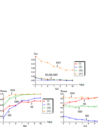
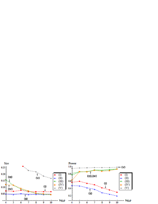
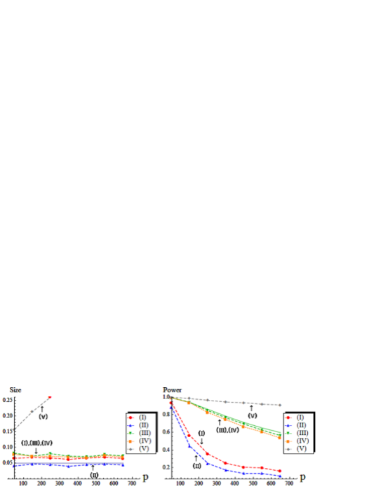
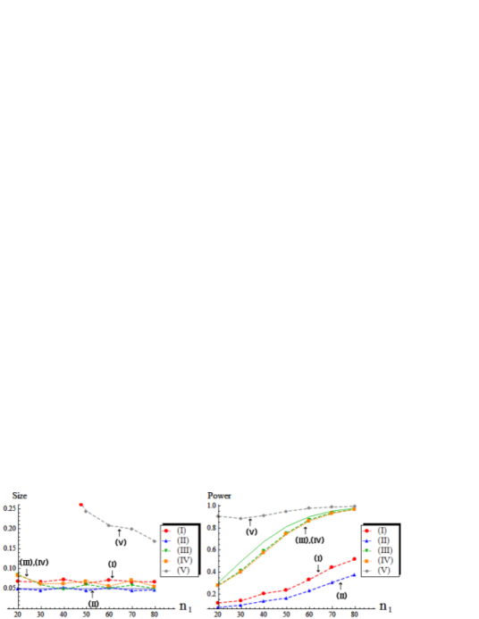
![[Uncaptioned image]](/html/1602.02491/assets/x5.png)
![[Uncaptioned image]](/html/1602.02491/assets/x6.png)
![[Uncaptioned image]](/html/1602.02491/assets/x7.png)
![[Uncaptioned image]](/html/1602.02491/assets/x8.png)
![[Uncaptioned image]](/html/1602.02491/assets/x9.png)
![[Uncaptioned image]](/html/1602.02491/assets/x10.png)
![[Uncaptioned image]](/html/1602.02491/assets/x11.png)
![[Uncaptioned image]](/html/1602.02491/assets/x12.png)
![[Uncaptioned image]](/html/1602.02491/assets/x13.png)