Universal low-energy physics in 1D strongly repulsive multi-component Fermi gases

Abstract

It was shown [Chin. Phys. Lett. 28, 020503 (2011)] that at zero temperature the ground state of the one-dimensional (1D) $w$-component Fermi gas coincides with that of the spinless Bose gas in the limit $\omega\to\infty$. This behaviour was experimentally evidenced through a quasi-1D tightly trapping ultracold ¹⁷³Yb atoms in the recent paper [Nature Physics 10, 198 (2014)]. However, understanding of low temperature behaviour of the Fermi gases with a repulsive interaction acquires spin-charge separated conformal field theories of an effective Tomonaga-Luttinger liquid and an antiferromagnetic $SU(w)$ Heisenberg spin chain. Here we analytically derive universal thermodynamics of 1D strongly repulsive fermionic gases with $SU(w)$ symmetry via the Yang-Yang thermodynamic Bethe ansatz method. The analytical free energy and magnetic properties of the systems at low temperatures in a weak magnetic field are obtained through the Wiener-Hopf method. In particular, the free energy essentially manifests the spin-charge separated conformal field theories for the high symmetry systems with arbitrary repulsive interaction strength. We also find that the sound velocity of the Fermi gases in the large $w$ limit coincides with that for the spinless Bose gas, whereas the spin velocity vanishes quickly as $w$ becomes large. This indicates a strong suppression of the Fermi exclusion statistics by the commutativity feature among the $w$-component fermions with different spin states in the Tomonaga-Luttinger liquid phase. Moreover, the equations of state and critical behaviour of physical quantities at finite temperatures are analytically derived in terms of the polylogarithm functions in the quantum critical region.

I Introduction

Advances in manipulating alkaline-earth atoms provide a promising platform for studying quantum systems with high spin symmetries Gorshkov2010NP ; Gorshkov2014NP ; Bloch2008RMP ; XWGuan2013RMP ; TLHo1998PRL ; Wu:2003 ; Bloch2012NP ; Krauser2012 ; Cazalilla2014 . The nuclear spin of most alkaline-earth isotopes is either zero or half-odd number, therefore the ultracold gases of these atoms are either single component bosons or multicomponent fermions. The electronic spins decouple from nuclear spins in alkaline-earth atoms that gives $SU(w)$ symmetry with $w=2I+1$ in two-body collisions, here $I$ is the nuclear spin. Through fully controllable interaction and spin states, a variety of high symmetry systems have been realized in the laboratories. For example, ¹⁷³Yb and ⁸⁷Sr are the alkali earth fermionic atoms which can display high spin symmetries, i.e. ¹⁷³Yb atoms have $SU(6)$ symmetry Fukuhara2007PRL ; Taie2010PRL and ⁸⁷Sr atoms have $SU(10)$ symmetry XZhang2014S . These experimental developments provide exciting opportunities to explore a wide range many-body phenomena such as spin and orbital magnetism Cappellini2014PRL ; Scazza2014NP , Kondo spin-exchange physics Nakagawa:2015 ; Zhang2015 , the synthetic dimension Zeng2015 and the one-dimensional (1D) Tomonaga-Luttinger liquid (TLL) Pagano2014NP etc.

Ultracold alkaline-atoms have opened many ways to study low-dimensional systems of interacting fermions, bosons and spins, see recent review papers YALiao2010N ; CazalillaRMP ; XWGuan2013RMP ; Murray2015 . Large spin systems of cold atoms exhibit rich internal structures which may result in multi-component quantum liquids and diverse critical phenomena XWGuan2013RMP ; Cazalilla2014 ; YCYu2015 ; Wu:2006 ; Capponi:2015 ; Schlottmann:1997 . Theoretical progress toward understanding large spin magnetism and quantum liquids was made particular on $SO(5)$ symmetry and $SU(w)$ symmetry in the scenario of alkaline-earth atoms. From the ultracold atom perspective, the integrable model of the $SU(w)$ Fermi gases, which was solved by Sutherland Sutherland1968PRL in 1968, are having high impact, see review XWGuan2013RMP . In this regard, some new integrable systems with exotic symmetries such as $SO(w)$ and $Sp(w)$ symmetries have been recently constructed by using the Bethe ansatz (BA) JPCao2007EPL ; Jiang2011JPA . So far the exact results of 1D integrable quantum systems with large symmetries have provided a better understanding of large spin magnetism, quantum liquids, universal thermodynamics and universal laws XWGuan2013RMP ; Cazalilla2014 ; YCYu2015 ; Schlottmann:1997 ; Guan2010PRA ; GuanXW2011PRA ; GuanIJMP ; Patu:2015 .

In regard of the integrability, the renewed interest over the past decade has been paid in the exactly solved models of interacting fermions and bosons. Since the pioneering work in the 60’s, 70’s and 80’s of McGuire, Yang, Lieb, Sutherland, Baxter et al., for example McGuire:1964 ; Lieb1963PR ; LiebLiniger1963PR ; Yang1967PRL ; Baxter:1972 , the understanding of integrable models has greatly extended our knowledge in the theories of many-body physics, condensed matter physics, ultracold atomic physics, quantum phase transitions and critical phenomena. The 1D many-body systems exhibit rich properties some of which might be significantly different from that of the models in higher dimensions. In particular, the hallmark of 1D many-body physics is the spin-charge separation phenomenon Giamarchi:2004 ; 1D-Hubbard ; CazalillaRMP ; Recati2003PRL ; Fuchs2005PRL ; Kollath2005PRL which does not exist in higher dimensions. In this scenario, 1D integrable quantum systems, solved by means of the BA method Lieb1963PR ; LiebLiniger1963PR ; Yang1967PRL ; Gaudin1967PLA , usually provide a rigorous proof of such unique 1D many-body phenomenon. Affleck Affleck1986 and Cardy Cardy1986 showed that conformal invariance gives a universal forms for the finite temperature and finite size effects in 1D systems. In this context, Mezincescu et al. Nepomechie1992 ; Nepomechie1993 derived the finite temperature correction in the free energy of spin chains under a small magnetic field by using the Wiener-Hopf technique, also see Schlottmann:1997 . Following these methods, analytical free energies and magnetic properties for the two- and three-component repulsive Fermi gases Lee2012PRB ; PHe2011JPA at low temperatures have been derived from the thermodynamic Bethe ansatz (TBA) equations, Yang1969JMP ; Takahashi1999 ; XWGuan2013RMP ; Schlottmann:1997 . Recently, the quantum transfer matrix method has been adapted to treat thermodynamics of the 1D interacting Bose and Fermi gases Patu:2015 ; Klumper:2011 ; Patu:2015b . Despite much theoretical study on the 1D Fermi gases in literature, rigorous derivation of such unique 1D many-body phenomenon for these high symmetry systems still has not been achieved.

In this paper, we aim to investigate universal feature of the TLL in the 1D $SU(w)$ symmetry Fermi gases with repulsive interactions by solving the TBA equations. The analytical free energy and magnetic properties of the systems at low temperatures in a weak magnetic field are derived by using the Wiener-Hopf method. At low temperatures, the free energy of the systems shows the spin-charge separated conformal field theories of an effective TLL and an antiferromagnetic $SU(w)$ Heisenberg spin chain, where the central charge in the charge sector $C_{\rm c}=1$ and the central charge in the spin sector is $C_{\rm s}=w-1$ in this weak magnetic field limit. A general relation between the magnetic field and the spin velocity under pure Zeeman splitting is obtained. We find that the sound velocity of the Fermi gases in the large $w$ limit coincides with that of the spinless Bose gas, whereas the spin velocity vanishes quickly as $w$ becomes large. This nature gives rise to a precise understanding of the experimental observation Pagano2014NP that at low temperature the $w$-component Fermi gases display the bosonic spinless liquid for a large value of $w$. Our finding is consistent with the ground state properties of the high symmetry Fermi gases which were observed in Yang:2011 ; GMW:2012 . Furthermore, we study the thermodynamics and quantum criticality of the systems beyond the regime of the Tomonaga-Luttinger liquid phase. Our result reveals the universal behaviour of interacting fermions with high symmetries in 1D.

This paper is organized as follows. In Section II, the BA equations for 1D $SU(w)$ quantum gases are presented. In Section III, the Sommerfeld expansion of TBA equations in weak magnetic field and low temperature regime is carried out. In section IV, using the Wiener-Hopf method, we obtain the low temperature free energy. In section V we discuss the spin-charge separation phenomenon. In Section VI, we discuss the TLL and critical behaviour of the strong coupling Fermi gases. Section VII is reserved as our conclusion and discussion.

II The Model and thermodynamic Bethe ansatz equations

We consider a 1D $\delta$-function interacting $w$-component fermionic system of $N$ particles with mass $m$, where the interactions between different components have the same coupling strength $g_{\rm 1D}$. The Hamiltonian of this system reads Sutherland1968PRL

$$H=-\frac{\hbar^{2}}{2m}\sum_{i=1}^{N}\frac{\partial^{2}}{\partial x_{i}^{2}}+g_{1D}\sum_{i<j}\delta(x_{i}-x_{j})+h\hat{S}_{z},$$ (1)

where $\hat{S}_{z}$ is the total spin of the $z$-direction, $\hat{S}_{z}=\sum_{r=1}^{w}[-(w+1)/2+r)]N_{r}$ and $h$ is the external magnetic field. Here $N_{r}$ is the particle number in the hyperfine state $r$. There are $w$ possible hyperfine states $|1\rangle,|2\rangle,\ldots,|w\rangle$ that the fermions can occupy. For the spin independent interactions, the number of fermions in each spin state is conserved. In the above equation, the interaction coupling constant is given by $g_{\mathrm{1D}}=-2\hbar^{2}/ma_{\mathrm{1D}}$, here $a_{\mathrm{1D}}$ is the effective scattering length in 1D Ols98 . The interaction between fermions in different spin states is repulsive when $g_{\rm 1D}>0$ and attractive when $g_{\rm 1D}<0$. Following the BA convention, we also introduce the interaction strength $c=mg_{1D}/\hbar^{2}$. From now on, we shall choose our units such that $\hbar^{2}=2m=1$ unless we particularly use the units.

The Hamiltonian (1) has the symmetry of $U(1)\times SU(w)$ when the magnetic field is absent, where $U(1)$ and $SU(w)$ are the symmetries of the charge and spin degrees of freedom, respectively. Although the Zeeman splitting breaks the $SU(w)$ symmetry, $\hat{S}_{z}$ is a conserved quantity. The model can be solved exactly via Bethe ansatz (BA) Sutherland1968PRL using the approach proposed by Yang1967PRL ; Yang1968PR . In the following calculation, we assume that the system is constrained to a line with a length $L$. The energy is given by

$$E=\sum_{j=1}^{N}k_{j}^{2},$$ (2)

where the pseudo-momenta $\left\{k_{j}\right\}$ are determined by the BA equations,

$${\rm e}^{\mathrm{i}k_{j}L}=\prod_{\ell=1}^{M_{1}}\frac{k_{j}-\lambda^{(w-1)}_{\ell}+{\rm i}\frac{c}{2}}{k_{j}-\lambda^{(w-1)}_{\ell}-{\rm i}\frac{c}{2}},j=1,\ldots,N.$$

$$\prod_{j=1}^{N}\frac{\lambda^{(w-1)}_{\ell}-k_{j}+{\rm i}\frac{c}{2}}{\lambda^{(w-1)}_{\ell}-k_{j}-{\rm i}\frac{c}{2}}\prod_{m=1}^{M_{w-2}}\frac{\lambda^{(w-1)}_{\ell}-\lambda^{(w-2)}_{m}+{\rm i}\frac{c}{2}}{\lambda^{(w-1)}_{\ell}-\lambda^{(w-2)}_{m}-{\rm i}\frac{c}{2}}$$

$$=-\prod_{\alpha=1}^{M_{w-1}}\frac{\lambda^{(w-1)}_{\ell}-\lambda^{(w-1)}_{\alpha}+\mathrm{i}c}{\lambda^{(w-1)}_{\ell}-\lambda^{(w-1)}_{\alpha}-\mathrm{i}c},\ell=1,\ldots,M_{w-1},$$

$$\prod_{j=1}^{M_{r+1}}\frac{\lambda^{(r)}_{\ell}-\lambda^{(r+1)}_{j}+{\rm i}\frac{c}{2}}{\lambda^{(r)}_{\ell}-\lambda^{(r+1)}_{j}-{\rm i}\frac{c}{2}}\prod_{m=1}^{M_{r-1}}\frac{\lambda^{(r)}_{\ell}-\lambda^{(r-1)}_{m}+{\rm i}\frac{c}{2}}{\lambda^{(r)}_{\ell}-\lambda^{(r-1)}_{m}-{\rm i}\frac{c}{2}}$$

$$=-\prod_{\alpha=1}^{M_{r}}\frac{\lambda^{(r)}_{\ell}-\lambda^{(r)}_{\alpha}+\mathrm{i}c}{\lambda^{(r)}_{\ell}-\lambda^{(r)}_{\alpha}-\mathrm{i}c},~{}~{}r=2,3,\cdots,w-2,\ell=1,\ldots,M_{r},$$

$$\prod_{j=1}^{M_{2}}\frac{\lambda^{(1)}_{\ell}-\lambda^{(2)}_{j}+{\rm i}\frac{c}{2}}{\lambda^{(1)}_{\ell}-\lambda^{(2)}_{j}-{\rm i}\frac{c}{2}}=-\prod_{\alpha=1}^{M_{1}}\frac{\lambda^{(1)}_{\ell}-\lambda^{(1)}_{\alpha}+\mathrm{i}c}{\lambda^{(1)}_{\ell}-\lambda^{(1)}_{\alpha}-\mathrm{i}c},\ell=1,\ldots,M_{1}.$$ (3)

Here $\{\lambda^{(r)}\}$, $r=1,2,\cdots,w-1$ denote the spin rapidities which are introduced to describe the motion of spin waves. The particle number $N_{r}$ in each spin state links to the quantum number $M_{\alpha}$ via the relation $N_{r}=M_{r}-M_{r-1}$ and $M_{0}=0$. In this paper, we will consider the repulsive interaction, i.e. $c>0$. There is no charged bound state for the repulsive interaction, and the pseudo-momenta $\left\{k_{j}\right\}$ are hence real. At the thermodynamic limit, i.e. $N,L\rightarrow\infty$ and $n=N/L$ is finite. Each branch of spin rapidities $\{\lambda^{(r)}\}$ has complex roots

$$\lambda^{(r)}_{q,j,z} =\lambda^{(r)}_{q,j}-\frac{\mathrm{i}c}{2}(q+1-2z),\qquad z=1,\cdots,q,$$ (4)

at the thermodynamic limit. For given $r,q$ and $j$, rapidities with different $z$ share the same real part $\lambda^{(r)}_{q,j}$, which are called $q$-string in the spin branch $r$. Here the number $q$ is the length of the string, and $j=1,2,\cdots,M^{(r)}_{q}$ label the different real parts of the $q$-strings, where $M^{(r)}_{q}$ is the number of the $q$-strings with $M^{(r)}=\sum_{q}qM^{(r)}_{q}$.

In order to carry out our calculation, we first recall some basis notations for the TBA equations. At the thermodynamic limit, the particle densities $\{\rho\}$, hole densities $\{\rho_{\rm h}\}$ are introduced to describe the equation of the state of system and the dressed energies $\varepsilon$ are defined as $\varepsilon=T\ln(\rho_{\rm h}/\rho)$. Following Yang-Yang’s grand canonical method Yang1969JMP the TBA equations for the model (1) are given by Takahashi1999 ; XWGuan2013RMP ; Schlottmann:1997 ; Lee:2011

$$\textstyle\varepsilon^{\rm c}(k) = k^{2}-\mu-sh+\sum_{n=1}^{\infty}\hat{a}_{n}\ast\varepsilon^{w-1,n}_{-},$$

$$\textstyle\varepsilon^{w-1,n}(\lambda) = nh+\hat{a}_{n}\ast\varepsilon^{\rm c}_{-}+\sum_{m}\hat{C}_{n,m}\ast\varepsilon^{w-2,m}_{-}-\sum_{m}\hat{T}_{mn}\ast\varepsilon^{w-1,m}_{-},$$

$$\textstyle\varepsilon^{r,n}(\lambda) = nh+\sum_{m}\hat{C}_{n,m}\ast(\varepsilon^{r-1,m}_{-}+\varepsilon^{r+1,m}_{-})-\sum_{m}\hat{T}_{mn}\ast\varepsilon^{r,m}_{-},$$

$$\textstyle\varepsilon^{1,n}(\lambda) = nh+\sum_{m}\hat{C}_{n,m}\ast\varepsilon^{2,m}_{-}-\sum_{m}\hat{T}_{mn}\ast\varepsilon^{1,m}_{-}.$$ (5)

Where $\varepsilon^{\rm c}(k)$ and $\varepsilon^{r,n}(k)$ are the dressed energies for the charge sector and for the branch $r$ in the spin sector, respectively and $\varepsilon_{\pm}=T\ln(1+{\rm e}^{\pm\varepsilon/T})$. As a convention used in the TBA equations, $n$ labels the length of the strings and we denote $\ast$ as the convolution integral, i.e. $\hat{a}\ast f(x)=\int_{-\infty}^{\infty}a(x-y)f(y){\rm d}y$ and the integral kernels are given by

$$a_{m}(x) = \frac{1}{2\pi}\frac{mc}{(mc/2)^{2}+x^{2}},$$

$$T_{mn} = a_{m+n}+2a_{m+n-2}+\ldots+2a_{|m-n|+2}+(1-\delta_{nm})a_{|m-n|},$$

$$C_{mn} = a_{m+n-1}+a_{m+n-3}+\ldots+a_{|m-n|+3}+a_{|m-n|+1}.$$ (6)

Using the Fourier transformation, we may rewrite the above TBA equations (II) into the following recursive form

$$\textstyle\varepsilon^{\rm c} = k^{2}-\mu+\hat{G}_{\rm c}\ast\varepsilon^{\rm c}_{-}-\sum_{r=1}^{w-1}\hat{G}_{r}\ast\varepsilon^{r,1}_{+},$$

$$\textstyle\varepsilon^{r,n} = \hat{G}\ast(\varepsilon^{r+1,n}_{+}+\varepsilon^{r-1,n}_{+}+\varepsilon^{r,n+1}_{+}+\varepsilon^{r,n-1}_{+}),$$ (7)

where $\varepsilon^{r,0}_{\pm}=\varepsilon^{0,n}_{\pm}=\varepsilon^{w,m}_{\pm}=0$ when $m>1$ and $\varepsilon^{w,1}=\varepsilon^{\rm c}$ and the integral kernels are

$$G_{r}(x) = \frac{(wc)^{-1}\sin(r\pi/w)}{\cos(r\pi/w)+\cosh(2\pi x/wc)},~{}~{}r=1,2,\cdots,w-1,$$ (8)

$$G_{\rm c} = \hat{G}_{w-1}\ast a_{1},~{}~{}~{}G(x)=\frac{1}{2c\cosh\left(\pi x/c\right)},$$ (9)

The boundary condition of these recursive equations is

$$\lim_{n\rightarrow\infty}\varepsilon^{r,n}=nh.$$ (10)

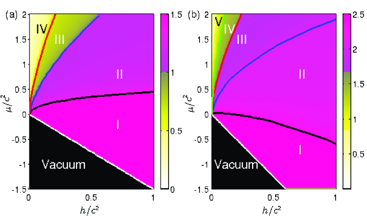
Figure 1: Phase diagram of 1D repulsive $SU(w)$ fermions: (a) The phase diagram of spin-$3/2$ model. (b) The phase diagram of spin-$5/2$ model. See the main text.

The TBA equations (II) determine full thermodynamics and critical behaviour of the 1D $SU(w)$ quantum gases. For zero temperature, i.e. $T\to 0$, the model exhibits a very rich phase diagram. In this limit, the TBA equations become the linear integral equations from which the full phase diagram can be derived analytically and numerically. When the external magnetic field $h$ is stronger than the saturation field $h_{c}=\mu/s$, the system is fully polarized to the state with spin $s_{z}=s=(w-1)/2$. For decreasing the magnetic field $h$, Zeeman splitting become weaker. Thus different branches of spin states emerge in the ground state. Solving the TBA equations (II) in the zero temperature limit, we plot the phase diagrams of the spin-$3/2$ and spin-$5/2$ Fermi gases in Fig. 1. Where phase (I) stands for the fully polarized state where $s_{z}=s$. phase (II) is the mixture of two spin states $s_{z}=s$ and $s_{z}=s-1$, phase (III) denotes the mixture of three branches where $s_{z}=s$, $s_{z}=s-1$ and $s_{z}=s-2$ and so on.

III Low temperature and weak magnetic field regime

For the ground state, i.e. $T=0$, all spin rapidities are real, thus we can denote $\varepsilon^{r,1}=\varepsilon^{r}$ for our convenience. At finite temperatures, the string solutions (complex solutions) emerge in each spin branches. Analyzing the TBA equations (II) or (II), very small numbers of strings involve in the low temperature thermodynamics. The presence of these strings make the nonlinear TBA equations very hard to be solved analytically. However, when the temperature is much smaller than magnetic field, $T\ll h$, the TBA equations of dressed energies can be simplified as

$$\varepsilon^{\rm c} = k^{2}-\mu+\hat{G}_{\rm c}\ast\varepsilon^{\rm c}_{-}-\sum_{r=1}^{w-1}\hat{G}_{r}\ast\varepsilon^{r}_{+},$$

$$\varepsilon^{r} = h+\hat{G}_{r}\ast\varepsilon^{\rm c}_{-}+\sum_{r^{\prime}}\hat{R}_{rr^{\prime}}*\varepsilon^{r^{\prime}}_{+},~{}~{}r=1,2,\cdots,w-1$$ (11)

up to ignorance of higher length strings, see the method used in Lee2012PRB ; PHe2011JPA . For the ground state, $\varepsilon^{r}(\pm\infty)\geq 0$ and $\varepsilon^{r}(0)<0$, which means $\varepsilon^{r}(k)$ has two zero points $\pm Q_{r}$ in the spin rapidity space of the $r$-branch, i.e. two Fermi like points in the spin rapidity space. For zero external magnetic field, the zero point $Q_{r}\to\infty$. For a weak magnetic field $h$, $Q_{r}$ is very large. If the magnetic field $h$ is very small, i.e. $hc\ll p$, we can use the Wiener-Hopf method to solve the second equation of (III) in spin sectors. Here the pressure is defined by

$$p=-\frac{1}{2\pi}\int_{-\infty}^{\infty}\varepsilon^{\rm c}_{-}(k){\rm d}k.$$ (12)

Before further going on, we define some convolution operators: $\circ$ is defined by $\hat{R}\circ\varepsilon(k)=\big{[}\int_{-\infty}^{-Q}+\int_{Q}^{\infty}\big{]}{\rm d}k^{\prime}R(k-k^{\prime})\varepsilon(k^{\prime})$ and $\bullet$ is defined by $\hat{R}\bullet\varepsilon(k)=\int_{-Q}^{Q}{\rm d}k^{\prime}R(k-k^{\prime})\varepsilon(k^{\prime})$. When $T\ll|\varepsilon(0)|$, we can apply Sommerfeld expansion technique to eq. (III) with the temperature $T\rightarrow 0$. We consider the leading order

$$R\ast\varepsilon_{+}(k)\approx R\circ\varepsilon(k)+R(k,Q)\xi,\,\,\,R\ast\varepsilon_{-}(k)\approx R\bullet\varepsilon-R(k,Q)\xi$$

where $R(k,Q)=R(k+Q)+R(k-Q)$ and $\xi=\pi^{2}T^{2}/6\varepsilon^{\prime}(Q)$. The equations dressed energies are thus given by

$$\varepsilon^{\rm c}=k^{2}-\mu+\hat{G}_{\rm c}\bullet\varepsilon^{\rm c}-\sum_{r=1}^{w-1}\hat{G}_{r}\circ\varepsilon^{r}-G_{\rm c}(k,Q_{\rm c})\xi_{\rm c}-\sum_{r=1}^{w-1}G_{r}(k,Q_{r})\xi_{r},$$ (13)

$$\varepsilon^{r}=h+\hat{G}_{r}\bullet\varepsilon^{\rm c}+\sum_{r^{\prime}}\hat{R}_{rr^{\prime}}\circ\varepsilon^{r^{\prime}}-G_{r}(k,Q_{\rm c})\xi_{\rm c}+\sum_{r^{\prime}}R_{rr^{\prime}}(k,Q_{r^{\prime}})\xi_{r^{\prime}}.$$

When the magnetic field is very small, the zero point $Q_{r}$ will be so large such that the quantity $z={\rm e}^{-Q_{r}\pi/c}\ll 1$. Up to the first order of $z$, we get the following asymptotic forms:

$$\hat{G}_{r}\circ\varepsilon^{r}(k)=\frac{4\sin(r\omega_{0}c)}{wc}\cosh(\omega_{0}k){\rm e}^{-{\rm i}\omega_{0}Q_{r}}\int_{0}^{\infty}{\rm d}k^{\prime}\varepsilon^{r}(k^{\prime}+Q_{r}),$$

$$\hat{R}_{rr^{\prime}}\circ\varepsilon^{r^{\prime}}(k+Q_{r^{\prime}})=\int_{0}^{\infty}{\rm d}k^{\prime}\hat{\mathds{R}}_{rr^{\prime}}(k-k^{\prime})\varepsilon^{r^{\prime}}(k^{\prime}+Q_{r^{\prime}})+O(z^{2}),$$

$$\hat{G}_{r}\bullet\varepsilon^{\rm c}(k)=b_{\varepsilon}\hat{G}_{r}(k),~{}~{}~{}~{}r,r^{\prime}=1,2,\cdots,w-1,~{}~{}~{}\omega_{0}=2\pi/wc,$$

$$b_{\varepsilon}=\hat{I}\bullet\big{[}\cosh(\omega_{0}k)\varepsilon^{\rm c}(k)\big{]},$$ (14)

where $\hat{I}$ is the convention operator of kernel $\delta(x-x^{\prime})$. Submit these results into eq. (13), we have

$$\varepsilon^{\rm c} = k^{2}-\mu+\hat{G}_{\rm c}\bullet\varepsilon^{\rm c}(k)-G_{\rm c}(k,Q_{\rm c})\xi_{\rm c}-\sum_{r=1}^{w-1}G_{r}(k,Q_{r})\xi_{r}$$ (15)

$$-\sum_{r=1}^{w-1}\frac{4\sin(r\omega_{0}c)}{wc}\cosh(\omega_{0}k){\rm e}^{-{\rm i}\omega_{0}Q_{r}}\int_{0}^{\infty}{\rm d}k^{\prime}\varepsilon^{r}(k^{\prime}+Q_{r}),$$

$$\varepsilon^{r}(k+Q_{r}) = h+b_{\varepsilon}G_{r}(k+Q_{r})+\sum_{r^{\prime}}\int_{0}^{\infty}\hat{\mathds{R}}_{rr^{\prime}}\circ\varepsilon^{r^{\prime}}(k+Q_{r^{\prime}})$$

$$-2\cosh(\omega_{0}Q_{\rm c})G_{r}(k+Q_{r})\xi_{\rm c}+\sum_{r^{\prime}}\mathds{R}_{rr^{\prime}}(k+Q_{r},Q_{r^{\prime}})\xi_{r^{\prime}}.$$

In the second equation of (15), we may take the following approximations $R_{rr^{\prime}}(k+Q_{r},Q_{r^{\prime}})\approx\mathds{R}_{rr^{\prime}}(k)$ and $G_{r}(k+Q_{r},Q_{\rm c})\approx 2\cosh(\omega_{0}c)G_{r}(k+Q_{r})$. We define functions $y_{\pm}$ as

$$y^{r}_{\pm}(k)=\theta(\pm k)\varepsilon^{r}(k+Q_{r}),$$ (16)

where $\theta(k)$ is the step function, $\theta(k)=1$ when $k>0$ and $\theta(k)=0$ when $k<0$. Submitting the function $y^{r}_{\pm}$ into the equation of $\varepsilon^{r}$, we obtain the Wiener-Hopf type equation

$$y^{r}_{+}(k)+y^{r}_{-}(k)=g_{r}(k)+\sum_{r^{\prime}}\mathds{R}_{rr^{\prime}}*y^{r}_{+}(k),$$ (17)

where $y^{r}_{+}(k)$ relates to the dressed energy $\varepsilon^{r}(k+Q_{r})$ for $k>0$. Whereas $y^{r}_{-}(k)$ is just a continuation of $y^{r}_{+}(k)$ via eq.(17). Up to the first order of $z$, the $g_{r}$ function is

$$g_{r}(k) = h+B_{\varepsilon}\hat{G}_{r}(k+Q_{r})+\sum_{r^{\prime}}\mathds{R}_{rr^{\prime}}(k)\xi_{r^{\prime}},$$ (18)

$$B_{\varepsilon} = b_{\varepsilon}-2\cosh(\omega_{0}Q_{\rm c})\xi_{\rm c}.$$ (19)

We will solve the eq. (17) to get $y^{r}_{+}(k)$ with the help of the Wiener–Hopf method next section.

For charge sector, the equation (13) can be rewritten as

$$\varepsilon^{\rm c}=k^{2}-\mu+\hat{G}_{\rm c}\bullet\varepsilon^{\rm c}(k)-G_{\rm c}(k,Q_{\rm c})\xi_{\rm c}-\sum_{r=1}^{w-1}G_{r}(k,Q_{r})\xi_{r}$$

$$\quad~{}-\sum_{r=1}^{w-1}\frac{4\sin(r\omega_{0}c/2)}{wc}\cosh(\omega_{0}k){\rm e}^{-\omega_{0}Q_{r}}\int_{0}^{\infty}{\rm d}k^{\prime}\varepsilon^{r}(k^{\prime}+Q_{r}).$$ (20)

Substituting the function $y^{r}_{+}(k)$ into the eq.(III), we further obtain

$$\varepsilon^{\rm c}\approx k^{2}-\mu+\hat{G}_{\rm c}\bullet\varepsilon^{\rm c}(k)-G_{\rm c}(k,Q_{\rm c})\xi_{\rm c}-4\cosh(\omega_{0}k)S_{\varepsilon}/wc,$$

$$S_{\varepsilon}=\sum_{r}\sin(\omega_{0}rc/2){\rm e}^{-\omega_{0}Q_{r}}\big{[}\tilde{y}_{+}({\rm i}\omega_{0})+\xi_{r}\big{]},$$ (21)

where $\tilde{y}(\omega)$ is defined by the Fourier transform

$$\tilde{f}(\omega)=\int_{-\infty}^{\infty}f(k){\rm e}^{{\rm i}k\omega}{\rm d}k.$$ (22)

IV Wiener–Hopf solution

By using the Wiener–Hopf method we will solve the eq.(17) in this section. Applying the Fourier transform (22) to eq.(17), we have

$$\tilde{y}^{r}_{+}+\tilde{y}^{r}_{-}=\tilde{g}_{r}+\sum_{r^{\prime}}\tilde{R}_{rr^{\prime}}*\tilde{y}^{r}_{+}.$$ (23)

If the functions $y^{r}_{\pm}(\pm k)$ in eq.(17) are analytic and bounded for $k>0$, $\tilde{y}_{\pm}(\omega)$ are analytic in the upper/lower half plane with the condition $\tilde{y}_{\pm}(\infty)=0$.

In the framework of Wiener-Hopf method, the integral kernels $(1-R)^{-1}$ must be factorized into two functions which are analytic in upper/lower half plane. However, the Eq.(23) is difficult to solve for the case that $R$ is a matrix. The $R$ can be diagonalized by using the transformation matrix

$$U_{rr^{\prime}}=\sqrt{\frac{2}{w}}\sin\frac{rr^{\prime}\pi}{w},$$ (24)

where $U$ is a unitary matrix, $UU=1,U=U^{-1},U=U^{t},U=U^{\dagger}$. Making the following transformation,

$$\textstyle\bar{y}^{r}_{\pm}=\sum_{r^{\prime}}U_{rr^{\prime}}\tilde{y}^{r}_{\pm},~{}\bar{g}_{r}=\sum_{r^{\prime}}U_{rr^{\prime}}\tilde{g}_{r},~{}\bar{R}_{r}\delta_{rr^{\prime}}=\sum_{r_{1}r_{2}}U_{rr_{1}}\tilde{R}_{r_{1}r_{2}}U_{r_{2}r^{\prime}},$$ (25)

$$(1-\bar{R}_{r})^{-1}=4\tilde{a}_{1}\cosh\Big{[}\frac{\omega c}{4}-\frac{\pi{\rm i}}{2}\frac{r-w}{w}\Big{]}\cosh\Big{[}\frac{\omega c}{4}+\frac{\pi{\rm i}}{2}\frac{r-w}{w}\Big{]},$$

we then obtain the diagonalized Wiener-Hopf equation

$$\textstyle\bar{y}^{r}_{-}=\bar{g}_{r}+\bar{R}_{r}\bar{y}^{r}_{+},$$ (26)

As usual Lee2012PRB ; PHe2011JPA , the term $(1-\bar{R}_{r})^{-1}$ can be decomposed into two parts, $\bar{K}^{r}_{+}(\omega)$ and $\bar{K}^{r}_{-}(\omega)$, namely

$$(1-\bar{R}_{r})^{-1}=\bar{K}^{r}_{+}\bar{K}^{r}_{-},$$ (27)

where $\bar{K}^{r}_{\pm}(\omega)$ are analytic and nonzero in the upper/lower half-plane with the properties $\bar{K}^{r}_{+}(\omega)=\bar{K}^{r}_{-}(-\omega)$ and the term $\bar{K}^{r}_{\pm}(\omega)|_{|\omega|\to\infty}=1$. Finally, the eq.(26) can be decomposed into the following form

$${\bar{y}^{r}_{+}}/{\bar{K}^{r}_{+}}=\bar{K}^{r}_{-}\bar{g}_{r}-\bar{K}^{r}_{-}\bar{y}^{r}_{-}.$$ (28)

Here, term $\bar{y}^{r}_{+}/{\bar{K}^{r}_{+}}$ is analytic in the upper half-plane and term $\bar{K}^{r}_{-}\bar{y}^{r}_{-}$ is analytic in the lower half-plane.

We assume that $\bar{K}^{r}_{-}\bar{g}_{r}$ can be further decomposed into two parts

$$\bar{K}^{r}_{-}\bar{g}_{r}=\bar{\varPhi}^{r}_{+}+\bar{\varPhi}^{r}_{-},$$ (29)

where $\bar{\varPhi}^{r}_{+}$ and $\bar{\varPhi}^{r}_{-}$ are analytic in the upper and lower half-plane, respectively. From this equation, we can get

$${\bar{y}^{r}_{+}}/{\bar{K}^{r}_{+}}-\bar{\varPhi}^{r}_{+}=\bar{\varPhi}^{r}_{-}-\bar{K}^{r}_{-}\bar{y}^{r}_{-}.$$ (30)

In the eq.(30), the left and right hand sides are analytic and bounded in the upper and lower half-planes, respectively. From Liouville’s theorem, both sides of eq.(30) should be a constant. When $\omega\to\infty$, $\bar{y}^{r}_{+}\to 0$ and $\bar{K}^{r}_{\pm}\to 1$. This provides us a way to determine this constant and leads to the solution of $\bar{y}^{r}_{+}$ in the form

$${\bar{y}^{r}_{+}}(\omega)={\bar{K}^{r}_{+}}(\omega)[\bar{\varPhi}^{r}_{+}(\omega)-\bar{\varPhi}^{r}_{+}(\infty)].$$ (31)

With the help of the relations ${\rm e}^{-|\omega|a}=[\alpha/(\epsilon-{\rm i}\omega)]^{{\rm i}\omega a/\pi}[\alpha/(\epsilon+{\rm i}\omega)]^{-{\rm i}\omega a/\pi}$ and $2\cosh\omega a=\sqrt{2\pi}\Gamma(1/2+{\rm i}\omega a/\pi)^{-1}\Gamma(1/2-{\rm i}\omega a/\pi)^{-1}$ where $\epsilon=0^{+}$ is infinitely small and $\alpha$ is a constant. Then the factorization of $(1-\bar{R}_{r})^{-1}$ is given by

$$\bar{K}^{r}_{\pm}(\pm\omega)=2\pi\Gamma\Big{(}\frac{r}{2w}-\frac{{\rm i}\omega c}{4\pi}\Big{)}^{-1}\Gamma\Big{(}1-\frac{r}{2w}-\frac{{\rm i}\omega c}{4\pi}\Big{)}^{-1}\Big{(}\frac{4\pi{\rm e}/c}{\epsilon-{\rm i}\omega c}\Big{)}^{\frac{{\rm i}\omega c}{2\pi}}.$$ (32)

The functions $\bar{K}^{r}_{\pm}$ is analytic and nonzero in the upper/lower half-plane. The condition $\bar{K}^{r}_{\pm}(\infty)=1$ can be seen from the asymptotic form of $\bar{K}^{r}_{+}$ for a large $\omega$:

$$\bar{K}^{r}_{+}(\omega)|_{|\omega c|\gg 1}=1-\alpha_{0}\frac{2\pi}{{\rm i\omega c}}+\frac{\alpha_{0}^{2}}{2}\Big{(}2\frac{\pi}{{\rm i\omega c}}\Big{)}^{2}+O(\omega^{-3}),$$ (33)

where $\alpha_{0}=-1/3+r(1-r/2w)/w$. In the lower/upper half plane, the poles of $\bar{K}_{\pm}$ are at $\mp\omega_{m}$ where $\omega_{m}=2m\pi{\rm i}/wc,m=1,2,\cdots$.

From the functions $\bar{K}^{r}_{-}$ given in eq. (32) and $g_{r}(k)$ given in eq. (18), we may decompose $\bar{K}^{r}_{-}\bar{g}_{r}$. Following Lee2012PRB , then the $\bar{\varPhi}^{r}_{+}$ is given by

$$\bar{\varPhi}^{r}_{+}(\omega) =\frac{{\rm i}\bar{h}_{r}\bar{K}^{r}_{+}(0)}{\omega+{\rm i}\epsilon}-\frac{2{\rm i}B_{\varepsilon}}{wc}\sum_{m=0}^{\infty}\frac{(-1)^{m}\bar{K}_{+}(\omega_{m})\bar{J}_{m}}{\omega+\omega_{m}}+\bar{K}_{+}(\omega)\bar{\xi}_{r}-\bar{\xi}_{r},$$

$$\bar{J}_{m} =-\sum_{r^{\prime}}U_{rr^{\prime}}{\rm e}^{{\rm i}\omega_{m}Q_{r^{\prime}}}\sin({\rm i}\omega_{m}r^{\prime}c/2).$$ (34)

Where $\bar{h}_{r}=h\sum_{r^{\prime}}U_{rr^{\prime}}$, $\epsilon$ is a infinitely small value and $\epsilon>0$. By using the exact form of $\bar{\varPhi}^{r}_{+}$, the function $\bar{y}^{r}_{+}$ is given by

$$\bar{y}^{r}_{+} =\bar{K}^{r}_{+}\Big{[}\frac{{\rm i}\bar{h}_{r}\bar{K}^{r}_{+}(0)}{\omega+{\rm i}\epsilon}-\frac{2{\rm i}B_{\varepsilon}}{wc}\sum_{m}\frac{(-1)^{m}\bar{K}^{r}_{+}(\omega_{m})\bar{J}^{r}_{m}}{\omega+\omega_{m}}\Big{]}+({\bar{K}^{r}_{+}}-1)\bar{\xi}_{r}.$$ (35)

It is obviously that $\bar{y}^{r}_{+}$ is analytic in the upper half-plane. The poles in the lower half plane are located at positions $\omega=-{\rm i}\epsilon$ and $\omega_{-m}$, $m=1,2,\cdots$. With the large $\omega$ asymptotic form of $\bar{K}^{r}_{+}$, the function $\bar{y}^{r}_{+}$ can be expanded to

$$\bar{y}^{r}_{+}(\omega)=\bar{\sigma}_{1}\frac{2\pi}{{\rm i}\omega c}+\bar{\sigma}_{2}\Big{(}\frac{2\pi}{{\rm i}\omega c}\Big{)}^{2}+O(\omega^{-3}).$$ (36)

where $|\omega|\gg 1$ and

$$\bar{\sigma}^{r}_{1}=-\frac{\bar{h}_{r}c}{2\pi}\bar{K}^{r}_{+}(0)+\frac{b_{\varepsilon}}{w\pi}\sum_{m}(-1)^{m}K^{r}_{+}(\omega_{m})\bar{J}_{m}-\alpha_{0}\bar{\xi}_{r},$$

$$\bar{\sigma}^{r}_{2}=\alpha_{0}\frac{\bar{h}_{r}c}{2\pi}\bar{K}^{r}_{+}(0)-\frac{2b_{\varepsilon}}{w\pi}\sum_{m}(-1)^{m}K^{r}_{+}(\omega_{m})\bar{J}_{m}(\frac{{\rm i}\omega_{m}c}{2\pi}+\alpha_{0})+\alpha_{0}^{2}\bar{\xi}_{r}/2,$$

The value $y_{+}(\infty)$ is determined from $y^{r}_{+}(\infty)=-{\rm i}\,{\rm Res}[\tilde{y}^{r}(0)]=\sum_{r^{\prime}}U_{rr^{\prime}}\bar{K}_{r^{\prime}}(0)^{2}\bar{h}_{r^{\prime}}=h$, which is consistent with the boundary conditions from the thermodynamic Bethe ansatz equations. The other two boundary conditions are $y^{r}_{+}(0)=-{\rm i}{\rm Res}[\tilde{y}^{r}_{+}(\infty)]=-2\pi\sigma^{r}_{1}/c$ and $y^{\prime}_{+}(0)=-{\rm Res}[\omega\tilde{y}^{r}_{+}(\omega)|_{\omega=\infty}]=(2\pi)^{2}\sigma^{r}_{2}/c^{2}$. We further calculate $S_{\varepsilon}$ introduced in (III), i.e.

$$S_{\varepsilon}=\sum_{r}\bar{J}_{1}^{r}\Big{[}\bar{y}^{r}_{+}({\rm i}\omega_{0})+\bar{\xi}_{r}\Big{]}.$$ (37)

When $hc\ll p$, we have

$$S_{\varepsilon} = \frac{\pi}{2B_{\epsilon}(\omega_{1}^{2})}\Big{[}\frac{w(w^{2}-1)}{12}h^{2}+\frac{2}{3}{\pi^{2}T^{2}}\Big{]}.$$ (38)

Then we obtain the low temperature dressed energy $\varepsilon^{\rm c}$

$$\varepsilon^{\rm c}=k^{2}-\mu+\alpha b_{\varepsilon}^{-1}\cosh(\omega_{0}k)-G_{\rm c}(k,Q_{\rm c})\xi_{\rm c}+\hat{G}_{\rm c}\bullet\varepsilon^{\rm c}(k)$$ (39)

$$\alpha=\frac{wc}{2\pi}\Big{[}\frac{w(w^{2}-1)}{12}h^{2}+\frac{w-1}{3}{\pi^{2}T^{2}}\Big{]}.$$ (40)

Using these equations, we will calculate the exact result of low temperature behaviour for the 1D repulsive Fermi gases with a weak magnetic field.

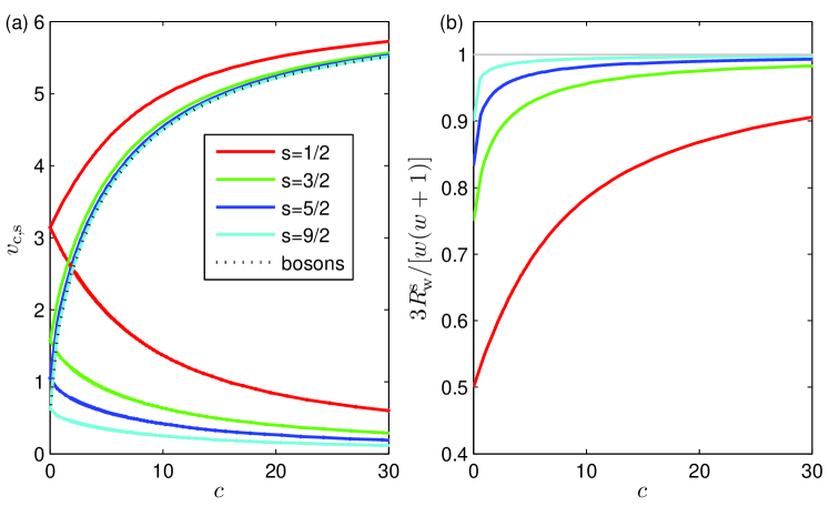
Figure 2: Spin and charge velocities and Wilson ratio for the pseudo spin-$1/2$, -$3/2$ -$5/2$ and $-9/2$ Fermi gases in weak magnetic field limit, where $h=0$ and $n=1$. (a) The velocities for the charge (upper branch) and the spin (lower branches) degrees of freedom. (b) The Wilson ratio vs interacting strength $c$ for different spin symmetries. It displays a plateaus of the height $w(w+1)/3$ in the large $w$ limit.

V Spin charge separation and low temperature behaviour

V.1 Spin-charge separation for $SU(w)$ Fermi gases

At zero temperature, the repulsive $SU(w)$ Fermi gas exhibit an antiferromagnetic ground state. At low temperatures, spin-charge separation behavior naturally occurs in TLL regime. The characteristic of the TLL for this model can be found from the simplified TBA equations (39). The eq.(39) was given in terms of the chemical potential $\mu$, the zero dressed energy point $Q_{\rm c}$ at low temperatures and the weak magnetic field $h$. At $T=0$ and $h=0$, the pseudo-Fermi point is denoted as $Q_{0}$. The integral BA equation in the charge sector is given by

$$\rho^{\rm c}_{0}(k)=\frac{1}{2\pi}+G_{\rm c}|_{Q_{0}}\bullet\rho_{0}^{\rm c}(k),$$ (41)

where the corresponding dressed energy is denoted as $\varepsilon^{\rm c}_{0}(k)$ and the corresponding pressure $p_{0}(\mu)$ only depends on the chemical potential. In low temperature limit, $|Q-Q_{0}|$ is very small and so is their energy difference $\Delta\varepsilon^{\rm c}=\varepsilon^{\rm c}-\varepsilon^{\rm c}_{0}$, here $\varepsilon^{\rm c}_{0}(Q_{0})=0$. Up to the leading order, $\Delta\varepsilon^{\rm c}$ satisfies the following equation

$$\Delta\varepsilon^{\rm c}=\alpha b_{\varepsilon}^{-1}\cosh(\omega_{0}k)-G_{\rm c}(k,Q_{\rm c})\xi_{\rm c}+\hat{G}_{\rm c}|_{Q_{0}}\bullet\Delta\varepsilon^{\rm c}(k).$$ (42)

We also can calculate the pressure via $p=p_{0}-\hat{I}\bullet\Delta\varepsilon^{\rm c}/2\pi+\xi_{c}/\pi$. Using eqs. (41) and (42), we have

$$p = p_{0}(\mu)-\alpha\frac{b_{\rho}(\mu)}{b_{\varepsilon}(\mu)}+2\xi_{\rm c}\rho_{0}(Q_{0})=p_{0}(\mu)+\Delta_{h}(\mu)h^{2}+\Delta_{T}(\mu)T^{2},~{}~{}$$ (43)

$$\Delta_{h}(\mu) = -\frac{w^{2}(w^{2}-1)c}{24\pi}\frac{b_{\rho}}{b_{\varepsilon}}=\frac{w(w^{2}-1)}{24\pi v_{\rm s}},$$ (44)

$$\Delta_{T}(\mu) = \frac{\pi^{2}}{3}\Big{[}\frac{\rho_{0}(Q_{0})}{\varepsilon^{\prime}(Q_{0})}-\frac{wc}{2\pi}(w-1)\frac{b_{\rho}}{b_{\varepsilon}}\Big{]}=\frac{\pi}{6}\Big{[}\frac{1}{v_{\rm c}}+\frac{w-1}{v_{\rm s}}\Big{]},$$ (45)

where $b_{\rho}=\hat{I}\bullet[\cosh(\omega_{0}k)\rho^{\rm c}(k)]$ and

$$v_{\rm s}=\frac{\varepsilon^{r}(Q_{r})^{\prime}}{2\pi\rho^{r}(Q_{r})}=-\frac{b_{\varepsilon}}{b_{\rho}wc},~{}~{}~{}v_{\rm c}=\frac{\varepsilon^{\rm c}(Q_{\rm c})^{\prime}}{2\pi\rho^{\rm c}(Q_{\rm c})}$$ (46)

are the pseudo Fermi velocities in the spin and charge sectors, respectively. We would like to addressed that the result eq. (43)–(45) are derived for the first time and valid for arbitrary interaction strength. Here the spin velocity $v_{\rm s}=-{b_{\varepsilon}}/({b_{\rho}wc})$ can be calculated from eq.(39) with the help of the Wiener–Hopf solution to the density. Similarly, using the Wiener–Hopf solution for the charged density, one can also reach a close form of the sound velocity $v_{\rm c}$. In the limit $h\to 0$, Hamiltonian (1) exhibits the $SU(w)$ symmetry. Therefore all the spin velocities of $w-1$ branches are the same under the pure Zeeman splitting. This means that the spin velocity $v_{\rm s}$ in eq. (46) is independent of the spin rapidity index ‘$r$’. In fact, this property holds for unequal spacing weak Zeeman splittings.

For a weak magnetic field, the density of magnetization and susceptibility are directly reached from eq. (43)

$$m_{z}=\partial_{h}p=2\Delta_{h}h,~{}~{}\chi=\partial_{h}m_{z}=2\Delta_{h}=\frac{w(w^{2}-1)}{12\pi v_{\rm s}}.$$ (47)

The magnetization linearly responds to the weak external magnetic field with a finite susceptibility. The susceptibility solely depends on the pseudo spin velocity that presents a universal feature of spin fluctuations. It is obvious to see that

$$\chi v_{\rm s}={w(w^{2}-1)}/{12\pi}.$$ (48)

This provide a universal relation between the multicomponent spin velocity and magnetic susceptibility. This relation is important to be confirmed in experiment with ultracold fermionic atoms Pagano2014NP . We observed from the FIG. 2 (a) that spin velocity decreases quickly as we increase the number of components. This means that any spin flipping process involves all spin states. In this sense, the spin transportation is strongly suppressed for a large number of spin states. From FIG. 2 (a), we also observe that for the large spin system the pseudo charge velocities turns to the pseudo charged velocity of spinless bosonic gas. This nature agrees with the experimental observation Pagano2014NP that the repulsive fermionic gases with $SU(w)$ symmetry exhibit the bosonic spinless liquid for a large value of $w$ at $T=0$ and $h=0$.

From eq. (43), the density of entropy and the specific heat

$$s_{\rm e}=\partial_{T}p=2\Delta_{T}T,~{}~{}c_{L}=T\partial_{T}s_{\rm e}=2T\Delta_{T}=\frac{\pi T}{3}\Big{[}\frac{C_{\rm c}}{v_{\rm c}}+\frac{C_{\rm s}}{v_{\rm s}}\Big{]},$$ (49)

where $C_{\rm c}=1$ and $C_{\rm s}=w-1$ are the central charges in the charge and spin sectors, respectively. The low energy properties are uniquely determined by the collective excitations in spin and charge degrees of freedom. This nature is called spin-charge separation that is a hallmark of the TLL. In the TLL phase, both quantum fluctuation and thermal fluctuation are on equal footing in regard to the temperature. The dimensionless Wilson ratio between the susceptibility and the specific heat divided by the temperature $T$,

$$R^{\rm s}_{\rm w}=\frac{4}{3}\pi^{2}\frac{\chi}{c_{\rm L}/T}=\frac{\pi v_{\rm c}w(w^{2}-1)}{3[{C_{\rm c}}{v_{\rm s}}+{C_{\rm s}}{v_{\rm c}}]},$$ (50)

measures ratio between the magnetic fluctuation and the thermal fluctuation Wil75 ; Wan98 ; XWGuan2013PRL . We plot the Wilson ratio against interaction strength for the TLL phase in FIG. 2 (b). This dimensionless ratio displaying plateaus of height $w(w+1)/3$ in the large $w$ limit, hence it captures the spin degeneracy YCYu2015 .

V.2 Universality of spin charge separation in quantum gases

As being discussed in the last section, spin charge separation is one of the most important features of the TLL. Since the TLL behavior is the typical nature of 1D quantum gases at low temperatures, the spin-charge separation may exist not only in the weak magnetic field regime but also in a high magnetic field. This fact is in general true for the integrable quantum gases, for example $SU(w)$, $Sp(w)$, $SO(w)$ symmetry quantum gases and other models. For the 1D integrable quantum Fermi gases with different high symmetries than the $SU(w)$, for example, the $SO(4)$ Fermi gas Jiang2015 , the low energy spin excitations can be spinon excitations. In general, their TBA equations can be written as

$$\varepsilon^{{\rm c},\alpha}=\tau_{\alpha}k^{2}-\mu_{\alpha}+\sum_{\beta}\hat{K}^{{\rm c},\alpha}_{{\rm c},\beta}*\varepsilon^{{\rm c},\beta}_{-}+\sum_{n}\hat{K}^{{\rm c},\alpha}_{{\rm s},n}*\varepsilon^{{\rm s},n}_{-},$$

$$\varepsilon^{{\rm s},n}=h_{n}+\sum_{\alpha}\hat{K}^{{\rm s},n}_{{\rm c},\alpha}*\varepsilon^{{\rm c},\alpha}_{-}+\sum_{m}\hat{K}^{{\rm s},n}_{{\rm s},m}*\varepsilon^{{\rm s},m}_{-}.$$ (51)

Where $\tau_{\alpha}$ is the single particle dispersion coefficients. The integral kernels satisfy $K^{a,b}_{c,d}=K^{c,d}_{a,b}$. In order to discuss the low temperature properties, we denote the dressed energies at $T=0$ as $\varepsilon_{0}$, and $\Delta\varepsilon=\varepsilon-\varepsilon_{0}$. With the help of the Sommerfeld expansion technique, we have

$$\Delta\varepsilon^{{\rm c},\alpha}= -\sum_{\beta}K^{{\rm c},\alpha}_{{\rm c},\beta}(k,Q_{{\rm c},\beta})\xi_{{\rm c},\beta}-\sum_{n}K^{{\rm c},\alpha}_{{\rm s},n}(k,Q_{{\rm s},n})\xi_{{\rm s},n}$$

$$+\sum_{\beta}\hat{K}^{{\rm c},\alpha}_{{\rm c},\beta}\bullet\Delta\varepsilon^{{\rm c},\beta}+\sum_{n}\hat{K}^{{\rm c},\alpha}_{{\rm s},n}\bullet\Delta\varepsilon^{{\rm s},n}$$

$$\Delta\varepsilon^{{\rm s},n}= -\sum_{\alpha}K^{{\rm s},n}_{{\rm c},\alpha}(k,Q_{{\rm c},\alpha})\xi_{{\rm c},\alpha}-\sum_{m}K^{{\rm s},n}_{{\rm s},m}(k,Q_{{\rm s},m})\xi_{{\rm s},m}$$

$$+\sum_{\alpha}\hat{K}^{{\rm s},n}_{{\rm c},\alpha}\bullet\varepsilon^{{\rm c},\alpha}_{-}+\sum_{m}\hat{K}^{{\rm s},n}_{{\rm s},m}\bullet\varepsilon^{{\rm s},m}.$$ (52)

At the ground state when magnetic field $h=0$, the integral TBA equations of string densities are

$$\rho_{0}^{{\rm c},\alpha}= \frac{\tau_{\alpha}}{2\pi}+\sum_{\beta}\hat{K}^{{\rm c},\alpha}_{{\rm c},\beta}\bullet\rho_{0}^{{\rm c},\beta}+\sum_{n}\hat{K}^{{\rm c},\alpha}_{{\rm s},n}\bullet\rho_{0}^{{\rm s},n}$$

$$\rho_{0}^{{\rm s},n}= \sum_{\alpha}\hat{K}^{{\rm s},n}_{{\rm c},\alpha}\bullet\rho_{0}^{{\rm c},\alpha}+\sum_{m}\hat{K}^{{\rm s},n}_{{\rm s},m}\bullet\rho_{0}^{{\rm s},m},$$ (53)

where $\mu$ is the chemical potential. From eq. (V.2) and (V.2), we can find that

$$\sum_{\alpha}\frac{\tau_{\alpha}}{2\pi}\hat{I}\bullet\Delta\varepsilon^{{\rm c},\alpha} =\frac{\tau_{\alpha}}{\pi}\sum_{\alpha}\xi_{{\rm c},\alpha}-2\sum_{\alpha}\xi_{{\rm c},a}\rho^{{\rm c},\alpha}(Q_{{\rm c},\alpha})-2\sum_{n}\xi_{{\rm s},n}\rho^{{\rm s},n}(Q_{{\rm s},n})$$

$$=\frac{\tau_{\alpha}}{\pi}\sum_{\alpha}\xi_{{\rm c},\alpha}-\frac{\pi T^{2}}{6}\Big{[}\sum_{a}\frac{1}{v_{{\rm c},\alpha}}+\sum_{n}\frac{1}{v_{{\rm s},n}}\Big{]}.$$

Up to the order of $T^{2}$, the pressure is expanded as

$$p =-\sum_{\alpha}\frac{\tau_{\alpha}}{2\pi}\hat{I}*\varepsilon^{{\rm c},\alpha}_{-}=p_{0}(\mu,h)-\sum_{\alpha}\frac{\tau_{\alpha}}{2\pi}\hat{I}\bullet\Delta\varepsilon^{\rm c,\alpha}+\sum_{\alpha}\frac{\xi_{\rm c,\alpha}}{\pi}$$

$$=p_{0}(\mu,h)+\frac{\pi T^{2}}{6}\Big{[}\sum_{a}\frac{1}{v_{{\rm c},\alpha}}+\sum_{n}\frac{1}{v_{{\rm s},n}}\Big{]}.$$ (54)

The specific heat at low temperatures is given by

$$c_{L}=\frac{\pi T}{3}\sum_{r}\frac{C_{r}}{v_{r}},~{}~{}~{}C_{r}=1.$$ (55)

where the sum is carried out over all the velocities for the charge sector and spin-wave velocities in the spin sector. The central charge for each branch of the spin degrees of freedom is $C_{r}=1$. Here the discussion does not depend on the condition that the magnetic field is weak or strong.

VI Equation of state for a strong repulsion

In fact the TBA equation of dressed energy eq. (II) or (39) can be written as

$$\varepsilon^{\rm c}=k^{2}-\mu+f(k)+\hat{G}_{\rm c}*\varepsilon^{\rm c}(k),$$ (56)

where the function $f(k)$ is the contributions from spin strings. Here the argument is general true for interacting fermions with high symmetries. When $h\gg T$, the contribution from high spin strings is very small and thus $f(k)=\alpha/b_{\varepsilon}+O(T^{2}/c\mu^{3/2},h^{2}/c\mu^{3/2})\approx f_{h\gg T}=-3\alpha\mu^{-3/2}/4$ can be analytically calculated for TLL regime, also see the attractive case Guan2010PRA . When the external field is very weak, i.e., $h\ll T$, we can find that all the high strings contribute to the pressure, i.e. $f(k)\approx f_{h\ll T}=-T\sinh(wh/2T)/\sinh(h/2T)$ for quantum criticality regime. At the strong coupling limit, we expand the following functions which are used in eq. (39)

$$G_{\rm c}(k)=\sum_{n=0}^{\infty}\frac{g_{2n}}{c^{2n+1}\pi}k^{2n},~{}~{}g_{2n}=\frac{(-1)^{n}}{w^{2n+1}}\Big{[}\zeta_{2n+1}(1/w)-\zeta_{2n+1}(0)\Big{]}.$$ (57)

Here $\zeta(x)$ is the Riemann $\zeta$ function. Then the TBA equation is expanded as

$$\varepsilon^{{\rm c}}(k) = \tau k^{2}-A+O(c^{-5},z^{2}),~{}~{}\tau=1-2g_{2}p/c^{3},$$ (58)

$$A = \mu-f_{T}+\frac{2g_{0}}{c}p-\frac{g_{2}}{c^{3}\pi}\int k^{\prime 2}\varepsilon^{\rm c}_{-}(k^{\prime}){\rm d}k^{\prime}.$$ (59)

In the above equations we calculated $-\int k^{2n}T\ln\big{[}1+{\rm e}^{-\frac{\tau k^{2}-A}{T}}\big{]}{\rm d}k={2\Gamma(n+\frac{3}{2})}T^{n+\frac{3}{2}}{\rm Li}_{n+\frac{3}{2}}\big{[}-{\rm e}^{-A/T}\big{]}/[(2n+1)\tau^{n+1/2}]=-2\Gamma(n+\frac{3}{2})T^{n+\frac{3}{2}}F_{n+\frac{1}{2}}\big{(}\frac{A}{T}\big{)}/[(2n+1)\tau^{n+\frac{1}{2}}]$, $\Gamma(5/2)={3\sqrt{\pi}}/4,~{}\Gamma(3/2)={\sqrt{\pi}}/2$, and $\int k^{\prime 2}\varepsilon^{\rm c}_{-}(k){\rm d}k=-\frac{\sqrt{\pi}}{2}\frac{T^{5/2}}{\tau^{3/2}}{F}_{3/2}(A/T)$. In the above equation, $f_{T}=f_{h\gg T}$ for the TLL phase whereas, $f_{T}=f_{h\ll T}$ for the quantum critical regime. Finally, we obtain the approximation result of the equation of state

$$p=\frac{\tau^{1/2}}{2\pi^{1/2}}T^{3/2}F_{1/2}\Big{(}\frac{A}{T}\Big{)}+O(c^{-5}),$$ (60)

$$A=\mu-f_{T}+\frac{2g_{0}}{c}p+\frac{g_{2}}{c^{3}}\frac{T^{5/2}}{2\pi^{1/2}\tau^{3/2}}F_{3/2}(A/T).$$ (61)

This serves as the equation of state which describes the exact low temperature thermodynamics of the system for the TLL and quantum critical regime, i.e. for the regions $h\ll T$ and $h\gg T$, respectively.

In the limit $h\gg T$, we find that the Fermi-Dirac integral of eq. (60) describes the low temperature behavior of the TLL. In the strong coupling limit, the charge and spin velocities are given by

$$v_{\rm c}=2\pi n(1-4g_{0}n/c),~{}~{}v_{\rm s}=\frac{4\pi^{3}n^{2}}{3wc}(1-6g_{0}n/c),$$ (62)

respectively. Where $g_{0}=\frac{1}{w}\left(\zeta(\frac{1}{w}-\zeta(0)\right)$. The susceptibility and the specific heat are

$$\chi=\frac{w^{2}(w^{2}-1)}{16\pi^{4}n^{2}}(1+6g_{0}n/c),$$

$$\frac{c_{\rm L}}{T}=\frac{w(w-1)}{4\pi^{2}n^{2}}(1+6g_{0}n/c+2\pi^{2}n/[3w(w-1)c]).$$ (63)

The Wilson ratio $R^{\rm s}_{\rm w}$ at the strong coupling limit can be expanded as

$$R^{\rm s}_{\rm w}=\frac{w(w+1)}{3}\Big{[}1-\frac{2\pi^{2}n}{3w(w-1)c}\Big{]},$$ (64)

see FIG. 2 (b). However, for weak coupling limit $c\to 0$, we can find that

$$v_{\rm s}=\frac{2\pi n}{w},~{}~{}~{}\chi=\frac{w^{2}(w^{2}-1)}{24n\pi^{2}},~{}~{}\frac{c_{\rm L}}{T}=\frac{w^{2}}{6n},~{}~{}R^{\rm s}_{\rm w}=\frac{2}{3}w(w-1).$$ (65)

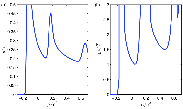
Figure 3: The low temperature behavior of compressibility and specific heat for the spin-$3/2$ Fermi gas at $T=0.005c^{2}$ and $h=0.1c^{2}$. (a) The dimensionless compressibility. (b) The dimensions specific heat. The round peaks the quantum critical behaviour near the critical point, see a similar analysis in GuanXW2011PRA .

The compressibility $\kappa^{*}$, susceptibility $\chi$ and specific heat $c_{\rm L}$ are divergent at the critical points, see FIG. 3 (a) for compressibility and FIG. 3 (b) for specific heat, respectively. These functions have singularities at the critical points and they show universal scaling behavior in the critical regions. In the quantum critical regime near the phase transition from vacuum state to the ferromagnetic state, the eq. (56) and $f(k)=-T\sinh(wh/2T)/\sinh(h/2T)$ give rise to the quantum criticality. The equation of state is given by

$$p=\frac{T^{3/2}}{2\sqrt{\pi}}F_{1/2}\Big{(}\frac{A}{T}\Big{)},~{}~{}~{}\frac{A}{T}=\frac{\mu}{T}+\ln\frac{\sinh(wh/2T)}{\sinh(h/2T)}.$$ (66)

It is clear that the the universal scaling function of the pressure is the Fermi-Dirac integral $F_{1/2}$. In the quantum critical regime, $h/T\ll 1$, thus we have $A/T\approx\ln w+\mu/T+(w^{2}-1)h^{2}/(24T^{2})$. Explicitly we have

$$n = \frac{T^{1/2}}{2\pi^{1/2}}F_{-1/2},~{}~{}~{}\kappa^{*}=\frac{T^{-1/2}}{2\pi^{1/2}}F_{-1/2},$$ (67)

$$m = \frac{T^{1/2}}{24\pi^{1/2}}(w^{2}-1)\frac{h}{T}F_{-1/2},$$ (68)

$$\chi = \frac{T^{-1/2}}{24\pi^{1/2}}(w^{2}-1)\Big{[}F_{-1/2}+\frac{w^{2}-1}{12}\frac{h^{2}}{T^{2}}F_{-3/2}\Big{]},$$ (69)

$$s = \frac{T^{1/2}}{2\pi^{1/2}}\Big{[}\frac{3}{2}F_{1/2}-\Big{(}\frac{\mu}{T}+\frac{w^{2}-1}{12}\frac{h^{2}}{T^{2}}\Big{)}F_{-1/2}\Big{]},$$ (70)

$$\frac{c_{\rm L}}{T} = \frac{T^{-1/2}}{2\pi^{1/2}}\Big{[}\frac{3}{4}F_{1/2}-\frac{\mu}{T}F_{-1/2}+\Big{(}\frac{\mu}{T}+\frac{w^{2}-1}{12}\frac{h^{2}}{T^{2}}\Big{)}^{2}F_{-3/2}\Big{]},$$ (71)

where $F_{a}=F_{a}(A/T)$ is the Fermi-Dirac integral.

VII Conclusion

We have studied the universal low temperature behaviour of the 1D interacting fermions with $SU(w)$ symmetry via the TBA method. We have developed an analytical method to obtain the pressure in terms of charge and spin velocities for the system with arbitrary interaction strength, see (43)-(49) and (54). The low temperature behaviour of these gases which we have obtained shows a universal spin-charge separated conformal field theories of an effective Tomonaga-Luttinger liquid and an antiferromagnetic $SU(w)$ Heisenberg spin chain. We have found that the sound velocity of the Fermi gases in the large $w$ limit coincides with that for the spinless Bose gas, whereas the spin velocity vanishes quickly as $w$ becomes large, see (62). In particular, magnetic properties and the dimensionless Wilson ratio for the high symmetry repulsive Fermi gas have been derived analytically, see for example, (47)-(50). Furthermore, we have studied the thermodynamics and quantum criticality of the systems beyond the regime of the Tomonaga-Luttinger liquid phase in the last section. These result provides a rigorous understanding of universal low energy physics of high symmetry interacting fermions in 1D and sheds light on the experimental study of the 1D multicomponent Fermi gas Pagano2014NP . Moreover, our result will be applicable to the strongly interacting quantum Fermi gases confined in an harmonic potential via the local density approximation. These strongly interacting systems recently have been received much attention from theory and experiment, for example, Volosniev:2014 ; Levinsten:2015 ; Dehkharghani ; Deuretzbacher:2014 ; Yangl:2015 ; Cui:2015 ; Murmann:2015 .

References

-
(1)
A. V. Gorshkov, M. Hermele, V. Gurarie, C. Xu, P. S. Julienne, J. Ye,
P. Zoller, E. Demler, M. D. Lukin, and A. M. Rey, Nature Phys. 6,
289 (2010);
M. A. Cazalilla, A. F. Ho and M. Ueda, New J. Phys. 11, 103033 (2009) - (2) A. V. Gorshkov, Nature Phys. 10, 708 (2014).
- (3) I. Bloch, J. Dalibard, and W. Zwerger, Rev. Mod. Phys. 80, 885 (2008).
- (4) X.-W. Guan, M. T. Batchelor, and C. Lee, Rev. Mod. Phys. 85, 1633 (2013).
- (5) T.-L. Ho, Phys. Rev. Lett. 81, 742 (1998).
- (6) C. Wu, J. P. Hu, and S. C. Zhang, Phys. Rev. Lett. 91, 186402 (2003).
- (7) I. Bloch, J. Dalibard, and S. Nascimbéne, Nature Phys. 8, 267 (2012).
- (8) J. S. Krauser, J. Heinze, N. Fläschner, S. Götze, O. Jürgensen, D.-S. Lühmann, C. Becker and K. Sengstock, Nature Phys. 8, 813 (2012).
- (9) M. A. Cazalilla, and A. M. Rey, Rep. Prog. Phys. 77, 124401 (2014).
- (10) T. Fukuhara, Y. Takasu, M. Kumakura, and Y. Takahashi, Phys. Rev. Lett. 98, 030401 (2007).
- (11) S. Taie, Y. Takasu, S. Sugawa, R. Yamazaki, T. Tsujimoto, R. Mu- rakami, and Y. Takahashi, Phys. Rev. Lett. 105, 190401 (2010).
- (12) X. Zhang, M. Bishof, S. L. Bromley, C. V. Kraus, M. S. Safronova, P. Zoller, A. M. Rey, and J. Ye, Science 345, 1467 (2014).
- (13) G. Cappellini, M. Mancini, G. Pagano, P. Lombardi, L. Livi, M. Sicil- iani de Cumis, P. Cancio, M. Pizzocaro, D. Calonico, F. Levi, C. Sias, J. Catani, M. Inguscio, and L. Fallani, Phys. Rev. Lett. 113, 120402 (2014).
- (14) F. Scazza, C. Hofrichter, M. Höfer, P. C. D. Groot, I. Bloch, and S. Fölling, Nature Phys. 10, 779 (2014).
- (15) M. Nakagawa and N. Kawakami, Phys. Rev. Lett. 115, 165303 (2015).
- (16) R. Zhang, D. Zhang, Y. Cheng, W. Chen, P. Zhang, and H. Zhai, arXiv:1509.01350.
- (17) T.-S. Zeng, C. Wang, and H. Zhai, Phys. Rev. Lett. 115, 095302 (2015).
- (18) G. Pagano, M. Mancini, G. Cappellini, P. Lombardi, F. Schäfer, H. Hu, X.-J. Liu, J. Catani, C. Sias, M. Inguscio, and L. Fallani, Nature Phys. 10, 198 (2014).
- (19) Y. an Liao, A. S. C. Rittner, T. Paprotta, W. Li, G. B. Partridge, R. G. Hulet, S. K. Baur, and E. J. Mueller, Nature 467, 567 (2010).
- (20) M. A. Cazalilla, R. Citro, T. Giamarchi, E. Orignac and M. Rigol, Rev. Mod. Phys. 83, 1405 (2011).
- (21) M. T. Batchelor and A. Foerster, arXiv:1510.05810.
- (22) Y.-C. Yu, Y.-Y. Chen, H.-Q. Lin, R. A. Roemer, X.-W. Guan, arXiv:1508.00763.
- (23) C. Wu, C., Mod. Phys. Lett. B 20, 1707 (2006).
- (24) S. Capponi, P. Lecheminant, and K. Totsuka, arXiv:1509.04597.
- (25) P. Schlottmann, Int. J. Mod. Phys. B, 11, 355 (1997).
- (26) B. Sutherland, Phys. Rev. Lett. 20, 98 (1968).
- (27) J. Cao, Y. Jiang, and Y. Wang, Europhys. Lett. 79, 30005 (2007).
- (28) Y. Jiang, J. Cao, and Y. Wang, J Phys. A 44, 345001 (2011).
- (29) X. W. Guan, J.-Y. Lee, M. T. Batchelor, X.-G. Yin, and S. Chen, Phys. Rev. A 82, 021606 (2010).
- (30) X.-W. Guan and T.-L. Ho, Phys. Rev. A 84, 023616 (2011).
- (31) X. W. Guan, Int. J. Mod. Phy. B 28, (2014) 1430015.
- (32) O. I. Patu and A. Klümper, arXiv:1512.07485.
- (33) J. B. McGuire, J. Math. Phys. (N.Y.) 5, 622 (1964); J. Math. Phys. (N.Y.) 6, 432 (1965).
- (34) E. H. Lieb, Phys. Rev. 130, 1616 (1963).
- (35) E. H. Lieb and W. Liniger, Phys. Rev. 130, 1605 (1963).
- (36) C. N. Yang, Phys. Rev. Lett. 19, 1312 (1967).
- (37) R. J. Baxter, Ann. Phys. (N.Y.) 70, 193 (1972); Ann. Phys. (N.Y.) 70, 323 (1972).
- (38) T. Giamarchi, Quantum Physics in one dimension (Oxford University Press, Oxford, 2004).
- (39) F. H. L. Essler, et.al. The One-Dimensional Hubbard Model (Cambridge University Press, Cambridge, 2005).
- (40) A. Recati, P. O. Fedichev, W. Zwerger, and P. Zoller, Phys. Rev. Lett. 90, 020401 (2003).
- (41) J. N. Fuchs, D. M. Gangardt, T. Keilmann, and G. V. Shlyapnikov, Phys. Rev. Lett. 95, 150402 (2005).
- (42) C. Kollath, U. Schollwöck, and W. Zwerger, Phys. Rev. Lett. 95, 176401 (2005).
- (43) M. Gaudin, Phys. Lett. A 24, 55 (1967).
- (44) I. Affleck, Phys. Rev. Lett. 56, 746 (1986).
- (45) J. L. Cardy, Nucl. Phys. B 270 [FS16], 186 (1986); H. W. J. Blöte, J. L. Cardy and M. P. Nightingale, Phys. Rev. Lett. 56, 742 (1986).
- (46) L. Mezincescu and R. I. Nepomechie, Quantum groups, integrable models and statistical systems, eds. J. LeTourneux and L. Vinet, World Scientific Singapore (1993) pp 168-191
- (47) L. Mezincescu, R. I. Nepomechie, P. K. Townsend and A. M. Tsvelik, Nucl. Phys. B 406, 681 (1993)
- (48) J. Y. Lee, X. W. Guan, K. Sakai, and M. T. Batchelor, Phys. Rev. B 85, 085414 (2012).
- (49) P. He, J. Y. Lee, X. Guan, M. T. Batchelor, and Y. Wang, J Phys. A 44, 405005 (2011).
- (50) C. N. Yang and C. P. Yang, J. Math. Phys. 10, 1115 (1969).
- (51) M. Takahashi, Thermodynamics of one-dimensional solvable models (Cambridge, 1999).
- (52) A. Klümper and O. I. Patu, Phys. Rev. A 84, 051604(R) (2011).
- (53) O. I. Patu and A. Klümper, Phys. Rev. A 92, 043631 (2015).
- (54) C. N. Yang and Y. Z. You, Chin. Phys. Lett. 28, 020503 (2011).
- (55) X.-W. Guan, Z.-Q. Ma, and B. Wilson, Phys. Rev. A 85, 033633 (2012).
- (56) C. N. Yang, Phys. Rev. 168, 1920 (1968).
- (57) M. Olshanii, Phys. Rev. Lett. 81, 938 (1998).
- (58) J. Y. Lee, X. W. Guan and M. T. Batchelor, J. Phys. A: Math. Theor. 44 (2011) 165002.
- (59) Wilson, K. G. The renormalization group: Critical phenomena and the Kondo problem Rev. Mod. Phys. 47, 773 (1975).
- (60) Wang, Y. -P. Fermi liquid features of the one-dimensional Luttinger liquid, Int. J. Mod. Phys. B 12, 3465 (1998).
- (61) X.-W. Guan, X.-G. Yin, A. Foerster, M. T. Batchelor, C.-H. Lee, and H.-Q. Lin, Phys. Rev. Lett. 111, 130401 (2013).
- (62) N. Oelkers, M. T. Batchelor, M. Bortz and X. W. Guan, J. Phys. A: Math. Gen. 39, 1073 (2006).
- (63) Y.-Z. Jiang, X. W. Guan, J. Cao and H.-Q. Lin, Nucl. Phys. B 895, 206 (2015).
- (64) A. G. Volosniev, D. V. Fedorov, A. S. Jensen, M. Valiente, and N. T. Zinner, Nature Communications 5, 5300 (2014).
- (65) J. Levinsen, P. Massignan, G. M. Bruun, M. M. Parish, Science Advances 1, e1500197 (2015).
- (66) A. Dehkharghani, et. al. Sci. Rep. 5:10675 (2014).
- (67) F. Deuretzbacher, D. Becker, J. Bjerlin, S. M. Reimann, and L. Santos, Phys. Rev. A 90, 013611 (2014).
- (68) L. Yang, L. Guan, and H. Pu, Phys. Rev. A 91, 043634 (2015).
- (69) L. Yang and X. Cui, arXiv:1510.06087.
- (70) S. Murmann, F. Deuretzbacher, G. Zurn, J. Bjerlin, S. M. Reimann, L. Santos, T. Lompe, S. Jochim, arxiv: 1507.01117.