Just Another Gibbs Additive Modeller: Interfacing JAGS and mgcv

Just Another Gibbs Additive Modeller: Interfacing JAGS and mgcv Just Another Gibbs Additive Modeller Simon N. Wood Simon N. Wood,
School of Mathematics
University of Bristol, BS8 1TW U.K.
E-mail: The BUGS language offers a very flexible way of specifying complex statistical models for the purposes of Gibbs sampling, while its JAGS variant offers very convenient R integration via the rjags package. However, including smoothers in JAGS models can involve some quite tedious coding, especially for multivariate or adaptive smoothers. Further, if an additive smooth structure is required then some care is needed, in order to centre smooths appropriately, and to find appropriate starting values. R package mgcv implements a wide range of smoothers, all in a manner appropriate for inclusion in JAGS code, and automates centring and other smooth setup tasks. The purpose of this note is to describe an interface between mgcv and JAGS, based around an R function, jagam, which takes a generalized additive model (GAM) as specified in mgcv and automatically generates the JAGS model code and data required for inference about the model via Gibbs sampling. Although the auto-generated JAGS code can be run as is, the expectation is that the user would wish to modify it in order to add complex stochastic model components readily specified in JAGS. A simple interface is also provided for visualisation and further inference about the estimated smooth components using standard mgcv functionality. The methods described here will be un-necessarily inefficient if all that is required is fully Bayesian inference about a standard GAM, rather than the full flexibility of JAGS. In that case the BayesX package would be more efficient. R, BUGS, JAGS, additive model, spline, smooth, generalized additive mixed model R, BUGS, JAGS, additive model, spline, smooth, generalized additive mixed model

1 Introduction

This paper is about automatically and reliably generating JAGS (plummer2003jags) model specification code and data implementing any generalized additive model (GAM, h&t90) that can be specified in the R (rcore) package mgcv (wood2006igam; mgcv). The purpose of this is to allow models with the complex smooth structure permitted by mgcv (exemplified by Figure 1) combined with the complex random structure permitted by JAGS to be produced more easily than has hitherto been the case. As the paper’s title makes clear, there is nothing new about using Markov chain Monte Carlo (MCMC) in general, or Gibbs sampling in particular, for smooth modelling. The paper’s purpose is simply to make this easier and more automatic and hence less susceptible to implementation error, and to document the methods used to achieve this.

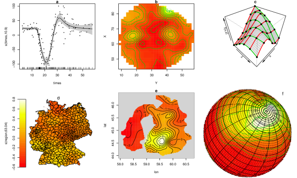
Figure 1: Some of the rich variety of smooths available in the mgcv package. From top right: A simple one dimensional adaptive smooth; multidimensional thin-plate splines; multidimensional tensor product smooths; Gaussian Markov random fields; soap film finite area smoothers; splines on the sphere.

In principle, the JAGS package and language allows Bayesian inference about a very wide range of models that can be written as directed acyclic graphs (DAG). This class includes GAMs as one special case. The Bayesian view of spline smoothing and additive models is almost as old as splines and additive models themselves (kimeldorfwahba1970; wahba83; silverman85; hastie2000bayesBF; fahrmeir.lang), and several authors have exploited this to use JAGS or BUGS (bugs) for generalized additive modelling, notably crainiceanu2005 based on ruppert.wand.carroll and zuurGAMM.

In principle the mgcv package already included all the code required to set up smoothers for use with JAGS. This is because what is required is essentially the same as what is required to use any standard mixed modelling software for GAM inference: for example mgcv function gamm based on the appendix of wood04 uses the nlme package (nlme) in this way. However, a considerable degree of user expertise is required to implement this reliably in practice.

A particular area where difficulty can arise is in the use of centring constraints on model smooth components. Usually additive smooth model structures only make statistical sense if such constraints are applied (see e.g., h&t90), otherwise there is a global intercept associated with each smooth. However the JAGS requirement for all priors to be proper, means that failing to implement such constraints will not cause complete failure of Gibbs sampling. Instead one may see very wide credible intervals and poor mixing, but not realise that this is a model formulation problem rather than a statistical inevitability.

2 The jagam function

The new mgcv function jagam is designed to be called in the same way that the modelling function gam would be called. That is, a model formula and family object specify the required model structure, while the required data are supplied in a data frame or list or on the search path. However, unlike gam, jagam does no model fitting. Rather it writes JAGS code to specify the model as a Bayesian graphical model for simulation with JAGS, and produces a list containing the data objects referred to in the JAGS code, suitable for passing to JAGS via the rjags (rjags) function jags.model.

A simple model, with two univariate smooths and one tensor product smooth, exemplifies the approach. Suppose that we have a data frame, dat, containing the response and predictor variables, have loaded the mgcv package and have used setwd to set the working directory to something appropriate. The code R> jd <- jagam(y   s(x0) + te(x1, x2) + s(x3), data = dat, R+ family = Gamma(link=log), file = "test.jags") would specify a simple log gamma additive model structure,

$$\log(\mu_{i})=f_{1}(x_{0i})+f_{2}(x_{1i},x_{2i})+f_{3}(x_{3i}),~{}~{}~{}~{}y_{i}\sim\Gamma(\mu_{i},\phi),$$

where $f_{2}$ is a scale invariant tensor product smoother, appropriate for representing smooth interaction terms. jagam returns a list containing standard mgcv GAM setup information (pregam) and a list, jags.data, containing the objects required by JAGS for model simulation. The function also writes a JAGS model specification in the file test.jags, as follows. model eta <- X for (i in 1:n) mu[i] <- exp(eta[i]) ## expected response for (i in 1:n) y[i]   dgamma(r,r/mu[i]) ## response r   dgamma(.05,.005) ## scale parameter prior scale <- 1/r ## convert r to standard GLM scale ## Parameteric effect priors CHECK tau is appropriate! for (i in 1:1) b[i]   dnorm(0,0.001) ## prior for s(x0)… K1 <- S1[1:9,1:9] * lambda[1] + S1[1:9,10:18] * lambda[2] b[2:10]   dmnorm(zero[2:10],K1) ## prior for te(x1,x2)… K2 <- S2[1:24,1:24] * lambda[3] + S2[1:24,25:48] * lambda[4] + S2[1:24,49:72] * lambda[5] b[11:34]   dmnorm(zero[11:34],K2) ## prior for s(x3)… K3 <- S3[1:9,1:9] * lambda[6] + S3[1:9,10:18] * lambda[7] b[35:43]   dmnorm(zero[35:43],K3) ## smoothing parameter priors CHECK… for (i in 1:7) lambda[i]   dgamma(.05,.005) rho[i] <- log(lambda[i]) The comments are auto-generated and designed to make it easy to locate the model components, and to draw attention to parts that the user might wish to modify.

In normal use the file would be edited to include the more complex stochastic components likely to have been the motivation for taking a Gibbs sampling approach. It can of course be used un-modified to simply simulate from the posterior of the model parameters, as in the following example code. R> require(rjags) R> jm <- jags.model("test.jags", data = jd$jags.data,R+inits=jd$jags.ini, n.adapt = 2000, n.chains = 1) R> sam <- jags.samples(jm, c("b", "rho", "scale"), n.iter = 10000, R+ thin = 10) The chains should then be checked for convergence and reasonable mixing in the standard ways. R package coda facilitates this (coda).

If all is in order, then many users would want to use the simulation output directly, but the utility function sim2gam can also be used to convert the simulation output into a reduced version of a fitted gam object, suitable for further use with standard mgcv functions. For example R> jam <- sim2jam(sam, jd$pregam)R>par(mfrow=c(1,3));plot(jam)yieldsFigure\text{<span class="ltx\_ref ltx\_missing\_label ltx\_font\_italic ltx\_ref\_self">LABEL:gamma-eg</span>}.\text{Figure 2Figure 22Figure 22PlotsofproglangJAGSestimatedsmoothcomponentsofaloggammaadd}$