On Super-Planckian thermal emission in far field regime

Abstract

We study, in the framework of the Landauer theory, the thermal emission in far-field regime, of arbitrary indefinite planar media and finite size systems. We prove that the flux radiated by the former is bounded by the blackbody emission while, for the second, there is in principle, no upper limit demonstrating so the possibility for a super-Planckian thermal emission with finite size systems.

Since the pioneer works of Kirchoff Kirchoff and Planck Planck on the thermal emission radiated by a hot body, the blackbody was considered as the perfect thermal emitter. Hence, it was admitted so far that no system could radiate more energy into the far-field than a blackbody at the same temperature. However, during the last decade, several studies Nefedov ; Simovski ; Sergeant have claimed that some metamaterials can radiate energy beyond the blackbody limit allowing so a super-Planckian thermal emission. In this brief communication we investigate this problem using the Landauer formalism recently introduced to deal with radiative heat exchanges between 2  PBA2010 ; Biehs2010 or N objects PBAEtAl2011 ; Messina ; Riccardo ; Riccardo2 both in near and far-field regimes. We first consider the problem of the upper bound for far-field thermal emission for arbitrary indefinite planar systems before focusing our attention on finite size systems.

To start, let us consider two arbitrary semi-infinite planar anisotropic media separated by a distance $d\gg\lambda_{\rm th}$ as sketched in Fig. 1. $\lambda_{\rm th}$ is the thermal wavelength given by Wien’s law. According to the fluctuational electrodynamics theory RytovBook1989 the radiative heat flux exchanged between these two media results from the thermal motion of microscopic charges within both materials which are held at a fixed temperature $T_{1}$ and $T_{2}$. The microscopic fluctuating charges lead to macroscopic fluctuating currents $\mathbf{J}^{\rm e}$ in each body which are the sources of fluctuating fields which can be formally written down as

$$\mathbf{E}(\mathbf{r},\omega)={\rm i}\omega\mu_{0}\int_{V}\!\!\mathds{G}^{\rm EE}(\mathbf{r},\mathbf{r}^{\prime},\omega)\cdot\mathbf{J}^{\rm e}(\mathbf{r}^{\prime\prime}\omega),$$ (1)

$$\mathbf{H}(\mathbf{r},\omega)={\rm i}\omega\mu_{0}\int_{V}\!\!\mathds{G}^{\rm HE}(\mathbf{r},\mathbf{r}^{\prime},\omega)\cdot\mathbf{J}^{\rm e}(\mathbf{r}^{\prime\prime}\omega),$$ (2)

where the integration is performed over the volume $V$ containing the source currents $\mathbf{J}^{\rm e}$; $\mu_{0}$ is the permeability of vacuum. The Greens functions $\mathds{G}^{\rm EE}$ and $\mathds{G}^{\rm HE}$ which establish the linear relations between the fields and the sources of the fields are connected by Faraday’s law

$$\mathds{G}^{\rm HE}(\mathbf{r},\mathbf{r}^{\prime},\omega)=\frac{1}{{\rm i}\omega\mu_{0}}\nabla\times\mathds{G}^{\rm EE}(\mathbf{r},\mathbf{r}^{\prime},\omega).$$ (3)

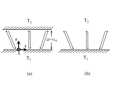
Figure 1: Sketch of (a) two interacting arbitrary planar systems and (b) a planar system in interaction with a thermal bath.

With the above expressions it is straight forward to determine the correlation functions of the fluctuating fields generated by the source currents. For our purpose we are interested in the correlation function $\langle E_{\alpha}(\mathbf{r},t)H_{\beta}(\mathbf{r}^{\prime},t^{\prime})\rangle$ for $\alpha,\beta=x,y,z$ which are statistical averages of the fields with respect to ensembles of the fluctuating currents. Therefore it is necessary to know the statistical properties of the source currents which are given according to the fluctuation-dissipation theorem by Callen

$$\langle J_{\alpha}^{\rm e}(\omega)J_{\beta}^{\rm e}(\omega^{\prime})\rangle=4\pi\omega\Theta(T)\epsilon_{0}\epsilon_{\alpha\beta}^{\prime\prime}\delta(\mathbf{r-r^{\prime}})\delta(\omega+\omega^{\prime}),$$ (4)

where $\epsilon_{0}$ is the permittivity of vacuum and $\uuline{\epsilon}^{\prime\prime}$ is the imaginary part of the permittivity tensor $\uuline{\epsilon}$ of the medium containing the source currents. The applicability of the fluctuation-dissipation theorem requires that the media are at a local thermal equilibrium at temperature $T=T_{1}/T_{2}$. As a shorthand notation we have further introduced the mean energy of a harmonic oscillator at thermal equilibrium

$$\Theta(T)=\frac{\hbar\omega}{2}+\frac{\hbar\omega}{e^{\hbar\omega\beta}-1},$$ (5)

which has in general contributions from vacuum and thermal fluctuations. Here $\beta=1/(k_{\rm B}T)$ is the inverse temperature and $k_{\rm B}$ is Boltzmann’s constant. The part of the vacuum fluctuations can be neglected in the final expression since it does not contribute to the heat flux RytovBook1989 . It follows that the correlation functions of field outside the media containing the source currents are

$$\begin{split}\langle&E_{\alpha}(\mathbf{r},t)H_{\beta}(\mathbf{r}^{\prime},t^{\prime})\rangle=\int_{-\infty}^{+\infty}\!\!\frac{d\omega}{2\pi}e^{i\omega(t-t^{\prime})}2\frac{\omega^{3}}{c^{2}}\mu_{0}\Theta(T)\\ &\quad\times\!\!\int_{V}\!\!d^{3}r^{\prime\prime}\,\mathds{G}^{\rm EE}(\mathbf{r},\mathbf{r}^{\prime\prime},\omega)\cdot\uuline{\epsilon}^{\prime\prime}(\mathbf{r}^{\prime\prime})\cdot{\mathds{G}^{\rm HE}}^{\dagger}(\mathbf{r}^{\prime},\mathbf{r}^{\prime\prime},\omega),\end{split}$$ (6)

where $c$ is the vacuum light velocity. We emphasize that this expression is general and is valid for any anisotropic non-magnetic material with an arbitrary shape which is held at a fixed temperature $T$. Its generalization to magnetic materials is of course straight forward. From this expression we can determine the mean Poynting vector $\langle S_{\alpha}(\mathbf{r},t)\rangle=\eta_{\alpha\beta\gamma}\langle E_{\beta}(\mathbf{r},t)H_{\gamma}(\mathbf{r},t)\rangle$ which determines the amount of energy per unit time and unit area emitted by a medium at a given temperature. Here $\eta_{\alpha\beta\gamma}$ denotes the total antisymetric Levi-Civita tensor.

In order to determine the heat radiated by a medium it is necessary to evaluate expression (6) which can be done if the Green’s function $\mathds{G}^{\rm EE}(\mathbf{r},\mathbf{r}^{\prime\prime})$ is known. As for the magnetic Green’s function, it can then be calculated with Eq. (3). That means we need the Green’s function with the source points $\mathbf{r}^{\prime\prime}$ inside the medium and the observation points $\mathbf{r}$ outside the medium. This procedure can be quite cumbersome in particular if the medium is anisotropic. In such cases it is useful to convert the volume integral into a surface integral. Using Green’s theorem we obtain

$$\begin{split}\int_{V}\!\!d^{3}\mathbf{r}^{\prime}\mathds{G}^{\rm EE}(\mathbf{r},\mathbf{r}^{\prime\prime},\omega)&\cdot\uuline{\epsilon}^{\prime\prime}(\mathbf{r}^{\prime\prime})\cdot{\mathds{G}^{\rm HE}}^{\dagger}(\mathbf{r}^{\prime},\mathbf{r}^{\prime\prime},\omega)\\ &=-\frac{1}{2{\rm i}k_{0}^{2}}\mathds{I}^{\rm S}-\frac{1}{k_{0}^{2}}{\rm Im}\left(\mathds{G}^{\rm HE}(\mathbf{r,r})\right)\end{split}$$ (7)

with the surface integral tensor

$$\begin{split}\mathds{I}^{\rm S}&:=\int_{\partial V}{\rm d}S^{\prime}\biggl{[}\bigl{(}\nabla^{\prime}\times{\mathds{G}^{\rm EE}}^{t}(\mathbf{r},\mathbf{r}^{\prime})\bigr{)}^{t}\cdot\bigl{(}\mathbf{n}\times{\mathds{G}^{\rm HE}}^{\dagger}(\mathbf{r,r^{\prime}})\bigr{)}\\ &\qquad+\mathds{G}^{\rm EE}(\mathbf{r},\mathbf{r}^{\prime})\cdot\bigl{(}\mathbf{n}\times\nabla^{\prime}\times{\mathds{G}^{\rm HE}}^{\dagger}(\mathbf{r,r^{\prime}})\bigr{)}\biggr{]}.\end{split}$$ (8)

Here $\mathbf{n}$ is the surface normal on the boundary $\partial V$ of volume $V$; $t$ and $\dagger$ symbolize the transposition and the hermitian conjugation of the Greens tensors and $k_{0}=\omega/c$ is the wave vector in vacuum. By means of this expression we can use Eq. (6) to write the mean Poynting vector as

$$\begin{split}\langle S_{\gamma}(\mathbf{r},t)&\rangle=\eta_{\alpha\beta\gamma}\langle E_{\alpha}(\mathbf{r},t)H_{\beta}(\mathbf{r},t)\rangle\\ &=\eta_{\alpha\beta\gamma}\int_{0}^{\infty}\!\!\frac{{\rm d}\omega}{2\pi}2\frac{\omega^{3}}{c^{2}}\mu_{0}\Theta(T)\frac{{\rm i}}{2k_{0}^{2}}\mathds{I}^{\rm S}_{\alpha\beta}+\text{c.c.}\end{split}$$ (9)

The advantage of this expression is obviously that it is only necessary to know the Greens function $\mathds{G}^{\rm EE}(\mathbf{r,r^{\prime}})$ with observation and source points outside the material. That means in particular that we do not need to determine the fields inside the medium itself. Furthermore we have replaced a volume integral by a surface integral which makes the calculation simpler. Note that the same expression was found by Narayanaswamy and Zheng Naraya .

In a planar geometry with a translational symmetry in x- and y-direction the Green tensor can be decomposed in plane waves. The resulting Weyl expression has the form

$$\mathds{G}^{\rm EE}(\mathbf{r,r^{\prime}})=\int\!\!\frac{d^{2}\kappa}{(2\pi)^{2}}\mathds{G}^{\rm EE}(\mathbf{\kappa},z)e^{i\boldsymbol{\kappa}\cdot(\mathbf{x-x^{\prime}})}.$$ (10)

The integral is a two-dimensional integral in $k_{x}$-$k_{y}$ space; $\boldsymbol{\kappa}:=(k_{x},k_{y})^{t}$ and $\mathbf{x}=(x,y)^{t}$. For $z^{\prime}<z$ the integrand $\mathds{G}^{\rm EE}(\mathbf{\kappa},z)$ can be written as Opt_Exp

$$\begin{split}\mathds{G}^{\rm EE}(\mathbf{\kappa},z)&=\frac{{\rm i}}{2k_{z}}\bigl{[}\mathds{D}_{12}\bigl{(}e^{{\rm i}k_{z}(z-z^{\prime})}\mathds{1}_{+}+e^{{\rm i}k_{z}(z+z^{\prime})}\mathds{R}_{1}\bigr{)}\\ &\quad+\mathds{D}_{21}\bigl{(}\mathds{R}_{2}\mathds{R}_{1}e^{-{\rm i}k_{z}(z-z^{\prime})}e^{2{\rm i}k_{z}d}\\ &\quad+\mathds{R}_{2}e^{-{\rm i}k_{z}(z+z^{\prime})}e^{2{\rm i}k_{z}d}\bigr{)}]\end{split}$$ (11)

where $k_{z}=\sqrt{k_{0}^{2}-\kappa^{2}}$ is the normal component of the wave vector. Here we have introduced the unit and reflection operators in polarization basis ($i,j={\rm s},{\rm p}$)

$$\mathds{1}_{\pm} :=\sum_{i}\mathbf{a}_{i}^{\pm}\otimes\mathbf{a}_{i}^{\pm},$$ (12)

$$\mathds{R}_{1} :=\sum_{i,j}r_{ij}^{(1)}\mathbf{a}_{i}^{+}\otimes\mathbf{a}_{j}^{-},$$ (13)

$$\mathds{R}_{2} :=\sum_{i,j}r_{ij}^{(2)}\mathbf{a}_{i}^{-}\otimes\mathbf{a}_{j}^{+}.$$ (14)

The polarization vectors for s- and p-polarization are defined as

$$\mathbf{a}_{\rm s}^{\pm}:=\frac{1}{\kappa}\begin{pmatrix}k_{y}\\ -k_{x}\\ 0\end{pmatrix}$$ (15)

and

$$\mathbf{a}_{\rm p}^{\pm}:=\frac{1}{\kappa k_{0}}\begin{pmatrix}\mp k_{x}k_{z}\\ \mp k_{y}k_{z}\\ \kappa^{2}\end{pmatrix}.$$ (16)

The reflection coefficients $r_{ij}^{(1/2)}$ are the Fresnel reflection coefficients of interface $1$ and $2$ describing how an incoming $j$-polarized wave is reflected into a $i$-polarized wave, while $\mathds{D}_{ij}$ is the multiple scattering operator defined as

$$\mathds{D}_{12} :=(\mathds{1}_{+}-\mathds{R}_{1}\mathds{R}_{2}e^{2{\rm i}k_{z}d})^{-1},$$ (17)

$$\mathds{D}_{21} :=(\mathds{1}_{-}-\mathds{R}_{2}\mathds{R}_{1}e^{2{\rm i}k_{z}d})^{-1}.$$ (18)

It follows according to (9) and (10) that the net flux $\Phi=\langle S_{z}\rangle$ (power per unit surface) exchanged between two arbitrary anisotropic media Opt_Exp separated by a distance $d$ larger than the thermal wavelength $\lambda_{\rm th}$ can be written into a Landauer-like form

$$\Phi=2\int_{0}^{\infty}\frac{{\rm d}\omega}{2\pi}\,[\Theta(T_{1})-\Theta(T_{2})]\underset{\mid\boldsymbol{\kappa}\mid<\omega/c}{\int}\frac{{\rm d}^{2}\boldsymbol{\kappa}}{(2\pi)^{2}}\mathcal{T}(\omega,\boldsymbol{\kappa},d),$$ (19)

where we have defined the transmission coefficient $\mathcal{T}$ as

$$\mathcal{T}(\omega,\boldsymbol{\kappa},d):=\frac{1}{2}{\rm Tr}\bigl{[}(\mathds{1}_{+}-\mathds{R}_{2}^{\dagger}\mathds{R}_{2})\mathds{D}_{12}(\mathds{1}_{+}-\mathds{R}_{1}\mathds{R}_{1}^{\dagger}){\mathds{D}_{12}}^{\dagger}\bigr{]}.$$ (20)

Note that this expression is in accordance with results found by several other groups with different methods Bimonte ; Messina2011 ; Krueger2012 . When the second medium is a bosonic field, then $\mathds{R}_{2}=\mathds{O}$ (no reflecting medium) so that the transmission coefficient simplifies to

$$\mathcal{T}(\omega,\boldsymbol{\kappa},d)=\frac{1}{2}{\rm Tr}\bigl{[}\mathds{1}_{+}-\mathds{R}_{1}\mathds{R}^{\dagger}_{1}]=1-\frac{1}{2}\parallel\mathds{R}_{1}\parallel_{F}^{2},$$ (21)

where

$$\parallel\mathds{R}_{1}\parallel_{F}^{2}=\mid r^{ss}\mid^{2}+\mid r^{pp}\mid^{2}+\mid r^{sp}\mid^{2}+\mid r^{ps}\mid^{2}$$ (22)

is the squared Frobenius norm of reflection operator. Since $2\geq\parallel\mathds{R}_{1}\parallel_{F}^{2}\geq 0$, the net flux exchanged between the medium and its surrounding is bounded by the maximal flux

$$\Phi_{\rm max}=2\int_{0}^{\infty}\frac{{\rm d}\omega}{2\pi}\,[\Theta(T_{1})-\Theta(T_{2})]\underset{\mid\boldsymbol{\kappa}\mid<\omega/c}{\int}\frac{{\rm d}^{2}\boldsymbol{\kappa}}{(2\pi)^{2}}.$$ (23)

Since the $\kappa$-integral gives $\pi k_{0}^{2}$ (circle with radius $k_{0}$)

$$\begin{split}\Phi_{\rm max}&=\frac{c}{4}\int_{0}^{\infty}\!\!{\rm d}\omega\bigl{[}\Theta(T_{1})-\Theta(T_{2})\bigr{]}\frac{\omega^{2}}{\pi^{2}c^{3}}\\ &=\int_{0}^{\infty}\!\!{\rm d}\omega\bigl{[}I^{0}_{\omega}(T_{1})-I^{0}_{\omega}(T_{2})\bigr{]}\\ &=\sigma(T^{4}_{1}-T^{4}_{2})\end{split}$$ (24)

where

$$\sigma:=\frac{\pi^{2}k_{\rm B}^{4}}{60c^{2}\hbar^{3}}=5.670373\cdot 10^{-8}\>\rm W.\rm m^{-2}.\rm K^{-4}$$ (25)

is Stefan-Boltzmann’s constant and

$$I^{0}_{\omega}(T):=\Theta(T)\frac{\omega^{2}}{4\pi^{2}c^{2}}$$ (26)

is the spectral intensity of a black body. The such derived upper bound (24) unambiguously proves that the power radiated by any planar isotropic or anisotropic material into its surrounding is always smaller or equal to the power that would be radiated by a blackbody at the same temperature. It is important to note that this limit exist not only for the total flux where the upper bound is set by the Stefan-Boltzmann’s law but also spectrally where the upper bound is set by $I^{0}_{\omega}(T_{1})-I^{0}_{\omega}(T_{2})$.

The same limit applies of course also for the more general situation of radiative heat transfers between two planar media. This is simply the case, because there can only be a maximal transmission into medium 2 if all the incoming propagating waves are perfectly transmitted into medium 2. This is achieved if the reflectivity of medium 2 is zero, i.e. $\mathds{R}_{2}=\mathds{0}$. This is exactly the condition which lead to Stefan-Boltzmann’s law. Therefore the blackbody law provides the upper limit for heat radiation between planar materials even if they are anisotropic.

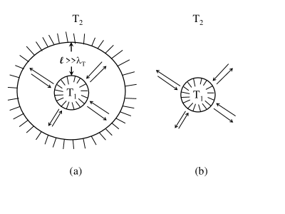
Figure 2: Sketch of (a) a finite size medium in interaction with an encompassing system and (b) a finite size system in interaction with a thermal bath.

Now, let us consider the case of finite size systems. A natural generalization of the previous configuration is the case of a sphere of radius $R$ encompassed by another sphere as illustrated in Fig. 2. As previously, the two bodies are hold at two different temperatures and separated by a shell of thickness $l\gg\lambda_{\rm th}$. By following the same course of action as in the plane-plane configuration, the net power exchanged between these media can be expressed in a Landauer-like form

$$Q=\int_{0}^{\infty}\frac{{\rm d}\omega}{2\pi}\,[\Theta(T_{1})-\Theta(T_{2})]\mathcal{T}(\omega),$$ (27)

where the transmission coefficient $\mathcal{T}(\omega)$ can be expressed in terms of the surface integral tensor in Eq. (8) (see Ref. Naraya ). Using $I^{0}$ from Eq. (26), the blackbody intensity at the frequency $\omega$, the net power exchanged between both media becomes

$$Q=\int_{0}^{\infty}{\rm d}\omega 2\pi\frac{c^{2}}{\omega^{2}}[I^{0}_{\omega}(T_{1})-I^{0}_{\omega}(T_{2})]\mathcal{T}(\omega).$$ (28)

Since $Q$ is the difference of the thermal emissions of the sphere and the wall it can also be written in terms of the thermal emissivity emissivity $\epsilon(\omega)$ which we introduce in the usual manner such that

$$Q=A\int_{0}^{\infty}{\rm d}\omega\epsilon(\omega)[I^{0}_{\omega}(T_{1})-I^{0}_{\omega}(T_{2})],$$ (29)

where $A=4\pi R^{2}$ is the surface area of the spherical body. Hence, if the emissivity would be constant $\epsilon(\omega)\equiv\epsilon$, then we would obtain the well-known expression

$$Q=A\epsilon\sigma(T_{1}^{4}-T_{2}^{4})$$ (30)

for the exchanged power. The comparison of relations (28) and (29) shows that the relation between the emissivity and the transmission coefficient is

$$\epsilon(\omega)=\frac{1}{2R^{2}}\frac{c^{2}}{\omega^{2}}\mathcal{T}(\omega).$$ (31)

Of course, the emissivity is related to the absorptivity inside the spherical body Bohren — as demanded by Kirchhoff’s law — and the absorptivity itself can be written in terms of the absorption cross-section $\sigma_{a}(\omega)$. It follows that Bohren

$$\epsilon(\omega)=\frac{\sigma_{a}(\omega)}{\pi R^{2}}.$$ (32)

Therefore, we have also a relation between the transmission coefficient and the absorption cross-section

$$\mathcal{T}(\omega)=\frac{2}{\pi}\frac{\omega^{2}}{c^{2}}\sigma_{a}(\omega).$$ (33)

In arbitrary core-shell geometric configuration, the absorption cross-section reads Qiu

$$\begin{split}\sigma_{a}(\omega)&=\frac{\pi}{2}\frac{c^{2}}{\omega^{2}}\sum_{p={\rm TE,TM}}\sum_{l=1}^{\infty}(2l+1)(1-\mid r_{p,l}\mid^{2}),\end{split}$$ (34)

where the summation is done over all channels (spherical waves) of TE and TM polarization, $r_{p,l}$ being the reflection coefficient of the system for the $l^{th}$ spherical order. It follows from relation (33) that the transmission coefficient takes the simple form

$$\mathcal{T}(\omega)=\sum_{p={\rm TE,TM}}\sum_{l=1}^{\infty}(2l+1)(1-\mid r_{p,l}\mid^{2}).$$ (35)

Contrary to the plane-plane configuration, a direct inspection of this serie shows that there is, in principle, no intrinsic upper limit for the flux $\Phi=\frac{Q}{A}$ (power per unit surface) exchanged between both media, where $A$ is the surface area of the inner sphere with radius $R$. Indeed, provided the medium can support higher order modes Fan1 ; Fan2 ; JP_PBA these modes will increase the transmission coefficient such that the emissivity can become larger than one. Such behavior has been predicted long time ago with strong dissipating sphere in Eisner , for instance, and has also been discussed in several textbooks as in the famous Bohren and Huffman’s book Bohren . Therefore Eq. (30) is not necessarily an upper limit in this case. And indeed, very recent works have found that core-shell particles MaslovskiEtAl2016 and cylinders GolykEtAl2012 can show a super-Planckian emission which is not a contradiction to the blackbody law, because it simply does not apply for finite size objects Bohren .

In conclusion, we have shown that thermal radiation of a planar anisotropic medium is limited by Stefan-Boltzmann’s law, so that planar media cannot show Super-Planckian far-field emission. On the other hand, for finite size media Stefan-Boltzmann’s does not apply. As an example we discussed this for a spherical particle. In this case expression (35) for the transmission coefficient provides a natural target to be optimized within the Planck window in order to realize a finite size super-Planckian emitter. This optimization consists in minimizing the reflection coefficients for a maximum number of spherical channels and therefore to maximize the absorption cross-section of system. This is a direct consequence of reciprocity principle for the light as explicited by the generalized Kirchoff law RytovBook1989 .

References

(1) G. Kirchhoff, Monatsberichte der Akademie der Wissenschaften zu Berlin, sessions of Dec., 783 (1859).
(2) M. Planck, Ann. Phys. 309, 553 (1901).
(3) I.S. Nefedov, L. A. Melnikov, Appl.Phys.Lett. 105, 1610902 (2014).
(4) C. Simovski,S. Maslovski, I. Nefedov, Igor; S. Kosulnikov , P. Belov, S.Tretyakov, Photonics and Nanostructures-Fundamentals and applications, 13, 31, (2015).
(5) Z. Yu, N.P. Sergeant, T. Skauli, G. Zhang, H. Wang, S.Fan, Nature Communications 4 1730 (2013).
(6) P. Ben-Abdallah and K. Joulain, Phys. Rev. B 82, 121419(R) (2010).
(7) S.-A. Biehs, E. Rousseau, and J.-J. Greffet, Phys. Rev. Lett. 105, 234301 (2010).
(8) P. Ben-Abdallah, S.-A. Biehs, and K. Joulain, Phys. Rev. Lett. 107, 114301 (2011).
(9) R. Messina, M. Antezza and P. Ben-Abdallah, Phys. Rev. Lett. 109, 244302 (2012).
(10) R. Messina, M. Tschikin, S.-A. Biehs, and P. Ben-Abdallah, Phys. Rev. B 88, 104307 (2013).
(11) R. Messina and M. Antezza, Phys. Rev. A 89, 052104 (2014).
(12) S. M. Rytov, Y. A. Kravtsov, and V. I. Tatarskii, Principles of Statistical Radiophysics 3 (Springer-Verlag, 1989).
(13) H. B. Callen and T. A. Welton, Phys. Rev. 83, 34 (1951).
(14) S.A. Biehs, P. Ben-Abdallah, F. S. S. Rosa, K. Joulain, J. J. Greffet, Optics Express, 19 , A1088-A1103 (2011).
(15) G. Bimonte and E. Santamato, Phys. Rev. A 76, 013810 (2007).
(16) R. Messina and M. Antezza, Phys. Rev. A 84, 042102 (2011).
(17) M. Krüger, G. Bimonte, T. Emig, and M. Kardar, Phys. Rev. B 86, 115423 (2012).
(18) A. I. Volokitin and B. N. J. Persson, Rev. Mod. Phys. 79, 1291(2007).
(19) A. Narayanaswamy and Y. Zheng, J. Quant. Spect. Rad. Transf. 132,12 , (2014).
(20) Y. Zheng and A. Ghanekar J. Appl. Phys. 117, 064314 (2015).
(21) W. Qiu, B. G. DeLacy, S. G. Johnson, J. D. Joannopoulos and M. Soljacic, Optics Express, 20 , 18494-18504 (2012).
(22) Z. Ruan and S. Fan, Phys. Rev. Lett. 105, 013901 (2010).
(23) Z. Ruan and S. Fan, Appl. Phys. Lett. 98, 043101 (2011).
(24) J.P. Hugonin, M. Besbes and P. Ben-Abdallah, Phys. Rev. B(R) 91, 18, 180202 ( 2015).
(25) G. W. Kattawar and M. Eisner, Appl. Opt. 9, 12 (1970).
(26) C. F. Bohren and D. R. Huffman, Absorption and Scattering of Light by Small Paricles (Wiley, New York ,1998).
(27) Stanislav I. Maslovski, Constantin R. Simovski, Sergei A. Tretyakov, New J. Phys. 18 013034 (2016).
(28) V. A. Golyk, M. Krüger, and M. Kardar, Phys. Rev. E 85, 046603 (2012).