Corrected Discrete Approximations for the
Conditional and Unconditional Distributions of the
Continuous Scan Statistic

Abstract

The (conditional or unconditional) distribution of the continuous scan statistic in a one-dimensional Poisson process may be approximated by that of a discrete analogue via time discretization (to be referred to as the discrete approximation). With the help of a change-of-measure argument, we derive the first-order term of the discrete approximation which involves some functionals of the Poisson process. Richardson’s extrapolation is then applied to yield a corrected (second-order) approximation. Numerical results are presented to compare various approximations.

Keywords: Poisson process; Richardson’s extrapolation; Markov chain embedding; change of measure; second-order approximation; stochastic geometry.

1 Introduction

The subject of scan statistics in one dimension as well as in higher dimensions has found a great many applications in diverse areas ranging from astronomy to epidemiology, genetics and neuroscience. See Glaz, Naus and Wallenstein [11] and Glaz and Naus [9] for a thorough review and comprehensive discussion of scan distribution theory, methods and applications. See also Glaz, Pozdnyakov and Wallenstein [10] for a collection of articles on recent developments.

In the one-dimensional setting, let $\Pi$ be a (homogeneous) Poisson point process of intensity $\lambda>0$ on the (normalized) unit interval $(0,1]$. For a specified window size $0<w<1$ and integers $N\geq k\geq 2$, we are interested in finding the conditional and unconditional probabilities

$$P(k;N,w):=\mathbb{P}(S_{w}\geq k\mid|\Pi|=N)\;\;\mathrm{and}\;\;P^{\ast}(k;\lambda,w):=\mathbb{P}(S_{w}\geq k),$$

where $|\Pi|$ is the cardinality of the point set $\Pi$ (i.e. the total number of Poisson points) and

$$S_{w}=S_{w}(\Pi):=\max_{0\leq t\leq 1-w}\left|\Pi\cap(t,t+w]\raisebox{11.38109pt}{}\right|,$$

the maximum number of Poisson points within any window of size $w$. The (continuous) scan statistic $S_{w}$ arises from the likelihood ratio test for the null hypothesis $\mathcal{H}_{0}:$ the intensity function $\lambda(t)=\lambda$ (constant) against the alternative $\mathcal{H}_{a}:$ $\lambda(t)=\lambda+\Delta\mathbf{1}_{(a,a+w]}(t)$ for (unknown) $0\leq a\leq 1-w$ and $\Delta>0$ where $\mathbf{1}_{\mathcal{A}}$ denotes the indicator function of a set $\mathcal{A}$.

By applying results on coincidence probabilities and the generalized ballot problem (cf. Karlin and McGregor [17] and Barton and Mallows [1]), Huntington and Naus [12] and Hwang [15] derived closed-form expressions for $P(k;N,w)$ which require to sum a large number of determinants of large matrices and hence are in general not amenable to numerical evaluation. Later by exploiting the fact that $P(k;N,w)$ is piecewise polynomial in $w$ with (finitely many) different polynomials of $w$ in different ranges, Neff and Naus [21] developed a more computationally feasible approach and presented extensive tables for the exact $P(k;N,w)$ for various combinations of $(k,N,w)$ with $N\leq 25$. (More precisely, each number in the tables has an error bounded by $10^{-9}$.) Noting that $P^{\ast}(k;\lambda,w)$ is a weighted average of $P(k;N,w)$ over $N$ (with Poisson probabilities as weights), they also provided tables for $P^{\ast}(k;\lambda,w)$ with $\lambda\leq 16$ where the error size for each tabulated number varies depending on the combination of $(k,\lambda,w)$. (The errors tend to be greater for smaller values of $w$.) Huffer and Lin [13, 14] developed an alternative approach (based on spacings) to computing the exact $P(k;N,w)$.

Instead of finding the exact $P^{\ast}(k;\lambda,w)$, Naus [20] proposed an accurate product-type approximation based on a heuristic (approximate) Markov property while Janson [16] derived some sharp bounds. See also Glaz and Naus [8] for related results in a discrete setting. Treating the problem as boundary crossing for a two-dimensional random field, Loader [19] obtained effective large deviation approximations for the tail probability of the scan statistic in one and higher dimensions. For more general large deviation approximation results, see Siegmund and Yakir [22], Chan and Zhang [2] and Fang and Siegmund [4].

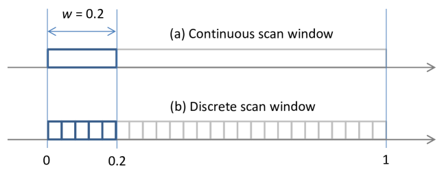
Figure 1: The continuous and discrete scan windows

The continuous scan statistic $S_{w}$ may be approximated by a discrete analogue via time discretization. Specifically, assuming $w=p/q$ ($p,q$ relatively prime integers), partition the (time) interval $(0,1]$ into $n$ subintervals of length $n^{-1}$, $n$ a multiple of $q$ (cf. Figure 1 with $w=1/5,n=25$). Each subinterval (independently) contains either no point (with probability $1-\lambda/n$) or exactly one point (with probability $\lambda/n$). Since a window of size $w$ covers $nw$ subintervals, as an approximation to $S_{w}$, we define the discrete scan statistic $S_{w}^{(n)}$ to be the maximum number of points within any $nw$ consecutive subintervals. For large $n$, $P^{\ast}(k;\lambda,w)=\mathbb{P}(S_{w}\geq k)$ may be approximated by $\mathbb{P}(S_{w}^{(n)}\geq k)$, which can be readily calculated using the Markov chain embedding method (cf. [5, 6, 18]). Indeed, it is known that $\mathbb{P}(S_{w}\geq k)-\mathbb{P}(S_{w}^{(n)}\geq k)=O(n^{-1})$ (cf. [7, 23]).

In Section 2, as $n$ (multiple of $q$) tends to infinity, we derive the limit of $n[\mathbb{P}(S_{w}\geq k)-\mathbb{P}(S_{w}^{(n)}\geq k)]$, which involves some functionals of $\Pi$. In order to establish this limit result, we find it instructive to introduce a slightly different discrete scan statistic (denoted $S^{\prime(n)}_{w}$) which is stochastically smaller than $S_{w}$ and $S_{w}^{(n)}$. With a coupling device, we derive the limits of $n[\mathbb{P}(S_{w}\geq k)-\mathbb{P}(S^{\prime(n)}_{w}\geq k)]$ and $n[\mathbb{P}(S_{w}^{(n)}\geq k)-\mathbb{P}(S^{\prime(n)}_{w}\geq k)]$. In Section 3, using a change-of-measure argument, a similar result is obtained for the conditional probability $\mathbb{P}(S_{w}\geq k\mid|\Pi|=N)$. Based on these limit results, Richardson’s extrapolation is then applied to yield second-order approximations for the conditional and unconditional distributions of the continuous scan statistic. In Section 4, numerical results comparing the various approximations are presented along with some discussion.

2 The unconditional case

Recall the window size $w=p/q$ with $p$ and $q$ relatively prime integers. For $n=mq\;(m=1,2,\dots)$, let $H^{n}_{i},i=1,\dots,n$, be $i.i.d.$ with $\mathbb{P}(H^{n}_{i}=0)=1-\lambda/n$ and $\mathbb{P}(H^{n}_{i}=1)=\lambda/n$, and let $I^{n}_{i},i=1,\dots,n$, be $i.i.d.$ with $\mathbb{P}(I^{n}_{i}=0)=e^{-\lambda/n}$ and $\mathbb{P}(I^{n}_{i}=1)=1-e^{-\lambda/n}$. The $i.i.d.$ Bernoulli sequence $(H^{n}_{1},\dots,H^{n}_{n})$ approximates the Poisson point process $\Pi$ by matching the expected number of points in each subinterval, i.e.

$$\mathbb{E}(H^{n}_{i})=\mathbb{E}\Big{(}\Big{|}\Pi\cap\Big{(}\frac{i-1}{n},\frac{i}{n}\Big{]}\Big{|}\Big{)}=\frac{\lambda}{n}.$$

On the other hand, the $i.i.d.$ Bernoulli sequence $(I^{n}_{1},\dots,I^{n}_{n})$ approximates $\Pi$ by matching the probability of no point in each subinterval, i.e.

$$\mathbb{P}(I^{n}_{i}=0)=\mathbb{P}\Big{(}\Big{|}\Pi\cap\Big{(}\frac{i-1}{n},\frac{i}{n}\Big{]}\Big{|}=0\Big{)}=e^{-\lambda/n}.$$

The two discrete scan statistics $S^{(n)}_{w}$ and $S^{\prime(n)}_{w}$ are now defined in terms of the two Bernoulli sequences as follows:

$$S^{(n)}_{w} =S^{(n)}_{w,H}:=\max_{i=1\dots,n-nw+1}\sum_{r=i}^{i+nw-1}H^{n}_{r}\;,$$

$$S^{\prime(n)}_{w} =S^{(n)}_{w,I}:=\max_{i=1\dots,n-nw+1}\sum_{r=i}^{i+nw-1}I^{n}_{r}\;.$$

Since $I^{n}_{i}$ is stochastically smaller than $H^{n}_{i}$ and $|\Pi\cap((i-1)/n,i/n]|$, it follows that $S^{(n)}_{w,I}$ is stochastically smaller than $S_{w}$ and $S^{(n)}_{w,H}$. In Sections 2.1 and 2.2, we derive $\lim_{n\to\infty}n[\mathbb{P}(S_{w}\geq k)-\mathbb{P}(S^{(n)}_{w,I}\geq k)]$ and $\lim_{n\to\infty}n[\mathbb{P}(S_{w}\geq k)-\mathbb{P}(S^{(n)}_{w,H}\geq k)]$, respectively.

2.1 Matching the probability of no point

Since the Bernoulli sequence $(I^{n}_{1},\dots,I^{n}_{n})$ and $\Pi$ match in the probability of no point in each subinterval, it is instructive to define $(I^{n}_{1},\dots,I^{n}_{n})$ in terms of $\Pi$ as follows:

$$I_{i}^{n}=\mathbf{1}\Big{\{}\Pi\cap\Big{(}\frac{i-1}{n},\frac{i}{n}\Big{]}\neq\emptyset\Big{\}},\;i=1,\dots,n.$$

Thus, $(I^{n}_{1},\dots,I^{n}_{n})$ and $\Pi$ are defined on the same probability space. In particular, $S_{w}\geq S_{w,I}^{(n)}$ with probability $1$. For fixed $w=p/q$ and for each (fixed) $k=2,3,\dots$, let

$$\alpha =\mathbb{P}(\mathcal{A}),\;\;\mbox{where}\;\;\mathcal{A}=\mathcal{A}_{k,w}:=\{S_{w}\geq k\},$$

$$\alpha_{n} =\mathbb{P}(\mathcal{A}_{n}),\;\;\mbox{where}\;\;\mathcal{A}_{n}=\mathcal{A}_{n,k,w}:=\{S^{(n)}_{w,I}\geq k\}.$$

Note that $\alpha=P^{\ast}(k;\lambda,w)$ defined in Section 1. In order to derive the limit of $n(\alpha-\alpha_{n})$ as $n\to\infty$, we need to introduce some functionals of $\Pi$. Let $M:=|\Pi|$, which is a Poisson random variable with mean $\lambda$. Writing $\Pi=\{Q_{1},\dots,Q_{M}\}$, assume (with probability $1$) that $0<Q_{1}<\cdots<Q_{M}<1$. Further assume (with probability $1$) that $w\notin\Pi,1-w\notin\Pi$, and $Q_{j}\pm w\notin\Pi$ for $j=1,\dots,M$ (i.e. $Q_{j}-Q_{i}\neq w$ for all $1\leq i<j\leq M$). Define the functionals $\nu(\Pi)=\nu(\{Q_{1},\dots,Q_{M}\})$ and $\tilde{\nu}(\Pi)=\tilde{\nu}(\{Q_{1},\dots,Q_{M}\})$ as follows:

$$\nu(\Pi):= \sum_{\{\ell:Q_{\ell}<1-w\}}\mathbf{1}\left\{\raisebox{14.22636pt}{}\right.S_{w}<k,\left|\Pi\cap(Q_{\ell},Q_{\ell}+w]\raisebox{11.38109pt}{}\right|=k-2,$$

$$\mbox{~{}~{}~{}~{}~{}~{}~{}~{}~{}~{}~{}~{}~{}~{}~{} $\left|\Pi\cap(t,t+w]\raisebox{11.38109pt}{}\right|\leq k-2$ for all $t$ with $Q_{\ell}\leq t\leq Q_{\ell}+w$}\left.\raisebox{14.22636pt}{}\right\},$$

$$\tilde{\nu}(\Pi):= \sum_{\ell=1}^{M}\mathbf{1}\left\{S_{w}<k,\;\max_{0\leq t\leq 1-w}\left|(\Pi\cup\{Q_{\ell}\})\cap(t,t+w]\raisebox{11.38109pt}{}\right|=k\right\},$$

where $\Pi\cup\{Q_{\ell}\}$ is interpreted as a multiset with $Q_{\ell}$ having multiplicity $2$.

Theorem 2.1.

For $n=mq\;(m=1,2,\dots)$,

$$\lim_{n\to\infty}n(\alpha-\alpha_{n})~{}=~{}\frac{\lambda}{2}~{}\mathbb{E}\left[\nu(\Pi)+\tilde{\nu}(\Pi)\raisebox{11.38109pt}{}\right].$$

Proof.

Denoting the complement of $\mathcal{A}_{n}$ by $\mathcal{A}_{n}^{c}$ and noting that $\mathcal{A}_{n}\subset\mathcal{A}$, we have $\alpha-\alpha_{n}=\mathbb{P}(\mathcal{A})-\mathbb{P}(\mathcal{A}_{n})=\mathbb{P}(\mathcal{A}\cap\mathcal{A}_{n}^{c})$. For $i=1,\dots,n$, let

$$\tilde{I}^{n}_{i}=\Big{|}\Pi\cap\Big{(}\frac{i-1}{n},\frac{i}{n}\Big{]}\Big{|},\;\mbox{the number of Poisson points in the $i$-th subinterval}.$$

Then $\tilde{I}^{n}_{i}=0$ implies $I_{i}^{n}=0$ and $\tilde{I}_{i}^{n}\geq 1$ implies $I_{i}^{n}=1$. Consider the following disjoint events

$$\hskip 31.29802pt\mathcal{G}_{1}\hskip 5.12149pt = \{\tilde{I}_{j}^{n}\leq 1,j=1,\dots,n\},$$

$$\hskip 31.29802pt\mathcal{G}_{2,i} = \{\tilde{I}_{i}^{n}=2,\tilde{I}_{j}^{n}\leq 1\mbox{ for all $j\neq i$}\},~{}i=1,\dots,n,$$

$$\hskip 31.29802pt\mathcal{G}_{3}\hskip 5.12149pt = \{\tilde{I}_{j}^{n}=\tilde{I}_{j^{\prime}}^{n}=2\mbox{ for some $j\neq j^{\prime}$}\}\cup\{\tilde{I}_{j}^{n}\geq 3\mbox{ for some $j$}\}.$$

We have

$$\hskip 31.29802pt\alpha-\alpha_{n} ~{}= \mathbb{P}(\mathcal{A}\cap\mathcal{A}_{n}^{c})\hskip 216.24094pt$$

$$~{}= \mathbb{P}(\mathcal{A}\cap\mathcal{A}_{n}^{c}\cap\mathcal{G}_{1})+\sum_{i=1}^{n}\mathbb{P}(\mathcal{A}\cap\mathcal{A}_{n}^{c}\cap\mathcal{G}_{2,i})+\mathbb{P}(\mathcal{A}\cap\mathcal{A}_{n}^{c}\cap\mathcal{G}_{3}).$$ (1)

Claim that

$$\hskip 31.29802pt\mathbb{P}(\mathcal{A}\cap\mathcal{A}_{n}^{c}\cap\mathcal{G}_{1})\hskip 5.12149pt = \frac{1}{2}\sum_{i=1}^{n-nw}P_{i}^{(n)}+~{}O(n^{-2}),$$ (2)

$$\hskip 31.29802pt\sum_{i=1}^{n}\mathbb{P}(\mathcal{A}\cap\mathcal{A}_{n}^{c}\cap\mathcal{G}_{2,i}) = \sum_{i=1}^{n}\widetilde{P}_{i}^{(n)}+~{}O(n^{-2}),$$ (3)

$$\hskip 31.29802pt\mathbb{P}(\mathcal{A}\cap\mathcal{A}_{n}^{c}\cap\mathcal{G}_{3})\hskip 5.12149pt = O(n^{-2}),$$ (4)

where

$$P_{i}^{(n)}=\mathbb{P}\left(\mathcal{A}_{n}^{c},\sum_{r=i+1}^{i+nw-1}I_{r}^{n}=k-2,I_{i}^{n}=I_{i+nw}^{n}=1\right),~{}i=1,\dots,n-nw,$$ (5)

$$\widetilde{P}_{i}^{(n)}=\mathbb{P}\left(\mathcal{A}_{n}^{c},\tilde{I}_{i}^{n}=2,\sum_{r=i^{\prime}}^{i^{\prime}+nw-1}I_{r}^{n}=k-1\mbox{ for some $i^{\prime}$ with}\right.\hskip 45.5244pt$$ (6)

$$\hskip 39.83385pt\left.1\leq i^{\prime}\leq i\leq i^{\prime}+nw-1\leq n\raisebox{17.07164pt}{}\right),~{}i=1,\dots,n.$$

Since $\mathbb{P}(\mathcal{G}_{3})=O(n^{-2})$, (4) follows easily. To prove (2), note that when $\tilde{I}_{i}^{n}\leq 1$ for all $i$ (i.e. on the event $\mathcal{G}_{1}$), each subinterval $((i-1)/n,i/n]$ contains at most one Poisson point. If $\tilde{I}_{i}^{n}=1$, denote the only Poisson point in $((i-1)/n,i/n]$ by $Q_{(i)}$ whose location is uniformly distributed over $((i-1)/n,i/n]$. When $\tilde{I}_{i}^{n}\leq 1$ for all $i$, in order for $\mathcal{A}\cap\mathcal{A}_{n}^{c}$ to occur, there must exist some pair $(i,i^{\prime})$ with $i^{\prime}=i+nw$ such that

$$\sum_{r=i+1}^{i^{\prime}-1}\tilde{I}_{r}^{n}=k-2,\;\tilde{I}_{i}^{n}=\tilde{I}_{i^{\prime}}^{n}=1,\;\mbox{and }Q_{(i^{\prime})}-Q_{(i)}<w.$$

So we have $\mathcal{A}\cap\mathcal{A}_{n}^{c}\cap\mathcal{G}_{1}=\cup_{i=1}^{n-nw}\mathcal{G}_{1,i}$ where for $i=1,\dots,n-nw$,

$$\begin{array}[]{r}\mathcal{G}_{1,i}=\mathcal{A}_{n}^{c}\cap\left\{\tilde{I}_{j}^{n}\leq 1\mbox{ for all $j$, }\displaystyle\sum_{r=i+1}^{i+nw-1}\tilde{I}_{r}^{n}=k-2,\right.\\ \left.\displaystyle\tilde{I}_{i}^{n}=\tilde{I}_{i+nw}^{n}=1,\;\mbox{and }Q_{(i+nw)}-Q_{(i)}<w\raisebox{14.22636pt}{}\right\}.\end{array}$$

Since

$$\sum_{1\leq i<j\leq n-nw}\mathbb{P}(\tilde{I}_{i}^{n}=\tilde{I}_{i+nw}^{n}=\tilde{I}_{j}^{n}=\tilde{I}_{j+nw}^{n}=1)=O(n^{-2}),$$

we have

$$\mathbb{P}(\mathcal{A}\cap\mathcal{A}_{n}^{c}\cap\mathcal{G}_{1}) = \sum_{i=1}^{n-nw}\mathbb{P}(\mathcal{G}_{1,i})+O(n^{-2})$$ (7)

$$= \frac{1}{2}\sum_{i=1}^{n-nw}\mathbb{P}(\mathcal{G}_{1,i}^{\prime})+O(n^{-2}),$$

where

$$\mathcal{G}_{1,i}^{\prime}=\mathcal{A}_{n}^{c}\cap\left\{\tilde{I}_{j}^{n}\leq 1\mbox{ for all $j$, }\displaystyle\sum_{r=i+1}^{i+nw-1}\tilde{I}_{r}^{n}=k-2,\;\tilde{I}_{i}^{n}=\tilde{I}_{i+nw}^{n}=1\right\}.$$

In (7), we have used the facts that $\tilde{I}_{1}^{n},\dots,\tilde{I}_{n}^{n}$ are independent and that given $\tilde{I}_{i}^{n}=\tilde{I}_{i+nw}^{n}=1$, $Q_{(i)}$ and $Q_{(i+nw)}$ are (conditionally) independent and uniformly distributed over $((i-1)/n,i/n]$ and $((i+nw-1)/n,(i+nw)/n]$, respectively, so that $Q_{(i+nw)}-Q_{(i)}<w$ with (conditional) probability 1/2, which implies $\mathbb{P}(\mathcal{G}_{1,i})=\frac{1}{2}\mathbb{P}(\mathcal{G}_{1,i}^{\prime})$. For $i=1,\dots,n-nw$, define

$$\mathcal{G}_{1,i}^{\prime\prime}=\mathcal{A}_{n}^{c}\cap\left\{\sum_{r=i+1}^{i+nw-1}I_{r}^{n}=k-2,\;I_{i}^{n}=I_{i+nw}^{n}=1\right\},$$ (8)

which is the event inside the parentheses on the right-hand side of (5), so that $P_{i}^{(n)}=\mathbb{P}(\mathcal{G}_{1,i}^{\prime\prime})$. Note that $\mathcal{G}_{1,i}^{\prime}\subset\mathcal{G}_{1,i}^{\prime\prime}$ and that $\mathcal{G}_{1,i}^{\prime\prime}\setminus\mathcal{G}_{1,i}^{\prime}$ is contained in

$$\{I_{i}^{n}=I_{i+nw}^{n}=1,\;\tilde{I}_{j}^{n}\geq 2\mbox{ for some $j$}\},$$

which has a probability of order $n^{-3}$. By (7),

$$\mathbb{P}(\mathcal{A}\cap\mathcal{A}_{n}^{c}\cap\mathcal{G}_{1})=\frac{1}{2}\sum_{i=1}^{n-nw}\mathbb{P}(\mathcal{G}_{1,i}^{\prime\prime})+O(n^{-2})=\frac{1}{2}\sum_{i=1}^{n-nw}P_{i}^{(n)}+O(n^{-2}),$$

establishing (2).

To prove (3), let $\mathcal{H}=\{I_{j}=I_{j+nw}=1\mbox{ for some $1\leq j\leq n-nw$}\}$. On $\mathcal{G}_{2,i}\cap\mathcal{H}^{c}$, in order for $\mathcal{A}\cap\mathcal{A}_{n}^{c}$ to occur, there must exist some $i^{\prime}$ with $1\leq i^{\prime}\leq i\leq i^{\prime}+nw-1\leq n$ such that $\sum_{r=i^{\prime}}^{i^{\prime}+nw-1}I_{r}^{n}=k-1$ (implying that $\sum_{r=i^{\prime}}^{i^{\prime}+nw-1}\tilde{I}_{r}^{n}=k$). It follows that $\mathcal{A}\cap\mathcal{A}_{n}^{c}\cap\mathcal{G}_{2,i}\cap\mathcal{H}^{c}\subset\mathcal{G}_{2,i}^{\prime}\subset\mathcal{A}\cap\mathcal{A}_{n}^{c}\cap\mathcal{G}_{2,i}$, where

$$\mathcal{G}_{2,i}^{\prime}=\mathcal{A}_{n}^{c}\cap\left\{\raisebox{14.22636pt}{}\tilde{I}_{i}^{n}=2,\;\tilde{I}_{j}^{n}\leq 1\mbox{ for all $j\neq i$},\right.\hskip 142.26378pt$$

$$\hskip 28.45274pt\left.\sum_{r=i^{\prime}}^{i^{\prime}+nw-1}I^{n}_{r}=k-1\mbox{ for some $i^{\prime}$ with }1\leq i^{\prime}\leq i\leq i^{\prime}+nw-1\leq n\right\}.$$

Since $\mathbb{P}(\mathcal{G}_{2,i}\cap\mathcal{H})=O(n^{-3})$, we have $\sum_{i=1}^{n}\mathbb{P}(\mathcal{G}_{2,i}\cap\mathcal{H})=O(n^{-2})$, implying that

$$\sum_{i=1}^{n}\mathbb{P}(\mathcal{A}\cap\mathcal{A}_{n}^{c}\cap\mathcal{G}_{2,i})=\sum_{i=1}^{n}\mathbb{P}(\mathcal{G}_{2,i}^{\prime})+O(n^{-2})=\sum_{i=1}^{n}\mathbb{P}(\mathcal{G}_{2,i}^{\prime\prime})+O(n^{-2}),$$

where

$$\mathcal{G}_{2,i}^{\prime\prime}=\mathcal{A}_{n}^{c}\cap\left\{\tilde{I}_{i}^{n}=2,\sum_{r=i^{\prime}}^{i^{\prime}+nw-1}I_{r}^{n}=k-1\right.\hskip 113.81102pt$$

$$\hskip 28.45274pt\left.\mbox{ for some $i^{\prime}$ with $1\leq i^{\prime}\leq i\leq i^{\prime}+nw-1\leq n$}\raisebox{14.22636pt}{}\right\}.$$

(Note that $\mathcal{G}_{2,i}^{\prime}\subset\mathcal{G}_{2,i}^{\prime\prime}$ and $\mathcal{G}_{2,i}^{\prime\prime}\setminus\mathcal{G}_{2,i}^{\prime}$ is contained in the event $\{\tilde{I}_{i}^{n}=2,\tilde{I}_{j}^{n}\geq 2\mbox{ for some $j\neq i$}\}$, which has a probability of order $n^{-3}$.) By (6), $\widetilde{P}_{i}^{(n)}=\mathbb{P}(\mathcal{G}_{2,i}^{\prime\prime})$. This establishes (3).

By (1)–(4), we have

$$\alpha-\alpha_{n}=\frac{1}{2}\sum_{i=1}^{n-nw}P_{i}^{(n)}+\sum_{i=1}^{n}\widetilde{P}_{i}^{(n)}+O(n^{-2}).$$ (9)

For $i=1,\dots,n-nw$, let $P_{i}^{\prime(n)}=\mathbb{P}(\mathcal{F}_{i})$ where

$$\mathcal{F}_{i} :=\mathcal{A}_{n}^{c}\cap\Big{\{}\sum_{r=i+1}^{i+nw-1}I_{r}^{n}=k-2,I^{n}_{i}=1,I^{n}_{i+nw}=0,\;\mbox{sum of any $nw$}$$

$$\mbox{~{}~{}~{}~{}~{}~{}~{}~{}~{}~{}~{}~{} consecutive $I^{n}_{r}$ including $r=i+nw$ is at most $k-2$}\Big{\}}.$$

Claim that

$$P_{i}^{(n)}/P_{i}^{\prime(n)}=\rho_{n}\mbox{~{}~{}for all~{}~{}}i=1,\dots,n-nw,$$ (10)

where

$$\rho_{n}:=\frac{\mathbb{P}(I_{i+nw}^{n}=1)}{~{}\mathbb{P}(I_{i+nw}^{n}=0)~{}}~{}=~{}\frac{~{}1-e^{-\lambda/n}~{}}{e^{-\lambda/n}}~{}=~{}e^{\lambda/n}-1.$$

To establish the claim, recall that $P_{i}^{(n)}=\mathbb{P}(\mathcal{G}_{1,i}^{\prime\prime})$ where $\mathcal{G}_{1,i}^{\prime\prime}$ (cf. (8)) depends only on $(I^{n}_{1},\dots,I^{n}_{n})$. It is instructive to interpret $\mathcal{G}_{1,i}^{\prime\prime}$ as a collection of configurations $(I^{n}_{1},\dots,I^{n}_{n})=(h_{1},\dots,h_{n})$ where $(h_{1},\dots,h_{n})$ satisfies $h_{j}=0$ or $1$ for all $j$, $h_{i}=h_{i+nw}=1$, and

$$\max_{j=1,\dots,n-nw+1}\sum_{r=j}^{j+nw-1}h_{r}<k\;,\;\;\sum_{r=i+1}^{i+nw-1}h_{r}=k-2.$$

Likewise, the event $\mathcal{F}_{i}$ is a collection of configurations $(I^{n}_{1},\dots,I^{n}_{n})=(h^{\prime}_{1},\dots,h^{\prime}_{n})$ where $(h^{\prime}_{1},\dots,h^{\prime}_{n})$ satisfies $h^{\prime}_{j}=0$ or $1$ for all $j$, $h^{\prime}_{i}=1,h^{\prime}_{i+nw}=0$,

$$\max_{j=1,\dots,n-nw+1}\sum_{r=j}^{j+nw-1}h^{\prime}_{r}<k\;,\;\;\sum_{r=i+1}^{i+nw-1}h^{\prime}_{r}=k-2,$$

and sum of any $nw$ consecutive $h^{\prime}_{r}$ including $r=i+nw$ is at most $k-2$. It is readily seen that a configuration $(I^{n}_{1},\dots,I^{n}_{n})=(h_{1},\dots,h_{n})$ is in $\mathcal{G}_{1,i}^{\prime\prime}$ if and only if the configuration $(I^{n}_{1},\dots,I^{n}_{n})=(h^{\prime}_{1},\dots,h^{\prime}_{n})$ is in $\mathcal{F}_{i}$ where $(h^{\prime}_{1},\dots,h^{\prime}_{n})=(h_{1},\dots,h_{n})-\mathbf{e}_{i+nw}$ with $\mathbf{e}_{i+nw}$ being the vector of zeroes except for the $(i+nw)$-th entry being $1$. The claim (10) now follows from the independence property of $I^{n}_{1},\dots,I^{n}_{n}$.

By (10),

$$\rho^{-1}_{n}\sum_{i=1}^{n-nw}P_{i}^{(n)}=\sum_{i=1}^{n-nw}P_{i}^{\prime(n)} =\sum_{i=1}^{n-nw}\mathbb{P}(\mathcal{F}_{i})=\mathbb{E}\left[{\nu}^{(n)}(\Pi)\right],$$ (11)

where

$${\nu}^{(n)}(\Pi):= \sum_{i=1}^{n-nw}\mathbf{1}\left\{\mathcal{A}_{n}^{c},\sum_{r=i+1}^{i+nw-1}I_{r}^{n}=k-2,I^{n}_{i}=1,I^{n}_{i+nw}=0,\mbox{ sum of any}\right.$$

$$\left.\mbox{~{}~{}~{}~{}~{}~{}~{}~{}$nw$ consecutive $I^{n}_{r}$ including $r=i+nw$ is at most $k-2$}\raisebox{14.22636pt}{}\right\}.$$

To deal with $\widetilde{P}^{(n)}_{i},i=1,\dots,n$, let

$$\widetilde{P}^{\prime(n)}_{i}:=\mathbb{P}\left(\mathcal{A}_{n}^{c},I_{i}^{n}=1,\sum_{r=i^{\prime}}^{i^{\prime}+nw-1}I_{r}^{n}=k-1\;\mbox{ for some $i^{\prime}$ with}\right.\hskip 28.45274pt$$

$$\left.1\leq i^{\prime}\leq i\leq i^{\prime}+nw-1\leq n\raisebox{14.22636pt}{}\right).$$

By an argument similar to the proof of (10), we have $\widetilde{P}_{i}^{(n)}/\widetilde{P}_{i}^{\prime(n)}=\tilde{\rho}_{n}$ for all $i=1,\dots,n$ where

$$\tilde{\rho}_{n}~{}=~{}\frac{\mathbb{P}(\tilde{I}_{i}^{n}=2)}{~{}\mathbb{P}(I_{i}^{n}=1)~{}}~{}=~{}\frac{e^{-\lambda/n}(\lambda/n)^{2}}{~{}2(1-e^{-\lambda/n})~{}}.$$

So,

$$\tilde{\rho}_{n}^{-1}\sum_{i=1}^{n}\widetilde{P}_{i}^{(n)}~{}=~{}\sum_{i=1}^{n}\widetilde{P}_{i}^{\prime(n)}=\mathbb{E}\left[\tilde{\nu}^{(n)}(\Pi)\right],$$ (12)

where

$$\tilde{\nu}^{(n)}(\Pi):=\sum_{i=1}^{n}\mathbf{1}\left\{\mathcal{A}_{n}^{c},I_{i}^{n}=1,\sum_{r=i^{\prime}}^{i^{\prime}+nw-1}I_{r}^{n}=k-1\right.\hskip 79.66771pt$$

$$\hskip 28.45274pt\left.\mbox{ for some $i^{\prime}$ with }1\leq i^{\prime}\leq i\leq i^{\prime}+nw-1\leq n\raisebox{17.07164pt}{}\right\}.$$

Since $\rho_{n}=\lambda/n+O(n^{-2})$ and $\tilde{\rho}_{n}=\lambda/(2n)+O(n^{-2})$, it follows from (9), (11) and (12) that

$$n(\alpha-\alpha_{n})-\frac{\lambda}{2}\;\mathbb{E}\left[\nu^{(n)}(\Pi)+\tilde{\nu}^{(n)}(\Pi)\right]=O(n^{-1}).$$ (13)

Note that $\nu^{(n)}(\Pi)$ and $\tilde{\nu}^{(n)}(\Pi)$ converge a.s. to $\nu(\Pi)$ and $\tilde{\nu}(\Pi)$, respectively. Since

$$\max\{\nu^{(n)}(\Pi),\tilde{\nu}^{(n)}(\Pi)\}~{}\leq~{}\sum_{i=1}^{n}\mathbf{1}\{I^{n}_{i}=1\}~{}\leq~{}\left|\Pi\right|,$$

we have by the dominated convergence theorem that $\mathbb{E}[\nu^{(n)}(\Pi)+\tilde{\nu}^{(n)}(\Pi)]$ converges to $\mathbb{E}[\nu(\Pi)+\tilde{\nu}(\Pi)]$, which together with (13) completes the proof. ∎

Remark 2.1.

With a little more effort, it can be shown that

$$\mathbb{E}\left[\nu^{(n)}(\Pi)+\tilde{\nu}^{(n)}(\Pi)\right]-\mathbb{E}\left[\nu(\Pi)+\tilde{\nu}(\Pi)\raisebox{11.38109pt}{}\right]=O(n^{-1}),$$

which together (13) yields

$$\alpha-\alpha_{n}=C_{\alpha}n^{-1}+O(n^{-2}),$$ (14)

where

$$C_{\alpha}=\frac{\lambda}{2}\mathbb{E}\left[\nu(\Pi)+\tilde{\nu}(\Pi)\raisebox{11.38109pt}{}\right].$$ (15)

2.2 Matching the expected number of points

Recall that $H_{i}^{n},i=1,\dots,n$ are i.i.d. with $\mathbb{P}(H_{i}^{n}=0)=1-\lambda/n$ and $\mathbb{P}(H_{i}^{n}=1)=\lambda/n$. Let $\beta_{n}=\mathbb{P}(\mathcal{B}_{n})$ where

$$\mathcal{B}_{n}=\mathcal{B}_{n,k,w}:=\{S^{(n)}_{w,H}\geq k\}=\left\{\max_{i=1,\dots,n-nw+1}\sum_{r=i}^{i+nw-1}H_{r}^{n}~{}\geq~{}k\right\}.$$

Lemma 2.1.

For $n=mq\;(m=1,2,\dots)$,

$$\lim_{n\to\infty}\frac{2n}{\lambda^{2}}(\beta_{n}-\alpha_{n})=-\alpha+\int_{0}^{1}\mathbb{P}\left(\max_{0\leq t\leq 1-w}\left|(\Pi\cup\{u\})\cap(t,t+w]\raisebox{14.22636pt}{}\right|\geq k\right)du.$$

Proof.

Let $L_{i}^{n},i=1,\dots,n$ be i.i.d. and independent of $I_{1}^{n},\dots,I_{n}^{n}$ such that $\mathbb{P}(L_{i}^{n}=0)=(1-\lambda/n)e^{\lambda/n}=1-\mathbb{P}(L_{i}^{n}=1)$. Letting $\tilde{L}_{i}^{n}=\max\{I_{i}^{n},L_{i}^{n}\}$ and noting that $\mathbb{P}(\tilde{L}_{i}^{n}=0)=\mathbb{P}(I_{i}^{n}=0\mbox{ and }L_{i}^{n}=0)=1-\lambda/n=\mathbb{P}(H_{i}^{n}=0)$, we have $\mathcal{L}(\tilde{L}_{1}^{n},\dots,\tilde{L}_{n}^{n})=\mathcal{L}(H_{1}^{n},\dots,H_{n}^{n})$ where $\mathcal{L}(\mathbf{V})$ denotes the law of a random vector $\mathbf{V}$, so that $\beta_{n}=\mathbb{P}(\mathcal{B}_{n})=\mathbb{P}(\widetilde{\mathcal{B}}_{n})$ where

$$\widetilde{\mathcal{B}}_{n}=\left\{\max_{i=1,\dots,n-nw+1}\sum_{r=i}^{i+nw-1}\tilde{L}_{r}^{n}~{}\geq~{}k\right\}.$$

Since $I_{i}^{n}=1$ implies $\tilde{L}_{i}^{n}=1$, we have $\mathcal{A}_{n}\subset\widetilde{\mathcal{B}}_{n}$. Letting $S_{n}=\sum_{i=1}^{n}L_{i}^{n}$ and noting that $\widetilde{\mathcal{B}}_{n}\cap\{S_{n}=0\}=\mathcal{A}_{n}\cap\{S_{n}=0\}$ and that

$$\mathbb{P}(S_{n}=0)=1-\frac{\lambda^{2}}{2n}+O(n^{-2}),~{}\mathbb{P}(S_{n}=1)=\frac{\lambda^{2}}{2n}+O(n^{-2}),~{}\mathbb{P}(S_{n}\geq 2)=O(n^{-2}),$$

we have

$$\beta_{n}=\mathbb{P}(\widetilde{\mathcal{B}}_{n})= ~{}\mathbb{P}(\widetilde{\mathcal{B}}_{n}|S_{n}=0)\mathbb{P}(S_{n}=0)+\mathbb{P}(\widetilde{\mathcal{B}}_{n}|S_{n}=1)\mathbb{P}(S_{n}=1)$$

$$~{}+\mathbb{P}(\widetilde{\mathcal{B}}_{n}|S_{n}\geq 2)\mathbb{P}(S_{n}\geq 2)$$

$$= ~{}\mathbb{P}(\mathcal{A}_{n}|S_{n}=0)\left(1-\frac{\lambda^{2}}{2n}\right)+\mathbb{P}(\widetilde{\mathcal{B}}_{n}|S_{n}=1)\frac{\lambda^{2}}{2n}+O(n^{-2})$$

$$= ~{}\alpha_{n}\left(1-\frac{\lambda^{2}}{2n}\right)+\mathbb{P}(\widetilde{\mathcal{B}}_{n}|S_{n}=1)\frac{\lambda^{2}}{2n}+O(n^{-2}).$$ (16)

Claim that

$$\lim_{n\to\infty}\mathbb{P}(\widetilde{\mathcal{B}}_{n}|S_{n}=1)=\displaystyle\int_{0}^{1}\mathbb{P}\left(\max_{0\leq t\leq 1-w}\Big{|}(\Pi\cup\{u\})\cap(t,t+w]\Big{|}\geq k\right)du,$$ (17)

which together with (16) yields the desired result.

It remains to establish the claim (17). Let $Q$ be a random point which is uniformly distributed on $(0,1]$ and independent of $\Pi$. Let

$$\hat{I}^{n}_{i}=\mathbf{1}\Big{\{}(\Pi\cup\{Q\})\cap\Big{(}\frac{i-1}{n},\frac{i}{n}\Big{]}\neq\emptyset\Big{\}},\;\;i=1,\dots,n.$$

It is readily seen that $\mathcal{L}(\tilde{L}^{n}_{1},\dots,\tilde{L}^{n}_{n}\mid S_{n}=1)=\mathcal{L}(\hat{I}^{n}_{1},\dots,\hat{I}^{n}_{n})$, which implies $\mathbb{P}(\widetilde{\mathcal{B}}_{n}|S_{n}=1)=\mathbb{P}(\hat{\mathcal{B}}_{n}),$ where

$$\hat{\mathcal{B}}_{n}=\left\{\max_{i=1,\dots,n-nw+1}\sum_{r=i}^{i+nw-1}\hat{I}_{r}^{n}~{}\geq~{}k\right\}.$$

Since $\mathbf{1}_{\hat{\mathcal{B}}_{n}}$ converges a.s. to $\mathbf{1}\{\max_{0\leq t\leq 1-w}|(\Pi\cup\{Q\})\cap(t,t+w]|\geq k\}$, we have

$$\lim_{n\to\infty}\mathbb{P}(\hat{\mathcal{B}}_{n}) =\mathbb{P}\Big{(}\max_{0\leq t\leq 1-w}\Big{|}(\Pi\cup\{Q\})\cap(t,t+w]\Big{|}\geq k\Big{)}$$

$$=\displaystyle\int_{0}^{1}\mathbb{P}\left(\max_{0\leq t\leq 1-w}\Big{|}(\Pi\cup\{u\})\cap(t,t+w]\Big{|}\geq k\right)du,$$

the claim (17) follows. This completes the proof of the lemma. ∎

Theorem 2.2.

$$\lim_{n\to\infty}\frac{2n}{\lambda^{2}}(\alpha-\beta_{n})~{}=~{} \displaystyle\frac{1}{\lambda}\mathbb{E}\left[\nu(\Pi)+\tilde{\nu}(\Pi)\raisebox{11.38109pt}{}\right]+\alpha\vspace*{1mm}$$

$$-\displaystyle\int_{0}^{1}\mathbb{P}\left(\max_{0\leq t\leq 1-w}\left|(\Pi\cup\{u\})\cap(t,t+w]\raisebox{14.22636pt}{}\right|\geq k\right)du.$$

Proof.

Note that

$$\frac{2n}{\lambda^{2}}(\alpha-\beta_{n})=\frac{2n}{\lambda^{2}}(\alpha-\alpha_{n})-\frac{2n}{\lambda^{2}}(\beta_{n}-\alpha_{n}),$$

which together with Theorem 2.1 and Lemma 2.2 yields the desired result. ∎

Remark 2.2.

Similarly to (14), it can be shown that

$$\alpha-\beta_{n}=C_{\beta}n^{-1}+O(n^{-2}),$$ (18)

where

$$C_{\beta} =\frac{1}{2}\lambda^{2}\alpha+\frac{\lambda}{2}\mathbb{E}\left[\nu(\Pi)+\tilde{\nu}(\Pi)\raisebox{11.38109pt}{}\right]$$

$$\;\;\;\;\;-\frac{\lambda^{2}}{2}\int_{0}^{1}\mathbb{P}\left(\max_{0\leq t\leq 1-w}\Big{|}(\Pi\cup\{u\})\cap(t,t+w]\Big{|}\geq k\right)du.$$ (19)

3 The conditional case

Following the notation of Section 2, $\Pi=\{Q_{1},\dots,Q_{M}\}$ is a Poisson point process of intensity $\lambda$ on $(0,1]$, where $M$ is a Poisson random variable with mean $\lambda$. For given $N\geq k=2,3,\dots$, we are interested in approximating

$$\gamma^{(N)}:=P(k;N,w)=\mathbb{P}\left(\left.\max_{0\leq t\leq 1-w}\left|\Pi\cap(t,t+w]\raisebox{11.38109pt}{}\right|\geq k\right|M=N\right).$$

Conditional on $M=N$, the $N$ points $0<Q_{1}<\dots<Q_{N}<1$ are the order statistics of $N$ independent and uniformly distributed random variables on $(0,1]$. Denote by $\Pi^{N}$ a set of $N$ i.i.d. uniform random variables on $(0,1]$. Then $\mathcal{L}(\Pi^{N})=\mathcal{L}(\Pi|M=N)$ and $\gamma^{(N)}=\mathbb{P}(\mathcal{E}^{N})$ where

$$\mathcal{E}^{N}=\mathcal{E}^{N}_{k,w}:=\left\{\max_{0\leq t\leq 1-w}\left|\Pi^{N}\cap(t,t+w]\raisebox{11.38109pt}{}\right|\geq k\right\}.$$

As in Section 2, with $n=mq$ ($m=1,2,\dots$), the interval $(0,1]$ is partitioned into $n$ subintervals of length $n^{-1}$, so that a window of size $w=p/q$ covers $nw$ subintervals. As an approximation to $N$ points uniformly distributed on $(0,1]$, we randomly select $N$ of the $n$ subintervals and assign a point to each of them. Let $J_{i}^{n}=1$ or 0 according to whether or not the $i$-th subinterval is selected (so as to contain a point). Then $\sum_{i=1}^{n}J_{i}^{n}=N$ and for $h_{i}=0$ or 1,

$$\mathbb{P}_{N}(J_{i}^{n}=h_{i},i=1,\dots,n)=\left\{\begin{array}[]{ll}1{\mbox{\LARGE/}}{\mbox{\large${n\choose N}$}},&\hbox{if~{} $\sum_{i=1}^{n}h_{i}=N$,}\\ 0,&\hbox{otherwise,}\end{array}\right.$$

where the subscript $N$ in $\mathbb{P}_{N}$ signifies that there are $N$ 1’s in $J_{1}^{n},\dots,J_{n}^{n}$. While in Section 2, $(I_{1}^{n},\dots,I_{n}^{n})$ is defined in terms of $\Pi$ in order to make use of a coupling argument, there is no natural way to define $(J_{1}^{n},\dots,J_{n}^{n})$ and $\Pi^{N}$ on the same probability space. As no danger of confusion may arise, we will use the same probability measure notation $\mathbb{P}_{N}$ for both the probability space where $\Pi^{N}$ is defined and the probability space where $(J^{n}_{1},\dots,J^{n}_{n})$ is defined. Let

$$\gamma_{n}^{(N)}=\mathbb{P}_{N}(\mathcal{E}_{n}^{N})\;,\;\;\mbox{where}\;\;\mathcal{E}_{n}^{N}:=\left\{\max_{i=1,\dots,n-nw+1}\sum_{r=i}^{i+nw-1}J_{r}^{n}~{}\geq~{}k\right\}.$$ (20)

Theorem 3.3.

For $N$ fixed and $n=mq\;(m=1,2,\dots)$,

$$\lim_{n\to\infty}n(\gamma^{(N)}-\gamma_{n}^{(N)}) = \frac{1}{2}N(N-1)(\gamma^{(N-1)}-\gamma^{(N)})$$

$$\hskip 28.45274pt+~{}\frac{1}{2}N\mathbb{E}\left[\nu(\Pi)+\tilde{\nu}(\Pi)\left|M=N-1\raisebox{11.38109pt}{}\right.\right].$$

Proof.

For notational simplicity, the superscript $N$ in $\mathcal{E}^{N}$ and $\mathcal{E}_{n}^{N}$ is suppressed while to avoid possible confusion, $\mathbb{P}_{N}$ is not abbreviated to $\mathbb{P}$ as later a change-of-measure argument requires consideration of $\mathbb{P}_{N-1}$. Let $\tilde{J}_{i}=\left|\Pi^{N}\cap((i-1)/N,i/N]\raisebox{8.53581pt}{}\right|$, $i=1,\dots,n$, and define the (disjoint) events

$$\begin{array}[]{l}U_{1}=\{\tilde{J}_{j}^{n}\leq 1,j=1,\dots,n\},\vspace*{2mm}\\ U_{2}=\bigcup_{i=1}^{n}U_{2,i},\;U_{2,i}=\{\tilde{J}_{i}^{n}=2,\tilde{J}_{j}^{n}\leq 1\mbox{ for all $j\neq i$}\},\vspace*{2mm}\\ U_{3}=\{\tilde{J}_{j}^{n}=\tilde{J}_{j^{\prime}}^{n}=2\mbox{ for some $j\neq j^{\prime}$}\}\cup\{\tilde{J}_{j}^{n}\geq 3\mbox{ for some $j$}\}.\end{array}$$

We have

$$\mathbb{P}_{N}(U_{1}) = \displaystyle\prod_{i=1}^{N}\left(1-\frac{i-1}{n}\right)~{}=~{}1-\frac{N(N-1)}{2n}+O(n^{-2}),\vspace*{1mm}$$ (21)

$$\mathbb{P}_{N}(U_{2}) = \displaystyle{N\choose 2}n^{-1}\prod_{j=1}^{N-2}\left(1-\frac{j}{n}\right)~{}=~{}\frac{N(N-1)}{2n}+O(n^{-2}),$$ (22)

and $\mathbb{P}_{N}(U_{3})=O(n^{-2})$, so that

$$\gamma^{(N)} = \mathbb{P}_{N}(\mathcal{E}^{N})=\mathbb{P}_{N}(\mathcal{E})\vspace*{2mm}$$ (23)

$$= \mathbb{P}_{N}(\mathcal{E}\cap U_{1})+\mathbb{P}_{N}(\mathcal{E}\cap U_{2})+\mathbb{P}_{N}(\mathcal{E}\cap U_{3})\vspace*{2mm}$$

$$= \mathbb{P}_{N}(\mathcal{E}|U_{1})\mathbb{P}_{N}(U_{1})+\mathbb{P}_{N}(\mathcal{E}\cap U_{2})+O(n^{-2}).$$

We first work on $\mathbb{P}_{N}(\mathcal{E}|U_{1})$. Write $\mathcal{E}=\widetilde{\mathcal{E}}_{n}\cup(\mathcal{E}\cap\widetilde{\mathcal{E}}_{n}^{c})$ where

$$\begin{array}[]{l}\widetilde{\mathcal{E}}_{n}:=\displaystyle\left\{\max_{i=1,\dots,n-nw+1}\sum_{r=i}^{i+nw-1}\tilde{J}_{r}^{n}\geq k\right\}~{}(\subset\mathcal{E}).\end{array}$$

Note that given $U_{1}$, the conditional distribution of $(\tilde{J}_{1}^{n},\dots,\tilde{J}_{n}^{n})$ is equal to the distribution of $(J_{1}^{n},\dots,J_{n}^{n})$ (i.e. $\mathcal{L}(\tilde{J}_{1}^{n},\dots,\tilde{J}_{n}^{n}|U_{1})=\mathcal{L}(J_{1}^{n},\dots,J_{n}^{n}))$, and that $\widetilde{\mathcal{E}}_{n}$ depends on $(\tilde{J}_{1}^{n},\dots,\tilde{J}_{n}^{n})$ in the same way that $\mathcal{E}_{n}=\mathcal{E}^{N}_{n}$ does on $(J_{1}^{n},\dots,J_{n}^{n})$ (cf. (20)). So we have $\mathbb{P}_{N}(\widetilde{\mathcal{E}}_{n}|U_{1})=\mathbb{P}_{N}(\mathcal{E}_{n})=\gamma_{n}^{(N)}$, and

$$\hskip 14.22636pt\mathbb{P}_{N}(\mathcal{E}|U_{1})~{}=~{} \mathbb{P}_{N}(\widetilde{\mathcal{E}}_{n}|U_{1})+\mathbb{P}_{N}(\mathcal{E}\cap\widetilde{\mathcal{E}}_{n}^{c})|U_{1})$$

$$=~{} \gamma_{n}^{(N)}+\mathbb{P}_{N}(\mathcal{E}\cap\widetilde{\mathcal{E}}_{n}^{c}\;|U_{1}).$$ (24)

If $\tilde{J}_{i}^{n}=1$, denote the only point of $\Pi^{N}$ in $((i-1)/n,i/n]$ by $Q_{(i)}$, whose location is uniformly distributed over $((i-1)/n,i/n]$. When $\tilde{J}_{i}^{n}\leq 1$ for all $i$ (i.e. on the event $U_{1}$), in order for

$$\mathcal{E}\cap\widetilde{\mathcal{E}}_{n}^{c}~{}=~{}\left\{\max_{0\leq t\leq 1-w}\left|\Pi^{N}\cap(t,t+w]\raisebox{11.38109pt}{}\right|\geq k\right\}\hskip 85.35826pt\vspace*{1mm}$$

$$\hskip 85.35826pt\cap\left\{\max_{i=0,1,\dots,n-nw}\left|\Pi^{N}\cap\left(\frac{i}{n},\frac{i}{n}+w\right]\raisebox{11.38109pt}{}\right|<k\right\}$$

to occur, there must exist some pair $(i,i^{\prime})$ with $i^{\prime}=i+nw$ such that $\sum_{r=i+1}^{i^{\prime}-1}\tilde{J}_{r}^{n}=k-2$, $\tilde{J}_{i}^{n}=\tilde{J}_{i^{\prime}}^{n}=1$, and $Q_{(i^{\prime})}-Q_{(i)}<w$. So we have

$$\mathcal{E}\cap\widetilde{\mathcal{E}}_{n}^{c}\cap U_{1}=\bigcup_{i=1}^{n-nw}U_{1,i}$$

where for $i=1,\dots,n-nw$,

$$U_{1,i}~{}=~{}\widetilde{\mathcal{E}}_{n}^{c}\cap\left\{\tilde{J}_{j}^{n}\leq 1\mbox{ for all $j$, }\sum_{r=i+1}^{i+nw-1}\tilde{J}_{r}^{n}=k-2,\right.\hskip 28.45274pt\vspace*{1mm}$$

$$\hskip 85.35826pt\left.\tilde{J}_{i}^{n}=\tilde{J}_{i+nw}^{n}=1,\;Q_{(i+nw)}-Q_{(i)}<w\raisebox{17.07164pt}{}\right\}.$$

Since

$$\displaystyle\sum_{1\leq i<j\leq n-nw}\mathbb{P}_{N}(U_{1,i}\cap U_{1,j})\hskip 156.49014pt\vspace*{1mm}$$

$$\leq \displaystyle\sum_{1\leq i<j\leq n-nw}\mathbb{P}_{N}(\tilde{J}_{i}^{n}=\tilde{J}_{i+nw}^{n}=\tilde{J}_{j}^{n}=\tilde{J}_{j+nw}^{n}=1)=O(n^{-2}),$$

we have

$$\mathbb{P}_{N}(\mathcal{E}\cap\widetilde{\mathcal{E}}_{n}^{c}\mid U_{1}) ~{}=~{} \sum_{i=1}^{n-nw}\mathbb{P}_{N}(U_{1,i}|U_{1})+O(n^{-2})$$ (25)

$$~{}=~{} \frac{1}{2}\sum_{i=1}^{n-nw}\mathbb{P}_{N}(U_{1,i}^{\prime}|U_{1})+O(n^{-2}),$$

where for $i=1,\dots,n-nw$,

$$U_{1,i}^{\prime}=\widetilde{\mathcal{E}}_{n}^{c}\cap\left\{\tilde{J}_{j}^{n}\leq 1\mbox{ for all $j$, }\sum_{r=i+1}^{i+nw-1}\tilde{J}_{r}^{n}=k-2,\;\tilde{J}_{i}^{n}=\tilde{J}_{i+nw}^{n}=1\right\}.$$

In (25), we have used the fact that for any given $h_{j}=0$ or 1 ($j=1,\dots,n$) with $\sum_{j=1}^{n}h_{j}=N$ and $h_{i}=h_{i+nw}=1$, conditional on $\tilde{J}_{j}^{n}=h_{j}$, $j=1,\dots,n$, $Q_{(i)}$ and $Q_{(i+nw)}$ are independent and uniformly distributed over $((i-1)/n,i/n]$ and $((i+nw-1)/n,(i+nw)/n]$, respectively, so that $Q_{(i+nw)}-Q_{(i)}<w$ with probability $1/2$, which implies $\mathbb{P}_{N}(U_{1,i}|U_{1})=\frac{1}{2}\mathbb{P}_{N}(U_{1,i}^{\prime}|U_{1})$.

Note that $U_{1,i}^{\prime},i=1,\dots,n$ depend only on $\tilde{J}_{1}^{n},\dots,\tilde{J}_{n}^{n}$. Since $\mathcal{L}(\tilde{J}_{1}^{n},\dots,\tilde{J}_{n}^{n}|$ $U_{1})$ $=\mathcal{L}(J_{1}^{n},\dots,J_{n}^{n})$, we have

$$\mathbb{P}_{N}(U_{1,i}^{\prime}|U_{1})=\mathbb{P}_{N}(V_{i}),\;i=1,\dots,n-nw,$$ (26)

where

$$V_{i}=\mathcal{E}_{n}^{c}\cap\left\{\sum_{r=i+1}^{i+nw-1}J_{r}^{n}=k-2,J_{i}^{n}=J_{i+nw}^{n}=1\right\}.$$

(Note that $V_{i}$ depends on $(J_{1}^{n},\dots,J_{n}^{n})$ in the same way that $U_{1,i}^{\prime}$ does on $(\tilde{J}_{1}^{n},\dots,\tilde{J}_{n}^{n})$.)

We will simplify $\sum_{i=1}^{n-nw}\mathbb{P}_{N}(U_{1,i}^{\prime}|U_{1})=\sum_{i=1}^{n-nw}\mathbb{P}_{N}(V_{i})$ via a change-of measure argument. It is instructive to interpret the event $V_{i}$ as a collection of configurations $(J_{1}^{n},\dots,J_{n}^{n})=(h_{1},\dots,h_{n})$ where $(h_{1},\dots,h_{n})$ satisfies $h_{r}=0$ or $1$ for $r=1,\dots,n$, and

$$\sum_{r=1}^{n}h_{r}=N,\max_{j=1,\dots,n-nw+1}\sum_{r=j}^{j+nw-1}h_{r}<k,~{}\sum_{r=i+1}^{i+nw-1}h_{r}=k-2,~{}h_{i}=h_{i+nw}=1.$$

Let

$$\begin{array}[]{ll}V_{i}^{\ast}=\left\{\displaystyle\sum_{r=1}^{n}J_{r}^{n}=N-1,\max_{j=1,\dots,n-nw+1}\sum_{r=j}^{j+nw-1}J_{r}^{n}<k,\right.\vspace*{1mm}\\ \hskip 42.67912pt\displaystyle\sum_{r=i+1}^{i+nw-1}J_{r}^{n}=k-2,J_{i}^{n}=1,J_{i+nw}^{n}=0,\mbox{ sum of any $nw$}\vspace*{0mm}\\ \hskip 48.36967pt\left.\mbox{consecutive $J_{r}^{n}$ including $r=i+nw$ is at most $k-2$}\raisebox{17.07164pt}{}\right\},\end{array}$$

which is interpreted as a collection of configurations $(J_{1}^{n},\dots,J_{n}^{n})=(h_{1}^{\ast},\dots,h_{n}^{\ast})$, where $(h_{1}^{\ast},\dots,h_{n}^{\ast})$ satisfies $h_{r}^{\ast}=0$ or 1 for $r=1,\dots,n$, and

$$\begin{array}[]{l}\displaystyle\sum_{r=1}^{n}h_{r}^{\ast}=N-1,\max_{j=1,\dots,n-nw+1}\sum_{r=j}^{j+nw-1}h_{r}^{\ast}<k,\sum_{r=i+1}^{i+nw-1}h_{r}^{\ast}=k-2,\vspace*{2mm}\\ \mbox{$h_{i}^{\ast}=1,h_{i+nw}^{\ast}=0$, and sum of any $nw$ consecutive $h_{r}^{\ast}$ including $r$}\vspace*{2mm}\\ \mbox{$=i+nw$ is at most $k-2$.}\end{array}$$

If a configuration $(J_{1}^{n},\dots,J_{n}^{n})=(h_{1},\dots,h_{n})$ is in $V_{i}$, then the configuration $(J_{1}^{n},\dots,J_{n}^{n})=(h_{1}^{\ast},\dots,h_{n}^{\ast})$ is in $V_{i}^{\ast}$ provided $h_{r}^{\ast}=h_{r}$ for all $r\neq i+nw$ and $h_{i+nw}=1$, $h_{i+nw}^{\ast}=0$. In other words, a configuration is in $V_{i}$ if and only if with the $(i+nw)$-th entry replaced by 0, it is in $V_{i}^{\ast}$. Note that the number of nonzero entries for a configuration in $V_{i}^{\ast}$ equals $N-1$. Recall that the notation $\mathbb{P}_{N}$ ($\mathbb{P}_{N-1}$, resp.) denotes the probability measure for $(J_{1}^{n},\dots,J_{n}^{n})$ with $\sum_{r=1}^{n}J_{r}^{n}=N$ ($\sum_{r=1}^{n}J_{r}^{n}=N-1$, resp.). It follows that

$$\frac{\mathbb{P}_{N}(V_{i})}{~{}\mathbb{P}_{N-1}(V_{i}^{\ast})~{}}~{}=~{}\frac{~{}{n\choose N-1}~{}}{{n\choose N}}~{}=~{}\frac{N}{n-N+1}.$$

Therefore,

$$\sum_{i=1}^{n-nw}\mathbb{P}_{N}(V_{i})~{}=~{} \frac{N}{n-N+1}\sum_{i=1}^{n-nw}\mathbb{P}_{N-1}(V_{i}^{\ast})$$

$$=~{} \frac{N}{n-N+1}\mathbb{E}_{N-1}\left[\nu_{1}^{(n)}(J_{1}^{n},\dots,J_{n}^{n})\raisebox{11.38109pt}{}\right],$$ (27)

where

$$\begin{array}[]{l}\nu_{1}^{(n)}(J_{1}^{n},\dots,J_{n}^{n})=\displaystyle\sum_{i=1}^{n-nw}\mathbf{1}\left\{\displaystyle\max_{j=1,\dots,n-nw+1}\sum_{r=j}^{j+nw-1}J_{r}^{n}<k,\sum_{r=i+1}^{i+nw-1}J_{r}^{n}=k-2,\right.\vspace*{2mm}\\ \hskip 119.50157ptJ_{i}^{n}=1,J_{i+nw}^{n}=0,\mbox{ sum of any $nw$ consecutive $J_{r}^{n}$}\vspace*{1mm}\\ \hskip 119.50157pt\left.\mbox{including $r=i+nw$ is at most $k-2$}\raisebox{17.07164pt}{}\right\}.\end{array}$$

By (24)–(27),

$$\mathbb{P}_{N}(\mathcal{E}|U_{1})~{}=~{} \gamma_{n}^{(N)}+\frac{1}{2}\frac{N}{~{}n-N+1~{}}\mathbb{E}_{N-1}\left[\nu_{1}^{(n)}(J_{1}^{n},\dots,J_{n}^{n})\raisebox{11.38109pt}{}\right]+O(n^{-2})\vspace*{1mm}$$

$$=~{} \gamma_{n}^{(N)}+\frac{N}{~{}2n~{}}\mathbb{E}\left[\nu(\Pi)\left|M=N-1\raisebox{11.38109pt}{}\right.\right]+o(n^{-1}),$$ (28)

since $\displaystyle\lim_{n\to\infty}\mathbb{E}_{N-1}\left[\nu_{1}^{(n)}(J_{1}^{n},\dots,J_{n}^{n})\raisebox{11.38109pt}{}\right]=\mathbb{E}\left[\nu(\Pi)\left|M=N-1\raisebox{11.38109pt}{}\right.\right]$.

Next, we deal with $\mathbb{P}_{N}(\mathcal{E}\cap U_{2})$, the second term on the right-hand side of (23). Recall that $U_{2}$ is the event that exactly one of $\tilde{J}_{1}^{n},\dots,\tilde{J}_{n}^{n}$ equals 2 and the others are all less than 2. For $(\mathcal{E}\setminus\widetilde{\mathcal{E}}_{n})\cap U_{2}$ to occur, there must exist either some $(i,i^{\prime})$ with $i^{\prime}=i+nw$ and $(\tilde{J}^{n}_{i},\tilde{J}^{n}_{i^{\prime}})\in\{(1,2),(2,1)\}$ or $(i,i^{\prime},i^{\prime\prime})$ with $i^{\prime}=i+nw$ and $(\tilde{J}^{n}_{i},\tilde{J}^{n}_{i^{\prime}},\tilde{J}^{n}_{i^{\prime\prime}})=(1,1,2)$. This implies that $\mathbb{P}_{N}((\mathcal{E}\setminus\widetilde{\mathcal{E}}_{n})\cap U_{2})=O(n^{-2})$, so that

$$\mathbb{P}_{N}(\mathcal{E}\cap U_{2})=\mathbb{P}_{N}(\widetilde{\mathcal{E}}_{n}\cap U_{2})+O(n^{-2}).$$ (29)

Again we interpret $U_{2}$ as a collection of configurations $(\tilde{J}_{1}^{n},\dots,\tilde{J}_{n}^{n})=(h_{1}^{\prime},\dots,h_{n}^{\prime})$ where $\sum_{j=1}^{n}h_{j}^{\prime}=N$ and all $h_{i}^{\prime}\leq 1$ except for one $h_{i}^{\prime}=2$. Fix $(h_{1},\dots,h_{n})$ with all $h_{i}=0$ or 1 and $\sum_{i=1}^{n}h_{i}=N-1$, which is considered as a configuration for $(J_{1}^{n},\dots,J_{n}^{n})$ (under $\mathbb{P}_{N-1}$). This configuration corresponds to $N-1$ configurations in $U_{2}$ by replacing one of the $N-1$ $h_{i}=1$ with $h_{i}^{\prime}=2$. The probability of each of the latter $N-1$ configurations for $(\tilde{J}_{1}^{n},\dots,\tilde{J}_{n}^{n})$ (under $\mathbb{P}_{N}$) equals

$$\frac{N!}{~{}2n^{N}~{}}~{}=~{}\frac{\xi_{n}^{N}}{~{}{n\choose N-1}~{}}~{}=~{}\xi_{n}^{N}\mathbb{P}_{N-1}(J_{i}^{n}=h_{i},i=1,\dots,n),$$

where

$$\xi_{n}^{N}~{}=~{}\frac{~{}N!{n\choose N-1}~{}}{~{}2n^{N}~{}}~{}=~{}\frac{N}{~{}2n~{}}+O(n^{-2}).$$ (30)

Thus for the fixed configuration $(J_{1}^{n},\dots,J_{n}^{n})=(h_{1},\dots,h_{n})$ (under $\mathbb{P}_{N-1}$), among the corresponding $N-1$ configurations for $(\tilde{J}_{1}^{n},\dots,\tilde{J}_{n}^{n})$ (under $\mathbb{P}_{N}$), the sum of the probabilities of those in $\widetilde{\mathcal{E}}_{n}\cap U_{2}$ equals

$$\xi_{n}^{N}\nu_{2}^{(n)}(h_{1},\dots,h_{n})\mathbb{P}_{N-1}(J_{i}^{n}=h_{i},i=1,\dots,n)$$ (31)

where

$$\nu_{2}^{(n)}(h_{1},\dots,h_{n})~{}=~{} (N-1)\mathbf{1}\left\{\max_{i=1,\dots,n-nw+1}\sum_{r=i}^{i+nw-1}h_{r}\geq k\right\}$$

$$+~{}\sum_{i=1}^{n}\mathbf{1}\left\{\max_{i=1,\dots,n-nw+1}\sum_{r=i}^{i+nw-1}h_{r}<k,\;h_{i}=1,\right.$$

$$\hskip 56.9055pt\left.\max_{i^{\prime}=i-nw+1,\dots,i}\sum_{r=i^{\prime}}^{i^{\prime}+nw-1}h_{r}=k-1\right\},$$

with the convention that $h_{r}=0$ for $r<0$ or $r>n$. It follows from (30) and (31) that

$$\mathbb{P}_{N}(\widetilde{\mathcal{E}}_{n}\cap U_{2})~{}=~{}\xi_{n}^{N}\mathbb{E}_{N-1}\left[\nu_{2}^{(n)}(J_{1}^{n},\dots,J_{n}^{n})\raisebox{11.38109pt}{}\right]$$

$$~{}=~{} \frac{N}{2n}\left((N-1)\gamma^{(N-1)}+\mathbb{E}\left[\tilde{\nu}(\Pi)\left|M=N-1\raisebox{11.38109pt}{}\right.\right]\raisebox{12.80373pt}{}\right)+o(n^{-1}),$$ (32)

since

$$\lim_{n\to\infty}\mathbb{E}_{N-1}\left[\nu_{2}^{(n)}(J_{1}^{n},\dots,J_{n}^{n})\raisebox{11.38109pt}{}\right]=(N-1)\gamma^{(N-1)}+\mathbb{E}\left[\tilde{\nu}(\Pi)\left|M=N-1\raisebox{11.38109pt}{}\right.\right].$$

Finally, by (21), (23), (28), (29) and (32),

$$\gamma^{(N)}~{}=~{} \mathbb{P}_{N}(\mathcal{E})$$

$$~{}=~{} \mathbb{P}_{N}(\mathcal{E}|U_{1})\mathbb{P}(U_{1})+\mathbb{P}_{N}(\mathcal{E}\cap U_{2})+O(n^{-2})$$

$$~{}=~{} \left(\gamma_{n}^{(N)}+\frac{N}{2n}\mathbb{E}\left[\nu(\Pi)\left|M=N-1\raisebox{11.38109pt}{}\right.\right]\right)\left(1-\frac{N(N-1)}{2n}\right)\vspace*{1mm}$$

$$~{}~{}+~{}\frac{N}{2n}\left((N-1)\gamma^{(N-1)}+\mathbb{E}\left[\tilde{\nu}(\Pi)\left|M=N-1\raisebox{11.38109pt}{}\right.\right]\raisebox{12.80373pt}{}\right)+o(n^{-1}),$$

from which the theorem follows. ∎

Remark 3.1.

Similarly to (14) and (18), it can be shown that

$$\gamma^{(N)}-\gamma_{n}^{(N)}=C_{\gamma}n^{-1}+O(n^{-2}),$$ (33)

where

$$C_{\gamma}=\frac{N(N-1)}{2}(\gamma^{(N-1)}-\gamma^{(N)})+\frac{N}{2}\mathbb{E}\left[\nu(\Pi)+\tilde{\nu}(\Pi)\;\Big{|}\;M=N-1\right].$$ (34)

Remark 3.2.

Note that $\alpha_{n}$ and $\beta_{n}$ are weighted averages of $\gamma^{(N)}_{n}$ over $N$ with binomial probabilities $\binom{n}{N}p_{n}^{N}(1-p_{n})^{n-N}$ as weights where $p_{n}=1-e^{-\lambda/n}$ for $\alpha_{n}$ and $p_{n}=\lambda/n$ for $\beta_{n}$. The limits $\lim_{n\to\infty}n(\alpha-\alpha_{n})$ and $\lim_{n\to\infty}n(\alpha-\beta_{n})$ in Theorems 2.1 and 2.3 can be formally derived from $\lim_{n\to\infty}n(\gamma^{(N)}-\gamma^{(N)}_{n})$ by interchanging $\lim_{n}$ and $\Sigma_{N}$. While the details are omitted, it is of interest to note that the formal derivations suggest the following identity

$$\int_{0}^{1}\mathbb{P}\left(\max_{0\leq t\leq 1-w}\Big{|}(\Pi\cup\{u\})\cap(t,t+w]\Big{|}\geq k\right)du=\sum_{N=0}^{\infty}\frac{e^{-\lambda}\lambda^{N}}{N!}\gamma^{(N+1)},$$

which can be proved by observing that both sides are equal to

$$\mathbb{P}\left(\max_{0\leq t\leq 1-w}\Big{|}(\Pi\cup\{Q\})\cap(t,t+w]\Big{|}\geq k\right)$$

where $Q$ is a random point which is uniformly distributed on $(0,1]$ and independent of $\Pi$.

4 Numerical results and discussion

Using the Markov chain embedding method (cf. [5, 7, 18]), we computed the discrete approximations $\alpha_{n},\beta_{n}$ and $\gamma^{(N)}_{n}$ for various combinations of parameter values $(k,w,\lambda)$ (the unconditional case) and $(k,w,N)$ (the conditional case). Figure 2 plots $n(\alpha-\alpha_{n}),n(\alpha-\beta_{n})$ and $n(\gamma^{(N)}-\gamma^{(N)}_{n})$ for $n=25(5)600$ with $k=5,w=0.4,\lambda=8$ and $N=8$, while Table 1 presents the values for $n=50,100(100)600$, where the superscript $(N)$ in $\gamma^{(N)}$ and $\gamma^{(N)}_{n}$ is suppressed for ease of notation. The exact probabilities $\alpha=P^{\ast}(k;\lambda,w)=P^{\ast}(5;8,0.4)=0.628144085$ and $\gamma^{(8)}=P(k;N,w)=P(5;8,0.4)=0.780861440$ are taken from [21]. By Theorems 2.1, 2.3 and 3.1, $n(\alpha-\alpha_{n}),n(\alpha-\beta_{n})$ and $n(\gamma^{(N)}-\gamma^{(N)}_{n})$ converge, respectively, to the limits $C_{\alpha},C_{\beta}$ and $C^{(N)}_{\gamma}$ which are given in (15), (19) and (34). These limits were estimated by Monte Carlo simulation with $10^{6}$ replications, resulting in $C_{\alpha}=4.6322\pm 0.0096,C_{\beta}=0.8297\pm 0.0167,C^{(N)}_{\gamma}=2.7279\pm 0.0114$.

In view of (14), (18) and (33), the rate of convergence for $\alpha_{n},\beta_{n}$ and $\gamma^{(N)}_{n}$ can be improved by using Richardson’s extrapolation. Specifically for $w=p/q$, suppose $n$ is even such that $n/2$ is a multiple of $q$. Let

$$\tilde{\alpha}_{n}:=2\alpha_{n}-\alpha_{n/2}\;,\;\;\;\tilde{\beta}_{n}:=2\beta_{n}-\beta_{n/2}\;,\;\;\;\tilde{\gamma}_{n}^{(N)}:=2\gamma_{n}^{(N)}-\gamma_{n/2}^{(N)}\;.$$

Then we have

$$\alpha-\tilde{\alpha}_{n}=O(n^{-2})\;,\;\;\;\alpha-\tilde{\beta}_{n}=O(n^{-2})\;,\;\;\;\gamma^{(N)}-\tilde{\gamma}^{(N)}_{n}=O(n^{-2})\;.$$

Table 2 presents numerical results comparing $\alpha_{n},\tilde{\alpha}_{n},\beta_{n}$ and $\tilde{\beta}_{n}$ for the unconditional case. Table 3 compares $\gamma^{(N)}_{n}$ and $\tilde{\gamma}^{(N)}_{n}$ for the conditional case.

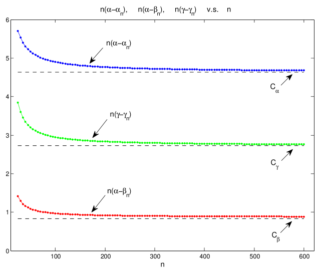
Figure 2: Plot of $n(\alpha-\alpha_{n})$, $n(\alpha-\beta_{n})$, and $n(\gamma-\gamma_{n})$ for $n=25(5)600$ with parameters $w=0.4,k=5,\lambda=8,N=8$.

Table 1: Exact values for $n(\alpha-\alpha_{n})$, $n(\alpha-\beta_{n})$ and $n(\gamma-\gamma_{n})$ and the estimated limits with $k=5,w=0.4,\lambda=8,N=8$

$n$	Unconditional		Conditional
	$n(\alpha-\alpha_{n})$	$n(\alpha-\beta_{n})$	$n(\gamma-\gamma_{n})$
$50$	5.168687891	1.088138412	3.203626718
$100$	4.898446228	0.969210822	2.948216315
$200$	4.764816517	0.917535676	2.832944959
$300$	4.720634969	0.901298885	2.796179050
$400$	4.698621375	0.893353201	2.778092954
$500$	4.685438621	0.888639155	2.767334580
$600$	4.676660628	0.885518032	2.760200812
Limit	$C_{\alpha}$	$C_{\beta}$	$C_{\gamma}$
Estimate	4.6322	0.8297	2.7279
(Std. Err.)	(0.0096)	(0.0167)	(0.0114)

Table 2: The unconditional case

Parameters						$n$			Exact
$\lambda$	$w$	$k$		$25$	$50$	$100$	$200$	$400$	$\alpha$
4	0.2	3	$\alpha_{n}$	0.226474137	0.297081029	0.330413369	0.346549002	0.354481473	0.362322986
			$\alpha-\alpha_{n}$	0.135848849	0.065241957	0.031909617	0.015773984	0.007841513
			$\widetilde{\alpha}_{n}$		0.367687921	0.363745709	0.362684635	0.362413943
			$\alpha-\widetilde{\alpha}_{n}$		$-$0.005364935	$-$0.001422723	$-$0.000361649	$-$0.000090957
			$\beta_{n}$	0.269466265	0.321289109	0.342964036	0.352912780	0.357682871
			$\alpha-\beta_{n}$	0.092856721	0.041033877	0.019358950	0.009410206	0.004640115
			$\widetilde{\beta}_{n}$		0.373111952	0.364638964	0.362861523	0.362452963
			$\alpha-\widetilde{\beta}_{n}$		$-$0.010788966	$-$0.002315978	$-$0.000538537	$-$0.000129977
4	0.2	4	$\alpha_{n}$	0.028528199	0.063252847	0.083861016	0.094813938	0.100432989	0.106139839
			$\alpha-\alpha_{n}$	0.077611640	0.042886992	0.022278823	0.011325901	0.005706850
			$\widetilde{\alpha}_{n}$		0.097977495	0.104469184	0.105766860	0.106052039
			$\alpha-\widetilde{\alpha}_{n}$		0.008162344	0.001670655	0.000372979	0.000087800
			$\beta_{n}$	0.037826080	0.071921990	0.089167692	0.097701122	0.101933685
			$\alpha-\beta_{n}$	0.068313759	0.034217849	0.016972147	0.008438717	0.004206154
			$\widetilde{\beta}_{n}$		0.106017899	0.106413395	0.106234551	0.106166248
			$\alpha-\widetilde{\beta}_{n}$		0.000121940	$-$0.000273556	$-$0.000094712	$-$0.000026409
8	0.4	5	$\alpha_{n}$	0.400190890	0.524770327	0.579159623	0.604320002	0.616397532	0.628144085
			$\alpha-\alpha_{n}$	0.227953195	0.103373758	0.048984462	0.023824083	0.011746553
			$\widetilde{\alpha}_{n}$		0.649349765	0.633548918	0.629480382	0.628475061
			$\alpha-\widetilde{\alpha}_{n}$		$-$0.021205680	$-$0.005404833	$-$0.001336297	$-$0.000330976
			$\beta_{n}$	0.571524668	0.606381317	0.618451977	0.623556407	0.625910702
			$\alpha-\beta_{n}$	0.056619417	0.021762768	0.009692108	0.004587678	0.002233383
			$\widetilde{\beta}_{n}$		0.641237966	0.630522637	0.628660836	0.628264997
			$\alpha-\widetilde{\beta}_{n}$		$-$0.013093881	$-$0.002378552	$-$0.000516751	$-$0.000120912
8	0.4	6	$\alpha_{n}$	0.156407681	0.278520053	0.341202440	0.372097133	0.387351968	0.402452588
			$\alpha-\alpha_{n}$	0.246044907	0.123932535	0.061250148	0.030355455	0.015100620
			$\widetilde{\alpha}_{n}$		0.400632426	0.403884826	0.402991826	0.402606803
			$\alpha-\widetilde{\alpha}_{n}$		0.001820162	$-$0.001432238	$-$0.000539238	$-$0.000154215
			$\beta_{n}$	0.278663391	0.351874806	0.379351117	0.391387631	0.397034846
			$\alpha-\beta_{n}$	0.123789197	0.050577782	0.023101471	0.011064957	0.005417742
			$\widetilde{\beta}_{n}$		0.425086221	0.406827428	0.403424144	0.402682062
			$\alpha-\widetilde{\beta}_{n}$		$-$0.022633633	$-$0.004374840	$-$0.000971556	$-$0.000229474

Table 3: The conditional case

Parameters						$n$			Exact
$w$	$k$	$N$		$25$	$50$	$100$	$200$	$400$	$\gamma$
0.2	4	6	$\gamma_{n}$	0.080688876	0.155913836	0.194799457	0.214242757	0.223935622	0.233600000
			$\gamma-\gamma_{n}$	0.152911124	0.077686164	0.038800543	0.019357243	0.009664378
			$\widetilde{\gamma}_{n}$		0.231138796	0.233685077	0.233686058	0.233628487
			$\gamma-\widetilde{\gamma}_{n}$		0.002461204	$-$0.000085077	$-$0.000086058	$-$0.000028487
		7	$\gamma_{n}$	0.166798419	0.294914521	0.354660825	0.383179030	0.397084766	0.410752000
			$\gamma-\gamma_{n}$	0.243953581	0.115837479	0.056091175	0.027572970	0.013667234
			$\widetilde{\gamma}_{n}$		0.423030623	0.414407129	0.411697234	0.410990502
			$\gamma-\widetilde{\gamma}_{n}$		$-$0.012278623	$-$0.003655129	$-$0.000945234	$-$0.000238502
		8	$\gamma_{n}$	0.291588655	0.469102180	0.542215920	0.575193126	0.590840920	0.605949440
			$\gamma-\gamma_{n}$	0.314360785	0.136847260	0.063733520	0.030756314	0.015108520
			$\widetilde{\gamma}_{n}$		0.646615704	0.615329660	0.608170332	0.606488715
			$\gamma-\widetilde{\gamma}_{n}$		$-$0.040666264	$-$0.009380220	$-$0.002220892	$-$0.000539275
		9	$\gamma_{n}$	0.448718168	0.651907101	0.723414803	0.753448974	0.767220941	0.780225536
			$\gamma-\gamma_{n}$	0.331507368	0.128318435	0.056810733	0.026776562	0.013004595
			$\widetilde{\gamma}_{n}$		0.855096034	0.794922506	0.783483145	0.780992907
			$\gamma-\widetilde{\gamma}_{n}$		$-$0.074870498	$-$0.014696970	$-$0.003257609	$-$0.000767371
0.4	5	6	$\gamma_{n}$	0.162450593	0.224402953	0.254838093	0.269838436	0.277276942	0.284672000
			$\gamma-\gamma_{n}$	0.122221407	0.060269047	0.029833907	0.014833564	0.007395058
			$\widetilde{\gamma}_{n}$		0.286355312	0.285273233	0.284838778	0.284715449
			$\gamma-\widetilde{\gamma}_{n}$		$-$0.001683312	$-$0.000601233	$-$0.000166778	$-$0.000043449
		7	$\gamma_{n}$	0.371395881	0.463718058	0.504028994	0.522865538	0.531971853	0.540876800
			$\gamma-\gamma_{n}$	0.169480919	0.077158742	0.036847806	0.018011262	0.008904947
			$\widetilde{\gamma}_{n}$		0.556040235	0.544339929	0.541702083	0.541078168
			$\gamma-\widetilde{\gamma}_{n}$		$-$0.015163435	$-$0.003463129	$-$0.000825283	$-$0.000201368
		8	$\gamma_{n}$	0.627251924	0.716788906	0.751379277	0.766696715	0.773916208	0.780861440
			$\gamma-\gamma_{n}$	0.153609516	0.064072534	0.029482163	0.014164725	0.006945232
			$\widetilde{\gamma}_{n}$		0.806325887	0.785969648	0.782014154	0.781135700
			$\gamma-\widetilde{\gamma}_{n}$		$-$0.025464447	$-$0.005108208	$-$0.001152714	$-$0.000274260
		9	$\gamma_{n}$	0.864220071	0.918826852	0.936992617	0.944511915	0.947942424	0.951173120
			$\gamma-\gamma_{n}$	0.086953049	0.032346268	0.014180503	0.006661205	0.003230696
			$\widetilde{\gamma}_{n}$		0.973433633	0.955158381	0.952031214	0.951372933
			$\gamma-\widetilde{\gamma}_{n}$		$-$0.022260513	$-$0.003985261	$-$0.000858094	$-$0.000199813

Remark 4.1.

In Tables 1–3, we have taken relatively large values of $w=0.2$ and $0.4$ since the exact unconditional probabilities reported in [21] are less accurate for $w<0.2$. Figure 1 shows that $n(\alpha-\alpha_{n}),n(\alpha-\beta_{n})$ and $n(\gamma^{(N)}-\gamma^{(N)}_{n})$ monotonically approach $C_{\alpha},C_{\beta}$ and $C^{(N)}_{\gamma}$, respectively. In Table 2, $\beta_{n}$ is consistently more accurate than $\alpha_{n}$, which is not surprising since $\alpha_{n}<\min\{\alpha,\beta_{n}\}$. According to Tables 2 and 3, when $n$ doubles, the errors of $\alpha_{n},\beta_{n}$ and $\gamma^{(N)}_{n}$ decrease by roughly a factor of $2$ while the errors of the corrected approximations $\tilde{\alpha}_{n},\tilde{\beta}_{n}$ and $\tilde{\gamma}^{(N)}_{n}$ decrease by (very) roughly a factor of $4$. Thus the corrected approximations are much more accurate than the uncorrected ones. For example, $\tilde{\alpha}_{100}$ and $\tilde{\beta}_{100}$ ($\tilde{\gamma}^{(N)}_{100}$, resp.) are about as accurate as or more accurate than $\beta_{400}$ ($\gamma^{(N)}_{400}$, resp.).

Remark 4.2.

The discrete approximations are usually computed using the Markov chain embedding method. A major drawback of this method is the requirement of a very large state space (corresponding to a large computer memory space) for some practical applications. Indeed, it is shown in [3] that to compute $\alpha_{n},\beta_{n}$ and $\gamma^{(N)}_{n}$ using the Markov chain embedding method, the minimum number of states required is $\binom{nw}{k-1}+1$, which is enormous when $nw$ is large and $k$ is not small. (It should be remarked that [3] is concerned with computation of the reliability for the so-called $d$-within-consecutive-$k$-out-of-$n$ system, which is equivalent to the discrete scan statistic.) The corrected discrete approximations partially alleviate the requirement of large memory space since a reasonable accuracy can be achieved with relatively small $n$.

Remark 4.3.

Since the assumption of constant intensity plays a relatively minor role in the proofs of Theorems 2.1, 2.3 and 3.1, we expect that the method of proof can be extended to the setting of nonhomogeneous Poisson point processes, which is relevant to computation of the power of the continuous scan statistic. In the literature, there appears to be no general method available for computing the exact power under general nonhomogeneous Poisson point processes. The corrected discrete approximations may prove to be useful in such a setting as well as in a multiple-window setting (cf. [23]).

References

- [1] Barton, D.E. and Mallows, C.L. (1965). Some aspects of the random sequence. Ann. Math. Statist. 36, 236–260.
- [2] Chan, H.P. and Zhang, N.R. (2007). Scan statistics with weighted observations. J. Amer. Statist. Assoc. 102, 595–602.
- [3] Chang, J.C., Chen, R.J. and Hwang, F.K. (2001). A minimal-automaton-based algorithm for the reliability of Con(d,k,n) system. Methodol. Comput. Appl. Probab. 3, 379–386.
- [4] Fang, X. and Siegmund, D. (2015). Poisson approximation for two scan statistics with rates of convergence. Ann. Appl. Probab., to appear.
- [5] Fu, J.C. (2001). Distribution of the scan statistic for a sequence of bistate trials. J. Appl. Probab. 38, 908–916.
- [6] Fu, J.C. and Koutras, M.V. (1994). Distribution theory of runs: a Markov chain approach. J. Amer. Statist. Assoc. 89, 1050–1058.
- [7] Fu, J.C. and Wu, T.L. and Lou, W.Y.W. (2012). Continuous, discrete, and conditional scan statistics. J. Appl. Probab. 49, 199–209.
- [8] Glaz, J. and Naus, J.I. (1991). Tight bounds and approximations for scan statistic probabilities for discrete data. Ann. Appl. Probab. 1, 306–318.
- [9] Glaz, J. and Naus, J.I. (2010). Scan statistics. In Methods and Applications of Statistics in the Life and Health Sciences (N. Balakrishnan ed.), 733–747. John Wiley & Sons, New Jersey.
- [10] Glaz, J. and Pozdnyakov, V. and Wallenstein, S. (2009). Scan Statistics: Methods and Applications. Birkhauser, Boston.
- [11] Glaz, J. and Naus, J. and Wallenstein, S. (2001). Scan Statistics. Springer, New York.
- [12] Huntington, R.J. and Naus, J.I. (1975). A simpler expression for Kth nearest neighbor coincidence probabilities. Ann. Probab. 3, 894–896.
- [13] Huffer, F.W. and Lin, C.-T. (1997). Computing the exact distribution of the extremes of sums of consecutive spacings. Comput. Statist. Data Anal. 26, 117–132.
- [14] Huffer, F.W. and Lin, C.-T. (1999). An approach to computations involving spacings with applications to the scan statistic. In Scan Statistics and Applications (J. Glaz and N. Balakrishnan eds.), 141–163. Birkhauser, Boston.
- [15] Hwang, F.K. (1977). A generalization of the Karlin-McGregor theorem on coincidence probabilities and an application to clustering. Ann. Probab. 5, 814–817.
- [16] Janson, S. (1984). Bounds on the distributions of extremal values of a scanning process. Stoch. Proc. Appl. 18, 313–328.
- [17] Karlin, S. and McGregor, G. (1959). Coincidence probabilities. Pacific J. Math. 9, 1141–1164.
- [18] Koutras, M.V. and Alexandrou, V.A. (1995). Runs, scans, and urn model distributions: A unified Markov chain approach. Ann. Inst. Stat. Math. 47, 743–776.
- [19] Loader, C. (1991). Large deviation approximations to the distribution of scan statistics. Adv. Appl. Probab. 23, 751–771.
- [20] Naus, J.I. (1982). Approximations for distributions of scan statistics. J. Amer. Statist. Assoc. 77, 177–183.
- [21] Neff, N.D. and Naus, J.I. (1980). Selected Tables in Mathematical Statistics, Vol. VI. American Mathematical Society, Providence, Rhode Island.
- [22] Siegmund, D. and Yakir, B. (2000). Tail probabilities for the null distribution of scanning statistics. Bernoulli 6, 191–213.
- [23] Wu, T.L., Glaz, J. and Fu, J.C. (2013). Discrete, continuous and conditional multiple window scan statistics. J. Appl. Probab. 50, 1089–1101.