Congestion Dynamics in Pedestrian Single-File Motion

Abstract

This article considers execution and analysis of laboratory experiments of pedestrians moving in a quasi-one-dimensional system with periodic boundary conditions. To analyze characteristics of jams in the system we aim to use the whole experimental setup as the measurement area. Thus the trajectories are transformed to a new coordinate system. We show that the trajectory data from the straight and curved parts are comparable and assume that the distributions of the residuals come from the same continuous distribution. Regarding the trajectories of the entire setup, the creation of stop-and-go waves in pedestrian traffic can be investigated anddescribed.

1 Introduction

In recent years many research groups have executed experiments with pedestrians, see e.g. Hoogendoorn2003 ; Seyfried2005 ; Chattaraj2009 ; Jelic2012 ; Yanagisawa2012 . One phenomenon which can be observed is a stop-and-go wave well known from vehicular traffic, e.g., Chowdhury2000 . It is visible in the simplest system with a one-dimensional movement of pedestrians along a line with closed boundary conditions, e.g., for a ring Seyfried2005 and for a circle Jelic2012 .

In the following we summarize previous work on one-dimensional pedestrian movements where stop-and-go waves were analyzed. Seyfried2005 executed the first one-dimensional experiments in 2005. For the first time high densities were examined in Portz2010 and the existence of stop-and-go waves in pedestrian traffic was shown. In Portz2010 also an adaptive velocity model with reaction time was proposed, which is able to reproduce qualitatively similar stop-and-go waves as they are observable in the experimental data, see Seyfried2010 . A coexistence of two differing speed phases in this data was shown in Portz2011 by analyzing the fundamental diagram in specific density regions. A model that reproduces this coexistence was also proposed. The same experimental data was taken in Eilhardt2014 to test a stochastic headway dependent velocity model. Jelic2012 compared data from a circle with data from a straight line. Beside the free flow and congested regime of the fundamental diagram they found a third regime named weakly constrained regime. This regime lies between the free and the strongly congested regime.

In Seyfried2010 , the measurement section of the nearly $27$ m corridor with closed boundary conditions covers $4$ m only. This restriction makes it impossible to test models concerning number and dimension of a stop-and-go wave because of lack of data. A second restriction is the duration of an experiment run. In experiments, the duration may be too short to reach a stable state. That is why the lifetime of a stop-and-go wave, its length in space and the number of stop-and-go waves in the system cannot be observed.

In this article we want to handle this problem. Experiments where the whole system was observed are analyzed. Furthermore, we introduce a methodology to analyze characteristics of stop-and-go waves.

2 Experiments

Laboratory experiments were performed within the framework of the project BaSiGo in June 2013. The aim of those experiments is a better understanding of pedestrian dynamics in critical crowded states, e.g., in front of an entrance to a concert hall, thus in high densities. It included large-scale experiments in various scenarios with up to 1000 pedestrians per run during five days. The probands were mostly students ($55\%$ male and $45\%$ female) at the age of 18 to 72 years, $25$ years on average, with an average height of $1.71$ m and recieved 50 Euro per day. $13\%$ of them were living in suburbs or rural areas and $68\%$ in cities or major cities.

2.1 Experimental setup

One-dimensional laboratory experiments for pedestrians in a system with periodic boundary conditions were executed. The setup is a ring corridor with a circumference about $C=26.5$ m ($r_{0}=3$ m, $l=4$ m). Six runs were performed withdifferent number of participants ($N=15,\,30,\,47,\,55,\,52,\,59$) so that the global density ($\rho_{g}=N/C$) ranges from $0.57$ to $2.27$ Ped/m. For each run, the pedestrians initially are arranged uniformly in the setup. Then there are two commands, the first to start walking with normal speed in the corridor and the second for stopping.

2.2 Data collection

To enable the automatic tracking of the trajectories, the pedestrians wear hats with a marker. For each run the whole setup was recorded from the top video camera with a frame rate of $16$ fps. From those video recordings pedestrian trajectories who are describing the movement of the heads of the pedestrians were extracted. For more details to this method we refer toMehner2015 in these proceedings. Fig. 1 shows the trajectories for the runs with $N=15$ and $N=59$ which leads to the global density $0.57$ Ped/m and $2.27$ Ped/m, respectively.

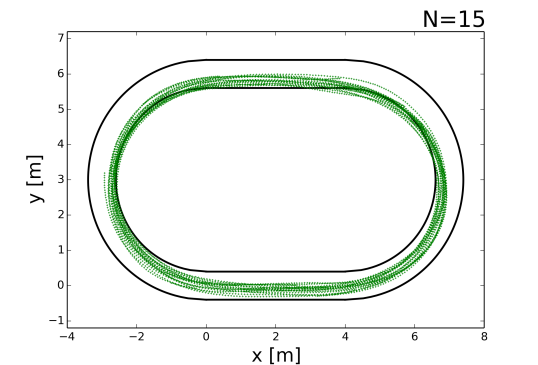
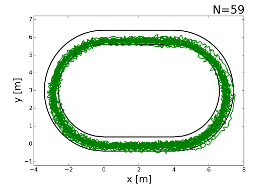
Figure 1: Extracted trajectories for $N=15$ and $N=59$

2.3 Data preparation

We want to study one-dimensional characteristics of stop-and-go waves. Therefore, we introduce a coordinate $\hat{x}$ along the ring which corresponds to the distance from the origin measured along the middle line of the corridor. It corresponds to the walking distance of a person staying always in the middle. The coordinate $\hat{y}$ is always perpendicular to the $\hat{x}$-axis. It measures the deviation from the center of the corridor, see Fig. 2. We call $\hat{x}$ the main position and $\hat{y}$ the orientated distance.

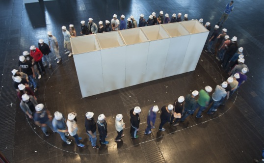
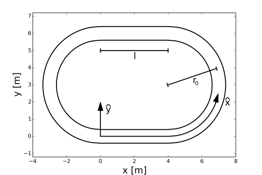
Figure 2: Left: Photo from the experiment by Marc Strunz. Right: New coordinate system $\hat{x}$, $\hat{y}$

The transformation $\lambda:\mathbb{R}^{2}\rightarrow\mathbb{R}^{2}$, $\left(\begin{array}[]{c}x\\ y\end{array}\right)\mapsto\left(\begin{array}[]{c}\hat{x}\\ \hat{y}\end{array}\right)$ is described by:

$$\hat{y}=\left\{\begin{array}[]{ll}\sqrt{x^{2}+(y-r_{0})^{2}}-r_{0}&\quad x<0,\\ \sqrt{(y-r_{0})^{2}}-r_{0}&\quad 0\leq x\leq l,\\ \sqrt{(x-l)^{2}+(y-r_{0})^{2}}-r_{0}&\quad x>l,\end{array}\right.$$ (4)

$$\hat{x}=\left\{\begin{array}[]{ll}2l+r_{0}\pi+r_{0}\arccos(\frac{r_{0}-y}{\sqrt{(x-l)^{2}+(y-r_{0})^{2}}})&\quad x<0,\\ x&\quad 0\leq x\leq l,~{}y<r_{0},\\ 2l+r_{0}\pi-x&\quad 0\leq x\leq l,~{}y\geq r_{0},\\ l+r_{0}\arccos(\frac{r_{0}-y}{\sqrt{x^{2}+(y-r_{0})^{2}}})&\quad x>l.\end{array}\right.$$ (9)

Fig. 3 shows the trajectories of adjusted data in the new coordinate system for two runs. The straight lines in the ring correlate to the intervals $[0,4]$ m and $[14.42,18.42]$ m of the main position. Just as well the two other intervals correlate to the two curved parts. In the following, we will only examine the main position, described by Eq. 9 and omit the orientated distance. That means that all further calculations come from this one-dimensional main position.

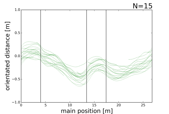
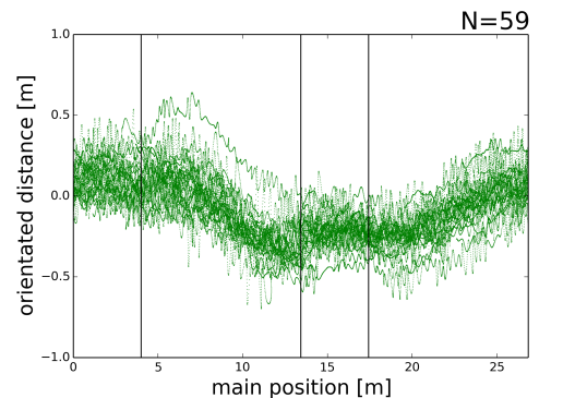
Figure 3: Adjusted trajectories for $N=15$ and $N=59$ in the new coordinate system

3 Results

In this section we test whether the fundamental diagram has different properties in the straight and curved part of the corridor, i.e. whether it is influenced by the curvature.

3.1 Curvature-dependence of the fundamental diagram

The ring corridor, our experimental setup, has four parts, twice the straight line and twice the half circle. Fig. 4 shows the Voronoi-based fundamental diagram for pedestrians moving in the straight line and in the curve. To distinguish between the six runs, each run has a separate symbol and color.

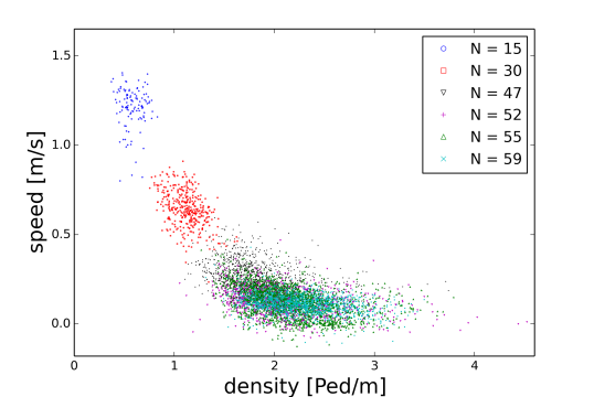
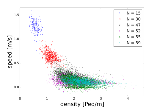
Figure 4: The fundamental diagram of single file pedestrian motion. Left: Data from the straight part. Right: Data from the curved part

The speed of pedestrian $i$ at time $t$ is calculated by the position difference over half a second divided by the time $v_{i}(t)=(\hat{x}_{i}(t+\Delta t)-\hat{x}_{i}(t-\Delta t))/(2\Delta t)$ with$\Delta t=0.25$ s. The density is then $\rho_{i}(t)={d_{i}}^{-1}$, where the Voronoi space $d_{i}$ of pedestrian $i$ is half the distance between the two neighbors $i-1$ and $i+1$,$d_{i}=(\hat{x}_{i-1}-\hat{x}_{i+1})/2$.

For analyzing the characteristics of stop-and-go waves in the whole system we want to combine the data of both parts. First of all we test the comparability of the fundamental diagram for the straight line and the curve. That means we study the distribution for both parts. The Kolmogorov-Smirnov test gives an indication whether two data clouds have the same distribution or not. A precondition for this test is that the data has to be independent, which can be shown with the autocorrelation.

We use two clouds with 3000 independent data points of each category, see Fig. 5 on the left side. The autocorrelation was tested for those data points to ensure that the observations are independent. An exponential function $f$ for the shape of the speed according to the density is fitted by least square. The distributions of the residuals for the clouds are tested with the Kolmogorov-Smirnov test. The null hypothesis is H0: ’the distribution is the same for the two samples’. The frequency of residuals for both parts is shown in Fig. 5, right. With $p=0.791$ we can clearly not reject the assumption that the distributions of the residuals come from the same continuous distribution.

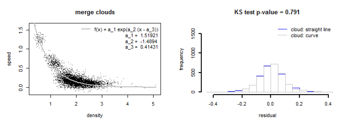
Figure 5: Left: Fundamental diagram of single file pedestrian motion for 6000 data points and its fitted exponential function. Right: Result of the Kolmogorov-Smirnov test

With the Kolmogorov-Smirnov test we have shown that the density speed relation in the straight line is subject to the distribution of the density speed relation in the curve. That means that curvature effects on the fundamental diagram can be neglected.

3.2 Visualization of stop-and-go waves

To visualize stop-and-go waves, we use the knowledge that there is a coexistence of two separate speed phases. The fundamental diagram for the whole system for all six runs is shown in Fig. 6 on the left side. By analyzing the frequency of speeds in specific density regions the coexistence of two differing speed regimes can be identified. One peak is around the speed $0.12$ m/s and the other one around $0$ m/s. Negative speeds result from the swaying of heads of standing pedestrians.

In order to distinguish both phases, we introduce a stop speed $v_{stop}$. Standing pedestrians have a speed lower than this stop speed and moving pedestrians have a speed which is higher than the stop speed. We set the stop speed to $v_{stop}=0.05$ m/s, which appears to be a reasonable value for our experiments. We have to note, that this value is not fixed and there might be better ones for other experiments.

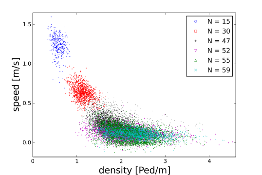
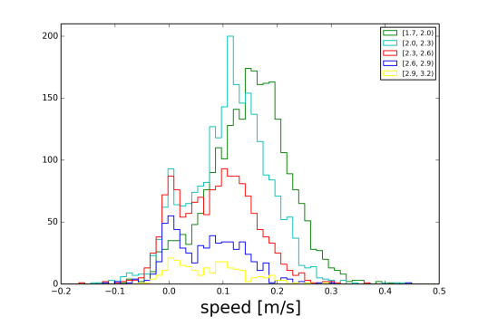
Figure 6: Left: Fundamental diagram of single file pedestrian motion. Right: Frequency of speed for certain density regions, $N=55$

3.3 Stop-and-go waves

We define a stop-and-go wave by a consecutive sequence of one or more standing pedestrians. Fig. 7 shows the main positions of the pedestrians for one minute for four different runs. The plotted positions have a length of $0.2$ m to represent a body length. Pedestrians in a stop wave are marked in red. With 15 pedestrians in the system, no stopping occurs whereas 52, 55 or 59 pedestrians generate stop-and-go waves. Eye-catching is the run with 55 pedestrians. Long and big stop-and-go waves can be observed. The duration of the experiment run was too short to judge whether the regarded time interval represents a stable state.

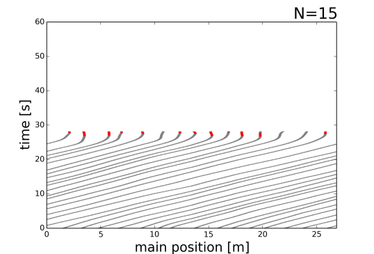
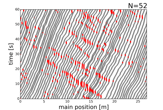
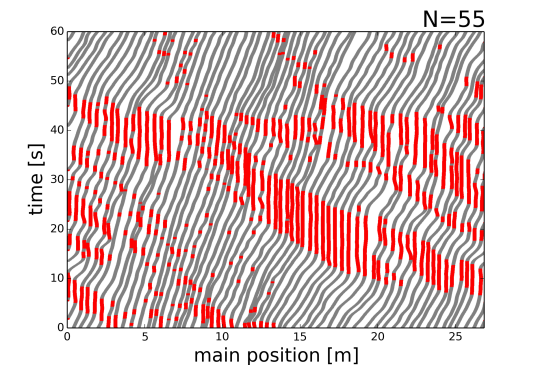
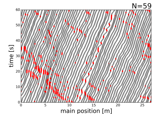
Figure 7: Trajectories of the main positions depending on time, $N=15,\,52,\,55,\,59$. A red dot indicates a pedestrian in a congestion, that means he has a speed not higher than the stop speed

A stop wave can be characterized by the number of pedestrians in this region at a certain time, by the length in space at a certain time and by the duration at a certain time and position. The length of a stop wave can be described by the number of standing pedestrians in a line or the distance between the first standing pedestrian and the last one. Higher densities lead to stop waves with more standing pedestrians than lower densities whereas the average length of a stop wave gets shorter. The duration of a stop wave can be described by the time while the first pedestrian in this stop wave is standing and the last standing pedestrian starts to move.

In the run $N=52$, all stop waves have nearly the same speed around $-0.5$ m/s. The run $N=59$ has lower speeds of stop waves around $-0.32$ m/s.

4 Conclusion

We extracted pedestrian trajectories from the whole setup of a ring experiment. This data was transformed to a quasi-one-dimensional straight line. The resulting fundamental diagram for the straight and curved part have the same shape and are comparable, tested with the Kolmogorov-Smirnov test. The fundamental diagram of both parts shows a coexistence of two differing speed zones in specific density regions. A stop speed was introduced to distinguish between moving and standing pedestrians. Standing pedestrians define a stop wave that can be described by the characteristics length and duration. While the maximum number of pedestrians in a stop wave in our data is increasing with growing density, the average length decreases. In the future, we want to analyze those characteristics in a quantitative way.

- (1) Chattaraj, U., Seyfried, A., Chakroborty, P.: Comparison of pedestrian fundamental diagram across cultures. Advances in Complex Systems 12(3), 393–405 (2009)
- (2) Chowdhury, D., Santen, L., Schadschneider, A.: Statistical physics of vehicular traffic and some related systems. Physics Reports 329(4–6), 199–329 (2000)
- (3) Eilhardt, C., Schadschneider, A.: Stochastic headway dependent velocity model for 1d pedestrian dynamics at high densities. Transportation Research Procedia 2(0), 400–405 (2014)
- (4) Hoogendoorn, S.P., Daamen, W., Bovy, P.H.L.: Microscopic pedestrian traffic data collection and analysis by walking experiments: Behaviour at bottlenecks. In: E.R. Galea (ed.) Pedestrian and Evacuation Dynamics 2003, pp. 89–100. CMS Press, London (2003)
- (5) Jelić, A., Appert-Rolland, C., Lemercier, S., Pettré, J.: Properties of pedestrians walking in line: Fundamental diagrams. Physical Review E E 85(85), 9 (2012)
- (6) Mehner, W., Boltes, M., Seyfried, A.: Methodology for generating individualized trajectories from experiments. In these proceedings
- (7) Portz, A., Seyfried, A.: Modeling stop-and-go waves in pedestrian dynamics. In: R. Wyrzykowski, J. Dongarra, K. Karczewski, J. Wasniewski (eds.) PPAM 2009, Part II, pp. 561–568. Springer-Verlag Berlin Heidelberg (2010)
- (8) Portz, A., Seyfried, A.: Analyzing stop-and-go waves by experiment and modeling. In: R. Peacock, E. Kuligowski, J. Averill (eds.) Pedestrian and Evacuation Dynamics 2010, pp. 577–586. Springer (2011)
- (9) Seyfried, A., Boltes, M., Kähler, J., Klingsch, W., Portz, A., Rupprecht, T., Schadschneider, A., Steffen, B., Winkens, A.: Enhanced empirical data for the fundamental diagram and the flow through bottlenecks. In: W.W.F. Klingsch, C. Rogsch, A. Schadschneider, M. Schreckenberg (eds.) Pedestrian and Evacuation Dynamics 2008, pp. 145–156. Springer-Verlag Berlin Heidelberg (2010)
- (10) Seyfried, A., Steffen, B., Klingsch, W., Boltes, M.: The fundamental diagram of pedestrian movement revisited. J. Stat. Mech. P10002 (2005)
- (11) Yanagisawa, D., Tomoeda, A., Nishinari, K.: Improvement of pedestrian flow by slow rhythm. Physical Review E 85, 016,111 (2012)