Extrinsic and intrinsic curvatures in thermodynamic geometry

Abstract

We investigate the intrinsic and extrinsic curvature of a certain hypersurface in thermodynamic geometry of a physical system and show that they contain useful thermodynamic information. For an anti-Reissner-Nordström-(A)de Sitter black hole (Phantom), the extrinsic curvature of a constant $Q$ hypersurface has the same sign as the heat capacity around the phase transition points. The intrinsic curvature of the hypersurface can also be divergent at the critical points but has no information about the sign of the heat capacity. Our study explains the consistent relationship holding between the thermodynamic geometry of the KN-AdS black holes and those of the RN ($J$-zero hypersurface) and Kerr black holes ($Q$-zero hapersurface) ones ref1 . This approach can easily be generalized to an arbitrary thermodynamic system.

I Introduction

Bekenstein and Hawking showed that a black hole has a behavior similar to a common thermodynamic system ref2 ; ref3 . They drew a parallel relationship between the four laws of thermodynamics and the physical properties of black holes by considering the surface gravity and the horizon area as the temperature and entropy, respectively ref4 . An interesting topic is to study phase transitions in black hole thermodynamics where the heat capacity diverges ref5 ; ref6 . These divergence points of heat capacity are usually associated with a second order phase transition for some fixed black hole parameters ref24 .

Geometric concepts can also be used to study the properties of an equilibrium space of thermodynamic systems. Riemannian geometry in the space of equilibrium states was introduced by Weinhold ref8 and Ruppeiner ref9 ; ref10 who defined metric elements as the Hessian matrix of the internal energy and entropy. These geometric structures are used to find the significance of the distance between equilibrium states. Consequently, various thermodynamic properties of the system can be derived from the properties of these metrics, especially critical behaviors, and stability of various types of black hole families ref11 ; ref12 ; ref13 . For the second order phase transitions, Ruppeiner curvature scalar (R) is expected to diverge at critical points ref14 ; ref24 ; ref15 ; ref16 ; ref17 . Due to the success of this geometry to identify a phase transition, several works ref18 ; ref19 ; ref20 ; ref21 have exploited it to explain the black hole phase transitions.

The Ruppeiner geometry has also been analyzed for several black holes to find out the thermodynamic properties ref22 ; ref23 . As a result, the Ruppeiner curvature is flat for the BTZ and Reissner-Nordström (RN) black holes, while curvature singularities occur for the Reissner-Nordström anti de Sitter (RN-AdS) and Kerr black holes. Moreover, it has been argued in ref1 that all possible physical fluctuations could be considered for calculating curvature because neglecting one parameter may lead to inadequate information about it. Therefore, the thermodynamic curvature of RN should be reproduced from the Kerr-Newmann anti-de Sitter (KN-AdS) black hole when the angular momentum $J\to 0$ and cosmological constant $\Lambda\to 0$. This approach leads to a non-zero value for the Ruppeiner scalar, which is in contrast to the reports on RN in pervious works ref22 ; ref23 .

The present letter seeks to explain this contrast by obtaining intrinsic and extrinsic curvatures of the related submanifolds. The induced metric (intrinsic curvature) and the extrinsic curvature of a constant $J$ hypersurface contain the necessary information about the properties of this hypersurface. The zero limit of an angular momentum for a KN-AdS black hole is equivalent to the two-dimensional constant J hypersurface embedded in a three-dimensional complete thermodynamic space. The curvature scalar of KN-AdS black hole on this hypersurface can be decomposed into an intrinsic curvature (Ruppeiner curvature of RN black hole), which is zero, and an extrinsic part that give the curvature singularities.

We also prove that there is a one-to-one correspondence between divergence points of the heat capacities and those of the extrinsic curvature for thermodynamic descriptions where potentials are related to the mass (rather than the entropy) by Legendre transformations. In spite of this correspondence, we can get other information about thermodynamics like stability and non-stability regions around phase transitions from singularities of extrinsic curvature and certain elements of the Ricci tensor.

The organization of the letter is as follows. In Section II and III, we analyze the nature of the phase transition through the diagrams of the Riemann tensor elements and extrinsic curvature. In Section IV, we try to provide an answer to the question arising from the article ref1 , ” Ruppeiner geometry of RN black holes: flat or curved?” using the concept of thermodynamic hypersurface in lower dimensions. In Section V, we consider a Pauli paramagnetic gas and investigate a hypersurface in its thermodynamic geometry that corresponds to a zero magnetic field. Section VI contains a discussion of our results.

II Thermodynamic extrinsic curvature

We begin with a review of our previous results on the correspondence between second order phase transitions and singularities of the thermodynamic geometry ref20 ; ref21 . We also introduce extrinsic curvature as a new concept of the thermodynamic geometry. We will use this quantity in determining some information about stability and non-stability regions around phase transitions. For charged black holes, a specific heat at a fixed electric charge is defined as follows:

$${{C}_{Q}}=T{{\left(\frac{\partial S}{\partial T}\right)}_{Q}}=Tdet\left[\frac{\partial(S,Q)}{\partial{(T,Q)}}\right]=\frac{T{{\left\{S,Q\right\}}_{S,Q}}}{{{\left\{T,Q\right\}}_{S,Q}}}$$ (1)

It is obvious that the phase transitions of ${{C}_{Q}}$ are the zeros of ${{\left\{T,Q\right\}}_{S,Q}}$ (Appx. A may be consulted for a brief introduction to the bracket notation). Moreover, the Ruppeiner metric in the mass representation can be expressed as:

$${\textbf{g}}^{R}=\frac{H_{i,j}{M}}{T}$$ (2)

where $H_{i,j}M=\left({{{\partial}^{2}}{M}}/{\partial{{X}^{i}}\partial{{X}^{j}}}\right)$ is called the Hessian matrix and ${{X}^{i}}=(S,Q)$ are extensive parameters. Therefore, according to the first law of thermodynamics, ${dM}={TdS+{\Phi}dQ}$, one could define the denominator of the scalar curvature $R(S,Q)$ by:

$$g=det({\textbf{g}}^{R})=det\left[\frac{\partial(T,\Phi)}{T\partial{(S,Q)}}\right]=\frac{{{\left\{T,\Phi\right\}}_{S,Q}}}{{{T}^{2}}}=\frac{1}{T{{C}_{\Phi}}{{C}_{S}}}$$ (3)

where, ${{C}_{S}}\equiv{{\left({\partial Q}/{\partial\Phi}\right)}_{S}}$ and,

$${{C}_{\Phi}}=T{{\left(\frac{\partial S}{\partial T}\right)}_{\Phi}}=\frac{T{{\left\{S,\Phi\right\}}_{S,Q}}}{{{\left\{T,\Phi\right\}}_{S,Q}}}$$ (4)

As a result, the scalar curvature $R(S,Q)$ is not able to explain the properties of the phase transitions of $C_{Q}$. From Eq. (3), it is obvious that the phase transitions of ${{C}_{\Phi}}$ correspond precisely to the singularities of $R(S,Q)$. Now, one is able to prove an exact correspondence between singularities of this new metric $(\bar{R}(S,\Phi))$ and phase transitions of $C_{Q}$ ref20 by redefining the Ruppeiner metric as follows:

$$\overline{\textbf{{g}}}=\frac{H_{i,j}{\overline{M}}}{T}$$ (5)

where, $\overline{M}(S,\Phi)=M(S,Q)-\Phi Q$ is the enthalpy potential for $M(S,Q)$ and ${{X}^{i}}=(S,\Phi)$. From the first law, ${d\overline{M}}(S,\Phi)=TdS-\Phi dQ$, the denominator of $\overline{R}(S,\Phi)$ is obtained by:

$$\overline{g}=det({\overline{\textbf{g}}})=det\left[\frac{\partial(T,-Q)}{T\partial{(S,\Phi)}}\right]=-\frac{1}{{{T}^{2}}}{{\left\{T,Q\right\}}_{S,\Phi}}=-\frac{C_{S}}{TC_{Q}}$$ (6)

It is straightforward to show that the phase transitions of ${{C}_{Q}}$ are equal to the singularities of $\overline{R}(S,\Phi)$. We now examine a relationship between the divergences of the extrinsic curvature and the phase transition points. As already mentioned, the extrinsic curvature can be constructed by living on a certain hypersurface with a normal vector (See Appx. B). Since the heat capacity, $C_{Q}$, is defined at a constant electric charge, we should set on a constant $Q$ hypersurface. To do this, we change the coordinate from $(S,\Phi)$ to $(S,Q)$ by using the following Jacobian matrix.

$$\textbf{J}\equiv\frac{\partial\left(S,\Phi\right)}{\partial\left(S,Q\right)}$$ (7)

The metric elements of ${\overline{M}}(S,\Phi)$ in the new coordinate $(S,Q)$ can also be changed as follows:

$$\overline{g}_{ij}^{\prime}=J_{ik}^{T}\,\ \overline{g}_{kl}\,\ {{J}_{lj}}$$ (8)

where, $J^{T}$ is the transpose of $J$. One can also rewrite Eq. (5) as a Jacobian matrix by:

$$\overline{\textbf{g}}=\frac{\partial\left(T,-Q\right)}{T\partial\left(S,\Phi\right)}$$ (9)

Thus, the new metric takes the following form:

$${{\bar{{\textbf{g}}^{\prime}}}} = {{\left(\frac{\partial\left(S,\Phi\right)}{\partial\left(S,Q\right)}\right)}^{T}}\left(\frac{\partial\left(T,-Q\right)}{T\partial\left(S,\Phi\right)}\right)\left(\frac{\partial\left(S,\Phi\right)}{\partial\left(S,Q\right)}\right)$$ (10)

$$= {{\left(\frac{\partial\left(S,\Phi\right)}{\partial\left(S,Q\right)}\right)}^{T}}\left(\frac{\partial\left(T,-Q\right)}{T\partial\left(S,Q\right)}\right)$$

Furthermore by regarding, given the property of the determinant, i.e., $det(J^{T})=det(J)$, the determinant of the above relation can be calculated as follows:

$$\bar{{{g}}^{\prime}}=\det\left({{\left(\frac{\partial\left(S,\Phi\right)}{\partial\left(S,Q\right)}\right)}^{T}}\left(\frac{\partial\left(T,-Q\right)}{\partial\left(S,Q\right)}\right)\right)=$$

$$\det\left(\frac{\partial\left(S,\Phi\right)}{\partial\left(S,Q\right)}\right)\det\left(\frac{\partial\left(T,-Q\right)}{\partial\left(S,Q\right)}\right)=-\frac{{{C}_{S}}^{-1}}{T{{C}_{Q}}}$$ (11)

On the other hand, when we restrict ourselves to live on the constant $Q$ hypersurface with a normal vector ${{\overline{n}}_{Q}}=-1/\sqrt{\left|{{\overline{g}}^{\prime QQ}}\right|}$, the extrinsic curvature will be given by:

$$\overline{K}(S,Q)=\frac{1}{2\bar{g^{\prime}}}\left[\left({{\overline{n}}^{\mu}}{{\partial}_{\mu}}\right)\bar{g^{\prime}}\right]+\left({{\partial}_{\mu}}{{\overline{n}}^{\mu}}\right)$$ (12)

where, ${{\overline{n}}^{\mu}}=\left({{\overline{n}}^{S}},{{\overline{n}}^{Q}}\right)=\left({{\overline{g^{\prime}}}^{SQ}},{{\overline{g^{\prime}}}^{QQ}}\right){{\overline{n}}_{Q}}$ (See Appx. B). From Eq. (10), the metric tensor in the new coordinate can be calculated as follows:

$${{\bar{{\textbf{g}}^{\prime}}}}=diag(C_{Q}^{-1},-\frac{C_{S}^{-1}}{T})$$ (13)

Therefore, on the constant $Q$ hypersurface, we have:

$${{\overline{n}}^{\mu}}=\left(0,{{\overline{n}}^{Q}}\right)=\left(0,\sqrt{\left|T{{C}_{S}}\right|}\right)$$ (14)

It is easy to show that the above vector is a normalized vector ($\bar{n}_{\mu}\bar{n}^{\mu}=-1$). Therefore, the extrinsic curvature can be rewritten as follows:

$$\bar{K}={{\left.\frac{T{{C}_{Q}}}{{{C}_{S}^{-1}}}\left[\sqrt{\left|T{{C}_{S}}\right|}{{\partial}_{Q}}\left(\frac{{{C}_{S}^{-1}}}{T{{C}_{Q}}}\right)\right]+{{\partial}_{Q}}\sqrt{\left|T{{C}_{S}}\right|}\right|}_{Q=cte}}$$ (15)

Indeed this relation tells us that the singularities of this curvature occur exactly at phase transitions of the $C_{Q}$. It should be noted that in this case when the extrinsic curvature diverges, the metric components are differentiable. However, the metric elements are non-differentiable for extremal black holes in the Ruppeiner geometry. Our study indicates that in thermodynamic geometry divergences of the extrinsic curvature does not always implies non-differentiavble metric elements. In table I, we compare the heat capacity and the extrinsic curvature function for $Kerr$, $RN$, $BTZ$, and Einstein-Maxwell-Gauss-Bonnet ($EMGB$) Ref6 black holes. In all cases, the roots of the extrinsic curvature denominator show phase transition points. The extrinsic curvature also changes its sign at the phase transition points which is exactly a similar behavior to heat capacity. Generally, for thermodynamic systems with $(n+1)$ variables, one could consider the following metric,

$$\overline{\textbf{g}}=\frac{H_{i,j}\overline{M}}{T}=\frac{\partial\left(T,-Q_{1},-Q_{2},...,Q_{n}\right)}{T\partial\left(S,\Phi_{1},\Phi_{2},...,\Phi_{n}\right)}$$ (16)

where $\overline{M}=M-\sum_{i}^{n}\Phi_{i}Q_{i}$ and $X^{i}=\left(S,Q_{1},...,Q_{n}\right)$. Furthermore, $\left(T,\Phi_{1},...,\Phi_{n}\right)$ are called extensive parameters. Then utilizing the Jacobian matrix as follows:

$$\textbf{J}\equiv\frac{\partial\left(S,\Phi_{1},\Phi_{2},...,\Phi_{n}\right)}{\partial\left(S,Q_{1},Q_{2},...,Q_{n}\right)}$$ (17)

in a similar way, the metric tensor can be represented by below block-diagonal matrix.

$$\bar{{{\textbf{g}}}^{\prime}}=diag(C_{Q_{1},Q_{2},...,Q_{n}}^{-1},-\textbf{G})$$ (18)

where $G$ is a square matrix of order $n$ defined by the following relation,

$$\textbf{G}=\frac{H_{i,j}{M}}{T}\,\ ;\,\ X^{i}=(Q_{1},Q_{2},...,Q_{n})$$ (19)

Thus the metric determinant in the new coordinates can be written as:

$$\bar{{{g}}^{\prime}}=\frac{\left[C_{S,Q_{1},Q_{2},...,Q_{n}}C_{S,\Phi_{1},Q_{2},...,Q_{n}}...C_{S,\Phi_{1},\Phi_{2},...,\Phi_{n}}\right]^{-1}}{{(-T)}^{n}C_{Q_{1},Q_{2},...,Q_{n}}}$$ (20)

where above functions were defined in ref20 . Now, a constant $Q_{i}$ hypersurface has the following unit normal vector,

$$\bar{n}_{\mu}=(0,0,...,-{(TC_{S,\Phi_{1},...,\Phi_{i-1},\Phi_{i+1},...,\Phi_{n}})^{\frac{-1}{2}}},..,0)$$ (21)

where the non-zero term places in $i^{th}$ column. The extrinsic curvature, $\bar{K}(S,Q_{1},Q_{2},...,Q_{n})$, can be calculated using Eq (71). It is interesting that the extrinsic curvature has the same behavior as the specific heat, $C_{Q_{1},Q_{2},...,Q_{n}}$.

For a Kerr-Newman ($KN$) black hole with the following mass,

$$M=\frac{\sqrt{S(4{{J}^{2}}+{{S}^{2}}+2{{Q}^{2}}S+{{Q}^{4}})}}{2S}$$ (22)

metric elements are defined as follows:

$$\overline{\textbf{g}}=\frac{H_{i,j}\overline{M}}{T}=\frac{\partial\left(T,-Q,-J\right)}{T\partial\left(S,\Phi,\Omega\right)}$$ (23)

where $T$ is the Hawking temperature, $\Omega$ is the angular velocity, and $\Phi$ is the potential deference ref20 ; ref21 . When somebody restricts himself to live on the constant $J$ hypersurface which has the orthogonal normal vector, ${{\overline{n}}_{J}}=-1/\sqrt{\left|{TC_{S,\Phi}}\right|}$, the extrinsic curvature diverges at the phase transition point and exhibit a similar sign behavior around the transition points. In Figure 1, the graph of the extrinsic curvature, $\overline{K}$, and the heat capacity, $C_{J,Q}$, for the Kerr-Newman black hole ($KN$) shows an exact correspondence between singularities and phase transitions (Note that the first divergence point is related to $T=0$.). It is surprising that the same result obtains by considering a constant $Q$ hypersurface with unit normal vector, ${{\overline{n}}_{Q}}=-1/\sqrt{\left|{TC_{S,\Omega}}\right|}$. Moreover, it will be easy to show that the signs of such Ricci tensor elements as $\overline{R}_{SS}$, $\overline{R}_{SQ}$ and $\overline{R}_{SJ}$ are similar to that of the $C_{J,Q}$ around the transition points.

$kerr$	$RN$
$M(S,J)=\frac{\sqrt{{\frac{S}{\pi}}+4\,{\frac{{J}^{2}\pi}{S}}}}{2}$	$M(S,Q)=\frac{\sqrt{S\pi}\left({\pi}^{-1}+{\frac{{Q}^{2}}{S}}\right)}{2}$
$T(S,J)=-{\frac{4\,{J}^{2}{\pi}^{2}-{S}^{2}}{4\sqrt{\pi}{S}^{2}}{\frac{1}{\sqrt{{\frac{4\,{J}^{2}{\pi}^{2}+{S}^{2}}{S}}}}}}$	$T(S,Q)=-{\frac{\sqrt{S\pi}{Q}^{2}}{2{S}^{2}}}$
$\overline{K}(S,J)={\frac{2J\pi\,\left(48\,{J}^{4}{\pi}^{4}+8\,{J}^{2}{\pi}^{2}{S}^{2}+3\,{S}^{4}\right)\sqrt{2}\sqrt{S}}{\left(48\,{J}^{4}{\pi}^{4}+24\,{J}^{2}{\pi}^{2}{S}^{2}-{S}^{4}\right)\sqrt{16\,{J}^{4}{\pi}^{4}-{S}^{4}}}}$	$\overline{K}(S,Q)=0$
$C_{J}(S,J)=-{\frac{2S\left(16\,{J}^{4}{\pi}^{4}-{S}^{4}\right)}{48\,{J}^{4}{\pi}^{4}+24\,{J}^{2}{\pi}^{2}{S}^{2}-{S}^{4}}}$	$C_{Q}(S,Q)=-S/2$
$BTZ$	$EMGB$
$M(S,J)={\frac{{S}^{2}}{16{\pi}^{2}{l}^{2}}}+4\,{\frac{{\pi}^{2}{J}^{2}}{{S}^{2}}}$	$M(S,Q)=\pi\alpha+{\frac{\pi\,{Q}^{2}}{6\sqrt[3]{{S}^{2}}}}+{\pi}^{2}\sqrt[3]{{S}^{2}}-\frac{\pi\,\Lambda\,\sqrt[3]{{S}^{4}}}{12}$
$T(S,J)={\frac{S}{8{\pi}^{2}{l}^{2}}}-8\,{\frac{{\pi}^{2}{J}^{2}}{{S}^{3}}}$	$T(S,Q)=-{\frac{\pi\,\left(\Lambda\,{S}^{4}\sqrt[3]{{S}^{2}}-6\,\pi\,\left({S}^{2}\right)^{2/3}\left({S}^{4}\right)^{2/3}+{Q}^{2}\left({S}^{4}\right)^{2/3}\right)}{9S\sqrt[3]{{S}^{2}}\left({S}^{4}\right)^{2/3}}}$
$\overline{K}(S,J)={\frac{32{S}^{7/2}J{\pi}^{2}l}{\left(192\,{J}^{2}{\pi}^{4}{l}^{2}+{S}^{4}\right)\sqrt{64\,{J}^{2}{\pi}^{4}{l}^{2}-{S}^{4}}}}$	$\overline{K}(S,Q)={\frac{2Q{S}^{3/2}\left(\Lambda\,{S}^{2/3}-4\,\pi\right)\sqrt{3}}{\left(\Lambda\,{S}^{8/3}-5\,{Q}^{2}{S}^{2/3}+6\,\pi\,{S}^{2}\right)\sqrt{\Lambda\,{S}^{2}-6\,\pi\,{S}^{4/3}+{Q}^{2}}}}$
$C_{J}(S,J)=-{\frac{\left(64\,{J}^{2}{\pi}^{4}{l}^{2}-{S}^{4}\right)S}{192\,{J}^{2}{\pi}^{4}{l}^{2}+{S}^{4}}}$	$C_{Q}(S,Q)={\frac{3S\left(\Lambda\,{S}^{8/3}+{Q}^{2}{S}^{2/3}-6\,\pi\,{S}^{2}\right)}{\Lambda\,{S}^{8/3}-5\,{Q}^{2}{S}^{2/3}+6\,\pi\,{S}^{2}}}$

Table 1: Thermodynamic variables and extrinsic curvature functions for $Kerr$, $RN$, $BTZ$ and $EMGB$ black holes.

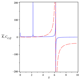
Figure 1: Graph of the extrinsic curvature $\bar{K}$ (solid blue curve) and the heat capacity $C_{J,Q}$ (dashed red curve) as a function of entropy, $S$, for an electric charge $Q=1$ and an angular momentum $J=1$.

III Extrinsic curvature of the phantom RN-AdS black hole

The action for the Einstein-Hilbert theory with phantom Maxwell field reads:

$$S=\int\sqrt{-g}\left(R+2\Lambda+2\eta F_{\mu\nu}F^{\mu\nu}\right)d^{4}x\ ,$$ (24)

where, $\Lambda$ is the cosmological constant, and $\eta=\pm 1$. RN-AdS black hole corresponds to $\eta=1$, while phantom couplings of the Maxwell field ( Phantom RN-AdS black hole) are obtained for $\eta=-1$. The metrics of these solutions, derived in ref25 , take the below form.

$$ds^{2}=f(r)dt^{2}-\frac{1}{f(r)}dr^{2}-r^{2}(d\theta^{2}+\sin^{2}\theta\,d\phi^{2})\ ,$$ (25)

where $f(r)$ is given by:

$$f(r)=1-\frac{2M}{r}-\frac{\Lambda}{3}r^{2}+\eta\frac{Q^{2}}{r^{2}}$$ (26)

The event horizon, $r_{+}$, of this solution can be determined by calculating the roots for the equation $f(r_{+})=0$. The mass of this black hole is expressed as a function of the thermodynamic variables.

$$M=\frac{1}{2}{{(S/\pi)}^{3/2}}(\frac{\pi}{S}-\frac{\Lambda}{3}+\frac{\eta{{\pi}^{2}}{{Q}^{2}}}{{{S}^{2}}})\$$ (27)

where $S=\pi r_{+}^{2}$ is the Bekenstein-Hawking entropy. According to the first law of thermodynamics, one can calculate the Hawking temperature, $T$, the electric potential, $\Phi$, and the specific heat capacity, $C_{Q}$, as follows:

$$T={(\frac{\partial M}{\partial S})}_{Q}=\frac{-\pi S+\Lambda{{S}^{2}}+\eta{{\pi}^{2}}{{Q}^{2}}}{-4{{(\pi S)}^{3/2}}}\$$ (28)

$$\Phi={(\frac{\partial M}{\partial Q})}_{S}=\frac{{{(S/\pi)}^{3/2}}\eta{{\pi}^{2}}Q}{{{S}^{2}}}\$$ (29)

$${{C}_{Q}}=T{{(\frac{\partial S}{\partial T})}_{Q}}=\frac{-2S(-\pi S+\Lambda{{S}^{2}}+\eta{{\pi}^{2}}{{Q}^{2}})}{(-\pi S-\Lambda{{S}^{2}}+3\eta{{\pi}^{2}}{{Q}^{2}})}$$ (30)

Using Eq. (5), it is easy to obtain the metric elements of the enthalpy potential in the coordinate $(S,\Phi)$. Then by applying Eqs. (7) and (8), the scalar curvature, $\overline{R}$, takes the following form:

$$\bar{R}=\frac{F(S,Q)}{(-S\pi+\Lambda{{S}^{2}}+{{\pi}^{2}}\eta{{Q}^{2}}){{(-S\pi-\Lambda{{S}^{2}}+3{{\pi}^{2}}\eta{{Q}^{2}})}^{2}}}$$ (31)

where,

$$F=-{\eta}^{2}{Q}^{4}{\pi}^{5}+\left(2\,\eta\,{Q}^{2}+10\,\Lambda\,{\eta}^{2}{Q}^{4}\right)S{\pi}^{4}+2\,{\Lambda}^{2}{S}^{4}\pi$$

$$+{S}^{2}\left(-9\,\eta\,{Q}^{2}\Lambda-1\right){\pi}^{3}+\left(3\,\Lambda-6\,{\Lambda}^{2}\eta\,{Q}^{2}\right){S}^{3}{\pi}^{2}$$ (32)

The first part of the denominator is zero only at $T=0$ and the roots of the second part of the curvature denominator gives us the phase transition points. Therefore, the curvature diverges exactly at these points where heat capacity diverges with no other additional roots. For the RN-AdS black hole, the scalar curvature (31) and the specific heat (30) are depicted in Figure 3 as a function of entropy and for a fixed value of electric charge $Q=0.25$. On the other hand, the extrinsic curvature opens an interesting and impressive avenue to the investigation of how phase transitions behave. In this case, we need to sit on a hypersurface with the normal vector ${{\overline{n}}_{Q}}=-1/\sqrt{\left|{{{\bar{g}}}^{QQ}}\right|}$ in which the extrinsic curvature associated with this hypersurface is given by:

$$\bar{K}=-{\frac{\left(\pi-2\,\Lambda\,S\right)\sqrt{\left|\eta\right|}\pi\,Q\sqrt{S}}{\left(-\pi\,S-\Lambda\,{S}^{2}+3\,\eta\,{\pi}^{2}{Q}^{2}\right)\sqrt{\left|-\pi\,S+\Lambda\,{S}^{2}+\eta\,{\pi}^{2}{Q}^{2}\right|}}}$$ (33)

The first term of the denominator shows the phase transition points, while the second is only zero at $T=0$. Interestingly, we see in Figure 3 that the extrinsic curvature has the same sign as heat capacity does, while in Figure 3, the scalar curvature does not have the same sign as the heat capacity around the phase transition points. In other words, extrinsic curvature reveals more information such as the stability/non-stability of heat capacities than the Ricci scalar does. Figure 4 indicates that the special Ricci tensor elements $\overline{R}_{SS}$ also exhibit a similar behavior around phase transition points such as heat capacity. Therefore, the extrinsic curvature $\overline{K}(S,Q)$ and the $\overline{R}_{SS}$ component of the Ricci tensor describe the phase transitions and the sign of the heat capacity, $C_{Q}$. Our work is a new method to identify stable regimes in the parameter space of black holes by studying the extrinsic curvature in their thermodynamic geometry.

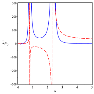
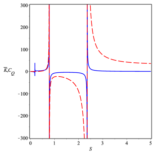
Figure 2: Graph of the scalar of curvature $\overline{R}$ (solid blue curve) and the heat capacity $C_{Q}$ (dashed red curve) as a function of entropy, $S$, in the RN-AdS case, for an electric charge $Q=0.25$ and a cosmological constant $\Lambda$=- 1.

Figure 3: Graph of the scalar of curvature $\overline{K}$ (solid blue curve) and the heat capacity $C_{Q}$ (dashed red curve) as a function of entropy, $S$, in the RN-AdS case, for an electric charge $Q=0.25$ and a cosmological constant $\Lambda$ =- 1.

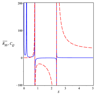
Figure 4: Graph of the scalar of curvature $\overline{R}_{SS}$ (solid blue curve) and the heat capacity $C_{Q}$ (dashed red curve) as a function of entropy, $S$, in the RN-AdS case, for an electric charge $Q=0.25$ and a cosmological constant $\Lambda$=- 1.

IV Ruppeiner curvature of RN black hole as an intrinsic curvature on a constant $J$ hypersurface

In article ref1 , the authors proposed a new measure of microscopic interactions and its effects on Ruppeiner curvature by considering a complete phase space of extensive variables. They obtained a new non-zero Ruppeiner curvature for RN black holes by setting $l\to\infty,\left({l=\frac{-3}{\Lambda}}\right)$, where $J\to 0$ limits in the scalar curvature for the Kerr-Newman-AdS (KN-AdS) black hole as follows:

$$\lim_{l\rightarrow\infty;J\rightarrow 0}{{R}_{KN-AdS}}=\frac{{{S}^{2}}+{{Q}^{2}}S+2{{Q}^{4}}}{{{\left(S+{{Q}^{2}}\right)}^{2}}\left({{Q}^{2}}-S\right)}$$ (34)

This non-vanishing scalar curvature is the result of another dimension specified by $J$ which fluctuates even if we set it to zero. It is surprising that this result is in contrast to a direct calculation on the Ruppeiner metric of the $RN$ which is zero ref23 . One of our objectives in this work is to explain the difference between these two results by applying the basic concepts of the extrinsic/ intrinsic geometry for a particular hypersurface (See Appx. B). In this framework, the Ruppeiner curvature of the KN-AdS black hole can be broken down into a purely intrinsic part, which yields a zero Ruppeiner curvature of the $RN$ black hole, and an extrinsic part, which measures the bending of the constant $J$ hypersurface; that is:

$${}^{(3)}{{R}_{KN-AdS}}={}^{(2)}R_{in}-({{K}^{2}}-{{K}_{ab}}{{K}^{ab}})-2{{(n_{;\beta}^{\alpha}{{n}^{\beta}}-{{n}^{\alpha}}n_{;\beta}^{\beta})}_{;\alpha}}$$ (35)

where, ${}^{(2)}R_{in}=R_{RN}=0$. Here the extrinsic part is expected to be exactly the same as Eq. (34). Now, let us investigate the accuracy of our claim about the KN-AdS black hole in the limits $l\to\infty$ and $J\to 0$.

The mass relation of the KN-AdS black hole ref26 as a function of thermodynamic variables can be written as:

$$M=[\frac{S}{4\pi}+\frac{\pi\left(4{{J}^{2}}+{{Q}^{2}}\right)}{4S}+\frac{{{Q}^{2}}}{2}+\frac{{{J}^{2}}}{{{l}^{2}}}$$ (36)

$$+\frac{S}{\pi{{l}^{2}}}\left({{Q}^{2}}+\frac{S}{\pi}+\frac{{{S}^{2}}}{2{{\pi}^{2}}{{l}^{2}}}\right)]^{\frac{1}{2}}$$

The Hawking temperature $T$ is also defined by:

$$T={{\left(\frac{\partial M}{\partial S}\right)}_{Q,J}}=\frac{{{S}^{2}}{{\pi}^{2}}{{l}^{4}}-4{{\pi}^{4}}{{l}^{4}}{{J}^{2}}-{{\pi}^{4}}{{l}^{4}}{{Q}^{2}}}{8{{\pi}^{3}}M{{S}^{2}}{{l}^{4}}}$$ (37)

$$+\frac{2{{S}^{2}}{{Q}^{2}}{{\pi}^{2}}{{l}^{2}}+4{{S}^{3}}\pi{{l}^{2}}+3{{S}^{4}}}{8{{\pi}^{3}}M{{S}^{2}}{{l}^{4}}}$$

It should be noted that, within the hypersurface framework, setting $J$ to zero is tantamount to living on the constant $J$ hypersurface ($J$- zero hapersurface) which has the following normal vector,

$${{n}_{J}}=-1/\sqrt{\left|{{{{g}}}^{JJ}}\right|}\,\,\ ;\,\,\ {{g}_{JJ}}=\frac{1}{T}\left(\frac{{{\partial}^{2}}M}{\partial{{J}^{2}}}\right).$$ (38)

Therefore, by making use of Eqs. (71) and (74), we have:

$$K^{2}=K_{\alpha\beta}K^{\alpha\beta}=0$$ (39)

On the other hand, the metric elements induced on the constant $J$ hypersurface can be given by:

$$g_{SS}=\lim_{l\rightarrow\infty;J\rightarrow 0}{\frac{1}{T}\left(\frac{{{\partial}^{2}}M}{\partial{{S}^{2}}}\right)}=\frac{3{{Q}^{2}}-S}{2S\left(S-{{Q}^{2}}\right)}$$ (40)

$$g_{SQ}=g_{QS}=\lim_{l\rightarrow\infty;J\rightarrow 0}{\frac{1}{T}\left(\frac{{{\partial}^{2}}M}{\partial S\partial Q}\right)}=\frac{-2Q}{S-{{Q}^{2}}}$$ (41)

$$g_{QQ}=\lim_{l\rightarrow\infty;J\rightarrow 0}{\frac{1}{T}\left(\frac{{{\partial}^{2}}M}{\partial{{Q}^{2}}}\right)}=\frac{4S}{S-{{Q}^{2}}}$$ (42)

The above elements are the same as those of the Ruppeiner metric for the $RN$ black hole ref23 . Therefore, the intrinsic curvature ${}^{(2)}R_{in}$ of the constant $J$ hypersurface equals the Ruppeiner curvature of the $RN$ black hole; i.e.,

$${}^{(2)}R_{in}=R_{RN}=0$$ (43)

Finally, based on Eq. (38), the last statement of Eq. (35) is given by:

$$\lim_{l\rightarrow\infty;J\rightarrow 0}{{{(n_{;\beta}^{\alpha}{{n}^{\beta}}-{{n}^{\alpha}}n_{;\beta}^{\beta})}_{;\alpha}}}=-\frac{\frac{{{S}^{2}}}{2}+\frac{{{Q}^{2}}S}{2}+{{Q}^{4}}}{{{\left(S+{{Q}^{2}}\right)}^{2}}\left({{Q}^{2}}-S\right)}$$ (44)

We can, therefore, conclude that the non-vanishing Ruppeiner curvature in the limits $J\to 0$ and $l\to\infty$ is extracted from the curvature of the KN-AdS black hole when one lives on the constant $J$ haypersurface. In addition, the Ruppeiner curvature of the RN black hole can be interpreted as the intrinsic curvature produced by the induced metric on the two dimensional hypersurface ($J$-zero hypersurface).

We may also check Eq. (73) for the Kerr black hole at $Q\to 0$ and $l\to\infty$ limits of the KN-AdS black hole to show that the intrinsic part of Eq. (73) is the Ruppeiner curvature of the Kerr black hole. Using the definition of the Ruppeiner metric for the complete phase space of the parameters (KN-AdS black hole), and assuming the limits $Q\to 0,\,\ l\to\infty$, we obtain the following equation for the Ricci scalar for a non- charged KN-AdS black hole.

$$\lim_{l\rightarrow\infty;Q\rightarrow 0}{{}^{(3)}{R}_{KN-AdS}}=\frac{\left(36{{J}^{2}}+{{S}^{2}}\right)S}{16{{J}^{4}}-{{S}^{4}}}$$ (45)

Also, the induced metric for the $Q$-zero hypersurface is calculated by:

$$g_{SS}=\lim_{l\rightarrow\infty;Q\rightarrow 0}{\frac{1}{T}\left(\frac{{{\partial}^{2}}M}{\partial{{S}^{2}}}\right)}={\frac{-24{J}^{2}{S}^{2}-48\,{J}^{4}+{S}^{4}}{2S\left(4\,{J}^{2}+{S}^{2}\right)\left(4\,{J}^{2}-{S}^{2}\right)}}$$ (46)

$$g_{SJ}=g_{JS}=\lim_{l\rightarrow\infty;Q\rightarrow 0}{\frac{1}{T}\left(\frac{{{\partial}^{2}}M}{\partial S\partial J}\right)}={\frac{4J\left(4\,{J}^{2}+3\,{S}^{2}\right)}{\left(4\,{J}^{2}+{S}^{2}\right)\left(4\,{J}^{2}-{S}^{2}\right)}}$$ (47)

$$g_{JJ}=\lim_{l\rightarrow\infty;Q\rightarrow 0}{\frac{1}{T}\left(\frac{{{\partial}^{2}}M}{\partial{{J}^{2}}}\right)}={\frac{-8{S}^{3}}{\left(4\,{J}^{2}+{S}^{2}\right)\left(4\,{J}^{2}-{S}^{2}\right)}}$$ (48)

One can obtain the following relation for the intrinsic curvature.

$$R_{in}=R_{kerr}={\frac{\left(12\,{J}^{2}+{S}^{2}\right)S}{16\,{J}^{4}-{S}^{4}}}$$ (49)

Moreover, for the $Q$-zero hypersurface with the normal vector,

$${{n}_{Q}}=-1/\sqrt{\left|{{{{g}}}^{QQ}}\right|}\,\,\ ;\,\,\ {{g}_{QQ}}=\frac{1}{T}\left(\frac{{{\partial}^{2}}M}{\partial{{Q}^{2}}}\right)$$ (50)

the extrinsic curvature is zero and $K^{2}=K_{\alpha\beta}K^{\alpha\beta}=0$. Now, we can successfully examine the validity of the following equation;

$$\lim_{l\rightarrow\infty;Q\rightarrow 0}{{R}_{KN-AdS}}={{}^{(2)}{R}_{Kerr}}-2\lim_{l\rightarrow\infty;Q\rightarrow 0}{{{(n_{;\beta}^{\alpha}{{n}^{\beta}}-{{n}^{\alpha}}n_{;\beta}^{\beta})}_{;\alpha}}}$$ (51)

where,

$$\lim_{l\rightarrow\infty;Q\rightarrow 0}{{{(n_{;\beta}^{\alpha}{{n}^{\beta}}-{{n}^{\alpha}}n_{;\beta}^{\beta})}_{;\alpha}}}=-12\,{\frac{S{J}^{2}}{16\,{J}^{4}-{S}^{4}}}$$ (52)

In summary, the Ruppeiner curvature of the Kerr black hole is similar to the intrinsic curvature produced by the induced metric on the two dimensional hypersurface ( i.e., constant $Q$ hypersurface). Our study indicates that in thermodynamic geometry, properties of the intrinsic and the extrinsic curvatures are important to obtain a complete geometric representation of thermodynamics in physical systems. The intrinsic curvature also help us to identify attractive, repulsive and non-interacting statistical interaction between the constituent parts of a thermodynamic system as we discuss in the next Section.

V Hypersurfaces and their intrinsic curvature in thermodynamic geometry of the Pauli paramagnetic gas

Thermodynamic curvature may explain the statistical interaction between particles in a thermodynamic system Ref1 ; Ref2 ; Ref3 . The thermodynamic curvature is positive for attractive interaction between particles, and negative for a repulsive interaction Ref3 . In case that particles have not any interaction with each other, the thermodynamic geometry is flat Ref1 . Now we consider thermodynamic geometry of a Pauli paramagnetic gas with indentical spin 1/2 fermions in the presence of an external magnetic field Ref4 . From the grand canonical distribution through the Fermi-Dirac statistics, the thermodynamic potential can be obtained as follows:

$$\phi(x,y,z)=Ix^{-{3\over 2}}[f_{5\over 2}(e^{-y-Jz})+f_{5\over 2}(e^{-y+Jz})].$$ (53)

where $I={{(2\pi m)^{3\over 2}}\over h^{3}}$ and $x=1/T,y=-\mu/T,z=-H/T$ are thermodynamic coordinates. $T$, $\mu$, and $H$ are also temperature, chemical potential, and external magnetic field, respectively. The $f_{n}(\eta)$ function is defined by:

$$f_{n}(\eta)={1\over\Gamma(n)}\int_{0}^{\infty}{{X^{n-1}dX}\over{e^{X}\over\eta}+1}$$ (54)

where $\eta=\exp({\mu\over{K_{B}T}})$ is called fugacity. The Ruppenier metric in thermodynamic geometry is given by:

$$g_{ij}={\partial^{2}\phi\over{\partial Y^{i}\partial Y^{j}}}\,\,\ ;\,\,\ Y^{i}=(x,y,z)$$ (55)

The Ricci scalar, ${}^{(3)}R$ was already obtained as a symmetric function of $z$ Ref4 . It means that the scalar curvature doesn’t depend on the orientation of external magnetic field. In the classical limit in the lack of the external magnetic field ($H\to 0$), when $\eta^{\pm}\rightarrow\eta$ and $f^{\pm}_{n}(\eta)\rightarrow\eta$; the ${}^{(3)}R$ is rewritten as follows:

$$\lim_{H\to 0(z\to 0)}{}^{(3)}R=-{9\over{2\rho}}$$ (56)

where in the classical regime, $\rho={2\over{\lambda^{3}}}\eta$ and $\lambda={h/(2\pi m_{0}K_{B}T)^{1\over 2}}$. Eq. (56) shows that in the classical limit, the curvature of a Pauli paramagnetic gas depends on the volume occupied by a single particle. The scalar curvature is also similar to the curvature that was obtained for a two-component ideal gas by Ruppeiner Ref5 .

In this letter we explore the physical properties of a Pauli paramagnetic gas by studying the intrinsic curvature of a hypersrface corresponding to a zero magnetic field ( $z\to 0$). The intrinsic curvature of $H$-zero hypersurface can be calculated as:

$${}^{(2)}R_{in}=-{5\over{2\rho}}$$ (57)

Because the intrinsic curvature is negative, so the statistical interactions of a Pauli paramagnetic gas can be repulsive which indicates a more stable paramagnetic gas. It should be noted that in the classical limit the extrinsic curvature vanish ($K=0$) and the Gauss-Codazzi relation is held in this case. On the other hand, the Ruppenier curvature for a non-interacting classical paramagnetic gas through Maxwell-Boltzman statistics with the thermodynamic potential, $\phi_{c}=4\pi Ix^{-{3\over 2}}e^{-y}{{\sinh(Jz)}\over{Jz}}$ ($J$ is magnetic momentum) Ref4 , takes the following form:

$${}^{(3)}R_{c}={\frac{{\lambda}^{3}Jz}{8\pi\,\eta\,\sinh\left(Jz\right)}}$$ (58)

From the equation of state ($PV=NK_{B}T$), one can see the curvature is proportional to the volume occupied by single particle (${}^{(3)}R_{c}=1/2\rho$) Ref4 . It is surprising that in the absence of an external magnetic field, the curvature is not zero (${}^{(3)}R_{c}={\frac{{\lambda}^{3}}{8\pi\,\eta}}$), while we would expect the curvature to be zero because of non-interaction particles Ref1 . To obtain a correct result we have to calculate the induced metric on a zero magnetic field hypersurface in the thermodynamic geometry. It can easily be shown that $H$-zero hypersurface is flat which indicates a non-interacting gas as expected. Our analysis indicates that the intrinsic geometry of hypersurfaces in thermodynamic geometry have important physical information. In order to have correct information we must study hypersurfaces in thermodynamic geometry.

VI conclusion

This work analyzed the thermodynamic geometry of a black hole from the perspective of an extrinsic curvature. It was found that the extrinsic scalar curvature represents the critical behavior of a second order phase transition in a thermodynamic system. Some particular Ricci tensor elements were found to have the same sign behavior as heat capacities. Another part of the article explained the relationship between the intrinsic, the extrinsic, and the total curvatures of thermodynamic geometry of a system by sitting on a certain hypersurface. For the KN-AdS black hole on a constant $J$ hypersurface, the curvature scalar was broken down into two parts. One was a zero intrinsic curvature (the Ruppeiner curvature of the RN black hole) while the other was an extrinsic part whose divergence points were the singularities of a non-rotating KN-AdS black hole. We also used the intrinsic curvature of the relevant hypersurface to investigate some thermodynamic properties such as stability and the statistical interaction.

As a result, the critical behavior of a thermodynamic system on an explicit hypersurface can be explained consistently by using intrinsic and extrinsic curvatures of this hypersurface.

Appendix A Partial derivative and bracket notation

When $f$, $g$, and $h$ are explicit functions of ($a,b$), we can obtain the following relation for the partial derivative.

$${{\left(\frac{\partial f}{\partial g}\right)}_{h}}=\frac{{{\left\{f,h\right\}}_{a,b}}}{{{\left\{g,h\right\}}_{a,b}}}$$ (59)

where,

$${{\{f,h\}}_{a,b}}={{\left(\frac{\partial f}{\partial a}\right)}_{b}}{{\left(\frac{\partial h}{\partial b}\right)}_{a}}-{{\left(\frac{\partial f}{\partial b}\right)}_{a}}{{\left(\frac{\partial h}{\partial a}\right)}_{b}}$$ (60)

Moreover, if one considers $a=a(c,d)$ and $b=b(c,d)$, Eq. (59) can be rewritten as:

$${{\left(\frac{\partial f}{\partial g}\right)}_{h}}=\frac{{{\left\{f,h\right\}}_{a,b}}}{{{\left\{g,h\right\}}_{a,b}}}=\frac{{{\left\{f,h\right\}}_{c,d}}}{{{\left\{g,h\right\}}_{c,d}}}$$ (61)

And, the determinant of the Jacobian transformation can be written in the bracket notation as in the form below:

$$det\left[\frac{\partial(f,g)}{\partial{(h,k)}}\right]=det\left(\begin{array}[]{cc}\vskip 6.0pt plus 2.0pt minus 2.0pt\cr{{\left(\frac{\partial f}{\partial h}\right)}_{k}}&{{\left(\frac{\partial f}{\partial k}\right)}_{h}}\\ \vskip 6.0pt plus 2.0pt minus 2.0pt\cr{{\left(\frac{\partial g}{\partial h}\right)}_{k}}&{{\left(\frac{\partial g}{\partial k}\right)}_{h}}\\ \end{array}\right)=\frac{{{\left\{f,g\right\}}_{a,b}}}{{{\left\{h,k\right\}}_{a,b}}}$$ (62)

Generally, the partial derivative for functions with $n+1$ variables can be calculated as follows:

$${{\left(\frac{\partial f}{\partial g}\right)}_{{{h}_{1}},.....,{{h}_{n}}}}=\frac{{{\left\{f,{{h}_{1}},...,{{h}_{n}}\right\}}_{{{q}_{1}},{{q}_{2}},...,{{q}_{n+1}}}}}{{{\left\{g,{{h}_{1}},...,{{h}_{n}}\right\}}_{{{q}_{1}},{{q}_{2}},...,{{q}_{n+1}}}}}$$ (63)

where, the $f$, $g$, and ${{h}_{n}}$ ($n=1,\,2,\,3,\,...$) are functions of ${{q}_{i}},i=1,...,n+1$ variables ref20 and,

$${{\left\{f,{{h}_{1}},...,{{h}_{n}}\right\}}_{{{q}_{1}},{{q}_{2}},...,{{q}_{n+1}}}}=$$ (64)

$$\sum\limits_{ijk....l=1}^{n+1}{{{\varepsilon}_{ijk...l}}\frac{\partial f}{\partial{{q}_{i}}}}\frac{\partial{{h}_{1}}}{\partial{{q}_{j}}}\frac{\partial{{h}_{2}}}{\partial{{q}_{k}}}...\frac{\partial{{h}_{n}}}{\partial{{q}_{l}}}$$

Appendix B The concepts of extrinsic and intrinsic curvatures for a hypersurface

In this section, we briefly review the concept of extrinsic curvature. For an n-dimensional manifold $\mathfrak{M}$, a special hypersurface $\Sigma$ can be defined as follows:

$$\Phi({{x}^{\alpha}})=0$$ (65)

where, ${{x}^{\alpha}}$s are the coordinates of the manifold $\mathfrak{M}$. The induced metric on $\Sigma$ can be written as:

$$ds_{\Sigma}^{2}={{g}_{\alpha\beta}}d{{x}^{\alpha}}d{{x}^{\beta}}={{g}_{\alpha\beta}}(\frac{\partial{{x}^{\alpha}}}{\partial{{y}^{a}}}d{{y}^{a}})(\frac{\partial{{x}^{\beta}}}{\partial{{y}^{b}}}d{{y}^{b}})={{h}_{ab}}d{{y}^{a}}d{{y}^{b}}$$ (66)

where,

$${{h}_{ab}}={{g}_{\alpha\beta}}E_{a}^{\alpha}E_{b}^{\beta};E_{a}^{\alpha}=\frac{\partial{{x}^{\alpha}}}{\partial{{y}^{a}}}$$ (67)

${{h}_{ab}}$ defines the induced metric on the hypersurface. A unit normal ${{n}_{\alpha}}$ can be introduced if ${{n}_{\alpha}}{{n}^{\alpha}}=\epsilon$ where $\varepsilon=1$ when $\Sigma$ is timelike and $\varepsilon=-1$ when $\Sigma$ is spacelike ref24 . We select that ${{n}^{\alpha}}$ points in the direction of increasing $\Phi$: ${{n}^{\alpha}}{{\Phi}_{,\alpha}}\rangle 0$. We can also easily show that:

$${{n}_{\alpha}}=\epsilon\frac{{{\Phi}_{,\alpha}}}{{{\left|{{g}^{\alpha\beta}}{{\Phi}_{,\alpha}}{{\Phi}_{,\beta}}\right|}^{\frac{1}{2}}}}$$ (68)

The inverse of the induced metric is obtained as follows:

$${{h}^{ab}}E_{a}^{\alpha}E_{b}^{\beta}={{g}^{\alpha\beta}}-\varepsilon{{n}^{\alpha}}{{n}^{\beta}}$$ (69)

One can also introduce the extrinsic curvature tensor on the hypersurface $\Sigma$ using the following relation:

$${{K}_{ab}}={{n}_{\alpha;\beta}}{E^{\alpha}}_{a}{E^{\beta}}_{b}=\frac{1}{2}{{L}_{n}}{{g}_{\alpha\beta}}{E^{\alpha}}_{a}{E^{\beta}}_{b}$$ (70)

where, the symbol ; and ${{L}_{n}}$ are the covariant and Lie derivatives of ${{g}_{\alpha\beta}}$ along ${{n}^{\alpha}}$, respectively. Therefore, the extrinsic curvature is defined by:

$$K={{h}^{ab}}{{K}_{ab}}=n_{;\alpha}^{\alpha}=\frac{1}{\sqrt{g}}{{\partial}_{\alpha}}\left(\sqrt{g}{{n}^{\alpha}}\right)$$ (71)

where, $g=det(g_{\alpha\beta})$. Suppose that a two-dimensional manifold is embedded in a three-dimensional space. The induced metric ${{h}_{ab}}$ and the extrinsic curvature ${{K}_{ab}}$ contain the necessary information about the properties of the hypersurface $\Sigma$. The full Riemann curvature tensor of the 3-dimensional space and the curvature tensor of the 2-dimensional hypersurface are related by the Gauss-Codazzi equation:

$${}^{(3)}{{R}_{\alpha\beta\gamma\sigma}}E_{a}^{\alpha}E_{b}^{\beta}E_{c}^{\gamma}E_{d}^{\sigma}={}^{(2)}{{R}_{abcd}}+\varepsilon({{K}_{ac}}{{K}_{bd}}-{{K}_{ad}}{{K}_{bc}})$$ (72)

This indicates that the three-dimensional Riemann tensor can be expressed in terms of the intrinsic and extrinsic curvature tensors of the hypersurface ref27 . Writing the Gauss-Codazzi equation in the contracted form, we obtain:

$${}^{(3)}R={}^{(2)}R_{in}+\epsilon({{K}^{2}}-{{K}_{ab}}{{K}^{ab}})+2\epsilon(n_{;\beta}^{\alpha}{{n}^{\beta}}-{{n}^{\alpha}}n_{;\beta}^{\beta})_{;\alpha}$$ (73)

This relation is the three-dimensional Ricci scalar evaluated on the hypersurface $\Sigma$. The ${}^{(2)}R$ is intrinsic Ricci scalar of the hypersurface. The third term, on the right hand side of the Equation, can be expressed as:

$${{K}_{ab}}{{K}^{ab}}=n_{;\beta}^{\alpha}n_{;\alpha}^{\beta}$$ (74)

For the two-dimensional space, the hypersurface $\Xi$ is a one-dimensional space with the normal vector ${{n}_{a}}=\left(1/\sqrt{\left|{{g}^{ab}}\right|}\right)\delta_{a}^{b}$. For this case, we have:

$${{K}^{2}}={{K}_{ab}}{{K}^{ab}}$$ (75)

Thus, the Ricci scalar ${}^{(2)}R$ is determined as follows:

$${}^{(2)}R=2\epsilon(n_{;b}^{a}{{n}^{b}}-{{n}^{a}}n_{;b}^{b})_{;a}$$ (76)

References

- (1) B. Mirza and M. Zamaninasab, Ruppeiner geometry of RN black holes: flat or curved?, JHEP 06 (2007) 059.
- (2) S. W. Hawking, Gravitational radiation from colliding black holes, Phys. Rev. Lett. 26, 1344 (1971).
- (3) J. D. Bekenstein, Black holes and entropy, Phys. Rev. D 7, 949, 2333 (1973).
- (4) J. M. Bardeen, B. Carter, and S. W. Hawking, The four laws of black hole mechanics, Commun. Math. Phys. 31, 161 (1973).
- (5) P. C. W. Davies, The Thermodynamic Theory of Black Holes, Proc. Roy. Soc. A 353, 499 (1977).
- (6) S. Hawking and D. N. Page, Thermodynamics of black holes in anti-de Sitter space, Commun. Math. Phys. 87, 577 (1983).
- (7) R. Banerjee, S. K. Modak, S. Samanta, Second order phase transition and thermodynamic geometry in Kerr-AdS black holes, Phys. Rev. D 84, 064024 (2011), [arXiv:1005.4832[hep-th]].
- (8) F. Weinhold, Metric geometry of equilibrium thermodynamics, J. Chem. Phys. 63, 2479 (1975).
- (9) G. Ruppeiner, Thermodynamics: A Riemannian geometric model, Phys. Rev. A 20, 1608 (1979).
- (10) G. Ruppeiner, Riemannian geometry in thermodynamic fluctuation theory, Rev. Mod. Phys. 67, 605 (1995) [Erratum-ibid. 68, 313 (1996)].
- (11) S. Ferara, G. Gibbons, and Kallosh, Black holes and critical points in moduli space, Nucl Phys. B 500 75, (1997).
- (12) J. Y. Shen, R. G. Cai, B. Wang and R. K. Su, Thermodynamic Geometry and Critical Behavior of Black Holes, Int. J. Mod. Phys. A 22, (2007) 11 [arXiv:gr-qc/0512035].
- (13) A. Medved, A commentary on Ruppeiner metrics for black holes, Mod. Phys. Lett. A. 23 2149, (2008).
- (14) S. Bellucci, B. N. Tiwari, Thermodynamic Geometry: Evolution, Correlation and Phase transition Physica A, 390 (2011) 2074 [arXiv:1010.5148v4 [gr-qc]].
- (15) A. Bravetti and F. Nettel, Thermodynamic curvature and ensemble nonequivalence, Phys. Rev. D 90, 044064 (2014).
- (16) Shao-Wen Wei, Yu-Xiao Liu, Yong-Qiang Wang, Heng Guo,Thermodynamic Geometry of black hole in the deformed Horava-Lifshitz gravity, EPL 99 20004 (2012) [arXiv:1002.1550v3 [hep-th]].
- (17) G. Ruppeiner, A. Sahay, T. Sarkar, G. Sengupta, Thermodynamic geometry, phase transitions, and the Widom line, Phys. Rev. E 2012, 86, 052103.
- (18) A. Bravetti, F. Nettel, Thermodynamic curvature and ensemble nonequivalence, Phys. Rev. D 2014, 90, 044064.
- (19) M. Azreg-Ainou, Geometrothermodynamics: Comments, critics, and supports, Eur. Phys. J. C 74, 2930 (2014) [arXiv:1311.6963v4 [gr-qc]].
- (20) S. A. Hoseeini Mansoori and Behrouz Mirza, Mohamadreza Fazel, Hessian matrix, specific heats, Nambu brackets, and thermodynamic geometry, JHEP 04 (2015) 115, [arXiv:1411.2582].
- (21) S. A. Hoseeini Mansoori and Behrouz Mirza, Correspondence of phase transition points and singularities of thermodynamic geometry of black holes, Eur. Phys. J. C 74, 2681 (2014) [arXiv:1308.1543].
- (22) J. E. Aman, I. Bengtsson, and N. Pidokrajt, Geometry of black hole thermodynamics, Gen. Rel. Grav.35, 1733 (2003) [arXiv:gr-qc/0304015].
- (23) J. E. Aman and N. Pidokrajt, Geometry of Higher-Dimensional Black Hole Thermodynamics, Phys. Rev. D 73 , 024017 (2006) [arXiv:hep-th/0510139].
- (24) D.F. Jardim, M.E. Rodrigues, S.J.M. Houndjo, Thermodynamics of the phantom Reissner-Nordstrom-AdS black hole, Eur. Phys. J. Plus 27 (2012). [arXiv:1202.2830v2 [gr-qc]].
- (25) M. M. Caldarelli, G. Cognola and D. Klemm, Thermodynamics of Kerr-Newmann-AdS black holes and conformal field theories, Class. and Quant. Grav. 17 (2000) 399 [hep-th/9908022].
- (26) D.L. Wiltshire, Spherically symmetric solutions of Einstein-Maxwell theory with a Gauss-Bonnet term, Phys. Lett. B. 169, 36 (1986)
- (27) J. D. Nulton and P. Salamon, Geometry of the ideal gas, Phys. Rev. A 31 2520 (1985).
- (28) H. Janyszek and R. Mrugal, Riemannian geometry and stability of thermodynamical equilibrium systems, J. Phys. A: Math. Gen. 23 477 (1990).
- (29) B. Mirza and H. Mohammadzadeh,Thermodynamic Geometry of Deformed Bosons and Fermions, J. Phys. A: Math. Theor. 44 475003 (2011).
- (30) K. Kaviani and A. Dalafi Rezaie, Pauli paramagnetic gas in the framework of Riemannian geometry, Phys. Rev. E 60, 3520 (1999).
- (31) G. Ruppeiner and C. Davis, Thermodynamic curvature of the multicomponent ideal gas, Phys. Rev. A 41 2200, (1990).
- (32) E. Poisson, A relativist’s toolkit, Cambridge University Press, The United Kingdom, (2004).