Boosting Information Spread:
An Algorithmic Approach

Abstract

The majority of influence maximization (IM) studies focus on targeting influential seeders to trigger substantial information spread in social networks. Motivated by the observation that incentives could “boost” users so that they are more likely to be influenced by friends, we consider a new and complementary $k$-boosting problem which aims at finding $k$ users to boost so to trigger a maximized “boosted” influence spread. The $k$-boosting problem is different from the IM problem because boosted users behave differently from seeders: boosted users are initially uninfluenced and we only increase their probability to be influenced. Our work also complements the IM studies because we focus on triggering larger influence spread on the basis of given seeders. Both the NP-hardness of the problem and the non-submodularity of the objective function pose challenges to the $k$-boosting problem. To tackle the problem on general graphs, we devise two efficient algorithms with the data-dependent approximation ratio. To tackle the problem on bidirected trees, we present an efficient greedy algorithm and a dynamic programming that is a fully polynomial-time approximation scheme. Extensive experiments using real social networks and synthetic bidirected trees verify the efficiency and effectiveness of the proposed algorithms. In particular, on general graphs, we show that boosting solutions returned by our algorithms achieves boosts of influence that are up to several times higher than those achieved by boosting intuitive solutions with no approximation guarantee. We also explore the “budget allocation” problem experimentally, demonstrating the beneficial of allocating the budget to both seeders and boosted users.

I Introduction

With the popularity of online social networks, viral marketing, which is a marketing strategy to exploit online word-of-mouth effects, has become a powerful tool for companies to promote sales. In viral marketing campaigns, companies target influential users by offering free products or services with the hope of triggering a chain reaction of product adoption. Initial adopters or seeds are often used interchangeably to refer to these targeted users. Motivated by the need for effective viral marketing strategies, influence maximization has become a fundamental research problem in the past decade. The goal of influence maximization is usually to identify influential initial adopters [1, 2, 3, 4, 5, 6, 7, 8].

In practical marketing campaigns, companies often consider a mixture of multiple promotion strategies. Targeting influential users as initial adopters is one tactic, and we list some others as follows.

• Customer incentive programs: Companies offer incentives such as coupons or product trials to attract potential customers. Targeted customers are in general more likely to be influenced by their friends.

• Social media advertising: Companies reach intended audiences via digital advertising. According to an advertising survey [9], owned online channels such as brand-managed sites are the second most trusted advertising formats, second only to recommendations from family and friends. We believe that customers targeted by advertisements are more likely to follow their friends’ purchases.

• Referral marketing: Companies encourage customers to refer others to use the product by offering rewards such as cash back. In this case, targeted customers are more likely to influence their friends.

As one can see, these marketing strategies are able to “boost” the influence transferring through customers. Furthermore, for companies, the cost of “boosting” a customer (e.g., the average redemption and distribution cost per coupon, or the advertising cost per customer) is much lower than the cost of nurturing an influential user as an initial adopter and a product evangelist. Although identifying influential initial adopters have been actively studied, very little attention has been devoted to studying how to utilize incentive programs or other strategies to further increase the influence spread of initial adopters.

In this paper, we study the problem of finding $k$ boosted users so that when their friends adopt a product, they are more likely to make the purchase and continue to influence others. Motivated by the need for modeling boosted customers, we propose a novel influence boosting model. In our model, seed users generate influence same as in the classical Independent Cascade (IC) model. In addition, we introduce the boosted user as a new type of user. They represent customers with incentives such as coupons. Boosted users are uninfluenced at the beginning of the influence propagation process, However, they are more likely to be influenced by their friends and further spread the influence to others. In other words, they “boost” the influence transferring through them. Under the influence boosting model, we study how to boost the influence spread given initial adopters. More precisely, given initial adopters, we are interested in identifying $k$ users among other users, so that the expected influence spread upon “boosting” them is maximized. Because of the essential differences in behaviors between seed users and boosted users, our work is very different from influence maximization studies focusing on selecting seeds.

Our work also complements the studies of influence maximization problems. First, compared with nurturing an initial adopter, boosting a potential customer usually incurs a lower cost. For example, companies may need to offer free products to initial adopters, but only need to offer coupons to boost potential customers. With both our methods that identify users to boost and influence maximization algorithms that select initial adopters, companies have more flexibility in allocating their marketing budgets. Second, initial adopters are sometimes predetermined. For example, they may be advocates of a particular brand or prominent bloggers in the area. In this case, our study suggests how to effectively utilize incentive programs or similar marketing strategies to take the influence spread to the next level.

Contributions. We study a novel problem of how to boost the influence spread when the initial adopters are given. We summarize our contributions as follows.

• We present the influence boosting model, which integrates the idea of boosting into the Independent Cascade model. We formulate a $k$-boosting problem that asks how to maximize the boost of influence spread under the influence boosting model. The $k$-boosting problem is NP-hard. Computing the boost of influence spread is #P-hard. Moreover, the boost of influence spread does not possess the submodularity, meaning that the greedy algorithm does not provide performance guarantee.

• We present approximation algorithms PRR-Boost and PRR-Boost-LB for the $k$-boosting problem. For the $k$-boosting problem on bidirected trees, we present a greedy algorithm Greedy-Boost based on a linear-time exact computation of the boost of influence spread and a fully polynomial-time approximation scheme (FPTAS) DP-Boost that returns near-optimal solutions.  DP-Boost provides a benchmark for the greedy algorithm, at least on bi-directed trees, since it is very hard to find near optimal solutions in general cases. Moreover, the algorithms on bidirected trees may be applicable to situations where information cascades more or less follow a fixed tree architecture.

• We conduct extensive experiments using real social networks and synthetic bidirected trees. Experimental results show the efficiency and effectiveness of our proposed algorithms, and their superiority over intuitive baselines.

Paper organization. Section II provides background. We describe the influence boosting model and the $k$-boosting problem in Section III. We present building blocks of PRR-Boost and PRR-Boost-LB for the $k$-boosting problem in Section IV, and the detailed algorithm design in Section V. We present Greedy-Boost and DP-Boost for the $k$-boosting problem on bidirected trees in Section VI. We show experimental results in Sections VII-VIII. Section IX concludes the paper.

II Background and related work

In this section, we provide backgrounds about influence maximization problems and related works.

Classical influence maximization problems. Kempe et al. [1] first formulated the influence maximization problem that asks to select a set $S$ of $k$ nodes so that the expected influence spread is maximized under a predetermined influence propagation model. The Independent Cascade (IC) model is one classical model that describes the influence diffusion process [1]. Under the IC model, given a graph $G=(V,E)$, influence probabilities on edges and a set $S\subseteq V$ of seeds, the influence propagates as follows. Initially, nodes in $S$ are activated. Each newly activated node $u$ influences its neighbor $v$ with probability $p_{uv}$. The influence spread of $S$ is the expected number of nodes activated at the end of the influence diffusion process. Under the IC model, the influence maximization problem is NP-hard [1] and computing the expected influence spread for a given $S$ is #P-hard [4]. A series of studies have been done to approximate the influence maximization problem under the IC model or other diffusion models [10, 3, 4, 11, 12, 6, 7, 8, 13].

Influence maximization on trees. Under the IC model, tree structure makes the influence computation tractable. To devise greedy “seed-selection” algorithms on trees, several studies presented various methods to compute the “marginal gain” of influence spread on trees [4, 14]. Our computation of “marginal gain of boosts” on trees is more advanced than the previous methods: It runs in linear-time, it considers the behavior of “boosting”, and we assume that the benefits of “boosting” can be transmitted in both directions of an edge. On bidirected trees, Bharathi et al. [15] described an FPTAS for the classical influence maximization problem. Our FPTAS on bidirected trees is different from theirs because “boosting” a node and targeting a node as a “seed” have significantly different effects.

Boost the influence spread. Several works studied how to recommend friends or inject links into social networks in order to boost the influence spread [16, 17, 18, 19, 20, 21]. Lu et al. [22] studied how to maximize the expected number of adoptions by targeting initial adopters of a complementing product. Chen et al. [23] considered the amphibious influence maximization. They studied how to select a subset of seed content providers and a subset of seed customers so that the expected number of influenced customers is maximized. Their model differs from ours in that they only consider influence originators selected from content providers, which are separated from the social network, and influence boost is only from content providers to consumers in the social network. Yang et al. [21] studied how to offer discounts assuming that the probability of a customer being an initial adopter is a known function of the discounts offered to him. They studied how to offer discounts to customers so that the influence cascades triggered is maximized. Different from the above studies, we study how to boost the spread of influence when seeds are given. We assume that we can give incentives to some users (i.e., “boost” some users) so that they are more likely to be influenced by their friends, but they themselves would not become adopters without friend influence. This article is an extended version of our conference paper [24] that formulated the $k$-boosting problem and presented algorithms for it. We add two new algorithms that tackle the $k$-boosting problem in bidirected trees, and report new experimental results.

III Model and Problem Definition

In this section, we first define the influence boosting model and the $k$-boosting problem. Then, we highlight the challenges associated with solving the proposed problem.

III-A Model and Problem Definition

Traditional studies of the influence maximization problem focus on how to identify a set of $k$ influential users (or seeds) who can trigger the largest influence diffusion. In this paper, we aim to boost the influence propagation assuming that seeds are given. We first define the influence boosting model.

Definition 1 (Influence Boosting Model).

Suppose we are given a directed graph $G\!=\!(V,E)$ with $n$ nodes and $m$ edges, two influence probabilities $p_{uv}$ and $p^{\prime}_{uv}$ (with $p^{\prime}_{uv}>p_{uv}$) on each edge $e_{uv}$, a set $S\subseteq V$ of seeds, and a set $B\subseteq V$ of boosted nodes. Influence propagates in discrete time steps as follows. If $v$ is not boosted, each of its newly-activated in-neighbor $u$ influences $v$ with probability $p_{uv}$. If $v$ is a boosted node, each of its newly-activated in-neighbor $u$ influences $v$ with probability $p^{\prime}_{uv}$.

In Definition 1, we assume that “boosted” users are more likely to be influenced. Our study can also be adapted to the case where boosted users are more influential: if a newly-activated user $u$ is boosted, she influences her neighbor $v$ with probability $p^{\prime}_{uv}$ instead of $p_{uv}$. To simplify the presentation, we focus on the influence boosting model in Definition 1.

$\boldsymbol{B}$	$\boldsymbol{\sigma_{S}(B)}$	$\boldsymbol{\Delta_{S}(B)}$
$\emptyset$	1.22	0.00
$\{v_{0}\}$	1.44	0.22
$\{v_{1}\}$	1.24	0.02
$\{v_{0},v_{1}\}$	1.48	0.26

Figure 1: Example of the influence boosting model ($S\!=\!\{s\}$).

Let $\sigma_{S}(B)$ be the expected influence spread of $S$ upon boosting nodes in $B$. We refer to $\sigma_{S}(B)$ as the boosted influence spread. Let $\Delta_{S}(B)=\sigma_{S}(B)-\sigma_{S}(\emptyset)$. We refer to $\Delta_{S}(B)$ as the boost of influence spread of $B$, or simply the boost of $B$. Consider the example in Figure 1. We have $\sigma_{S}(\emptyset)=1.22$, which is essentially the influence spread of $S$ in the IC model. When we boost node $v_{0}$, we have $\sigma_{S}(\{v_{0}\})=1+0.4+0.04=1.44$, and $\Delta_{S}(\{v_{0}\})=0.22$. We now formulate the $k$-boosting problem.

Definition 2 ($k$-Boosting Problem).

Given a directed graph $G=(V,E)$, influence probabilities $p_{uv}$ and $p^{\prime}_{uv}$ on every edges $e_{uv}$, and a set $S\subseteq V$ of seed nodes, find a boost set $B\subseteq V$ with $k$ nodes, such that the boost of influence spread of $B$ is maximized. That is, determine $B^{*}\subseteq V$ such that

$$B^{*}=\operatorname{arg\,max}_{B\subseteq V,|B|\leq k}\Delta_{S}(B).$$ (1)

By definition, the $k$-boosting problem is very different from the classical influence maximization problem. In addition, boosting nodes that significantly increase the influence spread when used as additional seeds could be extremely inefficient. For example, consider the example in Figure 1, if we are allowed to select one more seed, we should select $v_{1}$. However, if we can boost a node, boosting $v_{0}$ is much better than boosting $v_{1}$. Section VII provides more experimental results.

III-B Challenges of the Boosting Problem

We now provide key properties of the $k$-boosting problem and show the challenges we face. Theorem 1 summarizes the hardness of the $k$-boosting problem.

Theorem 1 (Hardness).

The $k$-boosting problem is NP-hard. Computing $\Delta_{S}(B)$ given $S$ and $B$ is #P-hard.

Proof.

The NP-hardness is proved by a reduction from the NP-complete Set Cover problem [25]. The #P-hardness of the computation is proved by a reduction from the #P-complete counting problem of $s$-$t$ connectedness in directed graphs [26]. The full analysis can be found in the appendix. ∎

Non-submodularity of the boost of influence. Because of the above hardness results, we explore approximation algorithms to tackle the $k$-boosting problem. In most influence maximization problems, the expected influence of the seed set $S$ (i.e., the objective function) is a monotone and submodular function of $S$. Thus, a natural greedy algorithm returns a solution with an approximation guarantee [1, 6, 7, 8, 13, 28]. However, the objective function $\Delta_{S}(B)$ in our problem is neither submodular nor supermodular on the set $B$ of boosted nodes. On one hand, when we boost several nodes on different parallel paths from seed nodes, their overall boosting effect exhibits a submodular behavior. On the other hand, when we boost several nodes on a path starting from a seed node, their boosting effects can be cumulated along the path, generating a larger overall effect than the sum of their individual boosting effect. This is in fact a supermodular behavior. To illustrate, consider the graph in Figure 1, we have $\Delta_{S}(\{v_{0},v_{1}\})-\Delta_{S}(\{v_{0}\})=0.04$, which is larger than $\Delta_{S}(\{v_{1}\})-\Delta_{S}(\emptyset)=0.02$. In general, the boosted influence has a complicated interaction between supermodular and submodular behaviors when the boost set grows, and is neither supermodular nor submodular. The non-submodularity of $\Delta_{S}(\cdot)$ indicates that the boosting set returned by the greedy algorithm may not have the $(1-1/e)$-approximation guarantee. Therefore, the non-submodularity of the objective function poses an additional challenge.

IV Boosting on General Graphs: Building Blocks

In this section, we present three building blocks for solving the $k$-boosting problem: (1) a state-of-the-art influence maximization framework, (2) the Potentially Reverse Reachable Graph for estimating the boost of influence spread, and (3) the Sandwich Approximation strategy [22] for maximizing non-submodular functions. Our algorithms PRR-Boost and PRR-Boost-LB integrate the three building blocks. We will present their detailed algorithm design in the next section.

IV-A State-of-the-art influence maximization techniques

One state-of-the-art influence maximization framework is the Influence Maximization via Martingale (IMM) method [8] based on the idea of Reverse-Reachable Sets (RR-sets) [6]. We utilize the IMM method in this work, but other similar frameworks based on RR-sets (e.g., SSA/D-SSA [13]) could also be applied.

RR-sets. An RR-set for a node $r$ is a random set $R$ of nodes, such that for any seed set $S$, the probability that $R\cap S\neq\emptyset$ equals the probability that $r$ can be activated by $S$ in a random diffusion process. Node $r$ may also be selected uniformly at random from $V$, and the RR-set will be generated accordingly with $r$. One key property of RR-sets is that the expected influence of $S$ equals to $n\cdot\mathbb{E}[\mathbb{I}({R\cap S\neq\emptyset})]$ for all $S\subseteq V$, where $\mathbb{I}({\cdot})$ is the indicator function and the expectation is taken over the randomness of $R$.

General IMM algorithm. The IMM algorithm has two phases. The sampling phase generates a sufficiently large number of random RR-sets such that the estimation of the influence spread is “accurate enough”. The node selection phase greedily selects $k$ seed nodes based on their estimated influence spread. If generating a random RR-set takes time $O(EPT)$, IMM returns a $(1-1/e-\epsilon)$-approximate solution with probability at least $1-n^{-\ell}$, and runs in $O(\frac{EPT}{OPT}\cdot(k+\ell)(n+m)\log n/\epsilon^{2})$ expected time, where $OPT$ is the optimal expected influence.

IV-B Potentially Reverse Reachable Graphs

We now describe how we estimate the boost of influence. The estimation is based on the concept of the Potentially Reverse Reachable Graph (PRR-graph) defined as follows.

Definition 3 (Potentially Reverse Reachable Graph).

Let $r$ be a node in $G$. A Potentially Reverse Reachable Graph (PRR-graph) $R$ for a node $r$ is a random graph generated as follows. We first sample a deterministic copy $g$ of $G$. In the deterministic graph $g$, each edge $e_{uv}$ in graph $G$ is “live” in $g$ with probability $p_{uv}$, “live-upon-boost” with probability $p^{\prime}_{uv}-p_{uv}$, and “blocked” with probability $1-p^{\prime}_{uv}$. The PRR-graph $R$ is the minimum subgraph of $g$ containing all paths from seed nodes to $r$ through non-blocked edges in $g$. We refer to $r$ as the “root node”. When $r$ is also selected from $V$ uniformly at random, we simply refer to the generated PRR-graph as a random PRR-graph (for a random root).

Figure 2: Example of a Potentially Reverse Reachable Graph.

Figure 2 shows an example of a PRR-graph $R$. The directed graph $G$ contains $12$ nodes and $16$ edges. Node $r$ is the root node. Shaded nodes are seed nodes. Solid, dashed and dotted arrows with crosses represent live, live-upon-boost and blocked edges, respectively. The PRR-graph for $r$ is the subgraph in the dashed box. It contains $9$ nodes and $13$ edges. Nodes and edges outside the dashed box do not belong to the PRR-graph, because they are not on any paths from seed nodes to $r$ that only contain non-blocked edges. By definition, a PRR-graph may contain loops. For example, the PRR-graph in Figure 2 contains a loop among nodes $v_{1}$, $v_{5}$, and $v_{2}$.

Estimating the boost of influence. Let $R$ be a given PRR-graph with root $r$. By definition, every edge in $R$ is either live or live-upon-boost. Given a path in $R$, we say that it is live if and only if it contains only live edges. Given a path in $R$ and a set of boosted nodes $B\subseteq V$, we say that the path is live upon boosting $B$ if and only if the path is not a live one, but every edge $e_{uv}$ on it is either live or live-upon-boost with $v\!\in\!B$. For example, in Figure 2, the path from $v_{3}$ to $r$ is live, and the path from $v_{7}$ to $r$ via $v_{4}$ and $v_{1}$ is live upon boosting $\{v_{1}\}$. Define $f_{R}(B):2^{V}\!\rightarrow\!\{0,1\}$ as: $f_{R}(B)=1$ if and only if, in $R$, (1) there is no live path from seed nodes to $r$; and (2) a path from a seed node to $r$ is live upon boosting $B$. Intuitively, in the deterministic graph $R$, $f_{R}(B)=1$ if and only if the root node is inactive without boosting, and active upon boosting nodes in $B$. In Figure 2, if $B=\emptyset$, there is no live path from the seed node $v_{7}$ to $r$ upon boosting $B$. Therefore, we have $f_{R}(\emptyset)=0$. Suppose we boost a single node $v_{1}$. There is a live path from the seed node $v_{7}$ to $r$ that is live upon boosting $\{v_{1}\}$, and thus we have $f_{R}(\{v_{1}\})=1$. Similarly, we have $f_{R}(\{v_{3}\})=f_{R}(\{v_{2},v_{5}\})=1$. Based on the above definition of $f_{R}(\cdot)$, we have the following lemma.

Lemma 1.

For any $B\subseteq V$, we have $n\cdot\mathbb{E}[f_{R}(B)]=\Delta_{S}(B)$, where the expectation is taken over the randomness of $R$.

Proof.

For a random PRR-graph $R$ whose root node is randomly selected, $\Pr[f_{R}(B)=1]$ equals the difference between probabilities that a random node in $G$ is activated given that we boost $B$ and $\emptyset$. ∎

Let $\mathcal{R}$ be a set of independent random PRR-graphs, define

$$\hat{\Delta}_{\mathcal{R}}(B)=\frac{n}{|\mathcal{R}|}\cdot\sum_{R\in\mathcal{R}}f_{R}(B),\forall B\subseteq V.$$ (2)

By Chernoff bound, $\hat{\Delta}_{\mathcal{R}}(B)$ closely estimates $\Delta_{S}(B)$ for any $B\subseteq V$ if $|\mathcal{R}|$ is sufficiently large.

IV-C Sandwich Approximation Strategy

To tackle the non-submodularity of function $\Delta_{S}(\cdot)$, we apply the Sandwich Approximation (SA) strategy [22]. First, we find submodular lower and upper bound functions of $\Delta_{S}$, denoted by $\mu$ and $\nu$. Then, we select node sets $B_{\Delta}$, $B_{\mu}$ and $B_{\nu}$ by greedily maximizing $\Delta_{S}$, $\mu$ and $\nu$ under the cardinality constraint of $k$. Ideally, we return $B_{\text{sa}}=\operatorname{arg\,max}_{B\in\{B_{\mu},B_{\nu},B_{\Delta}\}}\Delta_{S}(B)$ as the final solution. Let the optimal solution of the $k$-boosting problem be $B^{*}$ and let $OPT=\Delta_{S}(B^{*})$. Suppose $B_{\mu}$ and $B_{\nu}$ are $(1-1/e-\epsilon)$-approximate solutions for maximizing $\mu$ and $\nu$, we have

$$\Delta_{S}(B_{\text{sa}}) \geq\frac{\mu(B^{*})}{\Delta_{S}(B^{*})}\cdot(1-1/e-\epsilon)\cdot OPT,$$ (3)

$$\Delta_{S}(B_{\text{sa}}) \geq\frac{\Delta_{S}(B_{\nu})}{\nu(B_{\nu})}\cdot(1-1/e-\epsilon)\cdot OPT.$$ (4)

Thus, to obtain a good approximation guarantee, at least one of $\mu$ and $\nu$ should be close to $\Delta_{S}$. In this work, we derive a submodular lower bound $\mu$ of $\Delta_{S}$ using the definition of PRR-graphs. Because $\mu$ is significantly closer to $\Delta_{S}$ than any submodular upper bound we have tested, we only use the lower bound function $\mu$ and the “lower-bound side” of the SA strategy with approximation guarantee in Equation 3.

Submodular lower bound. We now derive a submodular lower bound of $\Delta_{S}$. Let $R$ be a PRR-graph with the root node $r$. Let $C_{R}=\{v|f_{R}(\{v\})=1\}$. We refer to nodes in $C_{R}$ as critical nodes of $R$. Intuitively, the root node $r$ becomes activated if we boost any node in $C_{R}$. For any node set $B\subseteq V$, define $f_{R}^{-}(B)=\mathbb{I}({B\cap C_{R}\neq\emptyset})$. By definition of $C_{R}$ and $f_{R}^{-}(\cdot)$, we have $f^{-}_{R}(B)\leq f_{R}(B)$ for all $B\subseteq V$. Moreover, because the value of $f_{R}^{-}(B)$ is based on whether the node set $B$ intersects with a fixed set $C_{R}$, $f^{-}_{R}(B)$ is a submodular function on $B$. For any $B\subseteq V$, define $\mu(B)=n\cdot\mathbb{E}[f^{-}_{R}(B)]$ where the expectation is taken over the randomness of $R$. Lemma 2 shows the properties of the function $\mu$.

Lemma 2.

We have $\mu(B)\leq\Delta_{S}(B)$ for all $B\subseteq V$. Moreover, $\mu(B)$ is a submodular function of $B$.

Proof.

For all $B\subseteq V$, we have $\mu(B)\leq\Delta_{S}(B)$ because we have $f^{-}_{R}(B)\leq f_{R}(B)$ for any PRR-graph $R$. Moreover, $\mu(B)$ is submodular on $B$ because $f^{-}_{R}(B)$ is submodular on $B$ for any PRR-graph $R$. ∎

Our experiments show that $\mu$ is close to $\Delta_{S}$ especially for small $k$ (e.g., less than a thousand). Define

$$\hat{\mu}_{\mathcal{R}}(B)=\frac{n}{|\mathcal{R}|}\cdot\sum_{R\in\mathcal{R}}f^{-}_{R}(B),\forall B\subseteq V.$$

Because $f_{R}^{-}(B)$ is submodular on $B$ for any PRR-graph $R$, $\hat{\mu}_{\mathcal{R}}(B)$ is submodular on $B$. Moreover, by Chernoff bound, $\hat{\mu}_{\mathcal{R}}(B)$ is close to $\mu(B)$ when $|\mathcal{R}|$ is sufficiently large.

Remarks on the lower bound function $\mu(B)$. The lower bound function $\mu(B)$ does correspond to a physical diffusion model, as we now explain. Roughly speaking, $\mu(B)$ is the influence spread in a diffusion model with the boost set $B$, and the constraint that at most one edge on the influence path from a seed node to an activated node can be boosted. More precisely, on every edge $e_{uv}$ with $v\in B$, there are three possible outcomes when $u$ tries to activate $v$: (a) normal activation: $u$ successfully activates $v$ without relying on the boost of $v$ (with probability $p_{uv}$), (b) activation by boosting: $u$ successfully activates $v$ but relying on the boost of $v$ (with probability $p^{\prime}_{uv}-p_{uv}$); and (c) no activation: $u$ fails to activate $v$ (with probability $1-p^{\prime}_{uv}$). In the diffusion model, each activated node records whether it is normally activated or activated by boosting. Initially, all seed nodes are normally activated. If a node $u$ is activated by boosting, we disallow $u$ to activate its out-neighbors by boosting. Moreover, when $u$ normally activates $v$, $v$ inherits the status from $u$ and records its status as activated by boosting. However, if later $u$ can be activated again by another in-neighbor normally, $u$ can resume the status of being normally activated, resume trying to activate its out-neighbors by boosting. Furthermore, this status change recursively propagates to $u$’s out-neighbors that were normally activated by $u$ and inherited the “activated-by-boosting” status from $u$, so that they now have the status of “normally-activated” and can activate their out-neighbors by boosting. All the above mechanisms are to insure that the chain of activation from any seed to any activated node uses at most one activation by boosting.

Admittedly, the above model is convoluted, while the PRR-graph description of $\mu(B)$ is more direct and is easier to analyze. Indeed, we derived the lower bound function $\mu(B)$ directly from the concept of PRR-graphs first, and then “reverse-engineered” the above model from the PRR-graph model. Our insight is that by fixing the randomness in the original influence diffusion model, it may be easier to derive submodular lower-bound or upper-bound functions. Nevertheless, we believe the above model also provides some intuitive understanding of the lower bound model — it is precisely submodular because it disallows multiple activations by boosting in any chain of activation sequences.

V Boosting On General Graphs: Algorithm Design

In this section, we first present how we generate random PRR-graphs. Then we obtain overall algorithms by integrating the general IMM algorithm with PRR-graphs and the Sandwich Approximation strategy.

V-A Generating PRR-graphs

We classify PRR-graphs into three categories. Let $R$ be a PRR-graph with root node $r$. (1) Activated: If there is a live path from a seed node to $r$; (2) Hopeless: There is no path from seeds to $r$ with at most $k$ non-live edges; (3) “Boostable”: not the above two categories. If $R$ is not boostable (i.e. case (1) or (2)), we have $f_{R}(B)=f_{R}^{-}(B)=0$ for all $B\subseteq V$. Therefore, for “non-boostable” PRR-graphs, we only count their occurrences and we terminate the generation of them once we know they are not boostable. Algorithm 1 depicts generation of a random PRR-graph in two phases. The first phase (Algorithms 1-1) generates a PRR-graph $R$. If $R$ is boostable, the second phase compresses $R$ to reduce its size. Figure 3 shows the results of two phases, given that the status sampled for every edge is same as that in Figure 2.

(a) Results of phase I

(b) Results of phase II

Figure 3: Generation of a PRR-Graph. (Solid and dashed arrows represent live and live-upon-boost edges respectively.)

1

2Select a random node $r$ as the root node

3 if $r\in S$ then return $R$ is activated

4 Create a graph $R$ with a singleton node $r$

5 Create a double-ended queue $Q$ with $(r,0)$

6 Initialize $d_{r}[r]\leftarrow 0$ and $d_{r}[v]\leftarrow+\infty,\forall v\neq r$

7 while $Q$ is not empty do

8       $(u,d_{ur})\leftarrow Q$.dequeue_front()

9       if $d_{ur}>d_{r}[u]$ then continue

10        // we’ve processed $u$ for each non-blocked incoming edge $e_{vu}$ of $u$ do

11             $d_{vr}\leftarrow\mathbb{I}({e_{vu}\text{ is {live-upon-boost}}})+d_{ur}$

12             if $d_{vr}>k$ then continue

13              // pruning Add $e_{vu}$ to $R$

14             if $d_{vr}<d_{r}[v]$ then

15                   $d_{r}[v]\leftarrow d_{vr}$

16                   if $v\in S$ then

17                         if $d_{r}[v]=0$ then return $R$ is activated

18                        

19                  else if $d_{vr}\!=\!d_{ur}$ then $Q$.enqueue_front($(v,d_{vr})$)

20                   else $Q$.enqueue_back($(v,d_{vr})$)

21                  

22            

23      

24if there is no seed in $R$ then return $R$ is hopeless

25 Compress the boostable $R$ to reduce its size

return a compressed boostable $R$

Algorithm 1 Generating a random PRR-graph $(G,S,k)$

Phase I: Generating a PRR-graph. Let $r$ be a random node. We include into $R$ all non-blocked paths from seed nodes to $r$ with at most $k$ live-upon-boost edges via a a backward Breadth-First Search (BFS) from $r$. The status of each edge (i.e., live, live-upon-boost, blocked) is sampled when we first process it. The detailed backward BFS is as follows. Define the distance of a path from $u$ to $v$ as the number of live-upon-boost edges on it. Then, the shortest distance from $v$ to $r$ is the minimum number of nodes we have to boost so that at least a path from $v$ to $r$ becomes live. For example, in Figure 3a, the shortest distance from $v_{7}$ to $r$ is one. We use $d_{r}[\cdot]$ to maintain the shortest distances from nodes to the root node $r$. Initially, we have $d_{r}[r]=0$ and we enqueue $(r,0)$ into a double-ended queue $Q$. We repeatedly dequeue and process a node-distance pair $(u,d_{ur})$ from the head of $Q$, until the queue is empty. Note that the distance $d_{ur}$ in a pair $(u,d_{ur})$ is the shortest known distance from $u$ to $r$ when the pair was enqueued. Thus we may find $d_{ur}>d_{r}[u]$ in Algorithm 1. Pairs $(u,d_{ur})$ in $Q$ are in the ascending order of the distance $d_{ur}$ and there are at most two different values of distance in $Q$. Therefore, we process nodes in the ascending order of their shortest distances to $r$. When we process a node $u$, for each of its non-blocked incoming edge $e_{vu}$, we let $d_{vr}$ be the shortest distance from $v$ to $r$ via $u$. If $d_{vr}>k$, all paths from $v$ to $r$ via $u$ are impossible to become live upon boosting at most $k$ nodes, therefore we ignore $e_{vu}$ in Algorithm 1. This is in fact a “pruning” strategy, because it may reduce unnecessary costs in the generation step. The pruning strategy is effective for small values of $k$. For large values of $k$, only a small number of paths need to be pruned due to the small-world property of real social networks. If $d_{vr}\leq k$, we insert $e_{vu}$ into $R$, update $d_{r}[v]$ and enqueue $(v,d_{vr})$ if necessary. During the generation, if we visit a seed node $s$ and its shortest distance to $r$ is zero, we know $R$ is activated and we terminate the generation (Algorithm 1). If we do not visit any seed node during the backward BFS, $R$ is hopeless and we terminate the generation (Algorithm 1).

Remarks. At the end of phase I, $R$ may include nodes and edges not belonging to it (e.g., non-blocked edges not on any non-blocked paths from seeds to the root). These extra nodes and edges will be removed in the compression phase. For example, Figure 3a shows the results of the first phase, given that we are constructing a PRR-graph $R$ according to the root node $r$ and sampled edge status shown in Figure 2. At the end of the first phase, $R$ also includes the extra edge from $v_{8}$ to $v_{2}$ and they will be removed later.

Phase II: Compressing the PRR-graph. When we reach Algorithm 1, $R$ is boostable. In practice, we observe that we can remove and merge a significant fraction of nodes and edges from $R$ (i.e., compress $R$), while keeping values of $f_{R}(B)$ and $f_{R}^{-}(B)$ for all $|B|\leq k$ same as before. Therefore, we compress all boostable PRR-graphs to prevent the memory usage from becoming a bottleneck. Figure 3b shows the compressed result of Figure 3a. First, we merge nodes $v_{4}$ and $v_{7}$ into a single “super-seed” node, because they are activated without boosting any node. Then, we remove node $v_{6}$ and its incident edges, because they are not on any paths from the super-seed node to the root node $r$. Similarly, we remove the extra node $v_{8}$ and the extra edge from $v_{8}$ to $v_{2}$. Next, observing that there are live paths from nodes $v_{0},v_{1},v_{2}$ and $v_{3}$ to root $r$, we remove all outgoing edges of them, and add a direct live edge from each of these nodes to $r$. After doing so, we remove node $v_{0}$ because it is not on any path from the super-seed node to $r$. Now, we describe the compression phase in detail.

The first part of the compression merges nodes into the super-seed node. We run a forward BFS from seeds in $R$ and compute the shortest distance $d_{S}[v]$ from seeds to $v$ for every node $v$ in $R$. Let $X=\{v|d_{S}[v]=0\}$, we have $f_{R}(B)=f_{R}(B\backslash X)$ for all $B\subseteq V$ because whether we boost any subset of $X$ has nothing to do with whether the root node of $R$ is activated. Thus, we merge nodes in $X$ as a single super-seed node: we insert a super-seed node $x$ into $R$; for every node $v$ in $X$, we remove its incoming edges and redirect every of its outgoing edge $e_{vu}$ to $e_{xu}$. Finally, we clean up nodes and edges not on any paths from the super-seed node to the root node $r$.

In the second part, we add live edges so that nodes connected to $r$ through live paths are directly linked to $r$. We also clean up nodes and edges that are not necessary for later computation. For a node $v$, let $d^{\prime}_{r}[v]$ be the shortest distance from $v$ to $r$ without going through the super-seed. If a node $v$ satisfies $d^{\prime}_{r}[v]+d_{S}[v]>k$, every path going through $v$ cannot be live with at most $k$ nodes boosted, therefore we remove $v$ and its adjacent edges. If a non-root node $v$ satisfies $d^{\prime}_{r}[v]=0$, we remove its outgoing edges and add a live edge from $v$ to $r$. In fact, in a boostable $R$, if a node $v$ satisfies $d^{\prime}_{r}[v]=0$, we must have $d_{r}[v]=0$ in the first phase. In our implementation, if a node $v$ satisfies $d_{r}[v]=0$, we in fact clear outgoing edges of $v$ and add the live edge $e_{vr}$ to $R$ in the first phase. Finally, we remove “non-super-seed” nodes with no incoming edges.

Time complexity. The cost for the first phase of the PRR-graph generation is linear to the number of edges visited during the generation. The compression phase runs linear to the number of uncompressed edges generated in the generation phase. Section VII shows the average number of uncompressed edges in boostable PRR-graphs in several social networks.

V-B PRR-Boost Algorithm

We obtain our algorithm, PRR-Boost, by integrating PRR-graphs, the IMM algorithm and the Sandwich Approximation strategy. Algorithm 2 depicts PRR-Boost.

1

2$\ell^{\prime}=\ell\cdot(1+\log 3/\log n)$

$\mathcal{R}\leftarrow$ SamplingLB$(G,S,k,\epsilon,\ell^{\prime})$

  // sampling in IMM [8] using the PRR-graph generation of Algo. 1

3

$B_{\mu}\leftarrow$ NodeSelectionLB$(\mathcal{R},k)$

  // maximize $\mu$

4

$B_{\Delta}\leftarrow$ NodeSelection$(\mathcal{R},k)$

  // maximize $\Delta_{S}$

5

6$B_{\text{sa}}=\operatorname{arg\,max}_{B\in\{B_{\Delta},B_{\mu}\}}\hat{\Delta}_{\mathcal{R}}(B)$

7 return $B_{\text{sa}}$

Algorithm 2 PRR-Boost$(G,S,k,\epsilon,\ell)$

Algorithms 2-2 utilize the IMM algorithm [8] with the PRR-graph generation given in Algorithm 1 to maximize the lower bound $\mu$ of $\Delta_{S}$ under the cardinality constraint of $k$. Algorithm 2 greedily selects a set $B_{\Delta}$ of nodes with the goal of maximizing $\Delta_{S}$, and we reuse PRR-graphs in $\mathcal{R}$ to estimate $\Delta_{S}(\cdot)$. Finally, between $B_{\mu}$ and $B_{\Delta}$, we return the set with a larger estimated boost of influence as the final solution.

Approximation ratio. Let $B_{\mu}^{*}$ be the optimal solution for maximizing $\mu$ under the cardinality constraint of $k$, and let $OPT_{\mu}=\mu(B_{\mu}^{*})$. By the analysis of the IMM method, we have the following lemma.

Lemma 3.

In Algorithm 2, define $\epsilon_{1}=\epsilon\cdot\alpha/((1-1/e)\alpha+\beta)$ where $\alpha=\sqrt{\ell^{\prime}\log n+\log 2}$, and $\beta=\sqrt{(1-1/e)\cdot(\log\tbinom{n}{k}+\ell^{\prime}\log n+\log 2)}$. With a probability of at least $1-n^{-\ell^{\prime}}$, the number of PRR-graphs generated in Algorithm 2 satisfies

$$|\mathcal{R}|\geq\frac{(2-2/e)\cdot n\cdot\log\big{(}\tbinom{n}{k}\cdot 2n^{\ell^{\prime}}\big{)}}{{(\epsilon-(1-1/e)\cdot\epsilon_{1})}^{2}\cdot OPT_{\mu}}\quad\big{(}\text{Th.2 by \cite[cite]{[\@@bibref{Number}{tang2015influence}{}{}]}}\big{)}.$$ (5)

Given that Equation 5 holds, with probability at least $1-n^{-\ell^{\prime}}$, the set $B_{\mu}$ returned by Algorithm 2 satisfies

$$n\!\cdot\!\hat{\mu}_{\mathcal{R}}(B_{\mu})\geq(1-1/e)(1-\epsilon_{1})\cdot OPT_{\mu}\quad\big{(}\text{Th.1 by \cite[cite]{[\@@bibref{Number}{tang2015influence}{}{}]}}\big{)}.$$ (6)

Ideally, we should select $B_{\text{sa}}=\operatorname{arg\,max}_{B\in\{B_{\mu},B_{\Delta}\}}\Delta_{S}(B)$. Because of the #P-hardness of computing $\Delta_{S}(B)$ for any given $B$, we select $B_{\text{sa}}$ between $B_{\mu}$ and $B_{\Delta}$ with the larger estimated boost of influence in Algorithm 2. The following lemma shows that boosting $B_{\text{sa}}$ leads to a large expected boost.

Lemma 4.

Given that Equations 5-6 hold, with a probability of at least $1-n^{-\ell^{\prime}}$, we have $\Delta_{S}(B_{\text{sa}})\geq(1-1/e-\epsilon)\cdot OPT_{\mu}\geq(1-1/e-\epsilon)\cdot\mu(B^{*})$.

Proof.

(outline) Let $B$ be a boost set with $k$ nodes, we say that $B$ is a bad set if $\Delta_{S}(B)<(1-1/e-\epsilon)\cdot OPT_{\mu}$. Let $B$ be an arbitrary bad set with $k$ nodes. If we return $B$, we must have $\hat{\Delta}_{\mathcal{R}}(B)>\hat{\Delta}_{\mathcal{R}}(B_{\mu})$, and we can prove that $\Pr[\hat{\Delta}_{\mathcal{R}}(B)>\hat{\Delta}_{\mathcal{R}}(B_{\mu})]\leq n^{\!-\!\ell^{\prime}}/\tbinom{n}{k}$. Because there are at most $\binom{n}{k}$ bad sets with $k$ nodes, and because $OPT_{\mu}\geq\mu(B^{*})$, Lemma 4 holds. The full proof can be found in the appendix. ∎

Complexity. Let $EPT$ be the expected number of edges explored for generating a random PRR-graph. Generating a random PRR-graph runs in $O(EPT)$ expected time, and the expected number of edges in a random PRR-graph is at most $EPT$. Denote the size of $\mathcal{R}$ as the total number of edges in PRR-graphs in $\mathcal{R}$. Algorithms 2-2 of PRR-Boost are essentially the IMM method with the goal of maximizing $\mu$. By the analysis of the general IMM method, both the expected complexity of the sampling step in Algorithm 2 and the size of $\mathcal{R}$ are $O(\frac{EPT}{OPT_{\mu}}\cdot(k+\ell)(n+m)\log n/\epsilon^{2})$. The node selection in Algorithm 2 corresponds to the greedy algorithm for maximum coverage, thus runs in time linear to the size of $\mathcal{R}$. The node selection in Algorithm 2 runs in $O(\frac{EPT}{OPT_{\mu}}\cdot k(k+\ell)(n+m)\log n/\epsilon^{2})$ expected time, because updating $\hat{\Delta}_{\mathcal{R}}(B\cup\{v\})$ for all $v\notin B\cup S$ takes time linear to the size of $\mathcal{R}$ after we insert a node into $B$.

From Lemmas 3-4, we have $\Delta_{S}(B_{\text{sa}})\geq(1-1/e-\epsilon)\cdot\mu(B^{*})$ with probability at least $1-3n^{-\ell^{\prime}}=1-n^{-\ell}$. Together with the above complexity analysis, we have the following theorem about PRR-Boost.

Theorem 2.

With a probability of at least $1-n^{-\ell}$, PRR-Boost returns a $(1-1/e-\epsilon)\cdot\frac{\mu(B^{*})}{\Delta_{S}(B^{*})}$-approximate solution. Moreover, it runs in $O(\frac{EPT}{OPT_{\mu}}\cdot k\cdot(k+\ell)(n+m)\log n/\epsilon^{2})$ expected time.

The approximation ratio given in Theorem 2 depends on the ratio of $\frac{\mu(B^{*})}{\Delta_{S}(B^{*})}$, which should be close to one if the lower bound function $\mu(B)$ is close to the actual boost of influence $\Delta_{S}(B)$, when $\Delta_{S}(B)$ is large. Section VII demonstrates that $\mu(B)$ is indeed close to $\Delta_{S}(B)$ in real datasets.

V-C The PRR-Boost-LB Algorithm

PRR-Boost-LB is a simplification of PRR-Boost where we return the node set $B_{\mu}$ as the final solution. Recall that the estimation of $\mu$ only relies on the critical node set $C_{R}$ of each boostable PRR-graph $R$. In the first phase of the PRR-graph generation, if we only need to obtain $C_{R}$, there is no need to explore incoming edges of a node $v$ if $d_{r}[v]>1$. Moreover, in the compression phase, we can obtain $C_{R}$ right after computing $d_{S}[\cdot]$ and we can terminate the compression earlier. The sampling phase of PRR-Boost-LB usually runs faster than that of PRR-Boost, because we only need to generate $C_{R}$ for each boostable PRR-graph $R$. In addition, the memory usage is significantly lower than that for PRR-Boost, because the averaged number of “critical nodes” in a random boostable PRR-graph is small in practice. In summary, compared with PRR-Boost, PRR-Boost-LB has the same approximation factor but runs faster than PRR-Boost. We will compare PRR-Boost and PRR-Boost-LB by experiments in Section VII.

V-D Discussion: The Budget Allocation Problem

A question one may raise is what is the best strategy if companies could freely decide how to allocation budget on both seeding and boosting. A heuristic method combing influence maximization algorithms and PRR-Boost is as follows. We could test different budget allocation strategy. For each allocation, we first identify seeds using any influence maximization algorithm, then we find boosted user by PRR-Boost. Finally, we could choose the budget allocation strategy leading to the largest boosted influence spread among all tested ones. In fact, the budget allocation problem could be much harder than the $k$-boosting problem itself, and its full treatment is beyond the scope of this study and is left as a future work.

VI Boosting on Bidirected Trees

In this section, we study the $k$-boosting problem where influence propagates on bidirected trees. On bidirected trees, the computation of the boost of influence spread becomes tractable. We are able to devise an efficient greedy algorithm and an approximation algorithm with a near-optimal approximation ratio. This demonstrates that the hardness of the $k$-boosting problem is partly due to the graph structure, and when we restrict to tree structures, we are able to find near-optimal solutions. Moreover, using near-optimal solutions as benchmarks enables us to verify that a greedy node selection method on trees in fact returns near-optimal solutions in practice. Besides, our efforts on trees will help to designing heuristics for the $k$-boosting problem on general graphs, or for other related problems in the future.

Bidirected trees. A directed graph $G$ is a bidirected tree if and only if its underlying undirected graph (with directions and duplicated edges removed) is a tree. For simplicity of notation, we assume that every two adjacent nodes are connected by two edges, one in each direction. We also assume that nodes are activated with probability less than one, because nodes that will be activated for sure could be identified in linear time and they could be treated as seeds. Figure 4 shows an example of a bidirected tree. The existence of bidirected edges brings challenges to the algorithm design, because the influence may flow from either direction between a pair of neighboring nodes.

Figure 4: A bidirected tree with four nodes and six directed edges.

In the remaining of this section, we first present how to compute the exact boosted influence spread on bidirected trees, and a greedy algorithm Greedy-Boost based on it. Then, we present a rounded dynamic programming DP-Boost, which is a fully polynomial-time approximation scheme. Greedy-Boost is efficient but does not provide the approximation guarantee. DP-Boost is more computationally expensive but guarantees a near-optimal approximation ratio. We leave all proofs of this section in the appendix.

VI-A Computing the boosted influence spread

In this part, we first discuss how to compute the boosted influence spread in a bidirected tree. The computation serves as a building block for the greedy algorithm that iteratively selects nodes with the maximum marginal gain of the boosted influence spread.

We separate the computation into three steps. (1) We refer to the probability that a node gets activated (i.e., influenced) as its “activation probability”. For every node $u$, we compute the increase of its activation probability when it is inserted into $B$. (2) If we regard a node $u$ as the root of the tree, the remaining nodes could be categorized into multiple “subtrees”, one for each neighbor of $u$. For every node $u$, we compute intermediate results that help us to determine the increase of influence spread in each such “subtree” if we insert $u$ into $B$. (3) Based on the previous results, we compute $\sigma_{S}(B)$ and $\sigma_{S}(B\cup\{u\})$ for every node $u$. If necessary, we are able to obtain $\Delta_{S}(B\cup\{u\})$ from $\sigma_{S}(B\cup\{u\})-\sigma_{S}(\emptyset)$.

Notations. We use ${}p^{B}_{u,v}$ to denote the influence probability of an edge $e_{uv}$, given that we boost nodes in $B$. Similarly, let ${}p^{b}_{u,v}$ be the influence probability of $e_{uv}$, where $b\in\{0,1\}$ indicates whether $v$ is boosted. We use $N(u)$ to denote the set of neighbors of node $u$. Given neighboring nodes $u$ and $v$, we use $G_{u\backslash v}$ to denote the subtree of $G$ obtained by first removing node $v$ and then removing all nodes not connected to $u$. To avoid cluttered notation, we slightly abuse the notation and keep using $S$ and $B$ to denote seed users and boosted users in $G_{u\backslash v}$, although some nodes in $S$ or $B$ may not be in $G_{u\backslash v}$.

Step I: Activation probabilities. For a node $u$, we define $ap_{B}(u)$ as the activation probability of $u$ when we boost $B$. For $v\in N(u)$, we define $ap_{B}(u\backslash v)$ as the activation probability of node $u$ in $G_{u\backslash v}$ when we boost $B$. For example, in Figure 4, suppose $B=\emptyset$, we have $ap_{B}(v_{0})=1-{(1-p)}^{2}=0.19$ and $ap_{B}(v_{0}\backslash v_{1})=p=0.1$. By the above definition, we have the following lemma.

Lemma 5.

Suppose we are given a node $u$. If $u$ is a seed node (i.e., $u\in S$), we have $ap_{B}(u)=1$ and $ap_{B}(u\backslash v)=1$ for all $v\in N(u)$. Otherwise, we have

$$ap_{B}(u)= 1{-}\prod_{v\in N(u)}\left(1{-}ap_{B}(v\backslash u)\!\cdot\!{}p^{B}_{v,u}\right),$$ (7)

$$ap_{B}(u\backslash v)= 1{-}\prod_{w\in N(u)\backslash\{v\}}\left(1{-}ap_{B}(w\backslash u)\!\cdot\!{}p^{B}_{w,u}\right),$$

$$\forall v\in N(u),$$ (8)

$$ap_{B}(u\backslash v)= 1{-}\big{(}1{-}ap_{B}(u\backslash w)\big{)}\!\cdot\!\frac{1{-}ap_{B}(w\backslash u)\!\cdot\!{}p^{B}_{w,u}}{1{-}ap_{B}(v\backslash u)\!\cdot\!{}p^{B}_{v,u}},$$

$$\forall v,w\in N(u),v\neq w.$$ (9)

1 Initialize $ap_{B}(u\backslash v)$ as “not computed” for all $u$ and $v\in N(u)$

2 foreach $u\in V$ do

3       foreach $v\in N(u)$ do

             ComputeAP($u$, $v$)

              // compute $ap_{B}(u\backslash v)$

4            

5      

6 foreach $u\in V$ do

7       if $u\in S$ then  $ap_{B}(u)\leftarrow 1$

8      else  $ap_{B}(u)\leftarrow 1-\prod_{v\in N(u)}(1-ap_{B}(v\backslash u)\cdot{}p^{B}_{v,u})$

9      

10 Procedure ComputeAP($u$, $v$)

11       if we have not computed $ap_{B}(u\backslash v)$ then

12             if $u\in S$ then $ap_{B}(u\backslash v)\leftarrow 1$

13             else if we have not computed $ap_{B}(u\backslash w)$ for any $w\in N(u)\backslash\{v\}$ then

14                   foreach $w\in N(u)\backslash\{v\}$ do  ComputeAP($w$, $u$)

15                  $ap_{B}(u\backslash v){\leftarrow}1{-}\prod_{w\in N(u)\backslash\{v\}}(1{-}ap_{B}(w\backslash u){}p^{B}_{w,u})$

16                  

17             else

18                   Suppose we have computed $ap_{B}(u\backslash w)$ for a node $w\in N(u)\backslash\{v\}$

19                   ComputeAP($w$, $u$)

20                   $ap_{B}(u\backslash v)\leftarrow 1-(1-ap_{B}(u\backslash w))\cdot\frac{1-ap_{B}(w\backslash u)\cdot{}p^{B}_{w,u}}{1-ap_{B}(v\backslash u)\cdot{}p^{B}_{v,u}}$

21                  

22            

23      

Algorithm 3 Computing Activation Probabilities

Algorithm 3 depicts how we compute activation probabilities. Algorithms 3-3 initialize and compute $ap_{B}(u\backslash v)$ for all neighboring nodes $u$ and $v$. Algorithms 3-3 compute $ap_{B}(u)$ for all nodes $u$. The recursive procedure ComputeAP($u,v$) for computing $ap_{B}(u\backslash v)$ works as follows. Algorithm 3 guarantees that we do not re-compute $ap_{B}(u\backslash v)$. Algorithm 3 handles the trivial case where node $u$ is a seed. Algorithms 3-3 compute the value of $ap_{B}(u\backslash v)$ using Equation 8. Algorithms 3-3 compute $ap_{B}(u\backslash v)$ more efficiently using Equation 9, taking advantages of the known $ap_{B}(u\backslash w)$ and $ap_{B}(v\backslash u)$. Note that in Algorithm 3, the value of $ap_{B}(v\backslash u)$ must have been computed, because we have computed $ap_{B}(u\backslash w)$, which relies on the value of $ap_{B}(v\backslash u)$. For a node $u$, given the values of $ap_{B}(w\backslash u)$ for all $w\in N(u)$, we can compute $ap_{B}(u\backslash v)$ for all $v\in N(u)$ in $O(|N(u)|)$. Then, for a node $u$, given values of $ap_{B}(w\backslash u)$ for all $w\in N(u)$, we can compute $ap_{B}(u)$ in $O(|N(u)|)$. Therefore, the time complexity of Algorithm 3 is $O(\sum_{u}|N(u)|)=O(n)$, where $n$ is the number of nodes in the bidirected tree.

Step II: More intermediate results. Given that we boost $B$, we define $g_{B}(u\backslash v)$ as the “gain” of the influence spread in $G_{u\backslash v}$ when we add node $u$ into the current seed set $S$. Formally, $g_{B}(u\backslash v)$ is defined as $g_{B}(u\backslash v)=\sigma^{G_{u\backslash v}}_{S\cup\{u\}}(B)-\sigma^{G_{u\backslash v}}_{S}(B)$, where $\sigma^{G_{u\backslash v}}_{S}(B)$ is the boosted influence spread in $G_{u\backslash v}$ when the seed set is $S$ and we boost $B$. In Figure 4, we have $G_{v_{0}\backslash v_{1}}=G\backslash\{e_{01},e_{10}\}$. Suppose $B=\emptyset$, when we insert $v_{0}$ into $S$, the boosted influence spread in $G_{v_{0}\backslash v_{1}}$ increases from $1.11$ to $2.1$, thus $g_{B}(v_{0},v_{1})=0.99$. We compute $g_{B}(u\backslash v)$ for all neighboring nodes $u$ and $v$ using the formulas in the following lemma.

Lemma 6.

Suppose we are given a node $u$. If $u$ is a seed node (i.e., $u\in S$), we have $g_{B}(u\backslash v)=0$. Otherwise, for any $v\in N(u)$, we have

$$g_{B}(u\backslash v)= \Big{(}1-ap_{B}(u\backslash v)\Big{)}\cdot$$

$$\Big{(}1+\sum_{w\in N(u)\backslash\{v\}}\frac{{}p^{B}_{u,w}\cdot g_{B}(w\backslash u)}{1-ap_{B}(w\backslash u)\cdot{}p^{B}_{w,u}}\Big{)}.$$ (10)

Moreover, for $v,w\in N(u)$ and $v\neq w$, we have

$$g_{B}( u\backslash v)=\big{(}1-ap_{B}(u\backslash v)\big{)}\cdot\Big{(}\frac{g_{B}(u\backslash w)}{1-ap_{B}(u\backslash w)}$$

$$+\frac{{}p^{B}_{u,w}\cdot g_{B}(w\backslash u)}{1-ap_{B}(w\backslash u)\cdot{}p^{B}_{w,u}}-\frac{{}p^{B}_{u,v}\cdot g_{B}(v\backslash u)}{1-ap_{B}(v\backslash u)\cdot{}p^{B}_{v,u}}\Big{)}.$$ (11)

Lemma 6 shows how to compute $g_{B}(u\backslash v)$ by definition. Lemma 6 provides a faster way to compute $g_{B}(u\backslash v)$, taking advantages of the previously computed values. Using similar algorithm in Algorithm 3, we are able to compute $g_{B}(u\backslash v)$ for all $u$ and $v\in N(u)$ in $O(n)$.

Step III: The final computation. Recall that $\sigma_{S}(B)$ is the expected influence spread upon boosting $B$, we have $\sigma_{S}(B)=\sum_{v\in V}ap_{B}(v)$. The following lemma shows how we compute $\sigma_{S}(B\cup\{u\})$.

Lemma 7.

Suppose we are given a node $u$. If $u$ is a seed node or a boosted node (i.e., $u\in B\cup S$), we have $\sigma_{S}(B\cup\{u\})=\sigma_{S}(B)$. Otherwise, we have

$$\sigma_{S}(B\cup\{u\}) =\sigma_{S}(B)+\Delta ap_{B}(u)$$

$$+\sum_{v\in N(u)}{}p^{B}_{u,v}\cdot\Delta ap_{B}(u\backslash v)\cdot g_{B}(v\backslash u),$$ (12)

where $\Delta ap_{B}(u):=ap_{B\cup\{u\}}(u)-ap_{B}(u)=1-\prod_{v\in N(u)}\big{(}1-ap_{B}(v\backslash u)\cdot p_{v,u}^{\prime}\big{)}-ap_{B}(u)$ and $\Delta ap_{B}(u\backslash v):=ap_{B\cup\{u\}}(u\backslash v)-ap_{B}(u\backslash v)=1-\prod_{w\in N(u)\backslash\{v\}}\big{(}1-ap_{B}(w\backslash u)\cdot p_{w,u}^{\prime}\big{)}-ap_{B}(u\backslash v)$.

The intuition behind Equation 12 is as follows. Let $V_{v\backslash u}\subseteq V$ be the set of nodes in $G_{v\backslash u}\subseteq G$. When we insert a node $u$ into $B$, $\Delta ap_{B}(u)$ is the increase of the activation probability of $u$ itself, and ${}p^{B}_{u,v}\cdot\Delta ap_{B}(u\backslash v)\cdot g_{B}(v\backslash u)$ is the increase of the number of influenced nodes in $V_{v\backslash u}$. The final step computes $\sigma_{S}(B)$ and $\sigma_{S}(B\cup\{u\})$ for all nodes $u$ in $O(n)$.

Putting it together. Given a bidirected tree $G$ and a set of currently boosted nodes $B$, we are interested in computing $\sigma_{S}(B)$ and $\sigma_{S}(B\cup\{u\})$ for all nodes $u$. For all $u\in V$ and $v\in N(u)$, we compute $ap_{B}(u)$ and $ap_{B}(u\backslash v)$ in the first step, and we compute $g_{B}(u\backslash v)$ in the second step. In the last step, we finalize the computation of $\sigma_{S}(B)$ and $\sigma_{S}(B\cup\{u\})$ for all nodes $u$. Each of the three steps runs in $O(n)$, where $n$ is the number of nodes. Therefore, the total time complexity of all three steps is $O(n)$. The above computation also allows us to compute $\Delta_{S}(B\cup\{u\})$ for all $u$. To do so, we have to compute $ap_{\emptyset}(\cdot)$ in extra, then we have $\sigma_{S}(\emptyset)=\sum_{v}ap_{\emptyset}(v)$ and $\Delta_{S}(B\cup\{u\})=\sigma_{S}(B\cup\{u\})-\sigma_{S}(\emptyset)$.

Greedy-Boost. Based on the computation of $\sigma_{S}(B\cup\{u\})$ for all nodes $u$, we have a greedy algorithm Greedy-Boost to solve the $k$-boosting problem on bidirected trees. In Greedy-Boost, we iteratively insert into set $B$ a node $u$ that maximizes $\sigma_{S}(B\cup\{u\})$, until $|B|=k$. Greedy-Boost runs in $O(kn)$.

VI-B A Rounded Dynamic Programming

In this subsection, we present a rounded dynamic programming DP-Boost, which is a fully polynomial-time approximation scheme. DP-Boost requires that the tree has a root node, any node could be assigned as the root node. Denote the root node by $r$. For ease of presentation, in this subsection, we assume that every node of the tree has at most two children. We leave details about DP-Boost for general bidirected trees in the appendix.

Exact dynamic programming. We first define a bottom-up exact dynamic programming. For notational convenience, we assume that $r$ has a virtual parent $r^{\prime}$ and $p_{r^{\prime}r}=p^{\prime}_{r^{\prime}r}=0$. Given a node $v$, let $V_{T_{v}}$ be the set of nodes in the subtree of $v$. Define $g(v,\kappa,c,f)$ as the maximum expected boost of nodes in $V_{T_{v}}$ under the following conditions. (1) Assumption: The parent of node $v$ is activated with probability $f$ if we remove all nodes in $V_{T_{v}}$ from $G$. (2) Requirement: We boost at most $\kappa$ nodes in $V_{T_{v}}$, and node $v$ is activated with probability $c$ if we remove nodes not in $V_{T_{v}}$. It is possible that for some node $v$, the second condition could never be satisfied (e.g., $v$ is a seed but $c<1$). In that case, we define $g(v,\kappa,c,f):=-\infty$.

By definition, $\max_{c}g(r,k,c,0)$ is the maximum boost of the influence spread upon boosting at most $k$ nodes in the tree. However, the exact dynamic programming is infeasible in practice because we may have to calculate $g(v,\kappa,c,f)$ for exponentially many choices of $c$ and $f$. To tackle this problem, we propose a rounded dynamic programming and call it DP-Boost.

High level ideas. Let $\delta\in(0,1)$ be a rounding parameter. We use $\lfloor{x}\rfloor_{\delta}$ to denote the value of $x$ rounded down to the nearest multiple of $\delta$. We say $x$ is rounded if and only if it is a multiple of $\delta$. For simplicity, we consider $1$ as a rounded value. The high level idea behind DP-Boost is that we compute a rounded version of $g(v,\kappa,c,f)$ only for rounded values of $c$ and $f$. Then, the number of calculated entries would be polynomial in $n$ and $1/\delta$. Let $g^{\prime}(v,\kappa,c,f)$ be the rounded version of $g(v,\kappa,c,f)$, DP-Boost guarantees that (1) $g^{\prime}(v,\kappa,c,f)\leq g(v,\kappa,c,f)$; (2) $g^{\prime}(v,\kappa,c,f)$ gets closer to $g(v,\kappa,c,f)$ when $\delta$ decreases.

Definition 4 defines DP-Boost. An important remark is that $g^{\prime}(\cdot)$ is equivalent to the definition of $g(\cdot)$ if we ignore all the rounding (i.e., assuming $\big{\lfloor}{x}\big{\rfloor}_{\delta}=x,\forall x$).

Definition 4 (DP-Boost).

Let $v$ be a node. Denote the parent node of $v$ by $u$.

• Base case. Suppose $v$ is a leaf node. If $c\neq\mathbb{I}({v\in S})$, let $g^{\prime}(v,\kappa,c,f)=-\infty$; otherwise, let

  $$g^{\prime}(v,\kappa,c,f)=\max\big{\{}1{-}(1{-}c)(1{-}f\cdot{}p^{\mathbb{I}({\kappa>0})}_{u,v}){-}ap_{\emptyset}(v),0\big{\}}.$$

• Recurrence formula. Suppose $v$ is an internal node. If $v$ is a seed node, we let $g^{\prime}(v,\kappa,c,f)=-\infty$ for $c\neq 1$, and otherwise let

  $$g^{\prime}(v,\kappa,1,f)=\max_{\kappa=\sum\kappa_{v_{i}}}\sum_{i}g^{\prime}(v_{i},\kappa_{v_{i}},c_{v_{i}},1).$$

  If $v$ is a non-seed node, we use $C^{\prime}(v,\kappa,c,f)$ to denote the set of consistent subproblems of $g^{\prime}(v,\kappa,c,f)$. Subproblems $(\kappa_{v_{i}},c_{v_{i}},f_{v_{i}},\forall i)$ are consistent with $g^{\prime}(v,\kappa,c,f)$ if they satisfy the following conditions:

  $$b=\kappa-\sum_{i}\kappa_{v_{i}}\in\{0,1\},c{=}\big{\lfloor}{1\!-\!\prod_{i}\big{(}1\!-\!c_{v_{i}}\cdot{}p^{b}_{v_{i},v}\big{)}}\big{\rfloor}_{\delta},$$

  $$f_{v_{i}}{=}\big{\lfloor}{1\!-\!(1\!-\!f\cdot{}p^{b}_{u,v})\prod_{j\neq i}\big{(}1\!-\!c_{v_{j}}\cdot{}p^{b}_{v_{j},v}\big{)}}\big{\rfloor}_{\delta},\forall i.$$

  If $C^{\prime}(v,\kappa,c,f)=\emptyset$, let $g^{\prime}(v,\kappa,c,f)=\!-\!\infty$; otherwise, let

  $$g^{\prime}(v,\kappa,c,f)=\!\!\!\max_{\begin{subarray}{c}(\kappa_{v_{i}},f_{v_{i}},c_{v_{i}},\forall i)\\ \in C^{\prime}(v,\kappa,c,f),\\ b=k-\sum_{i}\kappa_{v_{i}}\end{subarray}}\left(\begin{subarray}{c}\sum_{i}g^{\prime}(v_{i},\kappa_{v_{i}},c_{v_{i}},f_{v_{i}})+\\ \max\{1{-}(1{-}c)(1{-}f\cdot{}p^{b}_{u,v}){-}ap_{\emptyset}(v),0\}\end{subarray}\right).$$

Rounding and relaxation. In DP-Boost, we compute $g^{\prime}(v,\kappa,c,f)$ only for rounded $c$ and $f$. Therefore, when we search subproblems of $g^{\prime}(v,\kappa,c,f)$ for a internal node $v$, we may not find any consistent subproblem if we keep using requirements of $c$ and $f_{v_{i}}$ in the exact dynamic programming (e.g., $c=1-\prod_{i}(1-c_{v_{i}}\cdot{}p^{b}_{v_{i},v})$). In Definition 4, we slightly relax the requirements of $c$ and $f_{v_{i}}$ (e.g., $c=\big{\lfloor}{1-\prod_{i}(1-c_{v_{i}}\cdot{}p^{b}_{v_{i},v})}\big{\rfloor}_{\delta}$). Our relaxation guarantees that $g^{\prime}(v,\kappa,c,f)$ is at most $g(v,\kappa,c,f)$. The rounding and relaxation together may result in a loss of the boosted influence spread of the returned boosting set. However, as we shall show later, the loss is bounded.

Algorithm and complexity. In DP-Boost, we first determine the rounding parameter $\delta$. We obtain a lower bound $LB$ of the optimal boost of influence by Greedy-Boost in $O(kn)$. Define $p^{(k)}(u\rightsquigarrow v)$ as the probability that node $u$ can influence node $v$ given that we boost edges with top-$k$ influence probability along the path. The rounding parameter is then determined by

$$\delta=\frac{\epsilon\cdot\max(LB,1)}{\sum_{u\in V}\sum_{v\in V}p^{(k)}(u\rightsquigarrow v)}.$$ (13)

We obtain the denominator of $\delta$ via depth-first search starting from every node, each takes time $O(kn)$. Thus, we can obtain $\delta$ in $O(kn+kn^{2})=O(kn^{2})$. With the rounding parameter $\delta$, DP-Boost computes the values of $g^{\prime}(\cdot)$ bottom-up. For a leaf node $v$, it takes $O(k/\delta^{2})$ to compute entries $g^{\prime}(v,\kappa,c,f)$ for all $\kappa$, rounded $c$ and rounded $f$. For an internal node $v$, we enumerate over all combinations of $f$, $b\in\{0,1\}$, and $\kappa_{v_{i}}$, $c_{v_{i}}$ for children $v_{i}$. For each combination, we can uniquely determine the values for $\kappa$, $c$ and $f_{v_{i}}$ for all children $v_{i}$, and update $g^{\prime}(v,\kappa,c,f)$ accordingly. For an internal node $v$, the number of enumerated combinations is $O(k^{2}/\delta^{3})$, hence we can compute all $k/\delta^{2}$ entries $g^{\prime}(v,\ldots)$ in $O(k^{2}/\delta^{3})$. The total complexity of DP-Boost is $O(kn^{2}+n\cdot k^{2}/\delta^{3})$. In the worst case, we have $O(1/\delta)=O(n^{2}/\epsilon)$. Therefore, the complexity for DP-Boost is $O(k^{2}n^{7}/\epsilon^{3})$. To conclude, we have the following theorem about DP-Boost. The approximation guarantee is proved in the appendix.

Theorem 3.

Assuming the optimal boost of influence is at least one, DP-Boost is a fully-polynomial time approximation scheme, it returns a $(1-\epsilon)$-approximate solution in $O(k^{2}n^{7}/\epsilon^{3})$.

Refinements. In the implementation, we compute possible ranges of $c$ and $f$ for every node, and we only compute $g(v,k,c,f)$ for rounded values of $c$ and $f$ within those ranges. Let $c^{L}_{v}$ (resp. $f^{L}_{v}$) be the lower bound of possible values of $c_{v}$ (resp. $f_{v}$) for node $v$. For a node $v$, we let $c^{L}_{v}=1$ if $v$ is a seed, let $c^{L}_{v}=0$ if $v$ is a leaf node, and let $c^{L}_{v}=\big{\lfloor}{1-\prod_{i}(1-c^{L}_{v_{i}}\cdot p_{v_{i},v})}\big{\rfloor}_{\delta}$. otherwise. For the root node $r$, we let $f^{L}_{r}=0$. For the $i$-th child $v_{i}$ of node $v$, let $f^{L}_{v_{i}}=\big{\lfloor}{1-(1-f^{L}_{u}\cdot p_{uv})\prod_{j}(1-c^{L}_{v_{j}}\cdot p_{v_{j},v})}\big{\rfloor}_{\delta}$, where $u$ is the parent of $v$. The upper bound of values of $c$ and $f$ for every node is computed assuming all nodes are boosted, via a method similar to how to we compute the lower bound.

Remarks. In DP-Boost for general bidirected trees, the bottom-up algorithm for computing $g^{\prime}(v,\dots)$ is more complicated. Given that the optimal boost of influence is at least one, DP-Boost returns a $(1-\epsilon)$-approximate solution in $O(k^{2}n^{9}/\epsilon^{3})$. If the number of children of every node is upper-bounded by a constant, DP-Boost runs in $O(k^{2}n^{7}/\epsilon^{3})$. Please refer to the appendix for details.

VII Experiments on General Graphs

We conduct extensive experiments using real social networks to test PRR-Boost and PRR-Boost-LB. Experimental results demonstrate their efficiency and effectiveness, and show their superiority over intuitive baselines. All experiments were conduct on a Linux machine with an Intel Xeon E5620@2.4GHz CPU and $30\text{\,}\mathrm{G}\mathrm{B}$ memory. In PRR-Boost and PRR-Boost-LB, the generation of PRR-graphs and the estimation of objective functions are parallelized with OpenMP and executed using eight threads.

Table 1: Statistics of datasets and seeds (all directed)

Description	Digg	Flixster	Twitter	Flickr
number of nodes ($n$)	$28\text{\,}\mathrm{K}$	$96\text{\,}\mathrm{K}$	$323\text{\,}\mathrm{K}$	$1.45\text{\,}\mathrm{M}$
number of edges ($m$)	$200\text{\,}\mathrm{K}$	$485\text{\,}\mathrm{K}$	$2.14\text{\,}\mathrm{M}$	$2.15\text{\,}\mathrm{M}$
average influence probability	0.239	0.228	0.608	0.013
influence of $50$ influential seeds	$2.5\text{\,}\mathrm{K}$	$20.4\text{\,}\mathrm{K}$	$85.3\text{\,}\mathrm{K}$	$2.3\text{\,}\mathrm{K}$
influence of $500$ random seeds	$1.8\text{\,}\mathrm{K}$	$12.5\text{\,}\mathrm{K}$	$61.8\text{\,}\mathrm{K}$	$0.8\text{\,}\mathrm{K}$

Datasets. We use four real social networks: Flixster [29], Digg [30], Twitter [31], and Flickr [32]. All dataset have both directed social connections among its users, and actions of users with timestamps (e.g., rating movies, voting for stories, re-tweeting URLs, marking favorite photos). We learn influence probabilities on edges using a widely accepted method by Goyal et al. [33]. We remove edges with zero influence probability and keep the largest weakly connected component. Table 1 summaries our datasets.

Boosted influence probabilities. To the best of our knowledge, no existing work quantitatively studies how influence among people changes respect to different kinds of “boosting strategies”. Therefore, we assign the boosted influence probabilities as follows. For every edge $e_{uv}$ with an influence probability of $p_{uv}$, let the boosted influence probability $p^{\prime}_{uv}$ be $1-{(1-p_{uv})}^{\beta}$ ($\beta>1$). We refer to $\beta$ as the boosting parameter. Due to the large number of combinations of parameters, we fix $\beta=2$ unless otherwise specified. Intuitively, $\beta=2$ indicates that every activated neighbor of a boosted node $v$ has two independent chances to activate $v$. We also provide experiments showing the impacts of $\beta$.

Seed selection. We select seeds in two ways. (i) We use the IMM method [8] to select $50$ influential nodes. In practice, the selected seeds typically correspond to highly influential customers selected with great care. Table 1 summaries the expected influence spread of selected seeds. (ii) We randomly select five sets of $500$ seeds. The setting maps to the situation where some users become seeds spontaneously. Table 1 shows the average expected influence of five sets of selected seeds.

Baselines. As far as we know, no existing algorithm is applicable to the $k$-boosting problem. Thus, we compare our proposed algorithms with several heuristic baselines, as listed below.

• HighDegreeGlobal: Starting from an empty set $B$, HighDegreeGlobal iteratively adds a node with the highest weighted degree to $B$, until $k$ nodes are selected. We use four definitions of the weighted degree, for a node $u\notin(S\cup B)$, they are: (1) the sum of influence probabilities on outgoing edges (i.e., $\sum_{e_{uv}}p_{uv}$); (2) the “discounted” sum of influence probabilities on outgoing edges (i.e., $\sum_{e_{uv},v\notin B}p_{uv}$); (3) the sum of the boost of influence probabilities on incoming edges (i.e., $\sum_{e_{vu}}[p_{vu}^{\prime}-p_{vu}]$); (4) the “discounted” sum of the boost of influence probabilities on incoming edges (i.e., $\sum_{e_{vu},v\notin B}[p_{vu}^{\prime}-p_{vu}]$). Each definition outperforms others in some experiments. We report the maximum boost of influence among four solutions as the result.

• HighDegreeLocal: The only difference between HighDegreeLocal and HighDegreeGlobal is that, we first consider nodes close to seeds. We first try to select $k$ nodes among neighbors of seeds. If there is not enough nodes to select, we continue to select among nodes that are two-hops away from seeds, and we repeat until $k$ nodes are selected. We report the maximum boost of influence among four solutions selected using four definitions of the weighted degree.

• PageRank: We use the PageRank baseline for influence maximization problems [4]. When a node $u$ has influence on $v$, it implies that node $v$ “votes” for the rank of $u$. The transition probability on edge $e_{uv}$ is $p_{vu}/\rho(u)$, where $\rho(u)$ is the summation of influence probabilities on all incoming edges of $u$. The restart probability is $0.15$. We compute the PageRank iteratively until two consecutive iteration differ for at most $10^{-4}$ in $L_{1}$ norm.

• MoreSeeds: We adapt the IMM framework to select $k$ more seeds with the goal of maximizing the increase of the expected influence spread. We return the selected $k$ seeds as the boosted nodes.

We do not compare our algorithms to the greedy algorithm with Monte-Carlo simulations. Because it is extremely computationally expensive even for the classical influence maximization [1, 7].

Settings. For PRR-Boost and PRR-Boost-LB, we let $\epsilon=0.5$ and $\ell=1$ so that both algorithms return $(1-1/e-\epsilon)\cdot\frac{\mu(B^{*})}{\Delta_{S}(B^{*})}$-approximate solution with probability at least $1-1/n$. To enforce fair comparison, for all algorithms, we evaluate the boost of influence spread by $20,000$ Monte-Carlo simulations.

VII-A Influential seeds

In this part, we report results where the seeds are $50$ influential nodes. The setting here maps to the real-world situation where the initial adopters are highly influential users selected with great care. We run each experiment five times and report the average results.

Quality of solution. Figure 5 compares the boost of the influence spread of solutions returned by different algorithms. PRR-Boost always return the best solution, and PRR-Boost-LB returns solutions with slightly lower but comparable quality. Moreover, both PRR-Boost and PRR-Boost-LB outperform other baselines. In addition, MoreSeeds returns solutions with the lowest quality. This is because nodes selected by MoreSeeds are typically in the part of graph not covered by the existing seeds so that they could generate larger marginal influence. In contrast, boosting nodes are typically close to existing seeds to make the boosting result more effective. Thus, our empirical result further demonstrates that $k$-boosting problem differs significantly from the influence maximization problem.

(a)

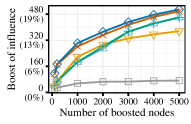
(a) Digg

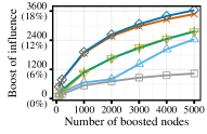
(b) Flixster

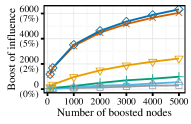
(c) Twitter

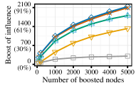
(d) Flickr

Figure 5: Boost of the influence versus $k$ (influential seeds).

Running time. Figure 6 shows the running time of PRR-Boost and PRR-Boost-LB. The running time of both algorithm increases when $k$ increases. This is mainly because the number of random PRR-graphs required increases when $k$ increases. Figure 6 also shows that the running time is in general proportional to the number of nodes and edges for Digg, Flixster and Twitter, but not for Flickr. This is mainly because of the significantly smaller average influence probabilities on Flickr as shown in Table 1, and the accordingly significantly lower expected cost for generating a random PRR-graph (i.e., $EPT$) as we will show shortly in Table 2. In Figure 6, we also label the speedup of PRR-Boost-LB compared with PRR-Boost. Together with Figure 5, we can see that PRR-Boost-LB returns solutions with quality comparable to PRR-Boost but runs faster. Because our approximation algorithms consistently outperform all heuristic methods with no performance guarantee in all tested cases, we do not compare the running time of our algorithms with heuristic methods to avoid cluttering the results.

(a)

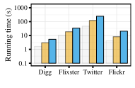
(a) PRR-Boost

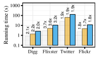
(b) PRR-Boost-LB

Figure 6: Running time (influential seeds).

Effectiveness of the compression phase. Table 2 shows the “compression ratio” of PRR-graphs and memory usages of PRR-Boost and PRR-Boost-LB, demonstrating the importance of compressing PRR-graphs. The compression ratio is the ratio between the average number of uncompressed edges and average number of edges after compression in boostable PRR-graphs. Besides the total memory usage, we also show in parenthesis the memory usage for storing boostable PRR-graphs, which is measured as the additional memory usage starting from the generation of the first PRR-graph. For example, for the Digg dataset and $k=100$, for boostable PRR-graphs, the average number of uncompressed edges is $1810.32$, the average number of compressed edges is $2.41$, and the compression ratio is $751.59$. Moreover, the total memory usage of PRR-Boost is $0.07$GB with around $0.01$GB being used to storing “boostable” PRR-graphs. The compression ratio is high in practice for two reasons. First, many nodes visited in the first phase cannot be reached by seeds. Second, among the remaining nodes, many of them can be merged into the super-seed node, and most non-super-seed nodes will be removed because they are not on any paths to the root node without going through the super-seed node. The high compression ratio and the memory used for storing compressed PRR-graphs show that the compression phase is indispensable. For PRR-Boost-LB, the memory usage is much lower because we only store “critical nodes” of boostable PRR-graphs. In our experiments with $\beta=2$, each boostable PRR-graph only has a few critical nodes on average, which explains the low memory usage of PRR-Boost-LB. If one is indifferent about the slightly difference between the quality of solutions returned by PRR-Boost-LB and PRR-Boost, we suggest to use PRR-Boost-LB because of its lower running time and lower memory usage.

Table 2: Memory usage and compression ratio (influential seeds). Numbers in parentheses are additional memory usage for boostable PRR-graphs.

$k$	Dataset	PRR-Boost		PRR-Boost-LB
		Compression Ratio	Memory (GB)	Memory (GB)
100	Digg	1810.32 / 2.41 = 751.79	0.07 (0.01)	0.06 (0.00)
	Flixster	3254.91 / 3.67 = 886.90	0.23 (0.05)	0.19 (0.01)
	Twitter	14343.31 / 4.62 = 3104.61	0.74 (0.07)	0.69 (0.02)
	Flickr	189.61 / 6.86 = 27.66	0.54 (0.07)	0.48 (0.01)
5000	Digg	1821.21 / 2.41 = 755.06	0.09 (0.03)	0.07 (0.01)
	Flixster	3255.42 / 3.67 = 886.07	0.32 (0.14)	0.21 (0.03)
	Twitter	14420.47 / 4.61 = 3125.37	0.89 (0.22)	0.73 (0.06)
	Flickr	189.08 / 6.84 = 27.64	0.65 (0.18)	0.50 (0.03)

Approximation factors in the Sandwich Approximation. Recall that the approximate ratio of PRR-Boost and PRR-Boost-LB depends on the ratio $\frac{\mu(B^{*})}{\Delta_{S}(B^{*})}$. The closer to one the ratio is, the better the approximation guarantee is. With $B^{*}$ being unknown due to the NP-hardness of the problem, we show the ratio when the boost is relatively large. We obtain $300$ sets of $k$ boosted nodes by replacing a random number of nodes in $B_{sa}$ by other non-seed nodes, where $B_{sa}$ is the solution returned by PRR-Boost. For a given set $B$, we use PRR-graphs generated for finding $B_{sa}$ to estimate $\frac{\mu(B)}{\Delta_{S}(B)}$. Figure 7 shows the ratios for generated sets $B$ as a function of $\Delta_{S}(B)$ for varying $k$. Because we intend to show the ratio when the boost of influence is large, we do not show points corresponding to sets whose boost of influence is less than $50\%$ of $\Delta_{S}(B_{sa})$. For all datasets, the ratio is above $0.94$, $0.83$ and $0.74$ for $k=100,1000,5000$, respectively. The ratio is closer to one when $k$ is smaller, and we now explain this. In practice, most boostable PRR-graphs have “critical nodes”. When $k$ is small, say $100$, PRR-Boost and PRR-Boost-LB tend to return node sets $B$ so that every node in $B$ is a critical node in many boostable PRR-graphs. For example, for Twitter, when $k=100$, among PRR-graphs that have critical nodes and are activated upon boosting $B_{sa}$, above $98\%$ of them have their critical nodes boosted (i.e., in $B_{sa}$). Meanwhile, many root node $r$ of PRR-graphs without critical nodes may stay inactive. For a given PRR-graph $R$, if $B$ contains critical nodes of $R$ or if the root node of $R$ stays inactive upon boosting $B$, $f^{-}_{R}(B)$ does not underestimate $f_{R}(B)$. Therefore, when $k$ is smaller, the ratio of $\frac{\mu(B)}{\Delta_{S}(B)}=\frac{\mathbb{E}[f_{R}^{-}(B)]}{\mathbb{E}[f_{R}(B)]}$ tends to be closer to one. When $k$ increases, we can boost more nodes, and root nodes of PRR-graphs without critical nodes may be activated, thus the approximation ratio tends to decrease. For example, for Twitter, when $k$ increases from $100$ to $5000$, among PRR-graphs whose root nodes are activated upon boosting $B_{sa}$, the fraction of them having critical nodes decreases from around $98\%$ to $88\%$. Accordingly, the ratio of $\mu(B_{sa})/\Delta_{S}(B_{sa})$ decreased by around $9\%$ when $k$ increases from $100$ to $5000$.

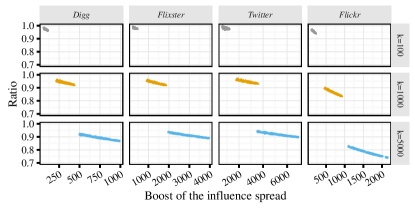
Figure 7: Sandwich Approximation: $\frac{\mu(B)}{\Delta_{S}(B)}$ (influential seeds).

Effects of the boosted influence probabilities. In our experiments, the larger the boosting parameter $\beta$ is, the larger the boosted influence probabilities on edges are. Figure 8 shows the effects of $\beta$ on the boost of influence and the running time when $k=1000$. For other values of $k$, the results are similar. In Figure 8a, the optimal boost increases when $\beta$ increases. When $\beta$ increases, for Flixster and Flickr, PRR-Boost-LB returns solution with quality comparable to those returned by PRR-Boost. For Twitter, we consider the slightly degenerated performance of PRR-Boost-LB acceptable because PRR-Boost-LB runs significantly faster. Figure 8b shows the running time for PRR-Boost and PRR-Boost-LB. When $\beta$ increases, the running time of PRR-Boost increases accordingly, but the running time of PRR-Boost-LB remains almost unchanged. Therefore, compared with PRR-Boost, PRR-Boost-LB is more scalable to larger boosted influence probabilities on edges. In fact, when $\beta$ increases, a random PRR-graph tends to include more nodes and edges. The running time of PRR-Boost increases mainly because the cost for PRR-graph generation increases. However, when $\beta$ increases, we observe that the cost for obtaining “critical nodes” for a random PRR-graph does not change much, thus the running time of PRR-Boost-LB remains almost unchanged. Figure 9 shows the approximation ratio of the sandwich approximation strategy with varying boosting parameters. We observe that, for every dataset, when we increase the boosting parameter, the ratio of $\frac{\mu(B)}{\Delta_{S}(B)}$ for large $\Delta_{S}(B)$ remains almost the same. This suggests that both our proposed algorithms remain effective when we increase the boosted influence probabilities on edges.

(a)

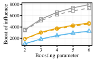
(a) Boost of influence

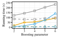
(b) Running time

Figure 8: Effects of the boosting parameter (influential seeds, $k=1000$).

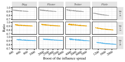
Figure 9: Sandwich Approximation with varying boosting parameter: $\frac{\mu(B)}{\Delta_{S}(B)}$ (influential seeds, $k=1000$).

VII-B Random seeds

In this part, we select five sets of $500$ random nodes as seeds for each dataset. The setting here maps to the real situation where some users become seeds spontaneously. All experiments are conducted on five sets of random seeds, and we report the average results.

Quality of solution. We select up to $5000$ nodes and compare our algorithms with baselines. From Figure 10, we can draw conclusions similar to those drawn from Figure 5 where the seeds are highly influential users. Both PRR-Boost and PRR-Boost-LB outperform all baselines.

(a)

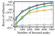
(a) Digg

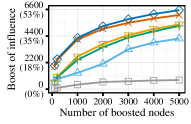
(b) Flixster

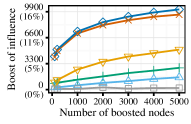
(c) Twitter

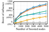
(d) Flickr

Figure 10: Boost of the influence versus $k$ (random seeds).

Running time. Figure 11 shows the running time of PRR-Boost and PRR-Boost-LB, and the speedup of PRR-Boost-LB compared with PRR-Boost. Figure 11b shows that PRR-Boost-LB runs up to three times faster than PRR-Boost. Together with Figure 10, PRR-Boost-LB is in fact both efficient and effective given randomly selected seeds.

(a)

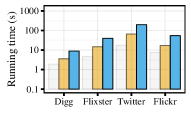
(a) PRR-Boost

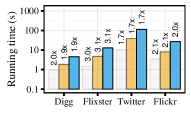
(b) PRR-Boost-LB

Figure 11: Running time (random seeds).

Effectiveness of the compression phase. Table 3 shows the compression ratio of PRR-Boost, and the memory usage of both proposed algorithms. Given randomly selected seed nodes, the compression step of PRR-graphs is also very effective. Together with Table 2, we can conclude that the compression phase is an indispensable step for both cases where the seeds are highly influence users or random users.

Table 3: Memory usage and compression ratio (random seeds).

$k$	Dataset	PRR-Boost		PRR-Boost-LB
		Compression Ratio	Memory (GB)	Memory (GB)
100	Digg	3069.15 / 5.61 = 547.28	0.07 (0.01)	0.06 (0.00)
	Flixster	3754.43 / 25.83 = 145.37	0.24 (0.06)	0.19 (0.01)
	Twitter	16960.51 / 56.35 = 300.96	0.78 (0.11)	0.68 (0.01)
	Flickr	701.84 / 18.12 = 38.73	0.56 (0.09)	0.48 (0.01)
5000	Digg	3040.94 / 5.59 = 544.19	0.12 (0.06)	0.07 (0.01)
	Flixster	3748.74 / 25.86 = 144.94	0.71 (0.53)	0.21 (0.03)
	Twitter	16884.86 / 57.29 = 294.72	1.51 (0.84)	0.72 (0.05)
	Flickr	701.37 / 18.10 = 38.75	1.00 (0.53)	0.50 (0.03)

Approximation factors in the Sandwich Approximation. The approximate ratio of PRR-Boost and PRR-Boost-LB depends on the ratio $\frac{\mu(B^{*})}{\Delta_{S}(B^{*})}$. We use the same method to generate different sets of boosted nodes $B$ as in the previous sets of experiments. Figure 12 shows the ratios for generated sets $B$ as a function of $\Delta_{S}(B)$ for $k\in\{100,1000,5000\}$. For all four datasets, the ratio is above $0.76$, $0.62$ and $0.47$ for $k=100,1000,5000$, respectively. As from Figure 7, the ratio is closer to one when $k$ is smaller. Compared with Figure 7, we observe that the ratios in Figure 12 are lower. The main reason is that, along with many PRR-graphs with critical nodes, many PRR-graphs without critical nodes are also boosted. For example, for Twitter, when $k=5000$, among PRR-graphs whose root nodes are activated upon boosting $B_{sa}$, around $25\%$ of them do not have critical nodes, and around $3\%$ of them have critical nodes but their critical nodes are not in $B_{sa}$. Note that, although the approximation guarantee of our proposed algorithms decreases as $k$ increases, Figure 10 shows that our proposed algorithms still outperform all other baselines.

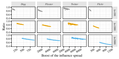
Figure 12: Sandwich Approximation: $\frac{\mu(B)}{\Delta_{S}(B)}$ (random seeds).

VII-C Budget allocation between seeding and boosting

In this part, we vary both the number of seeders and the number of boosted nodes. Under the context of viral marketing, this corresponds to the situation where a company can decide both the number of free samples and the number of coupons they offer. Intuitively, targeting a user as a seeder (e.g., offering a free product and rewarding for writing positive opinions) must cost more than boosting a user (e.g., offering a discount or displaying ads). In the experiments, we assume that we can target $100$ users as seed nodes with all the budget. Moreover, we assume that targeting a seeder costs $100$ to $800$ times as much as boosting a user. For example, suppose targeting a seeder costs $100$ times as much as boosting a user: we can choose to spend $20\%$ of our budget on targeting initial adopters (i.e., finding $20$ seed users and boosting $8000$ users); or, we can spend $80\%$ of the budget on targeting initial adopters (i.e, finding $80$ seeds and boosting $2000$ users). We explore how the expected influence spread changes, when we decrease the number of seed users and increase the number of boosted users. Given the budget allocation (i.e., the number of seeds and the number boosted users), we first identify a set of influential seeds using the IMM method, then we use PRR-Boost to select the set of nodes we boost. Finally, we use $20,000$ Monte-Carlo simulations to estimate the expected boosted influence spread.

(a)

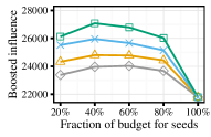
(a) Flixster

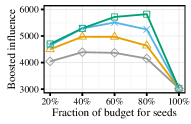
(b) Flickr

Figure 13: Budget allocation between seeding and boosting.

Figure 13 shows the results for Flixster and Flickr. Spending a mixed budget among initial adopters and boosting users achieves higher final influence spread than spending all budget on initial adopters. For example, for cost ratio of $800$ between seeding and boosting, if we choose $80\%$ budget for seeding and $20\%$ for boosting, we would achieve around $20\%$ and $92\%$ higher influence spread than pure seeding, for Flixster and Flickr respectively. Moreover, the best budget mix is different for different networks and different cost ratio, suggesting the need for specific tuning and analysis for each case.

VIII Experiments on Bidirected Trees

We conduct extensive experiments to test the proposed algorithms on bidirected trees. In our experiments, DP-Boost can efficiently approximate the $k$-boosting problem for bidirected trees with thousands of nodes. We also show that Greedy-Boost returns solutions that are near-optimal. All experiments were conduct on same environment as in Section VII.

We use synthetic bidirected trees to test algorithms for bidirected trees in Section VI. For every given number of nodes $n$, we construct a complete (undirected) binary tree with $n$ nodes, then we replace each undirected edge by two directed edges, one in each direction. We assign influence probabilities $\{p_{uv}\}$’s on edges according to the Trivalency model. Moreover, for every edge $e_{uv}$, let $p^{\prime}_{uv}=1-{(1-p_{uv})}^{2}$. For every tree, we select $50$ seeds using the IMM method. We compare Greedy-Boost and DP-Boost. The boost of influence of the returned sets are computed exactly. We run each experiment five times with randomly assigned influence probabilities and report the averaged results.

Greedy-Boost versus DP-Boost with varying $\epsilon$. For DP-Boost, the value of $\epsilon$ controls the tradeoff between the accuracy and computational costs. Figure 14 shows results for DP-Boost with varying $\epsilon$ and Greedy-Boost. For DP-Boost, when $\epsilon$ increases, the running time decreases dramatically, but the boost is almost unaffected. Because DP-Boost returns $(1-\epsilon)$-approximate solutions, it provides a benchmark for the greedy algorithm. Figure 14a shows that the greedy algorithm Greedy-Boost returns near-optimal solutions in practice. Moreover, Figure 14b shows Greedy-Boost is orders of magnitude faster than DP-Boost with $\epsilon=1$ where the theoretical guarantee is in fact lost.

(a)

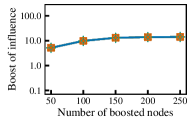
(a) Boost of influence

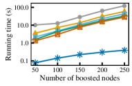
(b) Running time

Figure 14: The greedy algorithm versus the rounded dynamic programming on random bidirected trees with $2000$ nodes.

Greedy-Boost versus DP-Boost with varying tree sizes. We set $\epsilon=0.5$ for DP-Boost. Figure 15 compares Greedy-Boost and DP-Boost for trees with varying sizes. Results for smaller values of $k$ are similar. In Figure 15a, for every $k$, lines representing Greedy-Boost and DP-Boost are completely overlapped, suggesting that Greedy-Boost always return near-optimal solutions on trees with varying sizes. Figure 15b demonstrates the efficiency of Greedy-Boost. Both Figure 14 and Figure 15 suggest that Greedy-Boost is very efficient and it returns near-optimal solutions in practice.

(a)

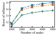
(a) Boost of influence

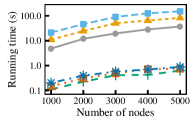
(b) Running time

Figure 15: The greedy algorithm versus the rounded dynamic programming on random bidirected trees with varies sizes.

IX Conclusion

In this work, we address a novel $k$-boosting problem that asks how to boost the influence spread by offering $k$ users incentives so that they are more likely to be influenced by friends. For the $k$-boosting problem on general graphs, we develop efficient approximation algorithms, PRR-Boost and PRR-Boost-LB, that have data-dependent approximation factors. Both PRR-Boost and PRR-Boost-LB are delicate integration of Potentially Reverse Reachable Graphs and the state-of-the-art techniques for influence maximization problems. For the $k$-boosting problem on bidirected trees, we present an efficient greedy algorithm Greedy-Boost based on a linear-time exact computation of the boost of influence spread, and we also present DP-Boost which is shown to be a fully polynomial-time approximation scheme. We conduct extensive experiments on real datasets using PRR-Boost and PRR-Boost-LB. In our experiments, we consider both the case where the seeds are highly influential users, and the case where the seeds are randomly selected users. Results demonstrate the superiority of our proposed algorithms over intuitive baselines. Compared with PRR-Boost, experimental results show that PRR-Boost-LB returns solution with comparable quality but has significantly lower computational costs. On real social networks, we also explore the scenario where we are allowed to determine how to spend the limited budget on both targeting initial adopters and boosting users. Experimental results demonstrate the importance of studying the problem of targeting initial adopters and boosting users with a mixed strategy. We also conduct experiments on synthetic bidirected trees using Greedy-Boost and DP-Boost. Results show the efficiency and effectiveness of our Greedy-Boost and DP-Boost. In particular, we show via experiments that Greedy-Boost is extremely efficient and returns near-optimal solutions in practice.

The proposed “boosting” problem has several more future directions. One direction is to design more efficient approximation algorithms or effective heuristics for the $k$-boosting problem. This may requires new techniques about how to tackle the non-submodularity of the objective function. These new techniques may also be applied to solve other existing or future questions in the area of influence maximization. Another direction is to investigate similar problems under other influence diffusion models, for example the well-known Linear Threshold (LT) model. We believe the general question of to how to boost the spread of information is of great importance and it deserves more attention.

Appendix A Proofs

See 1

Lemma 8 proves the NP-hardness of the $k$-boosting problem, and Lemma 9 shows the #P-hardness of the boost computation.

Lemma 8.

The $k$-boosting problem is NP-hard.

Figure 16: Illustration of the NP-hardness graph construction: $X=\{x_{1},x_{2},\ldots,x_{6}\}$, $\mathcal{C}=\{C_{1},C_{2},C_{3}\}$, $C_{1}=\{x_{1},x_{2},x_{3}\}$, $C_{2}=\{x_{2},x_{3},x_{4}\}$, $C_{3}=\{x_{4},x_{5},x_{6}\}$, with $m=3$, $n=6$.

Proof.

We prove Lemma 8 by a reduction from the NP-complete Set Cover problem [25]. The Set Cover problem is as follows: Given a ground set $X=\{e_{1},e_{1},\ldots,e_{n}\}$ and a collection $\mathcal{C}$ of subsets $\mathcal{C}=\{C_{1},C_{2},\ldots,C_{m}\}$ of $X$, we want to know whether there exist $k$ subsets in $\mathcal{C}$ so that their union is $X$. We assume that every element in $X$ is covered by at least one set in $\mathcal{C}$. We reduce the Set Cover problem to the $k$-boosting problem as follows.

Given an arbitrary instance of the Set Cover problem. We define a corresponding directed tripartite graph $G$ with $1+m+n$ nodes. Figure 16 shows how we construct the graph $G$. Node $s$ is a seed node. Node set $V_{C}=\{c_{1},c_{2},\ldots,c_{m}\}$ contains $m$ nodes, where node $c_{i}$ corresponds to the set $C_{i}$ in $\mathcal{C}$. Node set $V_{X}=\{x_{1},x_{2},\ldots,x_{n}\}$ contains $n$ nodes, where node $x_{i}$ corresponds to the element $e_{i}$ in $X$. For every node $c_{i}\in V_{C}$, there is a directed edge from $s$ to $c_{i}$ with an influence probability of $0.5$ and a boosted influence probability of $1$. Moreover, if a set $C_{i}$ contains an element $e_{j}$ in $X$, we add a directed edge from $c_{i}$ to $x_{j}$ with both the influence probability and the boosted influence probability on that edge being $1$. Denote the degree of the node $x_{i}\in V_{X}$ by $d_{x_{i}}$. When we do not boost any nodes in $G$ (i.e., $B=\emptyset$), the expected influence spread of $S=\{s\}$ in $G$ can be computed as $\sigma_{S}(\emptyset)=1+m+\sum_{x_{i}\in V_{X}}\Big{(}1-{0.5}^{d_{x_{i}}}\Big{)}$. The Set Cover problem is equivalent to deciding if there is a set $B$ of $k$ boosted nodes in graph $G$ so that $\sigma_{S}(B)=\sigma_{S}(\emptyset)+\Delta_{S}(B)=1+n+m$. Because the Set Cover problem [25] is NP-complete, the $k$-boosting problem is NP-hard. ∎

Lemma 9.

Computing $\Delta_{S}(B)$ given $S$ and $B$ is #P-hard.

Figure 17: Illustration of the #P-hardness graph construction.

Proof.

We prove Lemma 9 by a reduction from the #P-complete counting problem of $s$-$t$ connectedness in a directed graph [26]. An instance of the $s$-$t$ connectedness is a directed graph $G_{1}=(V,E)$ and two nodes $s$ and $t$ in the graph. The problem is to count the number of subgraphs of $G_{1}$ in which $s$ is connected to $t$. This problem is equivalent to computing the probability that $s$ is connected to $t$ when each edge in $G_{1}$ has an independent probability of $0.5$ to be connected, and another $0.5$ to be disconnected.

We reduce this problem to the computation of the boost of influence spread. Let $G_{2}=(V\cup\{t^{\prime}\},E\cup\{e_{tt^{\prime}}\})$ be a directed graph. Figure 17 shows the construction of $G_{2}$. In $G_{2}$, let $S=\{s\}$, $B=\{t^{\prime}\}$. Moreover, let $p_{uv}=0.5$ and $p^{\prime}_{uv}=1$ for every edge $e_{uv}$ in $G_{2}$. We compute $\Delta_{S}(B)$ for graph $G_{2}$. Then, $\Delta_{S}(B)/(p_{tt^{\prime}}^{\prime}-p_{tt^{\prime}})=2\Delta_{S}(B)$ is the probability that $s$ is connected to $t$ in $G_{1}$, when each edge in $G_{1}$ has an independent probability of $0.5$ to be connected. Thus, we solve the $s$-$t$ connectedness counting problem. Because the $s$-$t$ connectedness problem is #P-complete, the computation of the boost of influence spread (i.e., $\Delta_{S}(B)$) is #P-hard. ∎

See 4

Proof.

Let $B$ be a boost set with $k$ nodes, we say that $B$ is a bad set if $\Delta_{S}(B)<(1-1/e-\epsilon)\cdot OPT_{\mu}$. To prove Lemma 4, we first show that each bad boost set with $k$ nodes is returned by Algorithm 2 with a probability of at most $(1-n^{-\ell^{\prime}})/\binom{n}{k}$. Let $B$ be an arbitrary bad set with $k$ nodes, we have

$$\Delta_{S}(B)<(1-1/e-\epsilon)\cdot OPT_{\mu}.$$ (14)

If we return $B$ as the $B_{sa}$, we must have $\hat{\Delta}_{\mathcal{R}}(B)>\hat{\Delta}_{\mathcal{R}}(B_{\mu})$. Therefore, the probability that $B$ is returned is upper bounded by $\Pr[\hat{\Delta}_{\mathcal{R}}(B)>\hat{\Delta}_{\mathcal{R}}(B_{\mu})]$. From Equation 6 and Equation 14, we have

$$n\cdot\hat{\mu}_{\mathcal{R}}(B_{\mu})-\Delta_{S}(B)$$

$$\geq (1-1/e)\cdot(1-\epsilon_{1})\cdot OPT_{\mu}-(1-1/e-\epsilon)\cdot OPT_{\mu}$$

$$= (\epsilon-(1-1/e)\cdot\epsilon_{1})\cdot OPT_{\mu}.$$

Let $\epsilon_{2}=\epsilon-(1-1/e)\cdot\epsilon_{1}$, we have

$$\Pr[\hat{\Delta}_{\mathcal{R}}(B)>\hat{\Delta}_{\mathcal{R}}(B_{\mu})]$$

$$\leq \Pr[\hat{\Delta}_{\mathcal{R}}(B)>\hat{\mu}_{\mathcal{R}}(B_{\mu})]$$

$$\leq \Pr[n\cdot\hat{\Delta}_{\mathcal{R}}(B)-\Delta_{S}(B)>n\cdot\hat{\mu}_{\mathcal{R}}(B_{\mu})-\Delta_{S}(B)]$$

$$\leq \Pr[n\cdot\hat{\Delta}_{\mathcal{R}}(B)-\Delta_{S}(B)>\epsilon_{2}\cdot OPT_{\mu}].$$

Let $p=\Delta_{S}(B)/n$, we know $p=\mathbb{E}[f_{R}(B)]$ from Lemma 1. Recall that $\theta\!=\!|\mathcal{R}|$ and $\hat{\Delta}_{\mathcal{R}}(B)\!=\!\big{(}\sum_{R\in\mathcal{R}}f_{R}(B)\big{)}/\theta$. Let $\delta=\frac{\epsilon_{2}\cdot OPT_{\mu}}{np}$, by Chernoff bound, we have

$$\Pr\left[n\cdot\hat{\Delta}_{\mathcal{R}}(B)-\Delta_{S}(B)>\epsilon_{2}\cdot OPT_{\mu}\right]$$

$$= \Pr\left[\sum_{R\in\mathcal{R}}f_{R}(B)-\theta p>\frac{\epsilon_{2}\cdot OPT_{\mu}}{np}\cdot\theta p\right]$$

$$\leq \exp\Big{(}-\frac{\delta^{2}}{2+\delta}\cdot\theta p\Big{)}=\exp\Big{(}-\frac{\epsilon_{2}^{2}\cdot OPT_{\mu}^{2}}{2n^{2}p+\epsilon_{2}\cdot OPT_{\mu}\cdot n}\cdot\theta\Big{)}$$

$$\leq \exp\Big{(}{-}\frac{\epsilon_{2}^{2}{\cdot}OPT_{\mu}^{2}}{2n(1{-}1/e{-}\epsilon){\cdot}OPT_{\mu}{+}\epsilon_{2}{\cdot}OPT_{\mu}{\cdot}n}{\cdot}\theta\Big{)}\text{(by Ineq~{}\eqref{eq:bad_solution})}$$

$$\leq \exp\Big{(}-\frac{(\epsilon-(1-1/e)\cdot\epsilon_{1})^{2}\cdot OPT_{\mu}}{n\cdot(2-2/e)}\cdot\theta\Big{)}$$

$$\leq \exp\Big{(}-\log\big{(}\tbinom{n}{k}\cdot(2n^{\ell^{\prime}})\big{)}\Big{)}\quad\text{(by Ineq~{}\eqref{eq:prr_boost_lb1})}$$

$$\leq n^{-\ell^{\prime}}/\tbinom{n}{k}.$$

Because there are at most $\binom{n}{k}$ bad sets $B$ with $k$ nodes, by union bound, the probability that Algorithm 2 returns a bad solution is at most $n^{-\ell^{\prime}}$. Because $OPT_{\mu}\geq\mu(B^{*})$, the probability that Algorithm 2 returns a solution so that $\Delta_{S}(B_{sa})<(1-1/e-\epsilon)\cdot\mu(B^{*})$ is also at most $n^{-\ell^{\prime}}$. ∎

See 5

Proof.

Suppose we boost the node set $B$. Equation 7 holds from the fact that node $u$ does not get influenced if and only if all its neighbors (i.e., $N(u)$) fail to influence it. Equation 8 holds from the fact that node $u$ does not get influenced if and only if all of its neighbors in $G_{u\backslash v}$ (i.e., $N(u)\backslash\{v\}$) fail to influence it. Equation 9 is a direct result from Equation 8, and we have $1-ap_{B}(v\backslash u)\cdot{}p^{B}_{v,u}>0$ because we have assumed that non-seed nodes are activated with probability less than one. ∎

See 6

Proof.

In $G_{u\backslash v}$, suppose we insert the node $u$ into the seed set. The activation probability of node $u$ itself increases from $ap_{B}(u\backslash v)$ to $1$, increases by $1-ap_{B}(u\backslash v)$. Let node $w$ be a neighbor of $u$ in $G_{u\backslash v}$. The probability that $u$ could be activated by nodes other than $w$ increases from $1-\prod_{x\in N(u)\backslash\{v,w\}}(1-ap_{B}(x\backslash u)\cdot{}p^{B}_{x,u})$ to $1$, increases by

$$\prod_{x\in N(u)\backslash\{v,w\}}\left(1-ap_{B}(x\backslash u)\cdot{}p^{B}_{x,u}\right)=\frac{1-ap_{B}(u\backslash v)}{1-ap_{B}(w\backslash u)\cdot{}p^{B}_{w,u}}.$$

In the above equation, we have $1-ap_{B}(w\backslash u)\cdot{}p^{B}_{w,u}>0$ because we assume that non-seed nodes are activated with probability less than one. By definition of $g_{B}(u\backslash v)$, we have

$$g_{B}(u\backslash v)= \left(1-ap_{B}(u\backslash v)\right)$$

$$+\sum_{\begin{subarray}{c}w\in N(u)\\ w\neq v\end{subarray}}\frac{1-ap_{B}(u\backslash v)}{1-ap_{B}(w\backslash u)\cdot{}p^{B}_{w,u}}\cdot{}p^{B}_{u,w}\cdot g_{B}(w\backslash u),$$

and Lemma 6 holds. Lemma 6 can be derived directly from Lemma 6. ∎

See 7

Proof.

If $u\in B$ or $u\in S$, it is obvious that $\sigma_{S}(B\cup\{u\})=\sigma_{S}(B)$. Now, consider $u\in V\backslash(B\cup S)$, and we insert node $u$ into the boost set $B$. The value of $\Delta ap_{B}(u)$ is the increase of the activation probability of node $u$ itself. The value of $\Delta ap_{B}(u\backslash v)$ is the increase of the activation probabilities of node $u$ in $G_{u\backslash v}$. Suppose $v$ is a neighbor of $u$. Let $V_{v\backslash u}$ be the set of nodes in $G_{v\backslash u}$. In graph $G$, when we insert node $u$ into $B$, the expected number of activated nodes in $V_{v\backslash u}$ increases by ${}p^{B}_{u,v}\cdot\Delta ap_{B}(u\backslash v)\cdot g_{B}(v,u)$. Thus, we have Equation 12 holds. ∎

See 3

The proof of Theorem 3 relies on the following lemma.

Lemma 10.

We have $a_{1}a_{2}-b_{1}b_{2}\leq(a_{1}-b_{1})+(a_{2}-b_{2})$ for $0\leq a_{i}\leq 1$, $0\leq b_{i}\leq 1$.

Proof.

The complexity of DP-Boost has been analyzed in the paper. Let $B^{*}$ be the optimal solution of the $k$-boosting problem, and assume $\Delta_{S}(B^{*})\geq 1$. Let $\tilde{B}$ be the solution returned by DP-Boost. To prove Theorem 3, we only need to prove that we have

$$\Delta_{S}(\tilde{B})\geq(1-\epsilon)\Delta_{S}(B^{*}).$$ (15)

Suppose we boost nodes in $B^{*}$. For every node $v$, let $\kappa_{v}^{*}=|B^{*}\cap T_{v}|$ be the number of nodes boosted in $T_{v}$, let $c_{v}^{*}$ be the probability that node $v$ is activated in $T_{v}$ and let $f_{v}^{*}$ be the probability that node $v$’s parent is activated in $G\backslash T_{v}$. If $v$ is the root node, let $f^{*}_{v}=0$. For every node $v$, let $u$ be the parent of $v$ and let $v_{i}$ be the $i$-th child of $v$, we have

$$g(v,\kappa^{*}_{v},c^{*}_{v},f^{*}_{v})=\Big{(}\sum_{v_{i}}g(v_{i},\kappa^{*}_{v_{i}},c^{*}_{v_{i}},f^{*}_{v_{i}})\Big{)}$$

$$+1-(1-f^{*}_{v}\cdot{}p^{B^{*}}_{u,v})(1-c^{*}_{v})-ap_{\emptyset}(v),$$ (16)

$$\Delta_{S}(B^{*})=\sum_{v\in V}\Big{(}1-(1-f^{*}_{v}\cdot{}p^{B^{*}}_{u,v})(1-c^{*}_{v})-ap_{\emptyset}(v)\Big{)}.$$ (17)

Define $p^{*}(x\rightsquigarrow y)$ as the probability that node $x$ can influence node $y$, given that $B^{*}$ is boosted. If $x=y$, we let $p^{*}(x\rightsquigarrow y)=1$.

We now assign rounded values $\tilde{c}_{v}$ and $\tilde{f}_{v}$ for all node $v$. The assignment guarantees that for every internal node $v$, $(\kappa^{*}_{v_{i}},\tilde{c}_{v_{i}},\tilde{f}_{v_{i}},\forall i)$ is a consistent subproblem of $g^{\prime}(v,\kappa^{*}_{v},\tilde{c}_{v},\tilde{f}_{v})$.

We first assign values $\tilde{c}_{v}$ for every node $v$ in $G$. We will show that for every node $v$ we have

$$c_{v}^{*}-\tilde{c}_{v}\leq\delta\cdot\sum_{x\in T_{v}}p^{*}(x\rightsquigarrow v).$$ (18)

We assign values of $\tilde{c}$ from leaf nodes to the root node. For a leaf node $v$, let $\tilde{c}_{v}=\big{\lfloor}{c^{*}_{v}}\big{\rfloor}_{\delta}$ and Equation 18 holds. For every internal seed node $v$, let $\tilde{c}_{v}=1$ and Equation 18 holds. For every non-seed internal node $v$, let $\tilde{c}_{v}=\big{\lfloor}{1-\prod_{v_{i}}(1-\tilde{c}_{v_{i}}\cdot{}p^{B^{*}}_{v_{i},v})}\big{\rfloor}_{\delta}$, and Equation 18 can be verified as follows.

$$c^{*}_{v}{-}\tilde{c}_{v}=1{-}\prod_{v_{i}}\left(1{-}c^{*}_{v_{i}}\cdot{}p^{B^{*}}_{v_{i},v}\right){-}\Big{\lfloor}{1{-}\prod_{v_{i}}\left(1{-}\tilde{c}_{v_{i}}\cdot{}p^{B^{*}}_{v_{i},v}\right)}\Big{\rfloor}_{\delta}$$

$$\leq \delta{+}\sum_{v_{i}}(c^{*}_{v_{i}}{-}\tilde{c}_{v_{i}})\cdot{}p^{B^{*}}_{v_{i},v}\leq\delta{+}\sum_{v_{i}}\Big{(}\delta\sum_{x\in T_{v_{i}}}p^{*}(x\rightsquigarrow v_{i})\cdot{}p^{B^{*}}_{v_{i},v}\Big{)}$$

$$\leq \delta\sum_{x\in T_{v}}p^{*}(x\rightsquigarrow v)$$

The first inequality holds from Lemma 10, and the second inequality holds by induction.

Now, we assign values $\tilde{f}_{v}$ for every node $v$ from root to leaf. For every non-root node $v$, denote its parent by $u$, we will show that our assignment satisfies

$$f_{v}^{*}-\tilde{f}_{v}\leq\delta\cdot\sum_{x\in G\backslash T_{v}}p^{*}(x\rightsquigarrow u).$$ (19)

For the root node $r$, we have $f^{*}_{r}=0$, and we let $\tilde{f}_{r}=0$. For an internal seed node $v$ and the $i$-th child $v_{i}$ of $v$, let $\tilde{f}_{v_{i}}=1$ and Equation 19 holds for $v_{i}$ because $f^{*}_{v_{i}}=1$. For an internal non-seed node $v$ and its child $v_{i}$, denote the parent of $v$ by $u$, let $\tilde{f}_{v_{i}}=\Big{\lfloor}{1-(1-\tilde{f}_{v}\cdot{}p^{B^{*}}_{u,v})\prod_{j\neq i}\left(1-\tilde{c}_{v_{j}}\cdot{}p^{B^{*}}_{v_{j},v}\right)}\Big{\rfloor}_{\delta}$. Then, Equation 19 can be verified as follows.

$$f^{*}_{v_{i}}-\tilde{f}_{v_{i}}\leq\delta+(f^{*}_{v}-\tilde{f}_{v})\cdot{}p^{B^{*}}_{u,v}+\sum_{j\neq i}(c^{*}_{v_{j}}-\tilde{c}_{v_{j}})\cdot{}p^{B^{*}}_{v_{j},v}$$

$$\leq\delta+\delta\cdot\sum_{x\in G\backslash T_{v}}p^{*}(x\rightsquigarrow v)+\delta\cdot\sum_{j\neq i}\sum_{x\in T_{v_{j}}}p^{*}(x\rightsquigarrow v)$$

$$\leq\delta\cdot\sum_{x\in G\backslash T_{v_{i}}}p^{*}(x\rightsquigarrow v)$$

The first inequality holds from Lemma 10, and the second inequality holds by induction.

For every internal node $v$, from how we assign the values of $\tilde{c}_{v}$ and $\tilde{f}_{v}$, we can conclude that $(\kappa^{*}_{v_{i}},\tilde{c}_{v_{i}},\tilde{f}_{v_{i}},\forall i)$ is a consistent subproblem of $g^{\prime}(v,\kappa^{*}_{v},\tilde{c}_{v},\tilde{f}_{v})$.

Let $\tilde{B}$ be the set of nodes returned by DP-Boost, we have

$$\Delta_{S}(\tilde{B})\geq\sum_{v\in V}\max\Big{\{}1-(1-\tilde{f}_{v}\cdot{}p^{B^{*}}_{u,v})(1-\tilde{c}_{v})-ap_{\emptyset}(v),0\Big{\}},$$

where we use $u$ to denote the parent of $v$. Moreover, we have

$$\Delta_{S}(B^{*})-\Delta_{S}(\tilde{B})\leq\sum_{v\in V}\big{(}(f^{*}_{v}-\tilde{f}_{v})\cdot{}p^{B^{*}}_{u,v}+(c^{*}_{v}-\tilde{c}_{v})\big{)}$$

$$\leq\delta\sum_{v\in V}\big{(}\!\!\!\!\sum_{x\in G\backslash T_{v}}\!\!\!p^{*}(x\rightsquigarrow v){+}\sum_{x\in T_{v}}p^{*}(x\rightsquigarrow v)\big{)}$$

$$\leq\delta\sum_{v\in V}\sum_{x\in V}p^{*}(x\rightsquigarrow v)\leq\delta\sum_{v\in V}\sum_{x\in V}p^{(k)}(x\rightsquigarrow v).$$

Finally, recall that the rounding parameter $\delta$ of DP-Boost is $\delta=\frac{\epsilon\cdot\max(LB,1)}{\sum_{v\in V}\sum_{x\in V}p^{(k)}(x\rightsquigarrow v)}$, where $LB$ is a lower bound of $\Delta_{S}(B^{*})$. We can conclude that $\Delta_{S}(\tilde{B})\geq(1-\epsilon)\cdot\Delta_{S}(B^{*})$. ∎

Appendix B DP-Boost for General Bidirected Trees

In this section, we extend DP-Boost in Section VI-B to tackle the $k$-boosting problem on general bidirected trees. On general bidirected trees, there is no restriction of the number of children of nodes. For the exact dynamic programming, the description in Section VI-B naturally works for general bidirected trees. However, the generalization of DP-Boost is non-trivial and the definition of consistent subproblem is much more involved. Formally, the general DP-Boost is as follows.

Definition 5 (General DP-Boost).

Let $v$ be a node. Denote the parent node of $v$ by $u$.

• Base case. Suppose $v$ is a leaf node. If $c\neq\mathbb{I}({v\in S})$, let $g^{\prime}(v,\kappa,c,f)=-\infty$; otherwise, let

  $$g^{\prime}(v,\kappa,c,f)=\max\big{\{}1{-}(1{-}c)(1{-}f\cdot{}p^{\mathbb{I}({\kappa>0})}_{u,v}){-}ap_{\emptyset}(v),0\big{\}}.$$

• Recurrence formula. Suppose $v$ is an internal node. If $v$ is a seed node, we let $g^{\prime}(v,\kappa,c,f)=-\infty$ for $c\neq 1$, and let

  $$g^{\prime}(v,\kappa,1,f)=\max_{\kappa=\sum\kappa_{v_{i}}}\sum_{i}g^{\prime}(v_{i},\kappa_{v_{i}},c_{v_{i}},1).$$

  If $v$ is a non-seed node with $d\geq 1$ children. We use $C^{\prime}(v,\kappa,c,f)$ to denote the set of consistent subproblems of $g^{\prime}(v,\kappa,c,f)$. For $1\leq i\leq d$, define

  $$\delta_{v}(i)=\begin{cases}\frac{\delta}{d-2}&1<i<d,\\ 0&\text{otherwise}.\end{cases}$$

  Subproblems $(\kappa_{v_{i}},c_{v_{i}},f_{v_{i}},\forall i)$ are consistent with $g^{\prime}(v,\kappa,c,f)$ if they satisfy the following conditions.

  • About $\kappa$ and $\kappa_{v_{i}}$: $\kappa=\sum_{v_{i}}\kappa_{v_{i}}+b$ where $b\in\{0,1\}$.

  • About $c$ and $c_{v_{i}}$: $c=\big{\lfloor}{x_{d}}\big{\rfloor}_{\delta}$, where $x_{0}=0$ and $x_{i}=\Big{\lfloor}{1-(1-x_{i-1})(1-c_{v_{i}}\cdot{}p^{b}_{v_{i},v})}\Big{\rfloor}_{\delta_{v}(i)}$ for $1\leq i\leq d$.

  • About $f$ and $f_{v_{i}}$: $f_{v_{i}}=\Big{\lfloor}{1-(1-x_{i-1})(1-y_{i})}\Big{\rfloor}_{\delta}$ for $1\leq i\leq d$, where $y_{d}=f\cdot{}p^{b}_{u,v}$ and $y_{i}=\Big{\lfloor}{1-(1-y_{i+1})(1-c_{v_{i+1}}\cdot{}p^{b}_{v_{i+1},v})}\Big{\rfloor}_{\delta_{v}(i)}$ for $1\leq i\leq d$.

  If $C^{\prime}(v,\kappa,c,f)=\emptyset$, let $g^{\prime}(v,\kappa,c,f)=\!-\!\infty$; otherwise, let

  $$g^{\prime}(v,\kappa,c,f)=\!\!\!\!\!\!\!\max_{\begin{subarray}{c}(\kappa_{v_{i}},f_{v_{i}},c_{v_{i}},\forall i)\\ \in C^{\prime}(v,\kappa,c,f),\\ b=k-\sum_{i}\kappa_{v_{i}}\end{subarray}}\left(\begin{subarray}{c}\sum_{i}g^{\prime}(v_{i},\kappa_{v_{i}},c_{v_{i}},f_{v_{i}})+\\ \max\{1{-}(1{-}c)(1{-}f\cdot{}p^{b}_{u,v}){-}ap_{\emptyset}(v),0\}\end{subarray}\right).$$

For a bidirected tree where every node has at most two children, Definition 5 degenerates to Definition 4. Definition 5 defines consistent subproblems of $g^{\prime}(v,\kappa,c,f)$, with some intermediate variables $x_{i}$ and $y_{i}$. Intuitively, when there is no rounding, $x_{i}$ is the probability that $v$ is activated in $T_{v}\backslash(\cup_{j>i}T_{v_{j}})$, and $y_{i}$ is the probability that $v$ is activated in $G\backslash(\cup_{j\leq i}T_{v_{j}})$. To prevent the number of possible values of $x_{i}$ and $y_{i}$ from growing exponentially with $d$, we also round $x_{i}$ and $y_{i}$ for all $1<i<d$.

Algorithm 4 depicts the framework of the general DP-Boost. First, Lines 4-4 determine the rounding parameter $\delta$. With the rounding parameter $\delta$, we compute the values of $g^{\prime}(\ldots)$ bottom-up. There are four subroutines that compute the values of $g^{\prime}(v,\ldots)$ for different types of nodes. We will describe each subroutine in detail. For notational convenience, in the remaining of this section, we use $u$ to denote the parent of node $v$ when the context is clear.

1 $B_{greedy}=\textit{Greedy-Boost}(G,S,k)$

$\delta=\frac{\epsilon\cdot\max(\Delta_{S}(B_{greedy}),1)}{2\sum_{v\in V}\sum_{x\in V}p^{(k)}(x\rightsquigarrow v)}$

  // rounding parameter

2 for nodes $v$ from leaf to root do // compute $g^{\prime}(\dots)$

3     if $v$ is a leaf then Leaf($v$)

4     else if $v$ is a seed then InternalSeed($v$)

5     else if $v$ has non child then NonseedWithChild($v$)

6     else NonseedWithChildren($v$)

7     

8return node set $B$ corresponding to $\max_{c}g^{\prime}(r,k,c,0)$

Algorithm 4 General DP-Boost $(G,S,k,\epsilon)$

Leaf($v$): Suppose node $v$ is a leaf node, we assign $g^{\prime}(v,\kappa,c,f)$ for all $\kappa$, and rounded value of $c$ and $f$ by Definition 5. There are $O(k/\delta^{2})$ entries, assigning each entry takes $O(1)$ time. Thus, the complexity of this subroutine is $O(k/\delta^{2})$.

InternalSeed($v$): Suppose node $v$ is a internal seed node with $d$ children ($d\geq 1$). We first initialize $g^{\prime}(v,\kappa,c,f)=-\infty$ for all $\kappa$ and rounded values of $c$ and $f$. Because $v$ is a seed node, node $v$ is activated in $T_{v}$ with probability $c=1$ and we must have $f_{v_{i}}=1$ for the $i$-th child $v_{i}$ of $v$. However, the number of assignments of $(\kappa_{v_{i}},c_{v_{i}},f_{v_{i}}=1,\forall i)$ can still grow exponentially with the number of children, because $c_{v_{i}}$ for each children $v_{i}$ could have up to $1/\delta$ possible values. To tackle this problem, we define a helper function $h(i,\kappa)$ for $1\leq i\leq d$ and $0\leq\kappa\leq k$. When there is no rounding, the value of $h(i,\kappa)$ is the maximum increase of the expected number of activated nodes in $\cup_{j\leq i}T_{v_{j}}$ (i.e., the first $i$ subtrees of $v$), given that we boost at most $\kappa$ nodes in the first $i$ subtrees of $v$. Formally, $h(i,\kappa)$ is defined as follows:

$$h(i,\kappa)= \max_{\kappa=\sum_{j=1}^{i}\kappa_{j}}\left\{\sum_{j=1}^{i}\max_{c_{v_{j}}}\big{\{}g^{\prime}(v_{j},\kappa_{v_{j}},c_{v_{j}},1)\big{\}}\right\}.$$

Assuming $h(0,\kappa)=0$ for all $\kappa$. The value of $h(i,\kappa)$ for $i>1$ can be efficiently computed as follows:

$$h(i,\kappa)= \max_{0\leq\kappa_{v_{i}}\leq\kappa}\left\{h(i-1,\kappa-\kappa_{v_{i}})+\max_{c_{v_{i}}}g^{\prime}(v_{i},\kappa_{v_{i}},c_{v_{i}},1)\right\}.$$ (20)

Algorithm 5 depicts InternalSeed($v$). The complexity of this subroutine is $O(d\cdot k\cdot(k+1/\delta))$.

1 Initialize $g^{\prime}(v,\kappa,c,f)\leftarrow-\infty$ for all $0\leq\kappa\leq k$ and rounded $c$ and $f$

2Initialize $h(i,\kappa)\leftarrow 0$, for $0\leq i\leq d$ and $0\leq\kappa\leq k$

3for $i\leftarrow 1$ to $d$ do // $d$ is the number of children of $v$

4      for $\kappa_{v_{i}}\leftarrow 0$ to $k$ do

            $\text{max}_{g}\leftarrow\max_{c_{v_{i}}}g^{\prime}(v_{i},\kappa_{v_{i}},c_{v_{i}},1)$

              // $f_{v_{i}}=1$

5            for $\kappa\leftarrow\kappa_{v_{i}}$ to $k$ do

6                  $h(i,\kappa)=\max\big{\{}h(i,\kappa),h(i-1,\kappa-\kappa_{v_{i}})+\text{max}_{g}\big{\}}$

7            

8      

9forall $0\leq\kappa\leq k$ and rounded $f$ do

      $g^{\prime}(v,\kappa,1,f)\leftarrow h(d,\kappa)$

        // boost $\kappa$ nodes among the first $d$ subtrees

10      

Algorithm 5 InternalSeed($v$)

NonseedWithChild($v$): Suppose $v$ is a non-seed node with one child. We first initialize $g^{\prime}(v,\kappa,c,f)=-\infty$ for all $\kappa$ and rounded values of $c$ and $f$. Then, we compute $g^{\prime}(v,\kappa,c,f)$ by Definition 5. Algorithm 6 depicts this subroutine. The complexity of this subroutine is $O(k/\delta^{2})$.

1 Initialize $g^{\prime}(v,\kappa,c,f)\leftarrow-\infty$ for all $0\leq\kappa\leq k$ and rounded $c$ and $f$

2forall $b\in\{0,1\}$, rounded $c_{v_{1}},f$ do

3      $c\leftarrow\big{\lfloor}{c_{v_{1}}\cdot{}p^{b}_{v_{1},v}}\big{\rfloor}_{\delta}$, $f_{v_{1}}\leftarrow\big{\lfloor}{f\cdot{}p^{b}_{u,v}}\big{\rfloor}_{\delta}$

4       $boost_{v}\leftarrow\max\big{\{}1-(1-c)(1-f\cdot{}p^{b}_{u,v})-ap_{\emptyset}(v),0\big{\}}$

5       for $\kappa=b$ to $k$ do

6            $g^{\prime}(v,\kappa,c,f)\leftarrow\max\big{\{}g^{\prime}(v,\kappa,c,f),g^{\prime}(v_{1},\kappa\!-\!b,c_{v_{1}},f_{v_{1}})+boost_{v}\big{\}}$

7      

Algorithm 6 NonseedWithChild($v$)

NonseedWithChildren($v$): Suppose node $v$ is a non-seed node with $d\geq 2$ children. Similar to the subroutine InternalSeed($\cdot$), we need a helper function. Let $h(b,i,\kappa,x_{i},z_{i})$ be the helper function, where $b\in\{0,1\}$, $2\leq i\leq d$. Moreover, for $h(b,i,\kappa,x_{i},z_{i})$, we only consider values of $x_{i}$ and $z_{i}$ that are multiples of $\delta_{v}(i)$. The helper function $h(b,i,\kappa,x_{i},y)$ is formally defined as follows.

$$h(b,i, \kappa,x_{i},z_{i})=\max\quad\sum_{j=1}^{i}g(v_{j},\kappa_{v_{j}},c_{v_{j}},f_{v_{j}})$$

$$s.t.\quad \kappa=\sum_{j=1}^{i}\kappa_{v_{j}}+b,x_{0}=0,$$

$$x_{j}=\Big{\lfloor}{1{-}(1{-}x_{j{-}1})(1{-}c_{v_{j}}\cdot{}p^{b}_{v_{j},v})}\Big{\rfloor}_{\delta_{v}(j)}\ (1\leq j\leq i),$$

$$y_{i}=z_{i}\cdot{}p^{b}_{u,v}\text{ if }i=d\text{ and }y_{i}=z_{i}\text{ otherwise}$$

$$y_{j}=\Big{\lfloor}{1{-}(1{-}y_{j+1})(1{-}c_{v_{j+1}}\cdot{}p^{b}_{v_{j+1},v})}\Big{\rfloor}_{\delta_{v}(j)}(1\leq j<i)$$

$$f_{v_{j}}=\big{\lfloor}{1{-}(1{-}x_{j{-}1})(1{-}y_{j})}\big{\rfloor}_{\delta}\quad(1\leq j\leq i)$$

When there is no rounding, $h(b,i,\kappa,x,y)$ is the maximum boost of first $i$ subtrees of $v$ given that (1) $b$ indicates whether we boost node $v$; (2) $\kappa-b$ nodes are boosted in $\cup_{j\leq i}T_{v_{j}}$; (3) $x$ is the probability that $v$ is activated in $T_{v}\backslash(\cup_{j>i}T_{v_{j}})$; and (4) $y$ is the probability that $v$ is activated in $G\backslash(\cup_{j\leq i}T_{v_{j}})$. Comparing the above definition of the helper function to Definition 5, we know

$$g^{\prime}(v,\kappa,c,f)= \max_{0\leq b\leq\mathbb{I}({\kappa>0})}\left(\begin{subarray}{c}h(b,d,\kappa-b,c,f)\\ +\max\{1{-}(1{-}c)(1{-}f\cdot{}p^{b}_{u,v}){-}ap_{\emptyset}(v),0\}\end{subarray}\right)$$

For the boundary case where $i=2$, the helper function is computed by its definition. When $2<i\leq d$, the helper function is computed efficiently as follows.

$$h(b,i, \kappa,x_{i},z_{i})=\max\left(\begin{subarray}{c}h(b,i-1,\kappa-\kappa_{v_{i}},x_{i-1},z_{i-1})\\ +g^{\prime}(v_{i},\kappa_{v_{i}},c_{v_{i}},f_{v_{i}})\end{subarray}\right)$$

$$s.t.\quad 0\leq\kappa_{v_{i}}\leq\kappa,\ x_{i}=\Big{\lfloor}{1-(1-x_{i-1})(1-c_{v_{i}}\cdot{}p^{b}_{v_{i},v})}\Big{\rfloor}_{\delta_{v}(i)}$$

$$y_{i}=z_{i}\cdot{}p^{b}_{u,v}\text{ if }i=d\text{ and }y_{i}=z_{i}\text{ otherwise}$$

$$z_{i-1}=\Big{\lfloor}{1-(1-c_{v_{i}}\cdot{}p^{b}_{v_{i},v})(1-y_{i})}\Big{\rfloor}_{\delta_{v}(i-1)}$$

$$f_{v_{i}}=\big{\lfloor}{1-(1-x_{i-1})(1-y_{i})}\big{\rfloor}_{\delta}$$

Algorithm 7 depicts this subroutine. The complexity of initializing $g^{\prime}(v,\dots)$ is $O(k/\delta^{2})$. The complexity of Lines 7-7 is $O(d\cdot k^{2}\cdot\frac{1}{\delta}\cdot{\left(\frac{d-2}{\delta}\right)}^{2})=O(k^{2}d^{3}/\delta^{3})$. The complexity of Lines 7-7 is $O(k/\delta^{2})$. Therefore, the complexity of Algorithm 7 is $O(k^{2}d^{3}/\delta^{3})$.

1 Initialize $g^{\prime}(v,\kappa,c,f)\leftarrow-\infty$ for all $0\leq\kappa\leq k$ and rounded $c$ and $f$

2for $b\leftarrow 0$ to $1$ do

3      Initialize $h(b,i,\kappa,x_{i},z_{i})\leftarrow 0$, $\forall i,\kappa,x_{i},z_{i}$

4      forall rounded $c_{v_{1}},c_{v_{2}},z_{2}$ do // boundary case

5            $x_{2}\leftarrow\Big{\lfloor}{1-(1-c_{v_{1}}\cdot{}p^{b}_{v_{1},v})(1-c_{v_{2}}\cdot{}p^{b}_{v_{2},v})}\Big{\rfloor}_{\delta_{v}(2)}$

6            if $d=2$ then $y_{2}\leftarrow z_{2}\cdot{}p^{b}_{u,v}$ else $y_{2}\leftarrow z_{2}$

7             $f_{v_{1}}\leftarrow\big{\lfloor}{1-(1-c_{v_{2}}\cdot{}p^{b}_{v_{2},v})(1-y_{2})}\big{\rfloor}_{\delta}$, $f_{v_{2}}\leftarrow\big{\lfloor}{1-(1-c_{v_{1}}\cdot{}p^{b}_{v_{1},v})(1-y_{2})}\big{\rfloor}_{\delta}$

8            forall $\kappa_{v_{1}}+\kappa_{v_{2}}+b\leq k$ do

9                  $\kappa\leftarrow\kappa_{v_{1}}+\kappa_{v_{2}}+b$

10                  $h(b,2,\kappa,x_{2},z_{2})\leftarrow\max\big{\{}h(b,2,\kappa,x_{2},z_{2}),g^{\prime}(v_{1},\kappa_{v_{1}},c_{v_{1}},f_{v_{1}})+g^{\prime}(v_{2},\kappa_{v_{2}},c_{v_{2}},f_{v_{2}})\big{\}}$

11            

12      for $i=3$ to $d$ do // helper function for $2<i\leq d$

13            forall rounded $x_{i-1},c_{v_{i}},z_{i}\in[0,1]$ do

14                  $x_{i}\leftarrow\Big{\lfloor}{1-(1-x_{i-1})(1-c_{v_{i}}\cdot{}p^{b}_{v_{i},v})}\Big{\rfloor}_{\delta_{v}(i)}$

15                  if $i=d$ then $y_{i}\leftarrow z_{i}\cdot{}p^{b}_{u,v}$ else $y_{i}\leftarrow z_{i}$

16                   $z_{i-1}\leftarrow\Big{\lfloor}{1-(1-c_{v_{i}}\cdot{}p^{b}_{v_{i},v})(1-y_{i})}\Big{\rfloor}_{\delta_{v}(i-1)}$

17                  $f_{v_{i}}\leftarrow\big{\lfloor}{1-(1-x_{i-1})(1-y_{i})}\big{\rfloor}_{\delta}$

18                  forall $\kappa$ and $0\leq\kappa_{v_{i}}\leq\kappa$ do

19                        $h(b,i,\kappa,x_{i},z_{i})\leftarrow\max\big{\{}h(b,i,\kappa,x_{i},z_{i}),h(b,i-1,\kappa-\kappa_{v_{i}},x_{i-1},z_{i-1})+g^{\prime}(v_{i},\kappa_{v_{i}},c_{v_{i}},f_{v_{i}})\big{\}}$

20                  

21            

22      forall $b\leq\kappa\leq k$ and rounded $c,f$ do // $g^{\prime}(v,\ldots)$

23            $boost_{v}\leftarrow\{1-(1-c)(1-f\cdot{}p^{b}_{u,v})-ap_{\emptyset}(v),0\}$

24            $g^{\prime}(v,\kappa,c,f)\leftarrow\max\big{\{}g^{\prime}(v,\kappa,c,f),h(b,d,\kappa,c,f)+boost_{v}\big{\}}$

25      

Algorithm 7 NonseedWithChildren($v$)

Complexity of the general DP-Boost: In the general DP-Boost, we first determine the rounding parameter $\delta$. The time complexity is $O(kn^{2})$, as in Section VI-B. With the rounding parameter, we compute the values of $g^{\prime}(\cdot)$ bottom-up. The most expensive subroutine is the NonseedWithChildren subroutine, which runs in $O(k^{2}d^{3}/\delta^{3})$. Therefore, the total complexity of the general DP-Boost is $O(k^{2}/\delta^{3}\cdot\sum_{v}d_{v}^{3})$, where $d_{v}$ is the number of children of node $v$. In the worst case, we have $O(1/\delta)=O(n^{2}/\epsilon)$ and $O(\sum_{v}{d_{v}}^{3})=O({n}^{3})$. Therefore, the complexity for the general DP-Boost is $O(k^{2}n^{9}/\epsilon^{3})$. For the special case where the number of children for every node is bounded by a constant (e.g., two), we have $O(\sum_{v}d_{v}^{3})=O(n)$ and the complexity of the general DP-Boost is $O(k^{2}n^{7}/\epsilon^{3})$. To conclude, we have the following theorem.

Theorem 4.

Assuming the optimal boost of influence is at least one, the general DP-Boost is a fully-polynomial time approximation scheme, it returns a $(1-\epsilon)$-approximate solution in $O(k^{2}n^{9}/\epsilon^{3})$. For bidirected trees where the number of children of nodes is upper bounded by a constant, the general DP-Boost runs in $O(k^{2}n^{7}/\epsilon^{3})$.

We have analyzed the complexity of the general DP-Boost. To prove Theorem 4, we only need to prove the following lemma about the approximation ratio.

Lemma 11.

Let $B^{*}$ be the optimal solution of the $k$-boosting problem, and assume $\Delta_{S}(B^{*})\geq 1$. Let $\tilde{B}$ be the solution returned by the general DP-Boost, we have

$$\Delta_{S}(\tilde{B})\geq(1-\epsilon)\Delta_{S}(B^{*}).$$ (21)

Proving Lemma 11 relies on the following lemma, which can be proved by induction. Lemma 12 is also a direct corollary of Lemma 4 in [15].

Lemma 12.

For any $a_{1},\ldots,a_{n}$ and $b_{1},\ldots,b_{n}$, where $0\leq a_{i}\leq 1$, $0\leq b_{i}\leq 1$, we have $\prod_{i=1}^{n}a_{i}-\prod_{i=1}^{n}b_{i}\leq\sum_{i=1}^{n}(a_{i}-b_{i})$.

Now, we prove Lemma 11.

Proof.

Let $B^{*}$ be the optimal solution for the $k$-boosting problem. Suppose we boost nodes in $B^{*}$, for every node $v$, let $\kappa_{v}^{*}=|B\cap T_{v}|$ be the number of nodes boosted in $T_{v}$, let $c_{v}^{*}$ be the probability that node $v$ is activated in $T_{v}$, and let $f_{v}^{*}$ be the probability that node $v$’s parent is activated in $G\backslash T_{v}$. For the root node $r$, let $f_{r}^{*}=0$. For every node $v$, denote its parent by $u$, we have

$$g(v,\kappa^{*}_{v},c^{*}_{v},f^{*}_{v})=\Big{(}\sum_{v_{i}}g(v_{i},\kappa^{*}_{v_{i}},c^{*}_{v_{i}},f^{*}_{v_{i}})\Big{)}$$

$$\quad\quad\quad+1{-}(1{-}f^{*}_{v}\cdot{}p^{B^{*}}_{u,v})(1{-}c^{*}_{v}){-}ap_{\emptyset}(v),$$ (22)

$$\Delta_{S}(B^{*})=\sum_{v\in V}\Big{(}1{-}(1{-}f^{*}_{v}\cdot{}p^{B^{*}}_{u,v})(1{-}c^{*}_{v}){-}ap_{\emptyset}(v)\Big{)}.$$ (23)

Define $p^{*}(x\rightsquigarrow y)$ as the probability that node $x$ can influence node $y$ when we boost nodes in $B^{*}$. If $x=y$, define $p^{*}(x\rightsquigarrow y)=1$.

Now, we assign rounded values $\tilde{c}_{v}$ and $\tilde{f}_{v}$ for all node $v$. The assignment guarantees that for every internal node $v$, $(\kappa^{*}_{v_{i}},\tilde{c}_{v_{i}},\tilde{f}_{v_{i}},\forall i)$ is a consistent subproblem of $g^{\prime}(v,\kappa^{*}_{v},\tilde{c}_{v},\tilde{f}_{v})$.

We first assign values $\tilde{c}_{v}$ for every node $v$ in $G$. For every node $v$, we will show that our assignment of $\tilde{c}_{v}$ satisfies

$$c_{v}^{*}-\tilde{c}_{v}\leq 2\delta\cdot\sum_{x\in T_{v}}p^{*}(x\rightsquigarrow v).$$ (24)

We assign values of $\tilde{c}$ from leaf nodes to the root node. For every leaf node $v$, let $\tilde{c}_{v}=\big{\lfloor}{c^{*}_{v}}\big{\rfloor}_{\delta}$, then Equation 24 holds. For an internal seed node $v$, let $\tilde{c}_{v}=1$, then Equation 24 holds because $c^{*}_{v}=1$. For an internal non-seed node $v$ with $d$ children, we compute $\tilde{c}_{v}$ as follows. First, let $\tilde{x}_{0}=0$ and compute and $\tilde{x}_{i}=\Big{\lfloor}{1-(1-\tilde{x}_{i-1})(1-\tilde{c}_{v_{i}}\cdot{}p^{B^{*}}_{v_{i},v})}\Big{\rfloor}_{\delta_{v}(i)}$ for $1\leq i\leq d$. Then, let $\tilde{c}_{v}=\big{\lfloor}{\tilde{x}_{d}}\big{\rfloor}_{\delta}$. Equation 24 can be verified as follows. Define $x^{*}_{0}=0$ and $x^{*}_{i}=1-\prod_{j=1}^{i}(1-c^{*}_{v_{j}}\cdot{}p^{B^{*}}_{v_{j},v})$ for $1\leq i\leq d$. We have $x^{*}_{0}=\tilde{x}_{0}$. Moreover, for $1\leq i\leq d$, we have

$$x^{*}_{i}-\tilde{x}_{i}\leq(x^{*}_{i-1}-\tilde{x}_{i-1})+(c^{*}_{v_{i}}-\tilde{c}_{v_{i}})\cdot{}p^{B^{*}}_{v_{i},v}+\delta_{v}(i)$$

$$\leq\sum_{j=1}^{i}(c^{*}_{v_{j}}-\tilde{c}_{v_{j}})\cdot{}p^{B^{*}}_{v_{j},v}+\sum_{j=1}^{i}\delta_{v}(j).$$

The first inequality holds from Lemma 12, and the second inequality holds by induction. Then, the difference between $c^{*}_{v}$ and $\tilde{c}_{v}$ can be bounded as follows.

$$c^{*}_{v}-\tilde{c}_{v}=x^{*}_{d}-\big{\lfloor}{\tilde{x}_{d}}\big{\rfloor}_{\delta}\leq\sum_{i=1}^{d}(c^{*}_{v_{i}}-\tilde{c}_{v_{i}})\cdot{}p^{B^{*}}_{v_{i},v}+\sum_{i=2}^{d}\delta_{v}(i)+\delta$$

$$\leq 2\delta\cdot\sum_{v_{i}}\cdot\Big{(}\sum_{x\in T_{v_{i}}}p^{*}(x\rightsquigarrow v_{i})\cdot{}p^{B^{*}}_{v_{i},v}\Big{)}+2\delta$$

$$\leq 2\delta\cdot\sum_{x\in T_{v}}p^{*}(x\rightsquigarrow v)$$

Now, we assign values $\tilde{f}_{v}$ for every node $v$ from root to leaf. For every non-root node $v$, denote its parent by $u$, we will show that our assignment satisfies

$$f_{v}^{*}-\tilde{f}_{v}\leq 2\delta\cdot\sum_{x\in G\backslash T_{v}}p^{*}(x\rightsquigarrow u).$$ (25)

For the root node $r$, we have $f^{*}_{r}=0$, and we let $\tilde{f}_{r}=0$. Suppose $v$ is an internal seed node, for every child $v_{i}$, let $\tilde{f}_{v_{i}}=1$ and Equation 25 holds for $v_{i}$ because $f^{*}_{v_{i}}=1$. Now, suppose $v$ is an internal non-seed node with $d$ children, and denote the parent of $v$ by $u$. We compute $\tilde{f}_{v_{i}}$ for child $v_{i}$ as follows. First, let $\tilde{y}_{d}=\tilde{f_{v}}\cdot{}p^{B^{*}}_{u,v}$ and $\tilde{y}_{i}=\Big{\lfloor}{1-(1-\tilde{c}_{v_{i+1}}\cdot{}p^{B^{*}}_{v_{i+1},v})(1-\tilde{y}_{i+1})}\Big{\rfloor}_{\delta_{v}(i)}$ for $1\leq i<d$. Then, let $\tilde{f}_{v_{i}}=\big{\lfloor}{1-(1-\tilde{x}_{i-1})(1-\tilde{y}_{i})}\big{\rfloor}_{\delta}$ for $1\leq i\leq d$. Equation 25 can be verified as follows. Define $y^{*}_{d}=\tilde{f_{v}}\cdot{}p^{B^{*}}_{u,v}$ and $y^{*}_{i}=1-(1-\tilde{c}_{v_{i+1}}\cdot{}p^{B^{*}}_{v_{i+1},v})(1-y^{*}_{i+1})$ for $1\leq i<d$. For $i=d$, we have $y^{*}_{i}-\tilde{y}_{i}=(f^{*}_{v}-\tilde{f}_{v})\cdot{}p^{B^{*}}_{u,v}$. For $1\leq i<d$, the difference between $y^{*}_{i}$ and $\tilde{y}_{i}$ can be bounded as follows.

$$y^{*}_{i}-\tilde{y}_{i}\leq(c^{*}_{v_{i+1}}-\tilde{c}_{v_{i+1}})\cdot{}p^{B^{*}}_{v_{i+1},v}+(y^{*}_{i+1}-\tilde{y}_{i+1})+\delta_{v}(i)$$

$$\leq(f^{*}_{v}-\tilde{f}_{v})\cdot{}p^{B^{*}}_{u,v}+\sum_{j=i+1}^{d}(c^{*}_{v_{j}}-\tilde{c}_{v_{j}})\cdot{}p^{B^{*}}_{v_{j},v}+\sum_{j=i}^{d}\delta_{v}(i).$$

The first inequality holds from Lemma 12, and the second inequality holds by induction. Then, for $1\leq i\leq d$, the difference between $f^{*}_{v_{i}}$ and $\tilde{f}_{v_{i}}$ can be bounded as follows.

$$f^{*}_{v_{i}}-\tilde{f}_{v_{i}}\leq\Big{(}1-(1-x^{*}_{i-1})(1-y^{*}_{i})\Big{)}-\tilde{f}_{v_{i}}$$

$$\leq(x^{*}_{i-1}-\tilde{x}_{i-1})+(y^{*}_{i}-\tilde{y}_{i})+\delta$$

$$\leq(f^{*}_{v}-\tilde{f}_{v})\cdot{}p^{B^{*}}_{u,v}+\sum_{j\neq i}(c^{*}_{v_{j}}-\tilde{c}_{v_{j}})\cdot{}p^{B^{*}}_{v_{j},v}+\sum_{j\neq i}\delta_{v}(i)+\delta$$

$$\leq 2\delta\cdot\sum_{x\in G\backslash T_{v}}p^{*}(x\rightsquigarrow v)+2\delta\cdot\sum_{j\neq i}\sum_{x\in T_{v_{j}}}p^{*}(x\rightsquigarrow v)+2\delta$$

$$\leq 2\delta\cdot\sum_{x\in G\backslash T_{v_{i}}}p^{*}(x\rightsquigarrow v)$$

For every internal node $v$, from how we assign the values of $\tilde{c}_{v}$ and $\tilde{f}_{v}$, we can conclude that $(\kappa^{*}_{v_{i}},\tilde{c}_{v_{i}},\tilde{f}_{v_{i}},\forall i)$ is a consistent subproblem of $g^{\prime}(v,\kappa^{*}_{v},\tilde{c}_{v},\tilde{f}_{v})$.

Let $\tilde{B}$ be the set of nodes returned by the general DP-Boost, we have

$$\Delta_{S}(\tilde{B})\geq\sum_{v\in V}\max\Big{\{}1-(1-\tilde{f}_{v}\cdot{}p^{B^{*}}_{u,v})(1-\tilde{c}_{v})-ap_{\emptyset}(v),0\Big{\}},$$

where we use $u$ to denote the parent of $v$. Moreover, we have

$$\Delta_{S}(B^{*})-\Delta_{S}(\tilde{B})\leq\sum_{v\in V}\Big{(}(f^{*}_{v}-\tilde{f}_{v})\cdot{}p^{B^{*}}_{u,v}+(c^{*}_{v}-\tilde{c}_{v})\Big{)}$$

$$\leq 2\delta\cdot\sum_{v\in V}\Big{(}\sum_{x\in G\backslash T_{v}}p^{*}(x\rightsquigarrow v)+\sum_{x\in T_{v}}p^{*}(x\rightsquigarrow v)\Big{)}$$

$$\leq 2\delta\cdot\sum_{v\in V}\sum_{x\in V}p^{(k)}(x\rightsquigarrow v).$$

Finally, recall that the rounding parameter $\delta$ is $\delta=\frac{\epsilon\cdot\max(LB,1)}{2\sum_{v\in V}\sum_{x\in V}p^{(k)}(x\rightsquigarrow v)}$, where $LB$ is a lower bound of $\Delta_{S}(B^{*})$, we can conclude that $\Delta_{S}(\tilde{B})\geq(1-\epsilon)\cdot\Delta_{S}(B^{*})$. ∎

Refinements. In the implementation of the general DP-Boost, we also apply the refinements that we have discussed in Section VI-B. Recall that in NonseedWithChildren$(v)$ that computes $g^{\prime}(v,\ldots)$ for a non-seed internal node $v$ with multiple children, we have to compute a helper function $h(b,i,\kappa,x,z)$. In our implementation of NonseedWithChildren$(v)$, we also compute lower and upper bounds for the values of $x$ and $z$ for $h(b,i,\kappa,x,z)$. The lower bound is computed assuming that we do not boost any node. The upper bound is computed assuming that all nodes are boosted.

References

- [1] D. Kempe, J. Kleinberg, and E. Tardos, “Maximizing the spread of influence through a social network,” in Proc. SIGKDD, 2003, pp. 137–146.
- [2] T. Carnes, C. Nagarajan, S. M. Wild, and A. van Zuylen, “Maximizing influence in a competitive social network: A follower’s perspective,” in Proc. EC, 2007, pp. 351–360.
- [3] W. Chen, Y. Wang, and S. Yang, “Efficient influence maximization in social networks,” in Proc. SIGKDD, 2009, pp. 199–208.
- [4] W. Chen, C. Wang, and Y. Wang, “Scalable influence maximization for prevalent viral marketing in large-scale social networks,” in Proc. SIGKDD, 2010, pp. 1029–1038.
- [5] W. Chen, Y. Yuan, and L. Zhang, “Scalable influence maximization in social networks under the linear threshold model,” in Proc. ICDM, 2010, pp. 88–97.
- [6] C. Borgs, M. Brautbar, J. Chayes, and B. Lucier, “Maximizing social influence in nearly optimal time,” in Proc. SODA, 2014, pp. 946–957.
- [7] Y. Tang, X. Xiao, and Y. Shi, “Influence maximization: Near-optimal time complexity meets practical efficiency,” in Proc. SIGMOD, 2014, pp. 75–86.
- [8] Y. Tang, Y. Shi, and X. Xiao, “Influence maximization in near-linear time: A martingale approach,” in Proc. SIGMOD, 2015, pp. 1539–1554.
- [9] “Global trust in advertising,” http://www.nielsen.com/us/en/insights/reports/2015/global-trust-in-advertising-2015.html, accessed: 2016-09-18.
- [10] J. Leskovec, A. Krause, C. Guestrin, C. Faloutsos, J. VanBriesen, and N. Glance, “Cost-effective outbreak detection in networks,” in Proc. SIGKDD, 2007, pp. 420–429.
- [11] A. Goyal, W. Lu, and L. V. Lakshmanan, “Celf++: Optimizing the greedy algorithm for influence maximization in social networks,” in Proc. WWW, 2011, pp. 47–48.
- [12] W. Chen, L. V. S. Lakshmanan, and C. Castillo, “Information and influence propagation in social networks,” Synthesis Lectures on Data Management, 2013.
- [13] H. T. Nguyen, M. T. Thai, and T. N. Dinh, “Stop-and-stare: Optimal sampling algorithms for viral marketing in billion-scale networks,” in Proc. ICDM, 2016, pp. 695–710.
- [14] K. Jung, W. Heo, and W. Chen, “Irie: Scalable and robust influence maximization in social networks,” in Proc. ICDM, 2012, pp. 918–923.
- [15] S. Bharathi, D. Kempe, and M. Salek, “Competitive influence maximization in social networks,” in International Workshop on Web and Internet Economics, 2007, pp. 306–311.
- [16] V. Chaoji, S. Ranu, R. Rastogi, and R. Bhatt, “Recommendations to boost content spread in social networks,” in Proc. WWW, 2012, pp. 529–538.
- [17] D.-N. Yang, H.-J. Hung, W.-C. Lee, and W. Chen, “Maximizing acceptance probability for active friending in online social networks,” in Proc. SIGKDD, 2013, pp. 713–721.
- [18] S. Antaris, D. Rafailidis, and A. Nanopoulos, “Link injection for boosting information spread in social networks,” Social Network Analysis and Mining, vol. 4, no. 1, pp. 1–16, 2014.
- [19] D. Rafailidis, A. Nanopoulos, and E. Constantinou, ““with a little help from new friends”: Boosting information cascades in social networks based on link injection,” Journal of Systems and Software, vol. 98, pp. 1–8, 2014.
- [20] D. Rafailidis and A. Nanopoulos, “Crossing the boundaries of communities via limited link injection for information diffusion in social networks,” in Proc. WWW, 2015, pp. 97–98.
- [21] Y. Yang, X. Mao, J. Pei, and X. He, “Continuous influence maximization: What discounts should we offer to social network users?” in Proc. ICDM, 2016, pp. 727–741.
- [22] W. Lu, W. Chen, and L. V. Lakshmanan, “From competition to complementarity: comparative influence diffusion and maximization,” Proc. of the VLDB Endowment, vol. 9, no. 2, pp. 60–71, 2015.
- [23] W. Chen, F. Li, T. Lin, and A. Rubinstein, “Combining traditional marketing and viral marketing with amphibious influence maximization,” in Proc. EC, 2015, pp. 779–796.
- [24] Y. Lin, W. Chen, and J. C. S. Lui, “Boosting information spread: An algorithmic approach,” in Proc. ICDE, 2017, pp. 883–894.
- [25] R. M. Karp, “Reducibility among combinatorial problems,” in Complexity of computer computations. Springer, 1972, pp. 85–103.
- [26] L. G. Valiant, “The complexity of enumeration and reliability problems,” SIAM Journal on Computing, vol. 8, no. 3, pp. 410–421, 1979.
- [27] Y. Lin, W. Chen, and J. C. S. Lui, “Boosting information spread: An algorithmic approach,” arXiv:1602.03111 [cs.SI], 2016.
- [28] Y. Lin and J. C. Lui, “Analyzing competitive influence maximization problems with partial information: An approximation algorithmic framework,” Performance Evaluation, vol. 91, pp. 187–204, 2015.
- [29] M. Jamali and M. Ester, “A matrix factorization technique with trust propagation for recommendation in social networks,” in Proc. RecSys, 2010, pp. 135–142.
- [30] T. Hogg and K. Lerman, “Social dynamics of digg,” EPJ Data Science, vol. 1, no. 1, p. 5, 2012.
- [31] N. O. Hodas and K. Lerman, “The simple rules of social contagion,” Scientific reports, vol. 4, 2014.
- [32] M. Cha, A. Mislove, and K. P. Gummadi, “A measurement-driven analysis of information propagation in the flickr social network,” in Proc. WWW, 2009, pp. 721–730.
- [33] A. Goyal, F. Bonchi, and L. V. Lakshmanan, “Learning influence probabilities in social networks,” in Proc. WSDM, 2010, pp. 241–250.