A new spatio-spectral morphological segmentation for multispectral remote sensing images

Abstract

A general framework of spatio-spectral segmentation for multispectral images is introduced in this paper. The method is based on classification-driven stochastic watershed by Monte Carlo simulations, and it gives more regular and reliable contours than standard watershed. The present approach is decomposed into several sequential steps. First, a dimensionality reduction stage is performed using Factor Correspondence Analysis method. In this context, a new way to select the factor axes (eigenvectors) according to their spatial information is introduced. Then a spectral classification produces a spectral pre-segmentation of the image. Subsequently, a probability density function (pdf) of contours containing spatial and spectral information is estimated by simulation using a stochastic watershed approach driven by the spectral classification. The pdf of contours is finally segmented by a watershed controlled by markers coming from a regularization of the initial classification.

1 Introduction

Multispectral (or hyperspectral) images which are composed of several tens or hundreds of spectral bands are nowadays used currently in remote sensing. These spectral bands bring a lot of information concerning the structure of the ground, the vegetation, buildings, etc. However, in order to efficiently process these large amount of data, one has to develop new methods to analyse these images and especially to segment them (i.e. to group similar pixels into connected classes). Standard methods of segmentation require to be extended to this type of rich images.

Two types of information are carried out by multi/hyper-spectral images:

1. spatial information contained in the position of each pixel and in the geometry of neighborhood pixels according to the location on the bitmap grid;

2. spectral information contained in the spectral bands, in such a way that a spectrum is associated to each pixel.

Using simultaneously both kinds of information is a crucial point to get a robust and accurate method of segmentation. More precisely, one can compare the spectral information of each pixel and group them into classes. This comparison is global on the image, since each pixel is compared to all the others. However, in this point-wise comparison, the spatial relationship is usually not taken into account. Another method consists in comparing the pixels in a neighborhood leading to an approach based on a spatial comparison, but usually this spatial processing is achieved impenitently for each spectral band. With these remarks, we understand the necessity of combining both kinds of information.

State-of-the-art on segmentation of multispectral images. In the literature, there are several other methods of segmentation that can be used for segmentation of multispectral images.

Watershed based segmentation was used by Soille (1996) to separate into classes the histogram of the multispectral image. Mean Shift algorithm was used to segment hyperspectral data cubes by Genova et al. (2006). Moreover, various classification methods were considered to group pixels into non-connected classes. Support Vector Machines (SVM) were applied for instance to remote sensing by Gualtieri and Cromp (1999); Lennon et al. (2002); Archibald and Fann (2007). One of the advantages of this method is not to be sensitive to dimensionality problem, also called “Hughes phenomenon” (Hughes, 1968; Landgrebe, 2002). “$K$-nearest neighbours” was used as a spatio-spectral classification method by Marcal and Castro (2005); Polder (2004). In Schmidt et al. (2007), a classification method based on wavelets was introduced.

In order to analyse the structures in an image, Pesaresi and Benediktsson (2001) developed the morphological profile, based on granulometry principle (Serra, 1982). The Morphological Profile is composed of a series of openings by reconstruction of increasing sizes and of a series of closings by reconstruction (obtained by the dual operation) (Soille, 2003). With these operations, the size and the shape of the objects contained in the image are determined. Therefore, the MP contains only spatial information. A straightforward method to extend MP to hyperspectral image, is to build the MP for each channel. This approach is called Extended Morphological Profile (EMP). In fact, Benediktsson et al. (2005) use the first principal components obtained by a Principal Component Analysis of the hyperspectral image. Consequently, EMP contains spatial and spectral information. Finally a classifier, such as a SVM or a neural network (Fauvel et al., 2007), is applied on EMP to obtain a classification in which the classes are not necessarily connected. In the present paper, we consider a segmentation as a partition of connected classes of an image following the definition given in Serra (2006) in the framework of lattice theory.

Gradient based approaches such as the watershed segmentation cannot detect thin objects in remote sensing images. Indeed, thin objects have no interior on the image of the gradient. Consequently, the flooding procedure which defines a region starting from markers on the gradient, does not take into account the thin objects. These thin objects and other “small” structures can be obtained, on the one hand, using segmentation techniques based on connective criteria for pixel aggregation (Noyel et al., 2007b; Soille, 2008), or on the other hand, using the residue of an opening (known as top-hat operator) which has been extended to multivariate images in Angulo and Serra (2007). As discussed in Soille (2008), this is a limitation for some applications, e.g., extraction of road networks in aerial images.

The watershed transformation (WS) is one of the most powerful tools for segmenting images and was introduced by Beucher and Lantuéjoul (1979). According to the flooding paradigm, the watershed lines associate a catchment basin to each minimum of the relief to flood (i.e. a greyscale image) (Beucher and Meyer, 1992). Typically, the relief to flood is a gradient function which defines the transitions between the regions. Using the watershed on a scalar image without any preparation leads to a strong over-segmentation (due to a large number of minima). There are two alternatives in order to get rid of the over-segmentation. The first one consists in initially determining markers for each region of interest. Then, using the homotopy modification, the only local minima of the gradient function are imposed by the region markers. The extraction of the markers, especially for generic images, is a difficult task. The second alternative involves hierarchical approaches based on non-parametric merging of catchment basins (waterfall algorithm) or based on the selection of the most significant minima according to different criteria (dynamics, area or volume extinction values) using extinction functions (Meyer, 2001).

We have introduced a general method to segment hyperspectral images by WS (Noyel et al., 2007a). Several multivariate gradients were studied. The markers are obtained from a previous spectral classification.

Although this approach is powerful, it is a deterministic process which tends to build irregulars contours and can produce an over-segmentation. The stochastic WS was proposed in order to regularize and to produce more significant contours (Angulo and Jeulin, 2007). The initial framework was then extended to multispectral images (Noyel et al., 2007c, 2008a; Noyel, 2008).

Aim of the paper. Based on the experience of our previous works on multivariate image segmentation, the aim of this study is to present a complete chain for an automatic spatio-spectral segmentation of multispectral images, and to illustrate the method with some examples of remote sensing images.

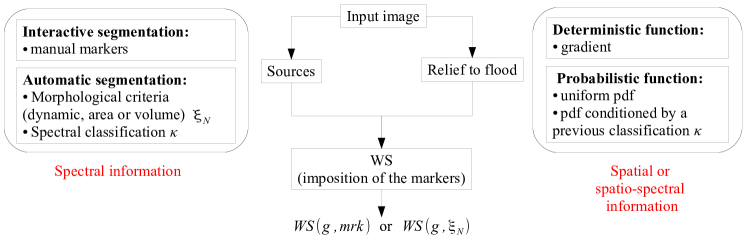
Figure 1: General framework of multispectral image segmentation

Let us start by presenting a general paradigm of WS-based segmentation of multispectral images (fig. 1). This segmentation requires two basic ingredients:

1. some markers for the regions of interest $mrk$;

2. a relief to flood which describes the “energy” of the frontiers between the regions $g$.

The markers can be chosen interactively by a user or automatically by means of a morphological criteria $\xi_{N}$, or with the classes of a previous spectral classification. The relief to flood is a scalar function (i.e., a greyscale image). For the deterministic WS, it is usually a gradient (in fact its norm), or a distance function. For the stochastic WS, the function to flood is a probability density function (pdf) of the contours appearing in the image. After extracting the markers, they are imposed as sources of the relief to flood and the WS is computed. The results are noted $WS(g,mrk)$ or $WS(g,\xi_{N})$.

The segmentation framework for remote sensing images introduced in this paper is coherent with the general paradigm of WS-based segmentation. More precisely, the method is based on classification-driven stochastic watershed by Monte Carlo simulations, and as we will show, it gives more regular and reliable contours than standard watershed.

The approach is decomposed into several sequential steps. Each step was partially considered in our previous works, where our methods were compared with more standard ones. However, the main objective of this paper is to introduce the global pipeline, presenting exclusively for each step the algorithm leading to the best performance.

Firstly in section 3, a dimensionality reduction stage is performed using Factor Correspondence Analysis (FCA) (Benzécri, 1973). In this context, a new way to select the factor axes (i.e. the eigenvectors) according to their spatial information is introduced. Then a spectral classification on the factor space, described in section 5, produces a spectral pre-segmentation of the image. Subsequently, a probability density function (pdf) of contours containing spatial and spectral information is estimated by simulation using a stochastic WS approach driven by the spectral classification. In section 4, the standard stochastic WS is reminded, and then, in section 6, the algorithm for the construction of the classification-driven stochastic WS is discussed. It also includes how the pdf of contours is finally segmented by a watershed controlled by markers coming from a regularization of the initial classification.

The paper is completed with section 2, which fixes the notations used in this paper and which presents the image data considered in the experiments. Finally, in section 7, the conclusions and perspectives of the paper are discussed.

2 Notations

In a formal way, each pixel of a multispectral image is a vector with values in wavelength. To each wavelength corresponds an image in two dimensions called channel. The number of channels depends on the nature of the specific problem under studies (satellite imaging, spectroscopic images, temporal series, etc.). Let

$$\mathbf{f_{\lambda}}:\left\{\begin{array}[c]{lll}E&\rightarrow&\mathcal{T}^{L}\\ x&\rightarrow&\mathbf{f}_{\mathbf{\lambda}}(x)=\left(f_{\lambda_{1}}(x),f_{\lambda_{2}}(x),\ldots,f_{\lambda_{L}}(x)\right)\\ \end{array}\right.$$ (1)

denote an hyperspectral image, where:

1. $E\subset\mathbb{R}^{2}$, $\mathcal{T}\subset\mathbb{R}$ and $\mathcal{T}^{L}=\mathcal{T}\times\mathcal{T}\times\ldots\times\mathcal{T}$

2. $x=x_{i}\ /\ i\in\{1,2,\ldots,P\}$ is the spatial coordinate of a vector pixel $\mathbf{f}_{\lambda}(x_{i})$ ($P$ is the number of pixels of $E$)

3. $f_{\lambda_{j}}\ /\ j\in\{1,2,\ldots,L\}$ is a channel ($L$ is the number of channels)

4. $f_{\lambda_{j}}(x_{i})$ is the value of vector pixel $\mathbf{f}_{\lambda}(x_{i})$ on channel $f_{\lambda_{j}}$.

Figure 2 gives an example of a five band satellite simulated image PLEIADES, acquired by the CNES (Centre National d’Etudes Spatiales, the French space agency) and provided by Flouzat et al. (1998). Its channels are the following: $f_{\lambda_{1}}$ blue, $f_{\lambda_{2}}$ green, $f_{\lambda_{3}}$ red, $f_{\lambda_{4}}$ near infrared and $f_{\lambda_{5}}$ panchromatic. The panchromatic channel, initially $1460\times 1460$ pixels with a resolution of 0.70 meters, was resized to $365\times 365$ pixels. Therefore, the resolution is 2.80 meters in an image of $365\times 365\times 5$ pixels. In order to represent a multispectral image in a synthetic way, we created a synthetic RGB image using channels $f_{\lambda_{3}}$ red, $f_{\lambda_{2}}$ green and $f_{\lambda_{1}}$ blue.

The downsampling method consists in, by averaging, keeping only one pixel on four pixels in both directions of the plane. The coordinates $(i,j)$ of the pixels are ordered as the standard ordering used for matrices. Moreover, we also notice that even if the downsampled panchromatic image has values strongly correlated to average intensity of the red, blue and green channels, the spatial resolution of the panchromatic is better than the chromatic bands, and consequently there is a better resolution of the contours which is important for the aim of image segmentation. Indeed, to deal with the redundancy, the FCA (Factor Correspondence Analysis) transforms the original channels into uncorrelated factor channels (according to the chi-squared metric).

(a) $\mathbf{f}_{\lambda_{1}}$	(b) $\mathbf{f}_{\lambda_{2}}$	(c) $\mathbf{f}_{\lambda_{3}}$
(d) $\mathbf{f}_{\lambda_{4}}$	(e) $\mathbf{f}_{\lambda_{5}}$	(f) RGB

Figure 2: Channels of multispectral image $\mathbf{f}_{\mathbf{\lambda}}$ “Roujan” (©CNES): (a) $\mathbf{f}_{\lambda_{1}}$ blue, (b) $\mathbf{f}_{\lambda_{2}}$ green, (c) $\mathbf{f}_{\lambda_{3}}$ red, (d) $\mathbf{f}_{\lambda_{4}}$ near infra-red, (e) $\mathbf{f}_{\lambda_{5}}$ panchromatic, (f) synthetic RGB representation.

3 Dimensionality reduction

As the number of channels, in a multispectral image, is usually important, the spectrum information contained in these channels is redundant. Therefore, in order to avoid the Hughes phenomenon (Hughes, 1968; Landgrebe, 2002) associated to the spectral dimensionality problem as well as to reduce the computational time, it is necessary to reduce the number of channels.

Consequently, a data reduction is performed using Factor Correspondence Analysis (FCA) Benzécri (1973). We prefer using a FCA instead of a Principal Component Analysis (PCA) or a Maximum Noise Fraction (MNF) (Green et al., 1988), because image values are positive and the spectral channels can be considered as probability distributions.

Green et al. 1988 have demonstrated that PCA and MNF are equivalent in the case of an uncorrelated noise with equal variance in all channels. This explains why PCA is often used to remove noise on hyperspectral images in which the noise is almost uncorrelated with the same variance on all channels.

As for PCA, from selected factorial FCA axes the image can be partially reconstructed. The metric used in FCA is the chi-squared, which is adapted to probability laws and normalized by channels weights. FCA can be seen as a transformation going from image space to a factorial space. In the factorial space, the coordinates of the pixel vector, on each factorial axis, are called pixel factors. The pixel factors can be considered as another multispectral image whose channels correspond to the factorial axes:

$$\zeta:\left\{\begin{array}[c]{lll}\mathcal{T}^{L}&\rightarrow&\mathcal{T}^{K}\text{ / }K<L\\ \mathbf{f}_{\mathbf{\lambda}}(x)&\rightarrow&\mathbf{c}^{\mathbf{f}}_{\alpha}(x)=\left(c^{\mathbf{f}}_{\alpha_{1}}(x),\ldots,c^{\mathbf{f}}_{\alpha_{K}}(x)\right)\\ \end{array}\right.$$ (2)

A limited number $K$, with $K<L$, of factorial axes is usually chosen. Therefore FCA can be seen as a projection of the initial vector pixels in a factor space with a lower dimension. Moreover, as for PCA, FCA reduces the spectral noise on multispectral images (Green et al., 1988; Noyel et al., 2007a; Noyel, 2008). Figure 3 shows FCA factor pixels $\mathbf{c}_{\alpha}^{\mathbf{f}}$ of image “Roujan”. Consequently, we have two spaces for multivariate segmentation: the multispectral image space (MIS) and the factor image space (FIS).

(a) $c^{\mathbf{f}}_{\alpha_{1}}$	(b) $c^{\mathbf{f}}_{\alpha_{2}}$
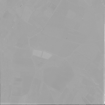
(c) $c^{\mathbf{f}}_{\alpha_{3}}$	(d) $c^{\mathbf{f}}_{\alpha_{4}}$

Figure 3: FCA factors pixels $\mathbf{c}^{\mathbf{f}}_{\alpha}$ of image “Roujan” on axes (a) 1, (b) 2, (c) 3 and (d) 4 with respective inertias 84.1 %, 8.7 %, 6.2 %, 1 %.

A common problem in remote sensing application is the registering of the various spectral images. If the registering step is not perfect, the spatial shifts introduce in the dimensionality reduction a FCA factor containing this information; see for instance, in figure 3, the FCA factor image $c_{\alpha_{2}}^{\mathbf{f}}$. This image looks like a laplacian image, but for the purpose of segmentation, it should be considered as a factor image containing spatial noise. We only show below how to detect and remove these “noisy” factor images.

Another approach to reduce the number of channels consists in modelling the spectrum of each vector-pixel $\mathbf{f}_{\lambda}(x_{i})$ and creating a new multispectral image composed of the parameters of the model (Noyel et al., 2007a); however, for generic multispectral remote sensing images, this kind of modelling is quite difficult.

As shown by Benzécri (1973) and by Green et al. (1988), some factor pixels on factor axes contain mainly noise, and others signal information. In order to select relevant axes containing information (i.e. signal against noise), we introduce a new method based on a measurement of the signal to noise ratio $SNR$ of every factor image. For each factorial axis $\alpha_{k}$, the centered spatial covariance is computed by a 2D FFT (Fast Fourier Transform) on the pixel factors:

$$\overline{g}_{\alpha_{k}}(h)=E[\overline{c}_{\alpha_{k}}^{\mathbf{f}}(x)\overline{c}_{\alpha_{k}}^{\mathbf{f}}(x+h)],$$

with $\overline{c}_{\alpha_{k}}^{\mathbf{f}}(x)=c_{\alpha_{k}}^{\mathbf{f}}(x)-E[c_{\alpha_{k}}^{\mathbf{f}}(x)]$, where $E$ is the mathematical expectation (here the statistical expectation).

The covariance peak, at the origin, contains the sum of the signal variance and the noise variance of the image. Then, the signal variance is estimated by the maximum (i.e. value at the origin) of the covariance $\overline{g}$. Based on the property of the morphological opening which removes intensity peaks smaller than the used structuring element, we apply a morphological opening $\gamma$ on the covariance image with a unitary centered structuring element (square of $3\times 3$ pixels) in order to remove the peak of signal associated to the noise variance: $Var(signal)=\gamma\overline{g}_{\alpha_{k}}(0)$. The noise variance is therefore given by the residue of the opening of the covariance at the origin: $Var(noise)=\overline{g}_{\alpha_{k}}(0)-\gamma\overline{g}_{\alpha_{k}}(0)$ (fig. 4). Hence, the signal to noise ratio is defined for a factor axis $\alpha_{k}$ as:

$$SNR_{\alpha_{k}}=\frac{Var(signal)}{Var(noise)}=\frac{\gamma\overline{g}_{\alpha_{k}}(0)}{\overline{g}_{\alpha_{k}}(0)-\gamma\overline{g}_{\alpha_{k}}(0)}$$ (3)

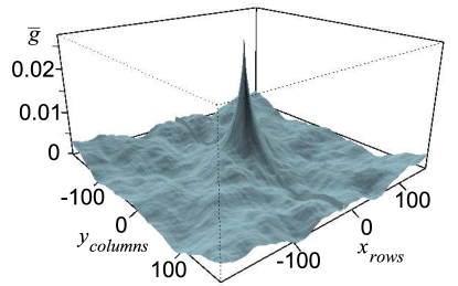
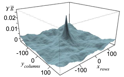
$\overline{g}_{\alpha_{1}}(h)$	$\gamma\overline{g}_{\alpha_{1}}(h)$
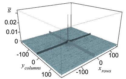
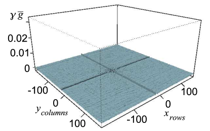
$\overline{g}_{\alpha_{2}}(h)$	$\gamma\overline{g}_{\alpha_{2}}(h)$

Figure 4: 2D covariances for factor pixels $c^{\mathbf{f}}_{\alpha_{1}}$ and $c^{\mathbf{f}}_{\alpha_{2}}$ of image “Roujan” before (left) and after opening (right).

In the current example, by analysis of the factor pixels and their signal to noise ratios, we observe that they are higher for axes 1, $c_{\alpha_{1}}^{\mathbf{f}}$, and 3, $c_{\alpha_{3}}^{\mathbf{f}}$, than for axes 2, $c_{\alpha_{2}}^{\mathbf{f}}$, and 4, $c_{\alpha_{4}}^{\mathbf{f}}$. Therefore, the axes 1 and 3 are retained. For an automatic selection of factor axes, the axes with a SNR lower than 1 are rejected.

In figure 5, we notice that axis 3, which is selected, has a lower inertia than axis 2, which is rejected. Therefore, SNR analysis makes it possible to describe relevant signal in dimensionality reduction, more than inertia-like criterion.

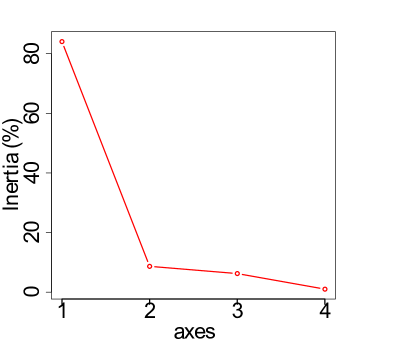
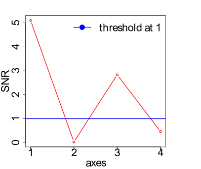
Figure 5: Inertia (%) and SNR for factor pixels of image “Roujan”.

4 Introduction to stochastic WS

Angulo and Jeulin (2007) defined a new method of stochastic WS for greyscale and color images. This method was extended to hyperspectral images by Noyel et al. (2007c). In addition, the segmentation of multispectral images by classical (deterministic) WS was presented in (Noyel et al., 2007a). Several improvements were made by Noyel et al. (2008a); Noyel (2008).

4.1 Principle of the stochastic WS

One of the main artefacts of the classical watershed is that small regions strongly depend on the position of the markers, or on the volume (i.e. the integral of the grey levels) of the catchment basin, associated to their minima. In fact, there are two kinds of contours associated to the watershed of a gradient: first order contours, which correspond to significant regions and which are relatively independent from markers; second order contours, associated to “small”, “low” contrasted and textured regions, which depend strongly on the location of markers. Stochastic watershed aims at enhancing the first order contours from a sampling effect, to improve the result of the watershed segmentation.

Let us consider $\{mrk_{i}(x)\}_{i=1}^{M}$ a series of $M$ realisations of $N$ uniform or regionalized random germs. Each of these binary images is considered as the marker for a watershed segmentation of a scalar gradient or a vector gradient. Therefore, a series of segmentations is obtained, i.e. $\{sg_{i}^{mrk}(x)\}_{i=1}^{M}$. Starting from the $M$ realisations of contours, the probability density function $pdf(x)$ of contours is computed by the Parzen window method. The kernel density estimation by Parzen window (Duda and Hart, 1973) is a way to estimate the probability density function (pdf) of a random variable. Let $\mathbf{x}_{1},\mathbf{x}_{2},\cdots,\mathbf{x}_{M}\in\mathbb{R}^{n}$ be $M$ samples of a random variable, the kernel density approximation of its pdf is: $\widehat{f}_{h}(\mathbf{x})=\frac{1}{Nh}\sum_{i=1}^{N}K\left(\frac{\mathbf{x}-\mathbf{x}_{i}}{h}\right)$, where $K(\mathbf{x})$ is some kernel and the bandwidth $h$ a smoothing parameter. Usually, $K(\mathbf{x})$ is taken to be a Gaussian function, $G_{\sigma}$, with mean zero and variance $\sigma^{2}$. The smoothing effect of the Gaussian convolution kernel (typically $\sigma=3$ working on contours of one pixel width) is important to obtain a function where near contours, such as textured regions or associated to small regions, are added together. In other words, the WS lines with a very low probability, which correspond to non significant boundaries, are filtered out.

The pdf of contours could be thresholded to obtain the most prominent contours. However, to obtain closed contours, the pdf image can be also segmented, as we consider here, using a watershed segmentation.

4.2 Influence of parameters

The stochastic WS needs two parameters:

1. $M$ realisations of germs. The method is almost independent on $M$ if it is large enough. Practically, the convergence is ensured for $M$ in the range 20 - 50. We propose to use $M$ equal to 100.

2. $N$ germs (or markers): In WS segmentation the number of regions obtained is equal to the number of markers. In the case of the stochastic WS, if $N$ is small, a segmentation in large regions is privileged; if $N$ is too large, the over-segmentation of $sg_{i}^{mrk}$ leads to a very smooth $pdf$, which looses its properties to select the $R$ regions. Therefore, the stochastic WS mainly depends on $N$, but is linked to the number of regions $R$ which should be finally selected. As it was shown in (Angulo and Jeulin, 2007), it is straightforward to use $N>R$.

As it is described below, in section 6, in this study the number of markers of each realization used in the conditioned stochastic WS will be equal to the number of connected classes of the classification $\widehat{\kappa}$ different of the void class.

5 Generation of markers from a classification

To segment the pdf of contours by WS, it is necessary to have markers for the spectral objects of interests. The latter are obtained by a spectral classification. This classification step groups the pixels into classes with similar spectra. In fact, each pixel is compared to all the others, leading to a global comparison of the image spectra. We have tested two kinds of methods for spectral classification on multispectral images: unsupervised methods and supervised methods.

In the case of remote sensing, we show results obtained by an unsupervised method such as “clara” (Kaufman and Rousseeuw, 1990). Unsupervised and supervised methods in remote sensing using mathematical morphology as well as the “clara” method are also investigated in (Epifanio and Soille, 2007). For other contexts different from remote sensing, we tested other unsupervised methods such as k-means and supervised methods such as Linear Discriminant Analysis (Noyel et al., 2008b; Noyel, 2008). One of the strong points of supervised approaches is to integrate prior information about spectrum classes into the classification. However, in generic remote sensing segmentation problems, we are not looking for a special kind of spectrum. Therefore, we prefer, in the presentation of the current paper, to use an unsupervised classification with a unique parameter, namely the number of classes.

Hence, after the data reduction and the spectral filtering stage by FCA, a spectral classification by “clara” is performed on the factor space. We have to stress that a correct classification, used later for constructing the pdf, requires factor pixels without noise. The classification algorithm uses an Euclidean distance which is coherent with the metric of the factor space (Noyel et al., 2007a). The unique parameter is the number of classes, which is chosen in order to get a good separation of  the classes. Here, for this example, 3 classes are retained (fig. 6).

(a) RGB “Roujan”	(b) $\kappa$	(c) $\widehat{\kappa}$
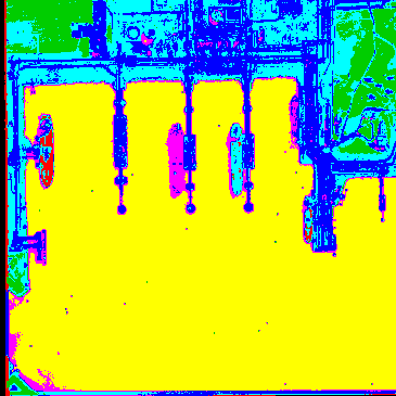
(d) RGB “Port de Bouc”	(e) $\kappa$	(f) $\widehat{\kappa}$

Figure 6: First line: (a) Synthetic RGB image “Roujan”, (b) classification $\kappa$ in 3 classes in factor space formed by $c^{\mathbf{f}}_{\alpha_{1}}$ and $c^{\mathbf{f}}_{\alpha_{3}}$ and (c) transformed classification $\widehat{\kappa}=\Upsilon(\kappa)$. Second line: (d) Synthetic RGB image “Port de Bouc”, (e) classification $\kappa$ in 7 classes in factor space formed by $c^{\mathbf{f}}_{\alpha_{1}}$ and $c^{\mathbf{f}}_{\alpha_{2}}$ and (f) transformed classification $\widehat{\kappa}=\Upsilon(\kappa)$. The void class is in black on the images $\widehat{\kappa}$. The way to compute the transformed classification is explained in section 6.1. The colours correspond to the labels of the transformed classification obtained after a new labellisation.

6 Multispectral segmentation by stochastic watershed

The previously obtained spectral classification of pixels leads to a spatial partition of the image on regions which are spectrally homogeneous. This initial partition is denoted $\kappa$. However, they do not define a partition into spatial connected classes: various connected components belong to the same spectral class. In order to address this issue, a segmentation stage is needed which introduces spatial information (i.e., regional information). In this section, after presenting an algorithm to pre-process the previous classification $\kappa$, the extension of stochastic WS to multispectral images is explained; then we show a way to constrain the pdf by the previous spectral classification.

6.1 Pre-processing of markers coming from  the classification

A pre-processing of the connected classes of the classification is necessary for two reasons:

1. to give necessary degrees of freedom to the final WS of the pdf. Actually, if we use the connected classes of the classification $\kappa$ as markers of the flooding process, then the WS is completely defined by the limit of the classes after labelling them into connected classes. Therefore we propose to process the initial partition using an anti-extensive transformation such as an erosion (Serra, 1982; Soille, 2003). For instance, using a structuring element (SE) of size 5 $\times$ 5 pixels each spatial class is reduced and the smallest classes disappear. We consider that classes corresponding to “noise” are totally removed. The smallest classes could also be removed by means of an area opening (Soille, 2003). Therefore, after processing the initial partition, a partial partition is obtained. There are several alternatives to deal with the problem that the partial partition is not a partition of the support space; for instance adding to the partial partition the singletons outside its support. We prefer however the following solution. We introduce a particular label, the “void class”, in such a way that after processing the initial partition, covering the whole space, a new partition is also obtained. In the new partition, the existing classes are modified (reduced) and in addition, a new class is introduced, the void class. If we want to keep all the classes, for instance if the aim is to segment thin objects as a network of roads, we could use a homotopic thinning instead of an erosion.

2. to fill the holes inside the largest classes with an extensive transformation such as a closing by reconstruction with a SE of size for instance 3 $\times$ 3 pixels (Serra, 1982; Soille, 2003).

The transformations are applied to each class of the initial spectral classification. More precisely to each spectral class, $\kappa(n)$ with $n=1,\ldots,N$, of the previous classification $\kappa=\cup_{n}\kappa(n)$, an index function (i.e. a binary image) is associated:

$$h_{\kappa(n)}(x)=\left\{\begin{array}[c]{lll}1,&\text{if}&x\in\kappa(n);\\ 0,&\text{otherwise.}&\\ \end{array}\right.$$ (4)

Then, the sequence of the anti-extensive and extensive transformations are applied to each index function, $h_{\kappa(n)}$ for all $n=1,\ldots,N$, in order to obtain the transformed index function $h_{\kappa(n)}^{\prime}$. Then the supremum (union) of the index functions is computed, followed by a standard labelling to obtain the connected components which correspond to markers for the segmentation, except for the void class which is not a marker. The complete transform is noted $\Upsilon$, and it results in a new partition $\widehat{\kappa}=\Upsilon(\kappa)$ (fig. 6). The partition $\widehat{\kappa}$ will then be strongly used for the spatial segmentation by stochastic WS.

6.2 Extension of the stochastic WS to multivariate or hyperspectral images

The extension of the stochastic WS was first presented in Noyel et al. (2007c). The key points are recalled in the current paper.

6.2.1 Spectral distances and gradient

In order to segment images according to watershed-based paradigms, a gradient is needed. A gradient image, in fact its norm, is a scalar function with values in the reduced interval $[0,1]$ (after normalisation), i.e. $\varrho(x):E\rightarrow[0,1]$. In order to define a gradient, two approaches are considered: the standard symmetric morphological gradient on each marginal channel and a metric-based vectorial gradient on all channels.

The morphological gradient is defined for scalar images $f$ as the difference between dilation and erosion by a unit structuring element $B$, i.e.,

$$\varrho(f_{\lambda_{j}}(x)) = \delta_{B}(f_{\lambda_{j}}(x))-\varepsilon_{B}(f_{\lambda_{j}}(x))$$

$$= \vee[f_{\lambda_{j}}(y),y\in B(x)]-\wedge[f_{\lambda_{j}}(y),y\in B(x)]\text{ .}$$

As it was shown in Hanbury and Serra (2001), the morphological gradient can be generalised to vectorial image by using the following relation:

$$\{f(x)-\vee[f(y),y\in B(x),y\neq x]\}=\wedge\{f(x)-f(y),y\in B(x),y\neq x\}$$

and the relation obtained by the inversion of the suprema and infima. The morphological gradient can be written in a form that is only composed of increments computed in the neighborhood $B$ centered at point $x$:

$$\varrho(f)(x)=\vee[f(x)-f(y),y\in B(x),y\neq x]-\wedge[f(x)-f(y),y\in B(x),y\neq x]\text{ .}$$

To extend this relation to multivariate functions, it is sufficient to replace the increment $[f(x)-f(y)]$ by a distance between vector pixels $d(\mathbf{f_{\lambda}}(x),\mathbf{f_{\lambda}}(y))$ to obtain the following metric-based gradient:

$$\varrho_{d}\mathbf{f_{\lambda}}(x)=\vee[d(\mathbf{f_{\lambda}}(x),\mathbf{f_{\lambda}}(y)),y\in B(x),y\neq x]-\wedge[d(\mathbf{f_{\lambda}}(x),\mathbf{f_{\lambda}}(y)),y\in B(x),y\neq x]\text{ .}$$

Various metric distances, useful for multispectral images, are available for this gradient such as:

• the Euclidean distance:

  $$d_{E}(\mathbf{f_{\lambda}}(x),\mathbf{f_{\lambda}}(y))=\sqrt{\sum_{j=1}^{L}(f_{\lambda_{j}}(x)-f_{\lambda_{j}}(y))^{2}},$$

  and

• the Chi-squared distance:

  $$d_{\chi^{2}}(\mathbf{f}_{\lambda}(x_{i}),\mathbf{f}_{\lambda}(x_{i^{\prime}}))=\sqrt{\sum_{j=1}^{L}\frac{S}{f_{.\lambda_{j}}}\left(\frac{f_{\lambda_{j}}(x_{i})}{f_{x_{i}.}}-\frac{f_{\lambda_{j}}(x_{i^{\prime}})}{f_{x_{i^{\prime}}.}}\right)^{2}}$$

  with $f_{.\lambda_{j}}=\sum_{i=1}^{P}f_{\lambda_{j}}(x_{i})$, $f_{x_{i}.}=\sum_{j=1}^{L}f_{\lambda_{j}}(x_{i})$ and $S=\sum_{j=1}^{L}\sum_{i=1}^{P}f_{\lambda_{j}}(x_{i})$.

An important point is to choose an appropriate distance depending on the space used for image representation: Chi-squared distance is adapted to MIS and Euclidean distance to FIS. More details on multivariate gradients are given by Noyel et al. (2007a). Another example of a multivariate gradient is given by Scheunders (2002).

6.2.2 Probability density function for multispectral images

We studied two ways to extend the pdf  gradient to multispectral images:

1. the first one is a marginal approach (i.e. channel by channel) called marginal pdf $mpdf$ (alg. 1 and fig. 7)

2. the second one is a vectorial approach (i.e. vector pixel by vector pixel) called vectorial pdf $vpdf$ (alg. 2 and fig. 8).

Algorithm 1 $mpdf$

1:  For the morphological gradient of each channel $\varrho(f_{\lambda_{j}})$, $j\in[1,\ldots,L]$, throw $M$ realisations of $N$ uniform random germs, i.e. the markers $\{mrk^{j}_{i}\}_{i=1\ldots M}^{j=1\ldots L}$, generating $M\times L$ realisations. Get the series of segmentations, $\{sg^{j}_{i}(x)\}_{i=1\ldots M}^{j=1\ldots L}$, by watershed associated to morphological gradients of each channel $\varrho(f_{\lambda_{j}})$.

2:  Get the marginal pdfs on each channel by Parzen method: $pdf_{j}(x)=\frac{1}{M}\sum_{i=1}^{M}sg^{j}_{i}(x)\ast G_{\sigma}$.

3:  Obtain the weighted marginal pdf:

$$mpdf(x)=\sum_{j=1}^{L}w_{j}pdf_{j}(x)$$ (5)

with $w_{j}=1/L$, $j\in[1,\ldots,L]$ in MIS and $w_{j}$ equal to the inertia axes in FIS.

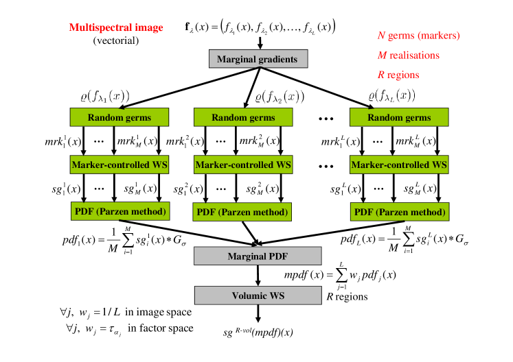
Figure 7: General framework stochastic WS on marginal pdf $mpdf$ for multispectral images

Algorithm 2 $vpdf$

1:  For the vectorial gradient $\varrho^{d}(\mathbf{f_{\lambda}})$, throw $M\times L$ realisations of $N$ uniform random germs, i.e. the markers $\{mrk_{i}\}_{i=1\ldots M\times L}$, with $L$ the channels number. Get the segmentation, $\{sg_{i}(x)\}_{i=1\ldots M\times L}$, by watershed associated to the vectorial gradient $\varrho^{d}(\mathbf{f_{\lambda}})$, with $d=d_{\chi^{2}}$ in MIS or $d=d_{E}$ in FIS.

2:  Obtain the probability density function:

$$vpdf(x)=\frac{1}{M\times L}\sum_{i=1}^{M\times L}sg_{i}(x)\ast G_{\sigma}\text{ .}$$ (6)

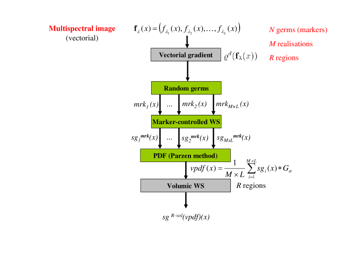
Figure 8: General framework stochastic WS on vectorial pdf $vpdf$ for multispectral images

The probabilistic gradient was also defined in (Angulo and Jeulin, 2007) to ponder the enhancement of the largest regions by the introduction of smallest regions. It is defined as $\varrho_{prob}=mpdf+\varrho^{d}$: after normalization in $[0,1]$ of the weighted marginal pdf $mpdf$ and the metric-based gradient $\varrho^{d}$.

In order to obtain a partition from the $mpdf$, $vpdf$ or the gradient $\varrho_{prob}$, these probabilistic functions can be segmented for instance by a hierarchical WS with a volume criterion (see the examples of fig. 9), as studied in Noyel et al. (2007c). In such a case, the goal is not to find all the regions. In fact, the stochastic WS addresses the problem of segmentation of an image in few pertinent regions, according to a combined criterion of contrast and size. In the present study, as we discuss below, the segmentation of the pdf is obtained from markers of the processed classification. In Noyel et al. (2007c) was also shown that marginal pdf and vectorial pdf give similar results in multispectral image space (MIS) and in factor image space (FIS), as we can also observe in comparison of fig. 9. Consequently, in what follows, we choose to work on the MIS to show that our method is not limited by the number of channels.

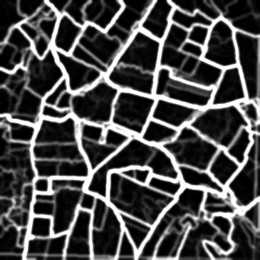
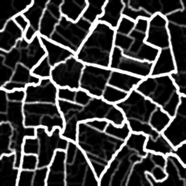
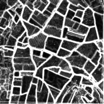
(a) $\varrho^{\chi^{2}}(\mathbf{f_{\lambda}})$	(b) $mpdf(\mathbf{f_{\lambda}})$	(c) $vpdf(\mathbf{f_{\lambda}})$	(d) $\varrho_{prob}(\mathbf{f_{\lambda}})$
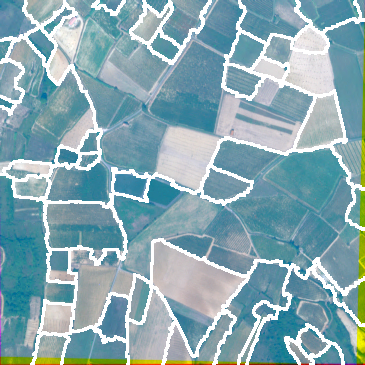
(e) $seg^{vol}(\varrho^{\chi^{2}}(\mathbf{f}_{\lambda}),R)$	(f) $seg^{vol}(mpdf(\mathbf{f}_{\lambda}),R)$	(g) $seg^{vol}(vpdf(\mathbf{f}_{\lambda}),R)$	(h) $seg^{vol}(\varrho_{prob}(\mathbf{f}_{\lambda}),R)$

Figure 9: Top: (a) Gradients and (b, c, d) pdf; bottom: (e, f, g, h) associated WS segmentations, with a volume criterion, on image “Roujan”, in MIS, with $N=50$ points , $M=100$ realisations, $R=50$ regions with the largest volume.

6.3 Conditioning the germs of the pdf by a previous classification

The pdf of contours with uniform random germs is constructed without any prior information about the spatial/spectral distribution of the image. In this part, we introduce spectral information by conditioning the germs by the previous transformed classification $\widehat{\kappa}$. Therefore this obtained pdf contains spatio-spectral information. It is possible to use point germs or random ball germs whose location is conditioned by the classification. An exhaustive study is presented by Noyel (2008); Noyel et al. (2008c). In the sequel we present random ball germs regionalized by a classification where each connected class may be hit one time, $mrk_{i}^{\kappa-b}(x)$.

Let us explain the procedure. The transformed classification $\widehat{\kappa}$ is composed of connected classes, $\widehat{\kappa}=\cup_{k}C_{k}$ with $C_{k}\cap C_{k^{\prime}}=\emptyset$, for $k\neq k^{\prime}$. The void class is written $C_{0}$. Then the random germs are drawn conditionally to the connected components $C_{k}$ of the filtered classification $\widehat{\kappa}$. To do this, the following rejection method is used: the random point germs are uniformly distributed. If a point germ $m$ falls inside a connected component $C_{k}$ of minimal area $S$ and not yet marked, then it is kept, otherwise it is rejected. Therefore not all the germs are kept. These point germs are called random point germs regionalized by the classification $\kappa$. However, the regionalized point germs are sampling all the classes independently of their prior estimate of class size/shape, given by the classification. In order to tackle with this limitation, we propose to use random balls as germs.

The centers of the balls are the random point germs and the radii $r$ are uniformly distributed between $0$ and a maximum radius $Rmax$: $\mathcal{U}[1,Rmax]$. Only the intersection between the ball $B(m,r)$ and the connected component $C_{p}$ is kept as a germ. These balls are called random balls germs regionalized by the classification $\kappa$ and noted $mrk_{i}^{\kappa-b}(x)$.

The algorithm 3 sketches the process. We notice that $N$ is the number of random germs to be generated. The effective number of implanted germs is less than $N$.

Algorithm 3 Random ball germs regionalized by a classification (each connected class may be hit one time) $mrk_{i}^{\kappa-b}(x)$

1:  Given $N$ the number of drawn germs $m$

2:  Set the background class and the void class $C_{0}$ to marked

3:  for all  drawn germs $m$ from 1 to $N$  do

4:        if $C_{k}$, such as $m\in C_{k}$, is not marked then

5:              $r=\mathcal{U}[1,Rmax]$

6:              Keep as a germ $\mathrm{B}(m,r)\cap C_{k}$

7:              Set the class $C_{k}$ to marked

8:        end if

9:  end for

We use the marginal pdf to show our results. Some random ball germs regionalized by a classification, $\{mrk_{i}^{\kappa-b,j}(x)\}_{i=1\ldots 5}^{j=1}$, their associated realisations of contours, $\{sg_{i}^{j}(x)\}_{i=1\ldots 5}^{j=1}$, and the marginal pdf computed in MIS, $mpdf^{\kappa-b}(\mathbf{f}_{\lambda})$, are presented in figure 10.

A comparison between the marginal pdf with uniform random point germs, $mpdf^{pt}(\mathbf{f}_{\lambda})$ (noted before $mpdf(\mathbf{f}_{\lambda})$) and the marginal pdf with random ball germs $mpdf^{\kappa-b}(\mathbf{f}_{\lambda})$ is shown in figure 11. These pdf are segmented by hierarchical WS with a volume criterion, $sg^{R-vol}(mpdf^{pt}(\mathbf{f}_{\lambda}))$ and $sg^{R-vol}(mpdf^{\kappa-b}(\mathbf{f}_{\lambda}))$. In this particular example, the advantage of the pdf obtained with the conditioned random balls is obvious with respect to the pdf from uniform random point germs. Moreover, in order to compare the results of segmentation of example of figure 11, we must notice that in both images only the $8$ most important regions have been segmented. If the purpose is to segment all the objects, including the smallest ones, we only need to increase the number of desired volumic regions.

i = 1	i = 2	i = 3	i = 4	i = 5
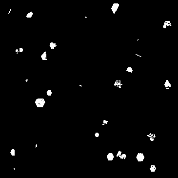
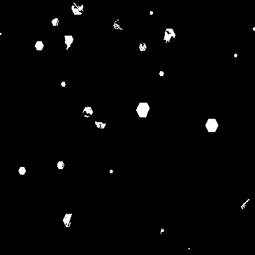
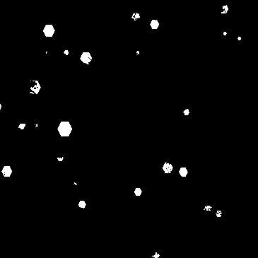
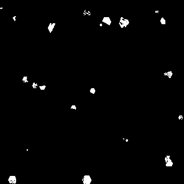
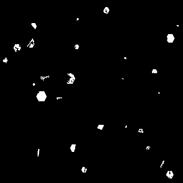
(a) $mrk_{1}^{\kappa-b,1}(x)$	(b) $mrk_{2}^{\kappa-b,1}(x)$	(c) $mrk_{3}^{\kappa-b,1}(x)$	(d) $mrk_{4}^{\kappa-b,1}(x)$	(e) $mrk_{5}^{\kappa-b,1}(x)$
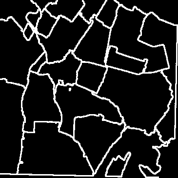
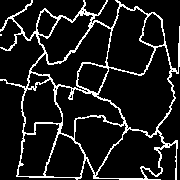
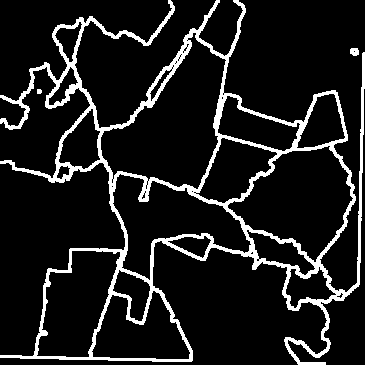
(f) $sg_{1}^{1}(x)$	(g) $sg_{2}^{1}(x)$	(h) $sg_{3}^{1}(x)$	(i) $sg_{4}^{1}(x)$	(j) $sg_{5}^{1}(x)$
		(k) $mpdf^{\kappa-b}(\mathbf{f}_{\lambda})$

Figure 10: (a, b, c, d, e) A few realisations of regionalized random ball germs $\{mrk_{i}^{\kappa-b,j}(x)\}_{i=1\ldots 5}^{j=1}$ (top) by the classification $\kappa$ and (f, g, h, i, j) associated contours of watershed $\{sg_{i}^{j}(x)\}_{i=1\ldots 5}^{j=1}$ (bottom). $i$ is the index of realisations and $j$ the number of the considered channel. The parameters are the maximum radius $Rmax$ = 30 pixels and the maximum number of germs $N$ = 50. (k) The marginal pdf with regionalized random ball germs $mpdf^{\kappa-b}(\mathbf{f}_{\lambda})$ is computed with $M=100$ realisations.

(a) $mpdf^{pt}(\mathbf{f}_{\lambda})$	(b) $sg^{R-vol}(mpdf^{pt}(\mathbf{f}_{\lambda}))$
(c) $mpdf^{\kappa-b}(\mathbf{f}_{\lambda})$	(d) $sg^{R-vol}(mpdf^{\kappa-b}(\mathbf{f}_{\lambda}))$

Figure 11: Comparison between (a) the pdf $mpdf^{pt}(\mathbf{f}_{\lambda})$ and (b) the associated stochastic WS with uniform random point germs with a volume criterion $sg^{R-vol}(mpdf^{pt}(\mathbf{f}_{\lambda}))$ to (c) the pdf $mpdf^{\kappa-b}(\mathbf{f}_{\lambda})$ and (d) the associated stochastic WS with regionalized random ball germs with a volume criterion $sg^{R-vol}(mpdf^{\kappa-b}(\mathbf{f}_{\lambda}))$. Only $R=8$ regions with the largest volume are retained. For visualization, the contours of the segmentations are dilated by a SE of size $3\times 3$ pixels.

6.4 Segmentation of the pdf

After having built the pdf, a segmentation stage is required to obtain the contours of the image. Two possibilities were tested:

1. a marker-controlled WS using as markers the transformed classification $sg^{mrk}(mpdf^{\kappa-b}(\mathbf{f}_{\lambda}),\widehat{\kappa})$ (Noyel et al., 2008a). In this case, no more parameter is required.

2. a hierarchical WS with a volume criterion $sg^{R-vol}(mpdf^{\kappa-b}(\mathbf{f}_{\lambda}))$ (Noyel et al., 2007c). Therefore, it is necessary to define an additional parameter: the number of regions with the largest volume.

In order to show the robustness of our approach we used the same method to build the pdf conditioned by the classification on similar images “Roujan”, “Roujan 0 2” and “Roujan 0 9”. As for image “Roujan”, factor axes $c^{\mathbf{f}}_{\alpha_{1}}$ and $c^{\mathbf{f}}_{\alpha_{3}}$ are kept because th Signal to Noise Ratio (SNR) is less than thresholded value (1). Inertias and SNR for factor axes of images “Roujan X X” are presented in the tables 6.4 and 6.4.

Part of inertia for factor axes of images “Roujan X X” Image $c^{\mathbf{f}}_{\alpha_{1}}$ $c^{\mathbf{f}}_{\alpha_{2}}$ $c^{\mathbf{f}}_{\alpha_{3}}$ $c^{\mathbf{f}}_{\alpha_{4}}$ “Roujan” 84.1 % 8.7 % 6.2 % 1 % “Roujan 0 2” 75.6 % 13.7 % 9.2 % 1.5 % “Roujan 1 9” 77.5 % 12.1 % 9 % 1.4 %

SNR for factor axes of images “Roujan X X” Image $c^{\mathbf{f}}_{\alpha_{1}}$ $c^{\mathbf{f}}_{\alpha_{2}}$ $c^{\mathbf{f}}_{\alpha_{3}}$ $c^{\mathbf{f}}_{\alpha_{4}}$ “Roujan” 5.10 0.03 2.84 0.47 “Roujan 0 2” 2.66 0.01 2.53 0.32 “Roujan 1 9” 3.15 0 2.90 0.51

A classification “clara” is made on the factor pixels of these two axes. The marginal pdf, $mpdf^{\kappa-b}(\mathbf{f}_{\lambda})$, is produced as explained for image “Roujan”.

The parameters for the stochastic WS controlled by markers $sg^{mrk}(mpdf^{\kappa-b}(\mathbf{f}_{\lambda}),\widehat{\kappa})$ are:

• the number of classes for the classification $\kappa$: $Q=3$. It is the only important parameter;

• the maximum number of random ball germs: $N=50$, which must be high enough and which must be of the the same order as the number of regions in the image;

• the number of realisations for each channel: $M=100$, which always has the same value;

• the minimum area $S=10$ pixels for the connected classes of the classification, generally the same;

• the parameters for pre-processing the initial spectral classification are an erosion using a $5\times 5$ square and a closing by reconstruction using as marker a dilation using a $3\times 3$ square, generally the same;

• the maximum radius of the random ball $Rmax=30$, generally the same.

The final segmentations with marker-controlled WS, $sg^{mrk}(mpdf^{\kappa-b}(\mathbf{f}_{\lambda}),\widehat{\kappa})$, and hierarchical WS with a volume criterion, $sg^{R-vol}(mpdf^{\kappa-b}(\mathbf{f}_{\lambda}))$, are shown on figure 12. We notice that the number of regions, resulting from the segmentation, strongly depends on the image, whereas the number of spectral classes is the same for similar images. In fact, the number of regions for volumic WS, $sg^{vol}$, must be chosen according to the spatial diversity of the considered image, and cannot be easily fixed “a priori” (50 here). The number of regions depends on the size and the complexity of the image, while the number of spectral classes depends on the spectral content, which for a specific domain can be relatively constant. Consequently, it is more relevant to segment the pdf with markers coming also from the classification $sg^{mrk}$. Indeed, only one parameter is needed for marker-controlled WS $sg^{mrk}(mpdf^{\kappa-b}(\mathbf{f}_{\lambda}),\widehat{\kappa})$: the number of classes $Q$ in the classification $\kappa$. Moreover, in that sense, the approach based on the number of classes $Q$ produces a more robust segmentation than the approach based on the number of regions $R$.

Roujan
	(a) $\widehat{\kappa}$	(b) $sg^{mrk}(mpdf^{\kappa-b}(\mathbf{f}_{\lambda}),\widehat{\kappa})$	(c) $sg^{R-vol}(mpdf^{\kappa-b}(\mathbf{f}_{\lambda}))$
		140 regions	50 regions
Roujan 0 2
	(d) $\widehat{\kappa}$	(e) $sg^{mrk}(mpdf^{\kappa-b}(\mathbf{f}_{\lambda}),\widehat{\kappa})$	(f) $sg^{R-vol}(mpdf^{\kappa-b}(\mathbf{f}_{\lambda}))$
		162 regions	50 regions
Roujan 1 9
	(g) $\widehat{\kappa}$	(h) $sg^{mrk}(mpdf^{\kappa-b}(\mathbf{f}_{\lambda}),\widehat{\kappa})$	(i) $sg^{R-vol}(mpdf^{\kappa-b}(\mathbf{f}_{\lambda}))$
		142 regions	50 regions

Figure 12: Comparison between segmentations $sg^{mrk}(mpdf^{\kappa-b}(\mathbf{f}_{\lambda}),\widehat{\kappa})$ (b, e, h) with markers coming from the filtered classification $\widehat{\kappa}$ (a, d, g) and segmentations $sg^{R-vol}(mpdf^{\kappa-b}(\mathbf{f}_{\lambda}))$ (c, f, i) by stochastic WS with a prior given number of regions $R=50$. The results are given for images: “Roujan”, “Roujan 0 2”, “Roujan 1 9”.

In order to show that the stochastic WS, conditioned by a previous classification, produces contours which are more regular and robust than deterministic (standard) WS, we compare the results of a deterministic approach to a stochastic one:

1. For both cases, an unsupervised classification $\kappa$ (“clara”) is processed in factor space FIS and transformed $\widehat{\kappa}=\Upsilon(\kappa)$.

2. • For the deterministic approach, a chi-squared metric based gradient $\varrho^{\chi^{2}}(\mathbf{f}_{\lambda})$ is computed in image space MIS, as a function to flood.

   • For the stochastic approach, a marginal probability density function $mpdf^{\kappa-b}(\mathbf{f}_{\lambda})$, with regionalized random ball germs conditioned by the classification $\kappa$, is processed, in image space MIS, as a function to flood.

3. In both cases, the flooding function is segmented by a watershed (WS) using as sources of flooding the markers from the transformed classification $\widehat{\kappa}$.

The parameters for the stochastic WS controlled by markers are the same as in part 6.4. In figure 13, are given the results of segmentation by deterministic and stochastic WS for image “Roujan” with markers coming from the transformed classification $\widehat{\kappa}$. We observe that the contours are smoother and follow more precisely the main limits of the regions for the stochastic approach than for the deterministic one. The same observation is made on the image “Port de Bouc” classified in $Q=7$ classes. (fig. 14).

(a) $\kappa$ (b) $\widehat{\kappa}$

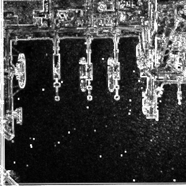
(c) $\varrho^{\chi^{2}}(\mathbf{f}_{\lambda})$ (d) $sg^{mrk}(\varrho^{\chi^{2}}(\mathbf{f}_{\lambda}),\widehat{\kappa})$ (e) zoom $sg^{mrk}(\varrho^{\chi^{2}}(\mathbf{f}_{\lambda}),\widehat{\kappa})$ (f) $mpdf^{\kappa-b}(\mathbf{f}_{\lambda})$ (g) $sg^{mrk}(mpdf^{\kappa-b}(\mathbf{f}_{\lambda}),\widehat{\kappa})$ (h) zoom $sg^{mrk}(mpdf^{\kappa-b}(\mathbf{f}_{\lambda}),\widehat{\kappa})$

Figure 13: (First line) (a) Classification in 3 classes $\kappa$ and (b) markers coming from the classification $\widehat{\kappa}$ on image “Roujan”. (Second line) (d, e) deterministic approach $sg^{mrk}(\varrho^{\chi^{2}}(\mathbf{f}_{\lambda}),\widehat{\kappa})$ on (c) the chi-squared metric based gradient $\varrho^{\chi^{2}}(\mathbf{f}_{\lambda})$. (Third line) (g, h) Stochastic approach $sg^{mrk}(mpdf^{\kappa-b}(\mathbf{f}_{\lambda}),\widehat{\kappa})$ on (f) the marginal pdf $mpdf^{\kappa-b}(\mathbf{f}_{\lambda})$. The parameters are $Q=3$ classes, $N=50$ germs $M=100$ realisations, minimal area $S=10$ pixels, maximum radius $Rmax=30$ pixels). For presentation of images without zoom, the contours are dilated by a SE $3\times 3$ pixels.

(a) $\kappa$	(b) $\widehat{\kappa}$

(c) $\varrho^{\chi^{2}}(\mathbf{f}_{\lambda})$	(d) $sg^{mrk}(\varrho^{\chi^{2}}(\mathbf{f}_{\lambda}),\widehat{\kappa})$	(e) zoom $sg^{mrk}(\varrho^{\chi^{2}}(\mathbf{f}_{\lambda}),\widehat{\kappa})$
(f) $mpdf^{\kappa-b}(\mathbf{f}_{\lambda})$	(g) $sg^{mrk}(mpdf^{\kappa-b}(\mathbf{f}_{\lambda}),\widehat{\kappa})$	(h) zoom $sg^{mrk}(mpdf^{\kappa-b}(\mathbf{f}_{\lambda}),\widehat{\kappa})$

Figure 14: First line) (a) Classification in 3 classes $\kappa$ and (b) markers coming from the classification $\widehat{\kappa}$ on image “Port de Bouc”. (Second line) (d, e) deterministic approach $sg^{mrk}(\varrho^{\chi^{2}}(\mathbf{f}_{\lambda}),\widehat{\kappa})$ on (c) the chi-squared metric based gradient $\varrho^{\chi^{2}}(\mathbf{f}_{\lambda})$. (Third line) (g, h) Stochastic approach $sg^{mrk}(mpdf^{\kappa-b}(\mathbf{f}_{\lambda}),\widehat{\kappa})$ on (f) the marginal pdf $mpdf^{\kappa-b}(\mathbf{f}_{\lambda})$. The parameters are $Q=7$ classes, $N=50$ germs $M=100$ realisations, minimal area $S=10$ pixels, maximum radius $Rmax=30$ pixels). For presentation of images without zoom, the contours are dilated by a SE $3\times 3$ pixels.

6.5 General method of multispectral segmentation by stochastic WS

After all these observations and analysis, we can summarize now the algorithmic pipeline of the general method of segmentation of multispectral image by stochastic WS. The framework is presented on figure 15. The different steps are as follows:

• a FCA to reduce the spectral dimension of the image $\mathbf{f}_{\lambda}$ and eventually to filter the noise. This transformation creates a factor image $\mathbf{c}^{\mathbf{f}}_{\alpha}$

• the previous step requires the selection of factorial axes by the signal to noise ratio (SNR) of the factor pixels

• a spectral classification to group pixels into homogeneous classes (global point-wise comparison)

• a morphological transform $\Upsilon$ of each classes. The image transformed is noted $\widehat{\kappa}=\Upsilon(\kappa)$

• the building of a pdf of contours that can be marginal $mpdf$ or vectorial $vpdf$ starting from a gradient on the image space $\mathbf{f}_{\lambda}$ (MIS) or factor space $\mathbf{c}_{\alpha}^{\mathbf{f}}$ (FIS) with random-balls germs regionalized by the spectral classification

• a segmentation of the pdf by a WS controlled by markers coming from the classes of the transformed classification $\widehat{\kappa}$

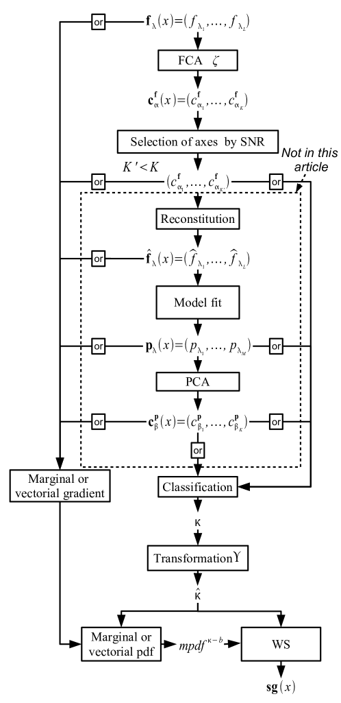
Figure 15: General framework of WS controlled by a classification, with regionalized random-balls germs. The part outlined with a dotted line is not presented in this paper.

Some of the steps presented in the flowchart of figure 15 have not been discussed in this paper. These steps are very useful for other applications of multivariate image segmentation; the interested reader can find more details in Noyel et al. (2008b).

7 Conclusion

A novel method to segment multispectral images is presented in this paper. First, a dimensionality reduction by Factor Correspondence Analysis is performed. It reduces the spectral noise and preserves the spatial information. A new way to select factor axes is presented. It uses the spatial information carried by the factor pixels (i.e. signal to noise ratio) and not on only the statistical information (i.e. inertia). Then, a classification stage ensures a global pixel-wise comparison and groups pixels into classes with similar spectra. A morphological transformation is subsequently applied to obtain markers for the final segmentation. Then, a probability density function of contours conditioned by the previous classification is built with random ball-germs. This pdf contains spatial and spectral information and is estimated by Monte-Carlo simulations. During the pdf estimation process regional information between pixels is compared. Finally, the pdf is segmented by a WS controlled by markers coming from the transformed classification.

Moreover, this spatio-spectral method of segmentation needs few and well controlled parameters:

• the threshold of the signal to noise ratio for the Factor Correspondence Analysis (dimensionality reduction stage); this can be selected according to the knowledge of the amount of noise in the images;

• the number of classes of the classification which corresponds to the number of different kinds of spectra in the image. This parameter is more robust than the number of regions with the largest volume in the standard hierarchical watershed segmentation;

• eventually, a size criterion to remove small regions which must be excluded of the segmentation;

• the number of random germs (linked to the number of regions) $N$;

• the number of realisations (fixed) $M=100$;

• the maximum radius of the ball (related to the surface area of interest zones) $Rmax$.

It is shown, that in the case of segmentation of similar images these parameters can be easily fixed.

The approach is perfectly valid for VHR images: the only requirement is to start from an initial classification representing all the most significant regions, and of course, the regions must have a minimal thickness to define the notion of inner maker for the watershed segmentation.

This general method of segmentation is not limited to the field of remote sensing but can also be applied on medical images (Noyel et al., 2008b), microscopy images, thermal images (Noyel et al., 2007a), time series, multivariate series, etc.

We are now thinking about two interesting perspectives: to introduce more prior information on the construction of the pdf of contours and to use a more advanced multivariate kernel during the estimation process of the pdf.

8 Acknowledgments

The authors are grateful to Prof. Guy Flouzat (Laboratoire de Télédétection à Haute Résolution, LTHR/ ERT 43 / UPS, Université Paul Sabatier, Toulouse 3, France) for providing the PLEIADES satellite simulated images, obtained in the framework of ORFEO program (Centre National d’Etudes Spatiales, the French space agency).

The authors would like to dedicate this paper to the memory of Prof. Guy Flouzat.

References

- Angulo and Jeulin (2007) Angulo, J. and Jeulin, D., 2007, Stochastic watershed segmentation. In Proceedings of the Mathematical Morphology and its Applications to Signal and Image Processing. 8th International Symposium on Mathematical Morphology, G.B. et al. (Ed.), 1 (Instituto Nacional de Pesquisas Espaciais (INPE)), pp. 265–276.
- Angulo and Serra (2007) Angulo, J. and Serra, J., 2007, Modelling and segmentation of colour images in polar representations. Image Vision Computing, 25, pp. 475–495.
- Archibald and Fann (2007) Archibald, R. and Fann, G., 2007, Feature Selection and Classification of Hyperspectral Images With Support Vector Machines. IEEE Geoscience and remote sensing letters, 4, pp. 674–677.
- Benediktsson et al. (2005) Benediktsson, J., Palmason, J. and Sveinsson, J., 2005, Classification of hyperspectral data from urban areas based on extended morphological profiles. IEEE Transactions on Geoscience and Remote Sensing, 42, pp. 480–491.
- Benzécri (1973) Benzécri, J., 1973, L’Analyse Des Données, L’Analyse des Correspondances, Vol. 2 (Paris: Dunod).
- Beucher and Lantuéjoul (1979) Beucher, S. and Lantuéjoul, C., 1979, Use of watersheds in contour detection. In Proceedings of the International Workshop on image processing, real-time edge and motion detection-estimation, pp. 17–21.
- Beucher and Meyer (1992) Beucher, S. and Meyer, F., 1992, The morphological approach to segmentation: the watershed transformation. In Mathematical Morphology in Image Processing, pp. 433–481 (Marcel-Dekker, New York).
- Duda and Hart (1973) Duda, R. and Hart, P., 1973, Pattern Classification and Scene Analysis (Wiley, New York).
- Epifanio and Soille (2007) Epifanio, I. and Soille, P., 2007, Morphological texture features for unsupervised and supervised segmentations of natural landscapes. IEEE Transactions on Geoscience and Remote Sensing, 45, pp. 1074–1083.
- Fauvel et al. (2007) Fauvel, M., Chanussot, J., Benediktsson, J. and Sveinsson, J., 2007, Spectral and spatial classification of hyperspectral data using SVMs and morphological profiles. In Proceedings of the IEEE International Geoscience and Remote Sensing Symposium, IGARSS 2007, pp. 4834–4837.
- Flouzat et al. (1998) Flouzat, G., Amram, O. and Cherchali, S., 1998, Spatial and spectral segmentation of satellite remote sensing imagery using processing graphs by mathematical morphology. In Proceedings of the IEEE Geoscience and Remote Sensing Symposium, IGARSS ’98, 4, pp. 1769–1771.
- Genova et al. (2006) Genova, F., Petremand, M., Bonnarel, F., Louys, M. and Collet, C., 2006, Reduction and segmentation of hyperspectral data cubes. In Proceedings of the Astronomical Data Analysis Software & Systems XVI, october, Tucson, Arizona, USA.
- Green et al. (1988) Green, A., Berman, M., Switzer, P. and Craig, M., 1988, A transformation for ordering multispectral data in terms of image quality with implications for noise removal. IEEE Transactions on Geoscience and Remote Sensing, 26, pp. 65–74.
- Gualtieri and Cromp (1999) Gualtieri, J. and Cromp, R., 1999, Support Vector Machines for Hyperspectral Remote Sensing Classification. In Proceedings of the Proceedings of the SPIE, 3584, pp. 221–232.
- Hanbury and Serra (2001) Hanbury, A. and Serra, J., 2001, Morphological operators on the unit circle. IEEE Transactions on Image Processing, 10, pp. 1842–1850 EX N-40/01/MM.
- Hughes (1968) Hughes, G., 1968, On the mean accuracy of statistical pattern recognizers. Information Theory, IEEE Transactions on, 14, pp. 55–63.
- Kaufman and Rousseeuw (1990) Kaufman, L. and Rousseeuw, P., 1990, Finding Groups in Data. An Introduction to Cluster Analysis (John Wiley and Sons).
- Landgrebe (2002) Landgrebe, D., 2002, Hyperspectral Image Data Analysis. IEEE Signal Processing Magazine, 19, pp. 17–28.
- Lennon et al. (2002) Lennon, M., Mercier, G. and Hubert-Moy, L., 2002, Classification of hyperspectral images with nonlinear filtering and support vector machines. In Proceedings of the IEEE International Geoscience and Remote Sensing Symposium. IGARSS ’02, 3, pp. 1670–1672.
- Marcal and Castro (2005) Marcal, A. and Castro, L., 2005, Hierarchical clustering of multispectral images using combined spectral and spatial criteria. IEEE Geoscience and Remote Sensing Letters, 2, pp. 59 –63.
- Meyer (2001) Meyer, F., 2001, An overview of morphological segmentation. International Journal of Pattern Recognition and Artifcial Intelligence, 15, pp. 1089–1118.
- Noyel (2008) Noyel, G., 2008, Filtrage, réduction de dimension, classification et segmentation morphologique hyperspectrale. PhD thesis, Ecole des Mines de Paris, France.
- Noyel et al. (2007a) Noyel, G., Angulo, J. and Jeulin, D., 2007a, Morphological segmentation of hyperspectral images. Image Analysis and Stereology, 26, pp. 101–109.
- Noyel et al. (2007b) Noyel, G., Angulo, J. and Jeulin, D., 2007b, On distances, paths and connections for hyperspectral image segmentation. In Proceedings of the 8th International Symposium on Mathematical Morphology. Mathematical Morphology and its Applications to Signal and Image Processing, G.B. et al. (Ed.), 1 (Instituto Nacional de Pesquisas Espaciais (INPE)), pp. 399–410.
- Noyel et al. (2007c) Noyel, G., Angulo, J. and Jeulin, D., 2007c, Random germs and stochastic watershed for unsupervised multispectral image segmentation. In Proceedings of the KES 2007/ WIRN 2007, B.A. et al. (Ed.), III of LNAI 4694 (Springer-Verlag), pp. 17–24.
- Noyel et al. (2008a) Noyel, G., Angulo, J. and Jeulin, D., 2008a, Classification-driven stochastic watershed. Application to multispectral segmentation. In Proceedings of the IS&T’s Fourth European Conference on Color in Graphics Imaging and Vision CGIV 2008, June 9-13, Terrassa - Barcelona, Spain, pp. 471–476.
- Noyel et al. (2008b) Noyel, G., Angulo, J. and Jeulin, D., 2008b, Filtering, segmentation and region classification by hyperspectral mathematical morphology of DCE-MRI series for angiogenesis imaging. In Proceedings of the IEEE International Symposium on Biomedical Imaging ISBI 2008, pp. 1517–1520.
- Noyel et al. (2008c) Noyel, G., Angulo, J. and Jeulin, D., 2008c, Regionalized random germs by a classification for probabilistic watershed. Application: angiogenesis imaging segmentation. In Proceedings of the European Consortium For Mathematics In Industry ECMI 2008 (To appear), June 30 - July 4, University College London, UK.
- Pesaresi and Benediktsson (2001) Pesaresi, M. and Benediktsson, J., 2001, A new approach for the morphological segmentation of high resolution satellite imagery. 39, pp. 309–320.
- Polder (2004) Polder, G., 2004, Spectral imaging for measuring biochemicals in plant material. PhD thesis, Technische Universiteit Delft.
- Scheunders (2002) Scheunders, P., 2002, A multivalued image wavelet representation based on multiscale fundamental forms. IEEE Transactions on Image Processing, 11, pp. 568–575.
- Schmidt et al. (2007) Schmidt, F., Douté, S. and Schmitt, B., 2007, Wavanglet: an efficient supervised classifier for hyperspectral images. IEEE Transactions on Geoscience and Remote Sensing, 45, pp. 1374–1385.
- Serra (1982) Serra, J., 1982, Image Analysis and Mathematical Morphology, Vol. I (Academic Press, London).
- Serra (2006) Serra, J., 2006, A lattice approach to image segmentation. Journal of Mathematical Imaging and Vision, 24, pp. 83–130.
- Soille (1996) Soille, P., 1996, Morphological partitioning of multispectral images. Journal of Electronic Imaging, 5, pp. 252–263.
- Soille (2003) Soille, P., 2003, Morphological Image Analysis, 2nd edition (Springer-Verlag, Berlin Heidelberg).
- Soille (2008) Soille, P., 2008, Constrained connectivity for hierarchical image partitioning and simplification. IEEE Transactions on Pattern Analysis and Machine Intelligence, 30, pp. 1132–1145.