On the precision of a data-driven estimate of the pseudoscalar-pole contribution to hadronic light-by-light scattering in the muon $g-2$

Abstract

The evaluation of the numerically dominant pseudoscalar-pole contribution to hadronic light-by-light scattering in the muon $g-2$ involves the pseudoscalar-photon transition form factor ${\cal F}_{{\rm P}\gamma^{*}\gamma^{*}}(-Q_{1}^{2},-Q_{2}^{2})$ with ${\rm P}=\pi^{0},\eta,\eta^{\prime}$ and, in general, two off-shell photons with spacelike momenta $Q_{1,2}^{2}$. We determine which regions of photon momenta give the main contribution for hadronic light-by-light scattering. Furthermore, we analyze how the precision of future measurements of the single- and double-virtual form factor impacts the precision of a data-driven estimate of this contribution to hadronic light-by-light scattering.

February 11, 2016
MITP/16-019

 
^∗ Invited talk at FCCP2015 - Workshop on “Flavour changing and conserving processes,” 10-12 September 2015, Anacapri, Capri Island, Italy. Some preliminary results have earlier been presented at the Spring Meeting of the German Physical Society (DPG), Physics of Hadrons and Nuclei, 24 March 2015, Heidelberg, Germany, at PHOTON 2015, 15-19 June 2015, Novosibirsk, Russia and at the Workshop “High-precision QCD at low energy”, 2-22 August 2015, Benasque, Spain.

1 Introduction

The anomalous magnetic moment of the muon $a_{\mu}$ serves as an important test of the Standard Model (SM) JN_09 . Since several years, there is an intriguing discrepancy of $3-4\sigma$ between the experimental value g-2_exp and the theoretical SM prediction JN_09 ; g-2_SM_theory . While this could be a sign of New Physics, the hadronic contributions from vacuum polarization (HVP) and light-by-light scattering (HLbL) have large uncertainties, which make it difficult to interpret the deviation as a clear sign of physics beyond the SM. The hadronic uncertainties need to be reduced and better controlled, also to fully profit from new planned $g-2$ experiments Hertzog_talk . While the HVP contribution HVP_talks can be improved systematically with measurements of $\sigma(e^{+}e^{-}\to\mbox{hadrons})$, the often used estimates for HLbL

$$a_{\mu}^{\mathrm{HLbL}} = (105\pm 26)\times 10^{-11},\qquad\mbox{\cite[cite]{\@@bibref{Authors Phrase1YearPhrase2}{PdeRV_09}{\@@citephrase{(}}{\@@citephrase{)}}}}$$ (1)

$$a_{\mu}^{\mathrm{HLbL}} = (116\pm 40)\times 10^{-11},\qquad\mbox{\cite[cite]{\@@bibref{Authors Phrase1YearPhrase2}{N_09,JN_09}{\@@citephrase{(}}{\@@citephrase{)}}}}$$ (2)

are both based on model calculations HKS ; BPP ; KN_02 ; Knecht_et_al_PRL_02 ; MV_04 , which suffer from uncontrollable uncertainties, see also HLbL_talks .

In this situation, a dispersive approach to HLbL was proposed recently in Refs. HLbL_DR_Bern_Bonn ; HLbL_DR_Mainz , which tries to relate the presumably numerically dominant contributions from the pseudoscalar-poles and the pion-loop to, in principle, measurable form factors and cross-sections, $\gamma^{*}\gamma^{*}\to\pi^{0},\eta,\eta^{\prime}$ and $\gamma^{*}\gamma^{*}\to\pi\pi$, with on-shell intermediate pseudoscalar states. The hope is that this data-driven estimate for HLbL will allow a $10\%$ precision for these contributions and that the remaining, hopefully smaller contributions, e.g. from axial-vectors ($3\pi$-intermediate state) and other heavier states, can be obtained within models with about $30\%$ uncertainty to reach an overall, reliable precision goal of $20\%\leavevmode\nobreak\ (\delta a_{\mu}^{\mathrm{HLbL}}\approx 20\times 10^{-11})$.

Most model evaluations of $a_{\mu}^{\mathrm{HLbL};\pi^{0}}$ (pion-pole defined in different ways HLbL_DR_Bern_Bonn ; HLbL_DR_Mainz ; MV_04 or pion-exchange with off-shell-pion form factors N_09 ; JN_09 ) and $a_{\mu}^{\mathrm{HLbL;P}}$, with ${\rm P}=\pi^{0},\eta,\eta^{\prime}$, agree at the level of $15\%$, but the full range of estimates (central values) is much larger:

$$a_{\mu;{\rm models}}^{\mathrm{HLbL};\pi^{0}} = (65\pm 15)\times 10^{-11}\quad(\pm 23\%),$$ (3)

$$a_{\mu;{\rm models}}^{\mathrm{HLbL;P}} = (87\pm 27)\times 10^{-11}\quad(\pm 31\%).$$ (4)

In this paper we study, within the dispersive approach, which are the most important momentum regions for the pseudoscalar-pole contribution $a_{\mu}^{\mathrm{HLbL;P}}$. We also analyze what is the impact of the precision of current and future measurements of the single- and double-virtual pseudoscalar transition form factor ${\cal F}_{{\rm P}\gamma^{*}\gamma^{*}}(-Q_{1}^{2},-Q_{2}^{2})$ (TFF) TFF on the uncertainty of a data-driven estimate of this contribution to HLbL. More details can be found in Ref. Nyffeler_16 .

2 Pseudoscalar-pole contribution

The dominant contribution to HLbL arises, according to most model calculations, from the one-particle intermediate states of the light pseudoscalars $\pi^{0},\eta,\eta^{\prime}$ shown in the Feynman diagrams in Fig. 1. We will evaluate only the pseudoscalar-pole contribution of these two-loop diagrams. In order to simplify the notation, we mainly discuss the neutral pion-pole contribution in this section. The generalization to $\eta$ and $\eta^{\prime}$ is straightforward.

Figure 1: The pseudoscalar-pole contribution to HLbL scattering. The shaded blobs represent the transition form factor ${\cal F}_{{\rm P}\gamma^{*}\gamma^{*}}(q_{1}^{2},q_{2}^{2})$ where ${\rm P}=\pi^{0},\eta,\eta^{\prime}$.

The Feynman diagrams for the pion-pole contribution involve the pion TFF ${\cal F}_{\pi^{0}\gamma^{*}\gamma^{*}}(q_{1}^{2},q_{2}^{2})$ which is defined by the QCD vertex function:

$$i\int d^{4}x\,e^{iq_{1}\cdot x}\langle 0|T\{j_{\mu}(x)j_{\nu}(0)\}|\pi^{0}(q_{1}+q_{2})\rangle$$ (5)

$$=\varepsilon_{\mu\nu\alpha\beta}\,q_{1}^{\alpha}\,q_{2}^{\beta}\,{\cal F}_{\pi^{0}\gamma^{*}\gamma^{*}}(q_{1}^{2},q_{2}^{2})\,.$$

Here $j_{\mu}(x)=({\overline{\psi}}\hat{Q}\gamma_{\mu}\psi)(x)$ is the light quark part of the electromagnetic current (${\overline{\psi}}\equiv({\overline{u}},{\overline{d}},{\overline{s}}$) and $\hat{Q}=\mbox{diag}(2,-1,-1)/3$ is the charge matrix). The form factor describes the interaction of an on-shell neutral pion with two off-shell photons with four-momenta $q_{1}$ and $q_{2}$. It is Bose symmetric ${\cal F}_{\pi^{0}\gamma^{*}\gamma^{*}}(q_{1}^{2},q_{2}^{2})={\cal F}_{\pi^{0}\gamma^{*}\gamma^{*}}(q_{2}^{2},q_{1}^{2})$ and for real photons it is related to the decay width ${\cal F}_{\pi^{0}\gamma^{*}\gamma^{*}}^{2}(0,0)=4\Gamma(\pi^{0}\to\gamma\gamma)/(\pi\alpha^{2}m_{\pi}^{3})$. Often the normalization with the chiral anomaly ${\cal F}_{\pi^{0}\gamma^{*}\gamma^{*}}(0,0)=-N_{c}/(12\pi^{2}F_{\pi})$ is used.

The projection of the Feynman diagrams in Fig. 1 on the muon $g-2$ leads to a two-loop integral involving the propagators of the muon, the photons, the pion, the product of two transition form factors and some kinematical functions KN_02 . After a Wick rotation to Euclidean momenta and averaging over the direction of the muon momentum, one can perform for arbitrary form factors all angular integrations, except one over the angle $\theta$ between the four-momenta $Q_{1}$ and $Q_{2}$ which also appears through $Q_{1}\cdot Q_{2}$ in the form factors JN_09 . Writing

$$a_{\mu}^{\mathrm{HLbL};\pi^{0}}=\left(\frac{\alpha}{\pi}\right)^{3}\left[a_{\mu}^{\mathrm{HLbL};\pi^{0}(1)}+a_{\mu}^{\mathrm{HLbL};\pi^{0}(2)}\right],$$ (6)

where the first contribution arises from the first two Feynman diagrams in Fig. 1 and the second from the last graph, one obtains the following three-dimensional integral representation for the pion-pole contribution JN_09

$$a_{\mu}^{\mathrm{HLbL};\pi^{0}(1)}=\int_{0}^{\infty}\!\!\!dQ_{1}\int_{0}^{\infty}\!\!\!dQ_{2}\int_{-1}^{1}\!\!d\tau\,\,w_{1}(Q_{1},Q_{2},\tau)$$ (7)

$$\times\,{\cal F}_{\pi^{0}\gamma^{*}\gamma^{*}}(-Q_{1}^{2},-(Q_{1}+Q_{2})^{2})\,{\cal F}_{\pi^{0}\gamma^{*}\gamma^{*}}(-Q_{2}^{2},0),$$

$$a_{\mu}^{\mathrm{HLbL};\pi^{0}(2)}=\int_{0}^{\infty}\!\!\!dQ_{1}\int_{0}^{\infty}\!\!\!dQ_{2}\int_{-1}^{1}\!\!d\tau\,\,w_{2}(Q_{1},Q_{2},\tau)$$ (8)

$$\times\,{\cal F}_{\pi^{0}\gamma^{*}\gamma^{*}}(-Q_{1}^{2},-Q_{2}^{2})\,{\cal F}_{\pi^{0}\gamma^{*}\gamma^{*}}(-(Q_{1}+Q_{2})^{2},0).$$

The integrations in Eqs. (7) and (8) run over the lengths of the two Euclidean four-momenta $Q_{1}$ and $Q_{2}$ and the angle $\theta$ between them $Q_{1}\cdot Q_{2}=Q_{1}Q_{2}\cos\theta$ and where we introduced $\tau=\cos\theta$. From the definition of the form factor in Eq. (5) it follows that the weight functions $w_{1,2}(Q_{1},Q_{2},\tau)$ are dimensionless. Furthermore $w_{2}(Q_{1},Q_{2},\tau)$ is symmetric under $Q_{1}\leftrightarrow Q_{2}$ JN_09 . Finally, $w_{1,2}(Q_{1},Q_{2},\tau)\to 0$ for $Q_{1,2}\to 0$ and for $\tau\to\pm 1$. Expressions for the precise behavior of $w_{1,2}(Q_{1},Q_{2},\tau)$ for $Q_{1,2}\to 0$ and $\tau\to\pm 1$, as well as for $Q_{1,2}\to\infty$, can be found in Ref. Nyffeler_16 .

The three-dimensional integral representation in Eqs. (7) and (8) separates the generic kinematics in the pion-pole contribution to HLbL, described by the model-independent weight functions $w_{1,2}(Q_{1},Q_{2},\tau)$, from the dependence on the single- and double-virtual TFF ${\cal F}_{\pi^{0}\gamma^{*}\gamma^{*}}(-Q^{2},0)$ and ${\cal F}_{\pi^{0}\gamma^{*}\gamma^{*}}(-Q_{1}^{2},-Q_{2}^{2})$ in the spacelike region, which can in principle be measured, obtained from a dispersion relation (DR) pion_TFF_DR ; eta_etaprime_TFF_DR or, as has been done so far for HLbL, modelled.

The only explicit dependence on the pseudoscalar appears in the weight functions $w_{1,2}(Q_{1},Q_{2},\tau)$ via the mass in the pseudoscalar propagators, i.e. a factor $1/(Q_{2}^{2}+m_{\rm P}^{2})$ in $w_{1}$ and a factor $1/((Q_{1}+Q_{2})^{2}+m_{\rm P}^{2})=1/(Q_{1}^{2}+2Q_{1}Q_{2}\tau+Q_{2}^{2}+m_{\rm P}^{2})$ in $w_{2}$. Of course, also the form factors will depend on the type of the pseudoscalar.

3 The weight functions $w_{1,2}(Q_{1},Q_{2},\tau)$

In Fig. 2 we have plotted the weight functions $w_{1}(Q_{1},Q_{2},\tau)$ and $w_{2}(Q_{1},Q_{2},\tau)$ for the light pseudoscalars $\pi^{0},\eta,\eta^{\prime}$ as function of $Q_{1}$ and $Q_{2}$ for $\theta=90^{\circ}\leavevmode\nobreak\ (\tau=0)$. Three-dimensional plots for a selection of other values of $\theta$ and one-dimensional plots as function of $\tau=\cos\theta$ for some selected values of $Q_{1}$ and $Q_{2}$ can be found in Ref. Nyffeler_16 . Note that although the weight functions rise very quickly to the maxima in the plots in Fig. 2, the slopes along the two axis and along the diagonal $Q_{1}=Q_{2}$ actually vanish for both functions Nyffeler_16 . We stress that these weight functions are completely independent of any models for the form factors.

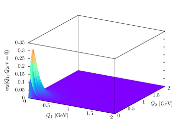
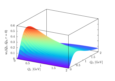
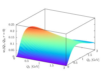
Figure 2: Model-independent weight functions for the $\pi^{0}$: $w_{1}(Q_{1},Q_{2},\tau)$ (top left) and $w_{2}(Q_{1},Q_{2},\tau)$ (top right) as function of the Euclidean momenta $Q_{1}$ and $Q_{2}$ for $\theta=90^{\circ}\leavevmode\nobreak\ (\tau=0)$. Weight functions $w_{1}(Q_{1},Q_{2},\tau)$ for $\eta$ (bottom left) and $\eta^{\prime}$ (bottom right) for $\theta=90^{\circ}$. The weight functions $w_{2}(Q_{1},Q_{2},\tau)$ for $\eta$ and $\eta^{\prime}$ have a similar shape as for the pion, but the peaks are broader.

We can immediately see from the weight functions for the pion that the low-momentum region, $Q_{1,2}\leq 0.5\leavevmode\nobreak\ \mbox{GeV}$, is the most important in the corresponding integrals (7) and (8) for $a_{\mu}^{\mathrm{HLbL};\pi^{0}}$. In $w_{1}(Q_{1},Q_{2},\tau)$ there is a peak around $Q_{1}\sim 0.15-0.19\leavevmode\nobreak\ \mbox{GeV}$, $Q_{2}\sim 0.09-0.16\leavevmode\nobreak\ \mbox{GeV}$. The values of the maxima of the weight functions for all light pseudoscalars and the locations of the maxima in the $(Q_{1},Q_{2})$-plane for a selection of $\theta$-values have been collected in Ref. Nyffeler_16 . For $w_{1}(Q_{1},Q_{2},\tau)$ and $\theta\leq 150^{\circ}$, a ridge develops along the $Q_{1}$ direction for $Q_{2}\sim 0.18-0.26\leavevmode\nobreak\ \mbox{GeV}$ (maximum along the line $Q_{1}=2\leavevmode\nobreak\ \mbox{GeV}$). For larger values of $\theta$, the function looks more and more symmetric in $Q_{1}$ and $Q_{2}$. This ridge leads for a constant form factor to an ultraviolet divergence $(\alpha/\pi)^{3}{\cal C}\ln^{2}(\Lambda/m_{\mu})$ for some momentum cutoff $\Lambda$ with ${\cal C}=3(N_{c}/(12\pi))^{2}(m_{\mu}/F_{\pi})^{2}=0.0248$, see Refs. KN_02 ; Knecht_et_al_PRL_02 . Of course, realistic form factors fall off for large momenta and $a_{\mu}^{\mathrm{HLbL};\pi^{0}(1)}$ will be convergent.

The weight function $w_{2}(Q_{1},Q_{2},\tau)$ for the pion is about an order of magnitude smaller than $w_{1}(Q_{1},Q_{2},\tau)$. There is no ridge, since the function is symmetric under $Q_{1}\leftrightarrow Q_{2}$. For $\tau$ near $-1$, the peak is around $Q_{1}=Q_{2}\sim 0.14\leavevmode\nobreak\ \mbox{GeV}$ and broader than the one shown for $\theta=90^{\circ}$. The location of the peak moves to lower values $Q_{1}=Q_{2}\sim 0.04\leavevmode\nobreak\ \mbox{GeV}$ when $\tau$ grows towards $+1$.

The dependence of the weight functions on the pseudoscalar mass through the propagators shifts the relevant momentum regions (peaks, ridges) in the weight functions, and thus also in HLbL, to higher momenta for $\eta$ compared to $\pi^{0}$ and even higher for $\eta^{\prime}$, see Fig. 2. It also leads to a suppression in the absolute size of the weight functions due to the larger masses in the propagators. This pattern is also visible in the values for the contributions to $a_{\mu}$. For the bulk of the weight functions (maxima, ridges) we observe the following approximate relations (not necessarily at the same values of the momenta and angles)

$$\left.w_{1}\right|_{\eta}\approx\frac{1}{6}\left.w_{1}\right|_{\pi^{0}},\qquad\left.w_{1}\right|_{\eta^{\prime}}\approx\frac{1}{2.5}\left.w_{1}\right|_{\eta}.$$ (9)

Of course, the ratio of the weight functions is given by the ratio of the propagators and is maximal at zero momenta and at that point equal to the ratio of the squares of the masses, but at zero momenta the weight functions themselves vanish. The combined effect is well described by the relations in Eq. (9). Furthermore, for both $\eta$ and $\eta^{\prime}$, the weight function $w_{2}$ is about a factor 20 smaller than $w_{1}$.

The peaks for the weight function $w_{1}(Q_{1},Q_{2},\tau)$ for $\eta$ and $\eta^{\prime}$ are less steep, compared to $\pi^{0}$, and the ridge is quite broad in the $Q_{2}$-direction, so that the weight function is still sizeable, compared to the maximum, for $Q_{2}=2\leavevmode\nobreak\ \mbox{GeV}$. Furthermore, the ridge falls off only slowly in the $Q_{1}$-direction. In particular for the $\eta^{\prime}$, the ridge for $\theta\leq 75^{\circ}$ is almost as big as the maximum out to values of $Q_{1}=2\leavevmode\nobreak\ \mbox{GeV}$. For $w_{2}(Q_{1},Q_{2},\tau)$ the peaks are broader and larger momenta contribute, compared to the pion.

For the $\eta$-meson, the peak in the weight function $w_{1}(Q_{1},Q_{2},\tau)$ is around $Q_{1}\sim 0.32-0.37\leavevmode\nobreak\ \mbox{GeV}$, $Q_{2}\sim 0.22-0.33\leavevmode\nobreak\ \mbox{GeV}$. The peak for the weight function $w_{2}(Q_{1},Q_{2},\tau)$ is around $Q_{1}=Q_{2}\sim 0.14\leavevmode\nobreak\ \mbox{GeV}$ for $\tau$ near $-1$ as for the pion. The location of the peak moves down to $Q_{1}=Q_{2}\sim 0.06\leavevmode\nobreak\ \mbox{GeV}$ when $\tau$ is near $+1$. For the $\eta^{\prime}$, the peak in $w_{1}(Q_{1},Q_{2},\tau)$ now occurs for even higher momenta, $Q_{1}\sim 0.41-0.51\leavevmode\nobreak\ \mbox{GeV}$, $Q_{2}\sim 0.31-0.43\leavevmode\nobreak\ \mbox{GeV}$. The locations of the peaks of $w_{2}(Q_{1},Q_{2},\tau)$ in the $(Q_{1},Q_{2})$-plane follow a similar pattern as for the $\eta$ meson.

4 Relevant momentum regions in $a_{\mu}^{\mathrm{HLbL;P}}$

In order to study the impact of different momentum regions on the pseudoscalar-pole contribution, we need, at least for the integral with the weight function $w_{1}(Q_{1},Q_{2},\tau)$ in Eq. (7), some knowledge on the form factor ${\cal F}_{{\rm P}\gamma^{*}\gamma^{*}}(-Q_{1}^{2},-Q_{2}^{2})$, since the integral diverges for a constant form factor. For illustration we take for the pion two simple models to perform the integrals: Lowest Meson Dominance with an additional vector multiplet, LMD+V model, based on the Minimal Hadronic Approximation to large-$N_{c}$ QCD matched to certain QCD short-distance constraints from the operator product expansion (OPE), see Refs. KN_EPJC_01 ; KN_02 and references therein, and the well-known Vector Meson Dominance (VMD) model. Of course, in the end, the models have to be replaced as much as possible by experimental data on the double-virtual TFF or one can use a DR for the form factor itself pion_TFF_DR .

The main difference of the models is a different behavior of the double-virtual form factor for large and equal momenta. The LMD+V model reproduces by construction the OPE, whereas the VMD TFF falls off too fast:

$${\cal F}_{\pi^{0}\gamma^{*}\gamma^{*}}^{\rm LMD+V}(-Q^{2},-Q^{2}) \!\!\!\!\!\sim\!\!\!\!\! {\cal F}_{\pi^{0}\gamma^{*}\gamma^{*}}^{\rm OPE}(-Q^{2},-Q^{2})\!\sim\!\frac{1}{Q^{2}},$$ (10)

$${\cal F}_{\pi^{0}\gamma^{*}\gamma^{*}}^{\rm VMD}(-Q^{2},-Q^{2}) \!\!\!\!\!\sim\!\!\!\!\! \frac{1}{Q^{4}},\,\quad\mbox{for large\leavevmode\nobreak\ }Q^{2}.$$ (11)

Nevertheless for not too large momenta, $Q_{1}=Q_{2}=Q=0.5\leavevmode\nobreak\ [0.75]\leavevmode\nobreak\ \mbox{GeV}$, the form factors ${\cal F}_{\pi^{0}\gamma^{*}\gamma^{*}}(-Q^{2},-Q^{2})$ in the two models differ by only $3\%\leavevmode\nobreak\ [10\%]$, see Nyffeler_16 . Furthermore, both models give an equally good description of the single-virtual TFF ${\cal F}_{\pi^{0}\gamma^{*}\gamma^{*}}(-Q^{2},0)$ KN_EPJC_01 ; KLOE2_impact .

The LMD+V model was developed in Ref. KN_EPJC_01 in the chiral limit and assuming octet symmetry. This is certainly not a good approximation for the more massive $\eta$ and $\eta^{\prime}$ mesons. For the $\eta$ and $\eta^{\prime}$ meson we therefore simply take the usual VMD model as already done in Refs. KN_02 ; N_09 .

The two models yield the following results for the pole-contribution of the light pseudoscalars to HLbL (we only list here the central values)

$$a_{\mu;{\rm LMD+V}}^{\mathrm{HLbL};\pi^{0}} = 62.9\times 10^{-11}\,,$$ (12)

$$a_{\mu;{\rm VMD}}^{\mathrm{HLbL};\pi^{0}} = 57.0\times 10^{-11}\,,$$ (13)

$$a_{\mu;{\rm VMD}}^{{\rm HLbL};\eta} = 14.5\times 10^{-11},$$ (14)

$$a_{\mu;{\rm VMD}}^{{\rm HLbL};\eta^{\prime}} = 12.5\times 10^{-11}.$$ (15)

The results (12) and (13) for the pion-pole contribution in the two models are in the ballpark of many other estimates, but they also differ by $9.4\%$, relative to the LMD+V result, due to the different high-energy behavior for the double-virtual TFF in Eqs. (10) and (11) for $Q_{1,2}\geq 1\leavevmode\nobreak\ \mbox{GeV}$. In fact, the pattern of the contributions to $a_{\mu}^{\mathrm{HLbL};\pi^{0}}$ is to a large extent determined by the model-independent weight functions $w_{1,2}(Q_{1},Q_{2},\tau)$, which are concentrated below about $0.5\leavevmode\nobreak\ \mbox{GeV}$, up to that ridge in $w_{1}$ along the $Q_{1}$ direction. As long as realistic form factor models for the double-virtual case fall off at large momenta and do not differ too much at low momenta, we expect similar results for the pion-pole contribution at the level of $15\%$ which is in fact what is seen in the literature KN_02 ; JN_09 ; HLbL_talks . Nevertheless, due to the ridge-like structure in the weight function $w_{1}$, the high-energy behavior of the form factors is relevant at the precision of $10\%$ one is aiming for.

For the $\eta$ and $\eta^{\prime}$, the results in Eqs. (14) and (15) are as expected from the discussion of the relative size of the weight functions in Eq. (9). The result for $\eta$ is about a factor 4 smaller than for the pion with VMD. The result for $\eta^{\prime}$ is only slighly smaller than for $\eta$. Note that the normalization of the TFF from $\Gamma({\rm P}\to\gamma\gamma)$ and the momentum dependence due to different vector meson masses for $\eta$ and $\eta^{\prime}$ also play a role for the results in Eqs. (14) and (15).

For a more detailed analysis, we integrate in Eqs. (7) and (8) over individual momentum bins and all angles $\theta$

$$\int_{Q_{1,{\rm min}}}^{Q_{1,{\rm max}}}dQ_{1}\int_{Q_{2,{\rm min}}}^{Q_{2,{\rm max}}}dQ_{2}\int_{-1}^{1}d\tau$$ (16)

and display the results, relative to the totals in Eqs. (12)-(15), in Fig. 3.

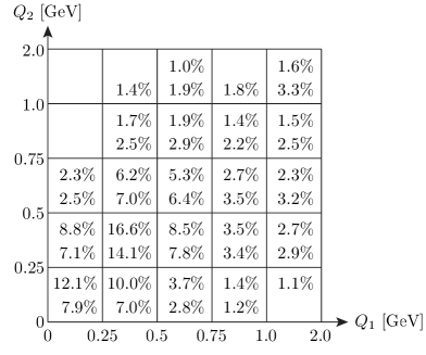
Figure 3: Left panel: Relative contributions to the total $a_{\mu}^{\mathrm{HLbL};\pi^{0}}$ from individual bins in the $(Q_{1},Q_{2})$-plane, integrated over all angles according to Eq. (16). Note the larger size of the bins with $Q_{1,2}\geq 1\leavevmode\nobreak\ \mbox{GeV}$. Top line in each bin: LMD+V model, bottom line: VMD model. Contributions smaller than 1% have not been displayed. For the LMD+V model there are further contributions bigger than 1% along the $Q_{1}$-axis. For $2\leavevmode\nobreak\ \mbox{GeV}\leq Q_{1}\leq 20\leavevmode\nobreak\ \mbox{GeV}$: $1.1\%$ in the bin $0\leq Q_{2}\leq 0.25\leavevmode\nobreak\ \mbox{GeV}$ and $1.2\%$ for $0.25\leavevmode\nobreak\ \mbox{GeV}\leq Q_{2}\leq 0.5\leavevmode\nobreak\ \mbox{GeV}$. Right panel: Relative contributions to the total of $a_{\mu}^{{\rm HLbL};\eta}$ and $a_{\mu}^{{\rm HLbL};\eta^{\prime}}$ with the VMD model from individual bins in the $(Q_{1},Q_{2})$-plane, integrated over all angles. Top line in each bin: $\eta$-meson, bottom line: $\eta^{\prime}$-meson.

Since the absolute size of the weight function $w_{1}(Q_{1},Q_{2},\tau)$ is much larger than $w_{2}(Q_{1},Q_{2},\tau)$, the contribution from the integral $a_{\mu}^{\mathrm{HLbL};\pi^{0}(1)}$ in Eq. (7) dominates over $a_{\mu}^{\mathrm{HLbL};\pi^{0}(2)}$ in Eq. (8). Therefore the asymmetry seen in the $(Q_{1},Q_{2})$-plane in Fig. 3, with larger contributions below the diagonal, reflects the ridge-like structure of $w_{1}(Q_{1},Q_{2},\tau)$ in Fig. 2.

For the pion, the largest contribution comes from the lowest bin $Q_{1,2}\leq 0.25\leavevmode\nobreak\ \mbox{GeV}$ since a large part of the peaks in the weight functions (for different angles $\theta$) is contained in that bin. More than half of the contribution comes from the four bins with $Q_{1,2}\leq 0.5\leavevmode\nobreak\ \mbox{GeV}$. In contrast, for the $\eta$ and $\eta^{\prime}$, it is not the bin $Q_{1,2}\leq 0.25\leavevmode\nobreak\ \mbox{GeV}$ which yields the largest contribution, since the maxima of the weight functions are shifted to higher momenta, around $0.3-0.5\leavevmode\nobreak\ \mbox{GeV}$. Furthermore, more bins up to $Q_{2}=2\leavevmode\nobreak\ \mbox{GeV}$ now contribute at least $1\%$ to the total. This is different from the pattern seen for $\pi^{0}$. The plots of the weight functions for $\eta$ and $\eta^{\prime}$ in Fig. 2 show that now the region $1.5-2.5\leavevmode\nobreak\ \mbox{GeV}$ also is important for the evaluation of the $\eta$- and $\eta^{\prime}$-pole contributions. The VMD model is, however, known to have a too fast fall-off at large momenta, compared to the OPE. Therefore the size of the contributions $a_{\mu}^{{\rm HLbL};\eta}$ and $a_{\mu}^{{\rm HLbL};\eta^{\prime}}$ in Eqs. (14) and (15) might be underestimated by the VMD model, which could also affect the relative importance of the higher momentum region in Fig. 3.

Integrating both $Q_{1}$ and $Q_{2}$ from zero up to some upper momentum cutoff $\Lambda$ and integrating over all angles $\theta$, one obtains the results shown in Table 1. This amounts to summing up the individual bins shown in Fig. 3.

Table 1: Pseudoscalar-pole contribution $a_{\mu}^{\mathrm{HLbL;P}}\times 10^{11},{\rm P}=\pi^{0},\eta,\eta^{\prime}$ for different form factor models obtained with a momentum cutoff $\Lambda$. In brackets, relative contribution of the total obtained with $\Lambda=20\leavevmode\nobreak\ \mbox{GeV}$.

$\Lambda$ [GeV]		$\pi^{0}$ [LMD+V]		$\pi^{0}$ [VMD]		$\eta$ [VMD]		$\eta^{\prime}$ [VMD]
0.	25	14.	4 (22.9%)	14.	4 (25.2%)	1.	8 (12.1%)	1.	0 (7.9%)
0.	5	36.	8 (58.5%)	36.	6 (64.2%)	6.	9 (47.5%)	4.	5 (36.1%)
0.	75	48.	5 (77.1%)	47.	7 (83.8%)	10.	7 (73.4%)	7.	8 (62.5%)
1.	0	54.	1 (86.0%)	52.	6 (92.3%)	12.	6 (86.6%)	9.	9 (79.1%)
1.	5	58.	8 (93.4%)	55.	8 (97.8%)	14.	0 (96.1%)	11.	7 (93.1%)
2.	0	60.	5 (96.2%)	56.	5 (99.2%)	14.	3 (98.6%)	12.	2 (97.4%)
5.	0	62.	5 (99.4%)	56.	9 (99.9%)	14.	5 (100%)	12.	5 (99.9%)
20.	0	62.	9 (100%)	57.	0 (100%)	14.	5 (100%)	12.	5 (100%)

As one can see in Table 1, for the pion more than half of the final result stems from the region below $\Lambda=0.5\leavevmode\nobreak\ \mbox{GeV}$ (59% for LMD+V, 64% for VMD) and the region below $\Lambda=1\leavevmode\nobreak\ \mbox{GeV}$ gives the bulk of the total result (86% for LMD+V, 92% for VMD). The small difference between the form factor models for small momenta $Q_{1,2}\leq 0.5\leavevmode\nobreak\ \mbox{GeV}$ is reflected in the small absolute difference for $a_{\mu}^{\mathrm{HLbL};\pi^{0}}$ in the two models for $\Lambda\leq 0.75\leavevmode\nobreak\ \mbox{GeV}$. For instance, for $\Lambda=0.75\leavevmode\nobreak\ \mbox{GeV}$, the difference is only $0.8\times 10^{-11}$, i.e. $1.6\%$. The faster fall-off of the VMD model at larger momenta beyond $1\leavevmode\nobreak\ \mbox{GeV}$, compared to the LMD+V model, leads to a smaller contribution from that region to the total. Therefore we can see in Fig. 3 that the main contributions in the VMD model, relative to the total, are concentrated at lower momenta, compared to the LMD+V model, in particular below $0.75\leavevmode\nobreak\ \mbox{GeV}$.

On the other hand, Table 1 shows that for $\eta$ and $\eta^{\prime}$, the region below $\Lambda=0.25\leavevmode\nobreak\ \mbox{GeV}$ only gives a small contribution to the total (12% for $\eta$, 8% for $\eta^{\prime}$). Up to $\Lambda=0.5\leavevmode\nobreak\ \mbox{GeV}$, we get about half (one third) for $\eta$ ($\eta^{\prime}$) and the bulk of the results comes from the region below $\Lambda=1.5\leavevmode\nobreak\ \mbox{GeV}$, 96% for the $\eta$ and 93% for the $\eta^{\prime}$-meson.

5 Impact of transition form factor uncertainties on $a_{\mu}^{\mathrm{HLbL;P}}$

For the calculation of the pseudoscalar-pole contribution $a_{\mu}^{\mathrm{HLbL;P}}$ with ${\rm P}=\pi^{0},\eta,\eta^{\prime}$ in Eqs. (7) and (8) the single-virtual form factor ${\cal F}_{{\rm P}\gamma^{*}\gamma^{*}}(-Q^{2},0)$ and the double-virtual form factor ${\cal F}_{{\rm P}\gamma^{*}\gamma^{*}}(-Q_{1}^{2},-Q_{2}^{2})$, both in the spacelike region, enter. We are interested here in the impact of uncertainties of experimental measurements of these form factors on the precision of $a_{\mu}^{\mathrm{HLbL;P}}$. See Ref. TFF for a brief overview of the various experimental processes where information on the transition form factors can be obtained. In the following, we will only quote the most relevant and most precise experimental references. Ref. Nyffeler_16 contains a detailed analysis of the current experimental situation.

For the single-virtual form factor ${\cal F}_{{\rm P}\gamma^{*}\gamma^{*}}(-Q^{2},0)$ the following experimental information is available. The normalization of the form factor can be obtained from the decay width $\Gamma({\rm P}\to\gamma\gamma)$ PDG_2014 ; P_to_gamma_gamma . Another important experimental information is the slope of the form factor at the origin. In the spacelike region, the slope and the form factor itself have been measured in the process $e^{+}e^{-}\to e^{+}e^{-}\gamma^{*}\gamma^{*}\to e^{+}e^{-}{\rm P}$ TFF_spacelike . The extraction of the slope requires, however, a model dependent extrapolation from rather large momenta $Q\sim 0.5\leavevmode\nobreak\ \mbox{GeV}$ to $Q^{2}=0$. The slope and the TFF can also be obtained in the timelike region from the single Dalitz-decay ${\rm P}\to\gamma^{*}\gamma\to\ell^{+}\ell^{-}\gamma$ with $\ell=e,\mu$ TFF_timelike . Of course, for the pion only the decay with an electron pair is possible. For the pion the phase space is, however, rather small and the decay is not very sensitive to form factor effects. The corresponding determinations of the slope and the TFF are rather unprecise. The situation is much better for $\eta$ and $\eta^{\prime}$. However, one then still needs to perform an analytical continuation to obtain the form factor at spacelike momenta. Recently a DR has been proposed in Ref. pion_TFF_DR to determine the single- and double-virtual form factor for the pion. So far, only the single-virtual form factor has been evaluated in this dispersive framework with high precision at low momenta $Q\leq 1\leavevmode\nobreak\ \mbox{GeV}$. For the $\eta$ and $\eta^{\prime}$, a dispersive approach for the single- and double-virtual TFF has been presented in Ref. eta_etaprime_TFF_DR .

For the single-virtual form factor we parametrize the measurement errors in Eqs. (7) and (8) as follows:

$${\cal F}_{{\rm P}\gamma^{*}\gamma^{*}}(-Q^{2},0)\to{\cal F}_{{\rm P}\gamma^{*}\gamma^{*}}(-Q^{2},0)\,\left(1\pm\delta_{1,{\rm P}}(Q)\right).$$ (17)

The momentum dependent errors $\delta_{1,{\rm P}}(Q)$ in different bins are displayed in Table 2, based on the analysis in Ref. Nyffeler_16 . There are currently no experimental data for the form factor available in the spacelike region in the lowest bin $0\leq Q<0.5\leavevmode\nobreak\ \mbox{GeV}$ for $\pi^{0}$ and $\eta$, except from $\Gamma({\rm P}\to\gamma\gamma)$, the slope and timelike data for the $\eta$-TFF. For the lowest bin we therefore assume an error, based on “extrapolating” the current data sets and the data that will be available soon from BESIII BESIII_private and maybe from KLOE-2 KLOE2_impact for the pion. If one uses the DR from Ref. pion_TFF_DR below $1\leavevmode\nobreak\ \mbox{GeV}$ pion_TFF_DR_private and the current error on the normalization from the decay width, one obtains (conservatively) the uncertainties in the lowest two bins given in brackets in Table 2.

Table 2: Relative error $\delta_{1,{\rm P}}(Q)$ on the form factor ${\cal F}_{{\rm P}\gamma^{*}\gamma^{*}}(-Q^{2},0)$ for ${\rm P}=\pi^{0},\eta,\eta^{\prime}$ in different momentum regions. The errors for $\delta_{1,\pi^{0}}(Q)$ and $\delta_{1,\eta}(Q)$ below $0.5\leavevmode\nobreak\ \mbox{GeV}$ are based on assumptions. In brackets for $\pi^{0}$ the uncertainties with a DR for the TFF.

Region [GeV]		$\delta_{1,\pi^{0}}(Q)$		$\delta_{1,\eta}(Q)$		$\delta_{1,\eta^{\prime}}(Q)$
$0\leq$$\leavevmode\nobreak\ Q\leavevmode\nobreak\$	$<0.5$	5%	[2%]	10%		6%
$0.5\leq$$\leavevmode\nobreak\ Q\leavevmode\nobreak\$	$<1$	7%	[4%]	15%		11%
$1\leq$$\leavevmode\nobreak\ Q\leavevmode\nobreak\$	$<2$	8%		8%		7%
$2\leq$$\leavevmode\nobreak\ Q\leavevmode\nobreak\$		4%		4%		4%

The second ingredient in Eqs. (7) and (8) is the double-virtual form factor ${\cal F}_{{\rm P}\gamma^{*}\gamma^{*}}(-Q_{1}^{2},-Q_{2}^{2})$. Currently, there are no direct experimental measurements available for this form factor at spacelike momenta. For the pion, from the double Dalitz decay $\pi^{0}\to\gamma^{*}\gamma^{*}\to e^{+}e^{-}e^{+}e^{-}$, one can obtain the double-virtual form factor $|{\cal F}_{\pi^{0}\gamma^{*}\gamma^{*}}(q_{1}^{2},q_{2}^{2})|$ at small invariant momenta in the timelike region, but the results are inconclusive double_Dalitz . There is indirect information available on the double-virtual TFF from the loop-induced decay ${\rm P}\to\ell^{+}\ell^{-}\leavevmode\nobreak\ (\ell=e,\mu)$ PDG_2014 ; P_to_ll . Without a form factor at the ${\rm P}-\gamma^{*}-\gamma^{*}$-vertex, the loop integral is ultraviolet divergent. The relation between this decay and the pseudoscalar-pole contribution $a_{\mu}^{\mathrm{HLbL;P}}$ has been stressed in Ref. Knecht_et_al_PRL_02 and problems to explain both processes simultaneously with the same model have been pointed out HLbL_PS_vs_lepton_pair_decay .

In this situation, models have been used to describe the form factor ${\cal F}_{{\rm P}\gamma^{*}\gamma^{*}}(-Q_{1}^{2},-Q_{2}^{2})$ in the spacelike region and thus all current evaluations of $a_{\mu}^{\mathrm{HLbL;P}}$ are model dependent. Of course, it would be preferable to replace these model assumptions as much as possible by experimental data. In fact, it is planned to determine the double-virtual form factor, at least for the pion, at BESIII for momenta $0.5\leq Q_{1,2}\leq 1.5\leavevmode\nobreak\ \mbox{GeV}$ and a first analysis is already in progress BESIII_private , based on existing data.

In analogy to the single-virtual form factor, we parametrize potential future measurement errors for the double-virtual form factor in Eqs. (7) and (8) in the following, simplifying way:

$${\cal F}_{{\rm P}\gamma^{*}\gamma^{*}}(-Q_{1}^{2},-Q_{2}^{2})$$ (18)

$$\to{\cal F}_{{\rm P}\gamma^{*}\gamma^{*}}(-Q_{1}^{2},-Q_{2}^{2})\,\left(1\pm\delta_{2,{\rm P}}(Q_{1},Q_{2})\right),$$

where the assumed momentum dependent errors $\delta_{2,{\rm P}}(Q_{1},Q_{2})$ in different bins are shown in Fig. 4. The error estimate for the form factor in each bin has been obtained based on a Monte Carlo (MC) simulation BESIII_private for the BESIII detector using the LMD+V model in the EKHARA event generator EKHARA for the signal process $e^{+}e^{-}\to e^{+}e^{-}\gamma^{*}\gamma^{*}\to e^{+}e^{-}\pi^{0}$ and the VMD model for the production of $\eta$ and $\eta^{\prime}$. Since the number of events $N_{i}$ in bin number $i$ is proportional to the cross-section $\sigma_{i}$ (in that bin) and since for the calculation of the cross-section the form factor enters squared, the statistical error on the form factor measurement is given according to Poisson statistics by $\sigma_{i}\sim{\cal F}_{{\rm P}\gamma^{*}\gamma^{*}}^{2}\Rightarrow\delta{\cal F}_{{\rm P}\gamma^{*}\gamma^{*}}/{\cal F}_{{\rm P}\gamma^{*}\gamma^{*}}=\sqrt{N_{i}}/(2N_{i})$.

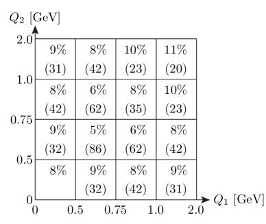
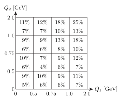
Figure 4: Left panel: Assumed relative error $\delta_{2,\pi^{0}}(Q_{1},Q_{2})$ on the pion TFF ${\cal F}_{\pi^{0}\gamma^{*}\gamma^{*}}(-Q_{1}^{2},-Q_{2}^{2})$ in different momentum bins. Note the unequal bin sizes. In brackets the number of MC events $N_{i}$ in each bin according to the simulation with the LMD+V model for BESIII. For the lowest bin, $Q_{1,2}\leq 0.5\leavevmode\nobreak\ \mbox{GeV}$, there are no events in the simulation due to the detector acceptance. In that bin, we assume as error the average of the three neighboring bins. For $Q_{1,2}\geq 2\leavevmode\nobreak\ \mbox{GeV}$, we take a constant error of 15%. Right panel: Assumed relative error $\delta_{2,{\rm P}}(Q_{1},Q_{2})$ on the form factor ${\cal F}_{{\rm P}\gamma^{*}\gamma^{*}}(-Q_{1}^{2},-Q_{2}^{2})$ for $P=\eta,\eta^{\prime}$ in different momentum bins according to the MC simulations with the VMD form factor for $\eta$ (top line) and $\eta^{\prime}$ (bottom line). For $Q_{1,2}\geq 2\leavevmode\nobreak\ \mbox{GeV}$, we assume a constant error of 25% for $\eta$ and 15% for $\eta^{\prime}$.

In the lowest momentum bin $Q_{1,2}\leq 0.5\leavevmode\nobreak\ \mbox{GeV}$, there are no events in the simulation, because of the acceptance of the detector. When both $Q_{1,2}^{2}$ are small, both photons are almost real and the scattered electrons and positrons escape detection along the beam pipe. As a further assumption, we have therefore taken the average of the uncertainties in the three neighboring bins as estimate for the error in that lowest bin. This “extrapolation” from the neighboring bins seems justified, since information along the two axis is (or will soon be) available and the value at the origin is known quite precisely from the decay width. Note that although the form factor for spacelike momenta is rather smooth, it is far from being a constant and some nontrivial extrapolation is needed. For instance, for the pion we get ${\cal F}_{\pi^{0}\gamma^{*}\gamma^{*}}(-(0.5\leavevmode\nobreak\ \mbox{GeV})^{2},-(0.5\leavevmode\nobreak\ \mbox{GeV})^{2})/{\cal F}_{\pi^{0}\gamma^{*}\gamma^{*}}(0,0)\approx 0.5$, for both the LMD+V and the VMD model Nyffeler_16 .

The MC simulation BESIII_private corresponds to a data sample of approximately half of the data collected at BESIII so far. The simulation included only signal events. Based on a first preliminary analysis of the BESIII data BESIII_private with strong cuts to reduce the background from Bhabha events with additional photons, it seems possible, at least for the pion, that the number of events and the corresponding precision for ${\cal F}_{\pi^{0}\gamma^{*}\gamma^{*}}(-Q_{1}^{2},-Q_{2}^{2})$ shown in Fig. 4 could be achievable with the current data set plus a few more years of data taking. Of course, once experimental data will be available, e.g. event rates in the different momentum bins, there will still be the task to unfold the data to reconstruct the form factor ${\cal F}_{{\rm P}\gamma^{*}\gamma^{*}}(-Q_{1}^{2},-Q_{2}^{2})$ without introducing too much model dependence.

Taking the LMD+V and VMD models for illustration, the assumed momentum dependent errors from Table 2 and Fig. 4 impact the precision for the pseudoscalar-pole contributions to HLbL as follows

$$a_{\mu;{\rm LMD+V}}^{\mathrm{HLbL};\pi^{0}} = {62.9}^{+8.9}_{-8.2}\times 10^{-11}\quad\left({}^{+14.1\%}_{-13.1\%}\right),$$ (19)

$$a_{\mu;{\rm VMD}}^{\mathrm{HLbL};\pi^{0}} = {57.0}^{+7.8}_{-7.3}\times 10^{-11}\quad\left({}^{+13.7\%}_{-12.7\%}\right),$$ (20)

$$a_{\mu;{\rm VMD}}^{{\rm HLbL};\eta} = 14.5^{+3.4}_{-3.0}\times 10^{-11}\quad\left({}^{+23.4\%}_{-20.8\%}\right),$$ (21)

$$a_{\mu;{\rm VMD}}^{{\rm HLbL};\eta^{\prime}} = 12.5^{+1.9}_{-1.7}\times 10^{-11}\quad\left({}^{+15.1\%}_{-13.9\%}\right).$$ (22)

While for the pion the absolute variations are different for the two models, as are the central values, the relative uncertainty for both models is around $14\%$. This will also be visible in the following more detailed analysis. We therefore expect that using other form factor models, and, eventually, using experimental data for the single- and double-virtual form factors, will not substantially change the following observations and conclusions.

More details have been collected in Table 3, which contains the results for the relative uncertainties from Eqs. (19)-(22) in the first line. For the pion, the largest uncertainty of about $5\%$ comes from the lowest bin $Q_{1,2}\leq 0.5\leavevmode\nobreak\ \mbox{GeV}$ in the $(Q_{1},Q_{2})$-plane for $\delta_{2}$ in Fig. 4 (fourth line in the table). Some improvement could be achieved, if the error in that lowest bin and the neighboring bins could be reduced, to a total error of about $12\%$, see the lines 8 and 9 in Table 3. The second largest uncertainty of $4.4\%$ for the pion stems from the lowest bin $Q<0.5\leavevmode\nobreak\ \mbox{GeV}$ in $\delta_{1}$ (second line in the table). Here the use of a dispersion relation for the single-virtual form factor ${\cal F}_{\pi^{0}\gamma^{*}\gamma^{*}}(-Q^{2},0)$ for $Q<1\leavevmode\nobreak\ \mbox{GeV}$ (see values in brackets in Table 2) could bring the total error of $14\%$ down to $11\%$, see the sixth line.

For the $\eta$ meson, the largest uncertainties of $7\%$ originate from the region of $\delta_{2}$ above $0.5\leavevmode\nobreak\ \mbox{GeV}$ (5th line) and from the lowest bin in $\delta_{1}$ (2nd line). For the $\eta^{\prime}$, the largest uncertainty of $5\%$ comes again from the region of $\delta_{2}$ above $0.5\leavevmode\nobreak\ \mbox{GeV}$ (5th line). The second largest uncertainty of $4.5\%$ comes from bins in $\delta_{1}$ above $0.5\leavevmode\nobreak\ \mbox{GeV}$ (3rd line). For $\eta$ and $\eta^{\prime}$ the errors go down to $20\%$ and $13\%$, if the uncertainty in the two lowest bins in $\delta_{1}$ could be reduced, see line 7 in Table 3. There is only a small reduction of the uncertainty by one percentage point, if the errors in the lowest few bins of $\delta_{2}$ could be reduced further, see lines 8 and 9.

Table 3: Impact of assumed measurement errors $\delta_{1,{\rm P}}(Q)$ and $\delta_{2,{\rm P}}(Q_{1},Q_{2})$ in the form factors ${\cal F}_{{\rm P}\gamma^{*}\gamma^{*}}(-Q^{2},0)$ and ${\cal F}_{{\rm P}\gamma^{*}\gamma^{*}}(-Q_{1}^{2},-Q_{2}^{2})$ on the relative precision of the pseudoscalar-pole contributions (first line). Lines $2-5$ show the effects of uncertainties in different momentum regions below and above $0.5\leavevmode\nobreak\ \mbox{GeV}$. Lines $6-9$ show the impact of potential improvements of some of the assumed errors.

$\frac{\delta a_{\mu;{\rm LMD+V}}^{\mathrm{HLbL};\pi^{0}}}{a_{\mu;{\rm LMD+V}}^{\mathrm{HLbL};\pi^{0}}}$	$\frac{\delta a_{\mu;{\rm VMD}}^{\mathrm{HLbL};\pi^{0}}}{a_{\mu;{\rm VMD}}^{\mathrm{HLbL};\pi^{0}}}$	$\frac{\delta a_{\mu;{\rm VMD}}^{{\rm HLbL};\eta}}{a_{\mu;{\rm VMD}}^{{\rm HLbL};\eta}}$	$\frac{\delta a_{\mu;{\rm VMD}}^{{\rm HLbL};\eta^{\prime}}}{a_{\mu;{\rm VMD}}^{{\rm HLbL};\eta^{\prime}}}$	Comment
${}^{+14.1\%}_{-13.1\%}$	${}^{+13.7\%}_{-12.7\%}$	${}^{+23.4\%}_{-20.8\%}$	${}^{+15.1\%}_{-13.9\%}$	Given $\delta_{1},\delta_{2}$
${}^{+4.3\%}_{-4.2\%}$	${}^{+4.4\%}_{-4.3\%}$	${}^{+6.9\%}_{-6.8\%}$	${}^{+3.4\%}_{-3.3\%}$	Bin $Q<0.5\leavevmode\nobreak\ \mbox{GeV}$ in $\delta_{1}$ as given, rest: $\delta_{1,2}=0$
${}^{+1.1\%}_{-1.0\%}$	${}^{+1.0\%}_{-0.9\%}$	${}^{+4.4\%}_{-4.3\%}$	${}^{+4.5\%}_{-4.4\%}$	Bins $Q\geq 0.5\leavevmode\nobreak\ \mbox{GeV}$ in $\delta_{1}$ as given, rest: $\delta_{1,2}=0$
${}^{+4.5\%}_{-4.4\%}$	${}^{+4.9\%}_{-4.8\%}$	${}^{+4.0\%}_{-4.0\%}$	${}^{+1.7\%}_{-1.7\%}$	Bin $Q_{1,2}<0.5\leavevmode\nobreak\ \mbox{GeV}$ in $\delta_{2}$ as given, rest: $\delta_{1,2}=0$
${}^{+3.9\%}_{-3.8\%}$	${}^{+3.2\%}_{-3.1\%}$	${}^{+7.0\%}_{-6.8\%}$	${}^{+5.1\%}_{-5.0\%}$	Bins $Q_{1,2}\geq 0.5\leavevmode\nobreak\ \mbox{GeV}$ in $\delta_{2}$ as given, rest: $\delta_{1,2}=0$
${}^{+10.9\%}_{-10.5\%}$	${}^{+10.6\%}_{-10.1\%}$	$-$	$-$	$\pi^{0}$: given $\delta_{1},\delta_{2}$, but two lowest bins in $\delta_{1,\pi^{0}}$ from DR: $2\%,4\%$
$-$	$-$	${}^{+20.4\%}_{-18.5\%}$	${}^{+13.4\%}_{-12.5\%}$	$\eta,\eta^{\prime}$: given $\delta_{1},\delta_{2}$, but two lowest bins in $\delta_{1,\eta}$: $8\%,10\%$ and $\delta_{1,\eta^{\prime}}$: $5\%,8\%$
${}^{+12.4\%}_{-11.6\%}$	${}^{+11.8\%}_{-11.0\%}$	${}^{+22.4\%}_{-20.0\%}$	${}^{+14.8\%}_{-13.6\%}$	For $\pi^{0},\eta,\eta^{\prime}$: given $\delta_{1},\delta_{2}$, but lowest bin in $\delta_{2}$: $8\%,9\%,5\%\to 5\%,7\%,4\%$
${}^{+12.0\%}_{-11.2\%}$	${}^{+11.4\%}_{-10.6\%}$	${}^{+21.9\%}_{-19.6\%}$	${}^{+14.4\%}_{-13.4\%}$	In addition, bins in $\delta_{2}$ close to lowest bin: $9\%,10\%,6\%\to 5\%,7\%,4\%$

6 Conclusions

The three-dimensional integral representation for the pseudoscalar-pole contribution $a_{\mu}^{\mathrm{HLbL;P}}$ with ${\rm P}=\pi^{0},\eta,\eta^{\prime}$, from Ref. JN_09 allows one to separate the generic kinematics, described by model-independent weight functions $w_{1,2}(Q_{1},Q_{2},\tau)$, from the double-virtual transition form factors ${\cal F}_{{\rm P}\gamma^{*}\gamma^{*}}(-Q_{1}^{2},-Q_{2}^{2})$. From the weight functions one deduces that the relevant momentum regions are below $1\leavevmode\nobreak\ \mbox{GeV}$ for $\pi^{0}$ and below about $1.5\leavevmode\nobreak\ \mbox{GeV}$ for $\eta$ and $\eta^{\prime}$.

If the assumed measurement errors $\delta_{1,{\rm P}}(Q)$ and $\delta_{2,{\rm P}}(Q_{1},Q_{2})$ on the single- and double-virtual TFF can be achieved in the coming years (in particular by measurements of the double-virtual form factors at BESIII), one could obtain the following, largely data driven, uncertainties for the pseudoscalar-pole contributions to HLbL:

$$\delta a_{\mu}^{\mathrm{HLbL};\pi^{0}}/a_{\mu}^{\mathrm{HLbL};\pi^{0}} = 14\%\quad[11\%],$$ (23)

$$\delta a_{\mu}^{{\rm HLbL};\eta}/a_{\mu}^{{\rm HLbL};\eta} = 23\%,$$ (24)

$$\delta a_{\mu}^{{\rm HLbL};\eta^{\prime}}/a_{\mu}^{{\rm HLbL};\eta^{\prime}} = 15\%.$$ (25)

The result in bracket for the pion uses the DR pion_TFF_DR for the single-virtual TFF ${\cal F}_{\pi^{0}\gamma^{*}\gamma^{*}}(-Q^{2},0)$. Compared to the range of estimates in the literature given in Eqs. (3) and (4) this would definitely be some progress. More work is needed, however, to reach a precision of $10\%$ for all three contributions. Experimental data on the double-virtual form factors in the region $0-1.5\leavevmode\nobreak\ \mbox{GeV}$, e.g. from KLOE-2 or Belle 2, would be very helpful in this respect. A more detailed discussion can be found in Nyffeler_16 .

I would like to thank the organizers for creating such a stimulating and nice atmosphere. I am grateful to Achim Denig, Christoph Redmer and Pascal Wasser for providing me with preliminary results of MC simulations for transition form factor measurements at BESIII and to Martin Hoferichter and Bastian Kubis for sharing information about the precision of the DR approach to the pion TFF. I thank the Heinrich Greinacher Foundation, University of Bern, Switzerland, for financial support. This work was supported by Deutsche Forschungsgemeinschaft (DFG) through the Collaborative Research Center “The Low-Energy Frontier of the Standard Model” (SFB 1044).

References

- (1) F. Jegerlehner and A. Nyffeler, Phys. Rept. 477, 1 (2009).
- (2) G. W. Bennett et al. [Muon g-2 Collaboration], Phys. Rev. D 73, 072003 (2006).
- (3) T. Blum et al., arXiv:1311.2198; talks at this meeting: M. Knecht; K. Melnikov.
- (4) D. Hertzog, talk at this meeting, arXiv:1512.00928 [hep-ex].
- (5) Talks on HVP at this meeting: M. Benayoun, arXiv:1511.01329 [hep-ph]; S. Eidelman; F. Jegerlehner, arXiv:1511.04473 [hep-ph]; M. Petschlies (F. Burger et al., arXiv:1511.04959 [hep-lat]); M. Steinhauser (A. Kurz et al., arXiv:1511.08222 [hep-ph]); L. Trentadue; Z. Zhang, arXiv:1511.05405 [hep-ph].
- (6) J. Prades, E. de Rafael and A. Vainshtein, Adv. Ser. Direct. High Energy Phys. 20, 303 (2009) [arXiv:0901.0306 [hep-ph]].
- (7) A. Nyffeler, Phys. Rev. D 79, 073012 (2009).
- (8) M. Hayakawa, T. Kinoshita and A. I. Sanda, Phys. Rev. Lett. 75, 790 (1995); Phys. Rev. D 54, 3137 (1996); M. Hayakawa and T. Kinoshita, Phys. Rev. D 57, 465 (1998) [66, 019902(E) (2002)].
- (9) J. Bijnens, E. Pallante and J. Prades, Phys. Rev. Lett. 75, 1447 (1995) [75, 3781(E) (1995)]; Nucl. Phys. B 474, 379 (1996); Nucl. Phys. B 626, 410 (2002).
- (10) M. Knecht and A. Nyffeler, Phys. Rev. D 65, 073034 (2002).
- (11) M. Knecht et al., Phys. Rev. Lett. 88, 071802 (2002).
- (12) K. Melnikov and A. Vainshtein, Phys. Rev. D 70, 113006 (2004).
- (13) T. Blum et al., Phys. Rev. Lett. 114, 012001 (2015); T. Blum et al., Phys. Rev. D 93, 014503 (2016).
- (14) J. Green et al., Phys. Rev. Lett. 115, 222003 (2015); J. Green et al., arXiv:1510.08384 [hep-lat].
- (15) Talks on HLbL at this meeting: J. Bijnens, arXiv:1510.05796; L. Cappiello; D. Greynat; C. Lehner; P. Masjuan; M. Procura.
- (16) G. Colangelo et al., JHEP 1409, 091 (2014); G. Colangelo et al., Phys. Lett. B 738, 6 (2014); G. Colangelo et al., JHEP 1509, 074 (2015).
- (17) V. Pauk and M. Vanderhaeghen, arXiv:1403.7503 [hep-ph]; Phys. Rev. D 90, 113012 (2014).
- (18) A. Vainshtein, talk at this meeting.
- (19) E. Czerwinski et al., arXiv:1207.6556 [hep-ph]; talks at this meeting: A. Kupsc; P. Masjuan (P. Masjuan and P. Sanchez-Puertas, arXiv:1512.09018 [hep-ph]).
- (20) A. Nyffeler, arXiv:1602.03398 [hep-ph].
- (21) M. Hoferichter et al., Eur. Phys. J. C 74, 3180 (2014).
- (22) C. Hanhart et al., Eur. Phys. J. C 73, 2668 (2013) [75, 242(E) (2015)]; C. W. Xiao et al., arXiv:1509.02194 [hep-ph].
- (23) M. Knecht and A. Nyffeler, Eur. Phys. J. C 21, 659 (2001).
- (24) D. Babusci et al., Eur. Phys. J. C 72, 1917 (2012); D. Moricciani, talk at this meeting.
- (25) K. A. Olive et al. [Particle Data Group], Chin. Phys. C 38, 090001 (2014).
- (26) I. Larin et al. [PrimEx Collaboration], Phys. Rev. Lett. 106, 162303 (2011); D. Babusci et al. [KLOE-2 Collaboration], JHEP 1301, 119 (2013).
- (27) H. Aihara et al. [TPC/Two Gamma Collaboration], Phys. Rev. Lett. 64, 172 (1990); H. J. Behrend et al. [CELLO Collaboration], Z. Phys. C 49, 401 (1991); J. Gronberg et al. [CLEO Collaboration], Phys. Rev. D 57, 33 (1998); M. Acciarri et al. [L3 Collaboration], Phys. Lett. B 418, 399 (1998); B. Aubert et al. [BaBar Collaboration], Phys. Rev. D 80, 052002 (2009); P. del Amo Sanchez et al. [BaBar Collaboration], Phys. Rev. D 84, 052001 (2011); S. Uehara et al. [Belle Collaboration], Phys. Rev. D 86, 092007 (2012).
- (28) R. Arnaldi et al. [NA60 Collaboration], Phys. Lett. B 677, 260 (2009); P. Aguar-Bartolome et al. [A2 Collaboration], Phys. Rev. C 89, 044608 (2014); M. Ablikim et al. [BESIII Collaboration], Phys. Rev. D 92, 012001 (2015).
- (29) A. Denig, C. Redmer and P. Wasser, private communication.
- (30) M. Hoferichter and B. Kubis, private communication.
- (31) E. Abouzaid et al. [KTeV Collaboration], Phys. Rev. Lett. 100, 182001 (2008).
- (32) E. Abouzaid et al. [KTeV Collaboration], Phys. Rev. D 75, 012004 (2007).
- (33) M. J. Ramsey-Musolf and M. B. Wise, Phys. Rev. Lett. 89, 041601 (2002); A. E. Dorokhov and M. A. Ivanov, JETP Lett. 87, 531 (2008); P. Masjuan and P. Sanchez-Puertas, arXiv:1504.07001 [hep-ph].
- (34) H. Czyż and S. Ivashyn, Comput. Phys. Commun. 182, 1338 (2011); H. Czyż et al., Phys. Rev. D 85, 094010 (2012).