Momentum structure of the self-energy and its parametrization for the two-dimensional Hubbard model

Abstract

We compute the self-energy for the half-filled Hubbard model on a square lattice using lattice quantum Monte Carlo simulations and the dynamical vertex approximation. The self-energy is strongly momentum-dependent, but it can be parametrized via the non-interacting energy-momentum dispersion $\varepsilon_{\mathbf{k}}$, except for pseudogap features right at the Fermi edge. That is, it can be written as $\Sigma(\varepsilon_{\mathbf{k}},\omega)$, with two energy-like parameters ($\varepsilon$, $\omega$) instead of three ($k_{x}$, $k_{y}$ and $\omega$). The self-energy has two rather broad and weakly dispersing high energy features and a sharp $\omega=\varepsilon_{\mathbf{k}}$ feature at high temperatures, which turns to $\omega=-\varepsilon_{\mathbf{k}}$ at low temperatures. Altogether this yields a Z- and Z -like structure, respectively, for the imaginary part of $\Sigma(\varepsilon_{\mathbf{k}},\omega)$. We attribute the change of the low-energy structure to antiferromagnetic spin fluctuations.

I Introduction

The calculation of strongly correlated electron systems remains one of the biggest challenges to theoretical solid-state physics. These correlations originate from the Coulomb repulsion between the electrons, and they strongly modify their propagation, which is described by the single-particle Green’s function. Compared to the non-interacting case, the propagation is dressed by the frequency- and momentum-dependent self-energy, $\Sigma({\mathbf{k}},\omega)$. Thus, knowledge of the self-energy gives direct access to all single-particle properties. It allows us, in principle, also to calculate multi-particle propagators via derivatives of the self-energy with respect to appropriate source fields.Mahan (2013); Negele and Orland (1988)

Understanding the frequency and momentum structure of $\Sigma({\mathbf{k}},\omega)$ and a generic parametrization thereof is hence a key to understanding correlated systems on the whole. The standard model for electrons in a solid, i.e. Landau’s Fermi liquid theory,Landau (1957) corresponds to a Taylor expansion of $\Sigma({\mathbf{k}},\omega)$ around the Fermi energy $\omega=\varepsilon_{F}$ and around the Fermi surface ${\mathbf{k}}\in{\rm FS}$. It simplifies the self-energy to its linear terms with respect to $\omega-\varepsilon_{F}$ and the perpendicular component of the ${\mathbf{k}}$ deviation from the Fermi surface. This linearization allows for describing the one-particle physics at low energies of almost all metals; Mott insulators,Mott (1949, 1968); Gebhard (1997) on the other hand, have a diverging self-energy around $\omega=\varepsilon_{F}$, while non-Fermi liquids deviate from a linear dependence in $\omega-\varepsilon_{F}$ despite being metallic. Stewart (2001); Schulz (1954) A hallmark of a strongly correlated Fermi liquid is also a kink in $\Sigma(\omega)$ Nekrasov et al. (2006); Byczuk et al. (2007) at the Kondo temperature of the lattice Held et al. (2013). This kink separates a first linear (Fermi liquid) behavior of $\Sigma(\omega)$ from a second one at larger $\omega$, where one still has quite coherent quasiparticle-like excitations.

These examples already point to the importance of the $\omega$ dependence in our present understanding of the self-energy of strongly correlated electrons. Much less is known regarding its generic ${\mathbf{k}}$-dependence. This imbalance is particularly obvious in dynamical mean-field theory (DMFT) Kotliar and Vollhardt (2004); Georges et al. (1996) which neglects the ${\mathbf{k}}$ dependence altogether and considers solely $\Sigma(\omega)$. The fact that DMFT is exact in infinite dimensions Metzner and Vollhardt (1989) and a good approximation for electronic correlations in three dimensions, at least at elevated temperatures, justifies this imbalance in many situations. It is well-known, however, that the ${\mathbf{k}}$ dependence of $\Sigma({\mathbf{k}},\omega)$ is generally important in two- or one-dimensional systems.

In certain situations, the self-energy can be separated into a frequency-dependent local and a static momentum-dependent contribution,Schäfer et al. (2015a) $\Sigma({\mathbf{k}},\omega)=\Sigma_{loc}(\omega)+\Sigma^{\prime}({\mathbf{k}})$, which is particular appealing when these two contributions are calculated by different methods such as DMFT and $GW$, respectively. Tomczak et al. (2012); Taranto et al. (2013); Tomczak et al. (2014) In general, however, as shown in different diagrammatic extensions,Rubtsov et al. (2008); Rohringer et al. (2013); Li (2015) the non-local part of the self-energy is frequency-dependent, i.e. $\Sigma(\mathbf{k},\omega)=\Sigma_{loc}(\omega)+\Sigma^{\prime}(\mathbf{k},\omega)$.

In this paper, we show that a simpler form of the ${\mathbf{k}}$ dependence, $\Sigma({\mathbf{k}},\omega)\approx\Sigma(\varepsilon_{\mathbf{k}},\omega),$ is possible to a large extent. That is, $\Sigma({\mathbf{k}},\omega)$ depends on ${\mathbf{k}}$ only through the corresponding non-interacting energy $\varepsilon_{\mathbf{k}}$ instead of the full $d$-dimensional ${\mathbf{k}}$-vector. Such a form is obviously correct (at least) for one-dimensional systems with nearest-neighbor hopping, i.e., monotonic $\varepsilon_{\mathbf{k}}$ within the reduced Brillouin zone (BZ); as well as in infinite dimensions where $\Sigma({\mathbf{k}},\omega)\equiv\Sigma(\omega)$. In two dimensions, this means that $\Sigma$ only depends on two variables ($\varepsilon$ and $\omega$) instead of three ($k_{x}$, $k_{y}$, and $\omega$). Even in this most ambitious case, our cutting-edge Blankenbecler-Sugar-Scalapino quantum Monte Carlo (BSS-QMC) simulations Blankenbecler et al. (1981) and dynamical vertex approximation (D$\Gamma$A) Toschi et al. (2007); Katanin et al. (2009) calculations collapse by-and-large onto a single $\varepsilon_{\mathbf{k}}$-dependence in addition to the $\omega$ dependence. An important exception is the so-called pseudogap phase in which the self-energy has, as a matter of course, different values at the Fermi surface in the nodal and antinodal direction. In the pseudogap phase angle-resolved photoemission spectroscopy (ARPES) data show spectral weight in the nodal but not in the antinodal direction. But even in this phase, the single $\varepsilon_{\mathbf{k}}$-parametrization is restored soon when going away from the Fermi surface. Limitations also arise in the case of strongly asymmetric lattices with different hopping in the $x$- and $y$-direction.

In the following, we present the one-band Hubbard model and the employed methods in Sec. II. In Sec. III.1 and Sec. III.4, the collapse of the self-energy onto the single $\varepsilon_{\mathbf{k}}$-dependence is shown numerically by BSS-QMC and D$\Gamma$A, respectively. A simple parametrization of the $\omega$- and $\varepsilon_{\mathbf{k}}$-dependence of the self-energy is provided in Sec. III.2. This also allows us to gain, in Sec. III.3, a better understanding of the essential features of the self-energy and its global structure in the $(\varepsilon,\omega)$ space. Sec. III.5 discusses the case of an asymmetric lattice, and Sec. III.6 examines the doped Hubbard model. Finally, Sec. IV provides a summary and an outlook.

II Model and Methods

In this paper, we consider the single-band Hubbard model on a square lattice to gain insight into the $\varepsilon_{\mathbf{k}}$ dependence of the self-energy and for the parametrization thereof. A similar analysis to what will be shown in the rest of this work can be applied to other correlated models straightforwardly. The single-band Hubbard model consists of two competing terms, i.e. the kinetic energy and the interaction, which describe the two most fundamental processes as well as the most essential energy scales of this model. Due to the competition of these two terms, more energy scales can emerge, such as the spin fluctuations appearing at low temperatures characterized by the energy scale $J\sim 4t^{2}/U$. The self-energy, as a measure of correlations, is certainly expected to contain these energy scales. Thus, a better understanding of the self-energy structure can help to understand them, as well as their competitions. In addition to the trivial energy scales characterized by $t$ and $U$, one aim of this work is to identify the emerging energy scale, such as $J$, from the self-energy of this model.

The single-band Hubbard model is given by

$$H=-t\sum_{\langle i,j\rangle,\sigma}(c_{i\sigma}^{\dagger}c_{j\sigma}+h.c.)-\mu\sum_{i}n_{i}+U\sum_{i}n_{i\uparrow}n_{i\downarrow}\;,$$ (1)

where $\langle i,j\rangle$ restricts the single-particle hopping to nearest-neighbor sites $i$ and $j$; $c_{i\sigma}^{\dagger}$ and $c_{j\sigma}$ denote the corresponding creation and annihilation operators with spin $\sigma$, respectively. In the case that site $i$ is occupied by a spin-up electron, an energy barrier of Coulomb repulsion $U$ has to be overcome for a spin-down electron to hop onto it and vice versa.

Despite the simplicity of this model, solving it imposes a great challenge to theory, especially in two dimensions. In this work, we will consider the Hubbard model in Eq. (1) on a square lattice at half-filling and solve it with two complementary approaches, i.e. BSS-QMC Blankenbecler et al. (1981) and the D$\Gamma$A Toschi et al. (2007). Let us note that cluster extensions of DMFT can also incorporate $\mathbf{k}$-dependences of the self-energy, and they have been used intensively for the two-dimensional (2D) Hubbard model.Hettler et al. (1998); Kotliar et al. (2001); Lichtenstein and Katsnelson (2000); Hettler et al. (2000); Jarrell et al. (2001); Maier et al. (2005) For further methods and comparisons, see Ref. Gull et al., 2011; LeBlanc et al., 2015. The BSS-QMC is numerically exact for a given cluster size used in the calculations. Thus, all short-range correlations inside the cluster can be faithfully described. In contrast, in D$\Gamma$A both short- and long-range correlations are included, as it works in the thermodynamic limit of the problem. However, D$\Gamma$A relies on the approximation that the irreducible vertex is local. Thus, BSS-QMC and D$\Gamma$A are complementary to each other with respect to correlation lengths, which implies that an agreement between both methods rules out significant finite-size effects.Schäfer et al. (2015b)

In the following, we briefly review the basic idea of these two approaches. For readers who are familiar already with their methodologies the rest of this section can be safely skipped.

II.1 BSS-QMC

The BSS-QMC algorithm is based on two important transformations, the Suzuki-Trotter decomposition Suzuki (1976); Trotter (1959) and the discrete Hubbard-Stratonovich transformation.Stratonovich (1957); Hubbard (1959); Hirsch (1983) With the aid of the former, the kinetic ${\cal K}$ ($t$) and interaction ${\cal V}$ ($U$) terms of Eq. (1) can be separated in the partition function by

$$e^{-\beta({\cal K}+{\cal V})} = \left[e^{-\Delta\tau{\cal K}}e^{-\Delta\tau{\cal V}}\right]^{L}+{\cal O}\left[(\Delta\tau)^{2}\beta\right]\>,$$ (2)

where $\Delta\tau=\beta/L$ is the discretized imaginary time. The second term is neglected in BSS-QMC, which represents the only error (besides the statistical error of the stochastic sampling) of this method. This error can however be addressed by extrapolating $\Delta\tau\rightarrow 0$, which is done in practice via a multigrid procedure.Gorelik and Blümer (2009); Rost et al. (2013)

The kinetic energy term, ${\cal K}$, is quadratic in terms of fermionic operators, and its exponential can be easily calculated. In contrast, the interaction term ${\cal V}$ is quartic. One can transform it to a quadratic dependence on the fermionic operator through the Hubbard-Stratonovich transformation at the cost of introducing a discrete Ising variable $s=\pm 1$ via

$$e^{-U\Delta\tau n_{i\uparrow}n_{i\downarrow}}=\frac{1}{2}\sum_{s=\pm 1}\prod_{\sigma=\uparrow,\downarrow}e^{-c_{i\sigma}^{\dagger}\left(\sigma s\lambda+\frac{U\Delta\tau}{2}\right)c_{i\sigma}}\;,$$ (3)

where $\lambda=\mbox{acosh}\left(|U|\Delta\tau/2\right)$ .

With both the kinetic and the potential terms in their quadratic forms, the partition function can be simply written as a product of two determinant matrices

$${\cal Z}=\left[\frac{e^{-U\Delta\tau/4}}{2}\right]^{NL}\mbox{Tr}_{\{s_{i}\}}\det\left[M_{\uparrow}(s)\right]\det\left[M_{\downarrow}(s)\right]\;,$$ (4)

where $s=\left(s_{1},s_{2},\cdots,s_{L}\right)$ and

$$M_{\sigma}(s)=I+B_{L,\sigma}(s_{L})B_{L-1,\sigma}(s_{L-1})\cdots B_{1,\sigma}(s_{1})\;.$$ (5)

Here, the matrix $B_{l,\sigma}(s_{l})$ is defined from the quadratic forms of the kinetic and potential energies $B_{l,\sigma}(s_{l})=e^{-\Delta\tau\tilde{{\cal K}}}e^{-\Delta\tau\left(\sigma s_{l}\lambda/\Delta\tau+U/2\right)}$ where ${\tilde{\cal K}}$ denotes the kinetic energy matrix. With the partition function in Eq. (4), other thermodynamic observables, such as the single-particle Green’s function, can be readily obtained. It requires a Monte Carlo sampling over the Ising-field $s$. For more details of the BSS-QMC, we refer the reader to the review works Assaad and Evertz, 2008; Chang et al., 2015. In this work, we will take the self-energy calculated from BSS-QMC as a reference and analyze its momentum-energy structure to gain insight and to derive a parametrization of it.

II.2 D$\Gamma$A

D$\Gamma$A takes a different strategy. It is one of several recent diagrammatic extensions of DMFTKusunose (2006); Toschi et al. (2007); Katanin et al. (2009); Rubtsov et al. (2008); Hafermann et al. (2008); Rohringer et al. (2013); Taranto et al. (2014); Li (2015); Ayral and Parcollet (2015); Kitatani et al. (2015) that start from a local two-particle vertex and generate local and non-local correlations from it. D$\Gamma$A assumes the irreducible vertex to be local, starting either from the irreducible vertex in a given, e.g., particle-hole channel Toschi et al. (2007); Katanin et al. (2009) or the fully irreducible vertex Valli et al. (2015); Li et al. (2016). In the former case, local and non-local correlations are generated by the Bethe-Salpeter equation Toschi et al. (2007); Katanin et al. (2009); in the latter case this is done by the parquet equation Valli et al. (2015); Li et al. (2016). Here, we follow the implementation Katanin et al. (2009) that first calculates the local particle-hole-irreducible vertex $\Gamma_{s(c),{\bf ir}}(\nu,\nu^{\prime},\omega)$ in the spin (charge) channel from a converged DMFT solution. From this local irreducible vertex, the full vertex (or the susceptibility) is calculated through the Bethe-Salpeter ladder, including a Moriyaesque $\lambda$-correction to mimic self-consistency effects. The full vertex also includes the corresponding transversal particle-hole ladder diagrams, which do not need to be calculated explicitly since they follow by crossing symmetry from the particle-hole ladder diagrams. The full vertex, in turn, allows us to calculate the self-energy through the exact Heisenberg equation of motion which is also known as Schwinger-Dyson equation. For a pedagogical introduction we refer the reader to Ref. Held et al., 2011. Here, we only recall the most important ladder D$\Gamma$A equations, cf. Ref. Toschi et al., 2007; Katanin et al., 2009; Rohringer et al., 2011.

The ${\mathbf{q}}$-dependent susceptibility $\chi_{\mathbf{q}\omega}$ is calculated from the Bethe-Salpeter equation as

$$\chi_{\mathbf{q}\omega}^{s(c)}=\left[\left(\phi_{\mathbf{q}\omega}^{s(c)}\right)^{-1}\mp U+\lambda_{s(c)}\right]^{-1},$$ (6)

where, $\lambda_{s(c)}$ is the Moriyaesque $\lambda$-correction in the spin (charge) channel (it is actually relevant only in the spin-channel here); and $\phi_{\mathbf{q}\omega}^{s(c)}=\sum\limits_{\nu\nu^{\prime}}\Phi_{s(c),\mathbf{q}}^{\nu\nu^{\prime}\omega}$ is obtained from the local irreducible vertex $\Gamma$ through the Bethe-Salpeter equation as

$$\Phi_{s(c),\mathbf{q}}^{\nu\nu^{\prime}\omega} = \left[\left(\chi_{0,\mathbf{q}\omega}^{\nu^{\prime}}\right)^{-1}\delta_{\nu\nu^{{}^{\prime}}}-\Gamma_{s(c),{\bf ir}}^{\nu\nu^{\prime}\omega}\pm U\right]^{-1}.$$ (7)

Here, $\chi_{0,\mathbf{q}\omega}^{\nu^{\prime}}=-T\sum_{\mathbf{k}}G_{\mathbf{k},\nu^{\prime}}G_{\mathbf{k}+\mathbf{q},\nu^{\prime}+\omega}$ is the particle-hole bubble susceptibility; $G_{\mathbf{k},\nu}=\left[i\nu-\varepsilon_{\mathbf{k}}+\mu-\Sigma_{\text{loc}}(\nu)\right]^{-1}$ the ($\mathbf{k}$-dependent) DMFT Green’s function; $\Sigma_{\text{loc}}(\nu)$ the DMFT self-energy; and $T=1/\beta$ the temperature.

The Schwinger-Dyson equation for the ${\bf k}$- and $\omega$-dependent self-energy readsKatanin et al. (2009)

$$\Sigma(\mathbf{k},\nu) = \frac{1}{2}{Un}+\frac{1}{2}TU\sum\limits_{\omega,\mathbf{q}}\Big{[}3\gamma_{s,\mathbf{q}}^{\nu\omega}-\gamma_{c,\mathbf{q}}^{\nu\omega}-2$$ (8)

$$+3U\gamma_{s,\mathbf{q}}^{\nu\omega}\chi_{\mathbf{q}\omega}^{s}+U\gamma_{c,\mathbf{q}}^{\nu\omega}\chi_{\mathbf{q}\omega}^{c}$$

$$+\sum\limits_{\nu^{\prime}}\chi_{0,\mathbf{q}\omega}^{\nu^{\prime}}(\Gamma_{c,\text{loc}}^{\nu\nu^{\prime}\omega}-\Gamma_{s,\text{loc}}^{\nu\nu^{\prime}\omega})\Big{]}G_{\mathbf{k+q},\nu+\omega},$$

where $\gamma_{s(c),\mathbf{q}}^{\nu\omega}=(\chi_{0,\mathbf{q}\omega}^{\nu})^{-1}\sum\limits_{\nu^{\prime}}\Phi_{s(c),\mathbf{q}}^{\nu\nu^{\prime}\omega}$, $n$ is the particle number. The prefactor $3$ and $1$ for the s(pin) and c(harge) $\gamma_{s(c),\mathbf{q}}$ already includes the particle-hole-transversal ladder which for the one-band Hubbard model only enters for the spin channel. The local $\Gamma_{s,\text{loc}}^{\nu\nu^{\prime}\omega}$ terms subtract those diagrams contained in both, particle-hole and particle-hole transversal channel. This ladder D$\Gamma$A neglects the particle-particle channel, which is of less relevance in the spin-fluctuation dominated range of the phase diagram, at least close to the Fermi energy.Valli et al. (2015)

III Results

By carefully examining the structure of the self-energy calculated by the BSS-QMC and the D$\Gamma$A, we want to show in the following that a simplified $\mathbf{k}$-dependence of the self-energy – via the non-interacting dispersion $\varepsilon_{\mathbf{k}}$ – can be achieved. To see the advantage of such a parametrization, let us first examine the self-energy in the full momentum-frequency space, i.e. as a function of $k_{x}$, $k_{y}$ and $\omega_{n}$. Initially, we restrict ourselves to the case of isotropic hopping on a square lattice and half-filling; for generalizations, see Sec. III.5 and Sec. III.6, respectively. Results for the intermediate coupling $U=4t$ are collected in Fig. 1. In this coupling regime and at a temperature of $\beta t=5.6$, the system is in the regime where the pseudogap opens. At lower temperatures, the paramagnetic phase becomes insulatingSchäfer et al. (2015b) and eventually also antiferromagnetic at $T=0$.

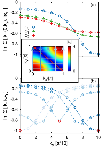
Figure 1: (Color online): Imaginary part of the self-energy $\Sigma(\mathbf{k},i\omega_{n})$ from BSS-QMC for $U=4t,$ and $\beta t=5.6$ at (a) the first three Matsubara frequencies and $k_{x}=0$; (b) at the first Matsubara frequency along the (brightness-coded) five momentum paths shown in the inset. The red points in (b) correspond to the nodal and antinodal point, which are emphasized alike in the inset by the red diagonal arrow.

The upper panel, Fig. 1(a), shows the imaginary part of the self-energy at $\mathbf{k}=(0,k_{y})$ for the first three Matsubara frequencies as a function of $k_{y}$. The variations along this high-symmetry cut through the BZ are seen to be quite significant, by a factor of about 10 at $\omega_{0}$ (circles) and still by a factor of about two at $\omega_{2}$ (diamonds). Evidently, DMFT would be completely inadequate in this respect. Only at large frequencies does the self-energy become asymptotically momentum-independent: $\Sigma(\mathbf{k},i\omega_{n})\stackrel{{\scriptstyle\omega_{n}\to\infty}}{{\longrightarrow}}U^{2}/(4i\omega_{n})$.

As seen in Fig. 1(b), the self-energy at $\Sigma(\mathbf{k},\omega_{0})$ varies strongly also along the other momentum paths indicated in the inset of Fig. 1, without an obvious structure (except for the evident mirror symmetry line $k_{x}=k_{y}$). This dependence is not particularly smooth, on the scale of our momentum grid. This indicates that approximations of the self-energy by piecewise constant patches, as usually employed in the dynamical cluster approximation (DCA) Maier et al. (2005) (on much coarser grids), may be problematic for small cluster sizes. Instead, accurate approximation schemes would have to incorporate insight in the momentum structure of $\Sigma$ [or use expansions of the self-energy that are not stepwise constant, such as the cumulant expansion (see Ref. Stanescu and Kotliar, 2006; Stanescu et al., 2006; Sakai et al., 2012; Staar et al., 2013; Sakai et al., 2009, 2016)].

III.1 Collapse of $\mathbf{k}$-dependence to a $\varepsilon_{\mathbf{k}}$-dependence

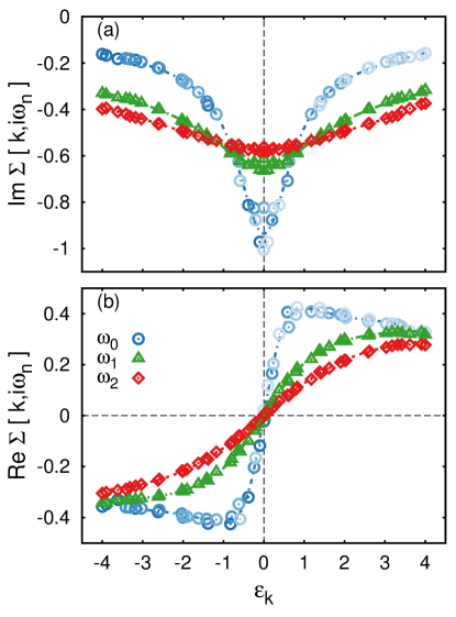
Figure 2: (Color online): Imaginary (a) and real (b) part of the self-energy $\Sigma(\mathbf{k},i\omega_{n})$ vs. the non-interacting dispersion $\varepsilon_{\mathbf{k}}$ from BSS-QMC at $U=4t$ and $\beta t=5.6$. Different $(k_{x},k_{y})$ points with the same $\varepsilon_{\mathbf{k}}$ collapse onto a single curve.

Fig. 2(a) shows Im $\Sigma(\mathbf{k},i\omega_{n})$ at the first three Matsubara frequencies plotted versus the non-interacting single-particle energy (i.e., band dispersion) $\varepsilon_{\mathbf{k}}$. Specifically, the circles in Fig. 2(a) represent all the data of Fig. 1(b) (corresponding to the lowest Matsubara frequency $\omega_{0}$). Not surprisingly, this data set is peaked for $\mathbf{k}$ at the Fermi edge, $\varepsilon_{\mathbf{k}}=0$; this is also true at the higher frequencies $\omega_{1}$ (triangles) and $\omega_{2}$ (diamonds). However, it is remarkable that each of these data sets collapse on a single line with high accuracy, with the exception of only a very narrow region around $\varepsilon_{\mathbf{k}}=0$. Global collapses are also seen in the corresponding real parts, shown in Fig. 2(b); here no low-$\varepsilon_{\mathbf{k}}$ deviations can be seen due to the linearity of Re $\Sigma$ at low $\varepsilon_{\mathbf{k}}$.

The significant momentum dependence of Im $\Sigma(\mathbf{k},\omega)$ at $\varepsilon_{\mathbf{k}}=0$, on the other hand, is nothing short of the pseudogap physics exposed in cluster extensions of DMFT,Maier et al. (2005); Civelli et al. (2005); Sakai et al. (2013) recent BSS-QMCRost et al. (2012) and D$\Gamma$A studiesSchäfer et al. (2015b): the self-energy takes different values at the Fermi surface along the nodal and antinodal directions, with variations of about $20\%$. In this respect, the nodal and antinodal points are highlighted in Fig. 1(b) as well as in the inset thereof. We learn from Fig. 2(a) that this physics is, however, narrowly confined to momentum space around the Fermi surface. Note that nodal/antinodal variations of the gap decay quickly both towards higher and lower temperatures.Rost et al. (2012) In this sense, the parameter choice of Fig. 2 ($U=4t,\beta t=5.6$) may be considered a worst case for parametrizing $\Sigma$ via $\varepsilon_{\mathbf{k}}$.

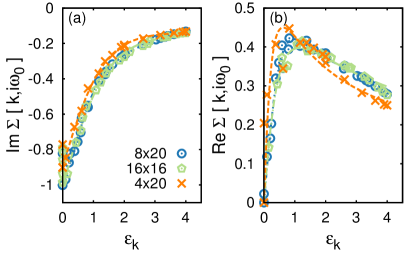
Figure 3: (Color online): Imaginary (a) and real (b) part of the self-energy $\Sigma(\mathbf{k},i\omega_{0})$ from BBS-QMC at $U=4t$ and $\beta t=5.6$. The different data points correspond to different lattice sizes and geometries.

The collapse of the self-energy $\Sigma(\mathbf{k},i\omega_{0})$ onto a single $\varepsilon_{\mathbf{k}}$-dependent $\Sigma(\varepsilon_{\mathbf{k}},i\omega_{0})$ remains unchanged when changing the cluster size in the BSS-QMC calculations. Fig. 3 compares results obtained for different system sizes and geometries. In this respect, the self-energy at $U=4t$ and $\beta t=5.6$ is shown for two lattice systems with rectangular shape, $4\times 20$ and $8\times 20$, as well as for a system with a regular square shape, having $16\times 16$ sites. We find that (i) the collapse onto a single curve (versus $\varepsilon_{\mathbf{k}}\not=0$) is better for larger systems and (ii) that, overall, the convergence seems to be quite rapid, which justifies in a qualitative way that we skipped the interpolation to an infinite system. The conclusion that our analysis is relevant in the thermodynamic limit will be further verified in Sec. III.4 by comparing BSS-QMC data, as well as the self-energy parametrization discussed in the next section, with the results obtained from $\text{D}\Gamma\text{A}$.

Very importantly, the collapse of data points with respect to $\varepsilon_{\mathbf{k}}$ is not restricted to certain interaction strengths. The self-energy in different phases (bad-metallic towards insulating) characterized by different values of $U$ is shown in Fig. 4. Compared to the case of $U=4t$ where the phase transition approximately occurs (see Ref. Rost et al., 2012), the $\mathbf{k}$ variations scale with a factor of 15 for $U=8t$; and a factor of 0.1 for $U=2t$. Despite the stronger $\varepsilon_{\mathbf{k}}$-dependence at the larger-$U$ regime, all data still collapse onto a single curve. That is, our parametrization discussed in the next section can be equally applied to both, the weak- and strong-coupling regime. It is not perturbative.

III.2 Parametrization of $\Sigma$

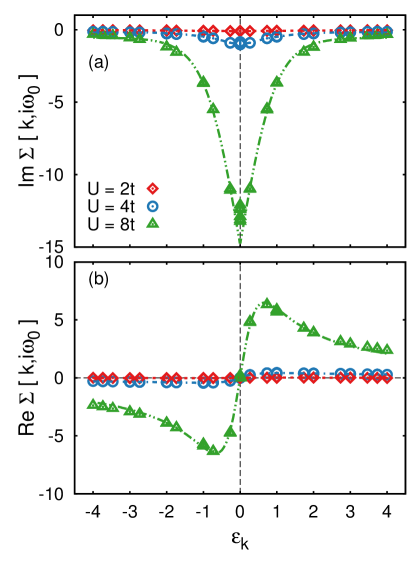
Figure 4: (Color online): Imaginary (a) and real (b) part of the self-energy $\Sigma(\mathbf{k},i\omega_{0})$ from BSS-QMC at $\beta t=5.6$ for different $U$-values.

So far, we have discussed self-energies on the imaginary frequency axis, following a common practice especially within the QMC community. While such data have the advantages of direct accessibility from (imaginary-time) QMC data and easier comparisons with literature data, real-frequency results are obviously more physically relevant and also more interesting. Such data, obtained via maximum entropy analytic continuation Jarrell and Gubernatis (1996); Bergeron and Tremblay (2015) $i\omega_{n}\rightarrow\omega$ on the level of the self-energy, are shown in Fig. 5(a) as a function of $\varepsilon_{\mathbf{k}}$ and $\omega$ at $\beta t=5.6$ and $U=4t$; the corresponding Green’s function, obtained via the Dyson equation, can be seen in Fig. 5(b). Note that these data (Im $\Sigma$, Im $G$) are, up to factors $-\pi$, spectral functions that also fully determine the corresponding real parts via Kramers-Kronig relations.

Fig. 6(a) and (b) show the same quantities but at a higher temperature $\beta t=2$.

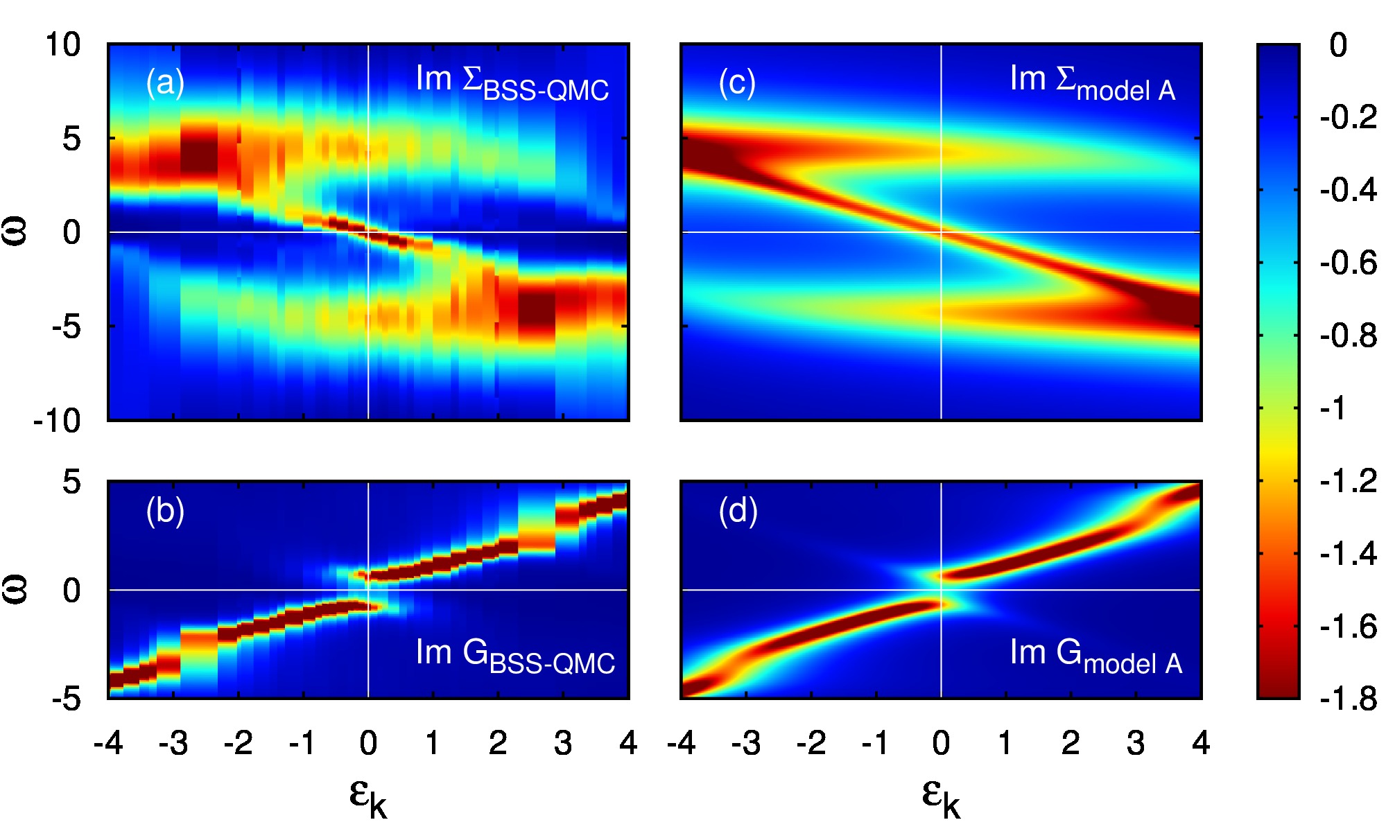
Figure 5: (Color online): Imaginary part of the self-energy $\Sigma(\varepsilon,\omega)$ and of the Green’s function $G(\varepsilon,\omega)$ at $U=4t$ and $\beta t=5.6$. (a) and (b) contain the BSS-QMC data. (c) and (d) represent continuous parametrizations, denoted in Eq. (9) and Table 1.

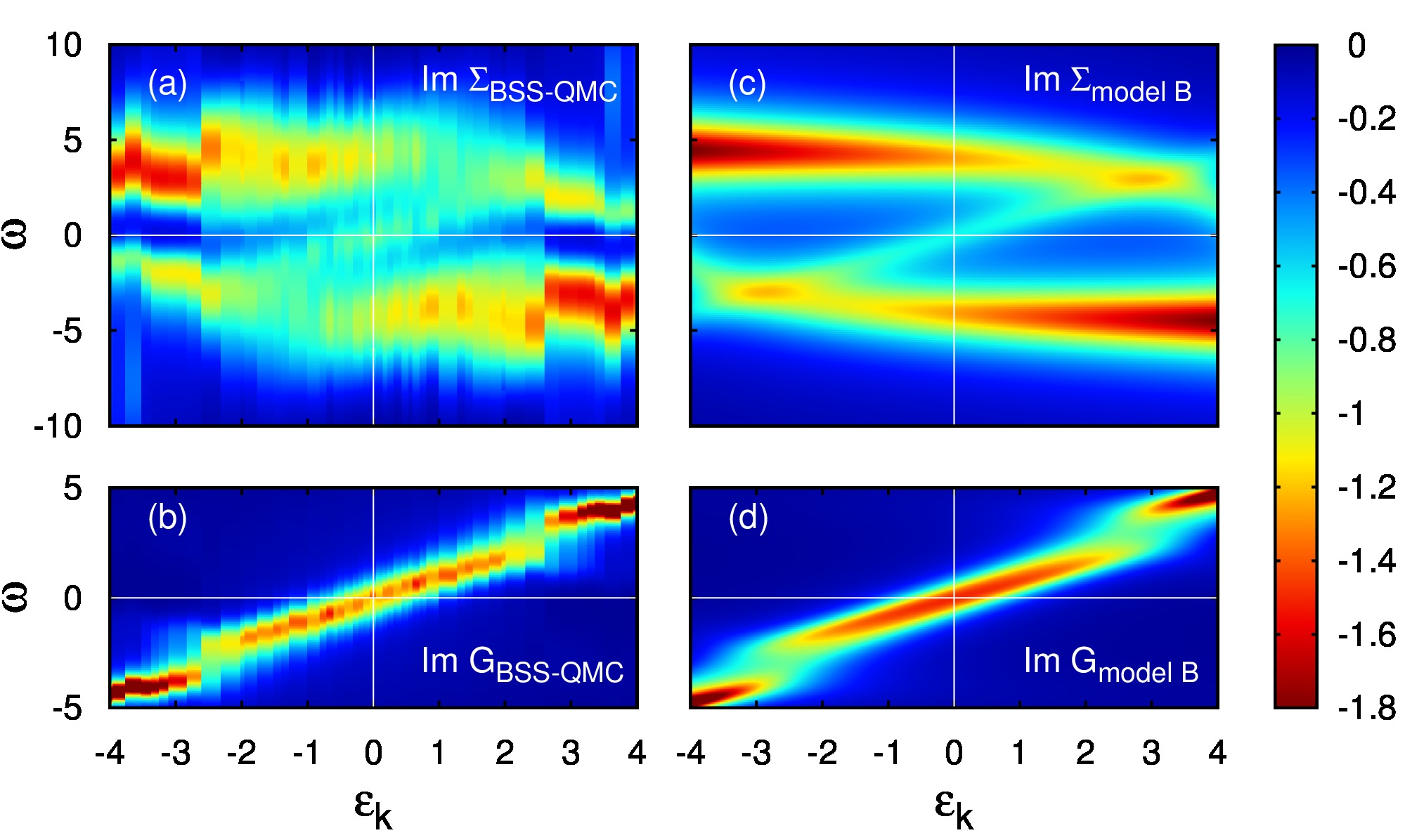
Figure 6: (Color online): Same as Fig. 5 but at a higher temperature, $\beta t=2$.

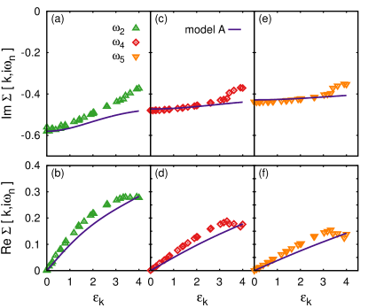
Figure 7: (Color online): The self-energy at three different (higher) Matsubara frequencies at $U=4t$ and $\beta t=5.6$. Together with the asymptotic behavior of the Matsubara self-energy, these BSS-QMC data are used to fix the model parameters in Eq. (9). The fitted parameters can be found in Table 1.

Let us now discuss the structures seen in Fig. 5(a) and Fig. 6(a). Both share a common feature, namely broad bands at high frequencies (both positive and negative), which are nearly dispersionless, i.e. with maxima fixed at $|\omega|\approx 4$. However, at a given $\varepsilon_{\mathbf{k}}$ these two dispersionless branches do not have the same weight. That is, with increasing $\varepsilon_{\mathbf{k}}$ (for $\varepsilon_{\mathbf{k}}>0$) spectral weight from the upper band ($\omega\gtrsim 2$) is shifted towards the lower band ($\omega\lesssim-2$); and vice versa for $\varepsilon_{\mathbf{k}}<0$. In addition to this high-energy structure, a strong low-energy feature with negative slope is seen at the lower temperature, in the pseudogap phase in Fig. 5(a) (precisely at $\omega=-\varepsilon_{\mathbf{k}}$). Overall, this implies a Z shaped spectral distribution of the self-energy.Sak Its low-energy part splits the (Green’s function) spectral density at $\omega\approx 0$, $\varepsilon_{\mathbf{k}}\approx 0$, i.e., introduces the pseudogap [see Fig. 5(b)].

Consequently, it is clear that the overall structure must be different at higher energies, above the pseudogap phase. However, it is surprising that the diagonal with negative unit slope, observed before, is completely absent (instead of only being weakened) in Fig. 6(a) and replaced by another diagonal with positive unit slope, i.e., with maxima at $\omega=\varepsilon_{\mathbf{k}}$. As seen in Fig. 6(b), this leads to a (Green’s function) spectral density that is only broadened in a wide frequency range, but gap-less, i.e. not split at $\omega\approx 0$.

To faithfully model the structure of the self-energy at both low and high temperatures, we consider the following parametrization,

$$\Sigma(\varepsilon,\omega)=\frac{m_{1}}{\omega+s\varepsilon+id_{1}/2}+\sum_{\alpha=\pm}\frac{m_{2}f_{\alpha}(\varepsilon)}{\omega+h_{\alpha}(\varepsilon)+id_{2}/2}\;,$$ (9)

which is obtained by decomposing the self-energy Fig. 5(a) [Fig. 6(a)] into three key features (components): the two horizontal stripes (antisymmetric in $\varepsilon$) and one sharp diagonal stripe with $s=+1$ [$s=-1$]. Each component has a density profile, which is represented by a Lorentzian function with weight $m_{1(2)}$ and width $d_{1(2)}$. For the horizontal stripes, the functions $f_{\alpha}$ and $h_{\alpha}$ describe the $\varepsilon$-dependent weight and the degree of curvature, which are taken as $f_{\pm}(\varepsilon)=1\pm b\,\varepsilon$ and $h_{\pm}(\varepsilon)=\pm 5\frac{c\pm\varepsilon}{c\pm\varepsilon+1}$.

Please note the plus and minus sign ($s=\pm 1$) in front of $\varepsilon$ in the first term of Eq. (9). Depending on the temperature, the physics is quite different as discussed in Sec. III.3 below. This is reflected in the two different signs. At low temperatures (model ASak ) we have the plus sign ($s=+1$), and at high temperature (model B) we have the minus sign ($s=-1$) for the first term of Eq. (9). To fix the parameters, we first require that the model function in Eq. (9) behaves asymptotically as $U^{2}/(4\omega)$ for $\omega\rightarrow\infty$, which reduces the independent parameters of the model function by one ($m_{1}+2m_{2}=4$). The rest of the parameters are then determined by fitting the Matsubara self-energy with a least-squares approach, as shown in Fig. 7. In Table 1, we list the different parameters of $m_{1},d_{1},d_{2},b$ and $c$, for the low- and high- temperature phases of the Hamiltonian in Eq. (1).

	$m_{1}$	$d_{1}$	$d_{2}$	$b$	$c$	$s$
model A	0.6	1.0	3.0	0.12	5.8	$+1$
model B	0.4	2.1	3.0	0.12	4.5	$-1$

Table 1: Different choices of parameters for the two models derived from Eq. (9). A and B correspond to the two best models for the self-energy at low ($\beta t=5.6$) and high temperatures ($\beta t=2$), corresponding to Fig. 5 and Fig. 6, respectively.

Despite the simple form of Eq. (9), the essential structure of the self-energy and its temperature evolution can be nicely reproduced by this parametrization. In Fig. 5(c) and (d) the self-energy and the corresponding Green’s function calculated from Eq. (9) are shown and compared to the numerically exact solution from BSS-QMC on a finite $\mathbf{k}$ grid. As we can see, model A nicely reproduces the three major structures of the self-energy, including the two horizontal stripes at high energy and the linear dependence of $\varepsilon_{\mathbf{k}}$ at low energies. As a result, the Green’s function in model A also nicely reproduces that of the BSS-QMC shown in Fig. 5(b).

At $\beta t=2$, we adopt the parameter set indicated as model B in Table 1. The comparison of model B with the BSS-QMC results is shown in Fig. 6(a)-(d). At this higher temperature, as clearly seen from the BSS-QMC results, the horizontal stripes at high energy remain, while the low-energy linear dependence on $\varepsilon_{\mathbf{k}}$ completely changes its sign as compared to Fig. 5(a), which applies a strong constraint on our model function, since a correct parametrization should also faithfully reproduce the sign change on the $\varepsilon_{\mathbf{k}}$ dependence of the self-energy at the low-energy regime. From Fig. 6, we see that model B nicely generates the correct $\varepsilon_{\mathbf{k}}$-dependence, as well as the two horizontal stripes.

III.3 Physics associated to the parametrization of $\Sigma$

In the following, we want to show that the observed structure with weakly temperature-dependent horizontal stripes and the strongly temperature-dependent linear low-energy features are natural consequences of the essential particle-hole excitations and the magnetic correlations of the Hubbard model on the square lattice. Correctly reproducing those two physical processes in our self-energy model function is a strong validation of this parametrization. Our model function, can thus be used to describe the low-energy excitations in both the charge and the spin sectors of this model.

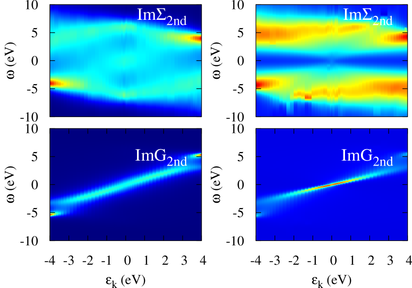
Figure 8: (Color online): Self-energy and the Green’s function calculated from second-order perturbation theory at $\beta t=1$ (left) and $\beta t=5.6$ (right) for $U=4t$.

We start from second-order perturbation theory of the self-energy, which effectively describes the motion of electrons in the background of particle-hole excitations,

$$\Sigma(\mathbf{k},\nu_{n}) = -\frac{U^{2}}{\beta^{2}N^{2}}\sum_{k^{\prime},\nu^{\prime}_{n},q,\omega_{n}}G_{\mathbf{q}-\mathbf{k},\nu_{n}-\omega_{n}}$$ (10)

$$\cdot G_{\mathbf{q}-\mathbf{k^{\prime}},\omega-\nu^{\prime}_{n}}G_{\mathbf{k^{\prime}},\nu^{\prime}_{n}}\>.$$

For the analytic continuation we utilize the Padé approximation.Vidberg and Serene (1977) Fig. 8 shows the corresponding self-energy and the Green’s function at two different temperatures $\beta t=1$ (left) and $\beta t=5.6$ (right). At both low and high temperatures, the self-energy from the second-order perturbation theory displays the two horizontal stripes at high energies. At high temperature, the same $\omega=\varepsilon_{\mathbf{k}}$ stripe as in Fig. 6(a) shows up. We thus conclude that the appearance of the horizontal stripe is due to the particle-hole excitations, which exists at both high and low temperatures.

In the low-energy regime, the linear dependence of the self-energy on $\varepsilon_{\mathbf{k}}$ disappears at low temperature, e.g., it can hardly be seen in Fig. 8 (right). But it is not replaced by a negative linear dependence of the self-energy on $\varepsilon_{\mathbf{k}}$ as observed in Fig. 5(a). This clearly tells us that the negative linear dependence in Fig. 5(a) is not due to particle-hole excitations. We find that it is, instead, an indication of the low-temperature spin-density-wave (SDW) of the 2D Hubbard model in the self-energy function. To see this, we consider a mean-field description of the Hubbard model in Eq. (1) in the presence of a SDW. The Fermi surface of the half-filled Hubbard model on the square lattice is nesting which favors the formation of a SDW with magnetic wave vector $\mathbf{Q}=(\pi,\pi)$. The corresponding magnetic Brillouin zone (MBZ) is, then, only half of the original BZ, so that the Hubbard model, Eq. (1), can be written as

$$H = \sum_{\mathbf{\tilde{k}},\sigma}\left[\varepsilon_{\mathbf{\tilde{k}}}c_{\mathbf{\tilde{k}}\sigma}^{\dagger}c_{\mathbf{\tilde{k}}\sigma}+\varepsilon_{\mathbf{\tilde{k}}+\mathbf{Q}}c_{\mathbf{\tilde{k}}\sigma}^{\dagger}c_{\mathbf{\tilde{k}}+\mathbf{Q}\sigma}\right]$$ (11)

$$+U\sum_{\mathbf{k},\mathbf{k^{\prime}}}c_{\mathbf{k}\uparrow}^{\dagger}c_{\mathbf{k}+\mathbf{Q}\uparrow}c_{\mathbf{k^{\prime}}\downarrow}^{\dagger}c_{\mathbf{k^{\prime}}+\mathbf{Q}\downarrow}\>,$$

where the sum over $\mathbf{\tilde{k}}$ is restricted to the MBZ, whereas the sum over $\mathbf{k}$ is in the original BZ. After defining a mean-field order parameter for the SDW

$$\Delta=U\sum_{\mathbf{k}}\sigma c_{\mathbf{k}\sigma}^{\dagger}c_{\mathbf{k}+\mathbf{Q}\sigma}\>,$$ (12)

the mean-field Hamiltonian can be written as

$$H = \sum_{\mathbf{\tilde{k}},\sigma}\left[\varepsilon_{\mathbf{\tilde{k}}}c_{\mathbf{\tilde{k}}\sigma}^{\dagger}c_{\mathbf{\tilde{k}}\sigma}+\varepsilon_{\mathbf{\tilde{k}}+\mathbf{Q}}c_{\mathbf{\tilde{k}}\sigma}^{\dagger}c_{\mathbf{\tilde{k}}+\mathbf{Q}\sigma}\right]$$ (13)

$$-\Delta\sum_{\mathbf{k}}\left[c_{\mathbf{k}\uparrow}^{\dagger}c_{\mathbf{k}+\mathbf{Q}\uparrow}-c_{\mathbf{k}+\mathbf{Q}\downarrow}^{\dagger}c_{\mathbf{k}\downarrow}\right]\;.$$

If we restrict the sum over $\mathbf{k}$ in the second term to be also inside the MBZ and consider only one spin component, we have the following compact form of the mean-field Hamiltonian,

$$H=\sum_{\mathbf{\tilde{k}}}\left(c_{\mathbf{\tilde{k}}}^{\dagger},c_{\mathbf{\tilde{k}}+\mathbf{Q}}^{\dagger}\right)\begin{pmatrix}\varepsilon_{\mathbf{\tilde{k}}}&-\Delta\cr-\Delta&\varepsilon_{\mathbf{\tilde{k}}+\mathbf{Q}}\end{pmatrix}\begin{pmatrix}c_{\mathbf{\tilde{k}}}\cr c_{\mathbf{\tilde{k}}+\mathbf{Q}}\end{pmatrix}\;,$$ (14)

from which the single-particle Green’s function can be easily calculated as

$$G_{\mathbf{\tilde{k}},\omega} = \frac{\omega-\varepsilon_{\mathbf{\tilde{k}}+\mathbf{Q}}}{(\omega-\varepsilon_{\mathbf{\tilde{k}}})(\omega-\varepsilon_{\mathbf{\tilde{k}}+\mathbf{Q}})-\Delta^{2}}$$ (15)

$$= \frac{1}{\omega-\varepsilon_{\mathbf{\tilde{k}}}-\frac{\Delta^{2}}{\omega-\varepsilon_{\mathbf{\tilde{k}}+\mathbf{Q}}}}\;.$$

Thus, the self-energy of the Hubbard model from the SDW mean-field theory is

$$\Sigma(\mathbf{\tilde{k}},\omega)=\frac{\Delta^{2}}{\omega-\varepsilon_{\mathbf{\tilde{k}}+\mathbf{Q}}}=\frac{\Delta^{2}}{\omega+\varepsilon_{\mathbf{\tilde{k}}}}\;,$$ (16)

which leads to the strong negative linear-dependence $\omega=-\varepsilon_{\mathbf{k}}$ at low energies. Since second-order perturbation theory does not include the magnetic correlations of the system, it is not surprising that, at low temperature, the self-energy calculated from it does not contain such a negative linear $\varepsilon_{\mathbf{\tilde{k}}}$-dependence. We want to note that, despite the simple form of our model function in Eq. (9), it correctly describes the magnetic correlations which only appear at higher orders of perturbation theory. Our model function can then be used to describe the competition between the charge and the spin degrees of freedom which becomes important when the temperature decreases.

In Eq. (16), we have used the fact that $\varepsilon_{\mathbf{\tilde{k}}+\mathbf{Q}}=-\varepsilon_{\mathbf{\tilde{k}}}$, which holds for a square lattice where $\mathbf{Q}\approx(\pi,\pi)$. For general lattices, $\varepsilon_{\mathbf{k}+\mathbf{Q}}$ is not uniquely related to $\varepsilon_{\mathbf{k}}$. One might expect that this leads to a somewhat more complicated self-energy parametrization: $\Sigma(\mathbf{k},\omega)\to\Sigma(\varepsilon_{\mathbf{k}},\varepsilon_{\mathbf{k}+\mathbf{Q}},\omega)$.

III.4 Comparison to D$\Gamma$A

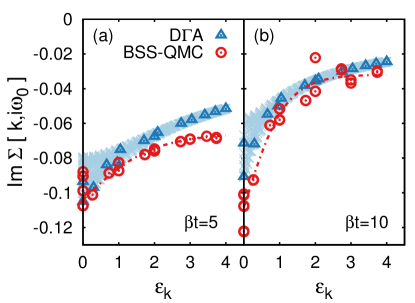
Figure 9: (Color online): Imaginary part of the self-energy $\Sigma(\mathbf{k},i\omega_{0})$ for $U=2t$ and two different temperatures: (a) $\beta t=5$ and (b) $\beta t=10$. The (light blue) continuum of data points represent all different $\text{D}\Gamma\text{A}$ momenta for a given $\varepsilon_{\mathbf{k}}$. For a better comparison of $\text{D}\Gamma\text{A}$ with BSS-QMC, we highlighted data points in the $\text{D}\Gamma\text{A}$ calculation (dark-blue triangles) that correspond to the BSS-QMC data (red circles) with similar $\mathbf{k}$-points.

The self-energy parametrization proposed in Eq. (9) is based on the large-scale simulation of the BSS-QMC. By comparing the results for different sizes of clusters, we have shown that the collapses of the self-energy onto $\Sigma(\varepsilon_{\mathbf{k}},\omega)$ in BSS-QMC are observed for all sufficiently large cluster sizes. In this section, we further confirm that our parametrization of the self-energy via the non-interacting dispersion also holds in the thermodynamic limit (including spatial correlations on every length scale). Toward that end, we perform calculations by means of the D$\Gamma$A (introduced in Sec. II.2).

Fig. 9 presents the imaginary part of $\Sigma(\varepsilon_{\mathbf{k}},i\omega_{0})$ for $U=2t$. The light blue data points in the background correspond to the data at all available $\mathbf{k}$-points of the D$\Gamma$A calculation. Due to a higher resolution in $\mathbf{k}$-space for the $\text{D}\Gamma\text{A}$ self-energy, we have more $\mathbf{k}$-points within this method. Those $\mathbf{k}$-points, similar to those of the BSS-QMC calculation (dotted circles), are represented by dark-blue triangles. The absolute deviations of the two methods might be due to diagrams beyond ladder D$\Gamma$A or due to the BSS-QMC coarse graining. Nevertheless, the collapse of $\Sigma(\varepsilon_{\mathbf{k}},i\omega_{0})$ away from the Fermi energy $\varepsilon_{\mathbf{k}}=0$ survives in the thermodynamic limit. That is, the light blue triangles essentially collapse onto a single line with only minor deviations. In particular, the behavior of $\Sigma(\varepsilon_{\mathbf{k}},i\omega_{0})$ in D$\Gamma$A resembles that of BSS-QMC in view of the fact that leaving the Fermi edge $\varepsilon_{\mathbf{k}}=0$, the spread of the data points gets drastically diminished. Again, the relatively big spread at the Fermi edge of the D$\Gamma$A self-energy can be explained physically by the onset of the opening of a pseudogap in this region of the (D$\Gamma$A) phase diagramKatanin et al. (2009); Schäfer et al. (2015b, 2016). For $U=2t$, the pseudogap phase is relatively small from $T=0.05t$ to $T=0.07t$ (in our units). That is, at $T=\frac{1}{\beta}=\frac{t}{5}=0.2t$ the pseudogap has not opened yet but there is already a large scattering; Im $\Sigma$ at $(\pi,0)$ is already large.Schäfer et al. (2016) Reducing the temperature to $T=0.1t$, the spread at the Fermi level increases further. However, the collapse away from the Fermi edge persists [see Fig. 9(b)].

Leaving the vicinity of the Fermi edge by choosing a finite Matsubara frequency, the collapse becomes even more drastic as can be seen in the first row of Fig. 10, where the imaginary part of $\Sigma(\varepsilon_{\mathbf{k}},i\omega_{n})$ is plotted for $U=4t$ and $\beta{t}=2$ for the first [Fig. 10(a)] and second [Fig. 10(b)] Matsubara frequency respectively. One can observe that especially for $\varepsilon_{\mathbf{k}}\rightarrow{0}$, the spread of $\text{Im }\Sigma(\varepsilon_{\mathbf{k}},i\omega_{1})$ is much smaller than that of $\text{Im }\Sigma(\varepsilon_{\mathbf{k}},i\omega_{0})$, again a feature signaling the onset of the pseudogap phase.  Additionally, the collapse of the real part of the self-energy [see the lower row of Fig. 10(b)] supports the significance of the energy-parametrization of the self-energy.

Concluding this comparison, the switch from the finite-size cluster in BSS-QMC to the thermodynamic limit in D$\Gamma$A does not seem to have any influence on the qualitative phenomenon of the collapse of the self-energy parametrization.

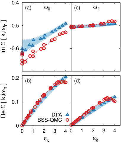
Figure 10: (Color online): The self-energy for $U=4t$, $\beta t=2$ and the first (left) and second (right) Matsubara frequencies comparing BSS-QMC (red circles) and $\text{D}\Gamma\text{A}$ (light blue; and dark blue triangles for similar momenta as the red circles).

III.5 Anisotropic Case

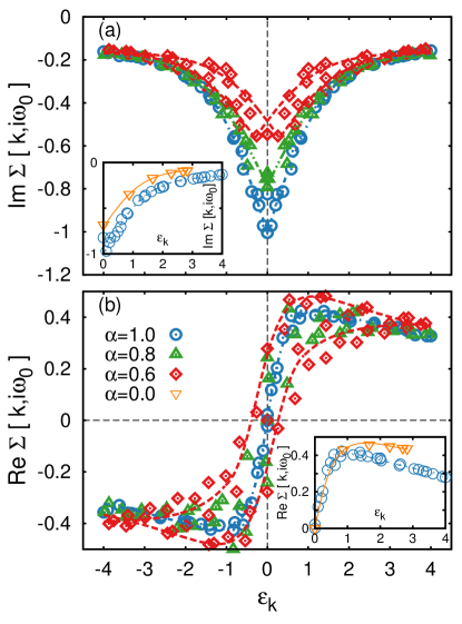
Figure 11: (Color online): Imaginary (a) and real (b) part of the self-energy $\Sigma(\mathbf{k},i\omega_{0})$ from BSS-QMC at $U=4t$ and $\beta t=5.6$ but for various degrees of anisotropies $\alpha$. Green and red lines are guides to the eye only, not fits to the parametrization model as in the other figures.

So far, we have considered the Hubbard model on an isotropic lattice. We found that the two momentum degrees of freedom appearing (besides the frequency) as variables of the self-energy can be replaced by one energy-like variable with good accuracy and for almost all $\mathbf{k}$: $\Sigma(\mathbf{k},\omega)\equiv\Sigma(\varepsilon_{\mathbf{k}},\omega)$. It is easy to see that such an replacement would be exact (globally) in one dimension (for nearest neighbor hopping): then, there is only one momentum variable $k_{x}$. Since $\varepsilon_{k_{x}}$ increases monotonously with $k_{x}\in[0,\pi]$ (in the case of hopping only between nearest neighbors), and $\pm k_{x}$ are equivalent by symmetry, there exists a unique mapping $\mathbf{k}\leftrightarrow\varepsilon_{\mathbf{k}}$ in one dimension (within the reduced BZ).

The question to be addressed in this section is, whether the parametrization of $\Sigma$ via $\varepsilon_{\mathbf{k}}$ works also in the crossover region between these limits. For this purpose, we consider the anisotropic two-dimensional lattice with a hopping ratio $0\leq\alpha=t_{x}/t_{y}\leq 1$; in order to keep the kinetic energy scale $(2t_{x}^{2}+2t_{y}^{2})^{1/2}=2t$ fixed, we set $t_{y}=\sqrt{2t^{2}/(\alpha^{2}+1)}$ (and $t_{x}=\alpha\,t_{y}$).

Corresponding BSS-QMC results are shown for $\alpha=1$ (the isotropic case considered before), $\alpha=0.8$, and $\alpha=0.6$ in the main panels of Fig. 11. It is immediately seen that the spread of each data set, associated with an incomplete collapse, increases rapidly with increasing anisotropy, both in the real and imaginary parts of the self-energy. Only in the one-dimensional limit ($\alpha=0$), shown in the insets, do the data fall, again, onto single curves (which are remarkably similar to their two-dimensional counterparts).

Note that Im $\Sigma$ still shows a reasonably good collapse at $\alpha=0.8$ [triangles in Fig. 11(a)], while the deviations from a common curve are nearly an order of magnitude larger for Re $\Sigma$ [triangles in Fig. 11(b)]. This distinction already hints at the physical reason why a parametrization of the self-energy in terms of the free dispersion cannot work in full generality: In the absence of sufficient symmetries, interactions modify the Fermi surface (while keeping its volume constant at least in the Fermi liquid regime). This direction-dependent shift is encoded, to first order, in Re $\Sigma(\mathbf{k},\omega)\large|_{\varepsilon_{\mathbf{k}}=0,\omega=0}$, which would vanish exactly in a parametrization via $\varepsilon_{\mathbf{k}}$.

Thus, the analysis of this paper seems to apply directly only to the case of very weak (or very strong) anisotropies. It remains to be seen whether the results of a parametrization such as that performed in Sec. III.3 could be useful also in the cases in which the true self-energy does not have this form (as for $\alpha=0.6$) or if the analysis can be extended in order to incorporate Fermi surface deformation.

III.6 Doping

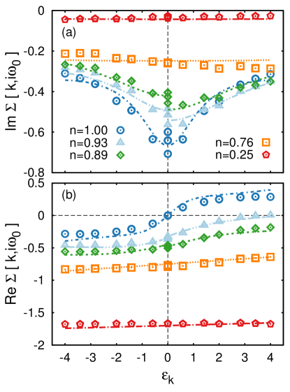
Figure 12: (Color online): Imaginary (a) and real (b) part of the self-energy $\Sigma(\mathbf{k},i\omega_{0})$ from BSS-QMC at $U=4t$, $\beta t=3.6$ and $L=8\times 8$ for doped systems.

So far, we have considered the Hubbard model at half-filling ($n=1$). Similar insights with respect to the structure of the self-energy would be even more welcome for doped systems, as these are directly relevant for high-temperature superconductivity, i.e., physically even more interesting, and also particularly challenging. However, as BSS-QMC simulations then suffer from the notorious “minus-sign” problem, due to the lack of particle-hole symmetry, the numerical effort is much greater (at fixed statistical error). Consequently, we need to reduce the lattice size to $8\times 8$ in our calculations. We should stress, as a caveat, that the resulting reduction in the number of inequivalent $\mathbf{k}$ points implies a much sparser $\varepsilon$ grid which makes it more difficult to check for a collapse of $\Sigma$ versus $\varepsilon_{\mathbf{k}}$.

Away from half-filling ($n\neq 1$), the self-energy becomes asymmetric with respect to $\varepsilon_{\mathbf{k}}=0$, as shown in Fig. 12 for the isotropic 2D case. In this figure, we show the (a) imaginary and the (b) real part of the self-energy at five different doping levels characterized by the different values of the electronic density $n$. Symbols in Fig. 12 correspond to the BSS-QMC data, and the dotted and dashed lines are obtained by fitting these data with model A in Table 1.

The first observation for the doped case is that the spread of the self-energy (in the imaginary part) remains at $\varepsilon_{\mathbf{k}}=0$ and quickly disappears by increasing doping. Thus, for a given doping level the self-energy again collapses onto a single curve, which makes a parametrization possible, as in the half-filled case. Note that in order to fit the data in Fig. 12, in addition to model A, we added a constant (with imaginary and real parts) and we took a different fit model for $\varepsilon_{\mathbf{k}}>0$ and $\varepsilon_{\mathbf{k}}<0$. This way, model A still nicely describes the curvature of the BSS-QMC self-energy.

For the doped case, we observe deviations from model A [in its original form presented in Eq. (9)], but the general form $\Sigma(\mathbf{k},\omega)\to\Sigma(\varepsilon_{\mathbf{k}},\omega)$ still holds. Again (as in the anisotropic case), the deviations from a smooth dependence of $\Sigma$ on $\varepsilon_{\mathbf{k}}$ can be understood as resulting from deformations of the Fermi surface.

IV Conclusion & Outlook

Despite the fundamental importance of the self-energy $\Sigma(\mathbf{k},\omega)$ within the Hubbard model, little was known about its momentum-frequency structure in the most interesting and challenging cases of $d=2$ and $d=3$ spatial dimensions. One complicating factor in earlier analyses was certainly the high dimensionality $(d+1)$ of the momentum-frequency parameter space, making a full global visualization impossible already in two spatial dimensions.

This situation is changed by our finding that the momentum dependence of the self-energy reduces, with remarkably high precision and scope, to a dependence on the non-interacting energy $\varepsilon_{\mathbf{k}}$ at each point in momentum space, i.e. $\Sigma(\mathbf{k},\omega)\to\Sigma(\varepsilon,\omega)$ on a square lattice, where $\varepsilon=\varepsilon_{\mathbf{k}}$. Thereby, we could not only fully visualize the numerically obtained self-energy in the density plots of Fig. 5(a) and Fig. 6(a) at temperatures in and above the pseudogap phase, respectively (note that these spectral data also determine Re $\Sigma$), but we could also derive complete parametrizations that highlight the interesting physics previously hidden in this system. We could trace back the strong Z shaped low-$T$ structure to the generation of (self-energy) spectral density at $\omega=\varepsilon_{\mathbf{k}+\mathbf{Q}}=-\varepsilon_{\mathbf{k}}$ by antiferromagnetic fluctuations. For other lattices $\varepsilon_{\mathbf{k}+\mathbf{Q}}\neq-\varepsilon_{\mathbf{k}}$, suggesting a parametrization $\Sigma(\varepsilon_{\mathbf{k}},\varepsilon_{\mathbf{k}+\mathbf{Q}},\omega)$.

Given this explanation, one might have expected the spectral features to decay only weakly towards higher temperatures, similarly to the nearest-neighbor spin correlation function. However, the higher-$T$ results completely lack any (lower-energy) features at $\omega=-\varepsilon_{\mathbf{k}}$, and they show, instead, significant contributions at $\omega=\varepsilon_{\mathbf{k}}$, leading to an overall Z-shaped structure that appears also in second-order perturbation theory.

Note that our ansatz for the self-energy is the most general one consistent with the functional form of the Green’s function $G\equiv G(\varepsilon_{\mathbf{k}},\omega)$ that is valid also within DMFT. However, it is clear that DMFT taps only a very limited subspace of this class of Green’s functions.

Limitations of the ansatz $\Sigma\equiv\Sigma(\varepsilon_{\mathbf{k}},\omega)$ become apparent both directly at the Fermi surface in the pseudogap phase and, more globally, in the case of strongly anisotropic lattices. In the former case, the breakdown is inevitable, since an anisotropic gap cannot possibly be described by a self-energy that is constant along the Fermi surface (at each fixed frequency). This also holds at temperatures somewhat above the pseudogap phase, where the scattering rates at the nodal and antinodal point of the Fermi surface are very different. In the latter case, the physics behind the deviation is the deformation of the Fermi surface. For the doped square lattice the general form $\Sigma(\mathbf{k},\omega)\to\Sigma(\varepsilon_{\mathbf{k}},\omega)$ is still applicable, albeit our model parametrization does not work any longer.

Another fascinating feature of our ansatz is that it allows for a direct comparison of self-energies associated with systems of different spatial dimensionality (such as those shown in the insets of Fig. 11), as the parameter space is always two-dimensional. In fact, it is reasonable to assume that the analysis of this paper would work even better (with even greater reductions of the complexity) for cubic lattices, i.e. in three dimensions. However, a reliable verification would require quite large lattices (at still high numerical precision) and it was, therefore, beyond the scope of this work.

V acknowledgment

We acknowledge financial support through the DFG research unit FOR 1346 (PP, DR, NB) and the European Research Council under the European Union’s Seventh Framework Program (FP/2007-2013)/ERC through grant agreement n. 306447 (PP, GL, KH); and support from the Austrian Science Fund (FWF) through the doctoral school “Building Solids for Function” (FWF W1243) and project I-610 (TS). Calculations have been done in part on the Vienna Scientific Cluster (VSC).

References

- Mahan (2013) G. D. Mahan, Many-particle physics (Springer Science & Business Media, 2013).
- Negele and Orland (1988) J. W. Negele and H. Orland, Quantum many-particle systems, Vol. 200 (Addison-Wesley New York, 1988).
- Landau (1957) L. D. Landau, “The theory of a Fermi liquid,” Sov. Phys. JETP 3, 920–925 (1957).
- Mott (1949) N. F. Mott, “The basis of the electron theory of metals, with special reference to the transition metals,” Proc. Phys. Soc. Sec. A 62, 416 (1949).
- Mott (1968) N. F. Mott, “Metal-insulator transition,” Rev. Mod. Phys. 40, 677–683 (1968).
- Gebhard (1997) F. Gebhard, The Mott metal-insulator transition, Springer Tracts in Modern Physics, Vol. 137 (Springer-Verlag Berlin Heidelberg, 1997).
- Stewart (2001) G. R. Stewart, “Non-Fermi-liquid behavior in - and -electron metals,” Rev. Mod. Phys. 73, 797–855 (2001).
- Schulz (1954) H. J. Schulz, “Fermi liquids and non-Fermi liquids,” in Proceedings of Les Houches Summer School LXI, edited by E. Akkermans, G. Montambaux, J. Pichard, and J. Zinn-Justin (Elsevier, Amsterdam, 1954) p. 533.
- Nekrasov et al. (2006) I. A. Nekrasov, K. Held, G. Keller, D. E. Kondakov, T. Pruschke, M. Kollar, O. K. Andersen, V. I. Anisimov, and D. Vollhardt, “Momentum-resolved spectral functions of calculated by ,” Phys. Rev. B 73, 155112 (2006).
- Byczuk et al. (2007) K. Byczuk, M. Kollar, K. Held, Y.-F. Yang, I. A. Nekrasov, T. Pruschke, and D. Vollhardt, “Kinks in the dispersion of strongly correlated electrons,” Nat. Phys. 3, 168 – 171 (2007).
- Held et al. (2013) K. Held, R. Peters, and A. Toschi, “Poor man’s understanding of kinks originating from strong electronic correlations,” Phys. Rev. Lett. 110, 246402 (2013).
- Kotliar and Vollhardt (2004) G. Kotliar and D. Vollhardt, “Strongly correlated materials: Insights from dynamical mean-field theory,” Physics Today 57, 53–60 (2004).
- Georges et al. (1996) A. Georges, G. Kotliar, W. Krauth, and M. J. Rozenberg, “Dynamical mean-field theory of strongly correlated fermion systems and the limit of infinite dimensions,” Rev. Mod. Phys. 68, 13–125 (1996).
- Metzner and Vollhardt (1989) W. Metzner and D. Vollhardt, “Correlated lattice fermions in dimensions,” Phys. Rev. Lett. 62, 324–327 (1989).
- Schäfer et al. (2015a) T. Schäfer, A. Toschi, and J. M. Tomczak, “Separability of dynamical and nonlocal correlations in three dimensions,” Phys. Rev. B 91, 121107 (2015a).
- Tomczak et al. (2012) J. M. Tomczak, M. van Schilfgaarde, and G. Kotliar, “Many-body effects in iron pnictides and chalcogenides: Nonlocal versus dynamic origin of effective masses,” Phys. Rev. Lett. 109, 237010 (2012).
- Taranto et al. (2013) C. Taranto, M. Kaltak, N. Parragh, G. Sangiovanni, G. Kresse, A. Toschi, and K. Held, “Comparing quasiparticle GW+DMFT and LDA+DMFT for the test bed material ,” Phys. Rev. B 88, 165119 (2013).
- Tomczak et al. (2014) J. M. Tomczak, M. Casula, T. Miyake, and S. Biermann, “Asymmetry in band widening and quasiparticle lifetimes in : Competition between screened exchange and local correlations from combined GW and dynamical mean-field theory GW + ,” Phys. Rev. B 90, 165138 (2014).
- Rubtsov et al. (2008) A. N. Rubtsov, M. I. Katsnelson, and A. I. Lichtenstein, “Dual fermion approach to nonlocal correlations in the Hubbard model,” Phys. Rev. B 77, 033101 (2008).
- Rohringer et al. (2013) G. Rohringer, A. Toschi, H. Hafermann, K. Held, V. I. Anisimov, and A. A. Katanin, “One-particle irreducible functional approach: A route to diagrammatic extensions of the dynamical mean-field theory,” Phys. Rev. B 88, 115112 (2013).
- Li (2015) G. Li, “Hidden physics in the dual-fermion approach: A special case of a nonlocal expansion scheme,” Phys. Rev. B 91, 165134 (2015).
- Blankenbecler et al. (1981) R. Blankenbecler, D. J. Scalapino, and R. L. Sugar, “Monte Carlo calculations of coupled boson-fermion systems. I,” Phys. Rev. D 24, 2278–2286 (1981).
- Toschi et al. (2007) A. Toschi, A. A. Katanin, and K. Held, “Dynamical vertex approximation: A step beyond dynamical mean-field theory,” Phys. Rev. B 75, 045118 (2007).
- Katanin et al. (2009) A. A. Katanin, A. Toschi, and K. Held, “Comparing pertinent effects of antiferromagnetic fluctuations in the two- and three-dimensional Hubbard model,” Phys. Rev. B 80, 075104 (2009).
- Hettler et al. (1998) M. H. Hettler, A. N. Tahvildar-Zadeh, M. Jarrell, T. Pruschke, and H. R. Krishnamurthy, “Nonlocal dynamical correlations of strongly interacting electron systems,” Phys. Rev. B 58, R7475–R7479 (1998).
- Kotliar et al. (2001) G. Kotliar, S. Y. Savrasov, G. Pálsson, and G. Biroli, “Cellular dynamical mean field approach to strongly correlated systems,” Phys. Rev. Lett. 87, 186401 (2001).
- Lichtenstein and Katsnelson (2000) A. I. Lichtenstein and M. I. Katsnelson, “Antiferromagnetism and d-wave superconductivity in cuprates: A cluster dynamical mean-field theory,” Phys. Rev. B 62, R9283–R9286 (2000).
- Hettler et al. (2000) M. H. Hettler, M. Mukherjee, M. Jarrell, and H. R. Krishnamurthy, “Dynamical cluster approximation: Nonlocal dynamics of correlated electron systems,” Phys. Rev. B 61, 12739–12756 (2000).
- Jarrell et al. (2001) M. Jarrell, T. Maier, C. Huscroft, and S. Moukouri, “Quantum Monte Carlo algorithm for nonlocal corrections to the dynamical mean-field approximation,” Phys. Rev. B 64, 195130 (2001).
- Maier et al. (2005) T. Maier, M. Jarrell, T. Pruschke, and M. H. Hettler, “Quantum cluster theories,” Rev. Mod. Phys. 77, 1027–1080 (2005).
- Gull et al. (2011) E. Gull, P. Staar, S. Fuchs, P. Nukala, M. S. Summers, T. Pruschke, T. C. Schulthess, and T. Maier, “Submatrix updates for the continuous-time auxiliary-field algorithm,” Phys. Rev. B 83, 075122 (2011).
- LeBlanc et al. (2015) J. P. F. LeBlanc, A. E. Antipov, F. Becca, I. W. Bulik, G. K.-L. Chan, C.-M. Chung, Y. Deng, M. Ferrero, T. M. Henderson, C. A. Jiménez-Hoyos, E. Kozik, X.-W. Liu, A. J. Millis, N. V. Prokof’ev, M. Qin, G. E. Scuseria, H. Shi, B. V. Svistunov, L. F. Tocchio, I. S. Tupitsyn, S. R. White, S. Zhang, B.-X. Zheng, Z. Zhu, and E. Gull (Simons Collaboration on the Many-Electron Problem), “Solutions of the two-dimensional Hubbard model: Benchmarks and results from a wide range of numerical algorithms,” Phys. Rev. X 5, 041041 (2015).
- Schäfer et al. (2015b) T. Schäfer, F. Geles, D. Rost, G. Rohringer, E. Arrigoni, K. Held, N. Blümer, M. Aichhorn, and A. Toschi, “Fate of the false Mott-Hubbard transition in two dimensions,” Phys. Rev. B 91, 125109 (2015b).
- Suzuki (1976) M. Suzuki, “Relationship between -dimensional quantal spin systems and -dimensional Ising systems: Equivalence, critical exponents and systematic approximants of the partition function and spin correlations,” Progr. Theor. Phys. 56, 1454–1469 (1976).
- Trotter (1959) H. F. Trotter, “On the product of semi-groups of operators,” Proc. Amer. Math. Soc. 10 , 545–551 (1959).
- Stratonovich (1957) R. L. Stratonovich, “On a method of calculating quantum distribution functions,” Soviet Physics Doklady 2, 416 (1957).
- Hubbard (1959) J. Hubbard, “Calculation of partition functions,” Phys. Rev. Lett. 3, 77–78 (1959).
- Hirsch (1983) J. E. Hirsch, “Discrete Hubbard-Stratonovich transformation for fermion lattice models,” Phys. Rev. B 28, 4059–4061 (1983).
- Gorelik and Blümer (2009) E. V. Gorelik and N. Blümer, “Mott transitions in ternary flavor mixtures of ultracold fermions on optical lattices,” Phys. Rev. A 80, 051602 (2009).
- Rost et al. (2013) D. Rost, F. Assaad, and N. Blümer, “Quasi-continuous-time impurity solver for the dynamical mean-field theory with linear scaling in the inverse temperature,” Phys. Rev. E 87, 053305 (2013).
- Assaad and Evertz (2008) F. F. Assaad and H. G. Evertz, World-line and determinantal quantum Monte Carlo methods for spins, phonons and electrons (Springer, 2008).
- Chang et al. (2015) C.-C. Chang, S. Gogolenko, J. Perez, Z. Bai, and R. T. Scalettar, “Recent advances in determinant quantum Monte Carlo,” Philos. Mag. 95, 1260–1281 (2015).
- Kusunose (2006) H. Kusunose, “Influence of spatial correlations in strongly correlated electron systems: Extension to dynamical mean field approximation,” J. Phys. Soc. Jpn 75, 054713 (2006).
- Hafermann et al. (2008) H. Hafermann, S. Brener, A. Rubtsov, M. Katsnelson, and A. Lichtenstein, “Cluster dual fermion approach to nonlocal correlations,” JETP Lett. 86, 677–682 (2008).
- Taranto et al. (2014) C. Taranto, S. Andergassen, J. Bauer, K. Held, A. Katanin, W. Metzner, G. Rohringer, and A. Toschi, “From infinite to two dimensions through the functional renormalization group,” Phys. Rev. Lett. 112, 196402 (2014).
- Ayral and Parcollet (2015) T. Ayral and O. Parcollet, “Mott physics and spin fluctuations: a unified framework,” Phys Rev. B 92, 115109 (2015).
- Kitatani et al. (2015) M. Kitatani, N. Tsuji, and H. Aoki, “FLEX+DMFT approach to the -wave superconducting phase diagram of the two-dimensional Hubbard model,” Phys. Rev. B 92, 085104 (2015).
- Valli et al. (2015) A. Valli, T. Schäfer, P. Thunström, G. Rohringer, S. Andergassen, G. Sangiovanni, K. Held, and A. Toschi, “Dynamical vertex approximation in its parquet implementation: Application to Hubbard nanorings,” Phys. Rev. B 91, 115115 (2015).
- Li et al. (2016) G. Li, N. Wentzell, P. Pudleiner, P. Thunström, and K. Held, “Efficient implementation of the parquet equations: Role of the reducible vertex function and its kernel approximation,” Phys. Rev. B 93, 165103 (2016).
- Held et al. (2011) K. Held, C. Taranto, G. Rohringer, and A. Toschi, “Hedin equations, GW, GW+DMFT, and all that,” in The LDA+DMFT Approach to Strongly Correlated Materials - Lecture Notes of the Autumn School 2011 Hands-on LDA+DMFT, Reihe Modeling and Simulation, Vol. 1, edited by E. Pavarini, E. Koch, D. Vollhardt, and A. Lichtenstein (Forschungszentrum Jülich, 2011).
- Rohringer et al. (2011) G. Rohringer, A. Toschi, A. Katanin, and K. Held, “Critical properties of the half-filled Hubbard model in three dimensions,” Phys. Rev. Lett. 107, 256402 (2011).
- Note (1) For the properties of the local vertices see Ref. \rev@citealpnumPhysRevB.86.125114, PhysRevLett.110.246405.
- Stanescu and Kotliar (2006) T. D. Stanescu and G. Kotliar, “Fermi arcs and hidden zeros of the Green function in the pseudogap state,” Phys. Rev. B 74, 125110 (2006).
- Stanescu et al. (2006) T. D. Stanescu, M. Civelli, K. Haule, and G. Kotliar, “A cellular dynamical mean field theory approach to Mottness,” Ann. Phys. 321, 1682 – 1715 (2006), July 2006 Special Issue.
- Sakai et al. (2012) S. Sakai, G. Sangiovanni, M. Civelli, Y. Motome, K. Held, and M. Imada, “Cluster-size dependence in cellular dynamical mean-field theory,” Phys. Rev. B 85, 035102 (2012).
- Staar et al. (2013) P. Staar, T. Maier, and T. C. Schulthess, “Dynamical cluster approximation with continuous lattice self-energy,” Phys. Rev. B 88, 115101 (2013).
- Sakai et al. (2009) S. Sakai, Y. Motome, and M. Imada, “Evolution of electronic structure of doped Mott insulators: Reconstruction of poles and zeros of Green’s function,” Phys. Rev. Lett. 102, 056404 (2009).
- Sakai et al. (2016) S. Sakai, M. Civelli, and M. Imada, “Hidden fermionic excitation boosting high-temperature superconductivity in cuprates,” Phys. Rev. Lett. 116, 057003 (2016).
- Civelli et al. (2005) M. Civelli, M. Capone, S. S. Kancharla, O. Parcollet, and G. Kotliar, “Dynamical breakup of the Fermi surface in a doped Mott insulator,” Phys. Rev. Lett. 95, 106402 (2005).
- Sakai et al. (2013) S. Sakai, S. Blanc, M. Civelli, Y. Gallais, M. Cazayous, M.-A. Méasson, J. S. Wen, Z. J. Xu, G. D. Gu, G. Sangiovanni, Y. Motome, K. Held, A. Sacuto, A. Georges, and M. Imada, “Raman-scattering measurements and theory of the energy-momentum spectrum for underdoped superconductors: Evidence of an -wave structure for the pseudogap,” Phys. Rev. Lett. 111, 107001 (2013).
- Rost et al. (2012) D. Rost, E. V. Gorelik, F. Assaad, and N. Blümer, “Momentum-dependent pseudogaps in the half-filled two-dimensional Hubbard model,” Phys. Rev. B 86, 155109 (2012).
- Jarrell and Gubernatis (1996) M. Jarrell and J.E. Gubernatis, “Bayesian inference and the analytic continuation of imaginary-time quantum Monte Carlo data,” Phys. Rep. 269, 133 – 195 (1996).
- Bergeron and Tremblay (2015) D. Bergeron and A. Tremblay, “Algorithms for optimized maximum entropy and diagnostic tools for analytic continuation,” ArXiv e-prints (2015), arXiv:1507.01012 .
-
(64)
Such a
-shaped structure can also be identified in Fig. 1(a) of Ref. Sakai et al., 2009 showing the zeros of the . Note that a maximum in corresponds to a minimum (zero) in . The high-energy zeros of are split in this figure into multiple poles because of finite-size effects. In Ref. Sakai et al., 2016, the low-energy shape is modeled by hidden Fermions.
Z
- Vidberg and Serene (1977) H. J. Vidberg and J. W. Serene, “Solving the Eliashberg equations by means of -point Padé approximants,” J. Low Temp. Phys. 29, 179–192 (1977).
- Note (2) For a review on phenomenological theories of the pseudogap in terms of such mean-field descriptions see Ref. \rev@citealpnumRice2012.
- Schäfer et al. (2016) T. Schäfer, A. Toschi, and K. Held, “Dynamical vertex approximation for the two-dimensional Hubbard model,” J. Magn. Magn. Mater. 400, 107 – 111 (2016).
- Note (3) The actually opening of the pseudogap is at , at also becomes gapped for [see Ref. \rev@citealpnumSchaefer_Proc2015].
- Rohringer et al. (2012) G. Rohringer, A. Valli, and A. Toschi, “Local electronic correlation at the two-particle level,” Phys. Rev. B 86, 125114 (2012).
- Schäfer et al. (2013) T. Schäfer, G. Rohringer, O. Gunnarsson, S. Ciuchi, G. Sangiovanni, and A. Toschi, “Divergent precursors of the Mott-Hubbard transition at the two-particle level,” Phys. Rev. Lett. 110, 246405 (2013).
- Rice et al. (2012) T. M. Rice, K.-Y. Yang, and F. C. Zhang, “A phenomenological theory of the anomalous pseudogap phase in underdoped cuprates,” Rep. Prog. Phys. 75, 016502 (2012).