An Optical Analysis of the Merging Cluster Abell 3888

Abstract

In this paper we present new AAOmega spectroscopy of 254 galaxies within a 30$\arcmin$ radius around Abell 3888. We combine these data with the existing redshifts measured in a one degree radius around the cluster and performed a substructure analysis. We confirm 71 member galaxies within the core of A3888 and determine a new average redshift and velocity dispersion for the cluster of 0.1535$\pm$0.0009 and 1181$\pm$197 km/s, respectively. The cluster is elongated along an East-West axis and we find the core is bimodal along this axis with two sub-groups of 26 and 41 members detected. Our results suggest that A3888 is a merging system putting to rest the previous conjecture about the morphological status of the cluster derived from X-ray observations. In addition to the results on A3888 we also present six newly detected galaxy over-densities in the field, three of which we classify as new galaxy clusters.

1 Introduction

In the last few decades, with the advent of multi-object spectrographs, astronomers have been capable of investigating the redshift information of galaxies over large areas of the sky. Such wide-field analyses of spectroscopic surveys are thus an important tool to unravel the history and the underlying physics that plays a major role in the large scale structure formation in our Universe. Recent large redshift survey campaigns e.g. the Six-degree-Field Galaxy Survey (6dFGS, Jones et al. 2009), the Two-degree-Field Galaxy Redshift Survey (2dFGRS, Colless 1999) and the Sloan Digital Sky Survey (SDSS, Abazajian et al. 2009) have revealed that the visible matter creates web-like filamentary structures (Batuski & Burns, 1985; Porter & Raychaudhury, 2005; Tempel et al., 2014) of the putative “cosmic web” on scales larger than a few megaparsecs. There are also megaparsec scale voids which are regions that harbour only small numbers of galaxies and fill the space between the filaments (Hoyle & Vogeley, 2004; van de Weygaert & Platen, 2011; Sutter et al., 2012, 2014; Dehghan & Johnston-Hollitt, 2014).

In conjunction with the large redshift surveys, large N-body simulations such as the Bolshoi simulation (Klypin et al., 2011) and the Millennium Run Observatory (MRObs) project (Overzier et al., 2013) are used to understand the underlying physics of the structure formation in the Universe. The N-body simulations (Bertschinger & Gelb, 1991; Roettiger et al., 1997; Springel et al., 2001; Borgani et al., 2002) have confirmed the findings of the large redshift surveys; galaxies in the Universe form in large scales features known as filaments, sheets, superclusters and cluster of galaxies (Press & Schechter, 1974; Geller & Huchra, 1989; Gott et al., 2005). It is known that the interconnecting nodes of filaments are the most common places to host galaxy clusters.

One of the remarkable results from the aforementioned redshift censuses is the confirmation of the “hierarchical model of cosmology” (Peebles, 1980; Springel et al., 2006) which is currently largely accepted as the best model to explain large structure formation in the Universe. In this model, smaller units e.g. galaxies and galaxy groups, come together over a long period of time and merge to form larger units such as galaxy clusters (Rose et al., 2002; Springel et al., 2005; Fassbender et al., 2011; Owers et al., 2011; Hess et al., 2015). According to this model of cosmology, merging of galaxy clusters is a very common phenomena and might happen multiple times during the life-time of galaxy clusters. It is believed that cluster merging is a key parameter in formation and evolution of galaxy clusters (Caldwell & Rose, 1997; Roettiger et al., 1998; Kravtsov & Borgani, 2012). Moreover, merging has a significant impact on cluster characteristics such as velocity dispersion (den Hartog & Katgert, 1996; Ribeiro et al., 2013), temperature (Briel & Henry, 1994; Böhringer & Werner, 2010), mass (Randall et al., 2002) and properties of the constituent galaxies (Johnston-Hollitt et al., 2008a; Lidman et al., 2013; Pimbblet et al., 2013; Oogi et al., 2016). In addition, the hot, X-ray emitting gas which fills a vast region in the central part of the clusters (also known as Intra-Cluster Medium, ICM), is affected dramatically in the merging process via the powerful shocks (Markevitch et al., 2002; Markevitch et al., 2005) and turbulence (Subramanian et al., 2006; Brunetti & Lazarian, 2007, 2011) resulting from the cluster merger.

Merging of clusters often generates clumps of galaxies within the cluster volume and this changes in galaxy volumetric density is known as “substructure” (Wesson & Lermann, 1977; Geller & Beers, 1982). Detection of such structure is an important tool to infer the cluster’s dynamics and morphology. The presence of substructure indicates that the cluster is dynamically young and might be a signpost of an ongoing or past merger event.

The dynamical status of a cluster is determined via the optical spectroscopy of member galaxies and X-ray observations of the ICM. The brightness distribution of the X-ray images in merging clusters are asymmetric and often exhibit substructures (Jones & Forman, 1984; Sarazin, 1986). However, it should be noted that the X-ray observations of a cluster are merely useful to detect merging events in or close to the plane of sky and are not sufficiently sensitive to the merging activities occur along our line-of-sight (LOS) (Johnston-Hollitt et al., 2008b; Owers et al., 2009). On the other hand, optical observations of clusters carry information about the merging not only happening in our LOS but in most of the cases with various merging axes. Thus, the combination of the optical and X-ray substructure analyses of clusters is the most robust method to detect merging and its primary axis in clusters (Owers et al., 2013; Pratley et al., 2013; Girardi et al., 2016).

In this paper, we present the results of new spectroscopic observations of the galaxy cluster Abell 3888 (A3888) and undertake an optical substructure analysis of the cluster. Identification of substructures in the galaxy clusters can be performed in one, two or three dimensions using either the radial velocity, spatial information or more comprehensively taking into account the spatial and velocity information together. Thus there is a large variety of substructure tests commonly used in analysis of clusters e.g. (Lee, 1979; Fitchett, 1988; Ashman et al., 1994; Colless & Dunn, 1996; Dressler & Shectman, 1988) However, detailed comparison of statistical substructure tests has shown that they do not have the same sensitivity to structures in all clusters, mostly due to the physical orientation of the cluster, as a result no single test is adequate to properly characterise the dynamical status of a cluster (Pinkney et al., 1996). It is thus typical to perform a number of tests on spectroscopic data to adequately probe the dynamics of a system and this is the approach we have adopted here. The paper is arranged as follows: Section 2 discusses the known properties of A3888, Sections 3 and 4 presents the AAOmega observations and data reduction. Section 5 presents the new redshifts determined here, while Sections 6 to 10 discuss the spectroscopic completeness, the cluster membership and substructure analysis of the cluster. Section 11 discusses newly detected fore and background groups and clusters and Section 12 presents the discussion and conclusions. In the following we assume the $\Lambda$CDM cosmology with H₀=67 km s^-1Mpc^-1, $\Omega_{m}$=0.32 and $\Omega_{\Lambda}$=0.68 (Planck Collaboration et al., 2014). At the redshift of A3888 1 Mpc = 6$\arcmin$.

2 Properties of A3888

This cluster has been previously studied at different wavelengths in large surveys such as the Representative XMM-Newton Cluster Structure Survey (REXCESS, Böhringer et al. 2007), the Las Campanas AAT Rich Cluster Survey (LARCS, Pimbblet et al. 2006), the Local Cluster Substructure Survey (LoCuSS, Plagge et al. 2010) and is presented in the Planck early results VIII (Planck Collaboration et al., 2011). Its X-ray properties have been reported in several publications, for instance, Pratt et al. (2009) measured the X-ray luminosity of the cluster and pointed out that A3888 is an X-ray luminous cluster with L_x,500 = 6.363$\times$ 10⁴⁴erg s^-1 [0.1–2.4 keV] which indicates this is a massive cluster with M₅₀₀= 7.36 $\times 10^{14}M_{\sun}$ (Pratt et al., 2010).

Meanwhile, inconclusive X-ray sub-structure analyses of A3888 have been carried out in multiple papers (Pratt et al., 2009; Böhringer et al., 2010; Chon et al., 2012) variously reporting the cluster to be either relaxed or disturbed based on the centroid shift and/or third order ratio values. Most recently Weißmann et al. (2013) used a new morphology estimator to identify disturbed or relaxed clusters finding that A3888 was an intermediate cluster in terms of substructure with some local asymmetries confined to the core but with the global properties consistent with a relaxed system (Wießmann, private communication).

Additionally, A3888 has no central cD galaxy (Haarsma et al., 2009), but rather is comprised of three brightest cluster galaxies (BCGs), the middle of which is located 112 kpc away from the X-ray peak position (Haarsma et al., 2010). The lack of a cD galaxy and an offset of the BCG from the X-ray peak of more than 42 kpc is often indicative of dynamical interactions in a young cluster (Mann & Ebeling, 2012). Krick et al. (2006) scrutinised the intra-cluster light profile (ICL) of A3888 and found that the ICL profile of this cluster has a double exponential function which suggests that there is ongoing dynamical activity in the centre of this cluster. They pointed out the flux (within a certain aperture) of the ICL is less that the predicted value for this massive system and this finding indicates that A3888 is a dynamically young cluster.

With the aim of studying the dynamics of the cluster from an optical perspective, we searched the NASA Extragalactic Database (NED) in a one degree radius around A3888 for available redshifts. There were 788 reliable spectroscopic redshifts available in the literature primarily from the LARCS project (Pimbblet et al., 2006). The redshift of the cluster is reported to be 0.1528${\pm 0.0003}$ based on 201 candidate member galaxies up to 16 Mpc away from the cluster centre (Pimbblet et al., 2006). Despite the 201 possible members, there were only 72 galaxies with reliable redshifts in a 1 Mpc radius around the cluster. Due to the lack of detailed optical substructure analysis in the literature and the small number of available redshifts in the core of A3888, we opted for new optical observations of A3888 with the AAOmega spectrograph (Sharp et al., 2006) to perform an optical analysis with the aim of achieving clear insight into the morphology of the cluster.

3 AAOmega Observation of A3888

We examined the Digitised Sky Survey (DSS) blue image and found that roughly two thirds of the galaxies up to the cluster’s Abell radius ($\frac{1.72\arcmin}{z_{cl}}$ = 12$\arcmin$) did not have measured redshifts and the aforementioned redshift sample was not isotropic in terms of coverage particularly in a 1 Mpc radius around the cluster. This anisotropy is not due to biased sample selection in the previous observations but rather is a result of the limitations of multi-object spectroscopy in sampling the dense cores of galaxy clusters. Careful examination of the SuperCOSMOS catalogue, which has an astrometric accuracy of 0.3$\arcsec$ and completeness of 90$\%$ up to m_b=21 (Hambly et al., 2001a), suggested that the majority of the galaxies without measured redshift fall between blue magnitudes of 18 and 21.5.

AAOmega is a fibre-fed spectrograph which provides multi-object spectroscopy mounted at the Anglo Australian Telescope (AAT). The spectrograph has 400 fibres covering a two-degree field when projected on sky making it an ideal instrument for examining the optical substructure in nearby southern clusters. Each fibre has a 2$\arcsec$ diameter when it is projected on the sky and all fibres are placed by a robot. The accuracy of locating the fibre on the target is about 0.3^′′ on the projected sky which is well matched to the SuperCOSMOS astrometry. During observations, eight guide star fibres are used for accurate telescope positioning. AAOmega has a dual beam which allows the observations of a wide range of wavelengths.

Since the number of targets in the AAOmega spectrograph configuration input file should not exceed 800, we first selected all the galaxies with 17.5 $\leq m_{b}\leq$ 21.5. In the next step, we excluded all the objects with available redshifts (in the NED) and then we sorted the remaining galaxies based on their cluster-centric radius; as a result, there were 790 galaxies up to 30^′ radius from the centre of the cluster. All of the 790 galaxies were selected as our science targets.

Although there are only 400 optical fibres available on the AAOmega spectrograph, for the sake of homogeneous observations it is recommended to include between 500 and 800 science targets in the configuration file. This is particularly important when the centre of the field is over-dense as the physical size of the fibre buttons prevents very close galaxies from simultaneously being observed. This implies one should have a larger number of targets and optimise accordingly using the field configuration software produced by the observatory. For the 790 galaxies included in our configuration file, the highest priority was given to the targets which were inside the Abell radius (12$\arcmin$). Objects between 12$\arcmin$ to 25$\arcmin$ (4 Mpc) had the next priority and the remaining targets between 25$\arcmin$ to 30$\arcmin$were given the minimum priority in the configuration file. This thus produced a field configuration which was biased towards galaxies within a 25$\arcmin$ radius of the cluster. There was no priority assigned to objects based on their magnitude with equal priority given to all objects up to a blue magnitude of 21.5.

Previous spectroscopy of A3888 was primarily carried out in the LARCS project in which the targets were selected such that galaxies within certain radii of the cluster were prioritised based on their absolute magnitude such that for magnitudes R = 16.5 and M_v = -21.8 the highest priority was given to objects within 30$\arcmin$ for which R < R(M_v + 1)], next were objects within that same radius which had R(M_v + 1) < R < R(M_v + 3)] and finally objects more that 30 $\arcmin$ in radius with R < R(M_v + 1)]. Thus whereas the LARCS selection was based on cluster-centric distance and absolute magnitude, our selection was made based on the cluster-centric distance only for objects up to a blue magnitude of 21.5.

Our new observations of the cluster A3888 were taken on the 9th and 10th of May 2013 with the AAT in service mode. A total integration time of three hours was observed in half an hour blocks so as to reduce cosmic ray contamination. The typical seeing was 1.5$\arcsec$ to 2$\arcsec$ for both nights. A total of 337 optical fibres were allocated to the science targets. There were 8 and 25 fibres allocated to guide stars and sky positions, respectively and 30 fibres remained un-allocated since some of them were broken or they had been detached during the fibre un-crossing procedure. All the sky positions were visually inspected using the DSS blue image to ensure that there were no optical sources within a 5$\arcsec$ radius around each of the sky positions. We used a low to medium spectral resolution where the blue arm has a 580V grating at the central wavelength of 4800Å and the red arm has a 385R grating with the central wavelength 7250Å. This set of gratings provide a spectral resolutions of 3.5Å and 5.3Å at 4800Å and 7250Å, respectively. The combined wavelength coverage resultant from both arms was 3700–8800Å. This wavelength coverage allows detection of emission lines such as H$\alpha$, H$\beta$, H$\delta$, H$\gamma$, NII, SII , [OI], [OII] and [OIII], and absorption lines such as H, K, G, Na I and Mg up to redshift of $\sim$ 0.5 and it is well matched to the redshifts of nearby clusters.

4 Data Reduction and Redshift Determination

The observatory staff performed the observations collecting the required calibration files including bias, dark, arc and flat field frames. The data were automatically reduced using the AAO data reduction pipeline software “2dfdr” (Colless et al., 2001). We briefly outline the calibration procedure here. First, the bias image is generated during the reading process of the CCD whilst it is not exposed to light over a zero second interval to measure the inherent noise generated by the CCD amplifiers. Next, a dark frame is taken when the CCD is not exposed to light (shutter closed) but the exposure time is identical to the exposure time of the object frames (science image). Dark frames are usually used to measure the thermal noise across the CCD array. Flat field exposures are then taken and used to correct the photon capture variation of the pixels across the CCD. Flat fields are used to illuminate a CCD in a long exposure to generate a calibration image with a very high signal-to-noise ratio. Finally, CuAr, helium and FeAr arc lamp images are usually used to generate spectral lines to calibrate the wavelength of the object frames. In addition to above instrumental calibration issues, the sky itself also needs to be accounted for. Cosmic rays hit the CCDs during an exposure producing bright patches which are accounted for with a sigma-clipping algorithm within 2dfdr. Additionally, water vapour, O₃ and O₂ in the Earth’s atmosphere can cause significant imprints in the target’s spectra by generating false absorption features which are usually referred to as Telluric absorption spectral lines. These absorption lines are dominant in near the Infra-red (IR) and visible regions of the spectra. There are also contaminating emission lines known as sky lines that are mainly caused by NaI and OH in the atmosphere. The 2dfdr software calibrates and subtracts night sky lines (atmospheric emission and absorption lines) automatically for each multi-object frame and for each arm separately. After reducing each frame, all of the frames from each spectrograph were combined. Afterwards, the coadded frames for the blue and red arms are spliced together.

This final reduced and spliced image can be used as an input file to any spectroscopic redshift fitting software. In this work, we used the “RUNZ” code to extract the redshifts from our spectra.

RUNZ measures two redshifts simultaneously employing two different methods:

• Emission line redshift: An individual redshift is measured by fitting a Gaussian to each emission feature in the spectrum and the final redshift is assigned to an object by calculating the mean value of the variance weighted measured redshifts.

• Cross-correlation redshift: This redshift is assigned to each spectrum by employing the standard cross-correlation technique (Tonry & Davis, 1979). Here, each spectrum is cross-correlated to a set of stellar and galaxy spectral templates. The redshift with the highest peak of the correlation coefficient is considered as the final cross-correlated redshift. The technique is primarily concerned with absorption features, and the success of this method depends strongly on the quality of the input templates.

The Sloan Digital Sky Survey data release 7 (SDSS DR7) galactic and stellar spectroscopic templates were used in order to determine the cross-correlated redshifts. In addition to the estimated redshift, RUNZ also returns an automatically assigned redshift quality flag “q” ( ranging from 1–5) to describe the reliability of the estimated redshift. Redshifts with q$\leq$2 are considered unreliable, q = 3 is considered likely and redshifts with q$\geq$4 are very reliable. For the qualitative definitions of the automatic quality flags we refer the reader to (Colless et al., 2001). All of the spectra were visually inspected to confirm the accuracy of the redshift measurement and the software-determined redshift quality flag. The measured redshift (emission or absorption) with the higher quality flag was reported as the final redshift for each spectrum. There was no spectrum with the same quality flags for both the emission and the absorption measured redshifts.

In some cases for absorption redshifts, we assigned a different redshift quality from the one which was assigned by the RUNZ automatically. We manually assigned a quality of 4 to redshifts where both H and K absorption lines were present. In the case that H and K and at least one of the other absorption line (Mg, Na, G, H$\delta$) were present, a quality of 5 was assigned to the redshift. If merely H or K and at least two of the other absorption lines were present a quality of 4 was assigned. In the case that neither H or K were present if all the other absorption lines were present then the quality of 3 was given. In the case that only one or two absorption lines (Mg, Na, G, H$\delta$) were present then a quality of 2 was given to the redshift. In the case that no absorption features were detectable then a quality of 1 was assigned. In Figure 1, examples of emission and absorption spectra and associated fitted lines from RUNZ are shown.

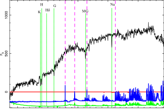
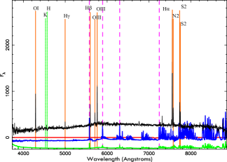
Figure 1: Two examples of reduced spectra are shown. Top panel: An absorption line galaxy in the field with redshift quality 5. Bottom panel: An emission line galaxy in the field with redshift quality of 5. In each plot, the galaxy spectrum (black line), residual spectrum after sky subtraction (green or light grey spectra in the black and white version), sky spectrum (blue / dark grey spectra) and the Telluric absorption spectrum (red or grey horizontal line) are superimposed. The emission (solid orange or medium grey vertical lines) and absorption (dotted green or light grey vertical lines) features at the best fitted redshift are also shown. The most intensive night sky emission lines are demonstrated with dashed vertical magenta (medium grey) lines.

5 Redshift Extraction Results

Following the redshift extraction using RUNZ, we found that 41 objects of our 337 science targets were stars (88%) which is consistent with the uncertainty level of the SuperCOSMOS star/galaxy classification, that Hambly et al. (2001b) estimated to be $\sim$90% accurate down to m_b = 21. A total of 42 measured redshifts from objects with fairly faint blue magnitudes (18.7 $<m_{b}<$ 20.5) were assigned q$\leq$2 thus they were not included in our analysis. Colless et al. (2001) pointed out that the successful redshift determination rate decreases significantly beyond $m_{b}$ = 19 and our detection success rate (87.5%) is in agreement with their finding for the entire 2dF Galaxy Redshift Survey. After the removal of the misclassified stars and non-detected galaxies the remaining 254 targets observed here were classified as galaxies with reliable redshifts. We have supplemented our redshift sample with available redshifts in the literature. We searched the NED up to one degree radius from the core of A3888 for reliable spectroscopic redshifts. We then co-added our spectroscopic redshifts to the published redshifts to build a final redshift sample containing 1027 spectroscopic redshifts.

Table 1 presents the details of the new spectroscopic redshifts obtained by AAOmega and presented in this work. We note that despite the fact that we excluded the objects with available redshifts in the literature in our configuration file, ultimately we still had 15 galaxies in common between our AAOmega observations and the LARCS project. We find that this was because the reported positions in the NED have more than a 3$\arcsec$ separation from the reported positions in SuperCOSMOS and thus, they were missed in the cross matching process. The list of the common objects between our AAOmega observation and the LARCS are given in Table 2.

Table 1: Details of the objects observed with the AAOmega. Columns 1 and 2 give the J2000 coordinates of the object, Columns 3 and 4 give the redshift and its uncertainty, Column 5 is the quality flag, Column 6 is the spectral lines detected, Columns 7 gives the spectral type and finally Column 8 is the blue magnitude from the SuperCOSMOS catalogue. This Table presents the first 10 lines and the full table of 254 galaxies will be available online.

RA	Dec	z	error	Quality	Spectral lines	Spectral type	Blue mag
22 32 02.41	-37 52 50.48	0.19935	0.00016	5	OII,H$\alpha$,N2,S1,S2,H$\beta$	Em	18.96
22 32 08.90	-37 38 53.20	0.16385	0.00016	5	H,K,H$\delta$,G,Na	Abs	19.46
22 32 11.88	-37 43 11.60	0.20863	0.00013	5	OII,H$\alpha$,N2,S1,S2,H$\beta$,OIII	Em	19.35
22 32 15.43	-37 37 23.34	0.03880	0.00010	5	OII,H$\alpha$,N2,S1,S2,H$\beta$,OIII	Em	17.57
22 32 16.22	-37 52 27.08	0.07337	0.00010	5	OII,H$\alpha$,N2,S1,S2,H$\beta$,OIII	Em	18.64
22 32 19.76	-37 41 35.63	0.03838	0.00016	5	OII,H$\alpha$,N2,S1,S2,H$\beta$,OIII	Em	20.07
22 32 20.90	-37 42 53.93	0.38120	0.00011	5	OII,H$\alpha$,N2,S1,S2,H$\beta$,OIII	Em	19.09
22 32 21.10	-37 55 55.02	0.14667	0.00015	5	OII,H$\alpha$,S1,S2,N2	Em	19.22
22 32 21.34	-37 30 30.92	0.20933	0.00013	5	OII,H$\alpha$,N2,S1,S2,H$\beta$,OIII	Em	18.97
22 32 21.54	-37 51 09.72	0.03188	0.00017	5	OII,H$\alpha$,N2,S1,S2,H$\beta$,OIII	Em	19.40

Table 2: List of common observed galaxies. All the common galaxies were also observed in the LARCS project.

RA (J2000), Dec(J2000)	zAAOmega	zerr	zLARCS	zerr
22 32 29.7   -37 37 34	0.13942	0.00025	0.13973	0.00140
22 33 13.3   -37 46 54	0.13993	0.00027	0.13933	0.00260
22 33 19.5   -37 42 12	0.13133	0.00031	0.13182	0.00056
22 33 42.0   -37 45 45	0.15194	0.00022	0.15213	0.00050
22 33 54.4   -37 42 34	0.14702	0.00036	0.14696	0.00011
22 34 16.8   -37 49 13	0.15162	0.00033	0.15140	0.00007
22 34 22.5   -38 03 38	0.12511	0.00058	0.12546	0.00010
22 34 42.3   -37 22 40	0.20857	0.00058	0.20890	0.00110
22 34 45.2   -37 39 51	0.15590	0.00037	0.16223	0.00009
22 34 49.7   -37 29 52	0.14086	0.00016	0.14505	0.00010
22 34 49.9   -37 47 50	0.15250	0.00039	0.15282	0.00020
22 35 27.0   -37 25 42	0.12576	0.00005	0.12570	0.00096
22 35 45.3   -37 21 23	0.14065	0.00042	0.14491	0.00060
22 36 03.9   -37 39 09	0.20138	0.00016	0.20208	0.00120
22 36 19.5   -37 38 30	0.19754	0.00016	0.19740	0.00230

For cases where an object had two redshift measurements, our redshift was chosen if q$\geq$4 otherwise the redshift from the literature was used in our analysis. For all such galaxies, the DSS blue image was visually inspected to ensure that the cross-matching process did not conflate two separate objects and they were indeed true cross-matches. Figure 2 shows the consistency between our extracted redshifts and the redshifts from the literature (for our 15 common redshifts). The plot shows that the majority of our common redshifts are in good agreement with the published redshifts.

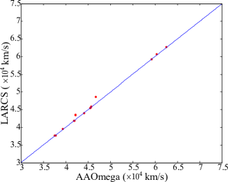
Figure 2: Common objects between the AAOmega observations and the literature, the error bars are not shown due to being smaller than the size of the dots on the plot (the error mean value is about 0.0003 in z or 90 km/s). The solid line is the one-to-one relation.

A colour-coded histogram of the combined redshifts from the final catalogue in a one degree radius around A3888 is shown in Figure 3. The redshift distribution clearly shows the existence of seven distinct populations around A3888. The populations span the redshift range 0.0001–0.4580. The redshift range associated with each population was determined based on conspicuous gaps in the redshift histogram. In Table 3, the redshift range and the number of galaxies in each of identified velocity groups in the combined AAOmega and literature redshift sample are shown.

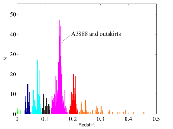
Figure 3: The colour-coded redshift histogram of the combined redshifts (AAOmega + literature) in a one degree radius around the core of A3888. According to this plot, there are seven distinguishable populations up to the redshift of 0.35. See Table 3 for details.

Table 3: Details of the velocity groups and number of galaxies in each redshift slice in a one degree radius around A3888. The largest structure in velocity is clearly A3888 and its outskirts with 469 member galaxies and an extent of $\sim$10 Mpc in radius.

Redshift Range	Ngal
0.0001 – 0.0108	8
0.0284 – 0.0475	80
0.0530 – 0.0875	163
0.0880 – 0.1190	67
0.1200 – 0.1850	469
0.1850 – 0.2220	156
0.2230 – 0.4580	84

6 Spectroscopic Redshift Completeness

Completeness of our redshift sample was determined by calculating the ratio of galaxy number density in the combined redshift catalogue (AAOmega+literature with the upper limit of m_b = 21.32) to the number density of galaxies with available blue magnitudes in the SuperCOSMOS catalogue which is 90% complete up to blue magnitude of 21. There were 937 galaxies out of 1027 galaxies in our redshift sample which had available blue magnitude in the SuperCOSMOS catalogue. The final spectroscopic completeness was scaled by multiplying the ratio of the number of redshifts with available blue magnitude to the total number of available redshifts. Figure 4 shows the cumulative spectroscopic completeness of our final redshift sample as a function of blue magnitude. As it is expected, the spectroscopic completeness decreases whilst the blue magnitude cut increases from top left to bottom right. In some regions the completeness increases, however this unexpected behaviour has been previously seen in other works. For instance, Owers et al. (2011) presented the completeness of the spectroscopic observation of Abell 2744 with the AAOmega and they have observed the same behaviour in some regions. This is suggestive of an anisotropic redshift coverage as a function of magnitude.

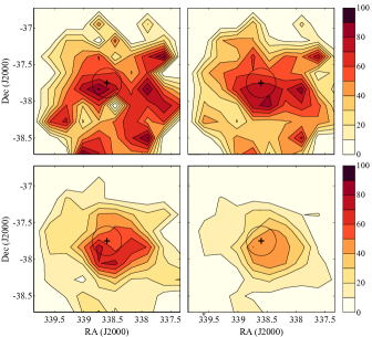
Figure 4: Spectroscopic completeness map of A3888. Top left panel: spectroscopic completeness in $m_{b}\leq$ 18. Top right panel: completeness in $m_{b}\leq$ 19. Bottom left panel: completeness in $m_{b}\leq$ 20. Bottom right panel: completeness in $m_{b}\leq$ 21. Black cross shows the position of A3888 and the black circle shows a region with radius of 2 Mpc around A3888.

Figure 4 also shows that the completeness decreases whilst moving radially outwards which is in agreement with giving a low priority to the outermost regions which are considered as the outskirts of A3888 in our AAOmega configuration procedure. In Figure 5 the left plot shows the cumulative spectroscopic completeness as a function of radius from the core of A3888. According to this plot the completeness is above 30% in all radial bins for all magnitude ranges. The low completeness value in the first radial bin of 500 kpc from the cluster core indicates that the central region of the cluster was extremely over-dense and AAOmega was unable to cover the very dense cluster core due to the physical size of the fibre buttons 3$\arcsec$, $\sim$2.77 kpc at the redshift of cluster) and the minimum required fibre separation of 30^″. The right plot in Figure 5 shows the redshift completeness in different magnitude bins within a 3 Mpc radius from A3888. This plot shows that the spectroscopic completeness is at least 38% within a 3 Mpc radius from the core of A3888 in all magnitude bins whilst the magnitude is brighter than m_b = 20.5.

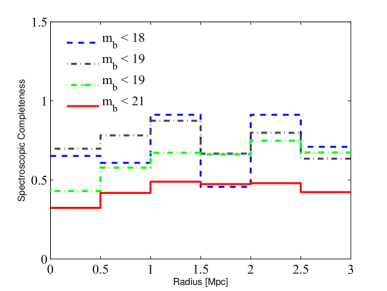
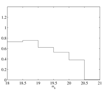
Figure 5: Left panel: cumulative spectroscopic redshift completeness in radial bins of 500 kpc. Right panel: spectroscopic redshift completeness as a function of magnitude within a 3 Mpc radius from the cluster core.

7 Cluster Membership

Decades of optical observations of galaxy clusters have revealed that the majority of galaxy clusters host a single or multiple substructures allowing a broad classification as either dynamic or relaxed systems, respectively. The presence of substructure in a cluster is likely indicative of ongoing dynamical interactions. Substructures may be formed through the infall of individual galaxies or galaxy groups into a relaxed cluster or during the merging of two or more entire galaxy clusters. According to theoretical studies and simulations of galaxy clusters, member galaxies of virialised clusters are expected to exhibit a well-behaved Gaussian velocity distribution (Owers et al., 2009). Therefore, any sign of non-Gaussian behaviour in the velocity distribution can be a signpost of certain conditions such as existence of fore/background interloper galaxies and more importantly, substructure in the cluster (Pinkney et al., 1996; Owers et al., 2009). However, it should be noted that a well established single Gaussian in velocity distribution does not necessarily indicate that the cluster is in dynamical equilibrium (Owers et al., 2009). For instance, the cluster Abell 3667, which has been well studied in the past, is known to be a highly disturbed cluster, however Johnston-Hollitt et al. (2008b) and Owers et al. (2009) pointed out that this cluster has a well described Gaussian velocity distribution as measured along the line of sight, transverse to the known plane of the sky merger axis.

Additionally, interlopers may cause non-Gaussian behaviour in the velocity distribution which can be mistaken as true substructure (Owers et al., 2009). Hence, it is imperative to minimise fore/background galaxy contamination in the cluster field. To achieve this, spatial and LOS peculiar velocity distributions of galaxies are used solely or in a combined manner to determine the cluster members before any further substructure analysis is under taken.

The interloper rejection and cluster member selection for A3888 was performed combining two methods: a Density-Based Spatial Clustering of Applications with Noise (DBSCAN) algorithm (Ester et al., 1996) and the caustic technique (Diaferio & Geller, 1997).

7.1 DBSCAN Clustering Algorithm

The initial cut of the foreground and background galaxies (see Section 5) was carried out by identifying the velocity gaps in the redshift histogram. Further outlier removal was performed by employing the DBSCAN method. This technique has been recently used in different fields of Astrophysics to statistically aggregate data in complex, irregularly sampled datasets, for instance Tramacere & Vecchio (2013) and Carlson et al. (2013) adopted it in analysing the Fermi-LAT gamma ray datasets. More recently Dehghan & Johnston-Hollitt (2014) used this method to detect and allocate members to the galaxy groups and clusters in the Chandra Deep Field-South (CDFS) demonstrating the power of this technique for detecting large-scale structure and its sub-components. We used the DBSCAN function of the open source package fpc (“fixed point clusters”) implemented in the Comprehensive R Archive Network (CRAN). The DBSCAN function in this package follows the procedure introduced by Ester et al. (1996).

The DBSCAN technique requires two user-defined input parameters: the minimum number of points (MinPts) which defines the minimum accepted number of the structure members, and the neighbourhood radius to search for the members associated with each structure (Ester et al., 1996). All of the data points have a classification as core, border or noise. This method is mainly based on calculating the density of individual data points in the sample. The number of all data points within the radius “Eps” is referred to as the density of that particular point. In the calculation of the density, the data point, itself, should be taken into account (Ester et al., 1996). In the case that the number density of a point is greater than MinPts, that point is considered as a core point. A border point is not a core point but it is still within the Eps radius vicinity of a core point and has lower number density value. The points which are not in the Eps radius proximity of the core points are classified as noise. All the steps in the DBSCAN procedure are described below:

1. An arbitrary data point is chosen as a starting point. If the density of that point exceeds the MinPts value, then that point is considered as a core point, otherwise another non-classified data point will be retrieved and the same procedure is repeated. Once all the core points are found, the process finds the border and noise points until all the core and border points are classified. Then, all the noise points will be removed from the sample and will not be further involved in processing.

2. An arbitrarily core point is chosen and is allocated to the first structure. Then, any core point in the Eps-neighbourhood of that core point is also allocated to the first structure. This process recursively searches for other non-allocated core points within the Eps radius around each core point and allocates them all to the first structure. This procedure is repeated till all the border points in the Eps-neighbourhood of allocated core points are also allocated to the first structure. The process is halted when there are no core or border point left to be assigned to the structure.

3. A new core point which is not a member of any pre-detected cluster is retrieved and step 2 is repeated and further clusters are discovered.

4. All the steps are repeated until all the data points are assigned to a cluster.

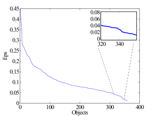
Figure 6: The sorted k-dist plot with k=6. The zoomed inset shows the change in the slope of this k-dist graph. The values which are corresponding to strong changes in the slope are used as the Eps values for the DBSCAN algorithm. The vertical axis has units of degrees and the horizontal axis has no physical unit. The 6-dist sorted plot shows an abrupt change around Eps= 0.027 ($\sim$ 270 kpc at redshift of cluster) and accordingly, the detected structures had proper scales.

The DBSCAN method has some advantages over the widely used Gaussian mixture model clustering algorithm in which velocity groupings are identified by determining a combination of various fitted Gaussians to the dataset (Ashman et al., 1994). The Gaussian mixture clustering approach requires an initial guess of the total number of groupings and the mean of each fitted Gaussian distribution. However, DBSCAN does not need a prior guess of the number of structures. In addition, DBSCAN is not restricted to detect any particular symmetric shape for the groupings. However, the initial estimate of input parameters (MinPts, Eps) can broadly affect the detected structures by DBSCAN. To avoid blind guessing of the input parameters, Ester et al. (1996) suggested to use a so called k-dist plot to choose the Eps value.

The k-dist plot can be constructed following two steps: 1) the distance to the k^th (k = MinPts-1) nearest neighbour for each data point is calculated, 2) the distance values should be sorted in descending manner and plotted. Since the k value is MinPts-1, choosing a k $\leq$ 6 leads to detection of many false groups with a small number of members. The best Eps value is the one where the k-dist plot shows an abrupt change in the slope. The physical meaning is such that all the objects on the right side of the chosen Eps value are considered as core points. Thus, choosing a very small Eps value leads to less detected structures whereas large Eps values tend to merge separate objects. We have examined all the possible Eps values with fixed MinPts=7 in the DBSCAN application and found that Eps= 0.027 ($\sim$ 270 kpc at redshift of A3888) is the value of interest and corresponds to structures with physical scales e.g. galaxy groups. Figure 6 shows the sorted 6-dist plot.

7.2 Caustic Technique

In order to use the information of peculiar velocity of the galaxies in our cluster member selection procedure, the caustic technique was used alongside the DBSCAN application. For this purpose, we used the CAUSTIC APP, an open source application initially developed by Ana Laura Serra (Serra, 2014).

Serra & Diaferio (2013) pointed out that “the caustic technique (Diaferio & Geller, 1997; Diaferio, 1999, 2009; Serra et al., 2011) identifies the escape velocity profile of galaxy clusters from their centre to radii as large as $3R_{200}$”. This radius is considered as the point in the cluster outskirts right before the warm-hot intergalactic medium (WHIM) dominates the region (Reiprich et al., 2013). It is believed that the WHIM is the remaining hot gas from galaxy formation activities in the past (Reiprich et al., 2013).

The caustic method has been extensively employed to estimate the mass profile of galaxy clusters at distances much larger than the virial radius ($\approx R_{200}$) (Regos & Geller, 1989; Diaferio, 1999; Rines & Diaferio, 2006; Serra et al., 2011). However, this method is also a valuable technique to trace the imprints of the gravitational potential well of the galaxy cluster at radii up to few megaparsecs.

Galaxy clusters lie at the knots of filaments of galaxies in the cosmic web. Since gravity is a long-range acting force, galaxies at much larger distances of the order of 10 Mpc will still be affected by the gravity of the cluster (Diaferio & Geller, 1997). During mass accretion in the outskirts of the clusters, galaxies are accelerated by the cluster gravitational potential and consequently fall into the cluster. The aforementioned galaxies ultimately become a gravitationally bound member of the parent cluster. This process creates a characteristic trumpet-shaped escape velocity profile/putative caustic profile for all the galaxies which are interacting with the gravitational potential well of the cluster (Kaiser, 1987; Regos & Geller, 1989; van Haarlem & van de Weygaert, 1993).

The principal assumption in the caustic method is that clusters are spherical and symmetric systems, however, the cluster’s morphology does not affect the caustic profile. The amplitude of the caustics, $A(r)$, is a combination of escape velocity profile and the velocity anisotropy parameter, $\beta(r)$, which is given by:

$$\beta(r)=1-(\langle v_{\theta}^{2}\rangle+\langle v_{\phi}^{2}\rangle)/2\langle v_{r}^{2}\rangle\;$$ (1)

where $v_{\theta},v_{\phi}$ and $v_{r}$ are longitudinal, azimuthal and radial component of the galaxy velocity in the volume $dr^{3}$ at position r (Diaferio & Geller, 1997). The average squared velocity of galaxies in a sphere with radius r is:

$$\langle v^{2}\rangle=\langle v_{LOS}^{2}\rangle g(\beta)\;.$$ (2)

where $v_{LOS}$ is the line of sight component of the galaxy velocity and

$$g(\beta)=\frac{3-2\beta(r)}{1-\beta(r)}\;.$$ (3)

The escape velocity at the radius r is $\langle v_{esc}^{2}(r)\rangle$ = -2$\phi(r)$ where $\phi(r)$ is the gravitational potential. If we assume that the caustic amplitude, $A(r)$, is the LOS component of the escape velocity $A^{2}(r)=\langle v_{esc,LOS}^{2}\rangle$ then we have:

$$-2\phi(r)=A^{2}(r)g(\beta)\equiv\phi_{B}(r)g(\beta)\;.$$ (4)

This equation shows that the caustic amplitude, $A(r)$, is related to the potential well of the cluster .

To estimate $A(r)$, three major steps should be followed (Serra et al., 2011):

1. Construction of a hierarchical tree based on the calculation of projected binding energy for each pair of galaxies, presumed to have identical mass.

2. Determining a threshold to terminate the growth of the hierarchical tree and find the candidate cluster members.

3. Calculating the cluster centre, galaxy number density, caustic profile and determining optimal cluster members.

At first, the projected pair-wise binding energy of all of the galaxies pairs are used to create a hierarchical tree. In the second step, a threshold should be determined to cut the tree.

Diaferio (1999) explained that in the hierarchical tree, there is a main branch that starts from the root and links “nodes” being places where galaxies are hanging. Each group of galaxies hang from nodes that have a velocity dispersion $\sigma_{n}$. The distribution of velocity dispersions of the nodes shows a characteristic feature which is used to determine the cutting threshold. The velocity dispersion $\sigma_{n}$ begins to drop significantly due to less interloper contamination and then the velocity dispersion begins to flatten until it reaches a node associated with internal structures after which it shows a significant drop. Diaferio (1999) mentioned that most of the galaxies hang from node where the “$\sigma$ plateau” begins, are defined as candidate cluster members. In the last step, the cluster centre and the galaxy density is calculated to estimate the LOS caustics. The caustic profile of A3888 is shown in Figure 7. Red (dark grey) dots represent the determined cluster members which reside within the caustics. The other galaxies in grey are not gravitationally bound to A3888.

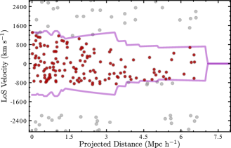
Figure 7: The caustic profile for A3888 (pink solid lines). The red (dark grey) dots show the cluster members defined by the caustic technique. The grey dots are the interloper galaxies which are not gravitationally bound to A3888.

The caustic technique measures the escape velocity profile which can be used as a cluster member allocation tool in the dynamical analysis of the clusters (e.g. Owers et al. 2013, Rines et al. 2013 and Owers et al. 2014 ). The caustic profiles of clusters carry invaluable information about each of the galaxies in the field of cluster. The position of individual galaxies in the caustic profile reflects the time when infall towards the cluster started. Galaxies which are passing the cluster core for the first time have higher caustic amplitudes due to acceleration whereas galaxies which have accreted at the same time that the core of the cluster was forming, tend to be closer to the cluster centre and have lower caustic amplitudes (Haines et al., 2012). The results of the DBSCAN and caustic technique applications are presented in the following sections.

8 Structures in the Main Population of A3888

The colour-coded redshift histogram of the galaxies in a one degree radius around A3888, revealed that members of A3888 fall in the range of 0.12 $<$ z $<$ 0.0185. In Section 7, we explained how the DBSCAN and caustic techniques were used to constrain the interlopers in the galaxy member selection process. These methods allowed us to utilise both redshift and position information to determine the most probable member candidates of A3888.

Firstly, the DBSCAN method was applied to the data in the redshift range 0.12 – 0.0185 and consequently, 77 candidate galaxy members were identified. Further refinement with the caustic method shrunk the number of cluster members to 67 galaxies. In order to verify that the final results were not affected by the order of application, the reverse order (caustic-DBSCAN) was also examined. In the reverse order, the caustic technique was first applied to the data and 146 galaxies were identified as member candidates of the cluster A3888. Then, the DBSCAN method was applied to the caustic method results and 65 galaxies were identified as the final candidate members of A3888. There were 61 galaxies in common in both orders of applications, four extra galaxies were detected in the caustic-DBSCAN order and six further galaxies in DBSCAN-caustic order. Because the caustic-DBSCAN order is more conservative than the reverse order (DBSCAN-caustic) we combined both results and consequently the total number of candidate galaxy members increased to 71.

In addition, the DBSCAN method detected four other galaxy groupings in the redshift range of A3888. The isoline plot of the cluster A3888 and the four detected galaxy grouping are shown in Figure 8. In the following discussion, details of A3888 and other detected structures in redshift slice 0.12 – 0.0185 are given and the five structures are also shown on Figure 8 as numbered groups of coloured points. We have used a method presented by Beers et al. (1990) to estimate the redshift and velocity dispersion of the detected structures. All the reported confidence intervals are calculated based on $\alpha$=0.05 (95$\%$ confidence level). In Table 4 details of the detected groups such as the rest frame velocity dispersion, and observed redshift are given.

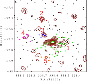
Figure 8: The isoline plot of the groups and cluster A3888 detected by the DBSCAN method. The contours start at 10% and continues in 10% interval to 90%. Dots labelled from 1–5 represent the main cluster A3888 and galaxy groups 2, 3, 4 and 5. See Table 4 for more details.

• Structure 1
  This is the main cluster, A3888 with 71 members. The members are the combined resultant galaxies of caustic-DBSCAN and DBSCAN-caustic applications. The presence of an elongation along a East-West axis might be indicative of sub-clustering in A3888. The estimated average redshift and rest frame velocity dispersion of the cluster were calculated as 0.1535 $\pm$ 0.0009 and 1181 $\pm$ 197 km s^-1, respectively. Details of further substructure tests for the main cluster are given in Section 9.

• Structure 2
  This is a galaxy over-density located in the far North of A3888 and has 7 candidate members at a mean redshift 0.1406. This group was previously reported as a cluster candidate ($\epsilon$) by Pimbblet (2001) based on the redshift measurements of 5 galaxies. However, due to the small number of members, low rest frame velocity dispersion of 338 km s^-1, and lack of an obvious cD galaxy we classify this as a group. The caustic method showed that the galaxy members of this group are not located between the caustics of A3888. Thus, this group is not gravitationally bound to the cluster.

• Structure 3
  This is a galaxy group in the North of cluster A3888 with 5 candidate members. The estimated mean redshift and rest frame velocity dispersion are 0.1411 and 164 km s^-1, respectively. Using the caustic method revealed that the galaxies in this group are not gravitationally bound to the main cluster A3888.

• Structure 4
  This structure with 9 members has two distinct velocity distributions and consequently, the rest frame velocity dispersion at mean redshift of 0.1529 was estimated as 1025 km s^-1 which is considerably higher than the expected velocity dispersion of galaxy groups (400–500 km s^-1). Additionally a visual inspection of the DSS red and blue images failed to suggest a real mass concentration. As a result we believe this is not a real structure, but rather a false grouping.

• Structure 5
  This is a false positive structure featuring a sporadic velocity distribution. There is no evidence of Gaussianity in the velocity distribution. This suggests that this detection is entirely contaminated by projection effects of galaxies which are distributed in a large redshift slice. The estimated mean redshift and rest frame velocity dispersion were 0.1603 and 3232 km s^-1, respectively and again a visual inspection of the DSS images found no evidence of a real group.

Table 4: Details of the detected galaxy groups and the cluster A3888 in the main population. All of the detected structures are in the redshift range of 0.12 – 0.185. The upper and lower limits of the redshift and rest frame velocity dispersion represent the estimated $\alpha$=0.05, 95$\%$ confidence intervals.

Structure ID	Ngal	z	$\sigma_{v,rest}[\mbox{km}$ s-1]	Coord	Comment
1	71	0.1535${}^{+0.0009}_{-0.0009}$	1181${}^{+197}_{-197}$	22 34 31.01  -37 44 06	Cluster A3888
2	7	0.1406${}^{+0.0011}_{-0.0011}$	338${}^{+386}_{-126}$	22 34 52.01  -37 30 21	Galaxy group
3	5	0.1411${}^{+0.0008}_{-0.0008}$	164${}^{+305}_{-66}$	22 34 48.52  -37 39 20	Galaxy group
4	9	0.1529${}^{+0.0037}_{-0.0037}$	1025${}^{+402}_{-402}$	N/A	False galaxy group
5	7	0.1603${}^{+0.0108}_{-0.0111}$	3232${}^{+301}_{-1978}$	N/A	False galaxy group

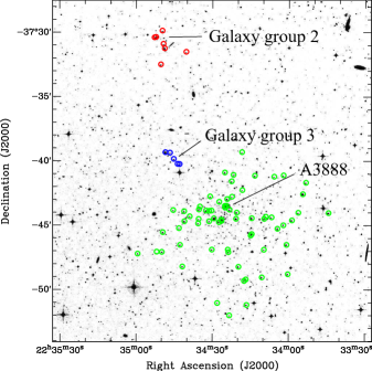
Figure 9: Distribution of member galaxies of cluster A3888 and the two detected groups (Structures 2 $\&$ 3). A3888 and galaxy groups 2 and 3 are demonstrated with green (light grey), red (medium grey) and blue (black) open circles, respectively, on the DSS blue image.

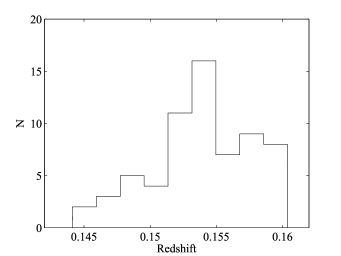
Figure 10: Redshift histogram of the 71 possible members of A3888 shown with a bin width of 540 km s^-1. A departure from Gaussianity is evident around z$\sim$ 0.157.

In Figure 9 the spatial distribution of the member galaxies of A3888 and the detected galaxy groups (structures 2 and 3) are shown. The background image is the DSS blue image.

9 Substructure Test of A3888

In Figure 10 the redshift histogram of the 71 final cluster member candidates is plotted. A departure from Gaussianity is evident around redshift 0.157. In order to verify that this peak in the histogram is statistically significant, we performed a Lee-Fitchett (Lee, 1979; Fitchett, 1988) 3D substructure test using the CALYPSO package (Dehghan & Johnston-Hollitt in prep.). A clipping procedure in the software has automatically rejected four of our 71 candidate member galaxies. According to the substructure test result, A3888 is bimodal. The substructure significance was 99.8$\pm{0.2}\%$ (99.00% confidence level) which is equivalent to a 3.16-sigma detection. However, due to the relatively low redshift sampling of the region, this result is likely subject to change as more redshifts become available in the future. Figure  11 shows the results of the Lee-Fitchett 3D test for A3888. The detected subgroups named G1 and G2 have average redshifts of 0.1505 and 0.1566, respectively. The rest frame velocity dispersion of G1 and G2 were measured as 853$\pm{203}$ and 784$\pm{207}$ km s^-1 at 95% confidence level. Notably the cluster is split into the two subgroups along the same East-West axis as the overall density elongation. Table 5 gives the properties of the two subgroups detected here.

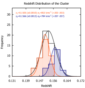
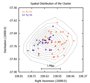
Figure 11: Results of the Lee-Fitchett 3D substructure test of A3888. The cluster is bimodal and the two subgroups are denoted as G1 in red (light grey) and G2 in blue (dark grey). Left plot: histogram of all the members, G1, and G2 are shown with black, red (light grey), and blue (dark grey) lines, respectively. The estimated redshift and rest frame velocity dispersion for G1 and G2 are given in red and blue (light and dark grey), respectively. Right plot: Spatial distribution of the detected groups G1 and G2. The number of candidate members of G1 and G2 are shown in red and blue (light and dark grey), respectively.

Table 5: Details of the detected substructures in A3888.

Groups	Ngal	z	$\sigma_{v,rest}[\mbox{km}$ s-1]
G1	41	0.1505$\pm{0.0010}$	853$\pm{203}$
G2	26	0.1566$\pm{0.0013}$	784$\pm{207}$

We stress that the cumulative redshift coverage is only up to 30% within 1.5 Mpc radius around the cluster where the 71 candidate members reside. Thus, this substructure test is subject to change with improved spectroscopic redshift sampling of the region.

10 Morphological Content of A3888

We have used the spectral atlas of galaxies presented by Kinney et al. (1996) to determine the morphology of the galaxies in our AAOmega sample throughout the redshift determination by RUNZ. All sets of ASCII templates cover the ultraviolet to near infra-red spectral range with the wavelength range of 1235–9935Å. These spectral templates are ideal to identify various galaxy morphologies from elliptical to late type spirals. The full details of the templates for different galaxy morphology are found in Kinney et al. (1996). All of the spectra were visually inspected to confirm the galaxy morphologies determined by RUNZ. We have also used the spectrophotometric atlas of galaxies presented by Kennicutt (1992) to compare our spectra with the reference spectra provided in this atlas. We found that the majority of our observed galaxies across the field of AAOmega were late-type spirals (S_b and S_c). However, these spiral galaxies were mainly field galaxies scattered in various redshift slices. As it is expected, most of the early type galaxies were found in the over-dense regions particularly within a 1 Mpc radius around the core of A3888.

Understanding the evolution of early/late type galaxies in clusters has been one of the major interests in optical astronomy. Recent large spectroscopic surveys (see Section 1), have provided an ideal opportunity to explore the morphological content of galaxy clusters and probe their evolution. For instance, Goto et al. (2003) studied 514 galaxy clusters in the redshift range 0.02 $<$ z $<$ 0.3 from the SDSS. According to their findings, the fraction of blue galaxies at the redshift of A3888 (z = 0.1535) should be around 15$\%$. Later on, Poggianti et al. (2009) investigated the correlation between morphological content of clusters with the cluster’s global properties such as X-ray luminosity and velocity dispersion. They studied the Wide-Field Nearby Galaxy-cluster Survey clusters (WINGS) extensively to examine the effect of cluster properties and environment on the evolution of different galaxy morphology in clusters. WINGS is a multi wavelength photometric and spectroscopic survey of 77 galaxy clusters at 0.04 $<$ z $<$ 0.07 (Fasano et al., 2006). They additionally used 15 high-redshift clusters in former publications to accurately quantify any observed correlation. Poggianti et al. (2009) found that in general, at lower redshifts the morphological content of galaxy clusters are 23:44:33 corresponding to spiral, S0 and elliptical galaxies respectively. Moreover, they found that the spiral fraction of galaxy clusters, inversely correlates with the X-ray luminosity of the parent cluster.

To expand our optical analysis of A3888 and to shed light on the discrepancy associated with the X-ray luminosity, we have investigated the morphological content of A3888 and also verified the location of A3888 with respect to current proposed correlations between the morphological segregation in clusters and the global properties of the parent cluster. Since the majority of redshifts of candidate members of A3888 come from the spectroscopic observations in the LARCS project (Pimbblet et al., 2006), we used the B-R colour reported in the LARCS spectroscopic catalogue to derive the spectral typing of the galaxies in our final redshift sample. This treatment has allowed us to supplement our AAOmega spectral typing information to determine the morphological fraction of the cluster A3888. Pimbblet et al. (2006) reported that the colour of the emission and absorption line galaxies are (B-R)$<$ 1.6 and (B-R)$>$ 2 respectively in their sample, thus galaxies with B-R colour between 1.6 and 2 could be either an absorption or an emission line.

In total, the 71 candidate members of the cluster were comprised of 9 emission line galaxies, 43 absorption line galaxies, 7 galaxies with 1.6 $<$B-R$<$ 2 in the LARCS catalogue and the remaining 12 members had no morphological or spectral typing data available in the literature. Thus of the 52 galaxies with confirmed morphological types, $\sim$ 17% (9/52) are emission line galaxies and $\sim$ 83% (43/52) are absorption line objects. Additionally, for the 19 remaining galaxies (12 without morphological information and 7 with 1.6 $<$B-R$<$ 2) one could assume these could be 100% emission or absorption line to derive the upper and lower limits of morphological content of the cluster. According to these assumptions the estimated emission and absorption fractions are 0.17${}_{0.13}^{0.40}$ and 0.83${}_{0.60}^{0.88}$, respectively. In Figure 12, the two top plots show the correlation between the X-ray luminosity of the parent cluster and the morphological content of the cluster as the fraction of galaxy morphological type in (Poggianti et al., 2009). The location of A3888 is marked with a red filled dot with errors from the limits of the morphological fraction described above. The bottom plots indicate the correlation between the rest frame velocity dispersion and the morphological fraction of the clusters. As can be seen from the plot, the morphological content of A3888 is in agreement with the results derived by Poggianti et al. (2009). Although our redshift coverage is not similar to aforementioned galaxy cluster surveys, our results suggest that the morphological fraction of galaxies in A3888 are in line with the predicted values in large surveys. Additionally we see that the position of A3888 obtained using the X-ray luminosity of Pratt et al. (2009) is consistent with known cluster properties and using either of the previously reported L_x values moves the position of the cluster to a less consistent position. However, we note that the uncertainties on the morphological content make this only a weak argument. Nevertheless it does lend further credence to the X-ray luminosity derived by Pratt et al. (2009).

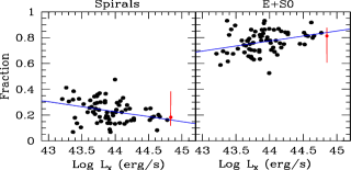
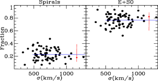
Figure 12: Top panels: the morphological fraction correlation with the X-ray luminosity of the parent cluster is shown with a blue line (Poggianti et al., 2009). Bottom panels: the morphological fraction correlation with the cluster’s rest frame velocity dispersion is shown with a blue line (Poggianti et al., 2009). In all the plots, the location of A3888 is annotated with the filled red dot and a vertical line to denote the uncertainty. The images are adapted from Poggianti et al. (2009) with permission.

11 Foreground and Background Structures

According to the colour-coded histogram (see Figure 3), there are other fore/background populations of galaxies in a one degree radius around A3888. The DBSCAN method was applied to all of the separate populations distributed in the redshift histogram. According to the DBSCAN results, galaxy populations in the light-blue (0.053 $\leq$ z $\leq$ 0.0875) and red (0.185 $\leq$ z $\leq$ 0.222) regions in the colour-coded histogram (Figure 3) host galaxy clusters and galaxy groups.

Examination of the DSS blue image revealed existence of three cD galaxies in the field with conspicuous mass concentrations around them. Interestingly, the application of the DBSCAN to galaxies in the redshift range 0.053 $\leq$ z $\leq$ 0.0875 (the light blue grouping on Figure 3) confirmed the existence of three galaxy clusters around the aforementioned cD galaxies. Thus, the DBSCAN results were consistent with the visual inspection of the DSS blue image and hereafter these three clusters are denoted as Structures 6,7 and 8. Examination of the redshifts between 0.185 and 0.222 (red population on Figure 3) showed the presence of an additional galaxy group, denoted here as Structure 9.

Table 6 gives the summary of the DBSCAN results on these over-densities and further narrows the ranges over which the structures occur. We also list an IAU name for each new cluster detected. On account of poor redshift coverage, determining all of the members of the detected clusters and galaxy groups is not feasible and all the analysis is based on the available limited measured redshifts.

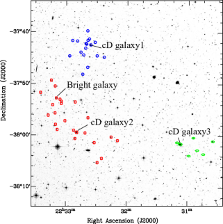
Figure 13: The spatial distribution of galaxies in the detected structures. The cD galaxies of detected galaxy clusters are annotated on the plot. Structure 6 (SJD J2232.4-3742) is shown with blue circles with labelled cD galaxy 1, Structure 7 (SJD J2232.5-3759) is given by red squares with labelled cD galaxy 2 and Structure 8 (SJD J2231.1-3801) is shown with green ellipses with labelled cD galaxy 3. The DSS blue is the background image.

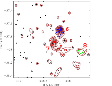
Figure 14: The isoline plot of the galaxies in redshift slice of 0.0717–0.0856. The contour starts from 10% and continues with 10% interval to 90%.

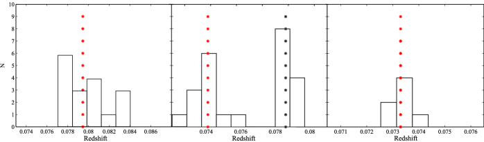
Figure 15: Redshift histogram of the clusters found in the redshift range 0.0717–0.0856. The red (grey) vertical dotted lines represent the redshift of the cD galaxy in each cluster. The black dotted line represents the redshift of the BCG. The redshift histograms of Structures 6 (SJD J2232.4-3742), 7 (SJD J2232.5-3759) and 8 (SJD J2231.1-3801) are shown from left to right, respectively.

Table 6: Details of fore/back ground structures detected by the DBSCAN method in the field of A3888. The upper and lower limits of the redshift and velocity dispersion represent the estimated $\alpha$=0.05, 95$\%$ confidence intervals.

Structure ID	IAU Name	zcD	Ngal	z	$\sigma_{v,rest}$ [km s-1]	cD coord
6	SJD J2232.4-3742	0.0795	17	0.0792${}^{+0.0013}_{-0.0013}$	730${}^{+363}_{-363}$	22 32 35 -37 42 28.93
7	SJD J2232.5-3759	0.0741	24	0.0765${}^{+0.0022}_{-0.0022}$	727${}^{+592}_{-592}$	22 32 49 -37 59 24.91
8	SJD J2231.1-3801	0.0733	7	0.0732${}^{+0.0005}_{-0.0005}$	128${}_{-19}^{+209}$	22 31 07 -38 01 35.95
9	SJD J2234.2-3719	$\ldots$	6	0.2006${}^{+0.0020}_{-0.0020}$	420${}^{+541}_{-175}$	22 34 16 -37 19 25.01a

• The coordinate of the brightest galaxy.

As before, we used the method of Beers et al. (1990) for the calculations of velocity dispersions and redshifts of the detected structures. All of the confidence intervals were estimated based on 95$\%$ confidence level ($\alpha$=0.05).

• Structure 6 – SJD J2232.4-3742
  This structure is a galaxy cluster which has 17 candidate members. The cD galaxy has a redshift of 0.0795 and is denoted as cD galaxy 1 on Figure 13. All of the candidate members of this cluster are annotated with blue open circles on the DSS blue image in Figure 13. The estimated average redshift and rest frame velocity dispersion of the cluster are 0.0792 and 730 km s^-1, respectively. The contour plot of this structure is shown in Figure 14 (blue dots with label 6). In the left plot in Figure 15 the redshift histogram of this cluster is shown. The details of this structure is given in Table 6 and the member galaxies are repoted in Table 7. We stress that the velocity dispersion might have been underestimated because of poor sampling in this region.

• Structure 7 – SJD J2232.5-3759
  This structure is a galaxy cluster which has 24 candidate members with a cD galaxy with redshift of 0.0741 which is denoted as cD galaxy 2 on Figure 13. The candidate members with red open squares are shown in Figure 13. The average redshift and the rest frame velocity dispersion of this cluster is 0.0765 and 727 km s^-1, respectively. The contour plot of this structure is shown in Figure 14 (red dots with label 7). The middle plot in Figure 15 shows the redshift histogram of this cluster with two well-separated redshift distribution which might explain the large estimated intervals of the velocity dispersion. The left peak in the histogram is consistent with the redshift of the cD galaxy. Additionally, the right peak in the histogram is in line with the redshift of a bright galaxy (z = 0.0786) which is probably the Brightest Cluster Galaxy (BCG) of an interacting cluster and is also denoted as “Bright galaxy” in Figure 13. The projected distance (estimated at the mean redshift of both galaxies) between these two galaxies is 695 kpc. Figure 16 shows the two populations of galaxies with different velocity distributions according to the histogram shown in middle plot in Figure 15. The redshift distribution might be a signpost of an dynamical interaction between a galaxy cluster and a group or another cluster of galaxies. Table 6 gives details of this structure and the member galaxies are repoted in Table 7. Further analysis requires greater redshift sampling of this region.

• Structure 8 – SJD J2231.1-3801
  This is a galaxy cluster with 7 members which has an average redshift of 0.0732 and hosts a cD galaxy with z= 0.0733 which is denoted as cD galaxy 3 in Figure 13. The candidate members are annotated with green open ellipses in Figure 13. The contour plot of this structure is shown in Figure 14 (green dots with label 8). The right plot in Figure 15 shows the redshift histogram of this cluster. The redshift of the cD galaxy is in line with the peak of the histogram. On account of insufficient redshift coverage the rest frame velocity dispersion (128 km s^-1) will be highly underestimated, but is sufficient for a group. Table 6 gives details of this structure and the member galaxies are repoted in Table 7.

• Structure 9 – SJD J2234.2-3719
  There is another galaxy group found in the redshift slice of 0.1867–0.2162. This is a very small group of merely six galaxies. The average redshift and rest frame velocity dispersion of this group are 0.2006 and 420 km s^-1, respectively. The estimated velocity dispersion has a large confidence interval which is more likely to be a result of poor sampling. Figure 17 shows the isoline plot of Structure 9 (blue dots with label 9) which is superimposed on the scatter plot. Details of this structure and its member galaxies are given in Table 6.

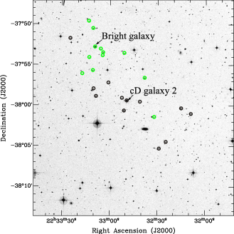
Figure 16: Redshift distribution of Structure 7 (SJD J2232.5-3759) based on the velocity gap in the redshift histogram (see the middle plot in Figure 15). The black circles represent the galaxy population of the left side of the histogram in the redshift range of 0.073–0.077 and the light green circles demonstrate the galaxies in the right side of the histogram in the redshift range of 0.077–0.080. The DSS blue is the background image.

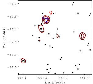
Figure 17: Contour plot of Structure 9 (SJD J2234.2-3719). The contour levels are 50%, 70% and 90%.

We note that there are four other galaxy clusters reported in the literature in a one degree radius around A3888 (ABELL 3896 NED01 & ABELL 3896 NED02, Batuski et al. 1999, ABELL S1045, Dalton et al. 1994 and ABELL S1051, Collins et al. 1995). There are also three galaxy groups reported in this region (LCLG -39 198 & LCLG -39 199 Tucker et al. 2000 and USGC S275, Mahdavi et al. 2000) however, none of there were re-detected in this work. Given the large distance of these clusters to A3888 and our poor redshift coverage in the far field of A3888, it was highly unlikely for us to find these clusters.

Based on an search for galaxy over-densities in the optical images associated with the LARCs project using the local galaxy density parameter, $\Sigma$, Pimbblet (2001) identified six over-densities of which he put forward five candidate clusters in the field around A3888. Examination of colour magnitude diagrams suggested that several of these were likely clusters, however there was a lack of spectroscopic information for the majority of putative cluster members. Of note are three objects listed in Pimbblet (2001) which he denoted $\alpha$, $\beta$ and $\epsilon$ which correspond to Structures 7, 6 and 2, respectively. Comparison of the redshifts present by Pimbblet (2001) and those given here shows that for Structure 7 – SJD J2232.5-3759 the single redshift presented by Pimbblet (2001) is one of the 24 cluster members confirmed here and for Structure 6 – SJD J2232.4-3742 four of the five redshifts listed by Pimbblet (2001) are part of the 17 members listed here and in both cases the use of the local density parameter identifies the same cD galaxy as found here. In the case of Structure 2, five of the seven members were listed previously though we classify this as a group, not a cluster (see Section 8). The three remaining putative over-densities listed in Pimbblet (2001) have not been detected in this work.

12 Discussion and Conclusion

We have presented the results of new optical observations of the cluster A3888 taken with the AAOmega spectrograph. We present 254 new redshifts in the region of A3888. Combining these with available redshifts in the literature we find that main cluster, A3888, has 71 member galaxies, a redshift of 0.1535$\pm$0.0009 and a rest frame velocity dispersion of 1181$\pm$197 km/s. The cluster is elongated along an East-West axis and a 3D Lee-Fitchett substructure test of the cluster indicates that A3888 is a bimodal cluster along that same axis.

The contradictory evidence about the dynamics of A3888 from X-ray data explained earlier underlines that the dynamical status of this cluster was previously not clear. However, the combination of pieces of evidence from the optical analysis such as the presence of multiple BCGs, the elongated optical galaxy distribution, and our substructure test which showed that A3888 is bimodal strongly suggests that this cluster has had dynamical interactions and is highly likely to be a young cluster in an active merging state. This is consistent with the latest X-ray morphology reported by Weißmann et al. (2013) which confirmed that A3888 has local X-ray substructures and a large BCG/X-ray peak separation.

Further spectroscopic analysis of this cluster would be useful to further probe its dynamics, however, on account of the very small angular separation of the galaxies in the core of the cluster, single slit spectroscopy or more usefully observations with an integral field unit are required to increase the spectroscopic coverage in the cluster core. This would allow a more detailed probe of the cluster core and better statistics on the merging populations.

In addition to the work on A3888 we also presented six galaxy over-densities within a one degree radius of the clusters, including three new spectroscopically detected galaxy clusters. Again, further observations of these structures, particularly the clusters, would be beneficial.

Appendix A Member Galaxies of the Newly Detected Galaxy Clusters

Table 7: Details of the galaxies of detected galaxy clusters (Structures 6, 7, 8).

R.A	Dec	z
Structure 6 – SJD J2232.4-3742
22 32 22.70	-37 44 54.00	0.07743
22 32 29.68	-37 44 38.11	0.08022
22 32 31.70	-37 42 01.00	0.07998
22 32 35.90	-37 42 31.00	0.07945
22 32 37.40	-37 41 23.00	0.07795
22 32 38.75	-37 41 38.18	0.07834
22 32 38.89	-37 46 52.21	0.08007
22 32 39.03	-37 39 48.06	0.07909
22 32 40.12	-37 42 22.18	0.07814
22 32 40.60	-37 42 16.00	0.07790
22 32 41.00	-37 43 10.00	0.08454
22 32 42.90	-37 44 29.00	0.07972
22 32 43.70	-37 48 13.00	0.08439
22 32 45.60	-37 43 56.00	0.08297
22 32 49.00	-37 41 47.00	0.08095
22 32 53.80	-37 41 41.00	0.08433
22 32 56.60	-37 44 40.00	0.07692
Structure 7 – SJD J2232.5-3759
22 32 09.10	-38 01 01.00	0.07401
22 33 10.20	-37 57 56.00	0.07366
22 32 15.20	-38 00 20.00	0.07345
22 32 24.70	-38 04 29.00	0.07361
22 32 29.00	-38 05 19.00	0.07449
22 32 32.10	-38 01 25.00	0.07926
22 32 38.20	-37 56 36.00	0.07813
22 32 41.10	-37 59 33.00	0.07614
22 32 49.40	-37 59 24.00	0.07413
22 32 51.00	-37 53 33.00	0.07906
22 32 51.10	-38 00 39.00	0.07411
22 33 00.91	-37 57 12.20	0.07203
22 33 04.30	-37 53 29.00	0.07828
22 33 04.61	-37 53 50.89	0.07865
22 33 05.80	-37 53 02.00	0.07881
22 33 08.70	-37 58 52.00	0.07410
22 33 09.40	-37 52 47.00	0.07859
22 33 10.20	-37 57 56.00	0.07366
22 33 10.60	-37 50 30.00	0.07834
22 33 10.70	-37 55 41.00	0.07847
22 33 13.00	-37 54 05.00	0.07891
22 33 13.26	-37 49 36.16	0.07845
22 33 17.34	-37 56 05.10	0.07970
22 33 24.90	-37 51 44.00	0.07473
Structure 8 – SJD J2231.1-3801
22 30 34.70	-38 01 00.00	0.07436
22 30 44.00	-38 03 31.00	0.07253
22 30 50.10	-38 02 47.00	0.07351
22 30 53.90	-38 00 20.00	0.07312
22 30 58.20	-38 03 51.00	0.07327
22 31 07.20	-38 01 36.00	0.07329
22 31 10.10	-38 01 16.00	0.07325

References

- Abazajian et al. (2009) Abazajian K. N., et al., 2009, ApJS, 182, 543
- Ashman et al. (1994) Ashman K. M., Bird C. M., Zepf S. E., 1994, AJ, 108, 2348
- Batuski & Burns (1985) Batuski D. J., Burns J. O., 1985, ApJ, 299, 5
- Batuski et al. (1999) Batuski D. J., Miller C. J., Slinglend K. A., Balkowski C., Maurogordato S., Cayatte V., Felenbok P., Olowin R., 1999, ApJ, 520, 491
- Beers et al. (1990) Beers T. C., Flynn K., Gebhardt K., 1990, Astronomical Journal, 100, 32
- Bertschinger & Gelb (1991) Bertschinger E., Gelb J. M., 1991, Computers in Physics, 5, 164
- Böhringer & Werner (2010) Böhringer H., Werner N., 2010, A&ARv, 18, 127
- Böhringer et al. (2007) Böhringer H., et al., 2007, A&A, 469, 363
- Böhringer et al. (2010) Böhringer H., et al., 2010, A&A, 514, A32
- Borgani et al. (2002) Borgani S., Governato F., Wadsley J., Menci N., Tozzi P., Quinn T., Stadel J., Lake G., 2002, MNRAS, 336, 409
- Briel & Henry (1994) Briel U. G., Henry J. P., 1994, Nature, 372, 439
- Brunetti & Lazarian (2007) Brunetti G., Lazarian A., 2007, MNRAS, 378, 245
- Brunetti & Lazarian (2011) Brunetti G., Lazarian A., 2011, MNRAS, 410, 127
- Caldwell & Rose (1997) Caldwell N., Rose J. A., 1997, AJ, 113, 492
- Carlson et al. (2013) Carlson E., Linden T., Profumo S., Weniger C., 2013, Phys. Rev. D, 88, 043006
- Chon et al. (2012) Chon G., Böhringer H., Smith G. P., 2012, A&A, 548, A59
- Colless (1999) Colless M., 1999, in Efstathiou G., et al. eds, Large-Scale Structure in the Universe. p. 105
- Colless & Dunn (1996) Colless M., Dunn A. M., 1996, ApJ, 458, 435
- Colless et al. (2001) Colless M., et al., 2001, MNRAS, 328, 1039
- Collins et al. (1995) Collins C. A., Guzzo L., Nichol R. C., Lumsden S. L., 1995, MNRAS, 274, 1071
- Dalton et al. (1994) Dalton G. B., Efstathiou G., Maddox S. J., Sutherland W. J., 1994, MNRAS, 269, 151
- Dehghan & Johnston-Hollitt (2014) Dehghan S., Johnston-Hollitt M., 2014, AJ, 147, 52
- Diaferio (1999) Diaferio A., 1999, MNRAS, 309, 610
- Diaferio (2009) Diaferio A., 2009, preprint, (arXiv:0901.0868)
- Diaferio & Geller (1997) Diaferio A., Geller M. J., 1997, ApJ, 481, 633
- Dressler & Shectman (1988) Dressler A., Shectman S. A., 1988, AJ, 95, 985
- Ebeling et al. (1996) Ebeling H., Voges W., Bohringer H., Edge A. C., Huchra J. P., Briel U. G., 1996, MNRAS, 281, 799
- Ester et al. (1996) Ester M., Kriegal H. P., Sander J., 1996, Proc. 2nd Int. Conf. on Knowledge Discovery and Data Mining (KDD’96). AAAI Press, Menlo Park, CA, pp 226–231
- Fasano et al. (2006) Fasano G., et al., 2006, A&A, 445, 805
- Fassbender et al. (2011) Fassbender R., et al., 2011, A&A, 527, A78
- Fitchett (1988) Fitchett M., 1988, MNRAS, 230, 161
- Geller & Beers (1982) Geller M. J., Beers T. C., 1982, PASP, 94, 421
- Geller & Huchra (1989) Geller M. J., Huchra J. P., 1989, Science, 246, 897
- Girardi et al. (2016) Girardi M., et al., 2016, MNRAS, 456, 2829
- Goto et al. (2003) Goto T., et al., 2003, PASJ, 55, 739
- Gott et al. (2005) Gott III J. R., Jurić M., Schlegel D., Hoyle F., Vogeley M., Tegmark M., Bahcall N., Brinkmann J., 2005, ApJ, 624, 463
- Haarsma et al. (2009) Haarsma D. B., Leisman L., Bruch S., Donahue M., 2009, in American Astronomical Society Meeting Abstracts 213. p. 448.23
- Haarsma et al. (2010) Haarsma D. B., et al., 2010, ApJ, 713, 1037
- Haines et al. (2012) Haines C. P., et al., 2012, ApJ, 754, 97
- Hambly et al. (2001a) Hambly N. C., et al., 2001a, MNRAS, 326, 1279
- Hambly et al. (2001b) Hambly N. C., Irwin M. J., MacGillivray H. T., 2001b, MNRAS, 326, 1295
- Hess et al. (2015) Hess K. M., Jarrett T. H., Carignan C., Passmoor S. S., Goedhart S., 2015, MNRAS, 452, 1617
- Hoyle & Vogeley (2004) Hoyle F., Vogeley M. S., 2004, ApJ, 607, 751
- Johnston-Hollitt et al. (2008a) Johnston-Hollitt M., Sato M., Gill J. A., Fleenor M. C., Brick A.-M., 2008a, MNRAS, 390, 289
- Johnston-Hollitt et al. (2008b) Johnston-Hollitt M., Hunstead R. W., Corbett E., 2008b, A&A, 479, 1
- Jones & Forman (1984) Jones C., Forman W., 1984, ApJ, 276, 38
- Jones et al. (2009) Jones D. H., et al., 2009, MNRAS, 399, 683
- Kaiser (1987) Kaiser N., 1987, MNRAS, 227, 1
- Kennicutt (1992) Kennicutt Jr. R. C., 1992, ApJS, 79, 255
- Kinney et al. (1996) Kinney A. L., Calzetti D., Bohlin R. C., McQuade K., Storchi-Bergmann T., Schmitt H. R., 1996, ApJ, 467, 38
- Klypin et al. (2011) Klypin A. A., Trujillo-Gomez S., Primack J., 2011, ApJ, 740, 102
- Kravtsov & Borgani (2012) Kravtsov A. V., Borgani S., 2012, ARA&A, 50, 353
- Krick et al. (2006) Krick J. E., Bernstein R. A., Pimbblet K. A., 2006, AJ, 131, 168
- Lee (1979) Lee k. L., 1979, J.Am.Stat.Assoc, 74, 708–714
- Lidman et al. (2013) Lidman C., et al., 2013, MNRAS, 433, 825
- Mahdavi et al. (2000) Mahdavi A., Böhringer H., Geller M. J., Ramella M., 2000, ApJ, 534, 114
- Mann & Ebeling (2012) Mann A. W., Ebeling H., 2012, MNRAS, 420, 2120
- Markevitch et al. (2002) Markevitch M., Gonzalez A. H., David L., Vikhlinin A., Murray S., Forman W., Jones C., Tucker W., 2002, ApJ, 567, L27
- Markevitch et al. (2005) Markevitch M., Govoni F., Brunetti G., Jerius D., 2005, ApJ, 627, 733
- Oogi et al. (2016) Oogi T., Habe A., Ishiyama T., 2016, MNRAS, 456, 300
- Overzier et al. (2013) Overzier R., Lemson G., Angulo R. E., Bertin E., Blaizot J., Henriques B. M. B., Marleau G.-D., White S. D. M., 2013, MNRAS, 428, 778
- Owers et al. (2009) Owers M. S., Couch W. J., Nulsen P. E. J., 2009, ApJ, 693, 901
- Owers et al. (2011) Owers M. S., Randall S. W., Nulsen P. E. J., Couch W. J., David L. P., Kempner J. C., 2011, ApJ, 728, 27
- Owers et al. (2013) Owers M. S., et al., 2013, ApJ, 772, 104
- Owers et al. (2014) Owers M. S., et al., 2014, ApJ, 780, 163
- Peebles (1980) Peebles P. J. E., 1980, The large-scale structure of the universe
- Pimbblet (2001) Pimbblet K. A., 2001, PhD thesis, University of Durham
- Pimbblet et al. (2006) Pimbblet K. A., Smail I., Edge A. C., O’Hely E., Couch W. J., Zabludoff A. I., 2006, MNRAS, 366, 645
- Pimbblet et al. (2013) Pimbblet K. A., Shabala S. S., Haines C. P., Fraser-McKelvie A., Floyd D. J. E., 2013, MNRAS, 429, 1827
- Pinkney et al. (1996) Pinkney J., Roettiger K., Burns J. O., Bird C. M., 1996, ApJS, 104, 1
- Plagge et al. (2010) Plagge T., et al., 2010, ApJ, 716, 1118
- Planck Collaboration et al. (2011) Planck Collaboration et al., 2011, A&A, 536, A8
- Planck Collaboration et al. (2014) Planck Collaboration et al., 2014, A&A, 571, A16
- Poggianti et al. (2009) Poggianti B. M., et al., 2009, ApJ, 697, L137
- Porter & Raychaudhury (2005) Porter S. C., Raychaudhury S., 2005, MNRAS, 364, 1387
- Pratley et al. (2013) Pratley L., Johnston-Hollitt M., Dehghan S., Sun M., 2013, MNRAS, 432, 243
- Pratt et al. (2009) Pratt G. W., Croston J. H., Arnaud M., Böhringer H., 2009, A&A, 498, 361
- Pratt et al. (2010) Pratt G. W., et al., 2010, A&A, 511, A85
- Press & Schechter (1974) Press W. H., Schechter P., 1974, ApJ, 187, 425
- Randall et al. (2002) Randall S. W., Sarazin C. L., Ricker P. M., 2002, ApJ, 577, 579
- Regos & Geller (1989) Regos E., Geller M. J., 1989, AJ, 98, 755
- Reiprich & Böhringer (2002) Reiprich T. H., Böhringer H., 2002, ApJ, 567, 716
- Reiprich et al. (2013) Reiprich T. H., Basu K., Ettori S., Israel H., Lovisari L., Molendi S., Pointecouteau E., Roncarelli M., 2013, Space Sci. Rev., 177, 195
- Ribeiro et al. (2013) Ribeiro A. L. B., Lopes P. A. A., Rembold S. B., 2013, A&A, 556, A74
- Rines & Diaferio (2006) Rines K., Diaferio A., 2006, AJ, 132, 1275
- Rines et al. (2013) Rines K., Geller M. J., Diaferio A., Kurtz M. J., 2013, ApJ, 767, 15
- Roettiger et al. (1997) Roettiger K., Loken C., Burns J. O., 1997, ApJS, 109, 307
- Roettiger et al. (1998) Roettiger K., Stone J. M., Mushotzky R. F., 1998, ApJ, 493, 62
- Rose et al. (2002) Rose J. A., Gaba A. E., Christiansen W. A., Davis D. S., Caldwell N., Hunstead R. W., Johnston-Hollitt M., 2002, AJ, 123, 1216
- Sarazin (1986) Sarazin C. L., 1986, Reviews of Modern Physics, 58, 1
- Serra (2014) Serra A. L., 2014, CausticApp, http://personalpages.to.infn.it/~serra/causticapp.html
- Serra & Diaferio (2013) Serra A. L., Diaferio A., 2013, ApJ, 768, 116
- Serra et al. (2011) Serra A. L., Diaferio A., Murante G., Borgani S., 2011, MNRAS, 412, 800
- Sharp et al. (2006) Sharp R., et al., 2006, in Society of Photo-Optical Instrumentation Engineers (SPIE) Conference Series. p. 62690G (arXiv:astro-ph/0606137), doi:10.1117/12.671022
- Springel et al. (2001) Springel V., Yoshida N., White S. D. M., 2001, New Astron., 6, 79
- Springel et al. (2005) Springel V., et al., 2005, Nature, 435, 629
- Springel et al. (2006) Springel V., Frenk C. S., White S. D. M., 2006, Nature, 440, 1137
- Subramanian et al. (2006) Subramanian K., Shukurov A., Haugen N. E. L., 2006, MNRAS, 366, 1437
- Sutter et al. (2012) Sutter P. M., Lavaux G., Wandelt B. D., Weinberg D. H., 2012, ApJ, 761, 44
- Sutter et al. (2014) Sutter P. M., Lavaux G., Wandelt B. D., Weinberg D. H., Warren M. S., Pisani A., 2014, MNRAS, 442, 3127
- Tempel et al. (2014) Tempel E., Stoica R. S., Martínez V. J., Liivamägi L. J., Castellan G., Saar E., 2014, MNRAS, 438, 3465
- Tonry & Davis (1979) Tonry J., Davis M., 1979, AJ, 84, 1511
- Tramacere & Vecchio (2013) Tramacere A., Vecchio C., 2013, A&A, 549, A138
- Tucker et al. (2000) Tucker D. L., et al., 2000, ApJS, 130, 237
- Weißmann et al. (2013) Weißmann A., Böhringer H., Šuhada R., Ameglio S., 2013, A&A, 549, A19
- Wesson & Lermann (1977) Wesson P. S., Lermann A., 1977, Ap&SS, 46, 327
- den Hartog & Katgert (1996) den Hartog R., Katgert P., 1996, MNRAS, 279, 349
- van Haarlem & van de Weygaert (1993) van Haarlem M., van de Weygaert R., 1993, ApJ, 418, 544
- van de Weygaert & Platen (2011) van de Weygaert R., Platen E., 2011, International Journal of Modern Physics Conference Series, 1, 41