​​​ LAL 16-009

On the potential of multivariate techniques for the determination of multidimensional efficiencies.

B. Viaud^a

^a LAL, Univ. Paris-Sud, CNRS/IN2P3, Université Paris-Saclay, 91400 Orsay, France

Differential measurements of particle collisions or decays can provide stringent constraints on physics beyond the Standard Model of particle physics. In particular, the distributions of the kinematical and angular variables that characterise heavy meson multibody decays are non trivial and can sign the underlying interaction physics. In the era of high luminosity opened by the advent of the Large Hadron Collider and of Flavor Factories, differential measurements are less and less dominated by statistical precision and require a precise determination of efficiencies that depend simultaneously on several variables and do not factorise in these variables. This document is a reflection on the potential of multivariate techniques for the determination of such multidimensional efficiencies. We carried out two case studies that show that multilayer perceptron neural networks can determine and correct for the distortions introduced by reconstruction and selection criteria in the multidimensional phase space of the decays ${{B}^{0}}\!\rightarrow{{K}^{*0}}(\rightarrow{{K}^{+}}{{\pi}^{-}}){\mu^{+}}{\mu^{-}}$ and ${{D}^{0}}\!\rightarrow{{K}^{-}}{{\pi}^{+}}{{\pi}^{+}}{{\pi}^{-}}$, at the price of a minimal analysis effort. We conclude that this method can already be used for measurements which statistical precision does not yet reach the percent level and that with more sophisticated machine learning methods, the aforementioned potential is very promising.

 

1 Introduction

With the advent of the LHC and, a few years before, of Flavor Factories, High Energy Physics (HEP) entered an era of high statistical precision. More and more differential measurements of particle collisions or decays are now possible. For instance, stringent constraints can be imposed on the models predicting the dynamics of the decay ${{B}^{0}}\!\rightarrow{{K}^{*0}}(\rightarrow{{K}^{+}}{{\pi}^{-}}){\mu^{+}}{\mu^{-}}$ by measuring the distribution of this decay in the four-dimensional space defined by $q^{2}$, cos$\theta_{l}$, cos$\theta_{K}$ and $\phi$, a set of independent variables that provide a full description of the decay dynamics and that are defined in Sect. 2.1. Deviations from the Standard Model (SM) predictions in specific regions of the phase space can be detected this way and sign the action of a physics beyond the SM. Loop-mediated rare decays like ${{B}^{0}}\!\rightarrow{{K}^{*0}}(\rightarrow{{K}^{+}}{{\pi}^{-}}){\mu^{+}}{\mu^{-}}$ are particularly sensitive to this New Physics. Many models in which particles do not couple to weak interaction via only their left chiral component predict angular distributions that differ from the SM ones. More detail can be found, for instance, in Ref. [1].

In analyses of the kind introduced above, one has to account for the distortion of the phase space caused by reconstruction and selection criteria. In the example above, this is the distortion of the ($q^{2}$, cos$\theta_{l}$, cos$\theta_{K}$, $\phi$) distribution. The most straightforward method would be to use a sample of simulated ${{B}^{0}}\!\rightarrow{{K}^{*0}}(\rightarrow{{K}^{+}}{{\pi}^{-}}){\mu^{+}}{\mu^{-}}$ phase-space decays. A four-dimensional binning could be defined, and the efficiency in each bin determined by the ratio between the yield of reconstructed and selected events and the yield of generated events. If this determination is made in terms of all the kinematic variables describing the decay and if the granularity of the binning is fine enough, the result does not depend on the distributions assumed by the simulation for these variables. This assumption often relies on decay models poorly predicted by theory. However, this method would necessit to generate a huge sample. Even with only 10 bins per dimension, 10000 four-dimensional bins have to be defined. It takes typically millions of generated events to determine the efficiency bins with less than a 5% uncertainty. Instead, sophisticated methods are available to account for efficiencies that depend simultaneously on several variables and that do not factorise in these variables (see Sect. 2.1).

We propose in this document to explore the potential of another approach, suggested by rapid progresses in machine learning and multivariate analysis observed in the last decade. Techniques such as Neural Networks (NN) [2] or Boosted Decision Trees (BDT) [3], among others, can now detect with high sensitivity differences between two samples of events characterised by a large number of variables. They are routinely used nowdays in particle physics measurements to tell signal from background events. Said otherwise, these techniques are performant at comparing $n$-dimensional distributions to detect even subtle differences between signal and background samples (that traditional “by eye” studies would miss) and discrimate between event types via the NN or BDT score, a single variable incorporating all the information found in $n$ dimensions. They should naturally be sensitive also to distortions introduced in the phase space of particle collisions or decays by reconstruction and selection criteria.

We do not take for granted that multivariate techniques reach the same level of precision as methods such as the principal moment analysis described in [1], nor that such a result can be obtained without a certain expertise in MVA techniques or without a time-consumming optimisation of the parameters that rule the technique’s behavior and performance. However, the rythm at which MVA techniques have been progressing recently, their growing availability to basic users in the form of user-friendly packages, and the increasing typical expertise of high energy physicists suggest MVAs might soon become very valuable tools, and easy to use, for multidimensional efficiency determination. It is therefore interesting to start exploring the potential of this approach.

This document only starts this exploration, with the ambition to answer the following question: what can be achieved if multivariate techniques are used in a very simple manner, i.e. without devoting more than a few hours to their optimisation — therefore using generic settings, like the default ones found in packages like [4]? In the case of analyses which do not require the same precision as the analysis of ${{B}^{0}}\!\rightarrow{{K}^{*0}}(\rightarrow{{K}^{+}}{{\pi}^{-}}){\mu^{+}}{\mu^{-}}$ introduced above, is this approach enough ? Also, our goal is not to provide quantitative results, but an illustration of the potential of this approach.

In this document, we will first describe briefly a typical technique used to treat multidimensional efficiencies, and describe the approach we propose (Sect. 2). Then, we will apply it to a first test case, involving the decay ${{D}^{0}}\!\rightarrow{{K}^{-}}{{\pi}^{+}}{{\pi}^{+}}{{\pi}^{-}}$ (Sect. 3). This decay can be used to improve our knowledge of $D$-meson mixing. For that purpose, one needs to determine the selection efficiency across the space defined by five independent variables in terms of which the decay dynamics can be expressed. Another test case will involve ${{B}^{0}}\!\rightarrow{{K}^{*0}}(\rightarrow{{K}^{+}}{{\pi}^{-}}){\mu^{+}}{\mu^{-}}$ (Sect. 4). The results observed in these two cases will be summarized and discussed in the conclusion (Sect. 5).

2 Techniques for multidimensional efficiencies

2.1 A classical technique

Methods of a certain complexity can be used to account for efficiencies that depend simultaneously on several variables and that do not factorise in these variables. The study of the decay ${{B}^{0}}\!\rightarrow{{K}^{*0}}(\rightarrow{{K}^{+}}{{\pi}^{-}}){\mu^{+}}{\mu^{-}}$ provides a typical example [1]. The dymamics of this decay is fully described by four independent variables, $q^{2}$, cos$\theta_{l}$, cos$\theta_{K}$ and $\phi$. They are defined as the invariant mass of the dimuon system squared, the cosine of the angle between the $\mu^{+}$ ($\mu^{-}$) and the direction opposite the ${B}^{0}$ (${\kern 1.79993pt\overline{\kern-1.79993ptB}{}}{}^{0}$) in the rest frame of the dimuon system, the cosine of the angle between the direction of the $K^{+}$ ($K^{-}$) and the ${B}^{0}$ (${\kern 1.79993pt\overline{\kern-1.79993ptB}{}}{}^{0}$) in the rest frame of the ${K}^{*0}$ (${\kern 1.99997pt\overline{\kern-1.99997ptK}{}}{}^{*0}$) system, and the angle between the plane defined by the $\mu^{+}$ and $\mu^{-}$ and the plane defined by the kaon and pion in the ${B}^{0}$ (${\kern 1.79993pt\overline{\kern-1.79993ptB}{}}{}^{0}$) rest frame, respectively. The definition of the three angles above is illustrated on Fig. 1.

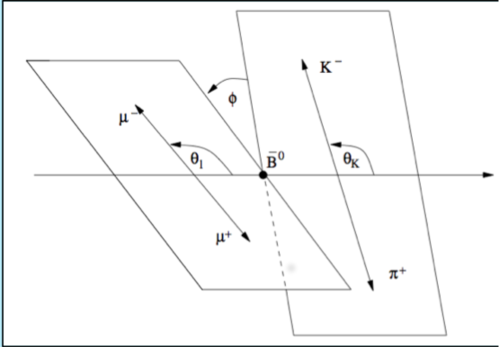
Figure 1: Graphical representation of cos$\theta_{l}$, cos$\theta_{K}$ and $\phi$. Their precise definitions are given in the text.

In [1], a long sum of products of Legendre polynomials in the concerned variables is used :

$$\epsilon\left(cos\theta_{l},cos\theta_{K},\phi,q^{2}\right)=\sum_{klmn}c_{klmn}P_{k}(cos\theta_{l})P_{l}(cos\theta_{K})P_{m}(\phi)P_{n}(q^{2}),$$ (1)

where the terms $P_{i}(x)$ stand for Legendre polynomials of order $i$. The coefficients $c_{klmn}$ are evaluated by performing a principal moment analysis of simulated ${{B}^{0}}\!\rightarrow{{K}^{*0}}(\rightarrow{{K}^{+}}{{\pi}^{-}}){\mu^{+}}{\mu^{-}}$ phase-space decays:

$$c_{klmn}=\frac{1}{N^{{}^{\prime}}}\sum_{i}^{N}\omega_{i}\left[\left(\frac{2k+1}{2}\right)\left(\frac{2l+1}{2}\right)\left(\frac{2m+1}{2}\right)\left(\frac{2n+1}{2}\right)\times P_{k}(cos\theta_{l})P_{l}(cos\theta_{K})P_{m}(\phi)P_{n}(q^{2})\right],$$ (2)

where $N$ is the total number of events and $\omega_{i}$ are weights imposed for instance to correct for known discrepancies between data and simulation. Their sum provides the total normalisation $N^{{}^{\prime}}$. For $cos\theta_{l}$, $cos\theta_{K}$, the angle $\phi$ and $q^{2}$, polynomials up to order 5, 6, 6 and 7 are used, respectively (see Ref. [1]). Designing the method, understanding the properties of the Legendre polynomials and, more generally, of the sum in Eq. 1, implementing the software to compare this parametrisation with the efficiencies observed for simulated decays so as to determine the highest orders to include until a proper description of the efficiency is obtained and to determine the $c_{klmn}$ coefficients, and interpretating the results are time demanding tasks. In the end, hundreds of $c_{klmn}$ are necessary. This might be worse in cases where more than four variables have to be dealt with, and it’s not obvious the method will always work accurately.

2.2 A new approach

The approach we propose is based on the idea that if a BDT or a NN is very powerful at detecting differences between a signal and a background sample based on a given set of $n$ variables, not by considering them individually, but by also exploiting their correlations, i.e. by comparing $n$-dimensional distributions, it should also be powerful at finding the differences between two samples differing only due to reconstruction and selection biases. In this case, instead of training the multivariate discriminator by comparing a $signal$ and a $background$ sample, one would compare samples of the same decay: an $original$ sample made of generator level decays with a $distorted$ sample made of decays that satisfied reconstruction and selection criteria. Instead of comparing discriminating variables, one would focus on the phase space of the decay, or in other words the $n$-dimensional distribution of events in the space defined by a set of independent variables that can describe fully the decay dynamics. In the example of the decay ${{B}^{0}}\!\rightarrow{{K}^{*0}}(\rightarrow{{K}^{+}}{{\pi}^{-}}){\mu^{+}}{\mu^{-}}$, this is ($q^{2}$, cos$\theta_{l}$, cos$\theta_{K}$, $\phi$).

In a four-stage approach, we first generate an original MC sample and a distorted one. The latter is generated in the same way as the former, save that reconstruction and selection cuts are applied. This stage is mandatory in most if not all physics analyses in HEP. The approaches like the ones in Sect. 2.1 need that too. When high precision is necessary one generates samples containing up to a few million events. In most HEP collaborations, generating larger samples is challenging due to limited CPU and data storage capabilities. In the test cases presented in Sect. 3 and 4, we use the ROOT package [5], and more specifically the TGenPhaseSpace class to generate these samples.

The second step is to train a multivariate analysis by comparing the samples generated above. In the case studies we carried out, we used the TMVA [4] package to train Multilayers Perceptron NNs. The only variables we provided the NNs with are the phase space variables.

The third stage is to generate additional original and distorted samples, independent of those used above for training, and to compute for each event the NN score. It summarises into one single variable all the difference detected between the original and distorted phase spaces. The reconstruction and the selection efficiency can then be parameterised in terms of only this single variable, which makes the task of accounting for this multidimensional efficiency far more practical. This is the fourth stage, where one computes the ratio of the NN score distribution obtained in the distorted sample to the distribution in the original sample. Fitting this ratio provides the parameterization, and therefore a per-candidate efficiency as a function of the score, that can be used, e.g., to weight the distorted sample so as to reproduce the phase space (and the various characteristic distributions) of the original sample.

3 Application to the study of ${{D}^{0}}\!\rightarrow{{K}^{-}}{{\pi}^{+}}{{\pi}^{+}}{{\pi}^{-}}$

Multibody ${D}^{0}$ decays provide examples where multidimensional efficiencies must be determined. These decays can be used, for instance, to improve our understanding of ${D}^{0}$ mixing [6]. One of the most studied decay is ${{D}^{0}}\!\rightarrow K^{0}_{S}{{\pi}^{+}}{{\pi}^{-}}$. Its phase space can be described in terms of two invariant masses squared: $m^{2}(K^{0}_{S}{{\pi}^{+}})$ and $m^{2}(K^{0}_{S}{{\pi}^{-}})$. The distribution of the ${{D}^{0}}\!\rightarrow K^{0}_{S}{{\pi}^{+}}{{\pi}^{-}}$ decays in the Dalitz plane [7] defined by $m^{2}(K^{0}_{S}{{\pi}^{+}})$ and $m^{2}(K^{0}_{S}{{\pi}^{-}})$ varies in time under the action of the mixing. By measuring this variation, one can access directly the mixing parameters $x=\frac{M_{1}-M_{2}}{\Gamma}$ and $y=\frac{\Gamma_{1}-\Gamma_{2}}{2\Gamma}$ [8, 9, 10], where $M_{1}$($M_{2}$), $\Gamma_{1}$($\Gamma_{2}$) and $\Gamma$ are the masses of the two neutral $D$ physical states, the two corresponding widths, and the average ${D}^{0}$ width, respectively. In simpler approaches, only a combination of $x$ and $y$ with a phase due to the strong interaction can be measured. Such Dalitz analyses also open the possibility to measure CP violation in the mixing. They can be extended to four-body decays, where the phenomenology is richer and can therefore provide more information. In this case, a five-dimensional Dalitz analysis must be carried out. Our case study in this document is the ${{D}^{0}}\!\rightarrow{{K}^{-}}{{\pi}^{+}}{{\pi}^{+}}{{\pi}^{-}}$ decay, which dynamics can be described by the following set of masses:

$$\begin{array}[]{c}m_{12}=m({{\pi}^{+}_{1}}{{\pi}^{-}})\\ m_{23}=m({{\pi}^{+}_{2}}{{\pi}^{-}})\\ m_{34}=m({{\pi}^{+}_{2}}{{K}^{-}})\\ m_{123}=m({{\pi}^{+}_{1}}{{\pi}^{-}}{{\pi}^{+}_{2}})\\ m_{234}=m({{\pi}^{-}}{{\pi}^{+}_{2}}{{K}^{-}}).\\ \end{array}$$

3.1 Generation of the distorted and original samples

We generated an original sample and a distorted sample of ${{D}^{0}}\!\rightarrow{{K}^{-}}{{\pi}^{+}}{{\pi}^{+}}{{\pi}^{-}}$ decays. Both contain $\sim$ 230000 decays. A sample of reconstructed and selected events of this size is a significant computing effort if a full simulation (physics, detector response and reconstruction) has to be performed. However, this is still in the scope of what a collaboration like LHCb, the present world leading experiment in Flavor Physics [11], is ready to produce even for measurements of intermediate importance.

To produce samples that can be compared with the samples used by LHCb in [12], an important element is to generate decays that have the same kinematics as in LHCb’s laboratory frame. This is not possible with the TGenPhaseSpace class alone, which knows nothing of the physics of the proton-proton collision where $D^{0}$ mesons are produced. Using this class one can generate the four-momentum of each daughter particles given the four-momentum of the decaying particle, assuming a flat phase space ( i.e. assuming that all the combinations of daughter four-momenta that respect energy and momentum conservation are equally allowed). To reproduce the kinematics of ${D}^{0}$ mesons produced in proton-proton collisions at a center-of-mass energy of 7 or 8 TeV, we combined several samples, each generated assuming a different value of the ${D}^{0}$ transverse momentum and rapidity. The relative contribution of each sample to the final one was decided according the ${D}^{0}$ production cross sections measured in Ref. [13] as a function of these quantities. This is how the original sample was produced.

To produce the distorted sample, we first generated decays as described above, and filtered them according to a selection which aims to be as close as possible to the selection used in Ref. [12]. At LHCb, the selection of a given $M$ meson decay typically involves:

• The momentum ($p$) and transverse momentum ($p_{\mathrm{T}}$) of the mother and daughter particles.

• The minimum distance of a track to a proton-proton primary vertex (PV), called the impact parameter (IP).

• The difference in $\chi^{2}$ of the closest PV reconstructed with and without the particle under consideration ($\chi^{2}_{\mathrm{IP}}$). This particle can either be $M$ or one of its decay products.

• The $\chi^{2}$ evaluating the quality of the $M$ decay vertex ($\chi^{2}_{\mathrm{Vtx}}$).

• The invariant mass of the $M$ candidate $m(M)$.

• The angle between the $M$ momentum and the line joining the PV and the decay vertex of $M$ (DIRA), which has to be consistent with zero to ensure the $M$ candidate originates from the PV.

• The significance of the distance between the $M$ decay vertex and the PV ($\chi^{2}_{\mathrm{FD}}$).

• The reconstructed lifetime $\tau_{M}$.

• Variables describing the isolation of the final state tracks.

• Statistical estimators of the nature of the decay products, which combine the information from LHCb’s RICH, calorimeters and muon system (PID($\pi$), ProbNNmu).

In the present study, only the generation phase is simulated. Therefore, only the “true”, generator-level, $p$ and $p_{\mathrm{T}}$ of the ${D}^{0}$ and decay products are available in our samples, and the selection we apply to produce a realistic distorted sample relies only on these variables. We checked that the distortion we introduced in the phase space is consistent with that observed in the analysis presently carried out by LHCb [12], even though we can use only the true information, rather than the reconstructed one, and no information on vertexing nor on decay topology. To achieve this, some cuts on momenta and transverse momenta are tightened with respect to the selection in [12]. We require all the decay products to be in the acceptance of the LHCb detector (i.e. the angle between their momentum and the nominal beam line should lie in the range 0.01-0.4 rad), and the candidates must satisfy the following criteria :

• $p_{\mathrm{T}}(D^{0})>3$ GeV$/c$.

• $p_{\mathrm{T}}>0.5$ GeV$/c$, $p>3$ GeV$/c$ for all the decay products.

• max($p(K^{-}),p(\pi^{+}),p(\pi^{+}),p(\pi^{-})$)$>10$ GeV$/c$.

• max($p_{\mathrm{T}}(K^{-}),p_{\mathrm{T}}(\pi^{+}),p_{\mathrm{T}}(\pi^{+}),p_{\mathrm{T}}(\pi^{-})$)$>1.7$ GeV$/c$.

• max($p_{\mathrm{T}}(K^{-}),p_{\mathrm{T}}(\pi^{+}),p_{\mathrm{T}}(\pi^{+}),p_{\mathrm{T}}(\pi^{-})$)$>3.7$ GeV$/c$ with the hardware trigger reconstruction.

By construction, the generator-level $p$ and $p_{\mathrm{T}}$’s available in our samples do not account for the finite resolution of the reconstruction. Since in LHCb the momentum resolution of the offline reconstruction is very small (from 0.5% at low momentum to 1% at 200 GeV$/c$), we consider that we can safely neglect it. One expection is made for the first stage of LHCb’s trigger system. It’s a hardware trigger that searches for high $p_{T}$ objects, based on a partial event reconstruction carried out by the Front End electronics [14]. Several kinds of objects are searched for, involving several trigger $lines$: candidates are looked for in the muons system, while in the electromagnetic calorimeter clusters due to photons or electrons are sought. In the case of a decay like ${{D}^{0}}\!\rightarrow{{K}^{-}}{{\pi}^{+}}{{\pi}^{+}}{{\pi}^{-}}$, the hardware trigger looks for high $p_{T}$ clusters ($>$ 3.7 GeV$/c$) in the Hadron Calorimeter, which resolution is $\sigma_{E}/E=80\%/\sqrt{E}\oplus 10\%$ with $E$ expressed in GeV. We apply the trigger cut to particles which $p_{T}$ has been smeared in order to reproduce this resolution. This trigger cut is applied to only a third of the events since LHCb events in which a ${{D}^{0}}\!\rightarrow{{K}^{-}}{{\pi}^{+}}{{\pi}^{+}}{{\pi}^{-}}$ decay is produced are often triggered on independently, due to the decay products of the second charm hadron produced in the event (proton-proton collisions actually produce $c-\bar{c}$ $pairs$).

On Fig. 2 we compare the distributions of $m_{12},~{}m_{23},~{}m_{34},~{}m_{123}$ and $m_{234}$ in the distorted and original samples. The selection efficiencies as a function of each of these variables (i.e., the ratio between the distributions superimposed on Fig. 2) are also shown on Fig. 3. This illustrates the effect of the selection on the phase space.

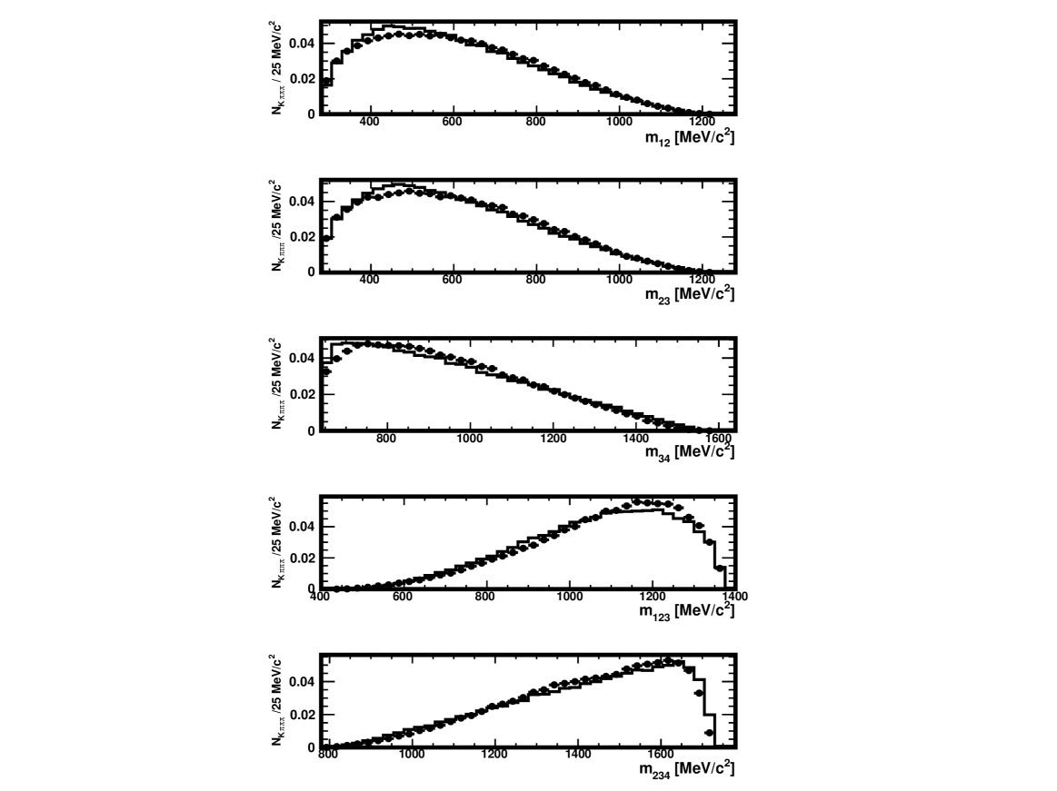
Figure 2: Distributions of $m_{12}$, $m_{23}$, $m_{34}$, $m_{123}$ and $m_{234}$ in the original sample (histogram) and in the distorted one (full circles). The normalisation is arbitrary.

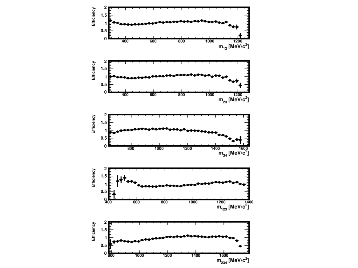
Figure 3: Efficiency in $m_{12}$, $m_{23}$, $m_{34}$, $m_{123}$ and $m_{234}$ observed in the data generated for this study. Shown are the ratios of the distributions found in the distorted and original samples. The normalisation of these distributions was arbitrary.

3.2 Neural network training

We chose to use the MLPBNN NN provided by the TMVA package. This Multilayer Perceptron (MLP) NN is trained using the BFGS method instead of a simple back-propagation method. The definition of a MLP, and a description of the latter method can be found in Ref. [4]. Also, a Bayesian regulation technique is employed. It is described in Ref. [15]. We used the default configuration found in the example macro downloaded with the TMVA package. To the attention of the expert reader, we specify that in this case the MLP involves only one hidden layer, which comprises $N+10$ neurons, where $N$ is the number of input variables ($m_{12},~{}m_{23},~{}m_{34},~{}m_{123}$ and $m_{234}$ in our case). The neuron activation function is $tanh$. Input variables are linearly scaled to lie with $\mathrm{\left[-1;1\right]}$, and 600 training cycles are performed. An overtraining test is run every 5 cycles. All the other settings can be found in Table 19 of Ref. [4].

It took two hours to train this MLP to distinguish between decays from the distorted or original samples (both contain 230000 events). We used a machine equipped with a Intel i7-640M 2.8 GHz 2-Core processor. Two additional distorted and original samples, produced in the same way as those used for training, and of identical size, have been produced to test the resulting NN score. The distribution of this score in both samples is shown on Fig. 4, which also displays the ratio these distributions, to which we fitted a parameterised efficiency, $\epsilon\left(s\right)$, where $s$ is the NN score. We used for that a fifth order polynomial. The $\epsilon\left(s\right)$ function should match $\epsilon\left(m_{12},m_{23},m_{34},m_{123},m_{234}\right)$, the multidimensional efficiency we aim at.

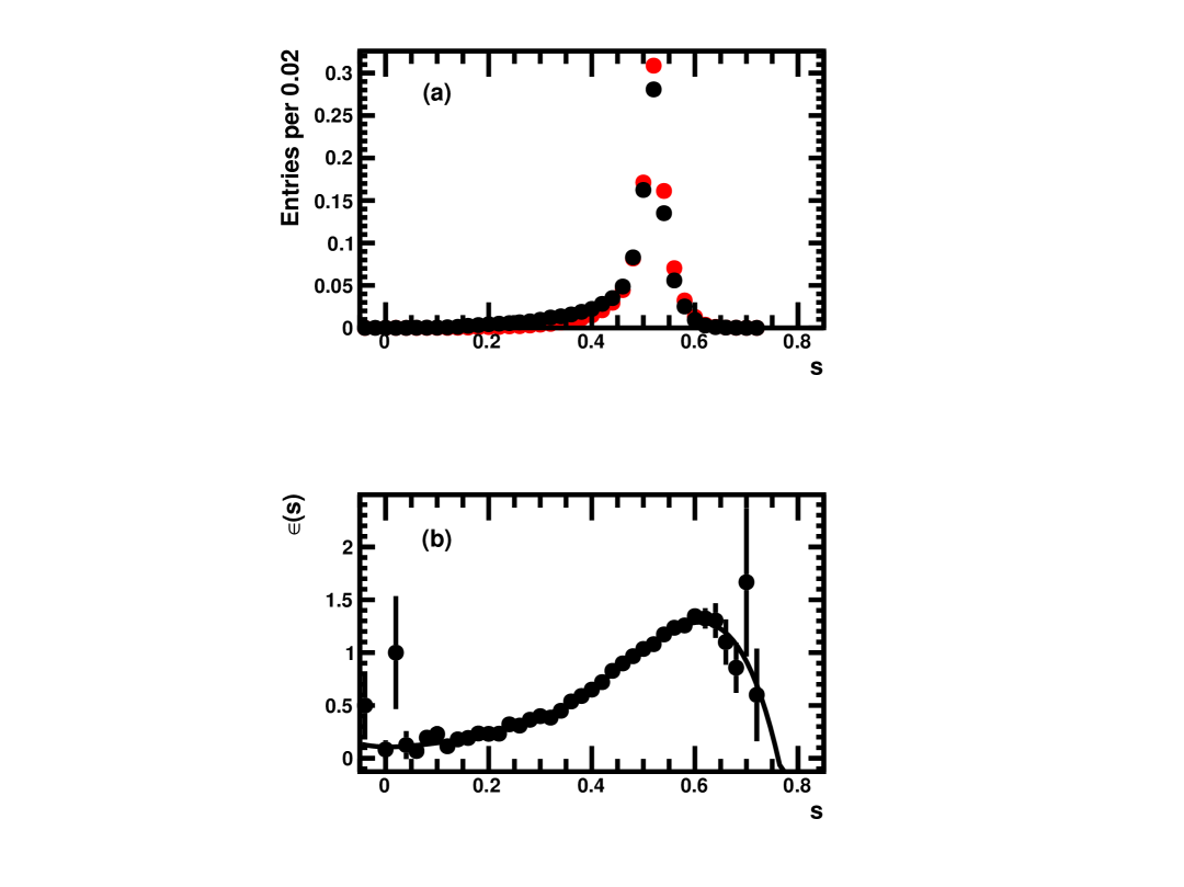
Figure 4: Distributions and distribution ratio showing (a) the NN score $s$ in the distorted (red) and original (black) ${{D}^{0}}\!\rightarrow{{K}^{-}}{{\pi}^{+}}{{\pi}^{+}}{{\pi}^{-}}$ samples, and (b) the selection efficiency as a function of $s$ (with an arbitrary normalisation). The fit leading to $\epsilon(s)$ is superimposed to the measured efficiencies.

3.3 Results

To test the efficiency obtained above, we weighted each ${{D}^{0}}\!\rightarrow{{K}^{-}}{{\pi}^{+}}{{\pi}^{+}}{{\pi}^{-}}$ decay $i$ in the distorted test sample with $\omega_{i}=1/\epsilon\left(s_{i}\right)$. The result can be found in Fig. 5. It is the same as Fig. 2 with distributions from the re-weighted distorted sample superimposed. One can see that these distributions match closely those observed in the original sample, before the distortions due to the selection were imposed. The ratios on Fig. 6 are consistent with 1 all over the $m_{12},~{}m_{23},~{}m_{34},~{}m_{123}$ and $m_{234}$ spectra, unlike the un-weighted ratios on Fig. 3, which show clear distortions.

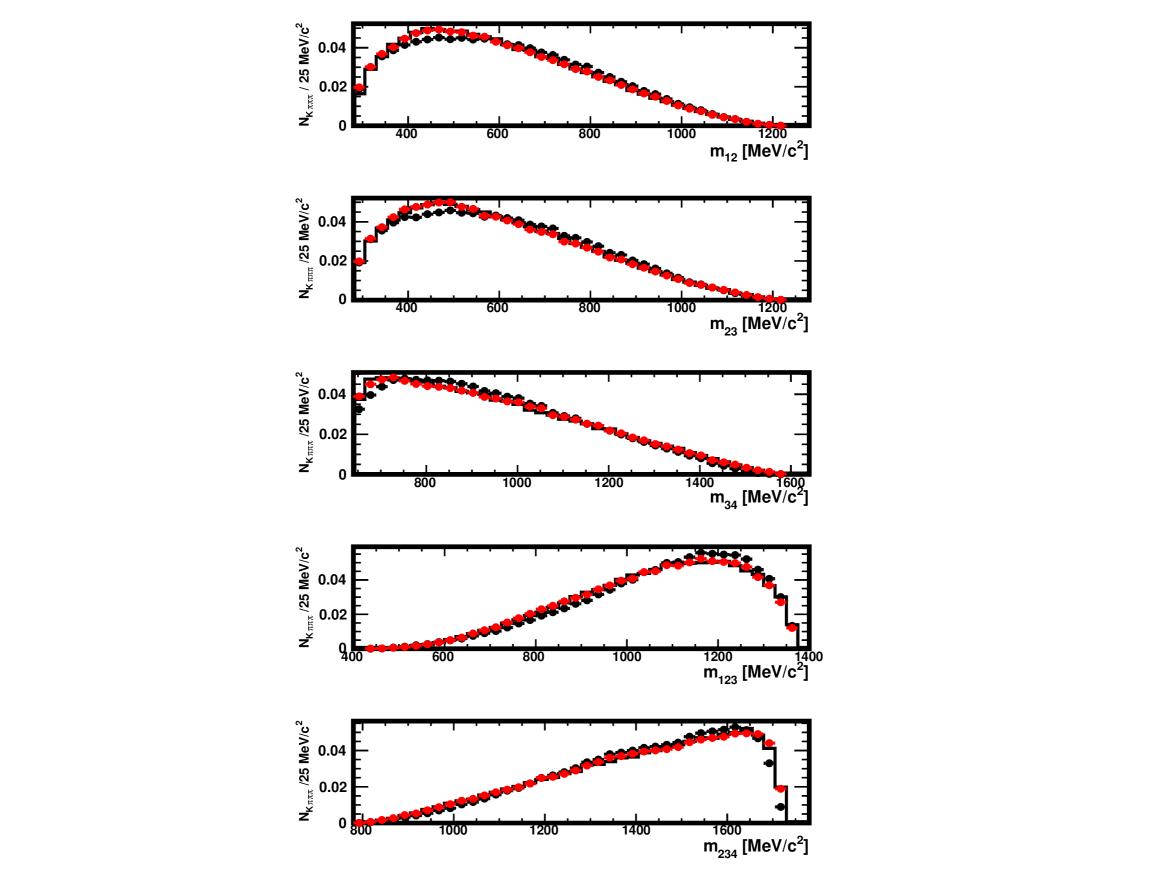
Figure 5: Distributions of $m_{12}$, $m_{23}$, $m_{34}$, $m_{123}$ and $m_{234}$ in the original sample (histogram), in the distorted one (full black circles) and in the distorted sample where the decays have been re-weighted using the $\omega_{i}$ weights (red), as explained in the text. The absolute normalisation is arbitrary when the correction is not applied and natural when it is applied (red).

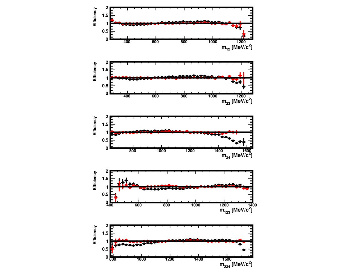
Figure 6: Efficiency in $m_{12}$, $m_{23}$, $m_{34}$, $m_{123}$ and $m_{234}$ in the data generated for this study. Shown are the ratios of the distributions found in the distorted and original samples, with no correction (black) and for decays re-weighted using $\omega_{i}$ weights (red) as explained in the text. The absolute normalisation is arbitrary when the correction is not applied and natural when it is applied (red).

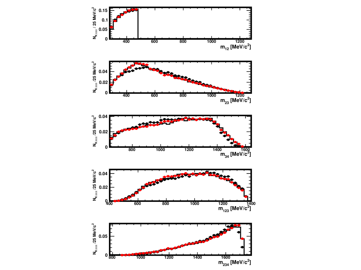
Figure 16: Distributions of $m_{12}$, $m_{23}$, $m_{34}$, $m_{123}$ and $m_{234}$ in the original sample (histogram), in the distorted one (full black circles) and in the distorted sample where the decays have been re-weighted using the $\omega_{i}$ weights (red), as explained in Sect. 3.3. The data used here are restricted to the region $0<m_{12}<480$ MeV$/c^{2}$. The absolute normalisation is arbitrary when the correction is not applied and natural when it is applied (red).

Consequently, the MLP we trained produces a single variable $s$ to fully encompass the 5-dimensional information on the distortion of the ($m_{12},m_{23},m_{34},m_{123},m_{234}$) space. The $\epsilon\left(s\right)$ efficiency accounts simultaneously for the 5 individual efficiencies as a function of $m_{12},~{}m_{23},~{}m_{34},~{}m_{123}$ and $m_{234}$. The yield in each bin of the corrected distributions in Fig. 5 is calculated as the sum of the $\omega_{i}$ weights over all the events that lie in this bin. In principle, this corrected yield can be correct even if $\epsilon\left(s\right)$ is not an accurate evaluation of $\epsilon\left(m_{12},m_{23},m_{34},m_{123},m_{234}\right)$ everywhere in the $\left(m_{12},m_{23},m_{34},m_{123},m_{234}\right)$ space. A compensation is possible in the sum. Also, the evaluation could be wrong in regions containing too little statistics for the effect to appear significantly on Figs. 5 and 6. To constrain this possibility, we repeated the test of Figs. 5 and 6 in various restricted regions of the $\left(m_{12},m_{23},m_{34},m_{123},m_{234}\right)$ space. The results are on Figs. 16 to 55 of Appendix A. The corrected distributions once more match the original ones. Note that we still use the efficiency from Fig. 4 for these corrections. The polynomial’s parameters were not re-evaluated by performing in each region specific fits or new trainings. We conclude that $\epsilon\left(s\right)$ = $\epsilon\left(m_{12},m_{23},m_{34},m_{123},m_{234}\right)$, in the limit of the precision with which it can be verified with our data.

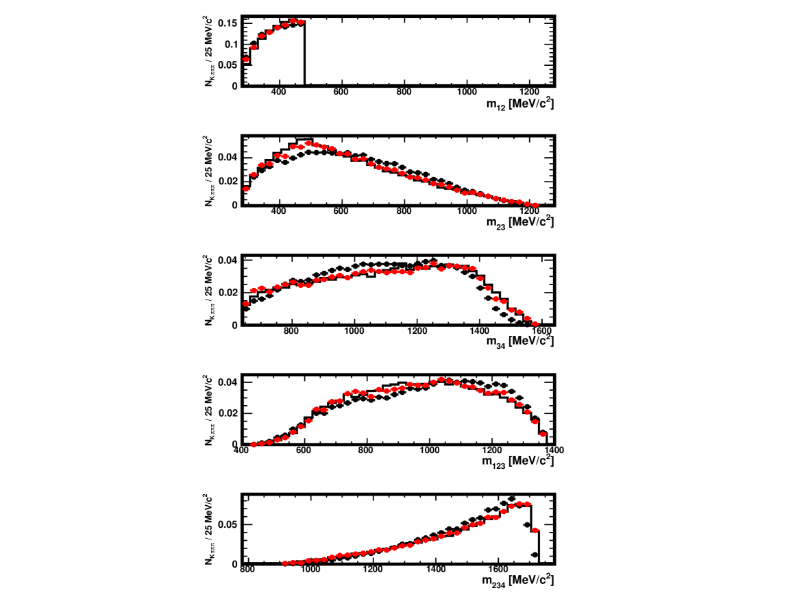
Figure 56: Distributions of $m_{12}$, $m_{23}$, $m_{34}$, $m_{123}$ and $m_{234}$ in the original sample (histogram), in the distorted one obtained with a tighter selection (full black circles) and in the distorted sample where the decays have been re-weighted using the $\omega_{i}$ weights (red), as explained in Sect. 3.3. The data used here are restricted to the region $0<m_{12}<480$ MeV$/c^{2}$. The absolute normalisation is arbitrary when the correction is not applied and natural when it is applied (red).

We reach the same conclusion when applying the same technique to correct an alternative distorted sample, obtained with tighter cuts and therefore showing stronger distortions in the phase space. We tightened one cut on the ${{D}^{0}}\!\rightarrow{{K}^{-}}{{\pi}^{+}}{{\pi}^{+}}{{\pi}^{-}}$ decay products: $p_{\mathrm{T}}>0.6$ GeV$/c$. Also, the hardware trigger selection is applied to all events instead of only a third. The results we obtained can be judged with the help of Figs. 7 and 8. What we obtained in particular regions of the phase space is shown on Figs. 56 to 95 in Appendix A.

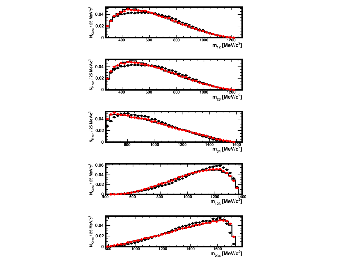
Figure 7: Distributions of $m_{12}$, $m_{23}$, $m_{34}$, $m_{123}$ and $m_{234}$ in the original sample (histogram), in the distorted one obtained with a tighter selection (full black circles) and in the same sample where the decays have been re-weighted using the $\omega_{i}$ weights (red), as explained in the text. The absolute normalisation is arbitrary when the correction is not applied and natural when it is applied (red).

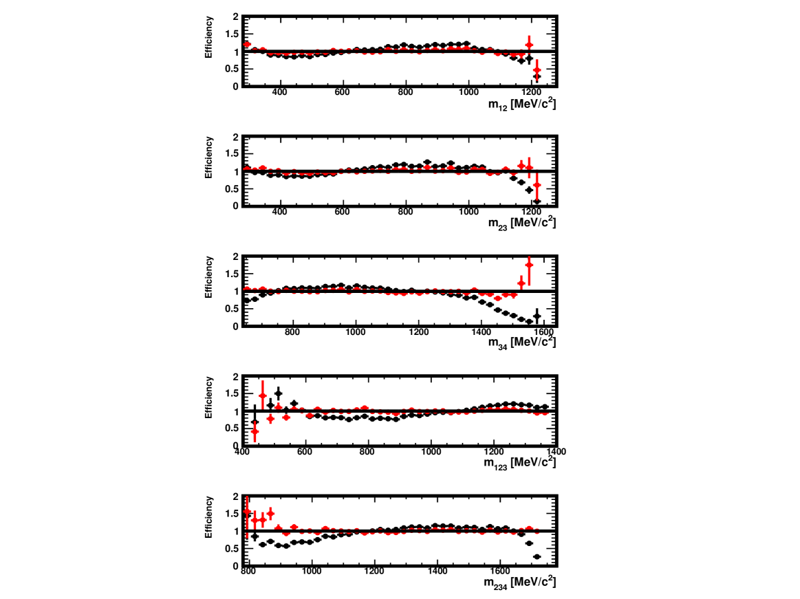
Figure 8: Efficiency in $m_{12}$, $m_{23}$, $m_{34}$, $m_{123}$ and $m_{234}$ in the data generated for this study, with a tighter selection for the distorted sample. Shown are the ratios of the distributions found in the distorted and original samples, with no correction (black) and for decays re-weighted using $\omega_{i}$ weights (red) as explained in the text. The absolute normalisation is arbitrary when the correction is not applied and natural when it is applied (red).

4 Application to the study of ${{B}^{0}}\!\rightarrow{{K}^{*0}}(\rightarrow{{K}^{+}}{{\pi}^{-}}){\mu^{+}}{\mu^{-}}$

We performed a second case study to explore the potential of MVAs to treat multidimensional efficiencies. It is based on the decay ${{B}^{0}}\!\rightarrow{{K}^{*0}}(\rightarrow{{K}^{+}}{{\pi}^{-}}){\mu^{+}}{\mu^{-}}$. A similar procedure to that described in Sect. 3 has been carried out for that purpose.

4.1 Sample generation

We generated a distorted and an original sample, both containing 600 000 decays. This is less than in the sample used by the LHCb collaboration for the result in Ref. [1]. Because the study of this mode is one of LHCb’s priorities, it was actually acceptable produce as much as 1.406M reconstructed and selected events.

The ROOT TGenPhaseSpace class is used once more to generate decays. The kinematics of the $B^{0}$ meson is derived from the differential production cross-section as a function of transverse momentum and rapidity, measured in proton-proton collisions at a center-of-mass energy of 7 TeV [16].

To produce the distorted sample, we applied a selection as similar as possible to that in [1]. The following criteria are used:

• All the decay products must be in the acceptance of the LHCb detector.

• One of the muons should satisfy $p_{\mathrm{T}}(\mu)>1.8$ GeV$/c$ in order to reproduce the cut used by the muon-specific line which dominates the hardware trigger in the case of decays such as ${{B}^{0}}\!\rightarrow{{K}^{*0}}(\rightarrow{{K}^{+}}{{\pi}^{-}}){\mu^{+}}{\mu^{-}}$.

• max($p(K^{+}),p(\pi^{-}),p(\mu^{+}),p(\mu^{-})$)$>10$ GeV$/c$.

• max($p_{\mathrm{T}}(K^{+}),p_{\mathrm{T}}(\pi^{-}),p_{\mathrm{T}}(\mu^{+}),p_{\mathrm{T}}(\mu^{-})$)$>0.2$ GeV$/c$.

• $p_{\mathrm{T}}(B^{0})>4$ GeV$/c$.

• $p(B^{0})>40$ GeV$/c$.

• max($IP(K^{+}),IP(\pi^{-}),IP(\mu^{+}),IP(\mu^{-})$)$>1$ mm.

• For all decay products, $\chi^{2}_{\mathrm{IP}}>9$.

Only momenta and transverse momenta are directly accessible in the data generated with the TGenPhaseSpace class. The cuts on these variables, even tighter than those in [1], could not reproduce the distortion of the phase space variables actually observed in this analysis (Fig. 9). This was true in particular of the acceptance as a function of $\phi$, which was flatter. In the hope to reproduce a comparable distortion, we included cuts that affect angular variables more directly. This is the reason of the presence of cuts on $IP$ and $\chi^{2}_{\mathrm{IP}}$ in the above list. The $IP$ was determined based on the angle between the ${{B}^{0}}\!\rightarrow{{K}^{*0}}(\rightarrow{{K}^{+}}{{\pi}^{-}}){\mu^{+}}{\mu^{-}}$ decay products and the momentum of the $B^{0}$, assuming the latter travelled a typical 8 mm before its decay. We approximated $\chi^{2}_{\mathrm{IP}}$ by the squared ratio between $IP$ and its uncertainty. The latter was computed based on the transverse momentum of the particle under consideration and on the typical uncertainty observed in LHCb. We used the uncertainty advertised by LHCb in recent publications (see for instance [1]), $\sigma_{IP}=(15+29/\mbox{$p_{\rm T}$}){\,\upmu\rm m}$ with $p_{\rm T}$ in GeV$/c$. These cuts did not yet suffice to reproduce the amplitude of the distortion in the $\phi$ distribution. We obtained this by discarding decays which do not satisfy $\left|m(K\pi)-892\right|>0.09\times\left(q^{2}/(19.10^{6})\mathrm{sin^{2}}(\phi)\times 100\right)$ where $m(K\pi)$ and $q$ are expressed in MeV$/c^{2}$. With this set of criteria, the distortion of the ($q^{2}$, cos$\theta_{l}$, cos$\theta_{K}$, $\phi$) space, although not idenditical, is similar to that observed in Ref. [1]. This can be seen in on Figs. 10 and 11, which show the distortion in our generated data, in extreme regions of $q^{2}$: $0.1<q^{2}<0.98$ GeV${}^{2}/c^{4}$ and $18.0<q^{2}<19.0$ GeV${}^{2}/c^{4}$. They can be compared with Fig. 9 to notice that the evolution of the distortion between these two regions is reproduced. We checked that the same conclusion holds in all $q^{2}$ regions by comparing Figs. 96 to 114 (see Appendix B) with the equivalent figures in [17].

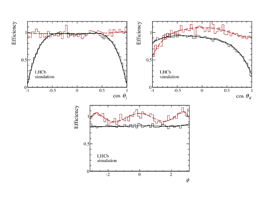
Figure 9: Angular efficiency in cos$\theta_{l}$, cos$\theta_{K}$ and $\phi$, as determined from a principal moment analysis of simulated three-body ${{B}^{0}}\!\rightarrow{{K}^{*0}}(\rightarrow{{K}^{+}}{{\pi}^{-}}){\mu^{+}}{\mu^{-}}$ phase-space decays (black solid and red long-dashed lines), and compared to simulated data (histograms). The efficiency is shown for the regions: $0.1<q^{2}<0.98$ GeV${}^{2}/c^{4}$ (black) and $18.0<q^{2}<19.0$ GeV${}^{2}/c^{4}$ (red). The absolute normalisation is arbitrary. This figure is reproduced from Ref. [1].

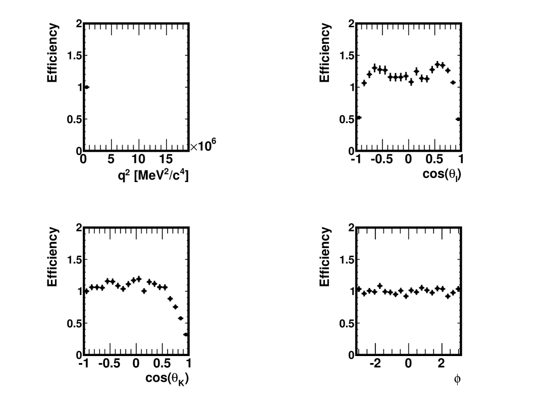
Figure 10: Efficiency in $q^{2}$, cos$\theta_{l}$, cos$\theta_{K}$ and $\phi$ in the data generated for the present study, in the region $0.1<q^{2}<0.98$ GeV${}^{2}/c^{4}$. The absolute normalisation is arbitrary.

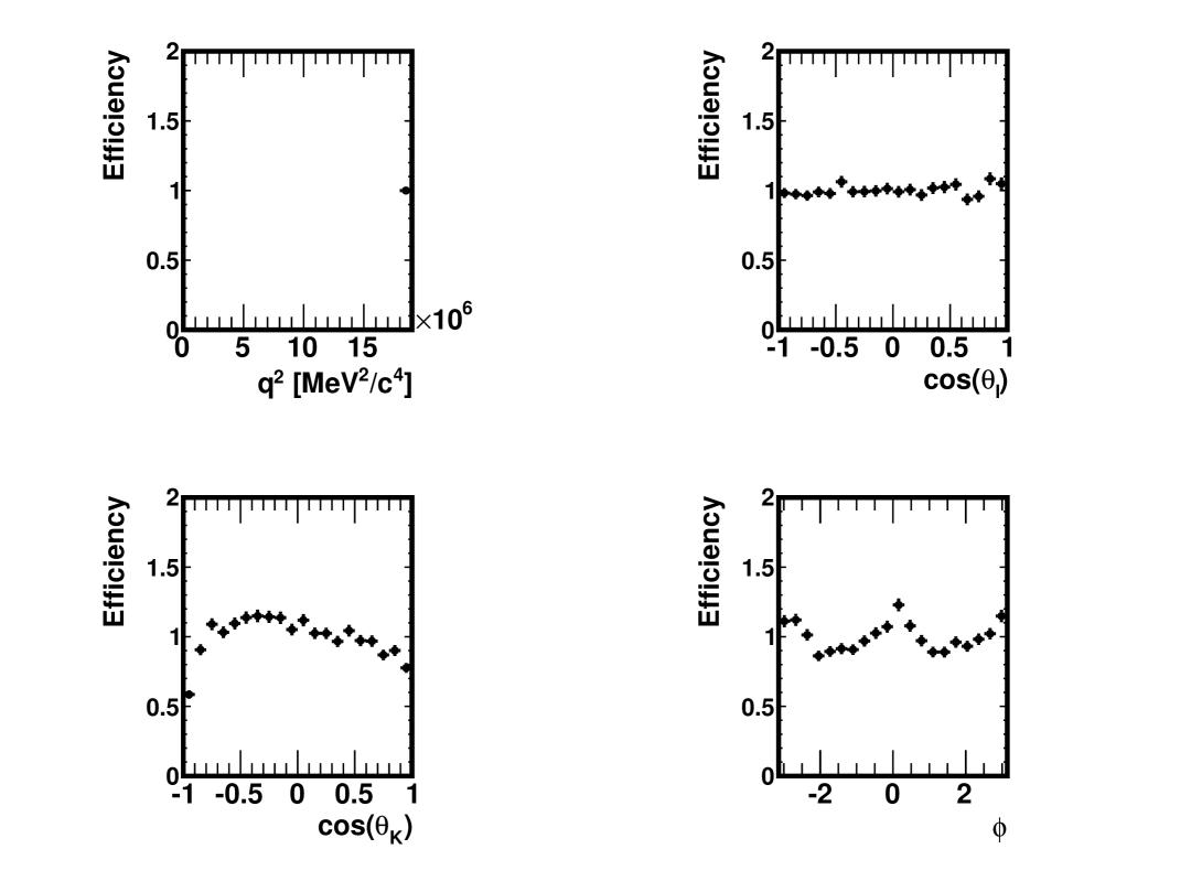
Figure 11: Efficiency in $q^{2}$, cos$\theta_{l}$, cos$\theta_{K}$ and $\phi$ in the data generated for the present study, in the region $18.0<q^{2}<19.0$ GeV${}^{2}/c^{4}$. The absolute normalisation is arbitrary.

4.2 Neural network training

We trained the MLP NN provided by the TMVA package. It is the same NN as that described in Sect. 3, modulo two differences: the classical back-propagation technique described in [4] is used instead of the BFGS method, and we use no Bayesian regulation technique.

The distortion of the ($q^{2}$, cos$\theta_{l}$, cos$\theta_{K}$, $\phi$) space is more challenging to correct as that of the ($m_{12},~{}m_{23},~{}m_{34},~{}m_{123}$, $m_{234}$) space in the previous section. Indeed, as can be seen on Figs. 9, 10 and 11, the distortion the cos$\theta_{l}$ and $\phi$ distributions is symmetric in these variables. As a consequence, the discriminative power of these variables is low: the distorted and original samples cannot be distinguished via a strong “preference” of one of them for the higher or the lower end of the cos$\theta_{l}$ or $\phi$ distributions. In other words, the efficiencies with which distorted and original events would be selected by a cut on cos$\theta_{l}$ or $\phi$ would not differ nor vary much as a function of the value of this cut. Another difficulty complicates the determination of the multidimensional efficiency $\epsilon\left(q^{2},cos\theta_{l},cos\theta_{K},\phi\right)$ with the approach presented in this document. It stems from the fast variation as a function of $q^{2}$ of the distortion in the 3 other variables and the particular pattern it follows: at low $q^{2}$, the distortion is strong in cos$\theta_{l}$ and very light in $\phi$, while the opposite is observed at high $q^{2}$ (this pattern can be seen again on Figs. 9, 10 and 11). There is therefore a more complicated structure to be understood by the NN. Also, the fact that in some regions in $q^{2}$ only two variables are available to discrimate the distorted sample against the original one is a difficulty in itself. Moreover, it is not trivial for the NN to adapt to this varying behavior since it is trained using the whole distorted and original samples. It is not instructed to treat differently the various $q^{2}$ regions. This difficulty affects the determination of $\epsilon\left(q^{2},cos\theta_{l},cos\theta_{K},\phi\right)$ in the whole sample and becomes more acute when it comes to determine the multidimensional efficiency in restricted regions of $q^{2}$.

To overcome these difficulties, the input variables mapped to the NN’s first layer are not directly $q^{2}$, cos$\theta_{l}$, cos$\theta_{K}$, and $\phi$. We replace cos$\theta_{l}$ and $\phi$ by two transformed, non-symmetric variables: $e^{-\theta_{l}^{2}/4}$ and $e^{-\mathrm{sin}^{2}(\phi)/4}$. Also, unlike in Sect. 3, we had to optimise the NN settings instead of using blindly the ones provided by default by TMVA. We devoted a limited effort (a day of work) to this. In practice :

• We further transformed the input variables so as to make their distributions gaussian, which helps the decorrelation algorithms used by the NN [4].

• We used two hidden layers instead of only one. The number of neurons constituting the first and second layers is 14 and 6, respectively. It has to be compared with 4, the number of input variables.

• The number of training cycle was raised to 7000.

• Overtraining tests were run every 5 cycles. Each time, the convergence is also tested. If 10 consecutive tests fail to observe an improvement of the error function, the training is considered optimal and stopped.

All the other settings can be found in Table 19 of Ref. [4]. With these settings, it took $\sim$12 hours to train the NN on the same machine as in Sect. 3.

4.3 Results

We show on Fig. 12 the distribution of the NN score $s$ obtained in original and distorted test samples, generated independently from the training samples. This figure also shows $\epsilon\left(s\right)$, the parameterised efficiency fitted to the ratio of the original and distorted distributions. We tested this efficiency in the same way as in Sect. 3.3. Fig. 13 shows the efficiency in $q^{2}$, cos$\theta_{l}$, cos$\theta_{K}$ and $\phi$. Also shown are the efficiencies obtained with the corrected distorted sample, in which each decay $i$ is weigted by $\omega_{i}=1/\epsilon\left(s_{i}\right)$. The corrections works precisely: in no bin does the latter ratio differ from 1 by more than a few percents. This difference is never statiscally significant. The latter statement also holds in specific regions of the $q^{2}$ distribution, as can be seen on Fig. 14, which shows this efficiency in the region $0.1<q^{2}<0.98$ GeV${}^{2}/c^{4}$ and on Fig. 15 which focusses on the region $18.0<q^{2}<19.0$ GeV${}^{2}/c^{4}$. This can be compared to what was obtained by the analysis reported in [1] (Fig. 9), with the principal moment analysis briefly described in Sect. 2.1. The correction we obtained is less precise statistically — which is natural with more than twice less statistics — but is of comparable accuracy. This is a promising result since it was obtained with very limited efforts and MVA-related competences. The quality of the correction was confirmed in 19 $q^{2}$ regions, as can be seen on Figs. 96 to 114 in Appendix B. We remind that in each $q^{2}$ region the weights are still calculated from the $\epsilon\left(s\right)$ function fitted to the efficiency shown on Fig. 12. No specific training and no re-evaluation of the polynomial is performed in individual regions.

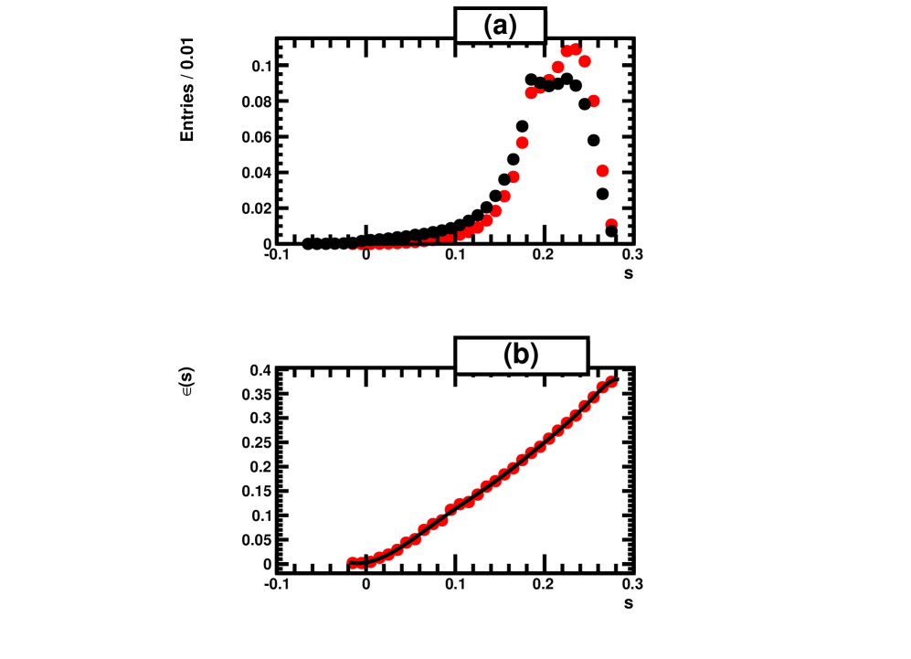
Figure 12: Distributions and distribution ratio showing (a) the NN score $s$ in the distorted (red) and original (black) ${{B}^{0}}\!\rightarrow{{K}^{*0}}(\rightarrow{{K}^{+}}{{\pi}^{-}}){\mu^{+}}{\mu^{-}}$ samples, and (b) the selection efficiency as a function of $s$ (with an arbitrary normalisation). The fit providing to $\epsilon\left(s\right)$ is superimposed to the measured efficiencies.

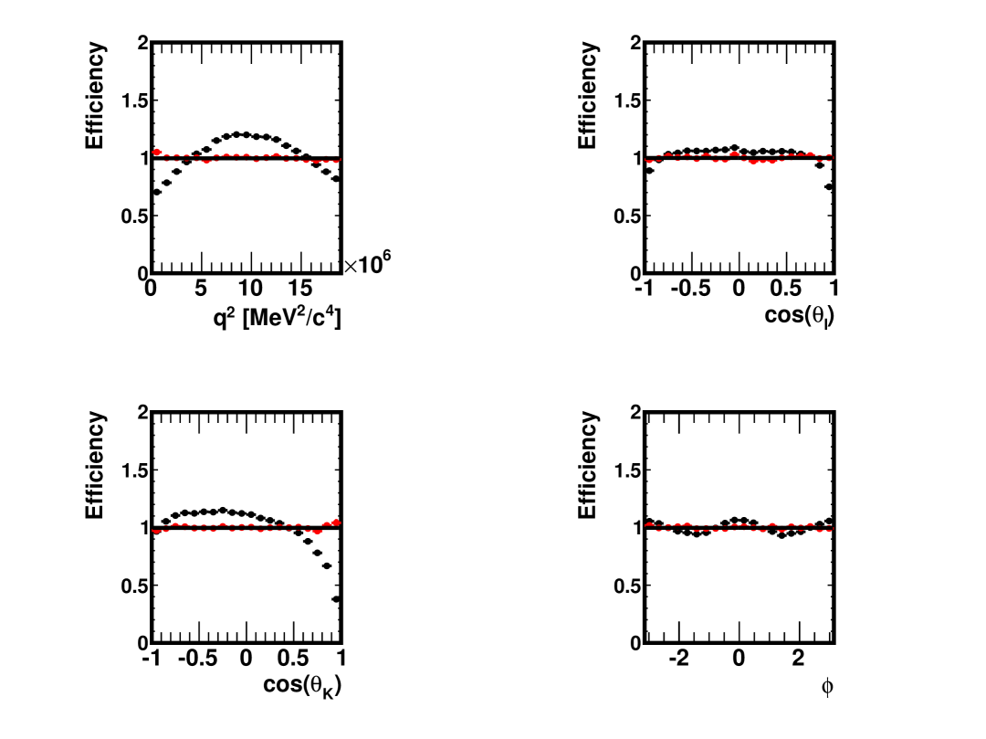
Figure 13: Efficiency in $q^{2}$, cos$\theta_{l}$, cos$\theta_{K}$ and $\phi$ in the data generated for the present study. Shown are the ratios of the distributions found in the distorted and original samples, with no correction (black) and for decays re-weighted using $\omega_{i}$ weights (red) as explained in the text. The absolute normalisation is arbitrary when the correction is not applied, natural when it is (red).

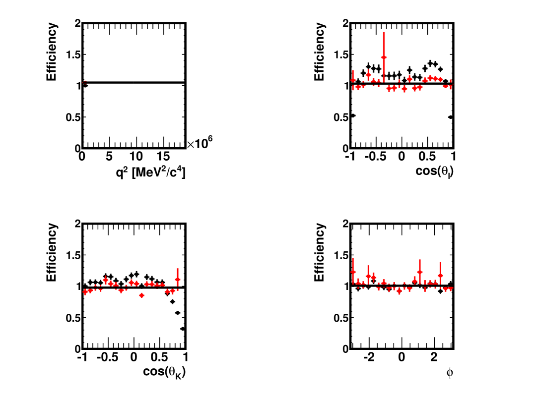
Figure 14: Efficiency in $q^{2}$, cos$\theta_{l}$, cos$\theta_{K}$ and $\phi$ in the data generated for the present study, in the region $0.1<q^{2}<0.98$ GeV${}^{2}/c^{4}$. Shown are the ratios of the distributions found in the distorted and original samples, with no correction (black) and for decays re-weighted using $\omega_{i}$ weights (red) as explained in the text. The absolute normalisation is arbitrary when the correction is not applied, natural when it is (red).

Figure 15: Efficiency in $q^{2}$, cos$\theta_{l}$, cos$\theta_{K}$ and $\phi$ in the data generated for the present study, in the region $18.0<q^{2}<19.0$ GeV${}^{2}/c^{4}$. Shown are the ratios of the distributions found in the distorted and original samples, with no correction (black) and for decays re-weighted using $\omega_{i}$ weights (red) as explained in the text. The absolute normalisation is arbitrary when the correction is not applied, natural when it is (red).

As in Sect. 3, we conclude the $\epsilon\left(s\right)$ obtained with the approach proposed in this document can be used to evaluate the effiency at a given point of the decay phase space.

5 Conclusion

We proposed a novel approach to the determination of multidimensional efficiencies and explored its potential with two realistic examples, typical of the need of modern Heavy Flavor physics measurements. We used Neural Networks to characterize the differences introduced in a 4 or 5-dimensional phase space by typical reconstruction and selecion criteria. These tools were trained and tested using simulated samples of similar size to that of the samples used by the LHCb collaboration for published (or soom published) measurements of the decay modes ${{D}^{0}}\!\rightarrow{{K}^{-}}{{\pi}^{+}}{{\pi}^{+}}{{\pi}^{-}}$ and ${{B}^{0}}\!\rightarrow{{K}^{*0}}(\rightarrow{{K}^{+}}{{\pi}^{-}}){\mu^{+}}{\mu^{-}}$. In both test cases studied in this document, the NN score allows to correct the selected samples in order to reproduce the phase space distributions observed in samples that have not undergone any selection. This is an evidence the approach developped here allows to evaluate the efficiency at any point of a multidimensional phase space. Compared to elaborate techniques like the principal moment method used in [1], this new appraoch seems less precise statistically although as accurate. It would probably suffice for many measurements that do not require the same level of precision as the angular analysis of ${{B}^{0}}\!\rightarrow{{K}^{*0}}(\rightarrow{{K}^{+}}{{\pi}^{-}}){\mu^{+}}{\mu^{-}}$ reported in [1]. In such cases, it would represent a considerable gain of working time since satisfactory results can be achieved with minimum skills and knowledge of MVA techniques, using packages already routinely used within the HEP community, with no need of any elaborate optimisation nor of more than a few days of work and a few hours of CPU consumption. This is the conclusion of this study. It also suggests that with more expertise and cutting-edge MVA techniques, a precise treatment of multidimensional efficiencies is possible and could be applied to measurements of primary importance.

Other applications of MVAs to HEP, besides signal vs. background discrimination, can be considered in the future. Selection efficiencies often rely on simulations that match real data only imperfectly and require systematic Data/MC comparisons to correct the simulation. When the correction must be applied to many variables, using a MVA to compare data with MC and derive “automatically” a unique number to reweight the simulation would be a valuable tool.

In a given analysis, if one knows the efficiency at each point of the phase space, the signal events found in data can be corrected to obtained the distributions of interest before any selection bias, without having to use an imperfect simulation. This is not possible in cases where a rare decay is searched for. There, very few signal events are found, if any, and there is nothing to re-weight. The technique proposed in this document could be used to guide the selection design in order to obtain a flat $\epsilon(s)$. For that purpose, one could re-train the MVA developped for the signal selection with a weight applied to signal training events, derived from the $\epsilon\left(s\right)$ observed when the original selection is applied. If this goal is achieved, even a simulation that does not reproduce correctly the real phase space of the decay can be used to determine the efficiency. Upper limits are often normalised to the branching fraction of a well known non-suppressed decay which decay products are identical to the signal’s. It differs from the signal only due to a different phase space. Ensuring for both modes a flat efficiency across the phase space would make their efficiency ratio closer to one and more robust against systematic uncertainties.

Appendix A Additional figures related to the ${{D}^{0}}\!\rightarrow{{K}^{-}}{{\pi}^{+}}{{\pi}^{+}}{{\pi}^{-}}$ test case

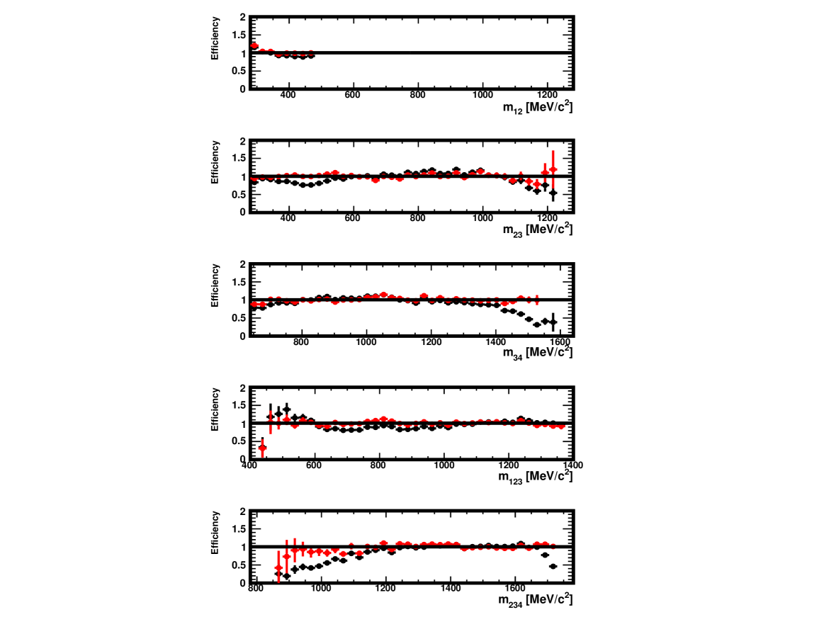
Figure 17: Efficiency in $m_{12}$, $m_{23}$, $m_{34}$, $m_{123}$ and $m_{234}$ in the data generated for this study, in the region $0<m_{12}<480$ MeV$/c^{2}$. Shown are the ratios of the distributions found in the distorted and original samples, with no correction (black) and for decays re-weighted using $\omega_{i}$ weights (red) as explained in Sect. 3.3. The absolute normalisation is arbitrary when the correction is not applied and natural when it is applied (red).

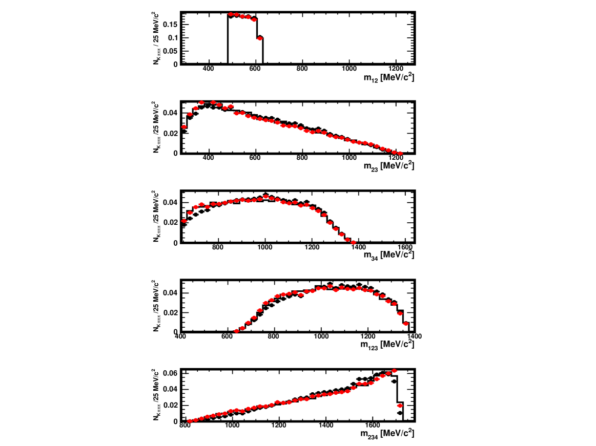
Figure 18: Distributions of $m_{12}$, $m_{23}$, $m_{34}$, $m_{123}$ and $m_{234}$ in the original sample (histogram), in the distorted one (full black circles) and in the distorted sample where the decays have been re-weighted using the $\omega_{i}$ weights (red), as explained in Sect. 3.3. The data used here are restricted to the region $480<m_{12}<620$ MeV$/c^{2}$. The absolute normalisation is arbitrary when the correction is not applied and natural when it is applied (red).

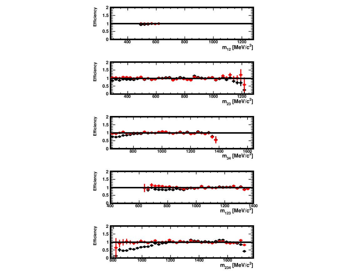
Figure 19: Efficiency in $m_{12}$, $m_{23}$, $m_{34}$, $m_{123}$ and $m_{234}$ in the data generated for this study, in the region $<480m_{12}<620$ MeV$/c^{2}$. Shown are the ratios of the distributions found in the distorted and original samples, with no correction (black) and for decays re-weighted using $\omega_{i}$ weights (red) as explained in Sect. 3.3. The absolute normalisation is arbitrary when the correction is not applied and natural when it is applied (red).

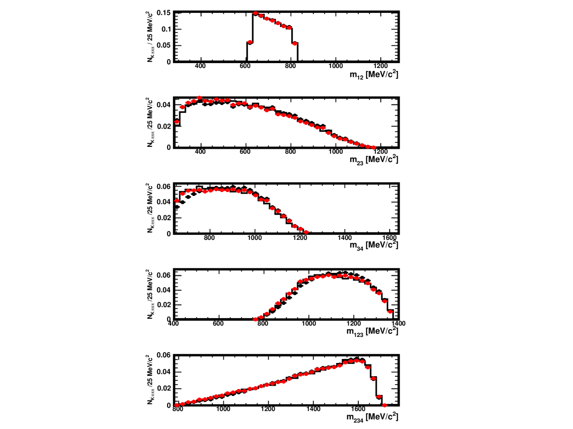
Figure 20: Distributions of $m_{12}$, $m_{23}$, $m_{34}$, $m_{123}$ and $m_{234}$ in the original sample (histogram), in the distorted one (full black circles) and in the distorted sample where the decays have been re-weighted using the $\omega_{i}$ weights (red), as explained in Sect. 3.3. The data used here are restricted to the region $620<m_{12}<820$ MeV$/c^{2}$. The absolute normalisation is arbitrary when the correction is not applied and natural when it is applied (red).

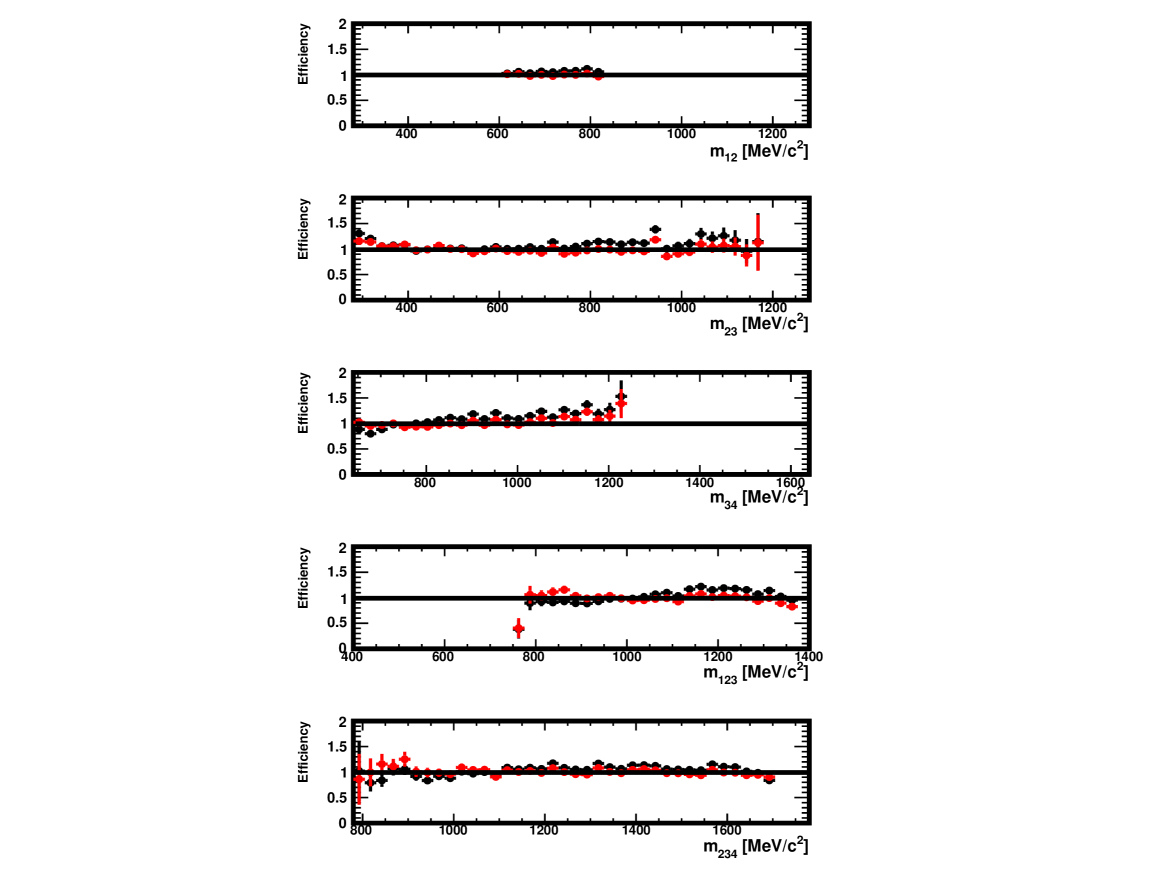
Figure 21: Efficiency in $m_{12}$, $m_{23}$, $m_{34}$, $m_{123}$ and $m_{234}$ in the data generated for this study, in the region $620<m_{12}<820$ MeV$/c^{2}$. Shown are the ratios of the distributions found in the distorted and original samples, with no correction (black) and for decays re-weighted using $\omega_{i}$ weights (red) as explained in Sect. 3.3. The absolute normalisation is arbitrary when the correction is not applied and natural when it is applied (red).

Figure 22: Distributions of $m_{12}$, $m_{23}$, $m_{34}$, $m_{123}$ and $m_{234}$ in the original sample (histogram), in the distorted one (full black circles) and in the distorted sample where the decays have been re-weighted using the $\omega_{i}$ weights (red), as explained in Sect. 3.3. The data used here are restricted to the region $820<m_{12}$ MeV$/c^{2}$. The absolute normalisation is arbitrary when the correction is not applied and natural when it is applied (red).

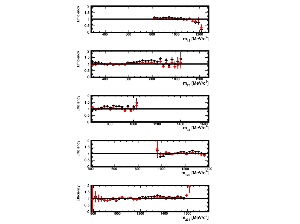
Figure 23: Efficiency in $m_{12}$, $m_{23}$, $m_{34}$, $m_{123}$ and $m_{234}$ in the data generated for this study, in the region $820<m_{12}$ MeV$/c^{2}$. Shown are the ratios of the distributions found in the distorted and original samples, with no correction (black) and for decays re-weighted using $\omega_{i}$ weights (red) as explained in Sect. 3.3. The absolute normalisation is arbitrary when the correction is not applied and natural when it is applied (red).

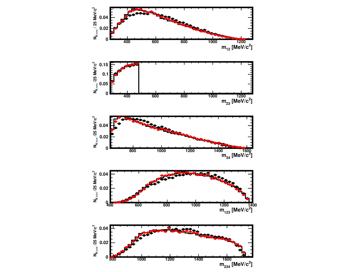
Figure 24: Distributions of $m_{12}$, $m_{23}$, $m_{34}$, $m_{123}$ and $m_{234}$ in the original sample (histogram), in the distorted one (full black circles) and in the distorted sample where the decays have been re-weighted using the $\omega_{i}$ weights (red), as explained in Sect. 3.3. The data used here are restricted to the region $0<m_{23}<480$ MeV$/c^{2}$. The absolute normalisation is arbitrary when the correction is not applied and natural when it is applied (red).

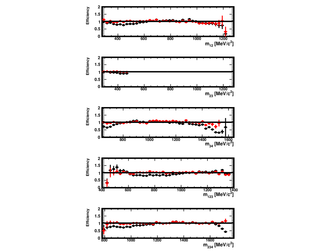
Figure 25: Efficiency in $m_{12}$, $m_{23}$, $m_{34}$, $m_{123}$ and $m_{234}$ in the data generated for this study, in the region $0<m_{23}<480$ MeV$/c^{2}$. Shown are the ratios of the distributions found in the distorted and original samples, with no correction (black) and for decays re-weighted using $\omega_{i}$ weights (red) as explained in Sect. 3.3. The absolute normalisation is arbitrary when the correction is not applied and natural when it is applied (red).

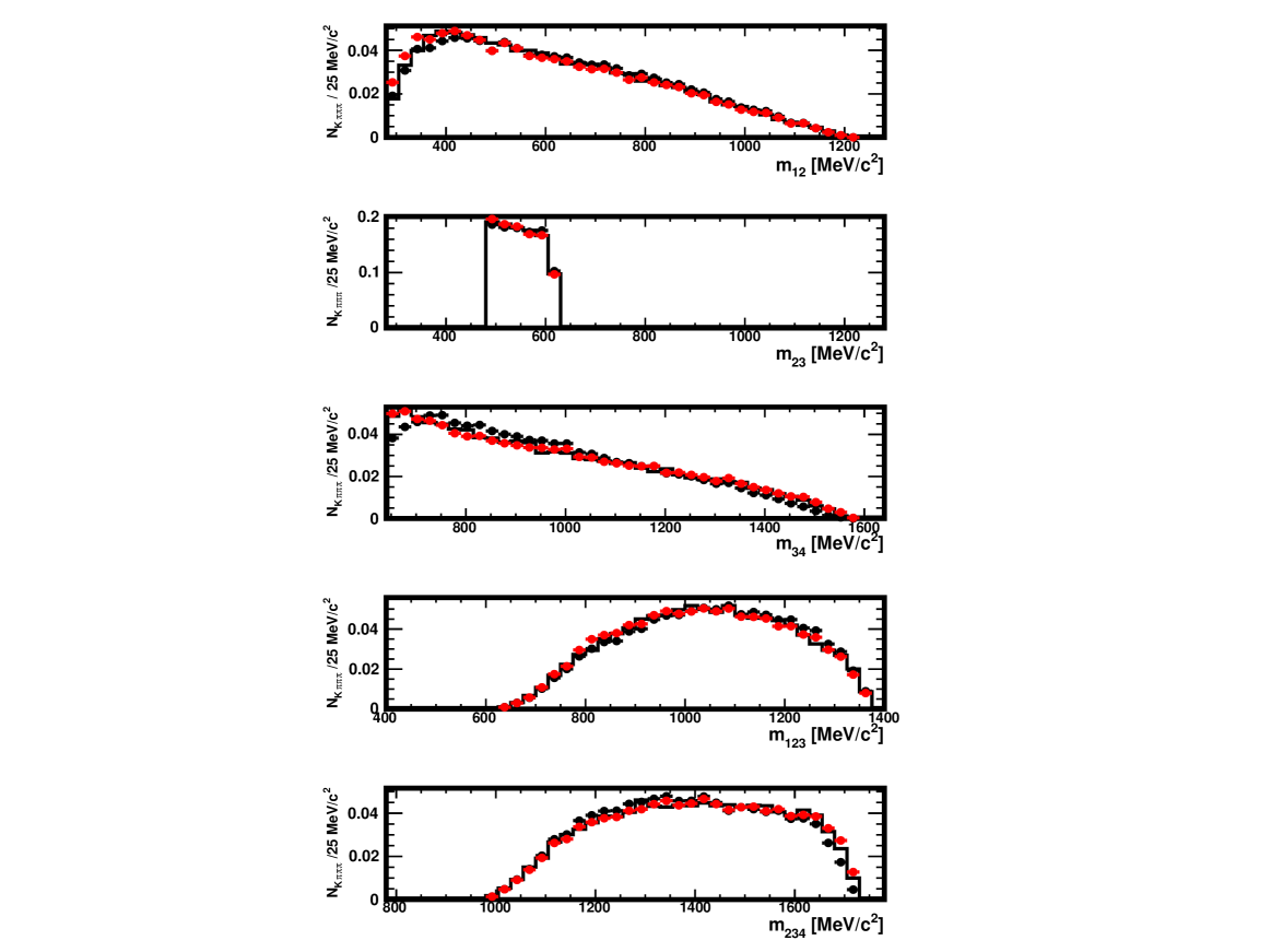
Figure 26: Distributions of $m_{12}$, $m_{23}$, $m_{34}$, $m_{123}$ and $m_{234}$ in the original sample (histogram), in the distorted one (full black circles) and in the distorted sample where the decays have been re-weighted using the $\omega_{i}$ weights (red), as explained in Sect. 3.3. The data used here are restricted to the region $480<m_{23}<620$ MeV$/c^{2}$. The absolute normalisation is arbitrary when the correction is not applied and natural when it is applied (red).

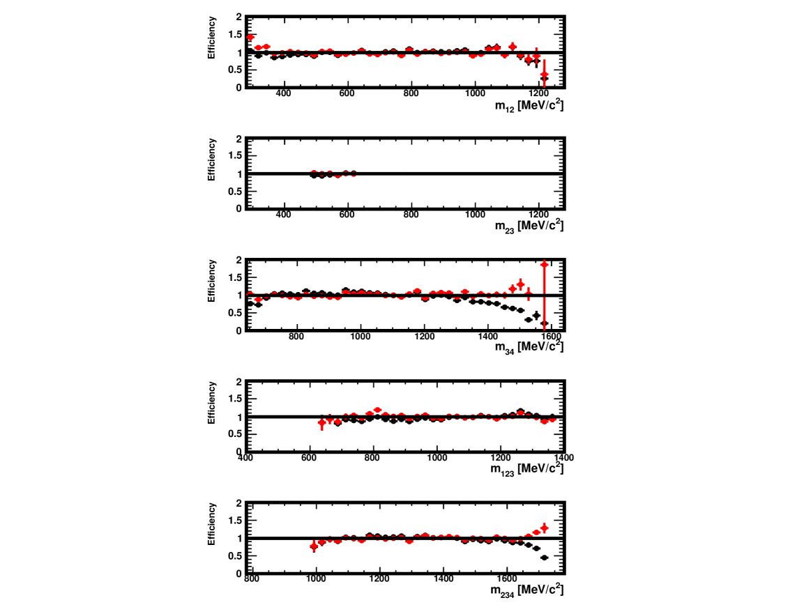
Figure 27: Efficiency in $m_{12}$, $m_{23}$, $m_{34}$, $m_{123}$ and $m_{234}$ in the data generated for this study, in the region $<480m_{23}<620$ MeV$/c^{2}$. Shown are the ratios of the distributions found in the distorted and original samples, with no correction (black) and for decays re-weighted using $\omega_{i}$ weights (red) as explained in Sect. 3.3. The absolute normalisation is arbitrary when the correction is not applied and natural when it is applied (red).

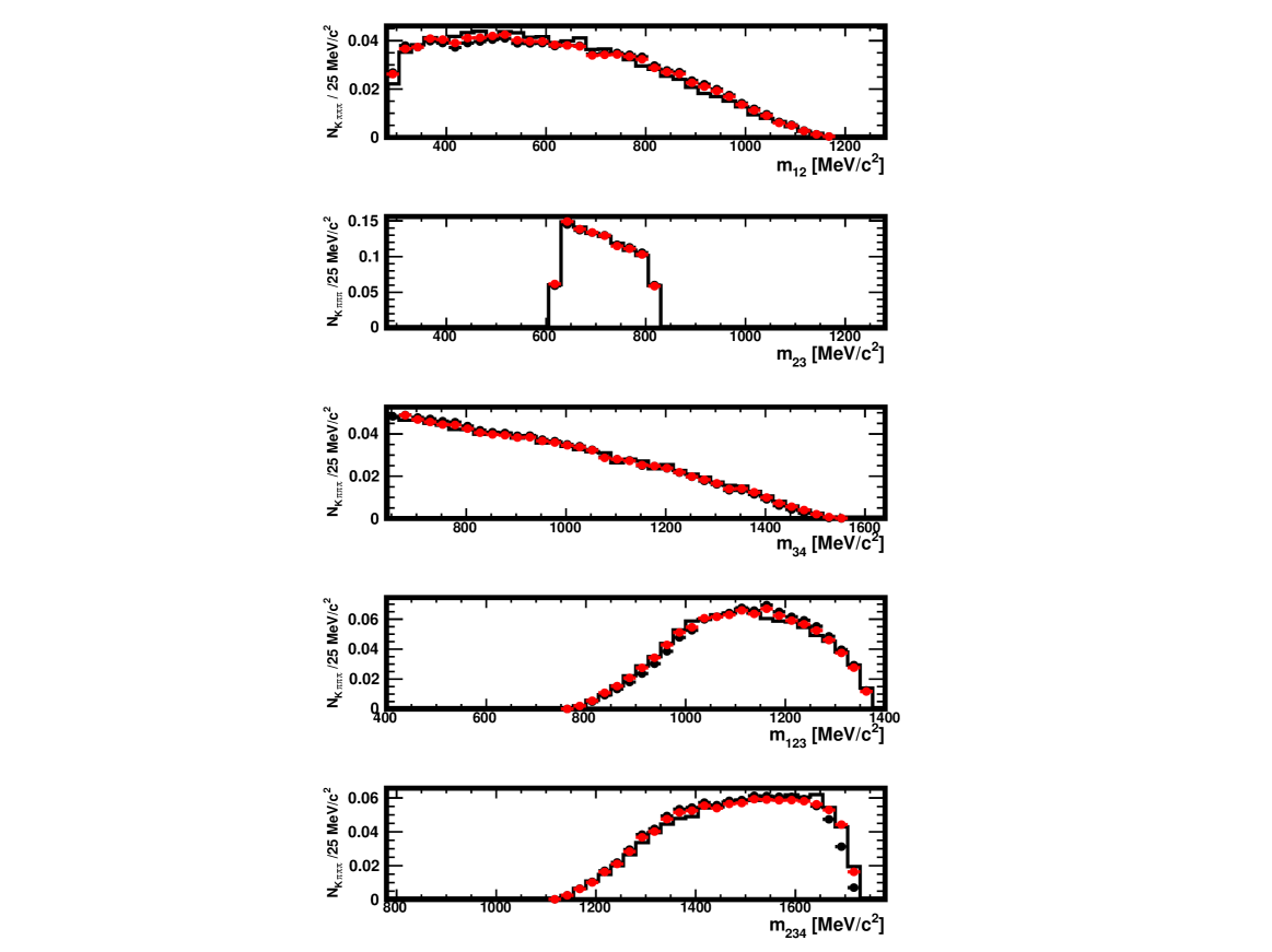
Figure 28: Distributions of $m_{12}$, $m_{23}$, $m_{34}$, $m_{123}$ and $m_{234}$ in the original sample (histogram), in the distorted one (full black circles) and in the distorted sample where the decays have been re-weighted using the $\omega_{i}$ weights (red), as explained in Sect. 3.3. The data used here are restricted to the region $620<m_{23}<820$ MeV$/c^{2}$. The absolute normalisation is arbitrary when the correction is not applied and natural when it is applied (red).

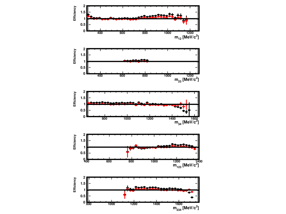
Figure 29: Efficiency in $m_{12}$, $m_{23}$, $m_{34}$, $m_{123}$ and $m_{234}$ in the data generated for this study, in the region $620<m_{23}<820$ MeV$/c^{2}$. Shown are the ratios of the distributions found in the distorted and original samples, with no correction (black) and for decays re-weighted using $\omega_{i}$ weights (red) as explained in Sect. 3.3. The absolute normalisation is arbitrary when the correction is not applied and natural when it is applied (red).

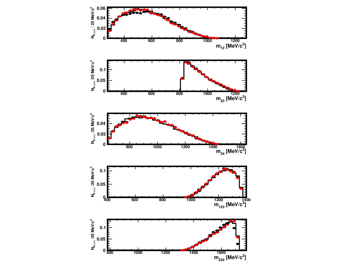
Figure 30: Distributions of $m_{12}$, $m_{23}$, $m_{34}$, $m_{123}$ and $m_{234}$ in the original sample (histogram), in the distorted one (full black circles) and in the distorted sample where the decays have been re-weighted using the $\omega_{i}$ weights (red), as explained in Sect. 3.3. The data used here are restricted to the region $820<m_{23}$ MeV$/c^{2}$. The absolute normalisation is arbitrary when the correction is not applied and natural when it is applied (red).

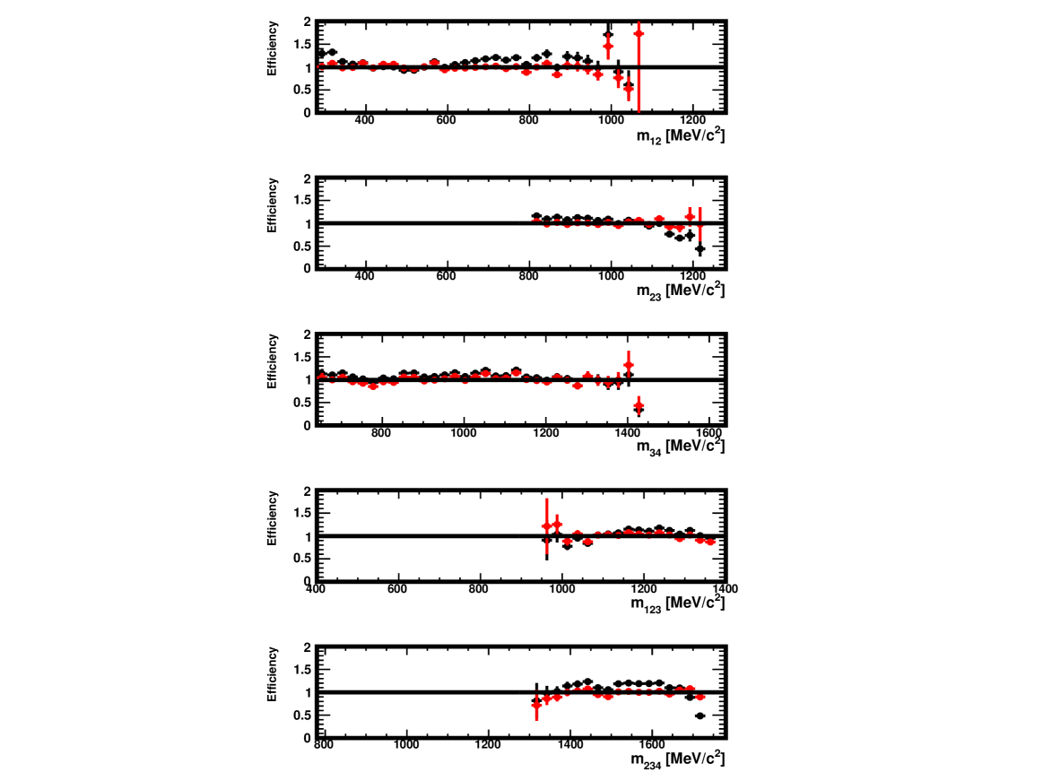
Figure 31: Efficiency in $m_{12}$, $m_{23}$, $m_{34}$, $m_{123}$ and $m_{234}$ in the data generated for this study, in the region $820<m_{23}$ MeV$/c^{2}$. Shown are the ratios of the distributions found in the distorted and original samples, with no correction (black) and for decays re-weighted using $\omega_{i}$ weights (red) as explained in Sect. 3.3. The absolute normalisation is arbitrary when the correction is not applied and natural when it is applied (red).

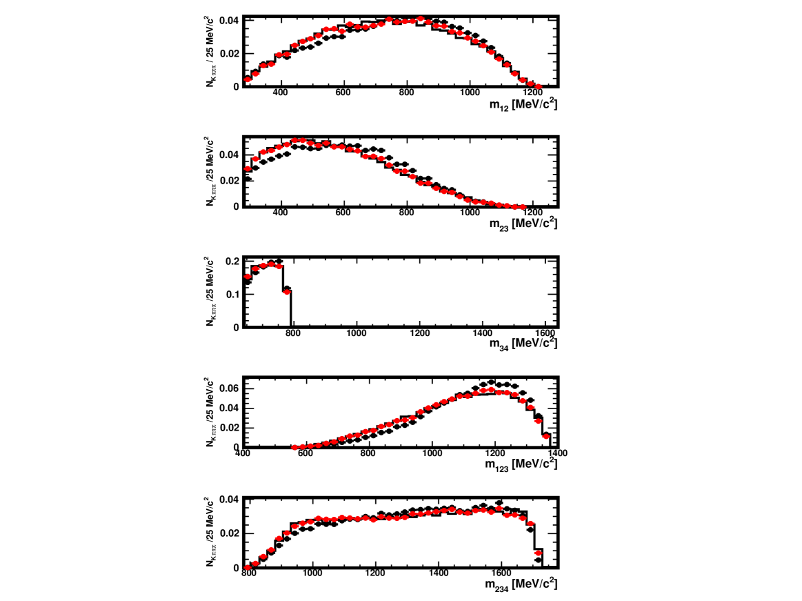
Figure 32: Distributions of $m_{12}$, $m_{23}$, $m_{34}$, $m_{123}$ and $m_{234}$ in the original sample (histogram), in the distorted one (full black circles) and in the distorted sample where the decays have been re-weighted using the $\omega_{i}$ weights (red), as explained in Sect. 3.3. The data used here are restricted to the region $0<m_{34}<780$ MeV$/c^{2}$. The absolute normalisation is arbitrary when the correction is not applied and natural when it is applied (red).

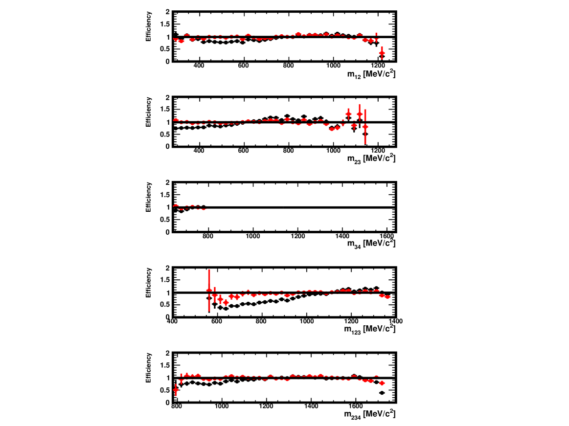
Figure 33: Efficiency in $m_{12}$, $m_{23}$, $m_{34}$, $m_{123}$ and $m_{234}$ in the data generated for this study, in the region $0<m_{34}<780$ MeV$/c^{2}$. Shown are the ratios of the distributions found in the distorted and original samples, with no correction (black) and for decays re-weighted using $\omega_{i}$ weights (red) as explained in Sect. 3.3. The absolute normalisation is arbitrary when the correction is not applied and natural when it is applied (red).

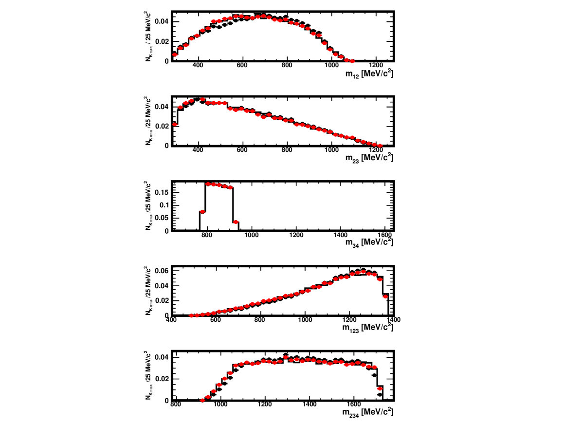
Figure 34: Distributions of $m_{12}$, $m_{23}$, $m_{34}$, $m_{123}$ and $m_{234}$ in the original sample (histogram), in the distorted one (full black circles) and in the distorted sample where the decays have been re-weighted using the $\omega_{i}$ weights (red), as explained in Sect. 3.3. The data used here are restricted to the region $780<m_{34}<920$ MeV$/c^{2}$. The absolute normalisation is arbitrary when the correction is not applied and natural when it is applied (red).

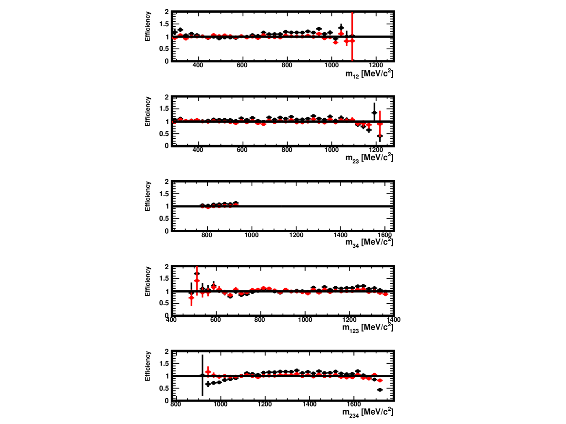
Figure 35: Efficiency in $m_{12}$, $m_{23}$, $m_{34}$, $m_{123}$ and $m_{234}$ in the data generated for this study, in the region $<780m_{34}<920$ MeV$/c^{2}$. Shown are the ratios of the distributions found in the distorted and original samples, with no correction (black) and for decays re-weighted using $\omega_{i}$ weights (red) as explained in Sect. 3.3. The absolute normalisation is arbitrary when the correction is not applied and natural when it is applied (red).

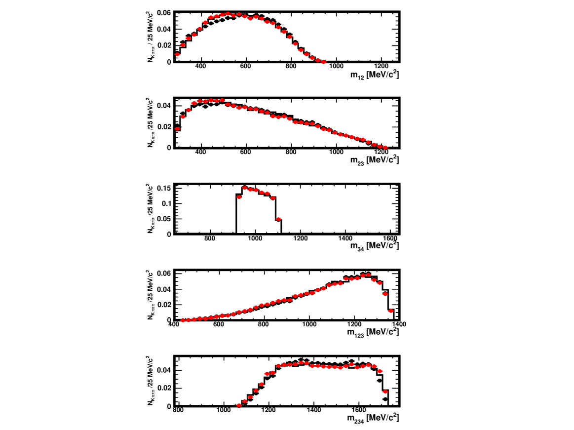
Figure 36: Distributions of $m_{12}$, $m_{23}$, $m_{34}$, $m_{123}$ and $m_{234}$ in the original sample (histogram), in the distorted one (full black circles) and in the distorted sample where the decays have been re-weighted using the $\omega_{i}$ weights (red), as explained in Sect. 3.3. The data used here are restricted to the region $920<m_{34}<1100$ MeV$/c^{2}$. The absolute normalisation is arbitrary when the correction is not applied and natural when it is applied (red).

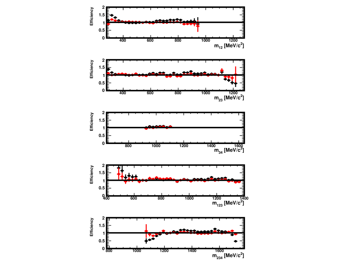
Figure 37: Efficiency in $m_{12}$, $m_{23}$, $m_{34}$, $m_{123}$ and $m_{234}$ in the data generated for this study, in the region $920<m_{34}<1100$ MeV$/c^{2}$. Shown are the ratios of the distributions found in the distorted and original samples, with no correction (black) and for decays re-weighted using $\omega_{i}$ weights (red) as explained in Sect. 3.3. The absolute normalisation is arbitrary when the correction is not applied and natural when it is applied (red).

Figure 38: Distributions of $m_{12}$, $m_{23}$, $m_{34}$, $m_{123}$ and $m_{234}$ in the original sample (histogram), in the distorted one (full black circles) and in the distorted sample where the decays have been re-weighted using the $\omega_{i}$ weights (red), as explained in Sect. 3.3. The data used here are restricted to the region $1100<m_{34}$ MeV$/c^{2}$. The absolute normalisation is arbitrary when the correction is not applied and natural when it is applied (red).

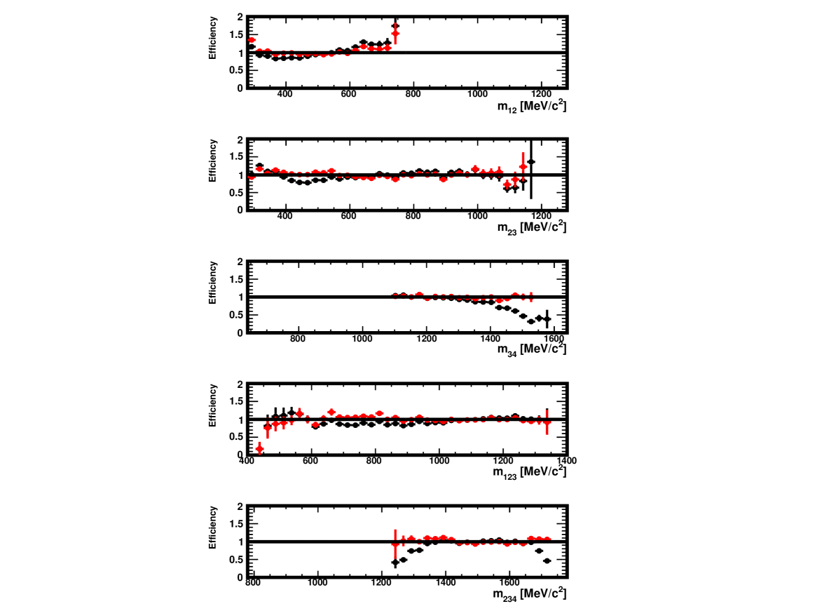
Figure 39: Efficiency in $m_{12}$, $m_{23}$, $m_{34}$, $m_{123}$ and $m_{234}$ in the data generated for this study, in the region $1100<m_{34}$ MeV$/c^{2}$. Shown are the ratios of the distributions found in the distorted and original samples, with no correction (black) and for decays re-weighted using $\omega_{i}$ weights (red) as explained in Sect. 3.3. The absolute normalisation is arbitrary when the correction is not applied and natural when it is applied (red).

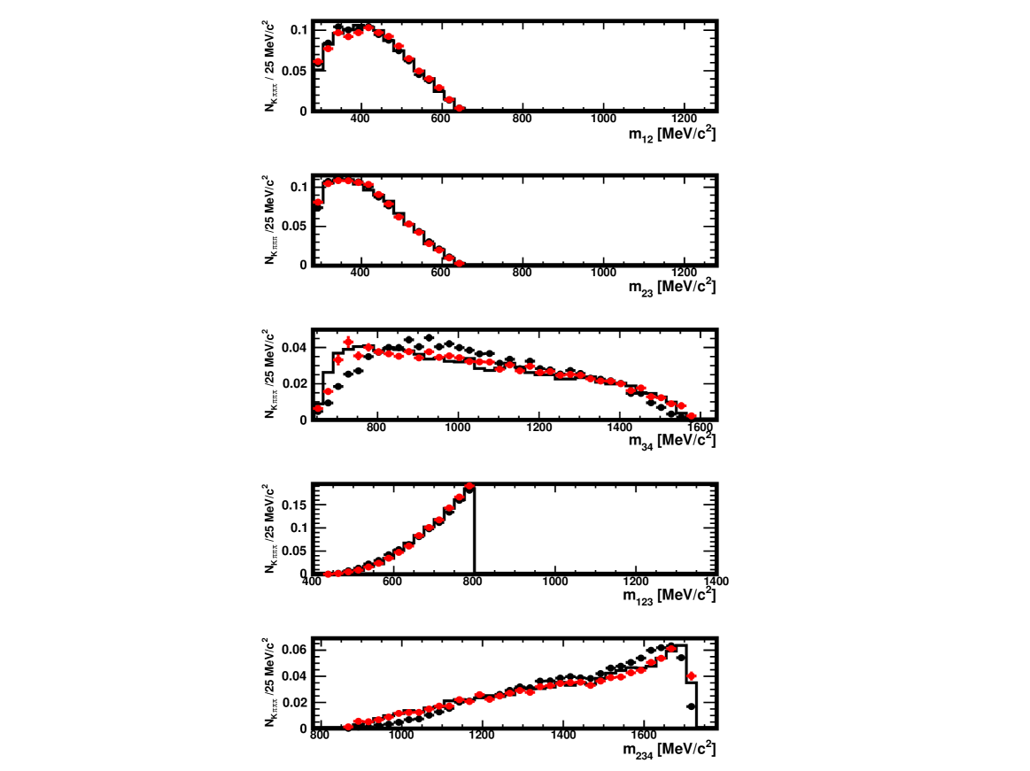
Figure 40: Distributions of $m_{12}$, $m_{23}$, $m_{34}$, $m_{123}$ and $m_{234}$ in the original sample (histogram), in the distorted one (full black circles) and in the distorted sample where the decays have been re-weighted using the $\omega_{i}$ weights (red), as explained in Sect. 3.3. The data used here are restricted to the region $0<m_{123}<800$ MeV$/c^{2}$. The absolute normalisation is arbitrary when the correction is not applied and natural when it is applied (red).

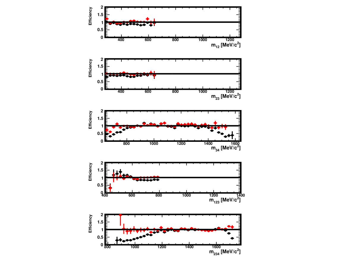
Figure 41: Efficiency in $m_{12}$, $m_{23}$, $m_{34}$, $m_{123}$ and $m_{234}$ in the data generated for this study, in the region $0<m_{123}<800$ MeV$/c^{2}$. Shown are the ratios of the distributions found in the distorted and original samples, with no correction (black) and for decays re-weighted using $\omega_{i}$ weights (red) as explained in Sect. 3.3. The absolute normalisation is arbitrary when the correction is not applied and natural when it is applied (red).

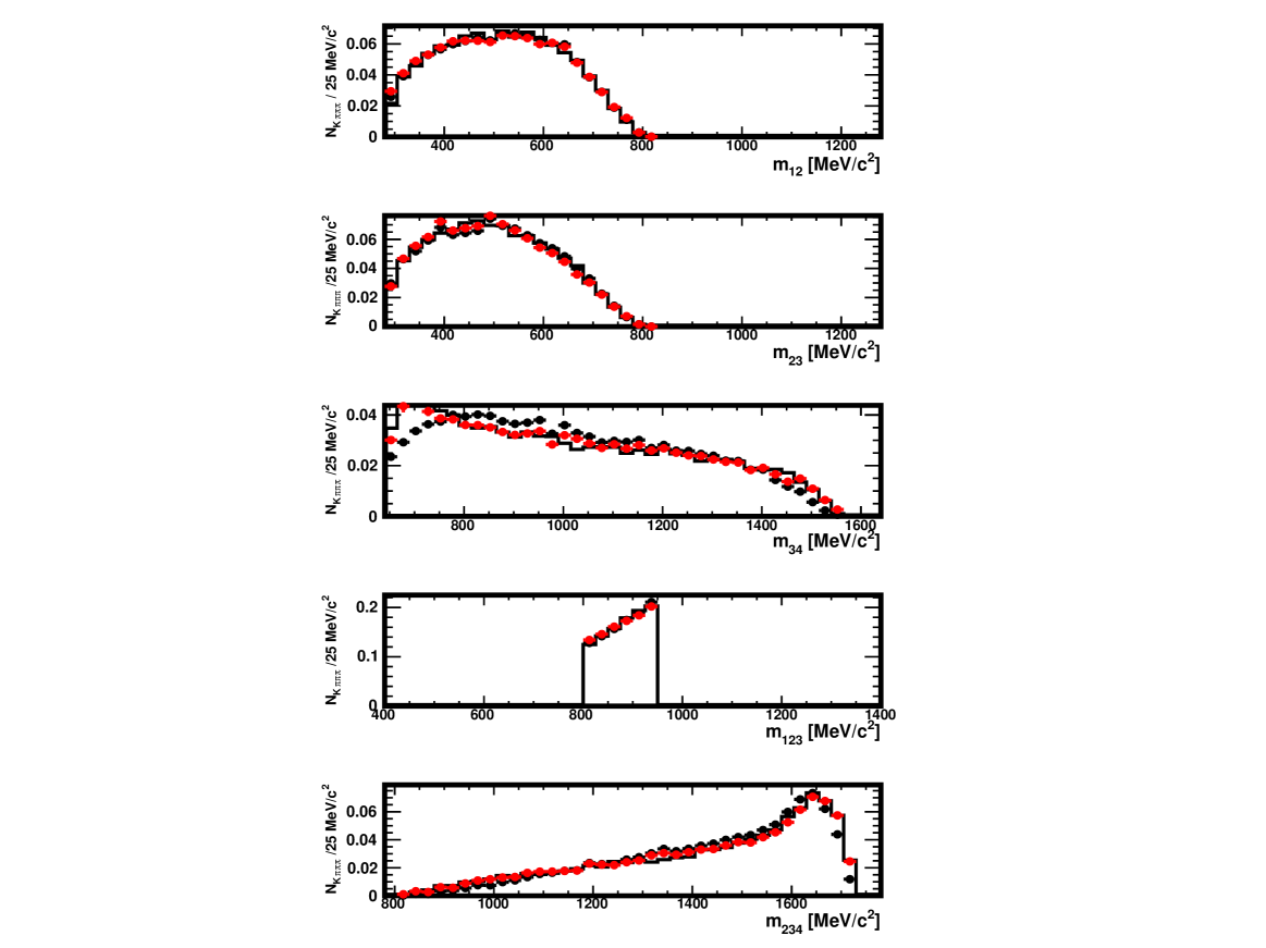
Figure 42: Distributions of $m_{12}$, $m_{23}$, $m_{123}$, $m_{123}$ and $m_{234}$ in the original sample (histogram), in the distorted one (full black circles) and in the distorted sample where the decays have been re-weighted using the $\omega_{i}$ weights (red), as explained in Sect. 3.3. The data used here are restricted to the region $800<m_{123}<950$ MeV$/c^{2}$. The absolute normalisation is arbitrary when the correction is not applied and natural when it is applied (red).

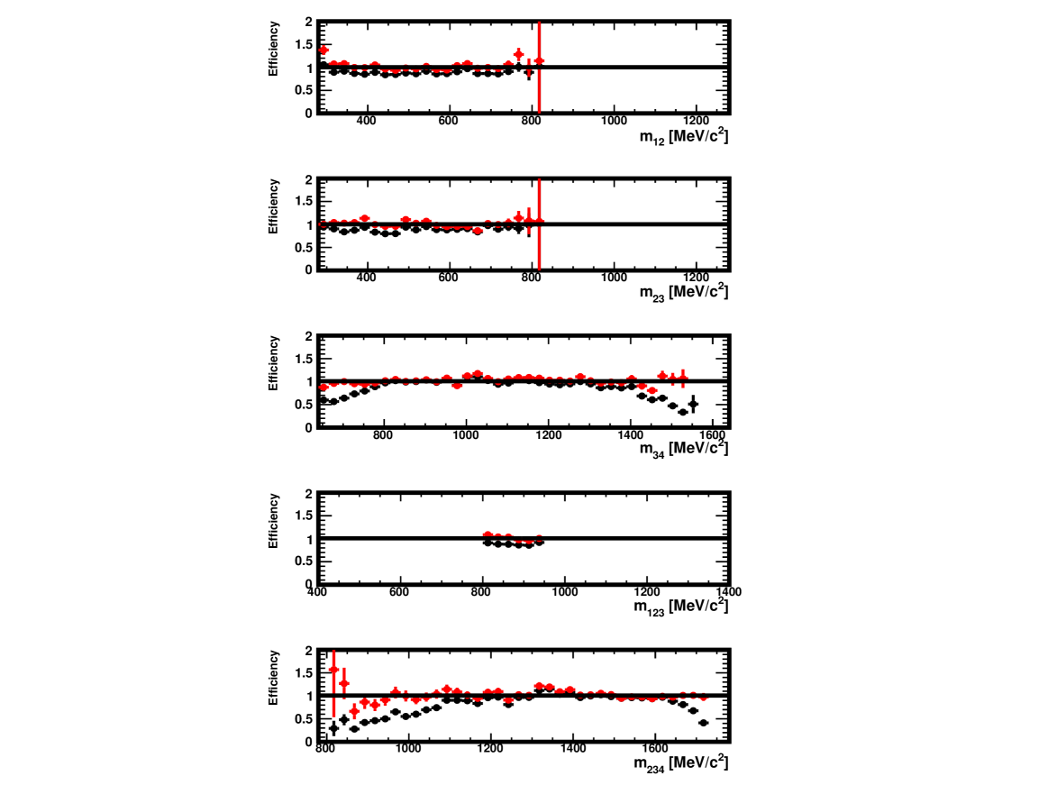
Figure 43: Efficiency in $m_{12}$, $m_{23}$, $m_{34}$, $m_{123}$ and $m_{234}$ in the data generated for this study, in the region $<800m_{123}<950$ MeV$/c^{2}$. Shown are the ratios of the distributions found in the distorted and original samples, with no correction (black) and for decays re-weighted using $\omega_{i}$ weights (red) as explained in Sect. 3.3. The absolute normalisation is arbitrary when the correction is not applied and natural when it is applied (red).

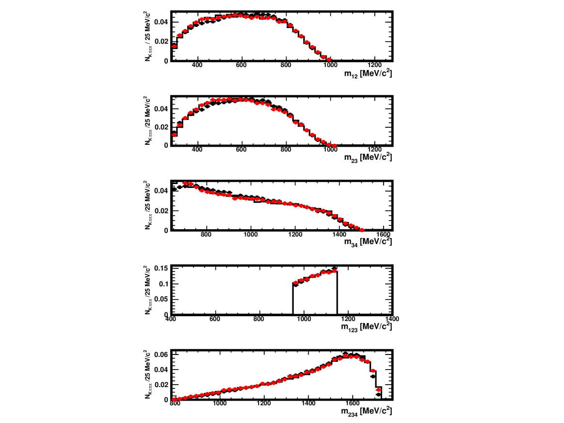
Figure 44: Distributions of $m_{12}$, $m_{23}$, $m_{34}$, $m_{123}$ and $m_{234}$ in the original sample (histogram), in the distorted one (full black circles) and in the distorted sample where the decays have been re-weighted using the $\omega_{i}$ weights (red), as explained in Sect. 3.3. The data used here are restricted to the region $950<m_{123}<1150$ MeV$/c^{2}$. The absolute normalisation is arbitrary when the correction is not applied and natural when it is applied (red).

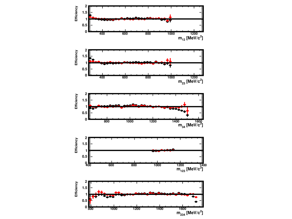
Figure 45: Efficiency in $m_{12}$, $m_{23}$, $m_{34}$, $m_{123}$ and $m_{234}$ in the data generated for this study, in the region $950<m_{123}<1150$ MeV$/c^{2}$. Shown are the ratios of the distributions found in the distorted and original samples, with no correction (black) and for decays re-weighted using $\omega_{i}$ weights (red) as explained in Sect. 3.3. The absolute normalisation is arbitrary when the correction is not applied and natural when it is applied (red).

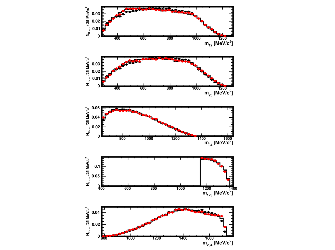
Figure 46: Distributions of $m_{12}$, $m_{23}$, $m_{34}$, $m_{123}$ and $m_{234}$ in the original sample (histogram), in the distorted one (full black circles) and in the distorted sample where the decays have been re-weighted using the $\omega_{i}$ weights (red), as explained in Sect. 3.3. The data used here are restricted to the region $1150<m_{123}$ MeV$/c^{2}$. The absolute normalisation is arbitrary when the correction is not applied and natural when it is applied (red).

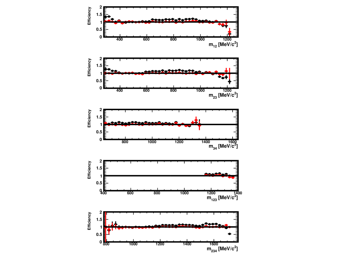
Figure 47: Efficiency in $m_{12}$, $m_{23}$, $m_{34}$, $m_{123}$ and $m_{234}$ in the data generated for this study, in the region $1150<m_{123}$ MeV$/c^{2}$. Shown are the ratios of the distributions found in the distorted and original samples, with no correction (black) and for decays re-weighted using $\omega_{i}$ weights (red) as explained in Sect. 3.3. The absolute normalisation is arbitrary when the correction is not applied and natural when it is applied (red).

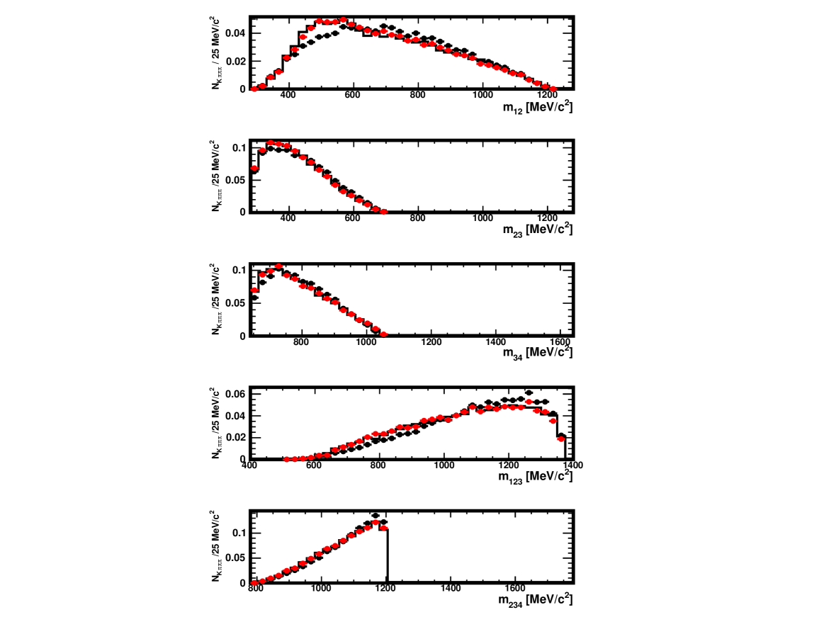
Figure 48: Distributions of $m_{12}$, $m_{23}$, $m_{34}$, $m_{123}$ and $m_{234}$ in the original sample (histogram), in the distorted one (full black circles) and in the distorted sample where the decays have been re-weighted using the $\omega_{i}$ weights (red), as explained in Sect. 3.3. The data used here are restricted to the region $0<m_{234}<800$ MeV$/c^{2}$. The absolute normalisation is arbitrary when the correction is not applied and natural when it is applied (red).

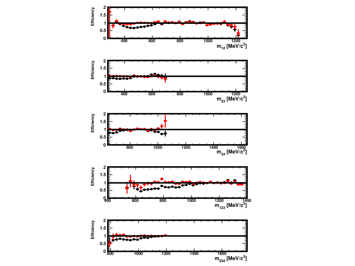
Figure 49: Efficiency in $m_{12}$, $m_{23}$, $m_{34}$, $m_{123}$ and $m_{234}$ in the data generated for this study, in the region $0<m_{234}<800$ MeV$/c^{2}$. Shown are the ratios of the distributions found in the distorted and original samples, with no correction (black) and for decays re-weighted using $\omega_{i}$ weights (red) as explained in Sect. 3.3. The absolute normalisation is arbitrary when the correction is not applied and natural when it is applied (red).

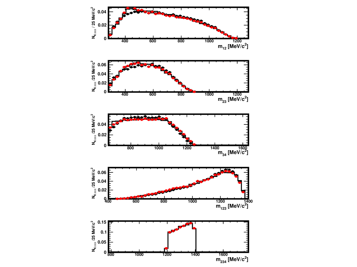
Figure 50: Distributions of $m_{12}$, $m_{23}$, $m_{123}$, $m_{123}$ and $m_{234}$ in the original sample (histogram), in the distorted one (full black circles) and in the distorted sample where the decays have been re-weighted using the $\omega_{i}$ weights (red), as explained in Sect. 3.3. The data used here are restricted to the region $800<m_{234}<950$ MeV$/c^{2}$. The absolute normalisation is arbitrary when the correction is not applied and natural when it is applied (red).

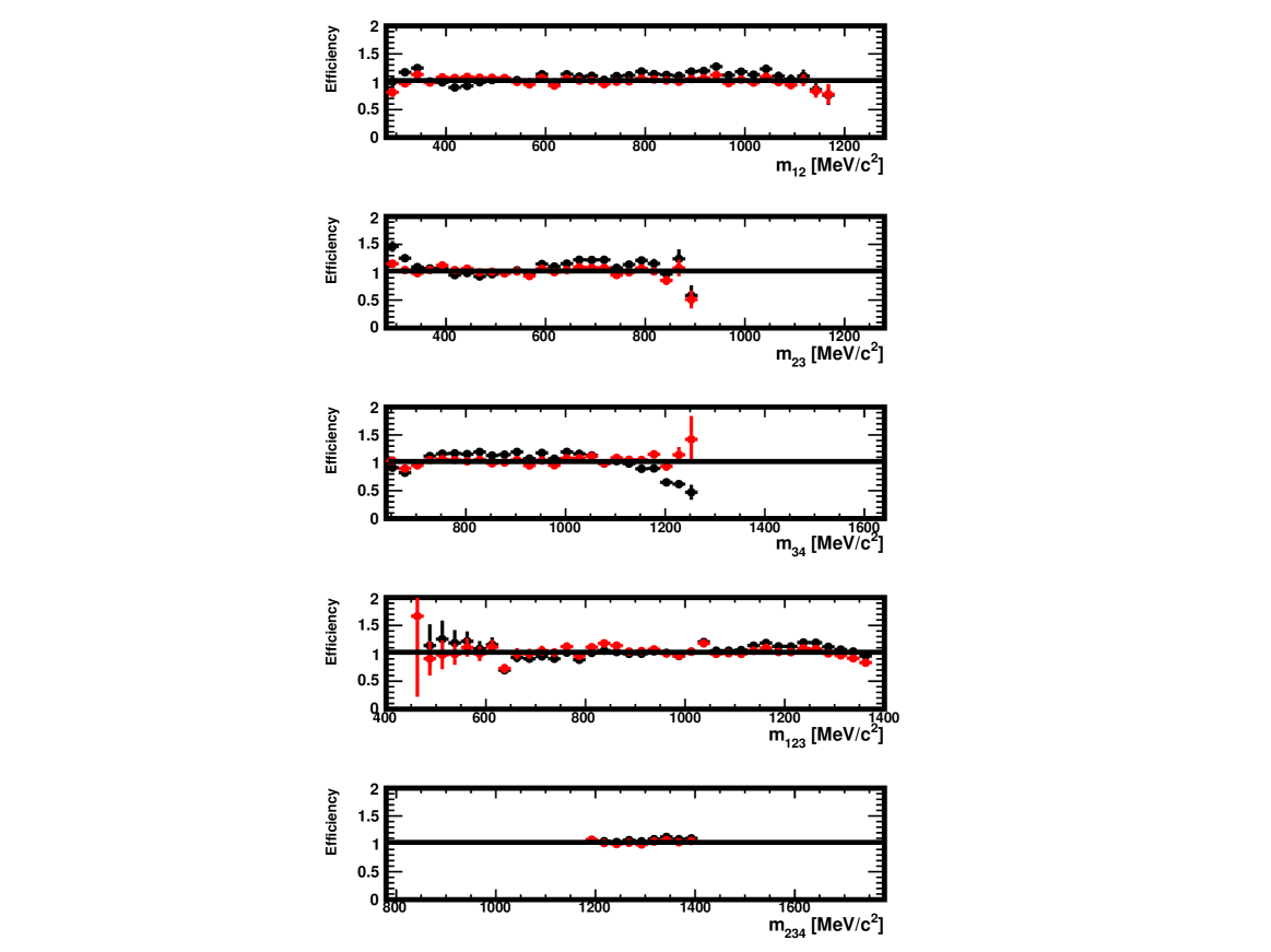
Figure 51: Efficiency in $m_{12}$, $m_{23}$, $m_{34}$, $m_{123}$ and $m_{234}$ in the data generated for this study, in the region $<800m_{234}<950$ MeV$/c^{2}$. Shown are the ratios of the distributions found in the distorted and original samples, with no correction (black) and for decays re-weighted using $\omega_{i}$ weights (red) as explained in Sect. 3.3. The absolute normalisation is arbitrary when the correction is not applied and natural when it is applied (red).

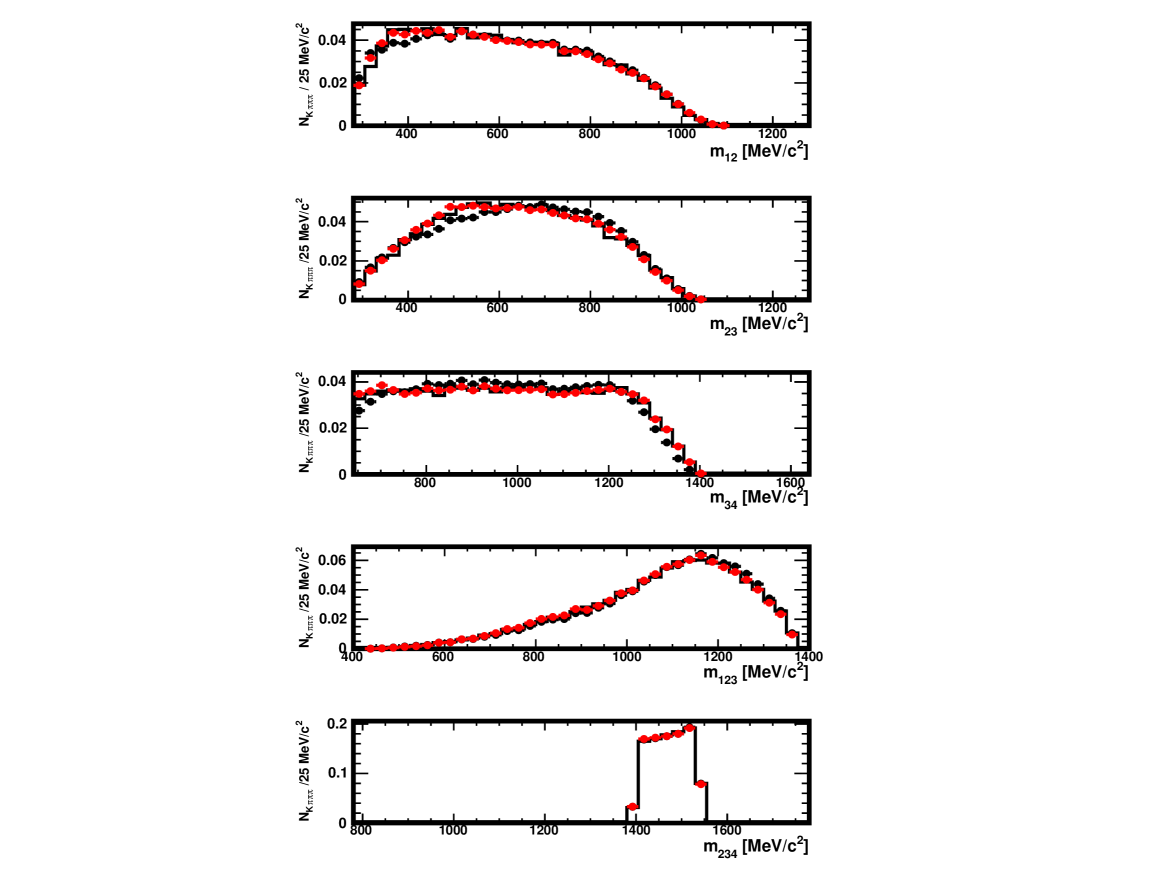
Figure 52: Distributions of $m_{12}$, $m_{23}$, $m_{34}$, $m_{123}$ and $m_{234}$ in the original sample (histogram), in the distorted one (full black circles) and in the distorted sample where the decays have been re-weighted using the $\omega_{i}$ weights (red), as explained in Sect. 3.3. The data used here are restricted to the region $950<m_{234}<1150$ MeV$/c^{2}$. The absolute normalisation is arbitrary when the correction is not applied and natural when it is applied (red).

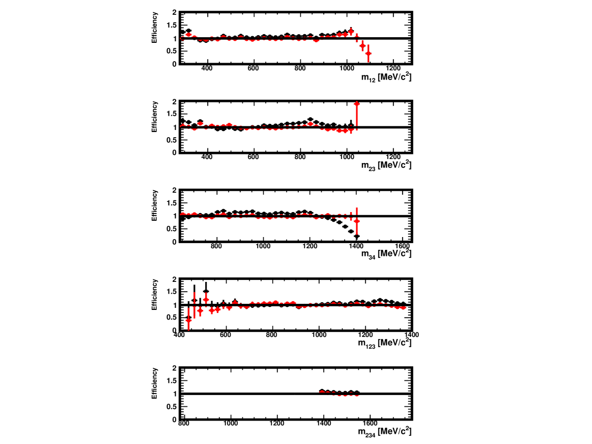
Figure 53: Efficiency in $m_{12}$, $m_{23}$, $m_{34}$, $m_{123}$ and $m_{234}$ in the data generated for this study, in the region $950<m_{234}<1150$ MeV$/c^{2}$. Shown are the ratios of the distributions found in the distorted and original samples, with no correction (black) and for decays re-weighted using $\omega_{i}$ weights (red) as explained in Sect. 3.3. The absolute normalisation is arbitrary when the correction is not applied and natural when it is applied (red).

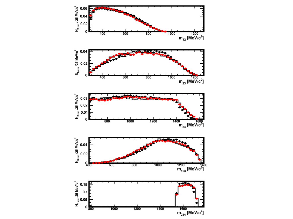
Figure 54: Distributions of $m_{12}$, $m_{23}$, $m_{34}$, $m_{123}$ and $m_{234}$ in the original sample (histogram), in the distorted one (full black circles) and in the distorted sample where the decays have been re-weighted using the $\omega_{i}$ weights (red), as explained in Sect. 3.3. The data used here are restricted to the region $1150<m_{234}$ MeV$/c^{2}$. The absolute normalisation is arbitrary when the correction is not applied and natural when it is applied (red).

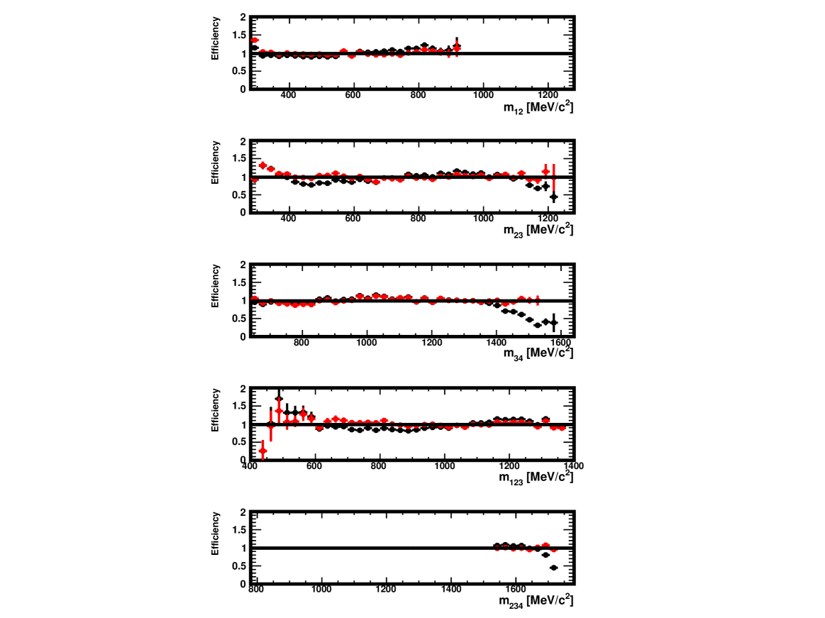
Figure 55: Efficiency in $m_{12}$, $m_{23}$, $m_{34}$, $m_{123}$ and $m_{234}$ in the data generated for this study, in the region $1150<m_{234}$ MeV$/c^{2}$. Shown are the ratios of the distributions found in the distorted and original samples, with no correction (black) and for decays re-weighted using $\omega_{i}$ weights (red) as explained in Sect. 3.3. The absolute normalisation is arbitrary when the correction is not applied and natural when it is applied (red).

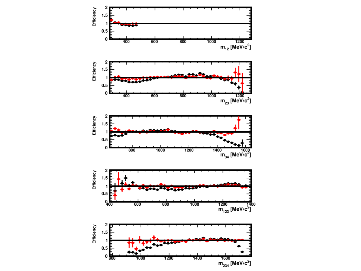
Figure 57: Efficiency in $m_{12}$, $m_{23}$, $m_{34}$, $m_{123}$ and $m_{234}$ in the data generated for this study, in the region $0<m_{12}<480$ MeV$/c^{2}$ and with a tighter selection. Shown are the ratios of the distributions found in the distorted and original samples, with no correction (black) and for decays re-weighted using $\omega_{i}$ weights (red) as explained in Sect. 3.3. The absolute normalisation is arbitrary when the correction is not applied and natural when it is applied (red).

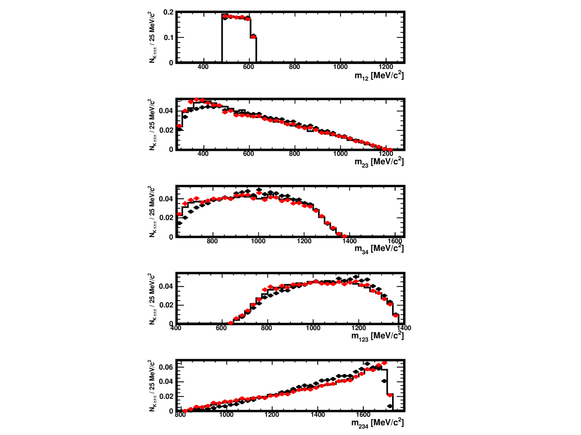
Figure 58: Distributions of $m_{12}$, $m_{23}$, $m_{34}$, $m_{123}$ and $m_{234}$ in the original sample (histogram), in the distorted one obtained with a tighter selection (full black circles) and in the distorted sample where the decays have been re-weighted using the $\omega_{i}$ weights (red), as explained in Sect. 3.3. The data used here are restricted to the region $480<m_{12}<620$ MeV$/c^{2}$. The absolute normalisation is arbitrary when the correction is not applied and natural when it is applied (red).

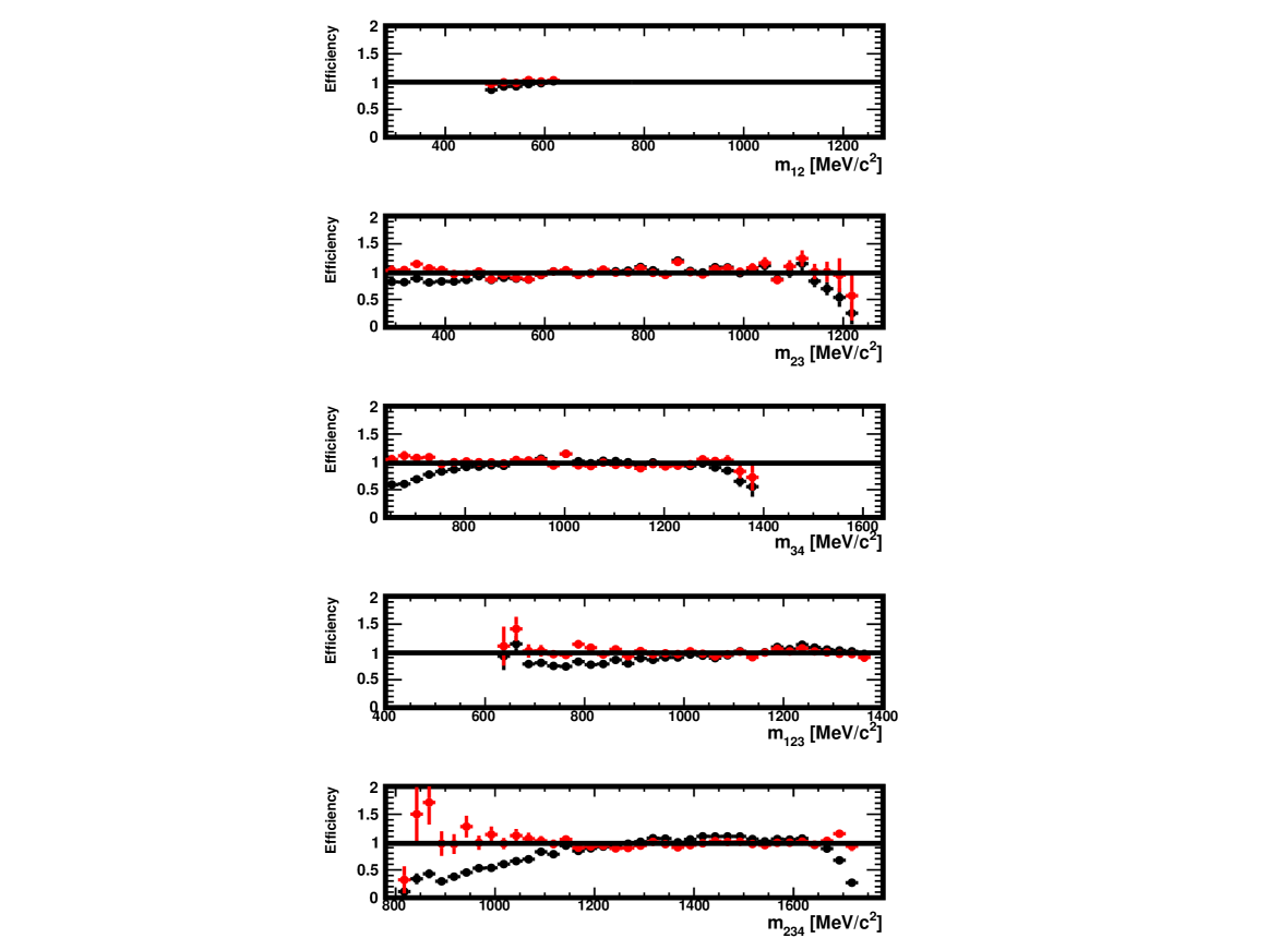
Figure 59: Efficiency in $m_{12}$, $m_{23}$, $m_{34}$, $m_{123}$ and $m_{234}$ in the data generated for this study, in the region $<480m_{12}<620$ MeV$/c^{2}$ and with a tighter selection. Shown are the ratios of the distributions found in the distorted and original samples, with no correction (black) and for decays re-weighted using $\omega_{i}$ weights (red) as explained in Sect. 3.3. The absolute normalisation is arbitrary when the correction is not applied and natural when it is applied (red).

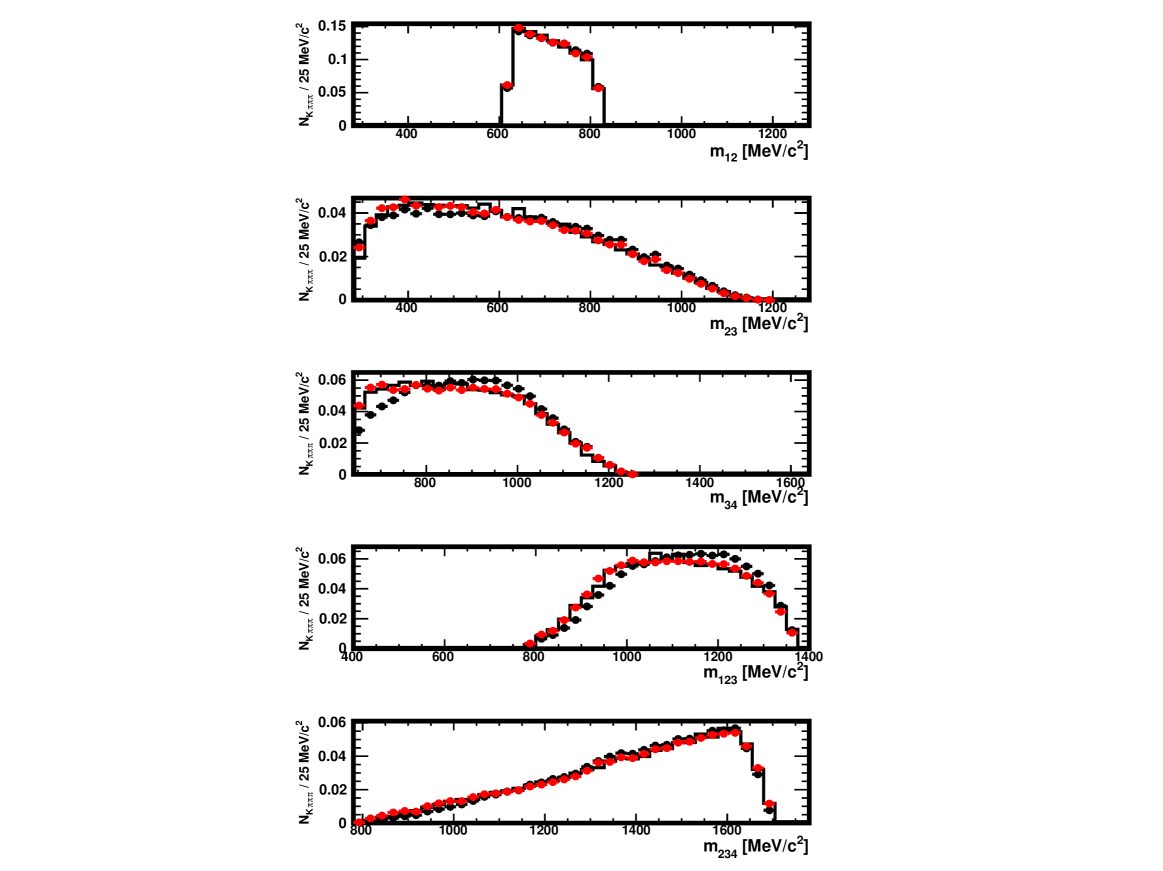
Figure 60: Distributions of $m_{12}$, $m_{23}$, $m_{34}$, $m_{123}$ and $m_{234}$ in the original sample (histogram), in the distorted one obtained with a tighter selection (full black circles) and in the distorted sample where the decays have been re-weighted using the $\omega_{i}$ weights (red), as explained in Sect. 3.3. The data used here are restricted to the region $620<m_{12}<820$ MeV$/c^{2}$. The absolute normalisation is arbitrary when the correction is not applied and natural when it is applied (red).

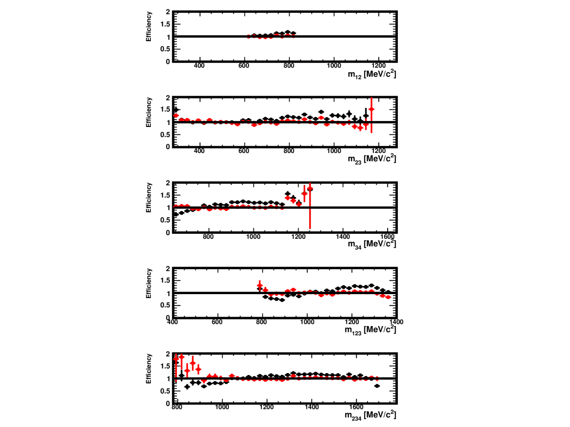
Figure 61: Efficiency in $m_{12}$, $m_{23}$, $m_{34}$, $m_{123}$ and $m_{234}$ in the data generated for this study, in the region $620<m_{12}<820$ MeV$/c^{2}$ and with a tighter selection. Shown are the ratios of the distributions found in the distorted and original samples, with no correction (black) and for decays re-weighted using $\omega_{i}$ weights (red) as explained in Sect. 3.3. The absolute normalisation is arbitrary when the correction is not applied and natural when it is applied (red).

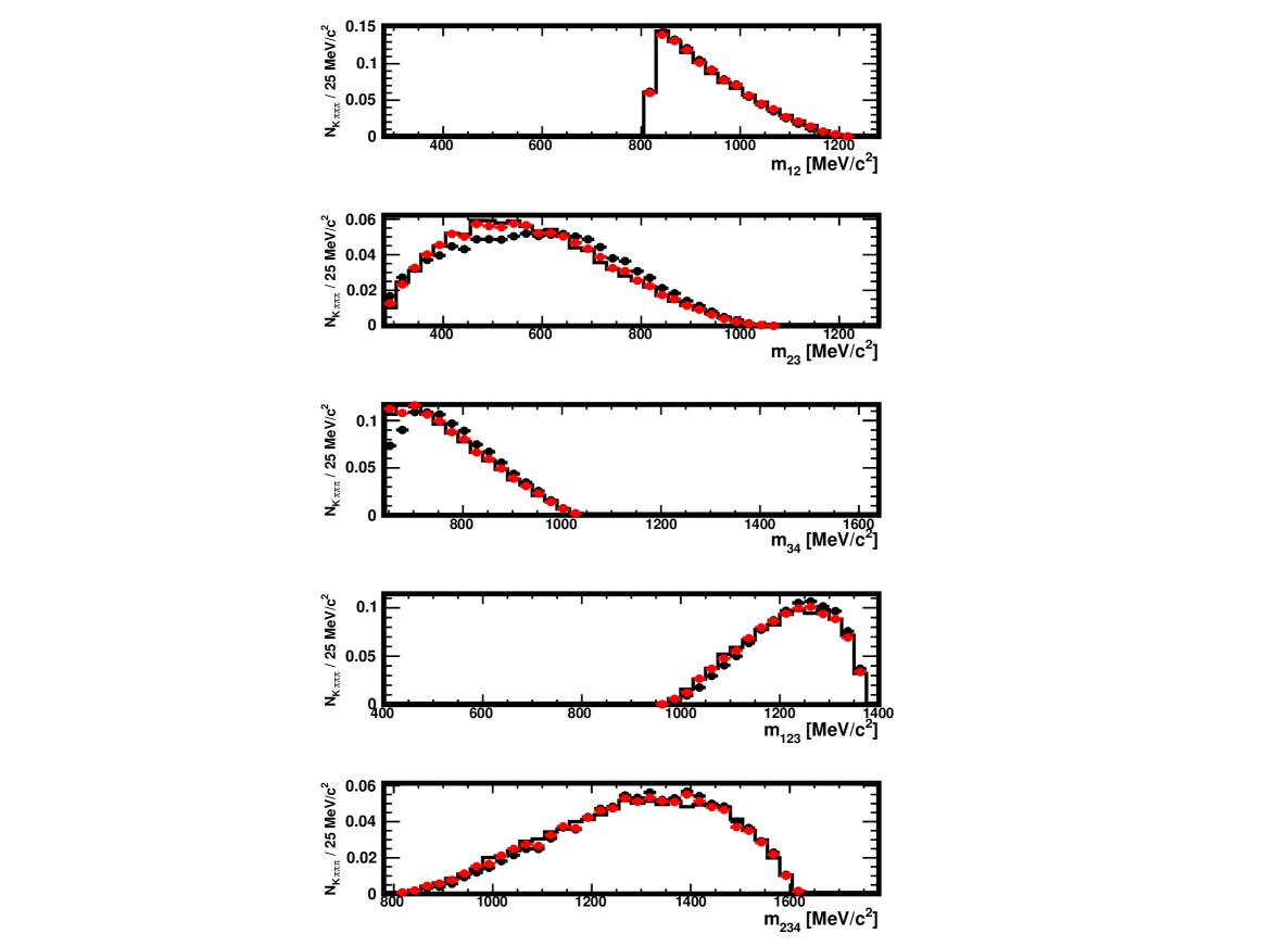
Figure 62: Distributions of $m_{12}$, $m_{23}$, $m_{34}$, $m_{123}$ and $m_{234}$ in the original sample (histogram), in the distorted one obtained with a tighter selection (full black circles) and in the distorted sample where the decays have been re-weighted using the $\omega_{i}$ weights (red), as explained in Sect. 3.3. The data used here are restricted to the region $820<m_{12}$ MeV$/c^{2}$. The absolute normalisation is arbitrary when the correction is not applied and natural when it is applied (red).

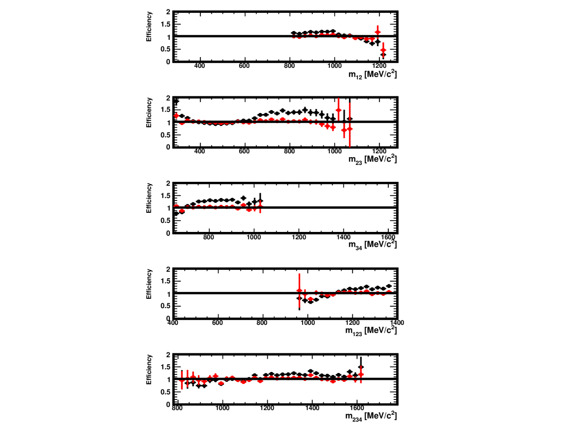
Figure 63: Efficiency in $m_{12}$, $m_{23}$, $m_{34}$, $m_{123}$ and $m_{234}$ in the data generated for this study, in the region $820<m_{12}$ MeV$/c^{2}$ and with a tighter selection. Shown are the ratios of the distributions found in the distorted and original samples, with no correction (black) and for decays re-weighted using $\omega_{i}$ weights (red) as explained in Sect. 3.3. The absolute normalisation is arbitrary when the correction is not applied and natural when it is applied (red).

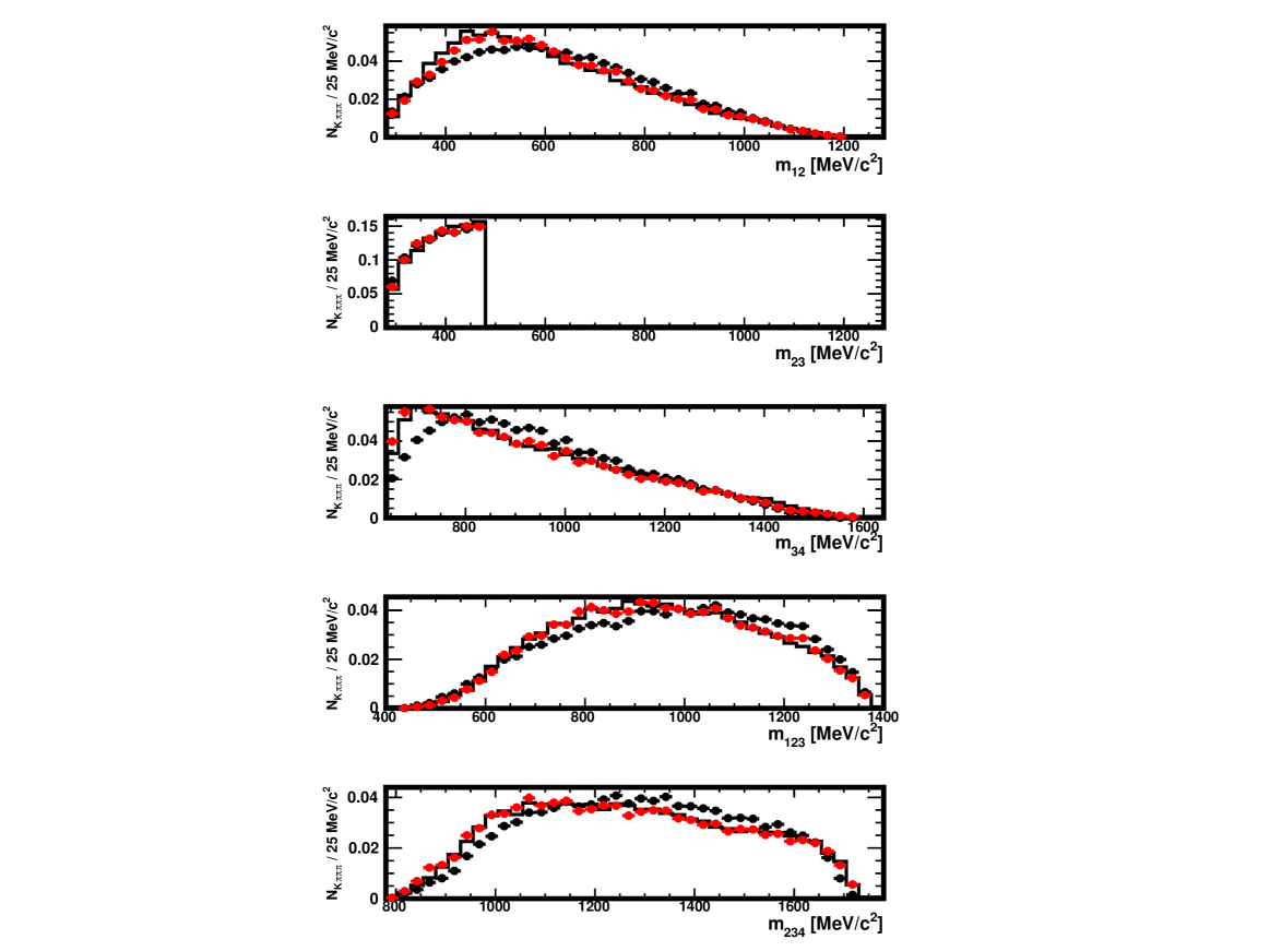
Figure 64: Distributions of $m_{12}$, $m_{23}$, $m_{34}$, $m_{123}$ and $m_{234}$ in the original sample (histogram), in the distorted one obtained with a tighter selection (full black circles) and in the distorted sample where the decays have been re-weighted using the $\omega_{i}$ weights (red), as explained in Sect. 3.3. The data used here are restricted to the region $0<m_{23}<480$ MeV$/c^{2}$. The absolute normalisation is arbitrary when the correction is not applied and natural when it is applied (red).

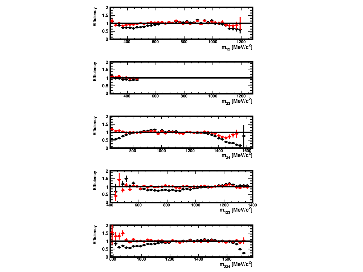
Figure 65: Efficiency in $m_{12}$, $m_{23}$, $m_{34}$, $m_{123}$ and $m_{234}$ in the data generated for this study, in the region $0<m_{23}<480$ MeV$/c^{2}$ and with a tighter selection. Shown are the ratios of the distributions found in the distorted and original samples, with no correction (black) and for decays re-weighted using $\omega_{i}$ weights (red) as explained in Sect. 3.3. The absolute normalisation is arbitrary when the correction is not applied and natural when it is applied (red).

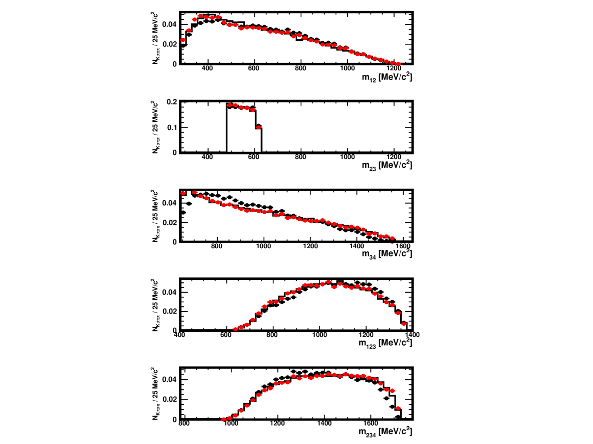
Figure 66: Distributions of $m_{12}$, $m_{23}$, $m_{34}$, $m_{123}$ and $m_{234}$ in the original sample (histogram), in the distorted one obtained with a tighter selection (full black circles) and in the distorted sample where the decays have been re-weighted using the $\omega_{i}$ weights (red), as explained in Sect. 3.3. The data used here are restricted to the region $480<m_{23}<620$ MeV$/c^{2}$. The absolute normalisation is arbitrary when the correction is not applied and natural when it is applied (red).

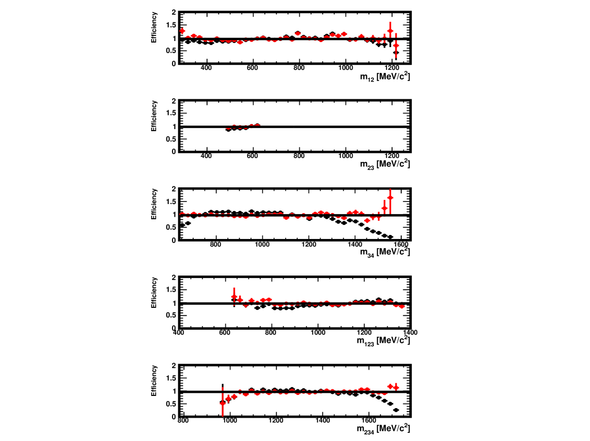
Figure 67: Efficiency in $m_{12}$, $m_{23}$, $m_{34}$, $m_{123}$ and $m_{234}$ in the data generated for this study, in the region $<480m_{23}<620$ MeV$/c^{2}$ and with a tighter selection. Shown are the ratios of the distributions found in the distorted and original samples, with no correction (black) and for decays re-weighted using $\omega_{i}$ weights (red) as explained in Sect. 3.3. The absolute normalisation is arbitrary when the correction is not applied and natural when it is applied (red).

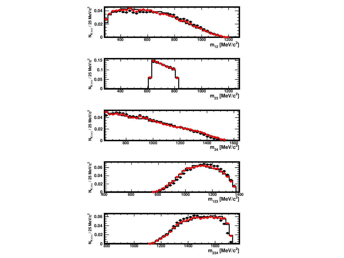
Figure 68: Distributions of $m_{12}$, $m_{23}$, $m_{34}$, $m_{123}$ and $m_{234}$ in the original sample (histogram), in the distorted one obtained with a tighter selection (full black circles) and in the distorted sample where the decays have been re-weighted using the $\omega_{i}$ weights (red), as explained in Sect. 3.3. The data used here are restricted to the region $620<m_{23}<820$ MeV$/c^{2}$. The absolute normalisation is arbitrary when the correction is not applied and natural when it is applied (red).

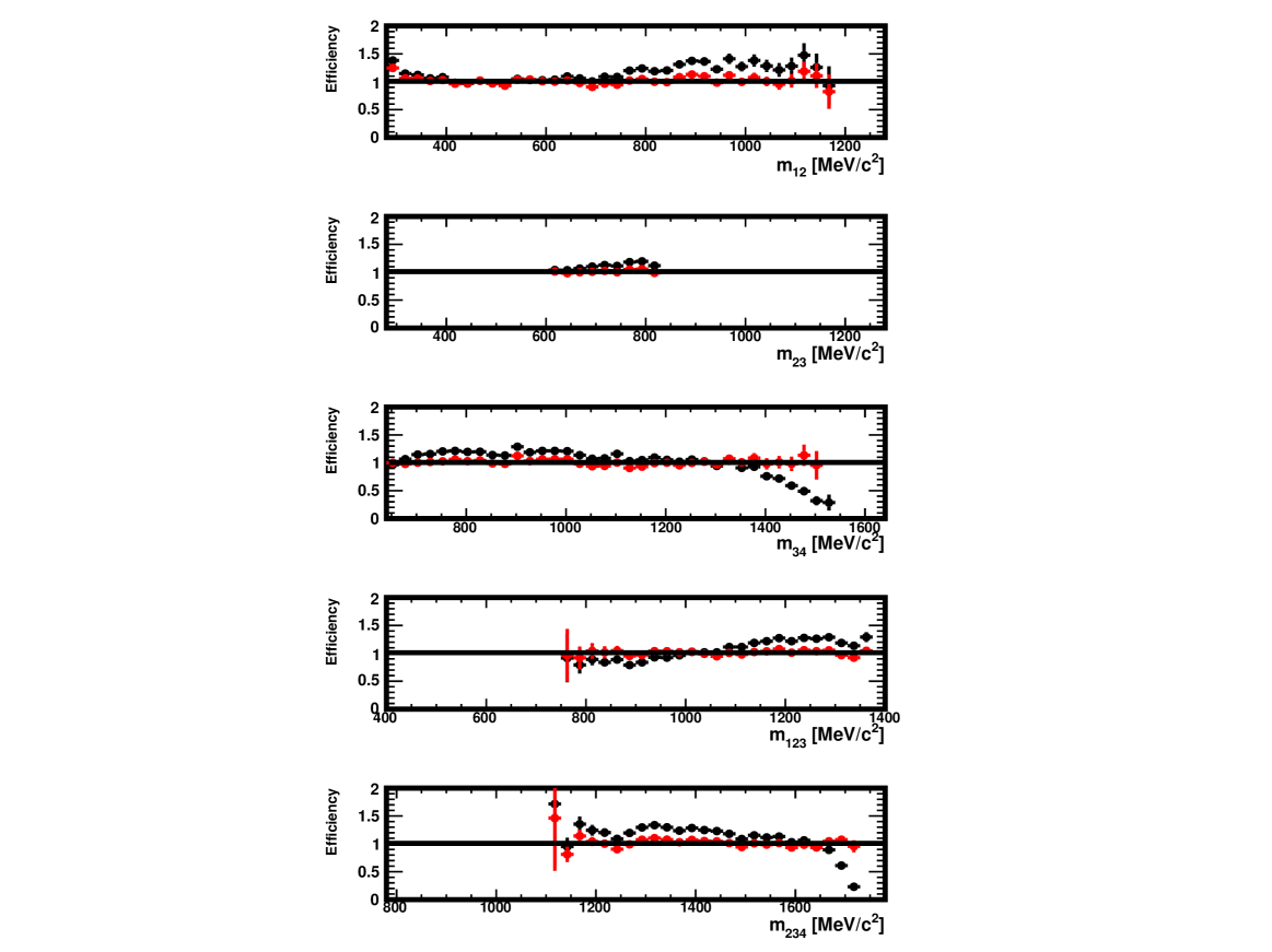
Figure 69: Efficiency in $m_{12}$, $m_{23}$, $m_{34}$, $m_{123}$ and $m_{234}$ in the data generated for this study, in the region $620<m_{23}<820$ MeV$/c^{2}$ and with a tighter selection. Shown are the ratios of the distributions found in the distorted and original samples, with no correction (black) and for decays re-weighted using $\omega_{i}$ weights (red) as explained in Sect. 3.3. The absolute normalisation is arbitrary when the correction is not applied and natural when it is applied (red).

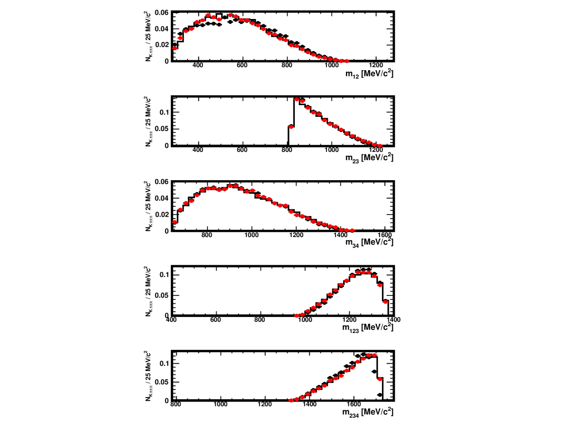
Figure 70: Distributions of $m_{12}$, $m_{23}$, $m_{34}$, $m_{123}$ and $m_{234}$ in the original sample (histogram), in the distorted one obtained with a tighter selection (full black circles) and in the distorted sample where the decays have been re-weighted using the $\omega_{i}$ weights (red), as explained in Sect. 3.3. The data used here are restricted to the region $820<m_{23}$ MeV$/c^{2}$. The absolute normalisation is arbitrary when the correction is not applied and natural when it is applied (red).

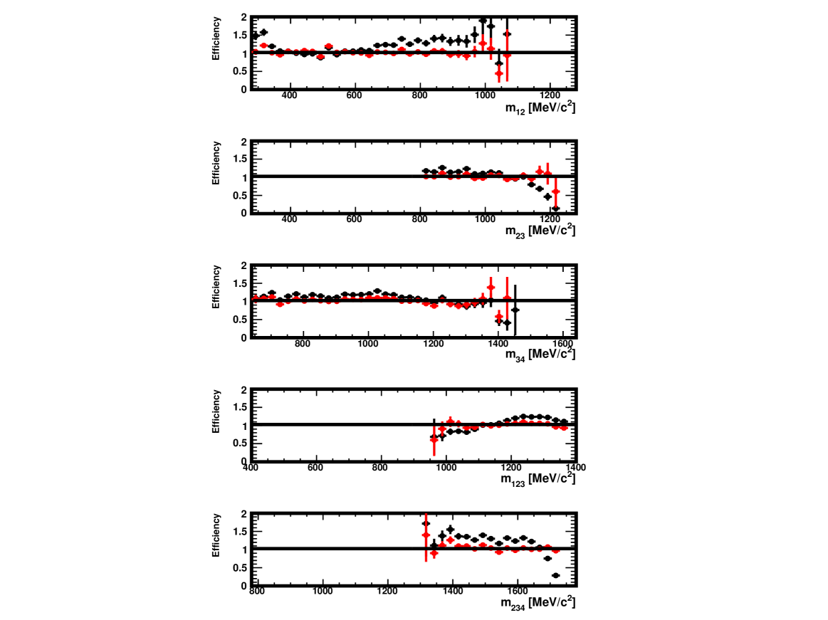
Figure 71: Efficiency in $m_{12}$, $m_{23}$, $m_{34}$, $m_{123}$ and $m_{234}$ in the data generated for this study, in the region $820<m_{23}$ MeV$/c^{2}$ and with a tighter selection. Shown are the ratios of the distributions found in the distorted and original samples, with no correction (black) and for decays re-weighted using $\omega_{i}$ weights (red) as explained in Sect. 3.3. The absolute normalisation is arbitrary when the correction is not applied and natural when it is applied (red).

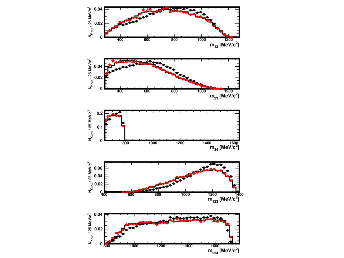
Figure 72: Distributions of $m_{12}$, $m_{23}$, $m_{34}$, $m_{123}$ and $m_{234}$ in the original sample (histogram), in the distorted one obtained with a tighter selection (full black circles) and in the distorted sample where the decays have been re-weighted using the $\omega_{i}$ weights (red), as explained in Sect. 3.3. The data used here are restricted to the region $0<m_{34}<780$ MeV$/c^{2}$. The absolute normalisation is arbitrary when the correction is not applied and natural when it is applied (red).

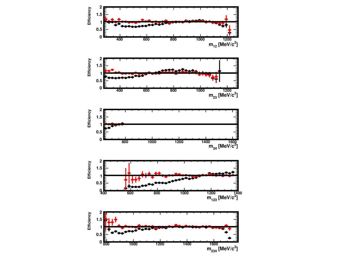
Figure 73: Efficiency in $m_{12}$, $m_{23}$, $m_{34}$, $m_{123}$ and $m_{234}$ in the data generated for this study, in the region $0<m_{34}<780$ MeV$/c^{2}$ and with a tighter selection. Shown are the ratios of the distributions found in the distorted and original samples, with no correction (black) and for decays re-weighted using $\omega_{i}$ weights (red) as explained in Sect. 3.3. The absolute normalisation is arbitrary when the correction is not applied and natural when it is applied (red).

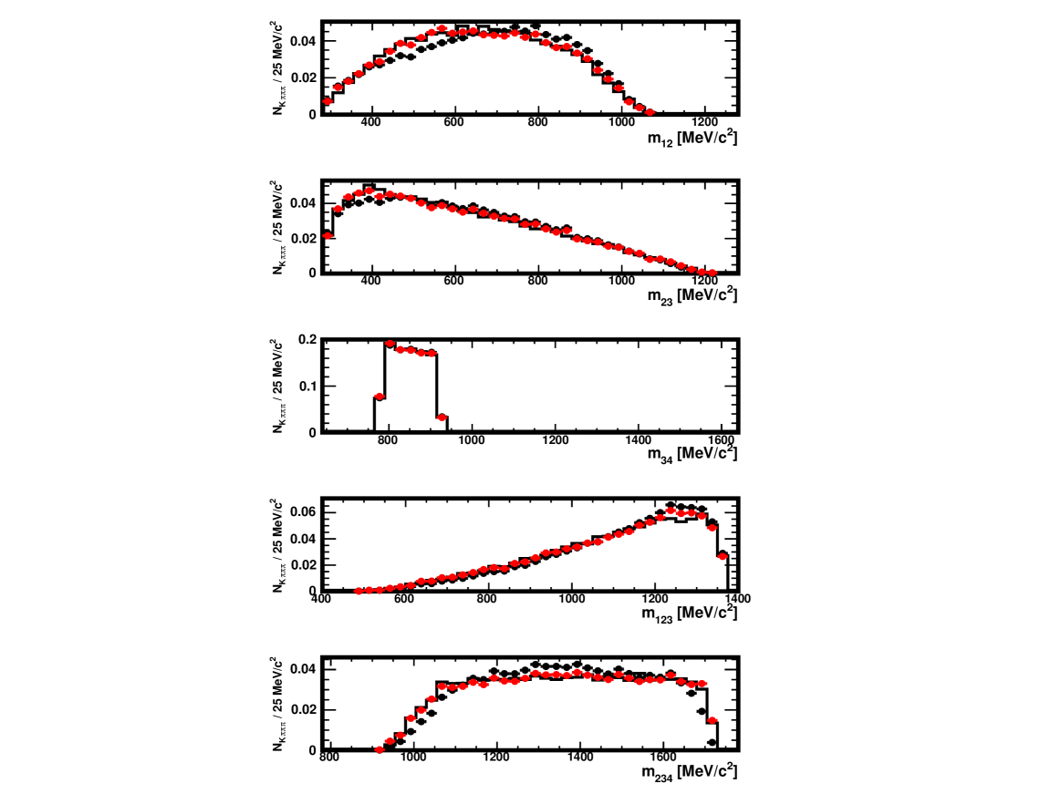
Figure 74: Distributions of $m_{12}$, $m_{23}$, $m_{34}$, $m_{123}$ and $m_{234}$ in the original sample (histogram), in the distorted one obtained with a tighter selection (full black circles) and in the distorted sample where the decays have been re-weighted using the $\omega_{i}$ weights (red), as explained in Sect. 3.3. The data used here are restricted to the region $780<m_{34}<920$ MeV$/c^{2}$. The absolute normalisation is arbitrary when the correction is not applied and natural when it is applied (red).

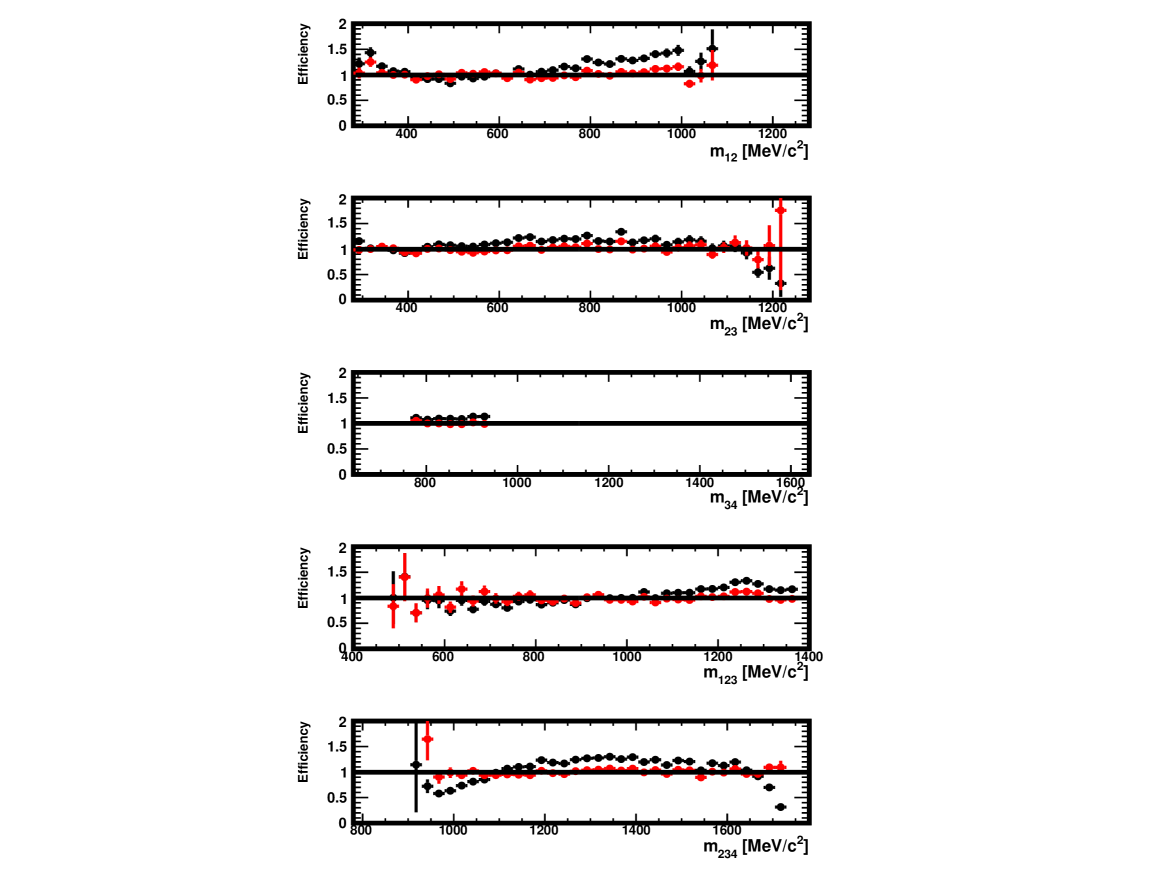
Figure 75: Efficiency in $m_{12}$, $m_{23}$, $m_{34}$, $m_{123}$ and $m_{234}$ in the data generated for this study, in the region $<780m_{34}<920$ MeV$/c^{2}$ and with a tighter selection. Shown are the ratios of the distributions found in the distorted and original samples, with no correction (black) and for decays re-weighted using $\omega_{i}$ weights (red) as explained in Sect. 3.3. The absolute normalisation is arbitrary when the correction is not applied and natural when it is applied (red).

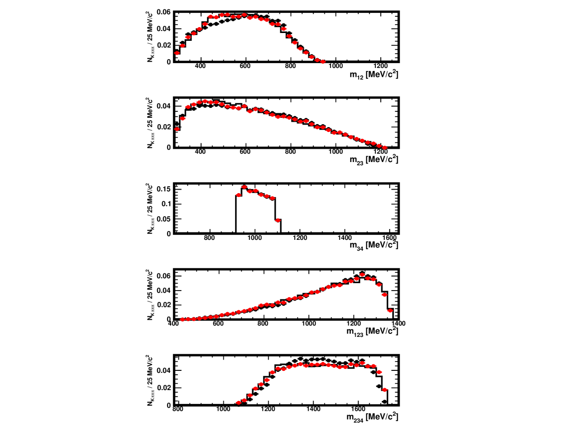
Figure 76: Distributions of $m_{12}$, $m_{23}$, $m_{34}$, $m_{123}$ and $m_{234}$ in the original sample (histogram), in the distorted one obtained with a tighter selection (full black circles) and in the distorted sample where the decays have been re-weighted using the $\omega_{i}$ weights (red), as explained in Sect. 3.3. The data used here are restricted to the region $920<m_{34}<1100$ MeV$/c^{2}$. The absolute normalisation is arbitrary when the correction is not applied and natural when it is applied (red).

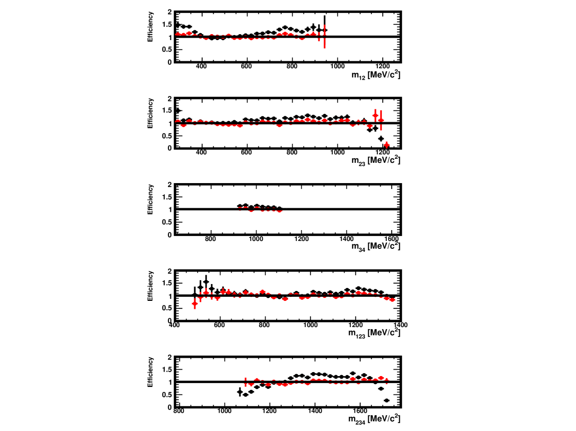
Figure 77: Efficiency in $m_{12}$, $m_{23}$, $m_{34}$, $m_{123}$ and $m_{234}$ in the data generated for this study, in the region $920<m_{34}<1100$ MeV$/c^{2}$ and with a tighter selection. Shown are the ratios of the distributions found in the distorted and original samples, with no correction (black) and for decays re-weighted using $\omega_{i}$ weights (red) as explained in Sect. 3.3. The absolute normalisation is arbitrary when the correction is not applied and natural when it is applied (red).

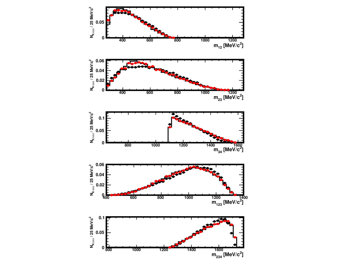
Figure 78: Distributions of $m_{12}$, $m_{23}$, $m_{34}$, $m_{123}$ and $m_{234}$ in the original sample (histogram), in the distorted one obtained with a tighter selection (full black circles) and in the distorted sample where the decays have been re-weighted using the $\omega_{i}$ weights (red), as explained in Sect. 3.3. The data used here are restricted to the region $1100<m_{34}$ MeV$/c^{2}$. The absolute normalisation is arbitrary when the correction is not applied and natural when it is applied (red).

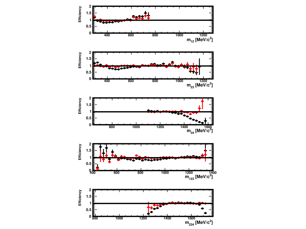
Figure 79: Efficiency in $m_{12}$, $m_{23}$, $m_{34}$, $m_{123}$ and $m_{234}$ in the data generated for this study, in the region $1100<m_{34}$ MeV$/c^{2}$ and with a tighter selection. Shown are the ratios of the distributions found in the distorted and original samples, with no correction (black) and for decays re-weighted using $\omega_{i}$ weights (red) as explained in Sect. 3.3. The absolute normalisation is arbitrary when the correction is not applied and natural when it is applied (red).

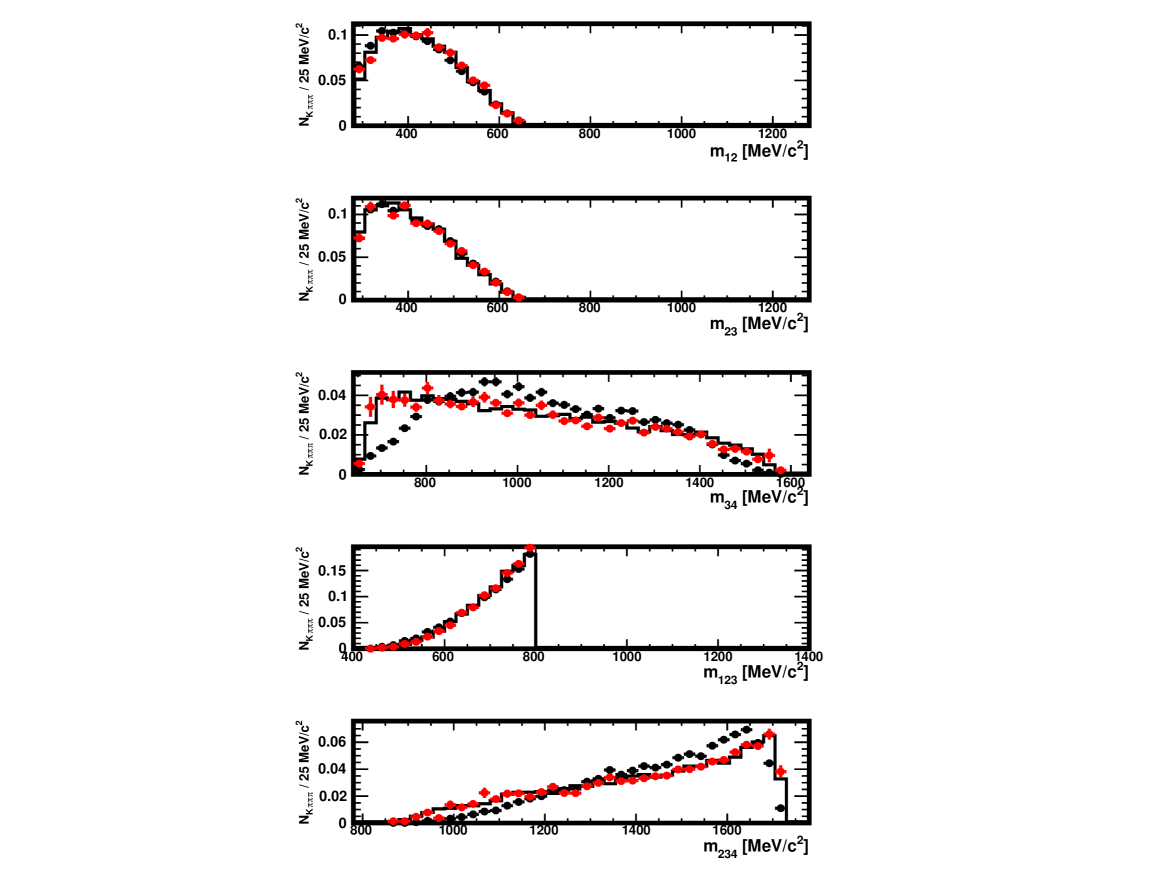
Figure 80: Distributions of $m_{12}$, $m_{23}$, $m_{34}$, $m_{123}$ and $m_{234}$ in the original sample (histogram), in the distorted one obtained with a tighter selection (full black circles) and in the distorted sample where the decays have been re-weighted using the $\omega_{i}$ weights (red), as explained in Sect. 3.3. The data used here are restricted to the region $0<m_{123}<800$ MeV$/c^{2}$. The absolute normalisation is arbitrary when the correction is not applied and natural when it is applied (red).

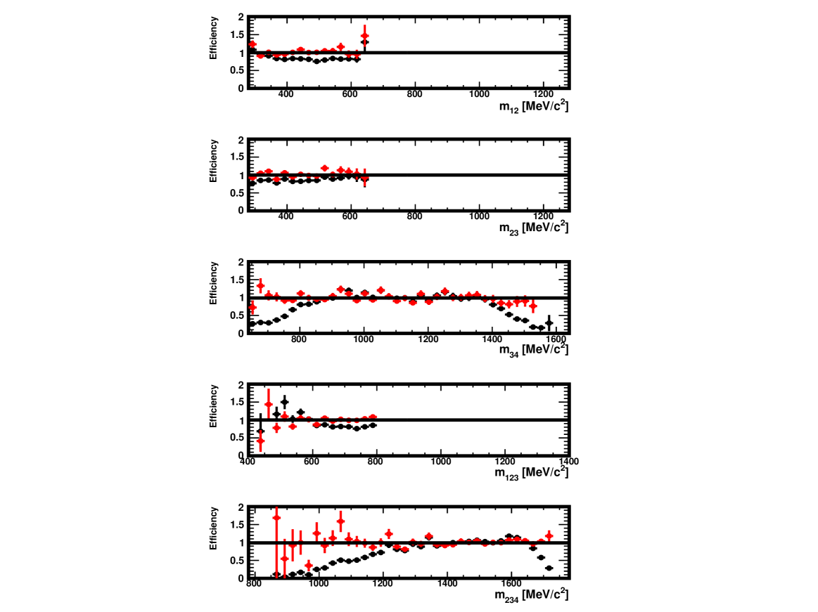
Figure 81: Efficiency in $m_{12}$, $m_{23}$, $m_{34}$, $m_{123}$ and $m_{234}$ in the data generated for this study, in the region $0<m_{123}<800$ MeV$/c^{2}$ and with a tighter selection. Shown are the ratios of the distributions found in the distorted and original samples, with no correction (black) and for decays re-weighted using $\omega_{i}$ weights (red) as explained in Sect. 3.3. The absolute normalisation is arbitrary when the correction is not applied and natural when it is applied (red).

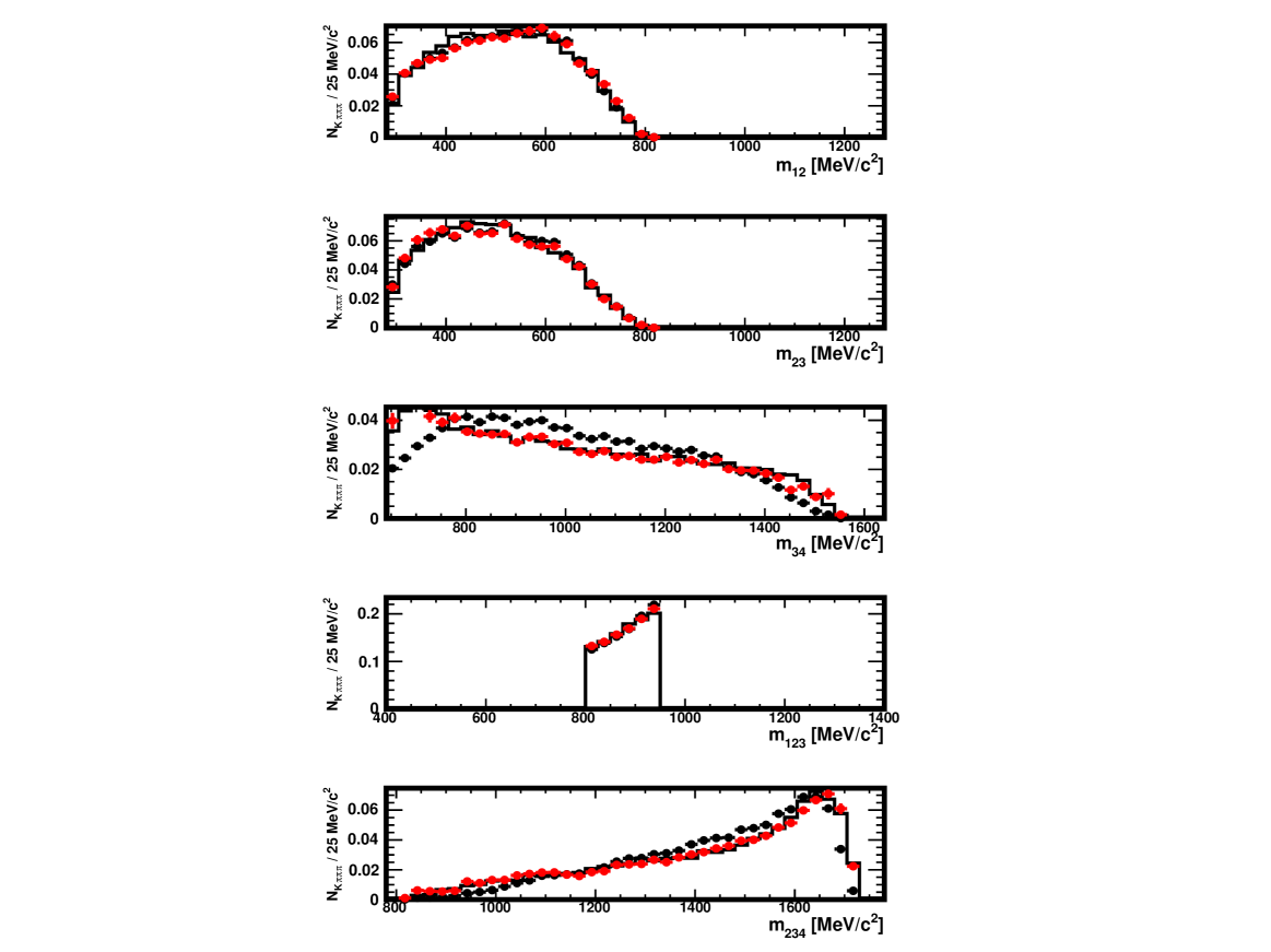
Figure 82: Distributions of $m_{12}$, $m_{23}$, $m_{123}$, $m_{123}$ and $m_{234}$ in the original sample (histogram), in the distorted one obtained with a tighter selection (full black circles) and in the distorted sample where the decays have been re-weighted using the $\omega_{i}$ weights (red), as explained in Sect. 3.3. The data used here are restricted to the region $800<m_{123}<950$ MeV$/c^{2}$. The absolute normalisation is arbitrary when the correction is not applied and natural when it is applied (red).

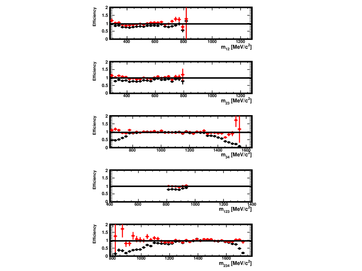
Figure 83: Efficiency in $m_{12}$, $m_{23}$, $m_{34}$, $m_{123}$ and $m_{234}$ in the data generated for this study, in the region $<800m_{123}<950$ MeV$/c^{2}$ and with a tighter selection. Shown are the ratios of the distributions found in the distorted and original samples, with no correction (black) and for decays re-weighted using $\omega_{i}$ weights (red) as explained in Sect. 3.3. The absolute normalisation is arbitrary when the correction is not applied and natural when it is applied (red).

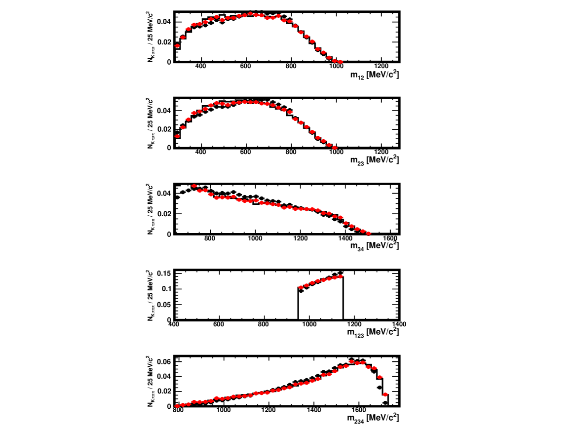
Figure 84: Distributions of $m_{12}$, $m_{23}$, $m_{34}$, $m_{123}$ and $m_{234}$ in the original sample (histogram), in the distorted one obtained with a tighter selection (full black circles) and in the distorted sample where the decays have been re-weighted using the $\omega_{i}$ weights (red), as explained in Sect. 3.3. The data used here are restricted to the region $950<m_{123}<1150$ MeV$/c^{2}$. The absolute normalisation is arbitrary when the correction is not applied and natural when it is applied (red).

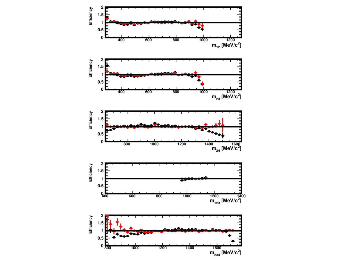
Figure 85: Efficiency in $m_{12}$, $m_{23}$, $m_{34}$, $m_{123}$ and $m_{234}$ in the data generated for this study, in the region $950<m_{123}<1150$ MeV$/c^{2}$ and with a tighter selection. Shown are the ratios of the distributions found in the distorted and original samples, with no correction (black) and for decays re-weighted using $\omega_{i}$ weights (red) as explained in Sect. 3.3. The absolute normalisation is arbitrary when the correction is not applied and natural when it is applied (red).

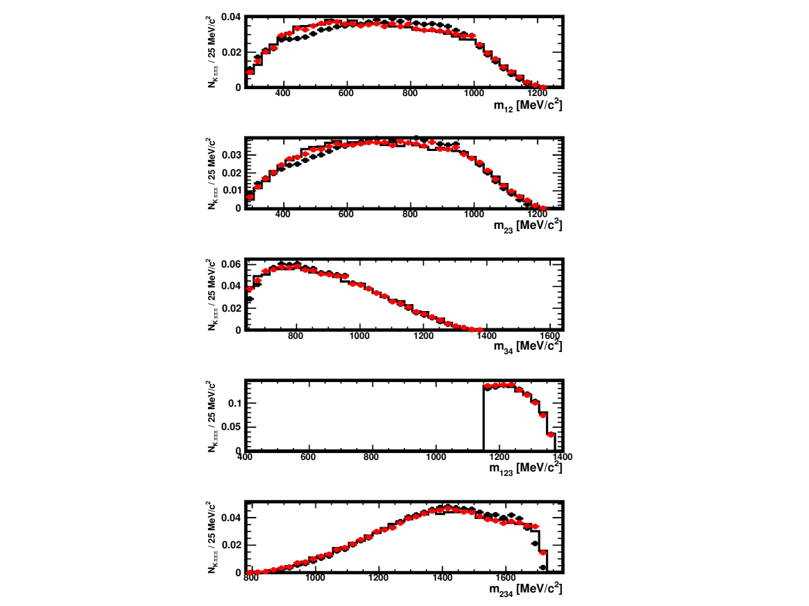
Figure 86: Distributions of $m_{12}$, $m_{23}$, $m_{34}$, $m_{123}$ and $m_{234}$ in the original sample (histogram), in the distorted one obtained with a tighter selection (full black circles) and in the distorted sample where the decays have been re-weighted using the $\omega_{i}$ weights (red), as explained in Sect. 3.3. The data used here are restricted to the region $1150<m_{123}$ MeV$/c^{2}$. The absolute normalisation is arbitrary when the correction is not applied and natural when it is applied (red).

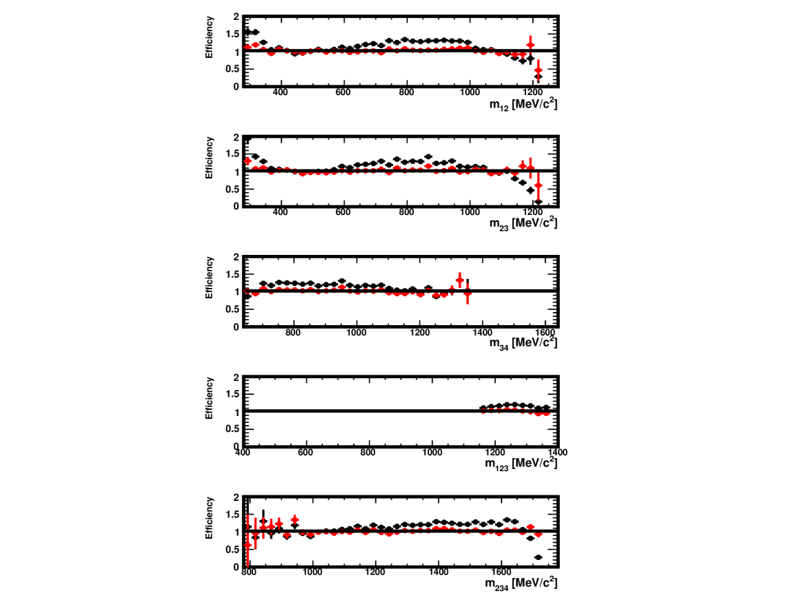
Figure 87: Efficiency in $m_{12}$, $m_{23}$, $m_{34}$, $m_{123}$ and $m_{234}$ in the data generated for this study, in the region $1150<m_{123}$ MeV$/c^{2}$ and with a tighter selection. Shown are the ratios of the distributions found in the distorted and original samples, with no correction (black) and for decays re-weighted using $\omega_{i}$ weights (red) as explained in Sect. 3.3. The absolute normalisation is arbitrary when the correction is not applied and natural when it is applied (red).

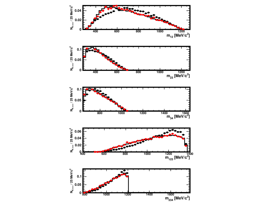
Figure 88: Distributions of $m_{12}$, $m_{23}$, $m_{34}$, $m_{123}$ and $m_{234}$ in the original sample (histogram), in the distorted one obtained with a tighter selection (full black circles) and in the distorted sample where the decays have been re-weighted using the $\omega_{i}$ weights (red), as explained in Sect. 3.3. The data used here are restricted to the region $0<m_{234}<800$ MeV$/c^{2}$. The absolute normalisation is arbitrary when the correction is not applied and natural when it is applied (red).

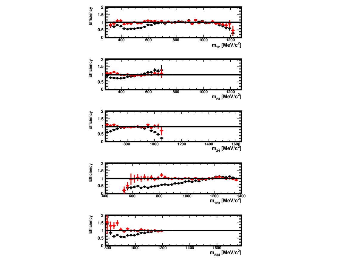
Figure 89: Efficiency in $m_{12}$, $m_{23}$, $m_{34}$, $m_{123}$ and $m_{234}$ in the data generated for this study, in the region $0<m_{234}<800$ MeV$/c^{2}$ and with a tighter selection. Shown are the ratios of the distributions found in the distorted and original samples, with no correction (black) and for decays re-weighted using $\omega_{i}$ weights (red) as explained in Sect. 3.3. The absolute normalisation is arbitrary when the correction is not applied and natural when it is applied (red).

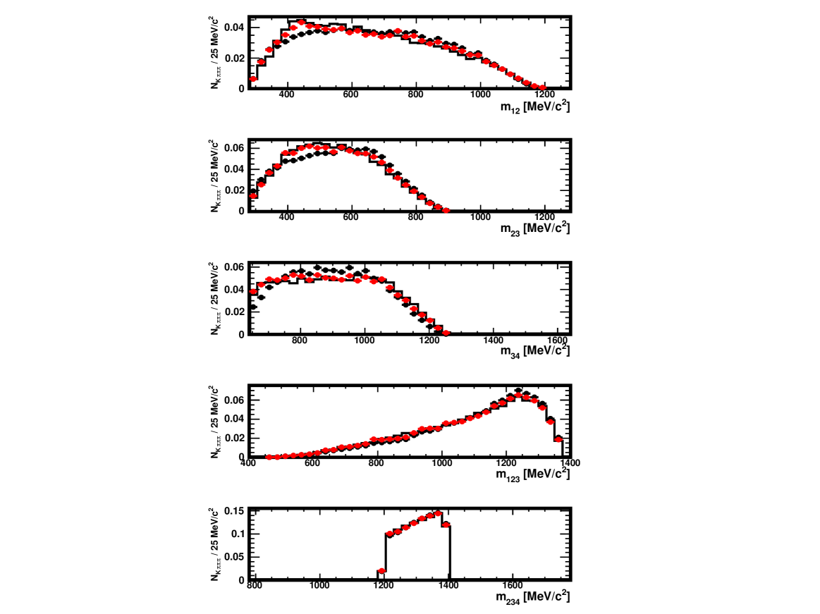
Figure 90: Distributions of $m_{12}$, $m_{23}$, $m_{123}$, $m_{123}$ and $m_{234}$ in the original sample (histogram), in the distorted one obtained with a tighter selection (full black circles) and in the distorted sample where the decays have been re-weighted using the $\omega_{i}$ weights (red), as explained in Sect. 3.3. The data used here are restricted to the region $800<m_{234}<950$ MeV$/c^{2}$. The absolute normalisation is arbitrary when the correction is not applied and natural when it is applied (red).

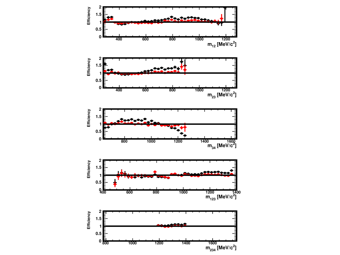
Figure 91: Efficiency in $m_{12}$, $m_{23}$, $m_{34}$, $m_{123}$ and $m_{234}$ in the data generated for this study, in the region $<800m_{234}<950$ MeV$/c^{2}$ and with a tighter selection. Shown are the ratios of the distributions found in the distorted and original samples, with no correction (black) and for decays re-weighted using $\omega_{i}$ weights (red) as explained in Sect. 3.3. The absolute normalisation is arbitrary when the correction is not applied and natural when it is applied (red).

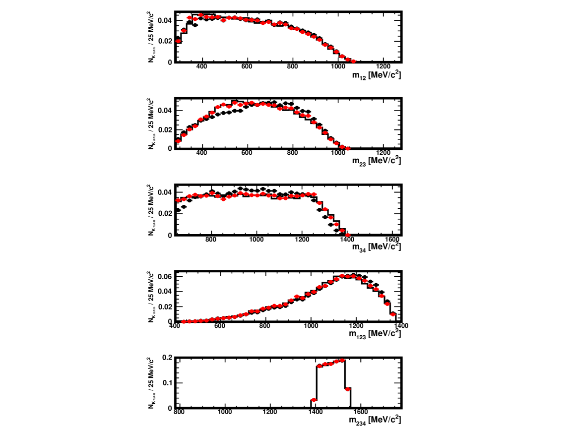
Figure 92: Distributions of $m_{12}$, $m_{23}$, $m_{34}$, $m_{123}$ and $m_{234}$ in the original sample (histogram), in the distorted one obtained with a tighter selection (full black circles) and in the distorted sample where the decays have been re-weighted using the $\omega_{i}$ weights (red), as explained in Sect. 3.3. The data used here are restricted to the region $950<m_{234}<1150$ MeV$/c^{2}$. The absolute normalisation is arbitrary when the correction is not applied and natural when it is applied (red).

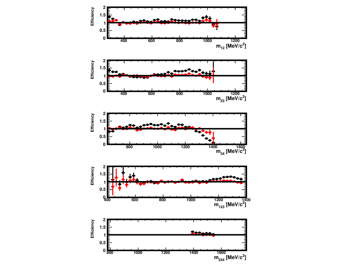
Figure 93: Efficiency in $m_{12}$, $m_{23}$, $m_{34}$, $m_{123}$ and $m_{234}$ in the data generated for this study, in the region $950<m_{234}<1150$ MeV$/c^{2}$ and with a tighter selection. Shown are the ratios of the distributions found in the distorted and original samples, with no correction (black) and for decays re-weighted using $\omega_{i}$ weights (red) as explained in Sect. 3.3. The absolute normalisation is arbitrary when the correction is not applied and natural when it is applied (red).

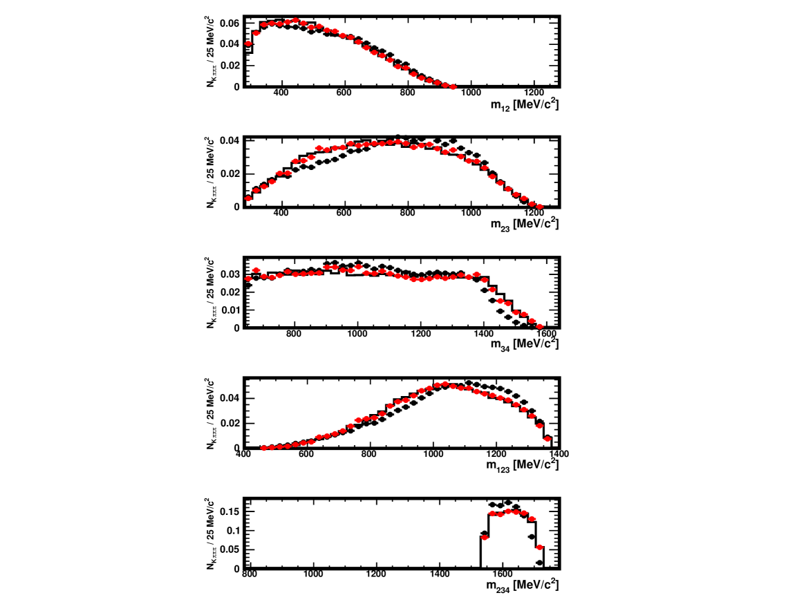
Figure 94: Distributions of $m_{12}$, $m_{23}$, $m_{34}$, $m_{123}$ and $m_{234}$ in the original sample (histogram), in the distorted one obtained with a tighter selection (full black circles) and in the distorted sample where the decays have been re-weighted using the $\omega_{i}$ weights (red), as explained in Sect. 3.3. The data used here are restricted to the region $1150<m_{234}$ MeV$/c^{2}$. The absolute normalisation is arbitrary when the correction is not applied and natural when it is applied (red).

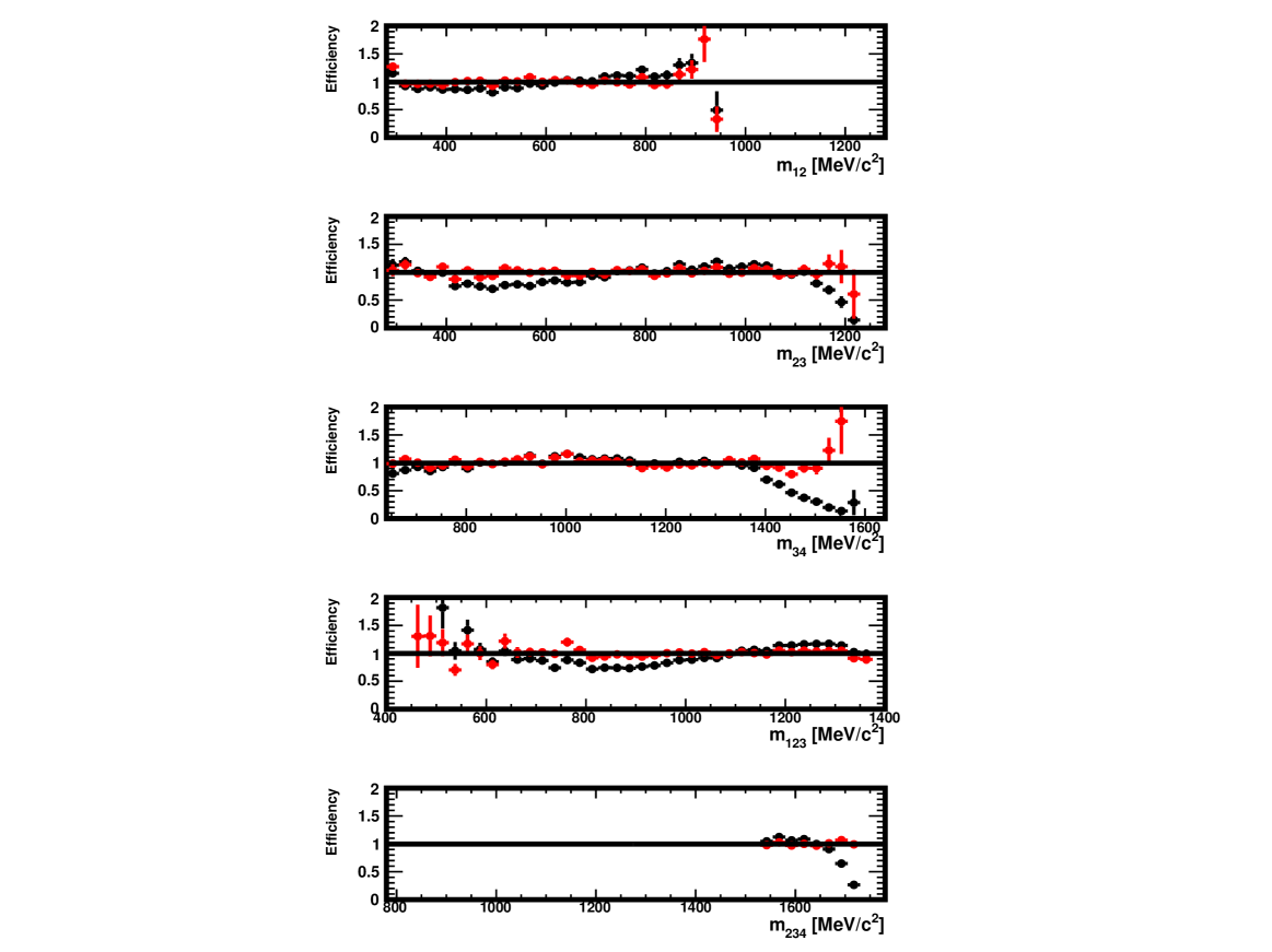
Figure 95: Efficiency in $m_{12}$, $m_{23}$, $m_{34}$, $m_{123}$ and $m_{234}$ in the data generated for this study, in the region $1150<m_{234}$ MeV$/c^{2}$ and with a tighter selection. Shown are the ratios of the distributions found in the distorted and original samples, with no correction (black) and for decays re-weighted using $\omega_{i}$ weights (red) as explained in Sect. 3.3. The absolute normalisation is arbitrary when the correction is not applied and natural when it is applied (red).

Appendix B Additional figures related to the ${{B}^{0}}\!\rightarrow{{K}^{*0}}(\rightarrow{{K}^{+}}{{\pi}^{-}}){\mu^{+}}{\mu^{-}}$ test case

Figure 96: Efficiency in $q^{2}$, cos$\theta_{l}$, cos$\theta_{K}$ and $\phi$ in the data generated for the present study, in the region $0.1<q^{2}<0.98$ GeV${}^{2}/c^{4}$. Shown are the ratios of the distributions found in the distorted and original samples, with no correction (black) and for decays re-weighted using $\omega_{i}$ weights (red) as explained in Sect. 4.3. The absolute normalisation is arbitrary when the correction is not applied and natural when it is applied (red).

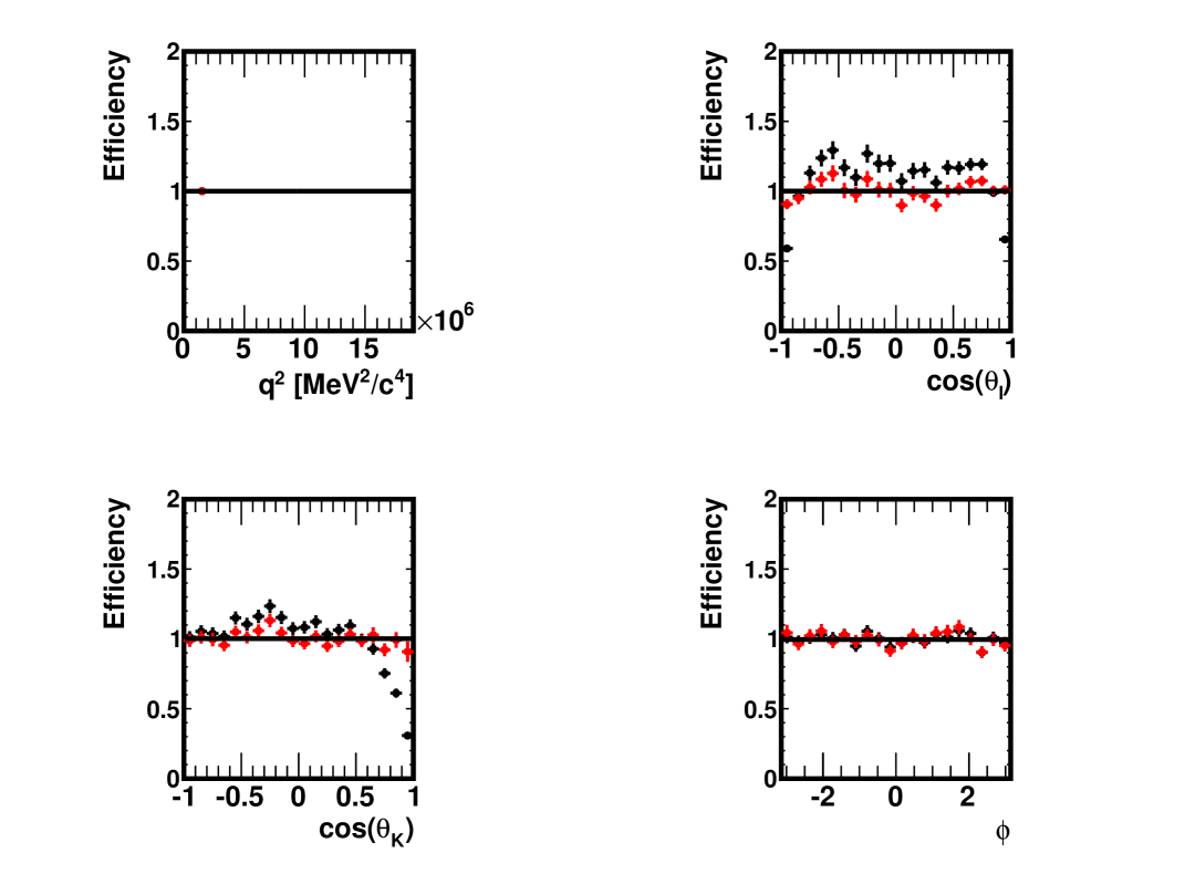
Figure 97: Efficiency in $q^{2}$, cos$\theta_{l}$, cos$\theta_{K}$ and $\phi$ in the data generated for the present study, in the region $0.98<q^{2}<2.0$ GeV${}^{2}/c^{4}$. Shown are the ratios of the distributions found in the distorted and original samples, with no correction (black) and for decays re-weighted using $\omega_{i}$ weights (red) as explained in Sect. 4.3. The absolute normalisation is arbitrary when the correction is not applied and natural when it is applied (red).

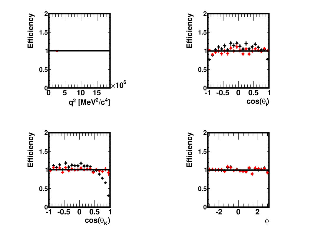
Figure 98: Efficiency in $q^{2}$, cos$\theta_{l}$, cos$\theta_{K}$ and $\phi$ in the data generated for the present study, in the region $2.0<q^{2}<3.0$ GeV${}^{2}/c^{4}$. Shown are the ratios of the distributions found in the distorted and original samples, with no correction (black) and for decays re-weighted using $\omega_{i}$ weights (red) as explained in Sect. 4.3. The absolute normalisation is arbitrary when the correction is not applied and natural when it is applied (red).

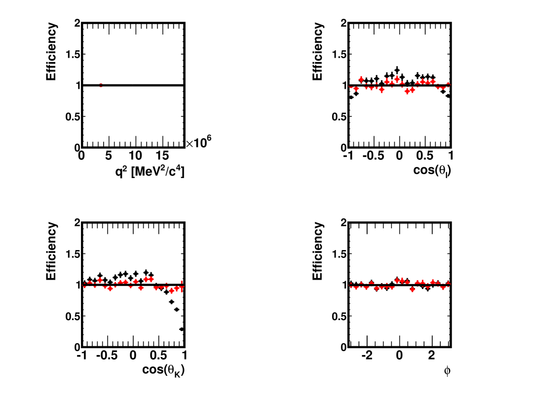
Figure 99: Efficiency in $q^{2}$, cos$\theta_{l}$, cos$\theta_{K}$ and $\phi$ in the data generated for the present study, in the region $3.0<q^{2}<4.0$ GeV${}^{2}/c^{4}$. Shown are the ratios of the distributions found in the distorted and original samples, with no correction (black) and for decays re-weighted using $\omega_{i}$ weights (red) as explained in Sect. 4.3. The absolute normalisation is arbitrary when the correction is not applied and natural when it is applied (red).

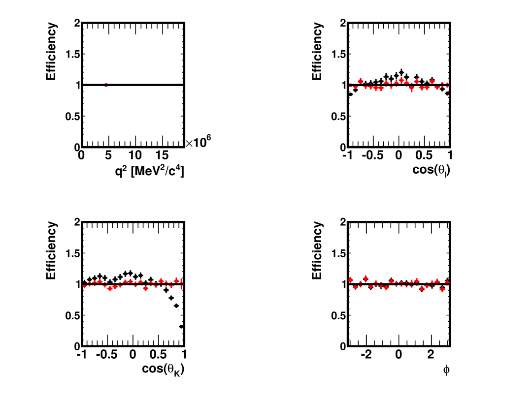
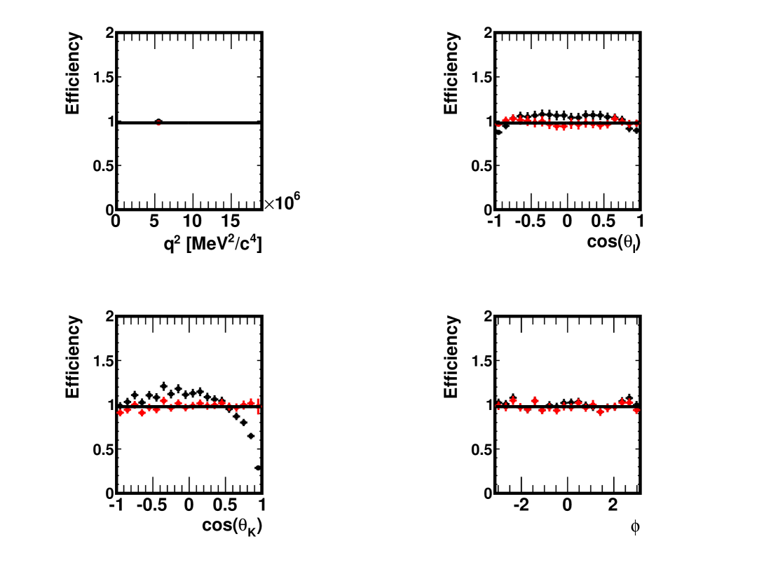
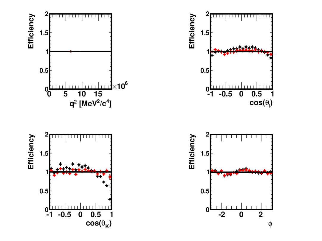
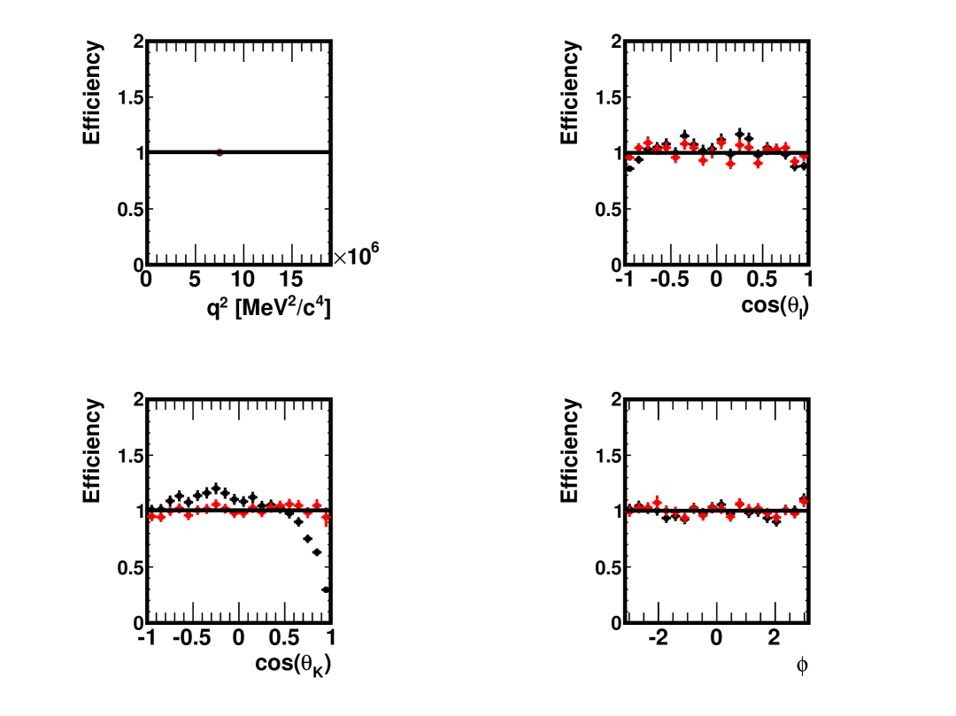
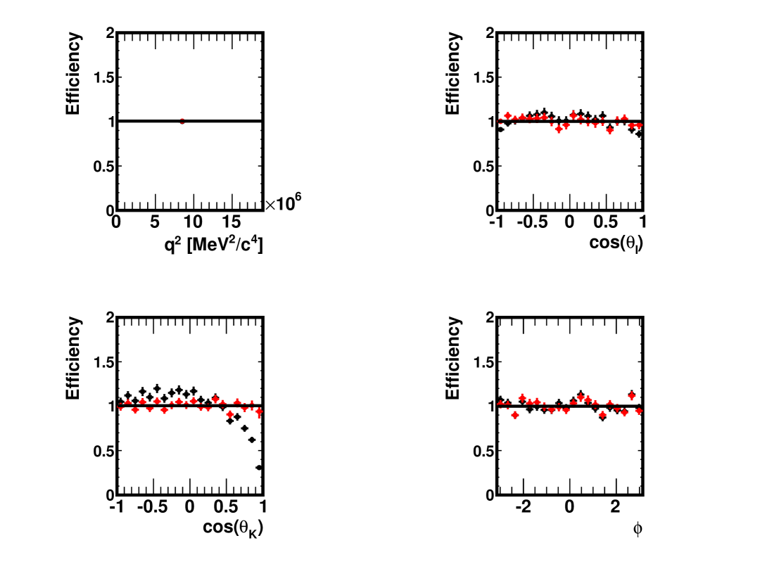
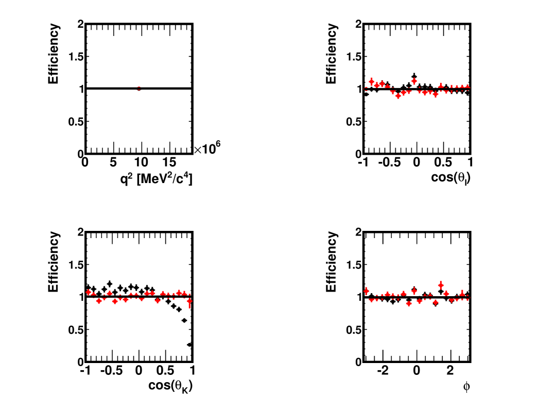
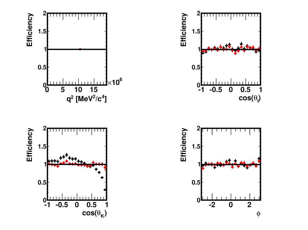
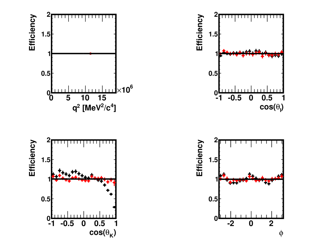
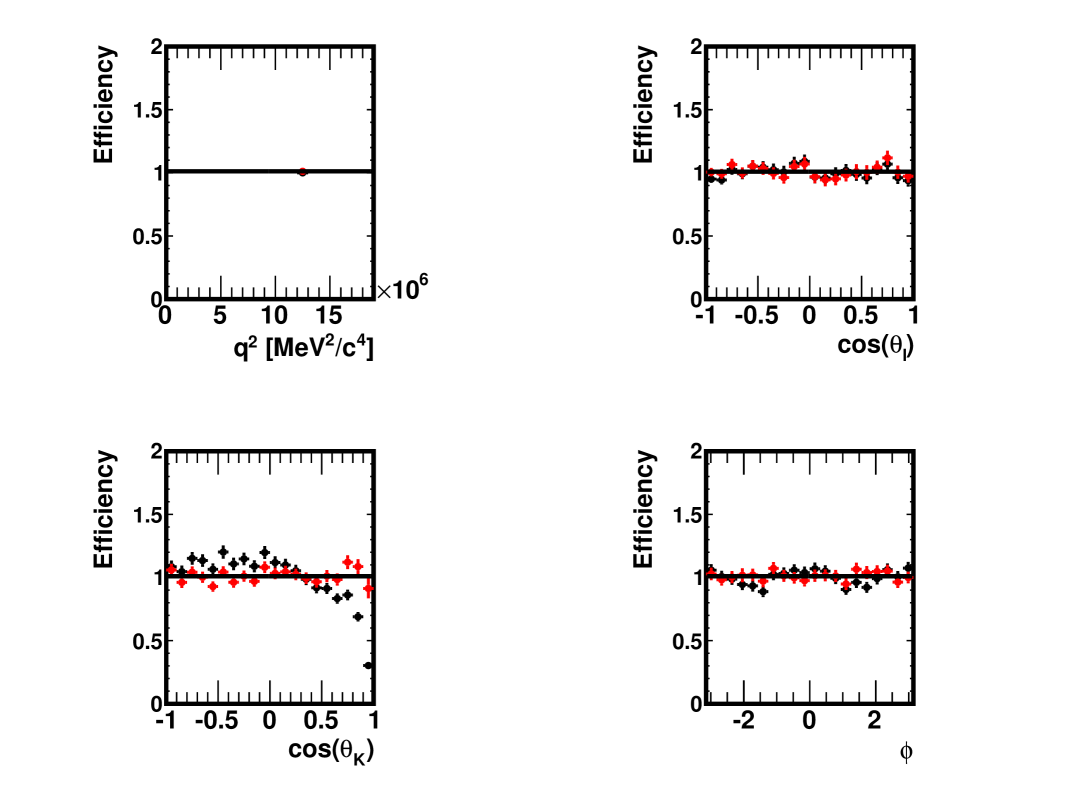
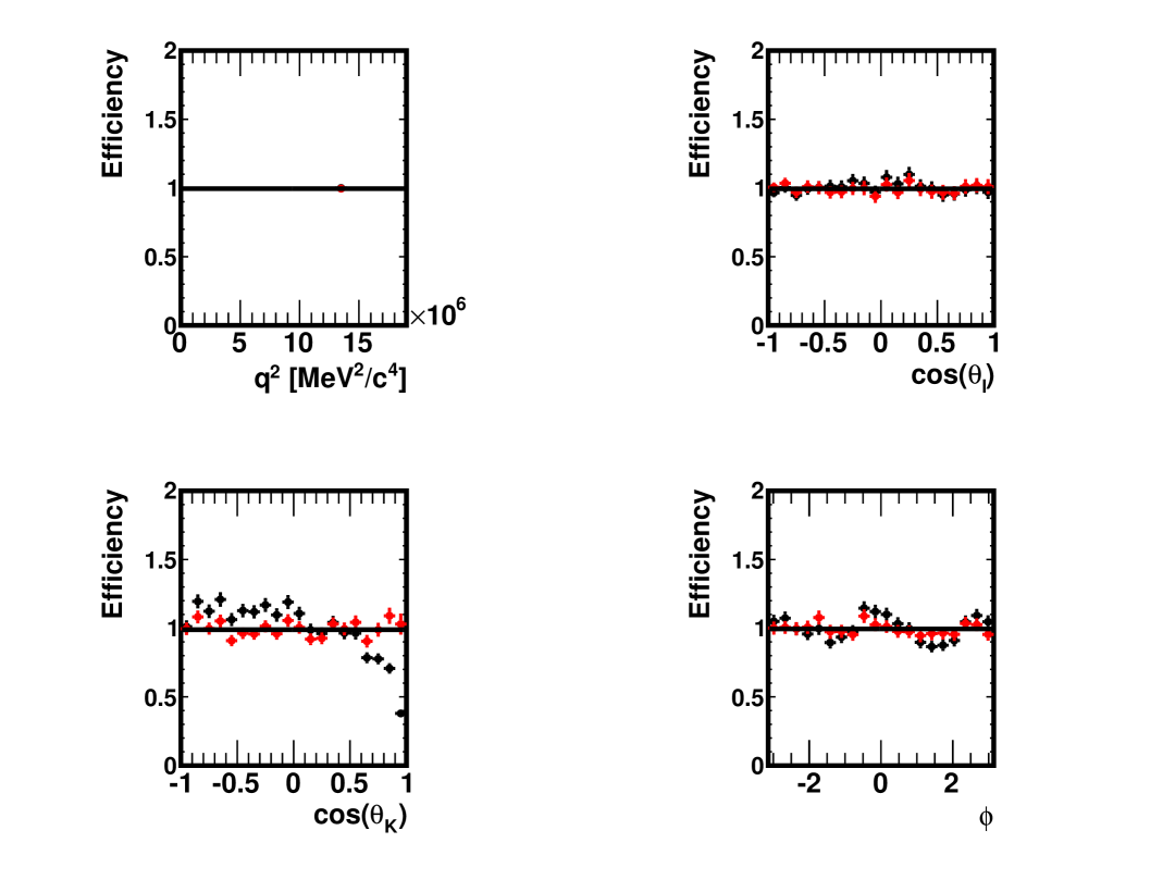
Figure 100: Efficiency in $q^{2}$, cos$\theta_{l}$, cos$\theta_{K}$ and $\phi$ in the data generated for the present study, in the region $4.0<q^{2}<5.0$ GeV${}^{2}/c^{4}$. Shown are the ratios of the distributions found in the distorted and original samples, with no correction (black) and for decays re-weighted using $\omega_{i}$ weights (red) as explained in Sect. 4.3. The absolute normalisation is arbitrary when the correction is not applied and natural when it is applied (red).

Figure 101: Efficiency in $q^{2}$, cos$\theta_{l}$, cos$\theta_{K}$ and $\phi$ in the data generated for the present study, in the region $5.0<q^{2}<6.0$ GeV${}^{2}/c^{4}$. Shown are the ratios of the distributions found in the distorted and original samples, with no correction (black) and for decays re-weighted using $\omega_{i}$ weights (red) as explained in Sect. 4.3. The absolute normalisation is arbitrary when the correction is not applied and natural when it is applied (red).

Figure 102: Efficiency in $q^{2}$, cos$\theta_{l}$, cos$\theta_{K}$ and $\phi$ in the data generated for the present study, in the region $6.0<q^{2}<7.0$ GeV${}^{2}/c^{4}$. Shown are the ratios of the distributions found in the distorted and original samples, with no correction (black) and for decays re-weighted using $\omega_{i}$ weights (red) as explained in Sect. 4.3. The absolute normalisation is arbitrary when the correction is not applied and natural when it is applied (red).

Figure 103: Efficiency in $q^{2}$, cos$\theta_{l}$, cos$\theta_{K}$ and $\phi$ in the data generated for the present study, in the region $7.0<q^{2}<8.0$ GeV${}^{2}/c^{4}$. Shown are the ratios of the distributions found in the distorted and original samples, with no correction (black) and for decays re-weighted using $\omega_{i}$ weights (red) as explained in Sect. 4.3. The absolute normalisation is arbitrary when the correction is not applied and natural when it is applied (red).

Figure 104: Efficiency in $q^{2}$, cos$\theta_{l}$, cos$\theta_{K}$ and $\phi$ in the data generated for the present study, in the region $8.0<q^{2}<9.0$ GeV${}^{2}/c^{4}$. Shown are the ratios of the distributions found in the distorted and original samples, with no correction (black) and for decays re-weighted using $\omega_{i}$ weights (red) as explained in Sect. 4.3. The absolute normalisation is arbitrary when the correction is not applied and natural when it is applied (red).

Figure 105: Efficiency in $q^{2}$, cos$\theta_{l}$, cos$\theta_{K}$ and $\phi$ in the data generated for the present study, in the region $9.0<q^{2}<10.0$ GeV${}^{2}/c^{4}$. Shown are the ratios of the distributions found in the distorted and original samples, with no correction (black) and for decays re-weighted using $\omega_{i}$ weights (red) as explained in Sect. 4.3. The absolute normalisation is arbitrary when the correction is not applied and natural when it is applied (red).

Figure 106: Efficiency in $q^{2}$, cos$\theta_{l}$, cos$\theta_{K}$ and $\phi$ in the data generated for the present study, in the region $10.0<q^{2}<11.0$ GeV${}^{2}/c^{4}$. Shown are the ratios of the distributions found in the distorted and original samples, with no correction (black) and for decays re-weighted using $\omega_{i}$ weights (red) as explained in Sect. 4.3. The absolute normalisation is arbitrary when the correction is not applied and natural when it is applied (red).

Figure 107: Efficiency in $q^{2}$, cos$\theta_{l}$, cos$\theta_{K}$ and $\phi$ in the data generated for the present study, in the region $11.0<q^{2}<12.0$ GeV${}^{2}/c^{4}$. Shown are the ratios of the distributions found in the distorted and original samples, with no correction (black) and for decays re-weighted using $\omega_{i}$ weights (red) as explained in Sect. 4.3. The absolute normalisation is arbitrary when the correction is not applied and natural when it is applied (red).

Figure 108: Efficiency in $q^{2}$, cos$\theta_{l}$, cos$\theta_{K}$ and $\phi$ in the data generated for the present study, in the region $12.0<q^{2}<13.0$ GeV${}^{2}/c^{4}$. Shown are the ratios of the distributions found in the distorted and original samples, with no correction (black) and for decays re-weighted using $\omega_{i}$ weights (red) as explained in Sect. 4.3. The absolute normalisation is arbitrary when the correction is not applied and natural when it is applied (red).

Figure 109: Efficiency in $q^{2}$, cos$\theta_{l}$, cos$\theta_{K}$ and $\phi$ in the data generated for the present study, in the region $13.0<q^{2}<14.0$ GeV${}^{2}/c^{4}$. Shown are the ratios of the distributions found in the distorted and original samples, with no correction (black) and for decays re-weighted using $\omega_{i}$ weights (red) as explained in Sect. 4.3. The absolute normalisation is arbitrary when the correction is not applied and natural when it is applied (red).

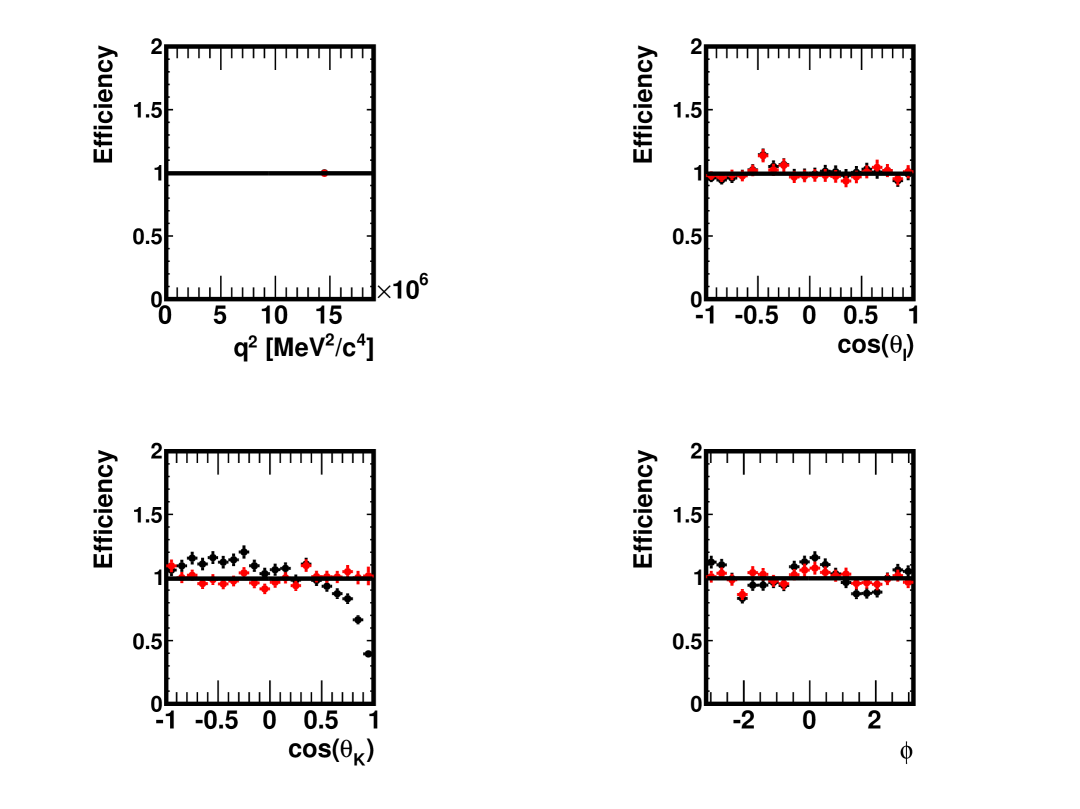
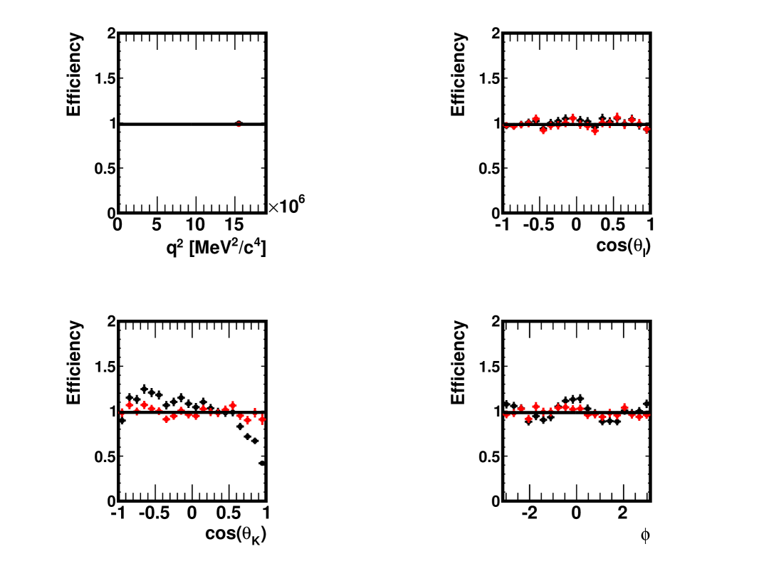
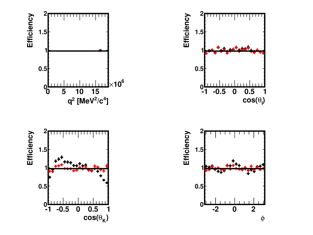
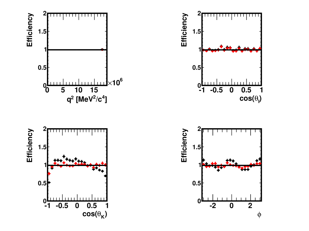
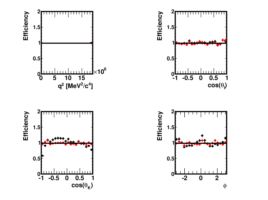
Figure 110: Efficiency in $q^{2}$, cos$\theta_{l}$, cos$\theta_{K}$ and $\phi$ in the data generated for the present study, in the region $14.0<q^{2}<15.0$ GeV${}^{2}/c^{4}$. Shown are the ratios of the distributions found in the distorted and original samples, with no correction (black) and for decays re-weighted using $\omega_{i}$ weights (red) as explained in Sect. 4.3. The absolute normalisation is arbitrary when the correction is not applied and natural when it is applied (red).

Figure 111: Efficiency in $q^{2}$, cos$\theta_{l}$, cos$\theta_{K}$ and $\phi$ in the data generated for the present study, in the region $15.0<q^{2}<16.0$ GeV${}^{2}/c^{4}$. Shown are the ratios of the distributions found in the distorted and original samples, with no correction (black) and for decays re-weighted using $\omega_{i}$ weights (red) as explained in Sect. 4.3. The absolute normalisation is arbitrary when the correction is not applied and natural when it is applied (red).

Figure 112: Efficiency in $q^{2}$, cos$\theta_{l}$, cos$\theta_{K}$ and $\phi$ in the data generated for the present study, in the region $16.0<q^{2}<17.0$ GeV${}^{2}/c^{4}$. Shown are the ratios of the distributions found in the distorted and original samples, with no correction (black) and for decays re-weighted using $\omega_{i}$ weights (red) as explained in Sect. 4.3. The absolute normalisation is arbitrary when the correction is not applied and natural when it is applied (red).

Figure 113: Efficiency in $q^{2}$, cos$\theta_{l}$, cos$\theta_{K}$ and $\phi$ in the data generated for the present study, in the region $17.0<q^{2}<18.0$ GeV${}^{2}/c^{4}$. Shown are the ratios of the distributions found in the distorted and original samples, with no correction (black) and for decays re-weighted using $\omega_{i}$ weights (red) as explained in Sect. 4.3. The absolute normalisation is arbitrary when the correction is not applied and natural when it is applied (red).

Figure 114: Efficiency in $q^{2}$, cos$\theta_{l}$, cos$\theta_{K}$ and $\phi$ in the data generated for the present study, in the region $18.0<q^{2}<19.0$ GeV${}^{2}/c^{4}$. Shown are the ratios of the distributions found in the distorted and original samples, with no correction (black) and for decays re-weighted using $\omega_{i}$ weights (red) as explained in Sect. 4.3. The absolute normalisation is arbitrary when the correction is not applied and natural when it is applied (red).

References

- [1] The LHCb Collaboration, Angular analysis of the decay, LHCb-CONF-2015-002 (2015)
- [2] S. Haykin, Neural Networks and Learning Machines, 3rd edn , Prentice Hall (2009)
- [3] B. P. Roe et al., Boosted decision trees, an alternative to artificial neural networks, Nucl. Instrum. Meth. A543 (2005), no. 2-3 577, arXiv:physics/0408124
- [4] A. Hoecker et al., TMVA - Toolkit for Multivariate Data Analysis, PoS ACAT (2007) 040, arXiv:physics/0703039
- [5] R. Brun and F. Rademakers, ROOT: An object oriented data analysis framework, Nucl. Instrum. Meth. A389 (1997) 81
- [6] Particle Data Group, K. A. Olive et al., Review of particle physics, Chin. Phys. C38 (2014) 090001
- [7] R. H. Dalitz, On the analysis of tau-meson data and the nature of the tau-meson, Phil. Mag. 44 (1953) 1068
- [8] CLEO, D. M. Asner et al., Search for D0 - anti-D0 mixing in the Dalitz plot analysis of D0 —¿ K0(S) pi+ pi-, Phys. Rev. D72 (2005) 012001, arXiv:hep-ex/0503045
- [9] Belle, K. Abe et al., Measurement of D0 - anti-D0 Mixing Parameters in D0 —¿ K(s)0 pi+ pi- decays, Phys. Rev. Lett. 99 (2007) 131803, arXiv:0704.1000
- [10] BaBar, P. del Amo Sanchez et al., Measurement of D0-antiD0 mixing parameters using D0 —¿ K(S)0 pi+ pi- and D0 —¿ K(S)0 K+ K- decays, Phys. Rev. Lett. 105 (2010) 081803, arXiv:1004.5053
- [11] LHCb collaboration, R. Aaij et al., LHCb detector performance, Int. J. Mod. Phys. A30 (2015) 1530022, arXiv:1412.6352
- [12] The LHCb Collaboration, Mixing and coherence factor using wrong sign decays, LHCb-ANA-2012-062 (2015), (LHCb internal documentation, analysis in preparation)
- [13] LHCb, R. Aaij et al., Prompt charm production in pp collisions at sqrt(s)=7 TeV, Nucl. Phys. B871 (2013) 1, arXiv:1302.2864
- [14] R. Aaij et al., The LHCb trigger and its performance in 2011, JINST 8 (2013) P04022, arXiv:1211.3055
- [15] J.-H. Zhong et al., A program for the Bayesian Neural Network in the ROOT framework, Comput. Phys. Commun. 182 (2011) 2655, arXiv:1103.2854
- [16] LHCb, R. Aaij et al., Measurement of B meson production cross-sections in proton-proton collisions at = 7 TeV, JHEP 08 (2013) 117, arXiv:1306.3663
- [17] The LHCb Collaboration, Angular analysis of decays using 3 fb-1 of integrated luminosity, LHCb-ANA-2013-097 (2015), (LHCb internal documentation)