Non-Adiabatic Dynamics around a Conical Intersection with Surface-Hopping Coupled Coherent States

Abstract

An extension of the CCS-method [Chem. Phys. 2004, 304, 103-120] for simulating non-adiabatic dynamics with quantum effects of the nuclei is put forward.

The time-dependent Schrödinger equation for the motion of the nuclei is solved in a moving basis set. The basis set is guided by classical trajectories, which can hop stochastically between different electronic potential energy surfaces. The non-adiabatic transitions are modelled by a modified version of Tully’s fewest switches algorithm. The trajectories consist of Gaussians in the phase space of the nuclei (coherent states) combined with amplitudes for an electronic wave function. The time-dependent matrix elements between different coherent states determine the amplitude of each trajectory in the total multistate wave function; the diagonal matrix elements determine the hopping probabilities and gradients. In this way, both intereference effects and non-adiabatic transitions can be described in a very compact fashion, leading to the exact solution if convergence with respect to the number of trajectories is achieved and the potential energy surfaces are known globally.

The method is tested on a 2D model for a conical intersection [J. Chem. Phys., 1996, 104, 5517], where a nuclear wavepacket encircles the point of degeneracy between two potential energy surfaces and intereferes with itself. These intereference effects are absent in classical trajectory-based molecular dynamics but can be fully incorporated if trajectories are replaced by surface hopping coupled coherent states.

I Introduction

In photochemistry quantum effects of the nuclei usually are only of minor importance, while the electronic structure is decisive. That is why classical molecular dynamics (in combination with surface hopping to allow for electronic transitions)marx_md_on_excited_states_review has been quite successful in describing photochemical reactions. Nonetheless, some exceptions to this exist where nuclear quantum effects are noticable even at room temperature: The first is tunneling of light elements such as hydrogenvoth_H_tunneling , and the second concerns geometric phases that arise when potential energy surfaces (PES) become degenerate at so-called conical intersections molecular_Akharonov_Bohm (molecular Akharonov-Bohm effect).

Conical intersections (CI) ci_book ; diabolic_ci are topological features of the potential energy surfaces and thus remain equally important at high as at low temperatures. They are the “transition states” of photochemical reactions and interference effects in the wake of a CI can determine the product ratio following a radiationless internal conversiongeometric_phase_phenol .

If one is specifically interested in studying these nuclear effects, classical molecular dynamics is not sufficient. Still one should not abandon the concept of trajectories, for they have appealing advantages over grid-based solutions of the Schr dinger equation:

• Each trajectory and its hops between electronic states can be interpreted as a photochemical reaction path.

• Trajectories automatically sample the interesting part of the nuclear phase space and electronic state manifold.

How can one include quantum-mechanical effects, while retaining a trajectory-based description? The missing ingredients become evident by comparison with Feynman’s path integral formulation: The propagator is obtained by summing over all paths weighted with a phase. Therefore,

• trajectories have to be allowed to explore more than the classically allowed phase space, and

• they have to be equipped with a phase so that they can interfere.

The coupled coherent states (CCS) methodCCS_method developed by Shalashilin and Child fulfils these requirements. Trajectories are replaced by coherent states similar to the frozen Gaussians frozen_gaussians introduced by Heller. They move classically on potential energy surfaces, which, due to the finite width of the coherent states, are smoothed out, so that the trajectories can access a larger phase-space volume. The evolution of the phases attributed to the trajectories are computed from the matrix elements of the nuclear hamiltonian between the coherent state wavepackets. The phase of one trajectory depends on all the others, so that the trajectories have to be propagated in parallel. In this sense, quantum effects can be thought of as arising from the interaction of the trajectories.

Non-adiabatic dynamics using coupled coherent states have been performed before with the Ehrenfest method CCS_ehrenfest . Here, a different procedure is proposed, in which the trajectories do not move on the average potential energy surface, but can hop stochastically between different surfaces according to Tully’s procedure for assigning the hopping probabilities Tully_hopping_probabilities . This approach bears some resemblance to the method of surface hopping Gaussians (SHG) by Horenko et.al. surface_hopping_gaussians , however being derived from the CCS-method, the working equations are different, in particular the trajectories move on potentials that differ from the classical ones due to the finite width of the coherent states.

The CCS method belongs to a wider class of methods, which solve the Schr dinger equation in a time-dependent basis set:

Hartree (MCTDH) methodmctdh_book ; mctdh_zundel_cation . Both the time-evolution of the basis vectors and the coefficients is determined from a variational principle. In MCTDH, the wavefunction is represented by products of 1D functions, which can move along the axes so as to track the wavepacket optimally.

the moving basis also consists of Gaussians. The basis is expanded dynamically during non-adiabatic events, so that a wavepacket travelling through a region of strong non-adiabatic coupling can split into several Gaussians moving on different surfacesaims_ci . Unlike in CCS, the trajectories move on the classical potential energy surface, which complicates the discription of tunneling, unless a special procedure is included for spawning new trajectories on the other side of the barrieraims_tunneling . Recently, also a combination of AIMS and CCS has been published ab_initio_multiple_cloning .

the wavefunction is represented on a set of regularly arranged mesh points. The computational cost of wavepacket dynamics on a grid scales steeply with the number of dimensions. In order to reduce the number of dimensions, special coordinate systemsNa3F_qmdynamics ; wavepacket_Jacobi can be chosen, but the accompanying coordinate transformation leads to a complicated form of kinetic operator, which is special to each coordinate system. Essentially each molecular system requires a special treatment. As opposed to this, trajectory-based wavepackets dynamics can be performed in cartesian coordinates CCS_cartesian , so that the kinetic operator retains its simple form.

Trajectory-guided basis sets results in favourable scaling but slow convergence, although methods have been developed to improve the sampling of phase spaceccs_sampling . If the trajectories spread too quickly in phase space coupling between the trajectories is lost. From an unconverged CCS simulation with surface hopping trajectories, useful information can still be extracted. This is less the case for Ehrenfest dynamics, where an individual trajectory has no intuitive meaning.

surfaces, and the way these are obtained lead to some restrictions. Ab-initio quantum chemistry methods solve for the electronic structure at a fixed nuclear geometry. Direct dynamics only requires energies, gradients and non-adiabatic couplings, which are calculated along each trajectory “on the fly”. SHGsurface_hopping_gaussians , AIMSaims_molpro and MCTDHmctdh_nonadiabatic ; burghardt_vMCG have been adapted to be compatible with quantum chemistry methods by approximating the matrix elements between different trajectory wavepackets only by local quantities available at each trajectory position. This makes them suitable for large, complicated systems, but the price to be paid is that the description becomes only semiclassical. Even if the trajectories are coupled, the approximate phases do not result in the correct interference pattern.

Currently, it seems that exact quantum dynamics can only be achieved if the potential energy surfaces are known globally. Fitting entire surfaces is only feasible for very small moleculestruhlar_fit_NH3 . Parts of the surface, e.g. the region around a conical intersection, can be fitted to ab-initio calculations in the form of a vibronic coupling hamiltonianci_book . Another approach consists in using model potentials. In principle, complex diabatic potentials can be constructed from basic building blocks for which the matrix elements can be computed analytically in the spirit of force fields. This will be the path followed here.

Outline of the article: First the modified CCS algorithms is described, that allows trajectories to switch between potential energy surfaces if a change of the electronic wave function is detected. The equations of motion for the moving basis set and the phases are derived. Finally the scattering of a wave packet off the 2D model of a conical intersectionci_model is explored using the CCS method with surface hopping trajectories. Comparison with the numerically exact solution shows that the interference effects can be fully reproduced.

II Method Description

II.1 Schr dinger’s equation in a moving basis set

The goal is to solve the time-dependent Schr dinger equation for a diabatic Hamiltonian with $N_{\text{dim}}$ nuclear degrees of freedom and $N_{\text{st}}$ electronic states,

$$\text{\rm{i}}\hbar\frac{d}{dt}\Psi_{A}\left(x_{1},\ldots,x_{N_{dim}}\right)=\sum_{B=1}^{N_{\text{st}}}H_{AB}\left(\hat{q}_{1},\ldots,\hat{q}_{N_{\text{dim}}};\hat{p}_{1},\ldots,\hat{p}_{N_{\text{dim}}}\right)\Psi_{B}\left(x_{1},\ldots,x_{N_{\text{dim}}}\right),$$ (1)

in a moving basis set. In the following $A,B,I$ and $J$ will be used to label electronic states, $i,j$ and $k$ will label basis vectors and $d$ enumerates the nuclear dimensions.

Wavepacket dynamics can be tracked efficiently if the wave function is expanded into a set of moving basis functions CCS_method ; CCS_ehrenfest ; CCS_cartesian ; footnote_moving_basis . A convenient choice of basis functions for the nuclear degrees of freedom are coherent states $\mid\mathbf{z}\rangle$, whose position representation is given byCCS_method

$$\langle\mathbf{x}\mid\mathbf{z}\rangle=\left(\frac{\gamma}{\pi}\right)^{N_{\text{dim}}/4}\exp\left(\sum_{d=1}^{N_{\text{dim}}}\left[-\frac{\gamma}{2}(x_{d}-q_{d})^{2}+\frac{\text{\rm{i}}}{\hbar}p_{d}(x_{d}-q_{d})+\frac{\text{\rm{i}}}{\hbar}p_{d}q_{d}\right]\right)$$ (2)

where $\gamma$ is an adjustable parameter that controls the spatial width of the coherent state. A coherent state is labelled by a complex $D_{\text{dim}}$-dimensional vector $\mathbf{z}=\sqrt{\frac{\gamma}{2}}\mathbf{q}+\frac{\text{\rm{i}}}{\hbar}\sqrt{\frac{1}{2\gamma}}\mathbf{p}$, where $\mathbf{q}$ and $\mathbf{p}$ are the coordinates of its maximum amplitude in phase space. Coherent states are right eigen vectors of the scaled annihilation operator $\hat{\mathbf{a}}$ and left eigen vectors of the scaled creation operator $\hat{\mathbf{a}}^{\dagger}$CCS_method :

$$\hat{\mathbf{a}} = \sqrt{\frac{\gamma}{2}}\hat{\mathbf{q}}+\frac{\text{\rm{i}}}{\hbar}\sqrt{\frac{1}{2\gamma}}\hat{\mathbf{p}}$$ (3)

$$\hat{\mathbf{a}}^{\dagger} = \sqrt{\frac{\gamma}{2}}\hat{\mathbf{q}}-\frac{\text{\rm{i}}}{\hbar}\sqrt{\frac{1}{2\gamma}}\hat{\mathbf{p}}$$ (4)

$$\hat{\mathbf{a}}\mid\mathbf{z}\rangle = z\mid\mathbf{z}\rangle$$ (5)

$$\langle\mathbf{z}\mid\hat{\mathbf{a}}^{\dagger} = z^{*}\langle\mathbf{z}\mid$$ (6)

Matrix elements of an operator $\hat{O}$ between coherent states are particularly simple if the canonical position and momentum operators $\hat{\mathbf{q}}=\sqrt{\frac{1}{2\gamma}}\left(\hat{\mathbf{a}}+\hat{\mathbf{a}}^{\dagger}\right)$ and $\hat{\mathbf{p}}=\sqrt{2\gamma}\frac{\hbar}{\text{\rm{i}}}\left(\hat{\mathbf{a}}-\hat{\mathbf{a}}^{\dagger}\right)$ are expressed in terms of the creation and annihilation operators and if the resulting products are brought into normal ordering (creation operators preceed annihilation operators). The reordering is accomplished by applying the commutation relation $\hat{\mathbf{a}}\hat{\mathbf{a}}^{\dagger}=\hat{\mathbf{a}}^{\dagger}\hat{\mathbf{a}}+\mathbb{1}$ repeatedly.

$$O(\hat{\mathbf{q}},\hat{\mathbf{p}}) = O_{\text{ord}}(\hat{\mathbf{a}}^{\dagger},\hat{\mathbf{a}})$$ (8)

$$\langle\mathbf{z}_{1}\mid\hat{O}\mid\mathbf{z}_{2}\rangle = \langle\mathbf{z}_{1}\mid\hat{O}_{\text{ord}}\mid\mathbf{z}_{2}\rangle=\langle\mathbf{z}_{1}\mid\mathbf{z}_{2}\rangle O_{\text{ord}}(\mathbf{z}_{1}^{*},\mathbf{z}_{2})$$ (9)

In practice, the reordered form of a potential $V(\mathbf{x})$ is not obtained by algebraic reordering, but by solving the multidimensional integral

$$V_{\text{ord}}(\mathbf{z}_{1}^{*},\mathbf{z}_{2})=\int\langle\mathbf{z}_{1}\mid\mathbf{x}\rangle V(\mathbf{x})\langle\mathbf{x}\mid\mathbf{z}_{2}\rangle d^{N_{\text{dim}}}\mathbf{x}$$ (10)

analytically, which is possible for a sufficiently large set of functions, from which interesting model potentials can be constructed.

Coherent states are not orthogonal and form an overcomplete basis of the Hilbert spaceklauder_book :

$$\langle\mathbf{z}_{1}\mid\mathbf{z}_{2}\rangle=\exp\left(\mathbf{z}_{1}^{*}\cdot\mathbf{z}_{2}-\frac{|\mathbf{z}_{1}|^{2}}{2}-\frac{|\mathbf{z}_{2}|^{2}}{2}\right)$$ (11)

The identity operator isklauder_book :

$$\hat{Id}=\frac{1}{\pi}\int d^{2}\mathbf{z}\mid\mathbf{z}\rangle\langle\mathbf{z}\mid$$ (12)

In order to describe non-adiabatic dynamics, the basis vectors have to span multiple states. A basis function thus consists of a nuclear part, which is the same for all electronic states, and an electronic part, which is represented by a $N_{\text{st}}$-dimensional complex vector $\mathbf{a}$:

$$\mid\mathbf{z}_{i},\mathbf{a}_{i}\rangle=\underbrace{\mid\mathbf{z}_{i}\rangle}_{\text{nuclear}}\otimes\underbrace{\sum_{A}a_{i}^{A}\mid\chi_{A}(\mathbf{z}_{i})\rangle}_{\text{electronic part}}$$ (13)

Assuming that the electronic states $\mid\chi_{A}\rangle$ are diabatic states, which do not change on the length scale where different coherent states overlap, the overlap matrix between two coherent states with electronic amplitudes can be calculated as:

$$\Omega_{i,j}=\langle\mathbf{z}_{i},\mathbf{a}_{i}\mid\mathbf{z}_{j},\mathbf{a}_{j}\rangle=\langle\mathbf{z}_{i}\mid\mathbf{z}_{j}\rangle\sum_{A}\sum_{B}a_{i}^{A*}a_{j}^{B}\underbrace{\langle\chi_{A}(\mathbf{z}_{i})\mid\chi_{B}(\mathbf{z}_{j})\rangle}_{=\delta_{AB}}=\langle\mathbf{z}_{i}\mid\mathbf{z}_{j}\rangle\langle\mathbf{a}_{i}\mid\mathbf{a}_{j}\rangle$$ (14)

If only a limited number of basis functions is used to describe the Hilbert space in a region of interest, the discrete representation of the identity has to be used CCS_method :

$$\mathbb{1}=\sum_{i,j}\mid\mathbf{z}_{i},\mathbf{a}_{i}\rangle\left(\Omega^{-1}\right)_{ij}\langle\mathbf{z}_{j},\mathbf{a}_{j}\mid$$ (15)

By making the parameters of the basis functions time dependent, $\mathbf{z}_{i}\rightarrow\mathbf{z}_{i}(t),\mathbf{a}_{i}\rightarrow\mathbf{a}_{i}(t)$, we obtain a moving basis set. The positions and momenta of the basis functions will follow classical equations of motions on a reordered potential, while the electronic coefficients $\mathbf{a}_{i}(t)$ determine the tendency of trajectories to hop to different surfaces. While the dynamics of the basis functions is similar to Tully’s surface hopping, the coefficients of the wavefunction relative to the moving basis and their coupling captures all quantum effects.

In what follows the differential equations governing the time-evolution of the coefficients will be derived. The presentation of the material follows reference CCS_method , where the analogous expressions for the single potential can be found.

The multistate wave function $\mid\Psi\rangle$ evolves according to Schr dinger’s equation:

$$\text{\rm{i}}\hbar\frac{\partial}{\partial t}\mid\Psi\rangle=\hat{H}\mid\Psi\rangle$$ (16)

The hamiltonian $\hat{H}=\sum_{A,B}\mid\chi_{A}\rangle H_{AB}(\hat{\mathbf{q}},\hat{\mathbf{p}})\langle\chi_{B}\mid$ can be reordered:

$$H_{AB}(\hat{\mathbf{q}},\hat{\mathbf{p}})\rightarrow H_{AB}^{\text{ord}}(\hat{\mathbf{a}}^{\dagger},\hat{\mathbf{a}})$$ (17)

First, the time-dependence of the projection of $\mid\Psi\rangle$ onto the basis vector $i$ is considered. Since the basis vectors themselves depend on time, the chain rules gives three terms (a dot is used to denote a time derivative):

$$\frac{d}{dt}\langle\mathbf{z}_{i},\mathbf{a}_{i}\mid\Psi\rangle=\langle\dot{\mathbf{z}}_{i},\mathbf{a}_{i}\mid\Psi\rangle+\langle\mathbf{z}_{i},\dot{\mathbf{a}}_{i}\mid\Psi\rangle+\langle\mathbf{z}_{i},\mathbf{a}_{i}\mid\dot{\Psi}\rangle$$ (18)

Inserting the discrete identity, eqn. 15, and the Schr dinger equation to replace $\mid\dot{\Psi}\rangle$ yields:

$$\begin{split}\frac{d}{dt}\langle\mathbf{z}_{i},\mathbf{a}_{i}\mid\Psi\rangle=\sum_{j,k}\Big{\{}&\langle\dot{\mathbf{z}}_{i},\mathbf{a}_{i}\mid z_{j},\mathbf{a}_{j}\rangle+\langle\mathbf{z}_{i},\dot{\mathbf{a}}_{i}\mid\mathbf{z}_{j},\mathbf{a}_{j}\rangle\\ -&\frac{\text{\rm{i}}}{\hbar}\langle\mathbf{z}_{i},\mathbf{a}_{i}\mid\hat{H}\mid\mathbf{z}_{j},\mathbf{a}_{j}\rangle\Big{\}}\left(\Omega^{-1}\right)_{j,k}\langle\mathbf{z}_{k},\mathbf{a}_{k}\mid\Psi\rangle\end{split}$$ (19)

After differentiating the overlap in eqn. 11 with respect to the time-dependence of $\mathbf{z}_{1}$ and using relation 9, eqn. 19 becomes:

$$\begin{split}\frac{d}{dt}\langle\mathbf{z}_{i},\mathbf{a}_{i}\mid\Psi\rangle=\sum_{j,k}\langle\mathbf{z}_{i}\mid\mathbf{z}_{j}\rangle&\left(\left\{\frac{d\mathbf{z}_{i}^{*}}{dt}\cdot\mathbf{z}_{j}-\frac{1}{2}\left[\mathbf{z}_{i}\cdot\frac{d\mathbf{z}_{i}^{*}}{dt}+\frac{d\mathbf{z}_{i}}{dt}\cdot\mathbf{z}_{i}^{*}\right]\right\}\langle\mathbf{a}_{i}\mid\mathbf{a}_{j}\rangle\right.\\ &\quad\quad+\langle\dot{\mathbf{a}}_{i}\mid\mathbf{a}_{j}\rangle\\ &\left.\quad\quad-\frac{\text{\rm{i}}}{\hbar}\sum_{A,B}a_{i}^{*A}H_{AB}^{\text{ord}}\left(\mathbf{z}_{i}^{*},\mathbf{z}_{j}\right)a_{j}^{B}\right)\left(\Omega^{-1}\right)_{j,k}\langle\mathbf{z}_{k},\mathbf{a}_{k}\mid\Psi\rangle\end{split}$$ (20)

Now one needs to fix the time-dependence for the trajectories that guide the basis set. Each trajectory $i$ sits on an electronic state $I_{i}$ and is propelled by the forces derived from the diagonal element of the Hamiltonian, $H_{I_{i},I_{i}}^{\text{ord}}$:

$$\frac{d\mathbf{z}_{i}}{dt}=-\frac{\text{\rm{i}}}{\hbar}\frac{\partial}{\partial\mathbf{z}^{*}}H_{I_{i},I_{i}}^{\text{ord}}(\mathbf{z}_{i}^{*},\mathbf{z}_{i})$$ (21)

These are just Newton’s equations of motion (up to some additional terms from reordering) when one combines position $\mathbf{q}$ and momentum $\mathbf{p}$ into a single complex number $\mathbf{z}$. They are integrated on the nuclear time scale (e.g. $\Delta t_{\text{nuc}}=0.1$) fs.

The electronic coefficients follow

$$\frac{da_{i}^{A}}{dt}=-\frac{\text{\rm{i}}}{\hbar}\sum_{B}H_{AB}^{\text{ord}}(z_{i}^{*},z_{i})a_{i}^{B}$$ (22)

and are integrated on the electronic time scale (e. g. $\Delta t_{\text{elec}}=10^{-3}\Delta t_{\text{nuc}}$). After each nuclear time step the trajectory can hop to a different electronic state $J_{i}$ depending on the hopping probabilities that are obtained from $\vec{a}_{i}(t)$ using Tully’s original method Tully_hopping_probabilities or the improved modification Petric_hopping_probabilities of it, where the probabilities are calculated from the rates of change of the quantum mechanical amplitudes: For the trajectory $i$ the density matrix is computed as:

$$\rho_{IJ}=a_{i}^{I}a_{i}^{J*}\quad\quad I,J\text{: electronic state labels}$$ (23)

The probability to hop from state $I$ to state $J$ is calculated from the diagonal elements and their derivatives Petric_hopping_probabilities :

$$P_{I\to J}=\Theta(-\dot{\rho}_{II})\Theta(\dot{\rho}_{JJ})\frac{\left(-\dot{\rho}_{II}\right)\dot{\rho}_{JJ}}{\rho_{II}\sum_{K}\Theta(\dot{\rho}_{KK})\dot{\rho}_{KK}}\Delta t_{\text{nuc}}$$ (24)

The formula can be rationalized as follows: A transition from $I$ to $J$ should only happen if the quantum population of $I$ decreases and the quantum population on $J$ increases, $P_{I\to J}\propto\Theta(-\dot{\rho}_{II})\Theta(\dot{\rho}_{JJ})$, it should be proportional to these changes, $P_{I\to J}\propto\left(-\dot{\rho}_{II}\right)\dot{\rho}_{JJ}$, and it should go to zero as the time step decreases, $P_{I\to J}\propto\Delta t_{\text{nuc}}$. The other terms ensure, that the conditional probability to hop to any other state, given that the trajectory is on state $I$, is equal to the change in probabilitiy over the time step $\Delta t_{\text{nuc}}$:

$$\rho_{II}\sum_{J}P_{IJ}=\Theta(-\dot{\rho}_{II})\left(-\dot{\rho}_{II}\right)\Delta t_{\text{nuc}}=\Theta(\Delta\rho_{II})\left(-\Delta\rho_{II}\right)$$ (25)

Along each trajectory $i$ one also needs to integrate the classical “action” $S_{i}$

$$S_{i}=\int\frac{\text{\rm{i}}\hbar}{2}\left(\mathbf{z}_{i}^{*}\cdot\frac{d\mathbf{z}_{i}}{dt}-\frac{d\mathbf{z}_{i}^{*}}{dt}\cdot\mathbf{z}_{i}\right)dt$$ (26)

Using the known time-dependence of $\mathbf{a}_{i}$, eqn. 22, the second line in eqn. 20 can be replaced by:

$$\langle\dot{\mathbf{a}}_{i}\mid\mathbf{a}_{j}\rangle=\frac{\text{\rm{i}}}{\hbar}\sum_{A,B}a_{i}^{A*}H_{AB}^{\text{ord}}(\mathbf{z}_{i}^{*},\mathbf{z}_{i})a_{j}^{B}$$ (27)

The time derivative of the action can be used replace one derivative in eqn. 20:

$$-\frac{1}{2}\mathbf{z}_{i}^{*}\cdot\frac{d\mathbf{z}_{i}}{dt}=\frac{\text{\rm{i}}}{\hbar}\frac{dS_{i}}{dt}-\frac{1}{2}\frac{d\mathbf{z}_{i}^{*}}{dt}\cdot\mathbf{z}_{i}$$ (28)

Then, using eqns. 21 and 22, one can rewrite eqn. 20 into

$$\begin{split}\frac{d}{dt}\langle\mathbf{z}_{i},\mathbf{a}_{i}\mid\Psi\rangle&=\frac{\text{\rm{i}}}{\hbar}\frac{dS_{i}}{dt}\langle\mathbf{z}_{i},\mathbf{a}_{i}\mid\Psi\rangle+\frac{\text{\rm{i}}}{\hbar}\sum_{j,k}\langle\mathbf{z}_{i}\mid\mathbf{z}_{j}\rangle\left(\langle\mathbf{a}_{i}\mid\mathbf{a}_{j}\rangle\frac{\partial}{\partial\mathbf{z}}H_{I_{i},I_{i}}^{\text{ord}}(\mathbf{z}_{i}^{*},\mathbf{z}_{i})(\mathbf{z}_{j}-\mathbf{z}_{i})\right.\\ &\left.+\sum_{A,B}a_{i}^{A*}\left(H_{AB}^{\text{ord}}\left(\mathbf{z}_{i},\mathbf{z}_{i}\right)-H_{AB}^{\text{ord}}\left(\mathbf{z}_{i},\mathbf{z}_{j}\right)\right)a_{j}^{B}\right)\left(\Omega^{-1}\right)_{j,k}\langle\mathbf{z}_{k},\mathbf{a}_{k}\mid\Psi\rangle\end{split}$$ (29)

Now the coefficients $C_{i}(t)$ are introduced as

$$\langle\mathbf{z}_{i},\mathbf{a}_{i}\mid\Psi\rangle=C_{i}(t)\exp\left(\frac{i}{\hbar}S_{i}(t)\right)$$ (30)

with the time-dependence

$$\frac{dC_{i}}{dt}e^{\frac{\text{\rm{i}}}{\hbar}S_{i}}=\frac{d}{dt}\langle\mathbf{z}_{i},\mathbf{a}_{i}\mid\Psi\rangle-\frac{\text{\rm{i}}}{\hbar}\frac{dS_{i}}{dt}\langle\mathbf{z}_{i},\mathbf{a}_{i}\mid\Psi\rangle$$ (31)

The differential equation for these coefficients reads:

$$\begin{split}\frac{dC_{i}}{dt}e^{\frac{\text{\rm{i}}}{\hbar}S_{\mathbf{z}_{i}}}=-\frac{\text{\rm{i}}}{\hbar}\sum_{j,k}\langle\mathbf{z}_{i}\mid\mathbf{z}_{j}\rangle&\left(\langle\mathbf{a}_{i}\mid\mathbf{a}_{j}\rangle\frac{\partial}{\partial\mathbf{z}}H_{I_{i},I_{i}}^{\text{ord}}(\mathbf{z}_{i}^{*},\mathbf{z}_{i})(\mathbf{z}_{i}-\mathbf{z}_{j})\right.\\ &\left.+\sum_{A,B}a_{i}^{A*}\left(H_{AB}^{\text{ord}}(\mathbf{z}_{i}^{*},\mathbf{z}_{j})-H_{AB}^{\text{ord}}(\mathbf{z}_{i}^{*},\mathbf{z}_{i})\right)a_{j}^{B}\right)\left(\Omega^{-1}\right)_{j,k}C_{k}e^{\frac{\text{\rm{i}}}{\hbar}S_{\mathbf{z}_{k}}}\end{split}$$ (32)

Since in this form the inverse of the overlap matrix is required, a second set of coefficients $D_{j}(t)$ is introduced as:

$$D_{j}(t)e^{\frac{\text{\rm{i}}}{\hbar}S_{j}}=\sum_{k}\left(\Omega^{-1}\right)_{j,k}C_{k}e^{\frac{\text{\rm{i}}}{\hbar}S_{k}}$$ (33)

Which leads to:

$$\begin{split}\frac{dC_{i}}{dt}e^{\frac{\text{\rm{i}}}{\hbar}S_{i}}=-\frac{\text{\rm{i}}}{\hbar}\sum_{j}\langle\mathbf{z}_{i}\mid\mathbf{z}_{j}\rangle&\left(\langle\mathbf{a}_{i}\mid\mathbf{a}_{j}\rangle\frac{\partial}{\partial\mathbf{z}}H_{I_{i},I_{i}}^{\text{ord}}(\mathbf{z}_{i}^{*},\mathbf{z}_{i})(\mathbf{z}_{i}-\mathbf{z}_{j})\right.\\ &\left.+\sum_{A,B}a_{i}^{A*}\left(H_{AB}^{\text{ord}}(\mathbf{z}_{i}^{*},\mathbf{z}_{j})-H_{AB}^{\text{ord}}(\mathbf{z}_{i}^{*},\mathbf{z}_{i})\right)a_{\alpha}^{B}\right)D_{j}e^{\frac{\text{\rm{i}}}{\hbar}S_{j}}\end{split}$$ (34)

The kernel of this differential equation is:

$$\delta^{2}\mathcal{H}(\mathbf{z}_{i},\mathbf{a}_{i};\mathbf{z}_{j},\mathbf{a}_{j})=\langle\mathbf{z}_{i}\mid\mathbf{z}_{j}\rangle\left(\langle\mathbf{a}_{i}\mid\mathbf{a}_{j}\rangle\frac{\partial}{\partial\mathbf{z}}H_{I_{i},I_{i}}^{\text{ord}}(\mathbf{z}_{i}^{*},\mathbf{z}_{i})(\mathbf{z}_{i}-\mathbf{z}_{j})+\sum_{A,B}a_{i}^{A*}\left(H_{AB}^{\text{ord}}(\mathbf{z}_{i}^{*},\mathbf{z}_{j})-H_{AB}^{\text{ord}}(\mathbf{z}_{i}^{*},\mathbf{z}_{i})\right)a_{j}^{B}\right)$$ (35)

For each time step the coefficients $C_{i}$ are propagated according to

$$\frac{dC_{i}}{dt}e^{\frac{\text{\rm{i}}}{\hbar}S_{i}}=-\frac{\text{\rm{i}}}{\hbar}\sum_{j}\delta^{2}\mathcal{H}(\mathbf{z}_{i},\mathbf{a}_{i};\mathbf{z}_{j},\mathbf{a}_{j})D_{j}e^{\frac{\text{\rm{i}}}{\hbar}S_{j}}$$ (36)

and the guiding equations for $\mathbf{z}_{i}(t)$, $S_{i}(t)$ and $\mathbf{a}_{i}(t)$ are propagated according to eqns. 21, 26 (with a single step from $t$ to $t+\Delta t_{\text{nuc}}$) and 22 (from $t$ to $t+\Delta t_{\text{nuc}}$ with many smaller time steps of length $\Delta t_{\text{elec}}$). During the integration of the electronic populations in eqn. 22, $H_{AB}^{\text{ord}}$ is interpolated linearly between $H_{AB}^{\text{ord}}(t)$ and $H_{AB}^{\text{ord}}(t+\Delta t_{\text{nuc}})$.

Then the next coefficients $D_{i}$ are determined by solving the matrix equation

$$\sum_{\beta}\Omega_{j,k}D_{k}e^{\frac{\text{\rm{i}}}{\hbar}S_{k}}=C_{j}e^{\frac{\text{\rm{i}}}{\hbar}S_{j}}$$ (37)

In this scheme the inverse $\boldsymbol{\Omega}^{-1}$ is never calculated. Since coherent states are overcomplete, linear dependencies between the moving basis vectors can lead to an almost singular overlap matrix. For numerical stability eqn. 37 is solved using the Lapack function ZHESVXlapack . After each time step trajectories may hop stochastically to another electronic state with probability $P_{I\rightarrow J}$.

Why does this propagation scheme work robustly? The quickly varying degrees of freedom are absorbed into the guiding equations for the basis functions, $\mathbf{z}_{i}(t),\mathbf{a}_{i}(t)$ and $S_{i}(t)$, while the coupling between different basis functions, eqn. 35, always remains small CCS_method : Coherent states are not orthogonal, but their overlap decreases exponentially as they become more separated in phase space, see eqn. 11. Therefore first term $\langle\mathbf{z}_{i}\mid\mathbf{z}_{j}\rangle$ in eqn. 35 keeps the coupling down for distant basis functions. For close basis functions the coupling is also small, because of the second factor in eqn. 35, that goes to zero for $\mathbf{z}_{i}\to\mathbf{z}_{j}$.

Some useful relations for calculating conserved quantities and quantum probabilities are compiled in appendix A.1. More explicit formulae for the guiding equations can be found in appendix A.2 and the inclusing of a time-dependent electric field is discussed in appendix A.3.

III Results

III.1 2D model for a Conical Intersection

Ferretti et.al. ci_model introduced a two-dimensional model for a conical intersection (CI) in order to investigate to which extent an ensemble of classical surface hopping trajectories can reproduce the quantum mechanically exact solution.

The model consists of two displaced 2-dimensional harmonic oscillators that are coupled by a Gaussian off-diagonal element. The $2\times 2$ diabatic potential matrix $\boldsymbol{V}(X,Y)$ has the form:

$$V_{11}(X,Y) = \frac{1}{2}K_{x}\left(X-X_{1}\right)^{2}+\frac{1}{2}K_{y}Y^{2}$$ (38)

$$V_{22}(X,Y) = \frac{1}{2}K_{x}\left(X-X_{2}\right)^{2}+\frac{1}{2}K_{y}Y^{2}+\Delta$$ (39)

$$V_{12}(X,Y) = V_{21}=\Gamma Y\exp\left(-\alpha(X-X_{3})^{2}-\beta Y^{2}\right)$$ (40)

The minima of the harmonic oscillators are located at $X_{1}=4.0$ and $X_{2}=3.0$, respectively. The coupling between the diabatic states is strongest at $X_{3}=3.0$. The other constants are defined as $K_{x}=0.02$, $K_{y}=0.1$, $\Delta=0.01$ and $\alpha=3.0$, $\beta=1.5$. The masses belonging to the $X$ and $Y$ mode are set to $M_{X}=20$ $000$ and $M_{Y}=6667$, respectively. The CI model is investigated for different coupling strengths, for weak ($\Gamma=0.01$) and strong coupling ($\Gamma=0.08$).

The initial wave packet is prepared as a Gaussian centered at $X_{0}=2.0$ and $Y_{0}=0.0$ on the first diabatic state, which on the left of the conical intersection outside the interaction region coincides with the second adiabatic state. Initially the diabatic wave function is:

$$\xi_{1}(X,Y,t=0) = \frac{1}{\sqrt{\pi\Delta X\Delta Y}}\exp\left(-\frac{1}{2}\frac{(X-X_{0})^{2}}{\Delta X^{2}}-\frac{1}{2}\frac{Y^{2}}{\Delta Y^{2}}\right)$$ (41)

$$\xi_{2}(X,Y,t=0) = 0$$ (42)

with $\Delta X=0.150$ and $\Delta Y=0.197$.

Although the distribution of a large number of surface hopping trajectories brings out the main aspects of the dynamics, some features defy a semiclassical treatment:

• In the “shade” of the conical intersection the probability density is exactly zero. This fact cannot be explained semiclassically as it originates from interference: If the nuclear wave packet moves around a conical intersection the electronic wave function acquires a Berry phase. The parts of the wave packet that flow around the left and the right side of the conical intersection interfere destructively because their phases are opposite.

• For large coupling strengths, the semiclassical treatment underestimates the population transfer between the adiabatic states in comparison with the exact quantum mechanical dynamics, which predicts that “a single crossing of a conical intersection is always a diabatic process”ci_model .

• The comb-like interference pattern which develops behind the conical intersection for strong coupling appears as a flat, broad plateau without peaks or troughs in the semiclassical dynamics (see Fig. 3 for t=40 in ci_model ).

III.2 Numerical quantum dynamics

For comparison the time-dependent Schr dinger equation was solved on an equidistant two-dimensional grid using the second order differences (SOD) method:

$$\Psi(\mathbf{x},t+\Delta t)\approx\Psi(\mathbf{x},t-\Delta t)-2\frac{\text{\rm{i}}}{\hbar}\hat{H}\Psi(\mathbf{x},t)\Delta t\quad\quad\quad\text{ with }\hat{H}=V(\mathbf{x})+T(\hat{\mathbf{p}})$$ (43)

Since the potential energy operator $V(\mathbf{x})$ is diagonal in the position representation and the kinetic energy operator $T(\hat{\mathbf{p}})$ is diagonal in the momentum representation, the action of $V$ on the wave function was computed in real space and the action of $T$ in momentum space:

$$\hat{H}\Psi(t)=V(\mathbf{x})\Psi(\mathbf{x},t)+\mathcal{F}^{-1}\left\{T(\hat{\mathbf{p}})\mathcal{F}\left\{\Psi(\mathbf{x},t)\right\}\right\}$$ (44)

The Fast Fourier transform allows to switch quickly between the two representations in each propagation stepfft_qm , $\tilde{\Psi}(\mathbf{p},t)=\mathcal{F}\left\{\Psi(\mathbf{x},t)\right\}$. The grid covered the range $-1\leq X\leq 8$ and $-3\leq Y\leq 3$ with 150 points in both $X$ and $Y$ direction and a time step of $\Delta t=0.01$ fs was used to propagate the wave function for 100 fs.

III.3 Dynamics with surface hopping coupled coherent states

The width parameter for the coherent states was set to $\gamma=25.0$ so that the size of the coherent states resemble the spatial extension of the initial wave packet.

weak coupling ($\Gamma=0.01$):

Initial conditions for $N_{\text{traj}}=250$ trajectories were sampled from the Wigner distribution. The equations of motion for the trajectories and the equations for the coupling between them were integrated with a time step of $\Delta t_{\text{nuc}}=0.01$ fs. In each nuclear time step the equation for the electronic amplitudes were integrated with a time step of $\Delta t_{\text{elec}}=5\cdot 10^{-6}$ fs. Initially 151 trajectories participate in the computation of the coupling coefficients. This number is enlarged to 250 as the trajectories disperse on the potential energy surface. Coupling all trajectories from the start, when they are still very closely packed, could lead to a singular overlap matrix. Towards the end of the simulation the CCS results deviate a little bit from the exact ones, but this can be amended by increasing the number of trajectories further. Fig. 1 depicts total state probabilities in the adiabatic and the diabatic picture. Snapshots of the wavepackets at different times are shown in Fig.2.

Figure 1: State probabilities for weak ($\Gamma=0.01$) coupling in the a) diabatic and b) adiabatic picture. Numerically exact (solid), CCS dynamics (dashed).

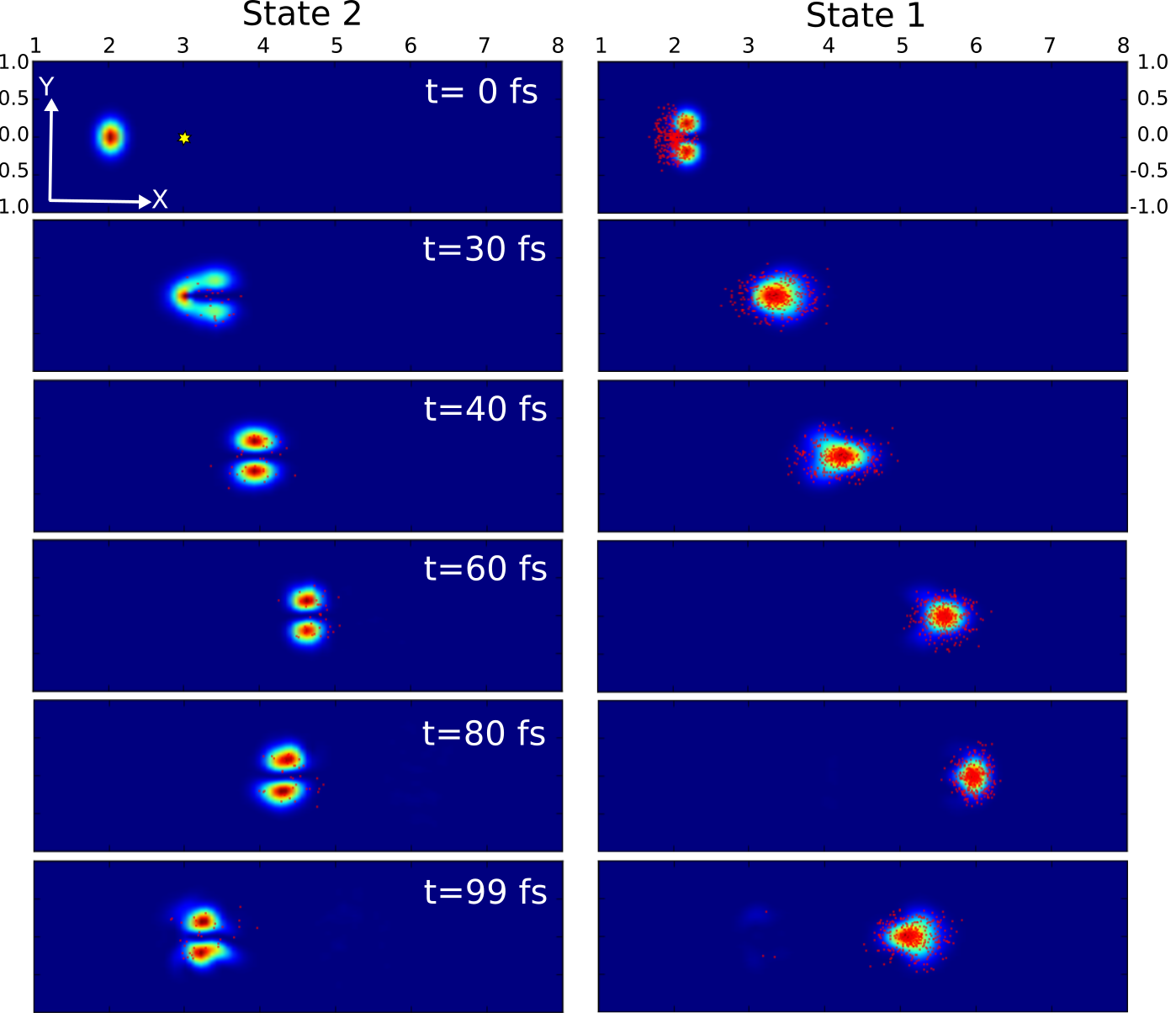
Figure 2: Adiabatic wave functions $|\Psi_{1,2}(X,Y,t)|^{2}$ for weak ($\gamma=0.01$) coupling at different times. The position of the CI is marked by a small yellow star in the first frame. The red dots indicate the centers of the coherent states, which guide the moving basis set. The wavepackets were transformed from the diabatic representation (in which the simulation is performed) to the adiabatic representation, while trajectories are shown for diabatic states. Therefore at time $t=0.0$ fs all red dots are located on the diabatic state 1, whereas the wavepacket starts out in the adiabatic state 2. For better contrast, the color range extends from $|\Psi_{1,2}|_{\text{min}}^{2}$ (blue) to $|\Psi_{1,2}|_{\text{max}}^{2}$ (red) in each image; at $t=0$ fs, $|\Psi_{2}(0)|_{\text{max}}^{2}=3.6$, $|\Psi_{1}(0)|_{\text{max}}^{2}=8\cdot 10^{-5}$ and at $t=99$ fs, $|\Psi_{2}(99)|_{\text{max}}^{2}=0.2$, $|\Psi_{1}(99)|_{\text{max}}^{2}=1.6$.

strong coupling ($\Gamma=0.08$):

To reproduce the numerically exact results, much more trajectories are needed for the strong coupling regime than for the weak one.

Initial conditions for 1500 trajectories are sampled from $W(q,p)^{1/3}$. Sampling from the cubic root of the Wigner distribution makes the initial trajectory distribution more diffuse, so that the trajectories do not overlap too much. A nuclear time step of $\Delta t_{\text{nuc}}=0.01$ fs and an electronic time step of $\Delta t_{\text{elec}}=3\cdot 10^{-6}$ was used. The resulting total state probabilities are shown in Fig.3, snapshots of the wavepacket evolution are shown in Fig.4.

Interestingly, most of the time is spent in integrating the electronic populations for the surface hopping procedure, so the cost of CCS dynamics is not so different from usual surface hopping. The limitation is that for CCS dynamics the potential energy surface has to be known globally (e.g. in the form of a force field) while for surface hopping local knowledge of the energy, gradient and non-adiabatic couplings is enough.

Figure 3: State probabilities for strong ($\Gamma=0.08$) coupling in the a) diabatic and b) adiabatic picture. Numerically exact (solid), CCS dynamics (dashed).

Figure 4: Adiabatic wave functions $|\Psi_{1,2}(X,Y,t)|^{2}$ for strong ($\gamma=0.08$) coupling at different times.

Trajectory Populations:

It is also instructive to look at the populations of the guiding trajectories on the two diabatic states (see Fig.5). In the case of weak coupling the trajectory populations underestimate the transfer of population between the diabatic states. In the case of strong coupling they look completely different: The initial conditions were sampled from the cubic root of the Wigner function, and therefore represent a different semiclassical wavepacket. Using a different initial distribution is a valid trick, since the trajectories only function as a basis, which can be distributed at will as long as it covers the region where the wavepacket passes through. The quantum populations still agree very well for both coupling strengths (see Figs. 1 and 3).

Figure 5: Comparison between trajectory populations and QM probabilities for a) weak and b) strong coupling. The trajectory populations (dots) are obtained by counting the number of trajectories on each diabatic state. In b) the trajectory populations deviate from the quantum populations, because the initial distribution were sampled not from the Wigner distribution $W(q,p)$ but from $W(q,p)^{1/3}$.

IV Conclusions and Outlook

By solving the Schr dinger equation in the basis of surface hopping coherent states the complex interference effects around a conical intersection can be fully reproduced. This is not surprising as no approximations have been made apart from using a finite basis set. Therefore, the method could serve as an alternative to numerically exact grid-based propagation schemes in more than 3 dimensions, provided the diabatic potentials can be expressed in a form, for which the matrix elements between coherent states can be computed analytically. This is a severe limitation that does not affect direct dynamics schemes, where only adiabatic gradients and non-adiabatic couplings are required. On the other hand, although methods for direct quantum dynamics are sometimes claimed to be exact, a convergence to the exact result is not guaranteed, if matrix elements are approximated for compatibility with electronic structure calculations.

Further work will focus on developing building blocks for analytical molecular potentials. Molecular diabatic potentials can be expanded into terms depending only on bond lengths, bond angles, dihedrals etc.; conical intersections or avoided crossing can be modelled by Gaussians placed on the off-diagonals. The averaging integrals would have to be worked out for a set of force field-like terms from which potential energy surfaces for larger molecules can be constructed in the spirit of empirical valence bond theorywarshel_evb ; ms_evb . This would allow to perform numerically exact quantum dynamics on model potentials to investigate the photochemistry of small molecules.

V Acknowledgements

We thank Stewart Reed for making his CCS code publicly available, which has proven helpful in debugging the code developed for this work. The financial support by the European Research Council (ERC) Consolidator Grant “DYNAMO” Grant Nr. is gratefully acknowledged.

Appendix A Appendix

A.1 Wavefunction in the CCS representation

The basis of surface hopping coherent states offers a very compact representation for a multi-dimensional wavefunction that can be delocalized over many electronic states. For convenience a few useful relations are list here:

• The wave function is the following superposition of the basis functions:

  $$\mid\Psi\rangle=\sum_{i}\mid\textbf{z}_{i},\mathbf{a}_{i}\rangle D_{i}e^{\frac{\text{\rm{i}}}{\hbar}S_{i}}$$ (45)

• Its norm is given by:

  $$\langle\Psi\mid\Psi\rangle=\sum_{i}C_{i}^{*}D_{i}$$ (46)

• The total energy, which in the absence of an external field should be a conserved quantity, is

  $$E_{\text{tot}}=\langle\Psi\mid\hat{H}\mid\Psi\rangle=\sum_{i}\left(D_{i}e^{\frac{\text{\rm{i}}}{\hbar}S_{i}}\right)^{*}\sum_{j}\langle\mathbf{z}_{i}\mid\mathbf{z}_{j}\rangle\left(\sum_{A,B}a_{i}^{A*}H_{AB}^{\text{ord}}\left(\mathbf{z}_{i}^{*},\mathbf{z}_{j}\right)a_{j}^{B}\right)\left(D_{j}e^{\frac{\text{\rm{i}}}{\hbar}S_{j}}\right),$$ (47)

• and the quantum probability to be on state $I$ can be obtained as:

  $$p_{I}=|\langle I\mid\Psi\rangle|^{2}=\sum_{i,j}\left(D_{i}a_{i}^{I}e^{\frac{\text{\rm{i}}}{\hbar}S_{i}}\right)^{*}\langle\mathbf{z}_{i}\mid\mathbf{z}_{j}\rangle\left(D_{j}a_{j}^{I}e^{\frac{\text{\rm{i}}}{\hbar}S_{j}}\right)$$ (48)

A.2 Guiding equations for a diabatic hamiltonian

For a diabatic hamiltonian with the form

$$\hat{H}_{AB}=\delta_{AB}T(\hat{\mathbf{p}})+V_{AB}(\mathbf{x})=\delta_{AB}\sum_{d=1}^{N_{\text{dim}}}\frac{\hat{p}_{d}^{2}}{2m_{d}}+V_{AB}(x_{1},\ldots,x_{d})$$ (49)

the kinetic energy can be reordered algebraically to give

$$T^{\text{ord}}(\mathbf{z}_{i}^{*},\mathbf{z}_{j})=-\frac{\gamma\hbar^{2}}{4}\sum_{d=1}^{N_{\text{dim}}}\frac{1}{m_{d}}\left[\left(z_{j,d}-z_{i,d}^{*}\right)^{2}-1\right].$$ (50)

with the gradient

$$\frac{\partial}{\partial z_{d}^{*}}T^{\text{ord}}(\mathbf{z},\mathbf{z})=\frac{\text{\rm{i}}\hbar^{2}\gamma}{m_{d}}\Im(z_{d})$$ (51)

The equations of motion for the action, the complex position vector and the electronic amplitudes of a trajectory become

$$\frac{dS}{dt} = =\sum_{d=1}^{N_{\text{dim}}}\frac{\hbar^{2}\gamma}{m_{d}}\left(\Im(z_{d})\right)^{2}+\Re(\mathbf{z})\cdot\frac{\partial V_{II}^{\text{ord}}}{\partial\mathbf{z}}$$ (52)

$$\frac{dz_{d}}{dt} = \frac{\hbar\gamma}{m_{d}}\Im(z_{d})-\frac{\text{\rm{i}}}{\hbar}\frac{\partial V_{II}^{\text{ord}}}{\partial z_{d}}$$ (53)

$$\frac{da^{A}}{dt} = -\frac{\text{\rm{i}}}{\hbar}\sum_{B}\left[T^{\text{ord}}(\mathbf{z}^{*},\mathbf{z})\delta_{AB}+V_{AB}^{\text{ord}}(\mathbf{z}^{*},\mathbf{z})\right]a^{B}$$ (54)

where $\Re$ and $\Im$ denote the real and imaginary part and $I$ is the current electronic state of the trajectory.

A.3 Interaction with light

Interaction with a time-dependent external electric field can be included to simulate pump-probe experiments or coherent control. For simplicity, the vectorial nature of the electric field is neglected, and the dot product between the field vector and the transition dipole, $\vec{E}\cdot\vec{\mu}$, is replaced by $E\mu$. The additional time-dependent part of the Hamiltonian reads:

$$\hat{H}_{AB}^{\text{field}}(t)=E(t)V_{AB}^{\text{field}}(\mathbf{x})$$ (55)

where $E(t)$ only depends on time and $V_{AB}^{\text{field}}(\mathbf{x})$ represents the magnitudes of the transition dipoles between the electronic states $A$ and $B$ (which depend on the nuclear geometries). Since the time-dependence is limited to $E(t)$, the integrals for “reordering” $V_{AB}^{\text{field}}$ have to be calculated only once every nuclear time-step and remain constant during the integration of the electronic amplitudes. The hopping probabilities of the coherent states are driven by the electric field as in the field-induced surface hopping (FISH) method Petric_hopping_probabilities . In Fig. 6 the quantum-populations of the electronic states in the $K_{2}$ molecule during excitation with a shaped pulse are shown.

Figure 6: Field induced dynamics in K₂. Analytical functions of the bond length were fitted to the diabatic potential energy surfaces and transition dipoles of K₂ at the CASSCF/MRCI levelPetric_hopping_probabilities . The wavepacket, initially prepared on the ground state, was propagated using 300 coherent state trajectories in the presence of a short light-pulse. Although the problem is effectively one-dimensional, the trajectories were propagated including all 6 cartesian coordinates. a) Time-dependence $E(t)$ of the electric pulse (same as in Fig 2a of Ref. Petric_hopping_probabilities ), b) Quantum populations obtained with surface hopping coherent states.

References

- (1) Doltsinis, N.; Marx, D.; First principles molecular dynamics involving excited states and non-adiabatic transitions. J. Theor. Comput. Chem., 2002, 1, 319-349.
- (2) Lobaugh, J.; Voth, G.; The quantum dynamics of an excess proton in water. J. Chem. Phys., 1996, 104, 2056-2069.
- (3) Mead, A.; Truhlar, D.; On the determination of Born-Oppenheimer nuclear motion wave functions including complications due to conical intersections and identical nuclei. J. Chem. Phys., 1979, 70, 5.
- (4) Conical Intersections: Electronic Structure, Dynamics and Spectroscopy, edited by Domcke, W.; Yarkony, D.; K ppel, H.; World Scientific Publishing, Singapore, 2004.
- (5) Yarkony, D.; Diabolic conical intersections. Rev. Mod. Phys., 1996, 68, 4.
- (6) Abe, M.; Ohtsuki, Y.; Fujimura, Y.; Lan, Zh.; Domcke, W.; Geometric phase effects in the coherent control of the branching ratio of photodissociation products of phenol. J. Chem. Phys., 2006, 124, 224316.
- (7) Shalashilin, D.; Child, M.; The phase CCS approach to quantum and semiclassical molecular dynamics for high-dimensional systems. Chem. Phys. 2004, 304, 103-120.
- (8) Heller, E.; Frozen Gaussians: A very simple semiclassical approximation. J. Chem. Phys., 1981, 75, 2923.
- (9) Shalashilin, D.; Nonadiabatic dynamics with the help of multiconfigurational Ehrenfest method: Improved theory and fully quantum 24D simulation of pyrazine. J. Chem. Phys. 2010, 132, 244111.
- (10) Tully, J.; Molecular dynamics with electronic transitions. J. Chem. Phys. 1990, 93, 1061.
- (11) Horenko, I.; Salzmann, Ch.; Schmidt, B.; Sch tte,Ch.; Quantum-classical Liouville approach to molecular dynamics: Surface hopping Gaussian phase-space packets. J. Chem. Phys., 2002, 117, 11075.
- (12) Meyer,H-D.; Gatti, F.; Worth,G.; Multdimensional Quantum Dynamics - MCTDH Theory and Applications. Wiley-VCH, 2009.
- (13) Vendrell, O.; Gatti, F.; Meyer, H-D.; Dynamics and Infrared Spectroscopy of the Protonated Water Dimer. Angew. Chem. Int. Ed., 2007, 46, 6918-6921.
- (14) Ben-Nun, M.; Martínez, T.; Ab initio quantum molecular dynamics. Adv. Chem. Phys. 2002, 121, 439.
- (15) Martínez, T.; Ab initio molecular dynamics around a conical intersection: Li(p)+H2. Chem. Phys. Lett., 1997, 272, 139-147.
- (16) Ben-Nun, M.; Martínez, T.; A multiple spawning approach to tunneling dynamics. J. Chem. Phys. 2000, 112, 6113.
- (17) Makhov, D.; Glover, W.; Martínez, T.; Shalashilin, D.; Ab initio multiple cloning algorithm for quantum non-adiabatic molecular dynamics. J. Chem. Phys. 2014, 141, 054110.
- (18) Heitz, M.; Durand, G.; Spiegelman, F.; Ultrafast excited state dynamics of the Na3F cluster: Quantum wave packet and classical trajectory calculations compared to experimental results. J. Chem. Phys., 2004, 121, 9906-9916.
- (19) Dixon, R.; A Three-dimensional Time-dependent Wavepacket Calculation for Bound and Quasi-bound Levels of the Ground State of HCO: Resonance Energies, Level Widths and CO Product State Distributions. J. Chem. Soc. Faraday Trans., 1992, 88, 2575-2586.
- (20) Reed, S.; Gonz lez Martínez, L.; Rubayo Soneira, J.; Shalashilin, D.; Cartesian coupled coherent states simulations: Ne n Br2 dissociation as a test case. J. Chem. Phys. 2011, 134, 054110.
- (21) Shalashilin, D.; Child, M.; Basis set sampling in the method of coupled coherent states: Coherent state swarms, trains and pancakes. J. Chem. Phys., 2007, 128, 054102.
- (22) Levine, B.; Coe, J.; Virshup, A.; Martínez, T.; Implementation of ab initio multiple spawning in the MOLPRO quantum chemistry package. J. Chem. Phys., 2008, 347, 3-16.
- (23) Worth, G.; Meyer, H.; K ppel, H.; Cederbaum, L.; Burghardt, I.; Using the MCTDH wavepacket propagation method to describe multimode non-adiabatic dynamics. Int. Rev. in Phys. Chem., 2008, 27, 569-606.
- (24) Worth, G.; Robb, M.; Burghardt, I.; A novel algorithm for non-adiabatic direct dynamics using variational Gaussian wavepackets. Faraday Discuss., 2004, 127, 307-323.
- (25) Nangia, Sh.; Truhlar, D. Direct calculation of coupled diabatic potential-energy surfaces for ammonia and mapping of a four-dimensional conical intersection seam. J. Chem. Phys., 2006, 124, 124309.
- (26) Klauder, J.; Skagerstam, B.; Coherent States - Applications in Physics and Mathematical Physics. World Scientific, 1985.
- (27) Anderson, E.; Bai,Z.; Bischof, C.; Blackford, S.; Demmel, J.; Dongarra, J.; Du Croz, J.; Greenbaum, A.; Hammarling, S.; McKenney, A.; Sorensen, D. LAPACK Users’ Guide. Society for Industrial and Applied Mathematics, 1999, 3rd edition.
- (28) Ferretti, A.; Granucci, G.; Lami, A.; Persico, M.; Villani, G. Quantum mechanical and semiclassical dynamics at a conical intersection. J. Chem. Phys., 1996, 104, 5517.
- (29) To appreciate intuitively why moving basis sets can be very efficient imagine a TV crew is to cover the Tour de France. If they would like to cover the entire sports event with stationary cameras, they would have to place a camera every few hundred meters along the entire route. Most of the camera would not see anything interesting for most of the time. If they mount cameras on cars and follow the peloton, relatively few cameras are needed depending on how closely the cyclists stay together.
- (30) Petersen, J.; Mitrić, R.; Electronic coherence within the semiclassical field-induced surface hopping method: strong field quantum control in . Phys. Chem. Chem. Phys. 2012, 14, 8299-8306.
- (31) Kosloff, D.; Kosloff, R. A Fourier Method Solution for the Time Dependent Schr dinger Equation as a Tool in Molecular Dynamics. J. Comput. Phys., 1983, 52, 35-53.
- (32) Warshel, A.; Weiss, R.; An Empirical Valence Bond Approach for Comparing Reactions in Solutions and in Enzymes. J. Am. Chem. Soc., 1980, 102, 6218-6226.
- (33) Schmitt, U.; Voth, G.; Multistate Empirical Valence Bond Model for Proton Transport in Water. J. Phys. Chem. B, 1998, 102, 29.