Internal dipolar field and soft magnons in periodic nanocomposite magnets

Abstract

We study spin wave excitations in a three-dimensional nanocomposite magnet of exchange coupled hard (SmCo₅) and soft (FeCo) phases. The dipolar interaction splits the spin wave energies into the upper and lower branches of the spin wave manifold. When the amount of the soft phase is increased the energy of low-lying spin excitations is considerably softened due to two reasons: (i) the low- lying mode locked into the soft phase region with a spin wave gap at ${\bf k}=0$ which scales approximately proportional to the anisotropy constant of the soft phase and (ii) the internal dipolar field which comes from magnetic charges forming at hard-soft boundaries with normals parallel to the magnetization displaces the spin wave manifold toward the lower energies. With adding more soft phase the spin wave gap closes and the system moves to another ground state characterized by the magnetization mismatch between spins of the hard and soft phases.

Keywords: nanocomposite magnets, spin waves, dipolar interaction, remanent magnetization

1 Introduction

Materials with periodically modulated magnetic and geometric properties are of special interest recently from the viewpoint of applications, which aim to manipulate propagating spin waves [1, 2, 3, 4, 5]. Spin waves propagating in nonhomogeneous magnetic nanostructures serve as information carriers and show the existence of allowed frequency ranges and forbidden band gaps [6, 7, 8, 9, 10, 11]. The periodic modulation of magnetic properties are also realized in nanocomposite magnets composed of exchange-coupled hard and soft magnetic phases [12, 13, 14]. The hard phase provides the immense magnetic anisotropy that stabilizes the exchange-coupled soft phase against demagnetization. In multilayer geometry it gives the increase in the remanent magnetization and the ultimate gain in the energy product with increasing amount of the soft phase material [15]. However, in a geometry where the nanocomposite is magnetized perpendicular to the hard-soft boundary, the anticipated increase in the remanence does not occur partly because the hard and soft phase magnetization vectors are never completely parallel to each other [16].

In a nonhomogeneous magnetic material values of the saturation magnetization $M_{S}$, anisotropy constant $K$ and the direction of the magnetization ${\bf n}_{0}$ are, in general, functions of the position vector ${\bf r}$. In a magnonic crystal the applied uniform magnetic field usually forces all the magnetic moments to be magnetized in the direction of the applied field [17, 18, 19]. In a nanocomposite hard-soft magnet the behavior of the magnetization vector ${\bf M}({\bf r})=M_{S}({\bf r}){\bf n}_{0}({\bf r})$ depends on the demagnetizing effects and mutual arrangement of easy axes of constituent ferromagnets. For an arrangement with easy axis (in the $z$ direction) perpendicular to the hard-soft boundary the homogeneously magnetized state ${\bf M}({\bf r})=M_{S}({\bf r}){\hat{z}}$ is energetically unfavorable from the magnetostatic point of view. Because of the discontinuity of the magnetization at the hard-soft boundary, a magnetic charge $\rho_{M}=-\nabla\cdot{\bf M}$ is developed. This increases the dipolar energy which can be written in the form [20] $E_{dip}\propto\int d^{3}rd^{3}r^{\prime}\rho_{M}({\bf r})\rho_{M}({\bf r^{\prime}})/|{\bf r}-{\bf r^{\prime}}|$. For sufficiently low soft phase content a strong anisotropy field of the hard phase and exchange forces at soft-hard boundaries enforce the whole magnet to be magnetized in the $z$ direction. With adding more soft phase with considerably smaller value of anisotropy constant the soft phase spins become tilted from the easy direction and their averaged direction are misaligned with spins of the hard phase. Monte Carlo simulation at finite temperatures [21] reveals that this misorientation grows with temperature and as the amount of the soft phase is increased. Such a misalignment, usually, is not considered in the context of magnonic crystals where the nonuniform static demagnetizing filed is assumed to be homogeneously averaged throughout the sample [17].

The dependence of the ground state magnetization in composite permanent magnets on the demagnetizing effects has been discussed previously for a single soft inclusion in a matrix of hard phase [22]. These calculations reveal that the remanent magnetization sensitively depends on the size of the inclusion. With increasing of the fraction of the soft phase the long-range stray field destroys the parallel alignment of the soft magnetic moments and creates magnetic vortex-like structures. These calculations are based on computational micromagnetism [23, 24, 25] and yield a stable magnetization distribution by minimizing the total energy of magnetic system.

Micromagnetic calculations [22] as well as an analytic estimate of the nucleation field and the remanence enhancement [15] have not discussed the thermally activated tilting of spins and the resulting magnetization mismatch. The effect of thermal activation can be understood if one knows the low-lying spin wave energies $E_{j}({\bf k})$. The fluctuation of the magnetization is determined by the density of the magnons which in turn is governed by the Boltzmann factor $\exp(-E_{j}({\bf k})/k_{B}T)$. The lower the energy of spin excitations, which turns out to be concentrated in the soft phase, the more fluctuations of the soft phase spins and more reduction in the remanent magnetization of the composite appears. Due to the fluctuation of soft phase spins the remanence does not increase proportional to the fraction of the soft phase, $M_{r}=v_{s}M_{s}+v_{h}M_{h}$ ($v_{s}+v_{h}=1$), as it can be for a composite with homogeneous magnetization.

To further elucidate the physics involved in the instability of the homogeneously magnetized state, ${\bf M}({\bf r})=M_{S}({\bf r})\hat{z}$, in the present work we consider the spin wave spectrum in a three-dimensional (3D) composite composed of a periodic array of hard phase cubes immersed into a soft phase matrix. We incorporate the effect of the nonhomogeneous saturation magnetization $M_{S}({\bf r})$ and internal magnetic chargers into the formalism of spin wave excitations. We explicitly construct operators of spin-wave excitations and calculate the corresponding eigenfrequencies. We anticipate that the dipolar interaction will lower the spin wave energy, which in turn enhances the fluctuation of the magnetization at finite temperatures as these spin waves are thermally excited.

A brief analysis of the spin wave spectra in a hard-soft composite was reported earlier in Ref. [26] for the case of homogeneous exchange interaction, $J_{ij}=const$ for any nearest neighbors $i$ and $j$, which does not include the discontinuity of $J_{ij}$ at hard-soft boundary. That study was focused on the comparison of the behavior of low-lying spin excitations with our previous Monte Carlo simulation results [16]. In this paper we extend our previous analysis of homogeneous exchange interaction [26] for the case of position-dependent exchange interaction $J({\bf R}_{i},{\bf R}_{j}$) and present the clarifying details of incorporating the dipolar part of interaction into the formalism of spin-wave excitations for nonhomogeneous ferromagnets. The main purpose of the work is to extract the effective demagnetizing field $H_{dip}$ from the spin-wave dispersion behavior and discuss the implication of $H_{dip}$ for spin-wave manifolds in two-phase and one-phase ferromagnets.

The paper is organized as follows. In Section II we present the general theory of linear spin-waves in a nonhomogeneous two-phase periodic structure of exchange-coupled hard and soft phases. We first linearize the spin Hamiltonian in the position space and then perform the diagonalization in the Fourier space. We then proceed in comparing the analytical results obtained for the behavior of low-lying spin excitations in a nonhomogeneous composite with the spin-wave spectra for homogeneous ferromagnets. In Sec. III we discuss results of our calculation and the effect of the internal demagnetizing field on the spin wave dispersion of the two-phase magnet. And Sec. IV contains our conclusion.

2 Theoretical model

2.1 Two-phase composite magnet

We model the hard-soft composite as a periodic array of identical cubes of hard phase embedded into a soft phase matrix, as illustrated in Fig. 1. The easy axes of both phases are in the $z$ direction. Each cube has a linear dimension $l_{h}$ and separated from the adjacent one by a soft phase with linear dimension $l_{s}$, so there is a periodicity in the $x$, $y$ and $z$ directions with a period $w=l_{h}+l_{s}$. We shall refer to this periodicity as $w$- periodicity.

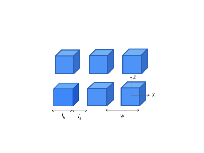
Figure 1: Geometry of hard-soft periodic structure. The $z$ axis is the easy axis for the hard and soft phases.

We focus on the low-lying spin excitations that occur gradually over a large distance. The magnetization, ${\bf M}({\bf r})$, for a coarse-grained system, is defined on a discrete set of sites ${\bf R}_{i}$ in terms of block spin variables ${\bf S}_{i}=~{}{\bf S}({\bf R}_{i})$, $|{\bf S}_{i}|=~{}1$, as ${\bf M}({\bf r})\simeq M({\bf R}_{i}){\bf S}_{i}$, with $M({\bf R}_{i})=M_{S}({\bf R}_{i})$ being the saturation magnetization density of the hard ($M_{h}$) or soft ($M_{s}$) phase at site $i$. Spins of the hard and soft phases are arranged in a three-dimensional cubic lattice with an effective lattice constant $a$. The effective magnetic moment of site $i$ is $M({\bf R}_{i})v$, where $v=a^{3}$ is the volume of a block spin cell.

The interaction between two spins ${\bf S}_{i}$, ${\bf S}_{j}$ located at ${\bf R}_{i}$, ${\bf R}_{j}$ is described by the Hamiltonian for a classical spin system, including the nearest-neighbor exchange energy, the uniaxial magnetic anisotropy term and the dipole-dipole interaction:

$$H=-\frac{1}{2}{\,}\mathop{{\sum}^{\prime}}_{i,j}{\,}J_{ij}{\,}{\bf S}_{i}\cdot{\bf S}_{j}-\sum\limits_{i}{\;}K_{i}{\,}\left(S^{z}_{i}\right)^{2}-\frac{g}{2}{\,}\mathop{{\sum}^{\prime}}_{i,j}{\,}D^{\alpha\beta}({\bf R}_{ij})M({\bf R}_{i})M({\bf R}_{j}){\,}S^{\alpha}_{i}S^{\beta}_{j},$$ (1)

where ${\bf R}_{ij}={\bf R}_{i}-{\bf R}_{j}$, and the summations are over all distinct magnetic sites $i$ and $j$ with the restriction that ${\bf R}_{ij}\neq 0$. Indices $\alpha$ and $\beta$ denote the Cartesian components $x$, $y$ or $z$, and $D^{\alpha\beta}({\bf R}_{ij})=(3R^{\alpha}_{ij}R^{\beta}_{ij}-R^{2}_{ij}\delta_{\alpha\beta})/R^{5}_{ij}$ is the dipolar interaction tensor. In Eq. (1) positions vectors ${\bf R}_{i}$ are given in units of the lattice spacing $a$. The exchange constant $J_{ij}$, is equal to $J_{h}$ ($J_{s}$) for the nearest neighbor spins of hard (soft) phase and zero otherwise. The two phases are exchange-coupled with a coupling constant $J_{hs}$ which can be estimated as the geometric mean of $J_{h}$ and $J_{s}$, $J_{hs}=(J_{h}J_{s})^{1/2}$. $K_{i}$ is the anisotropy constant of the hard ($K_{h}$) or soft ($K_{s}$) phase. The characteristic magnetostatic energies of the hard and soft phases are $g_{h}=\mu_{0}M_{h}^{2}v/(4\pi)$ and $g_{s}=\mu_{0}M_{s}^{2}v/(4\pi)$, respectively. In Eq. (1) we assume that the magnetization density $M({\bf R}_{i})$ is normalized by the magnetization of the hard phase $M_{h}$, and the dipolar coupling constant $g$ is equal to $g_{h}$.

We use the Holstein-Primakoff transformation [27] to express the spin operators through the boson creation and annihilation operators, $a^{\dagger}_{i}$, $a_{i}$, as $S^{+}_{i}\simeq\sqrt{2S}{\,}a_{i}$, $S^{-}_{i}\simeq\sqrt{2S}{\,}a^{\dagger}_{i}$, and $S^{z}_{i}\simeq S-a^{\dagger}_{i}a_{i}$. We assume that the ground state is the one with all spins of both phases aligned along the $z$ direction and expand near this aligned state.

In the harmonic approximation we can rewrite the spin Hamiltonian as

$$H=\mathop{{\sum}^{\prime}}_{i,j}{\,}J_{ij}\left[a^{\dagger}_{i}a_{i}-a^{\dagger}_{i}a_{j}\right]+\sum\limits_{i}{\,}2K_{i}a^{\dagger}_{i}a_{i}+g\mathop{{\sum}^{\prime}}_{i,j}{\,}M({\bf R}_{i})M({\bf R}_{j})\times$$

$$\times\left\{A_{1}({\bf R}_{ij})a^{\dagger}_{i}a_{j}+A_{2}({\bf R}_{ij})a^{\dagger}_{i}a_{i}+\frac{1}{2}B({\bf R}_{ij})a_{i}a_{j}+\frac{1}{2}B^{*}({\bf R}_{ij})a^{\dagger}_{i}a^{\dagger}_{j}\right\},$$ (2)

where coefficients $A_{1,2}({\bf R}_{ij})$ and $B({\bf R}_{ij})$ are

$$A_{1}({\bf R}_{ij})=\frac{1}{2}D^{zz}({\bf R}_{ij});\qquad A_{2}({\bf R}_{ij})=D^{zz}({\bf R}_{ij}),$$ (3)

$$B({\bf R}_{ij})=(-1/2)\left[D^{xx}({\bf R}_{ij})-D^{yy}({\bf R}_{ij})-2iD^{xy}({\bf R}_{ij})\right].$$ (4)

Diagonalizing the spin-wave Hamiltonian, Eq. (2.1), can be performed in usual way transforming to new quasiparticle boson operators $\alpha_{l},\alpha_{l}^{\dagger}$, $l=1,\dots,N$, with $N$ being the number of lattice sites, and using the $u-v$ Bogoliubov transformation

$$\eqalign{a_{i}=\sum\limits_{l}{\,}\left\{u_{l}({\bf R}_{i})\alpha_{l}-v^{*}_{l}({\bf R}_{i})\alpha^{\dagger}_{l}\right\},\\ a_{i}^{\dagger}=\sum\limits_{l}{\,}\left\{u^{*}_{l}({\bf R}_{i})\alpha_{l}^{\dagger}-v_{l}({\bf R}_{i})\alpha_{l}\right\}.}$$ (5)

The coefficients of the transformation $u({\bf R}_{i})$ and $v({\bf R}_{i})$ can be found from the equation of motion for operators $a_{i}$ and $\alpha_{l}$, provided that $\alpha_{l}$ corresponds to the eigenmode of the system, $i\hbar\dot{\alpha}_{l}=E_{l}\alpha_{l}$. From this we obtain the following system of equations

$$2K_{i}u({\bf R}_{i})+\sum\limits_{j\neq i}\Bigl{\{}\Bigl{(}gA_{1}({\bf R}_{ij})M({\bf R}_{i})M({\bf R}_{j})-J_{ij}\Bigr{)}u({\bf R}_{j})$$

$$+\Bigl{(}gA_{2}({\bf R}_{ij})M({\bf R}_{i})M({\bf R}_{j})+J_{ij}\Bigr{)}u({\bf R}_{i})-B^{*}({\bf R}_{ij})M({\bf R}_{i})M({\bf R}_{j})v({\bf R}_{j})\Bigr{\}}=E_{l}u({\bf R}_{i}),$$ (6)

$$-2K_{i}v({\bf R}_{i})+\sum\limits_{j\neq i}\Bigl{\{}-\Bigl{(}gA_{1}({\bf R}_{ij})M({\bf R}_{i})M({\bf R}_{j})-J_{ij}\Bigr{)}v({\bf R}_{j})$$

$$-\Bigl{(}gA_{2}({\bf R}_{ij})M({\bf R}_{i})M({\bf R}_{j})+J_{ij}\Bigr{)}v({\bf R}_{i})+B({\bf R}_{ij})M({\bf R}_{i})M({\bf R}_{j})u({\bf R}_{j})\Bigr{\}}=E_{l}v({\bf R}_{i}).$$ (7)

To proceed further we expand the eigenmode functions $u({\bf R})$ and $v({\bf R})$ into a series on a full set of functions $\{\varphi_{l}({\bf R}_{i})\}$

$$\eqalign{u({\bf R}_{i})=\sum\limits_{l^{\prime}}u_{l^{\prime}}{\,}\varphi_{l^{\prime}}({\bf R}_{i}),\\ v({\bf R}_{i})=\sum\limits_{l^{\prime}}v_{l^{\prime}}{\,}\varphi_{l^{\prime}}({\bf R}_{i}).}$$ (8)

The corresponding coefficients of the expansion $u_{l}$ and $v_{l}$ can be found from the following system of $2N$ coupled equations

$$\left\{\begin{array}[]{rcl}A_{ll^{\prime}}u_{l^{\prime}}-B^{\dagger}_{ll^{\prime}}v_{l^{\prime}}&=&E_{l}u_{l},\\ B_{ll^{\prime}}u_{l^{\prime}}-A_{ll^{\prime}}v_{l^{\prime}}&=&E_{l}u_{l}\end{array}\right.$$ (9)

where summation is implied over the repeated index. This can be conveniently rewritten in the block matrix form as

$$\left(\begin{array}[]{cc}A&-B^{\dagger}\\ B&-A\end{array}\right)\left(\begin{array}[]{c}u\\ v\end{array}\right)=E\left(\begin{array}[]{c}u\\ v\end{array}\right),$$ (10)

where vector $\left(u\atop v\right)$ has components $(u_{1},\dots,u_{N},v_{1},\dots,v_{N})^{T}$ and $A$ and $B$ are N-by-N matrices with the following matrix elements

$$A_{ll^{\prime}}=\sum\limits_{i}{\,}\varphi^{*}_{l}({\bf R}_{i}){\,}2K_{i}{\,}\varphi_{l^{\prime}}({\bf R}_{i})+\mathop{{\sum}^{\prime}}_{i,j}{\,}\varphi^{*}_{l}({\bf R}_{i})\Bigl{(}gA_{1}({\bf R}_{ij})M({\bf R}_{i})M({\bf R}_{j})-J_{ij}\Bigr{)}\varphi_{l^{\prime}}({\bf R}_{j})$$

$$+\mathop{{\sum}^{\prime}}_{i,j}{\,}\varphi^{*}_{l}({\bf R}_{i})\Bigl{(}gA_{2}({\bf R}_{ij})M({\bf R}_{i})M({\bf R}_{j})+J_{ij}\Bigr{)}\varphi_{l^{\prime}}({\bf R}_{i}),$$ (11)

$$\eqalign{B_{ll^{\prime}}=\mathop{{\sum}^{\prime}}_{i,j}{\,}\varphi^{*}_{l}({\bf R}_{i})B({\bf R}_{ij})M({\bf R}_{i})M({\bf R}_{j})\varphi_{l^{\prime}}({\bf R}_{i}),\\ B^{\dagger}_{ll^{\prime}}=\mathop{{\sum}^{\prime}}_{i,j}{\,}\varphi^{*}_{l}({\bf R}_{i})B^{*}({\bf R}_{ij})M({\bf R}_{i})M({\bf R}_{j})\varphi_{l^{\prime}}({\bf R}_{i})}$$ (12)

Matrices ${\cal L}=\left(\begin{array}[]{cc}A&-B^{\dagger}\\ B&-A\end{array}\right)$ and ${\cal L^{\prime}}=\left(\begin{array}[]{cc}A&B\\ -B^{\dagger}&-A\end{array}\right)$ can be transformed into each other by replacing $x$ with $y$. Such a substitution formally replaces $B$ with $-B^{\dagger}$ and vise versa. Because the spectrum $E$ is invariant under such a replacement, matrices ${\cal L}$ and ${\cal L^{\prime}}$ should have the same eigenvalues. From the other hand the similarity transformation, $S^{-1}{\cal L}S$ with a matrix $S=\left(\begin{array}[]{cc}0&-I\\ I&0\end{array}\right)$, transforms ${\cal L}$ into $-{\cal L^{\prime}}$. Thus, the eigenvalues of ${\cal L}$ should come up with pairs $E$ and $-E$.

The number of equations to solve can be substantially reduced if we use the $w$- periodicity and choose as a full set of function $\varphi_{\bf k}({\bf R}_{i})=1/\sqrt{N}\exp(i{\bf kR}_{i})$. Then the system of $2N$ coupled equations (10), with $N$ being the number of sites of the original cubic lattice, is reduced to $2N^{\prime}$ equation, with $N^{\prime}=(w/a)^{3}$ being the number of sites within one $w$ period. The corresponding Brillouin zone associated with $w$- periodicity has its boundaries at $\pm\pi/w$ and reciprocal vectors ${\bf G}=2\pi/w(l_{x},l_{y},l_{z})$, where $l_{x}$, $l_{y}$ and $l_{z}$ are integers. At a fixed ${\bf k}$ the operators (2.1) and (12) mix states ${\bf k}$ and ${\bf k+G}$ which can differ at most by one reciprocal vector. Number of different reciprocal vectors in the domain $|{\bf G}|\leqslant 2\pi/a$ is $N^{\prime}=(w/a)^{3}$. The $2N\times 2N$ matrix ${\cal L}$ is now divided into sub-blocks of a lower size $2N^{\prime}\times 2N^{\prime}$

$${\cal L}=\left(\begin{array}[]{cccc}{\cal L}({\bf k}_{1})&&&\\ &{\cal L}({\bf k}_{2})&&\\ &&\ddots&\end{array}\right)$$ (13)

Each sub-block ${\cal L}({\bf k})=\left(\begin{array}[]{cc}A_{pt}({\bf k})&-B^{\dagger}_{pt}({\bf k})\\ B_{pt}({\bf k})&-A_{pt}({\bf k})\end{array}\right)$ is labelled by a wave number ${\bf k}$, which runs over the first Brillouin zone. The corresponding sub-block equation has the form

$$\left(\begin{array}[]{cc}A_{pt}&-B^{\dagger}_{pt}\\ B_{pt}&-A_{pt}\end{array}\right)\left(\begin{array}[]{c}u_{t}\\ v_{t}\end{array}\right)=E\left(\begin{array}[]{c}u_{p}\\ v_{p}\end{array}\right)$$ (14)

where we use the short-hand notation for matrix elements $A_{pt}=A_{{\bf G}_{p}{\bf G}_{t}}({\bf k})$ and eigenvectors $\left(u_{t}\atop v_{t}\right)=(u_{G_{1}}({\bf k}),\dots,u_{G_{N^{\prime}}}({\bf k}),v_{G_{1}}({\bf k}),\dots,v_{G_{N^{\prime}}}({\bf k}))^{T}$. In Eq. (14) the sum is carried out over all reciprocal lattice vectors ${\bf G}_{t}$. The coefficients $A_{pt}$ and $B_{pt}({\bf k})$ containing contributions from the anisotropy, exchange and dipolar terms of the Hamiltonian (1) are given by

$$A_{pt}({\bf k})=2K_{\bf G_{p}-G_{t}}+\sum\limits_{\bf G}\widetilde{J}_{\bf G}\widetilde{J}_{\bf G_{p}-G_{t}-G}\left(F({\bf G})-F({\bf k+G_{p}-G})\right)$$

$$+g\sum\limits_{\bf G}\bigl{(}A_{1}({\bf k-G})+A_{2}({\bf G_{t}+G})\bigr{)}M_{\bf G_{p}+G}M^{*}_{\bf G_{t}+G}$$ (15)

$$\eqalign{B_{pt}({\bf k})=g\sum\limits_{\bf G}B({\bf k-G})M_{\bf G_{p}+G}M^{*}_{\bf G_{t}+G},\\ B^{\dagger}_{pt}({\bf k})=g\sum\limits_{\bf G}B^{*}({\bf k-G})M_{\bf G_{p}+G}M^{*}_{\bf G_{t}+G}.}$$ (16)

Here $M_{\bf G}$ and $K_{\bf G}$ are Fourier coefficients of the magnetization, $M({\bf R}_{i})=\sum\limits_{\bf G}M_{\bf G}e^{i{\bf GR}_{i}}$, and anisotropy, $K({\bf R}_{i})=\sum\limits_{\bf G}K_{\bf G}e^{i{\bf GR}_{i}}$, respectively. The Fourier transform of exchange interaction $J_{ij}$ is given in terms of $F({\bf k})=2(\cos(k_{x}a)+\cos(k_{y}a)+\cos(k_{z}a))$ and the Fourier transform $\widetilde{J}_{\bf k}$ of an auxiliary function $\widetilde{J}({\bf R}_{i})$ which is equal to $J_{h}^{1/2}$ in the hard phase and $J_{s}^{1/2}$ in the soft phase. The exchange coupling can be given in terms of $\widetilde{J}({\bf R}_{i})$ as $J_{ij}=\sum\limits_{\bf a}\widetilde{J}({\bf R}_{i})\widetilde{J}({\bf R}_{j})\delta_{{\bf R}_{i},{\bf R}_{j}+{\bf a}}$, where the summation is over nearest neighbors.

The lattice sums $A_{1,2}({\bf k})=\mathop{{\sum}^{\prime}}_{{\bf R}_{j}}{\>}e^{i{\bf k}{\bf R}_{ij}}A_{1,2}({\bf R}_{ij})$ and $B({\bf k})=\mathop{{\sum}^{\prime}}_{{\bf R}_{j}}{\>}e^{i{\bf k}{\bf R}_{ij}}B({\bf R}_{ij})$ can be presented in terms of the dipolar sum $D^{\alpha\beta}({\bf k})$ as follows, $A_{1}({\bf k})=D^{zz}({\bf k})/2$, $A_{2}({\bf G})=D^{zz}({\bf G})$ and $B({\bf k})=(-1/2)\left(D^{xx}({\bf k})-D^{yy}({\bf k})-2iD^{xy}({\bf k})\right)$. The dipole sum $D^{\alpha\beta}({\bf k})$ is defined by

$$D^{\alpha\beta}({\bf k})=\mathop{{\sum}^{\prime}}_{{\bf R}_{j}}{\>}e^{i{\bf k}{\bf R}_{ij}}D^{\alpha\beta}({\bf R}_{ij})$$ (17)

To determine $D^{\alpha\beta}({\bf k})$ we use the Ewald summation method [28, 29]. As is known the tensor $D^{\alpha\beta}({\bf k})$ is well- defined everywhere except point ${\bf k}=0$ [28, 29]. Further we treat the point ${\bf k}\to 0$ as the corresponding limit of $D^{\alpha\beta}({\bf k})$. This limit depends on the direction of vector ${\bf k}$ and gives rise to the dependence of the spin wave spectrum $E_{\bf k}$ on the direction of ${\bf k}$. The $D^{\alpha\beta}(0)$ occurs only in one term, $A_{2}({\bf G})$. The value of $D^{\alpha\beta}(0)$ is shape dependent and connected with the demagnetizing field of the homogeneously magnetized ellipsoidal-shaped magnetic body [30], $D^{\alpha\beta}(0)=-4\pi N_{{\alpha}{\beta}}+4\pi/3{\,}\delta_{\alpha\beta}$. The magnetic charges forming on the outer surface of the homogeneously magnetized finite body induce the demagnetizing field $H^{\alpha}_{dip}=-N_{\alpha\beta}M^{\beta}_{S}$.

Here we are interested in intrinsic properties of ferromagnetic media not affected by the presence of magnetic charges forming on the outer boundary. For infinitely extended system the demagnetizing tensor is $N_{{\alpha}{\beta}}=0$ [27, 31] and $D^{\alpha\beta}(0)=(4\pi/3){\,}\delta_{\alpha\beta}$. Earlier, to be consistent with the procedure of Monte Carlo simulation for a system with periodic boundary conditions we used $D^{\alpha\beta}(0)=0$ [26]. In a homogeneous ferromagnetic media it would result in a downward shift of the spin wave spectrum relative to the spectrum of a ferromagnet free of the dipolar interaction.

The structure of the system of equations (14) is similar to the coupled Bogoliubov equations for bosonic excitations in the theory of a Bose condensate [32]. The solution of the system of Eq. (14) yields in general a set of eigenfrequencies $E_{j}({\bf k})$ and eigenvectors $u_{tj}({\bf k}),v_{tj}({\bf k})$ labelled by a zone index $j$. For real eigenvalues $E_{j}$ the corresponding eigenfunctions are normalized by the condition [32]

$$\sum\limits_{t}\left(u_{tj^{\prime}}^{*}({\bf k})u_{tj}({\bf k})-v_{tj^{\prime}}^{*}({\bf k})v_{tj}({\bf k})\right)=\delta_{jj^{\prime}}.$$ (18)

The spatial profile of these eigenvectors for a magnon with momentum ${\bf k}$ and zone index $j$ can be visualized with the help of magnon wave functions $u_{{\bf k}j}({\bf R}_{i})$ and $v_{{\bf k}j}({\bf R}_{i})$, which can be found as follows:

$$\eqalign{u_{{\bf k}j}({\bf R}_{i})=\frac{1}{\sqrt{N^{\prime}}}\sum\limits_{{\bf G}_{t}}e^{i{\bf G}_{t}{\bf R}_{i}}u_{tj}({\bf k}),\\ v_{{\bf k}j}({\bf R}_{i})=\frac{1}{\sqrt{N^{\prime}}}\sum\limits_{{\bf G}_{t}}e^{i{\bf G}_{t}{\bf R}_{i}}v_{tj}({\bf k}).}$$ (19)

They are normalized by the condition which is followed from Eq. (18)

$$\sum\limits_{{\bf R}}\left(|u_{{\bf k}j}({\bf R})|^{2}-|v_{{\bf k}j}({\bf R})|^{2}\right)=1,$$ (20)

where the summation is over one $w$- period.

2.2 One-phase magnet

The magnetostatic interaction modifies the spectrum of exchange spin waves in two subtle ways. The first one is the dependence of $E_{\bf k}$ on the direction of ${\bf k}$, which gives rise to the notion of the spin wave manifold [33]. The second one is the dependence of $E_{\bf k}$ on the shape of the magnetic body, it comes from the long-range nature of magnetostatic forces. Before considering the effects of the magnetostatic interaction on the spin wave spectrum of a composite, we briefly illustrate the behavior of eigenfrequencies $E_{j}({\bf k})$ in a one-phase magnet for comparison. It will serve as a basis for our discussion of the spectrum for a two-phase magnet.

For the homogeneous one-component ferromagnet we can formally put $w=a$ and there is only one reciprocal vector ${\bf G_{p}}={\bf G_{t}}=0$ needs to be considered. In this case the system of equations (14) reduces to two equations for amplitudes $u_{\bf k}$ and $v_{\bf k}$ of the corresponding $u-v$ transformation. Accordingly, the corresponding coefficients $A_{pt}({\bf k})$ and $B_{pt}({\bf k})$ reduced to coefficients $A_{\bf k}$ and $B_{\bf k}$ of the Hamiltonian (21) given below.

Spin waves in homogeneous ferromagnet is a well-studied problem [27, 30, 34]. In the harmonic approximation the spin system Hamiltonian reads

$$H=\sum\limits_{\bf k}{\,}\left\{(\varepsilon_{\bf k}+gA_{\bf k})a^{\dagger}_{\bf k}a_{\bf k}+\frac{1}{2}gB_{\bf k}a_{\bf k}a_{\bf k}+\frac{1}{2}gB^{*}_{\bf k}a^{\dagger}_{\bf k}a^{\dagger}_{\bf k}\right\},$$ (21)

where $\varepsilon_{\bf k}=2K+6J(1-\gamma_{\bf k})$ is the spectrum of the ferromagnet without the dipole-dipole interaction term, $\gamma_{\bf k}=(1/3)(\cos(k_{x}a)+\cos(k_{y}a)+\cos(k_{z}a))$, $A_{\bf k}=D^{zz}({\bf k})/2+D^{zz}(0)$, $D^{zz}(0)=\mathop{{\sum}^{\prime}}_{{\bf R}_{j}}{\>}D^{zz}({\bf R}_{j})$ and $B_{\bf k}$ coincides with $B({\bf k})$ given above. For the case of infinitely extended ferromagnetic body when there is no demagnetizing field coming from the boundary magnetic charges the value of $D^{zz}(0)=4\pi/3$.

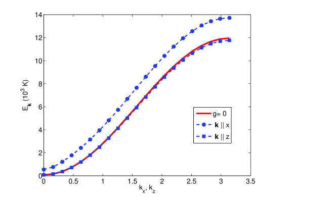
Figure 2: Spin wave excitations energies for the soft phase FeCo. The spectrum (dashed lines) is split into the upper and lower branches, corresponding to wave vectors parallel to the $x$ and $z$ direction, respectively. The spectrum of the ferromagnet $\varepsilon_{\bf k}$ without dipolar interaction ($g=0$) is shown by solid line.

The eigenvalues of the Hamiltonian (21) is well known [27, 30, 34]

$$E_{\bf k}=\sqrt{(\varepsilon_{\bf k}+gA_{\bf k})^{2}-g^{2}|B_{\bf k}|^{2}}$$ (22)

They corresponds to spin waves with momentum ${\bf k}$ propagating in infinitely extended magnetic body. For finite body this formula holds true for $k\gg 1/L$, where $L$ is the size the magnetic body. For this case $D^{zz}(0)=-4\pi N_{3}+4\pi/3$ also accounts for the demagnetizing field $H_{dip}=-N_{3}M_{S}$. The regions $k\lesssim 1/L$, corresponds to magnetostatic spin wave limit [35]. The spectrum of these modes depends on the boundary conditions of the magnetic body. We do not consider the magnetostatic modes, and treat the point ${\bf k}\to 0$ as the corresponding limit for the spin wave spectrum in an infinitely extended magnetic sample.

We illustrate the dispersion relation (22) in Fig. 2 for the soft phase FeCo. We considered the case of infinite media and thus $N_{3}=0$ and $H_{dip}=0$. Resulting spin wave excitations lie within the spin wave manifold $E_{\bf k}$. The upper and the lower branches of the manifold correspond to the wave vectors directed along $x$ and $z$ axes, respectively. The solid line presents the spectrum $\varepsilon_{\bf k}$, which does not account for the dipolar interaction. In the long wave limit, $ka\ll 1$, the lower branch of the manifold $E_{\bf k}$ coincides with the spectrum of pure exchange spin waves $\varepsilon_{\bf k}=2K+D{\bf k}^{2}$, $D=Ja^{2}$ is exchange stiffness.

3 Results and discussion

We illustrate our numerical calculation for a hard- soft composite SmCo₅/FeCo with the following parameters [36]: $K_{s}/k_{B}=40$ K, $J_{s}/k_{B}=2.9\cdot 10^{3}$ K, $\mu_{0}M_{s}=2.4$ T and $g_{s}/k_{B}=\mu_{0}M_{s}^{2}v/(4\pi k_{B})=290$ K for the soft phase FeCo; $K_{h}/k_{B}=13.3\cdot 10^{3}$ K, $J_{h}/k_{B}=3.3\cdot 10^{3}$ K, $\mu_{0}M_{h}=1.08$ T and $g_{h}/k_{B}=\mu_{0}M_{h}^{2}v/(4\pi k_{B})=57$ K for the hard phase SmCo₅, $k_{B}$ is the Boltzmann constant. The effective lattice constant is $a=2.2$ nm and is smaller than the magnetic length of the hard phase $l_{m,h}=\pi(A_{h}a^{3}/K)^{1/2}\simeq 2.5$ nm, $A_{h}$ is the exchange stiffness of the hard phase. Calculation were performed for hard-soft periodicity $w/a=20$. Further it is convenient to rescale $E_{j}({\bf k})$ by a factor of $k^{-1}_{B}$, so it is given in units of K. The linear dimensions of the hard (soft) phase $l_{h}$ ($l_{s}$) will be given in units of the cell size $a$ and the wave vector $k$ is rescaled via $ka$.

An example of the spin wave spectrum for the lowest magnon zone resulting from numerical solution of eigenproblem (14) is shown in Fig. 3. Four panels of Fig. 3 show the evolution of the spectrum with increasing soft phase content $l_{s}$. The solid line presents the spin wave spectrum $\varepsilon_{\bf k}$ obtained without the dipole-dipole interaction term ($g=0$). As expected the spin wave energies depend on direction of the wave vector ${\bf k}$ forming the spin-wave manifold. The lowest and the upper branches of the spectrum correspond to the spin waves propagating parallel to the $z$ and $x$ direction, respectively. The splitting is of order of the characteristic magnetostatic energy of the soft phase $g_{s}\simeq 300K$. With adding more soft phase the spin wave manifold gradually displaces downward relative to $\varepsilon_{\bf k}$. This can be attributed to the existence of the nonzero effective demagnetizing field due to the magnetic non-homogeneity. This is qualitatively different from the spectrum shown at Fig. 2, with the lower branch of $E_{\bf k}$ matching $\varepsilon_{\bf k}$. Eventually with increasing the soft phase amount the spin wave manifold presented in Fig. 3 touches $E_{\bf k}=0$ signalling that the homogeneously magnetized state is no longer the ground state of the periodic array of hard phase cubes immersed into the soft phase matrix. In this respect $E_{\bf k}=0$ cannot gradually evolves into the manifold presented in Fig. 2 with increasing the soft phase amount.

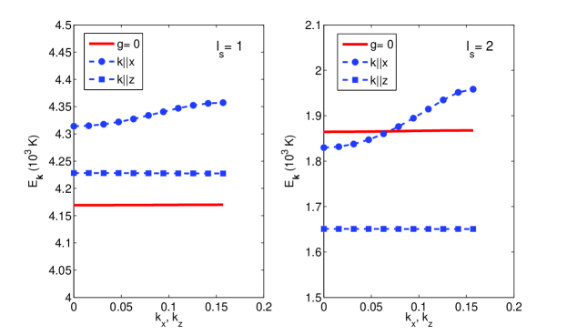
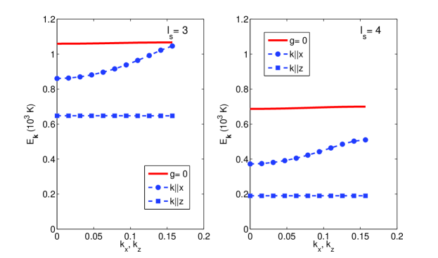
Figure 3: The spin wave spectrum evolution with increasing soft phase content from $l_{s}=1$ to $l_{s}=4$. The solid line ($g=0$) represents result for the spectrum $\varepsilon_{\bf k}$ without the dipole- dipole interaction. Lines with markers represent the lower and upper branches of the spin wave spectrum.

The corresponding magnon wave functions $u_{\bf k}({\bf R})$ and $v_{\bf k}({\bf R})$, both for the upper and the lower branches of $E_{\bf k}$, show the maximum magnitude in the soft phase and are strongly suppressed in the hard phase, i.e. the low-lying spin excitations are mostly concentrated into the soft phase. In our earlier work [26] we considered the hard-soft composite SmFeN/FeCo with homogeneous exchange interaction $J_{ij}=J$. We found the the similar behavior of magnon wave functions and the excitation spectrum $E_{\bf k}$ with increasing the soft phase content. It indicates that the discontinuity of exchange constant $J_{ij}$ on hard-soft boundaries is not crucial for the aforementioned lowering of $E_{\bf k}$ with increasing $l_{s}$. The situation closely parallels that studied in Ref. [17] for three-dimensional periodic structure of two different soft ferromagnetic materials. They found that the magnonic gap in spin wave dispersion is controlled by the variation of the spontaneous magnetization contrast between two phases.

The fluctuation of the magnetization is determined by the density of the magnons which in turn is governed by the Boltzmann factor $\exp(-E_{j}({\bf k})/k_{B}T)$. The spin wave energy of the composite is controlled by the value of $K_{s}$ and the dipolar interaction. The amplitude of the lower (higher) lying excitations are concentrated in the soft (hard) phase. The lower $K_{s}$ is in comparison with $K_{h}$ the larger is the amplitude of the low-lying excitation spin wave in the soft phase. For the experimental values of small $K_{s}$ the spin excitations concentrate mostly in the soft phase. The thermal excitation of these low lying magnons gives rise to considerable fluctuations of the soft phase spins. This leads to the lack of the remanence enhancement with increasing of soft phase fraction, at it would expected from $M_{r}=v_{s}M_{s}+v_{h}M_{h}$, where $v_{s}$ and $v_{h}$ are volume fractions of the soft and hard phases. Even before the spin wave energy approaches zero, this lowering will increase the finite temperature fluctuation of the magnetization and lower the remanence $M_{r}$ that is approximately given by [34]

$$M_{r}\simeq M_{r}(T=0)-\frac{2}{N}\sum\limits_{\bf k}\frac{k_{B}T}{E_{\bf k}}.$$ (23)

To track the position of the lower branch of the spectrum we introduce the magnonic gap $\Delta=\lim_{{\bf k}\to 0}E_{\bf k}$ in the long wave limit ${\bf k}\to 0$, for ${\bf k}$ parallel to the $z$ direction. The effect of increasing soft phase content on the spin wave gap is depicted in Fig. 4(a) for system without dipolar interaction (curve $a$) and with dipolar interaction (curve $b$). Curves $a$ and $b$ present, respectively, $\varepsilon_{\bf k}$ and the lower branch of $E_{\bf k}$ at ${\bf k}=0$. With adding more soft phase curve $a$ tends to the finite value of $\Delta=2K_{s}$, corresponding to the energy of long wave excitations of the soft phase, while curve $b$ tends to zero. At some critical value $l_{s,c}\simeq 5$ the gap closes, and the system in fully aligned state becomes unstable. It is signalled by the appearance of complex eigenvalues in the spectrum of the matrix, Eq. (14).

The energy difference between curves $a$ and $b$ can be attributed to the internal demagnetizing field arising from nonhomogeneous behavior of $M_{S}({\bf r})$ and the corresponding magnetic charges formed at hard-soft boundaries. In the absence of the demagnetizing effect curves $a$ and $b$ would coincide. To introduce the effective demagnetizing field let us invoke to the spectrum of one-phase ferromagnet in the long wave limit $1/L\ll k\ll 1/a$. In this limit the tensor $D^{\alpha\beta}({\bf k})$ has the form [30] $D^{\alpha\beta}({\bf k})=-4\pi k_{\alpha}k_{\beta}/k^{2}+4\pi/3{\,}\delta_{\alpha\beta}$ and the coefficients $A_{\bf k}=2\pi\sin^{2}\theta_{\bf k}$ and $|B_{\bf k}|=2\pi\sin^{2}\theta_{\bf k}$, where $\theta_{\bf k}$ is the angle between ${\bf k}$ and $z$ axis. The spin wave dispersion has the well known form [27, 30, 34]

$$E_{\bf k}=\sqrt{(\varepsilon_{\bf k}-4\pi N_{3}g)(\varepsilon_{\bf k}-4\pi N_{3}g+4\pi g\sin^{2}\theta_{\bf k})}$$ (24)

The lower branch of the manifold $E_{\bf k}$ corresponds to spin waves travelling parallel to the $z$ direction, $\theta_{\bf k}=0$. If one is interested in properties of an infinite magnet, when there is no demagnetizing field [27, 31], then $N_{3}=0$, and respectively, $H_{dip}=0$. In this case the lower branch of $E_{\bf k}$ coincides with the spectra of pure exchange spin waves $\varepsilon_{\bf k}=2K+D{\bf k}^{2}$, as it was presented in Fig. 2 above. On the other hand, if there are magnetic charges (as, for example, for a finite homogeneously magnetized ferromagnetic body) then the lower branch, $E_{\bf k}=\varepsilon_{\bf k}-4\pi N_{3}g$, is shifted downward by the amount proportional to the internal dipolar field $H_{dip}=-N_{3}M_{S}$.

In the case of nonhomogeneous magnet the magnetic charges forming on internal hard-soft boundaries produce the intrinsic dipolar field $H_{dip}$, which affects the spin-wave spectrum of the magnet. It shifts the whole manifold $E_{\bf k}$ downward respective to the $\varepsilon_{\bf k}$. One can estimate the internal dipolar field from the dependence $E_{\bf k}$ as

$$E_{\bf k}=\varepsilon_{\bf k}+\frac{H_{dip}}{M_{h}}4\pi g$$ (25)

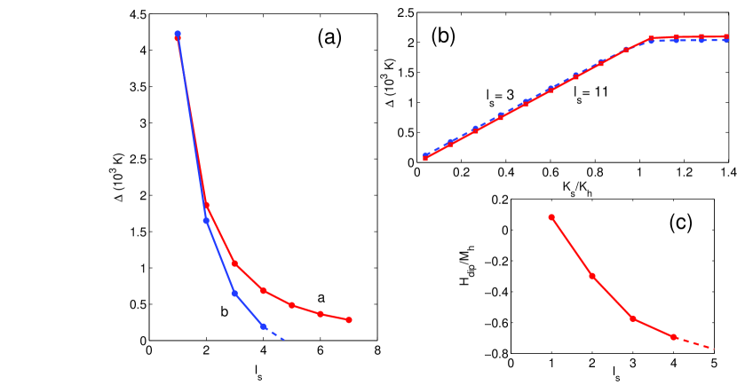
Figure 4: (a) Spin wave gap $\Delta$ (panel ) as a function of the the soft phase content $l_{s}$. The gap is calculated without (curve $a$) and with (curve $b$) the dipolar interaction term. (b) Spin wave gap $\Delta$ vs soft phase anisotropy parameter $K_{s}$ (normalized by $K_{h}$) for small ($l_{s}=3$) and large ($l_{s}=11$) amount of soft phase. (c) The effective demagnetizing field $H_{dip}$ (normalized by $M_{h}$) vs soft phase content $l_{s}$.

The effective demagnetizing field $H_{dip}$ is presented in Fig. 4(c). As expected, with increasing soft phase content $l_{s}$ the magnitude of the internal field increases due to increase of a magnetic charge forming at the hard-soft boundary. As a consequence, the whole manifold $E_{\bf k}$ displaces downward respective to $\varepsilon_{\bf k}$. When the dipolar field increases there is some critical amount of the soft phase $l_{s,c}$, beyond which a system with magnetic or structural nonhomogeneity would undergo the phase transition into another ground state with non-homogeneous distribution of the magnetization.

We finally present the dependence of $\Delta$ on the value of soft phase anisotropy parameter, $K_{s}$. The presented range of $K_{s}$ is much larger than that is in real soft magnets and was chosen to demonstrate the character of scaling of $\Delta$ with $K_{s}$. This dependence is illustrated in panel (b) of Fig. 4 for small, $l_{s}=3$, and large, $l_{s}=11$, amount of soft phase. The spin gap demonstrates a linear dependence on $K_{s}$, as long as $K_{s}<K_{h}$. It suggest that the main mechanism in formation of low-energy spin excitations in composite magnets is the interplay of the anisotropy and exchange interaction, as in the case of pure exchange spin waves, $\varepsilon_{\bf k}=2K+D{\bf k}^{2}$. The role of the dipolar interaction amounts to shifting of the spin-wave manifold as a whole and is crucial in the vicinity of $K_{s}\to 0$. This is the case for SmCo₅/FeCo composite, where $K_{s}\ll K_{h}$ and, as we have shown above, the spin excitations are mostly concentrated in the soft phase.

4 Conclusion

In this paper we studied the spin-wave spectra of two-phase ferromagnetic composites. Hard phase cubes inserted into a soft phase matrix form a 3D structure of exchange-coupled hard and soft phases. In such a geometry there are regions where the saturation magnetization $M_{S}({\bf r}){\hat{z}}$ is perpendicular to the hard-soft boundary, which is energetically unfavorable from the magnetostatic point of view. We have found the corresponding spin wave excitations and magnon wave functions by diagonalizing the Hamiltonian in the harmonic approximation.

We numerically found that low-lying excitations are mostly concentrated in the soft phase, which gives rise to considerable fluctuation of soft phase spins and a lack of the remanence enhancement with increasing of the soft phase amount. The spin wave frequencies strongly depend on the magnetic charges and magnetostatic interaction in the system. As it turns out the difference in the exchange coupling constants of hard and soft phase has little effect, if any, on the eigenmodes of the system. The energy of the lowest spin wave zone is mostly affected by the presence of the effective demagnetizing field in the composite and the value of anisotropy energy of the soft phase.

Finally, we have shown that with adding more soft phase the fully aligned spin state ${\bf M}({\bf r})=M_{S}({\bf r}){\hat{z}}$ becomes unstable relative to excitation of long wavelength spin waves with wave vector ${\bf k}$ parallel to the $z$ direction. The system undergoes a phase transition into another ground state characterized by misalignment of spins of hard and soft phases. We have found critical values of soft phase thickness $l_{s,c}$.

We thank G. Hadjipanayis and A. Gabay for helpful discussions. This work was supported in part by the U.S. Department of Energy (DOE) under the ARPA-E program (S.T.C.).

References

References

- [1] A.A. Serga, A.V. Chumak, and B. Hillebrands. J. Phys. D: Appl. Phys., 43:264002, 2010.
- [2] A.V. Chumak, T. Neumann, A.A. Serga, B. Hillebrands, and M. Kostylev. J. Phys. D: Appl. Phys., 42:205005, 2009.
- [3] B. Lenk, H. Ulrichs, F. Garbs, M. Munzenberg. Phys. Rep., 507:107, 2011.
- [4] P. Pirro, T. Brächer, A. V. Chumak, B. Lägel, C. Dubs, O. Surzhenko, P. Görnert, B. Leven, and B. Hillebrands. Appl. Phys. Lett., 104:012402, 2014.
- [5] M. B. Jungfleisch, W. Zhang, W. Jiang, H. Chang, J. Sklenar, S. M. Wu, J. E. Pearson, A. Bhattacharya, J. B. Ketterson, M. Wu and A. Hoffmann. J. Appl. Phys., 117:17D128, 2015.
- [6] G. Gubbiotti, S. Tacchi, G. Carlotti, P. Vavassori, N. Singh, S. Goolaup, A.O. Adeyeye, A. Stashkevich and M. Kostylev. Phys. Rev. B, 72:224413, 2005.
- [7] Z.K. Wang, V.L. Zhang, H.S. Lim, S.C. Ng, M.H. Kuok, S. Jain, and A.O. Adeyeye. Appl. Phys. Lett., 94:083112, 2009.
- [8] M. Bauer, C. Mathieu, S.O. Demokritov, B. Hillebrands, P.A. Kolodin, S. Sure, H. Dotsch, V. Grimalsky, Y. Rapoport, and A.N. Slavin. Phys. Rev. B, 56:R8483, 1997.
- [9] R. Zivieri, S. Tacchi, F. Montoncello, L. Giovannini, F. Nizzoli, M. Madami, G. Gubbiotti, G. Carlotti, S. Neusser, G. Duerr, and D. Grunder. Phys. Rev. B, 85:012403, 2012.
- [10] G. Gubbiotti, S. Tacchi, M. Madami, G. Carlotti, S. Jain, A.O. Adeyeye, and M. Kostylev. Appl. Phys. Lett., 100:162407, 2012.
- [11] S. Tacchi, F. Montoncello, M. Madami, G. Gubbiotti, G. Carlotti, L. Giovannini, R. Zivieri, F. Nizzoli, S. Jain, A.O. Adeyeye, and N. Singh. Phys. Rev. Lett., 107:127204, 2011.
- [12] R.H. Victora and X. Shen. IEEE Trans. Magn., 41:537, 2005.
- [13] E.F. Kneller and R. Hawig. IEEE Trans. Magn., 27:3588, 1991.
- [14] E.E. Fullerton, J.S. Jiang, M. Grimsditch, C.H. Sowers, and S.D. Bader. Phys. Rev. B, 58:12193, 1998.
- [15] R. Skomski and J.M.D. Coey. Phys. Rev. B, 48:15812, 1993.
- [16] A.M. Belemuk and S.T. Chui. J. Phys. D: Appl. Phys., 45:125001, 2012; A. M. Belemuk and S. T. Chui. J. Appl. Phys., 110:073918, 2011.
- [17] M. Krawczyk and H. Puszkarski. Phys. Rev. B, 77:054437, 2008.
- [18] M. Vohl, J. Barnas, and P. Grunberg. Phys. Rev. B, 39:12003, 1989.
- [19] R.P. Tiwari and D. Stroud. Phys. Rev. B, 81:220403, 2010.
- [20] A. Aharoni, Introduction to the Theory of Ferromagnetism. Oxford University Press, Oxford, 2000.
- [21] A. M. Belemuk and S. T. Chui. J. Appl. Phys., 113:043913, 2013.
- [22] R. Fischer, T. Leineweber, and H. Kronmuller. Phys. Rev. B, 57:10723, 1998.
- [23] R. Fischer and H. Kronmuller. Phys. Rev. B, 54:7284, 1996.
- [24] T. Schrefl, J. Fidler and H. Kronmuller. J. Magn. Magn. Mater., 138:15, 1994.
- [25] R. Fisher, T. Schrefl, H. Kronmuller and J. Fidler. J. Magn. Magn. Mater., 150:329, 1995.
- [26] A. M. Belemuk and S. T. Chui. J. Appl. Phys., 113:123906, 2013.
- [27] T. Holstein and H. Primakoff. Phys. Rev., 58:1098, 1940.
- [28] M.H. Cohen and F. Keffer. Phys. Rev., 99:1128, 1955.
- [29] N.M. Fujiki, K. De’Bell, and D.J.W. Gedart. Phys. Rev. B, 36:8512, 1987.
- [30] A. I. Akhiezer, V. G. Bar’yakhktar, S. V. Peletminskii, Spin Waves. North Holland, Amsterdam, 1968.
- [31] A.M. Clogston, H. Suhl, L.R. Walker and P.W. Anderson. J. Phys. Chem. Solids, 1:129, 1956.
- [32] A. L. Fetter. arXiv:cond-mat/9811366.
- [33] D.D. Stancil, A. Prabhakar, Spin waves. Springer, 2009.
- [34] C. Kittel, Quantum Theory of Solids. Wiley, 1987.
- [35] L.R. Walker. Phys. Rev., 105:390, 1957.
- [36] J.M.D. Coey, Magnetism and Magnetic Materials. Cambridge University Press, Cambridge, 2010.