Safe Pattern Pruning:
An Efficient Approach for Predictive Pattern Mining

Abstract

In this paper we study predictive pattern mining problems where the goal is to construct a predictive model based on a subset of predictive patterns in the database. Our main contribution is to introduce a novel method called safe pattern pruning (SPP) for a class of predictive pattern mining problems. The SPP method allows us to efficiently find a superset of all the predictive patterns in the database that are needed for the optimal predictive model. The advantage of the SPP method over existing boosting-type method is that the former can find the superset by a single search over the database, while the latter requires multiple searches. The SPP method is inspired by recent development of safe feature screening. In order to extend the idea of safe feature screening into predictive pattern mining, we derive a novel pruning rule called safe pattern pruning (SPP) rule that can be used for searching over the tree defined among patterns in the database. The SPP rule has a property that, if a node corresponding to a pattern in the database is pruned out by the SPP rule, then it is guaranteed that all the patterns corresponding to its descendant nodes are never needed for the optimal predictive model. We apply the SPP method to graph mining and item-set mining problems, and demonstrate its computational advantage.

Keywords

Predictive pattern mining, Graph mining, Item-set mining, Sparse learning, Safe screening, Convex optimization

1 Introduction

In this paper, we study predictive pattern mining. The goal of predictive pattern mining is discovering a set of patterns from databases that are needed for constructing a good predictive model. Predictive pattern mining problems can be interpreted as feature selection problems in supervised machine learning tasks such as classifications and regressions. The main difference between predictive pattern mining and ordinal feature selection is that, in the former, the number of possible patterns in databases are extremely large, meaning that we cannot naively search over all the patterns in databases. We thus need to develop algorithms that can exploit some structures among patterns such as trees or graphs for efficiently discovering good predictive patterns.

To be concrete, suppose that there are $D$ patterns in a database, which is assumed to be extremely large. For the $i$-th transaction in the database, let $z_{i1},\ldots,z_{iD}\in\{0,1\}$ represent the occurrence of each pattern. We consider linear predictive model in the form of

$$\sum_{j\in{\cal A}}w_{j}z_{ij}+b,$$ (1)

where ${\cal A}\subseteq\{1,\ldots,D\}$ is a set of patterns that would be selected by a mining algorithm, and $\{w_{j}\}_{j\in{\cal A}}$ and $b$ are the parameters of the linear predictive model. Here, the goal is to select a set of predictive patterns in ${\cal A}$ and find the model parameters $\{w_{j}\}_{j\in{\cal A}}$ and $b$ so that the predictive model in the form of (1) has good predictive ability.

Existing predictive pattern mining studies can be categorized into two approaches. The first approach is two-stage approach, where a mining algorithm is used for selecting the set of patterns ${\cal A}$ in the first stage, and the predictive model is fitted by only using the selected patterns in ${\cal A}$ in the second stage. Two-stage approach is computationally efficient because the mining algorithm is run only once in the first stage. However, two-stage approach is suboptimal as predictive model building procedure because it does not directly optimize the predictive model. The second approach is direct approach, where a mining algorithm is integrated in a feature selection method. An advantage of direct approach is that a set of patterns that are useful for predictive modeling is directly searched for. However, the computational cost of existing direct approach is usually much greater than two-stage approach because the mining algorithm is run multiple times. For example, in a stepwise feature selection method, the mining algorithm is run at each step in order for finding the pattern that best improves the current predictive model.

In this paper, we study a direct approach for predictive pattern mining based on sparse modeling. In the literature of machine-learning and statistics, sparse modeling has been intensively studied in the past two decades. An advantage of sparse modeling is that the problem is formulated as a convex optimization problem, and it allows us to investigate several properties of solutions from a wide variety of perspectives [1]. In addition, many efficient solvers that can be applicable to high-dimensional problems (although not as high as the number of patterns in databases as we consider in this paper) have been developed [2].

Predictive pattern mining algorithms based on sparse modeling have been also studied in the literature [3, 4, 5]. All these studies rely on a technique developed in the context of boosting [6]. Roughly speaking, in each step of the boosting-type method, a feature is selected based on a certain criteria, and an optimization problem defined over the set of features selected so far is solved. Therefore, when the boosting-type method is used for predictive pattern mining tasks, one has to search over the database as many times as the number of steps in the boosting-type method.

Our main contribution in this paper is to propose a novel method for sparse modeling-based predictive pattern mining. Denoting the set of patterns that would be used in the optimal predictive model as ${\cal A}^{*}$, the proposed method can find a set of patterns $\hat{{\cal A}}\supseteq{\cal A}^{*}$, i.e., $\hat{{\cal A}}$ contains all the predictive patterns that are needed for the optimal predictive model. It means that, if we solve the sparse modeling problem defined over the set of patterns $\hat{{\cal A}}$, then it is guaranteed that the resulting predictive model is optimal. The main advantage of the proposed method over the above boosting-type method is that a mining algorithm is run only once for finding the set of patterns $\hat{{\cal A}}$.

The proposed method is inspired by recent safe feature screening studies [7, 8, 9, 10, 11, 12, 13, 14, 15]. In ordinary feature selection problems, safe feature screening allows us to identify a set of features that would never be used in the optimal model before actually solving the optimization problem It means that these features can be safely removed from the training set. Unfortunately, however, it cannot be applied to predictive pattern mining problems because it is computationally intractable to apply safe feature screening to each of extremely large number of patterns in a database for checking whether the pattern can be safely removed out or not.

In this paper, we develop a novel method called safe pattern pruning (SPP). Considering a tree structure defined among patterns in the database, the SPP method allows us to prune the tree in such a way that, if a node corresponding to a pattern in the database is pruned out, then it is guaranteed that all the patterns corresponding to its descendant nodes would never be needed for the optimal predictive model. The SPP method can be effectively used in predictive pattern mining problems because we can identify an extremely large set of patterns that are irrelevant to the optimal predictive model by exploiting the tree structure among patterns in the database, A superset $\hat{{\cal A}}\supseteq{\cal A}^{*}$ can be obtained by collecting the set of patterns corresponding to the nodes that are not pruned out by the SPP method.

1.1 Notation and outline

We use the following notations in the rest of the paper. For any natural number $n$, we define $[n]:=\{1,\ldots,n\}$. For an $n$-dimensional vector $\bm{v}$ and a set ${\cal I}\subseteq[n]$, $\bm{v}_{{\cal I}}$ represents a sub-vector of $\bm{v}$ whose elements are index by ${\cal I}$. The indicator function is written as $I(\cdot)$, i.e., $I(z)=1$ if $z$ is true, and $I(z)=0$ otherwise. Boldface $\bm{0}$ and $\bm{1}$ indicate a vector of all zeros and ones, respectively.

Here is the outline of the paper. §2 presents problem setup and existing methods. §3 describes our main contribution where we introduce safe pattern pruning (SPP) method. §4 covers numerical experiments for demonstrating the advantage of the SPP method. §5 concludes the paper.

2 Preliminaries

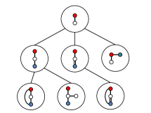
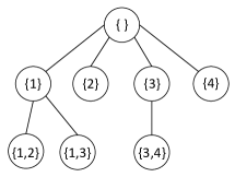
(a) Graph mining					(b) Item-set mining

Figure 1: Two examples of tree structures defined among patterns in databases.

We first formulate our problem setting.

2.1 Problem setup

In this paper we consider predictive pattern mining problems. Let us consider a database with $n$ records, and denote the dataset as $\{(G_{i},y_{i})\}_{i\in[n]}$, where $G_{i}$ is a labeled undirected graph in the case of graph mining, while it is a set of items in the case of item-set mining. The response variable $y_{i}$ is defined on $\mathbb{R}$ and on $\{\pm 1\}$ for regression and classification problems, respectively. Let ${\cal T}$ be the set of all patterns in the database, and denote its size as $D:=|{\cal T}|$. For example, ${\cal T}$ is the set of all possible subgraphs in the case of graph mining, while ${\cal T}$ is the set of all possible item-sets in the case of item-set mining. Alternatively, $G_{i}$ is represented as a $D$-dimensional binary vector $\bm{x}_{i}\in\{0,1\}^{D}$ whose $t$-th element is defined as

$$x_{it}:=I(t\subseteq G_{i}),~{}\forall t\in{\cal T}.$$

The number of patterns $D$ is extremely large in all practical pattern mining problems. It implies that any algorithms that naively search over all $D$ patterns are computationally infeasible.

In order to study both regression and classification problems in a unified framework, we consider the following class of convex optimization problems:

$$\min_{\bm{w},b}P_{\lambda}(\bm{w},b):=\sum_{i\in[n]}f(\bm{\alpha}_{i}^{\top}\bm{w}+\beta_{i}b+\gamma_{i})+\lambda\|\bm{w}\|_{1},$$ (2)

where $f:\mathbb{R}\to\mathbb{R}$ is a gradient Lipschitz continuous loss function and $\lambda>0$ is a tuning parameter. We refer the problem (2) as primal problem and write the optimal solution as $\bm{w}^{*}$. When $f(z):=\frac{1}{2}z^{2}$ and $\bm{\alpha}_{i}:=\bm{x}_{i}$, $\beta_{i}:=1$, $\gamma_{i}:=-y_{i}$ $\forall i\in[n]$, the general problem (2) is reduced to the following $L_{1}$-penalized regression problem defined over $D+1$ variables:

$$\min_{\bm{w}\in\mathbb{R}^{D},b\in\mathbb{R}}~{}\frac{1}{2}\sum_{i\in[n]}(\bm{x}_{i}^{\top}\bm{w}+b-y_{i})^{2}+\lambda\|\bm{w}\|_{1}.$$ (3)

On the other hand, when $f(z):=\frac{1}{2}\max\{0,1-z\}^{2}$ and $\bm{\alpha}_{i}:=y_{i}\bm{x}_{i}$, $\beta_{i}:=y_{i}$, $\gamma_{i}:=0$ $\forall i\in[n]$, the general problem (2) is reduced to the following $L_{1}$-penalized classification problem defined over $D+1$ variables:

$$\min_{\bm{w}\in\mathbb{R}^{D},b\in\mathbb{R}}~{}\frac{1}{2}\sum_{i\in[n]}\max\{0,1-y_{i}(\bm{x}_{i}^{\top}\bm{w}+b)\}^{2}+\lambda\|\bm{w}\|_{1}.$$ (4)

Remembering that $D$ is extremely large, we cannot solve these $L_{1}$-penalized regression and classification problems in a standard way.

The dual problem of (2) is defined as

$$\begin{aligned} \max_{\bm{\theta}\in\mathbb{R}^{n}}~{}D_{\lambda}(\bm{\theta}):=-\frac{\lambda^{2}}{2}\|\bm{\theta}\|_{2}^{2}+\lambda\bm{\delta}^{\top}\bm{\theta}\\ {\rm s.t.}~{}\left|\sum_{i\in[n]}\alpha_{it}\theta_{i}\right|\leq 1,\forall t\in{\cal T},\\ \bm{\beta}^{\top}\bm{\theta}=0,~{}\theta_{i}\geq\varepsilon,~{}\forall i\in[n],\end{aligned}$$ (5)

where $\bm{\delta}=\bm{y}$, $\varepsilon=-\infty$ for regression problem in (3), and $\bm{\delta}=\bm{1}$, $\varepsilon=0$ for classification problem in (4). The dual optimal solution is denoted as $\bm{\theta}^{*}$.

The key idea for handling an extremely large number of patterns in the database is to exploit the tree structure defined among the patterns. Figure 1 shows tree structures for graph mining (left) and item-set mining (right). As shown in Figure 1, each node of the tree corresponds to each pattern in the database. Those trees are constructed in such a way that, for any pair of a node $t$ and one of its descendant node $t^{\prime}$, they satisfy the relation $t\subseteq t^{\prime}$, i.e., the pattern $t^{\prime}$ is a superset of the pattern $t$. It suggests that, for such a pair of $t$ and $t^{\prime}$,

$$x_{it^{\prime}}=1~{}\Rightarrow~{}x_{it}=1~{}~{}~{}\forall i,$$

and, conversely

$$x_{it}=0~{}\Rightarrow~{}x_{it^{\prime}}=0~{}~{}~{}\forall i.$$

2.2 Existing method

To the best of our knowledge, except for the boosting-type method described in §1 and its extensions or modifications [3, 4, 5], there is no other existing method that can be used for solving the convex optimization problem (2) for predictive pattern mining problems defined over an extremely large number of patterns $D$. The boosting-type method solves the dual problem (5). The difficulty in the dual problem is that there are extremely large number of constraints in the form of $|\sum_{i\in[n]}\alpha_{it}\theta_{i}|\leq 1,\forall t\in{\cal T}$. Starting from the optimization problem (5) without these constraints, in each step of the boosting-type method, the most violating constraint is added to the problem, and an optimization problem only with the constraints added so far is solved. In optimization literature, this approach is generally known as the cutting-plane method, for which its effectiveness has been also shown in some machine learning problems (e.g., [16]). The key computational trick used by [3, 4, 5] is that, for finding the most violating constraint in each step, it is possible to efficiently search over the database by using a certain pruning strategy in the tree as depicted in Figure 1. This method is terminated when there is no violating constraints in the database.

In each single step of the boosting-type method, one first has to search over the database by a mining algorithm, and then run a convex optimization solver for the problem with the newly added constraint. Boosting-type method is computationally expensive because these steps must be repeated until all the constraints corresponding to all the predictive patterns in ${\cal A}^{*}$ are added. In the next section, we propose a novel method called safe pattern pruning, by which the optimal model is obtained by a single search over the database and a single run of convex optimization solver.

3 Safe pattern pruning

In this section, we present our main contribution.

3.1 Basic idea

It is well known that $L_{1}$ penalization in (2) makes the solution $\bm{w}^{*}$ sparse, i.e., some of its element would be zero. The set of patterns which has non-zero coefficients are called active and denoted as ${\cal A}^{*}\subseteq{\cal T}$, while the rest of the patterns are called non-active. A nice property of sparse learning is that the optimal solution does not depend on any non-active patterns. It means that, after some non-active patterns are removed out from the dataset, the same optimal solution can be obtained. The following lemma formally states this well-known but important fact.

Lemma 1.

Let $\hat{{\cal A}}$ be a set such that ${\cal A}^{*}\subseteq\hat{{\cal A}}\subseteq{\cal T}$, and $P_{\lambda}^{\hat{{\cal A}}}(\bm{w}_{\hat{{\cal A}}},b)$ be the objective function of (2) in which $\bm{w}_{{\cal T}\setminus\hat{{\cal A}}}=\bm{0}$ is substituted:

$$P_{\lambda}^{\hat{{\cal A}}}(\bm{w}_{\hat{{\cal A}}},b):=\sum_{i\in[n]}f(\bm{\alpha}_{\hat{{\cal A}},i}^{\top}\bm{w}_{\hat{{\cal A}}}+\beta_{i}b+\gamma_{i})+\lambda\|\bm{w}_{\hat{{\cal A}}}\|_{1}.$$ (6)

Then, the optimal solution of the original problem (2) is given by

$$(\bm{w}^{*}_{\hat{{\cal A}}},b) =\arg\min_{\bm{w}_{\hat{{\cal A}}}\in\mathbb{R}^{|\hat{{\cal A}}|},b\in\mathbb{R}}~{}P_{\lambda}^{\hat{{\cal A}}}(\bm{w}_{\hat{{\cal A}}},b),$$

$$\bm{w}^{*}_{{\cal T}\setminus\hat{{\cal A}}} =\bm{0}.$$

Lemma 1 indicates that, if we have a set of patterns $\hat{{\cal A}}\supseteq{\cal A}^{*}$, we have only to solve a smaller optimization problem defined only with the set of patterns in $\hat{{\cal A}}$. It means that, if such an $\hat{{\cal A}}$ is available, we do not have to work with extremely large number of patterns in the database.

In the rest of this section, we propose a novel method for finding such a set of patterns $\hat{{\cal A}}\supseteq{\cal A}^{*}$ by searching over the database only once. Specifically, we derive a novel pruning condition which has a property that, if the condition is satisfied at a certain node, then all the patterns corresponding to its descendant nodes and the node itself are guaranteed to be non-active. After traversing the tree, we simply define $\hat{{\cal A}}$ be the set of nodes which are not pruned out. Then, it is guaranteed that $\hat{{\cal A}}$ satisfies the condition in Lemma 1. The proposed method is inspired by recent studies on safe feature screening. We thus call our new method as safe pattern pruning (SPP).

3.2 Main theorem for safe pattern pruning

The following theorem provides a specific pruning condition that can be used together with any search strategies on a tree. Let ${\cal T}_{\rm sub}(t)\subseteq{\cal T}$ be a set of nodes in a subtree of ${\cal T}$ having $t$ as a root node and containing all descendant nodes of $t$. We derive a condition for safely screening the entire ${\cal T}_{\rm sub}(t)$ out, which is computable at the node $t$ without traversing the descendant nodes. This means that, our rule, called safe pattern pruning rule, tells us whether a pattern $t^{\prime}$ $\in{\cal T}_{\rm sub}(t)$ has a chance to be active or not based on the information available at the root node of the subtree $t$. An important consequence of the condition below is that if the condition holds, i.e., any $t^{\prime}\in{\cal T}_{\rm sub}(t)$ cannot be active, then we can stop searching over the subtree (pruning the subtree).

Theorem 2 (Safe pattern pruning (SPP) rule).

Given an arbitrary primal feasible solution $(\tilde{\bm{w}},\tilde{b})$ and an arbitrary dual feasible solution $\tilde{\bm{\theta}}$, for any node $t^{\prime}\in{\cal T}_{\rm sub}(t)$, the following safe pattern pruning criterion (SPPC) provides a rule

$${\rm SPPC}(t):=u_{t}+r_{\lambda}\sqrt{v_{t}}<1~{}\Rightarrow~{}w^{*}_{t^{\prime}}=0,$$

where

$$u_{t}:=\max\left\{\sum_{i:\beta_{i}\tilde{\theta}_{i}>0}\alpha_{it}\tilde{\theta}_{i},~{}-\sum_{i:\beta_{i}\tilde{\theta}_{i}<0}\alpha_{it}\tilde{\theta}_{i}\right\},~{}v_{t}:=\sum_{i\in[n]}\alpha_{it}^{2},$$

for $t\in[D]$, and

$$r_{\lambda}:=\frac{\sqrt{2(P_{\lambda}(\tilde{\bm{w}},\tilde{b})-D_{\lambda}(\tilde{\bm{\theta}}))}}{\lambda}.$$

The proof of Theorem 2 is presented in §3.3.

${\rm SPPC}(t)$ depends on three scalar quantities $u_{t}$, $v_{t}$ and $r_{\lambda}$. The first two quantities $u_{t}$ and $v_{t}$ are obtained by using information on the pattern $t$, while the third quantity $r_{\lambda}$ does not depend on $t$. Noting that all these three quantities are non-negative, the SPP rule would be more powerful (have more chance to prune the subtree) if these three quantities are smaller. The following corollary is the consequence of the simple fact that the first two quantities $u_{t}$ and $v_{t}$ at a descendant node are smaller than those at its ancestor nodes.

Corollary 3.

For any node $t^{\prime}\in{\cal T}_{\rm sub}(t)$,

$${\rm SPPC}(t)\geq{\rm SPPC}(t^{\prime})$$

The proof of Corollary 3 is presented in Appendix. This corollary suggests that the SPP rule would be more powerful at deeper nodes.

The third quantity $r_{\lambda}$ represents the goodness of the pair of primal and dual feasible solutions measured by the duality gap, the difference between the primal and dual objective values. It means that, if sufficiently good pair of primal and dual feasible solutions are available, the SPP rule would be powerful. We will discuss how to obtain good feasible solutions in §3.4.

3.3 Proof of Theorem 2

In order to prove Theorem 2, we first clarify the condition for any pattern $t\in{\cal T}$ to be non-active by the following lemma.

Lemma 4.

For a pattern $t\in{\cal T}$,

$$\left|\sum_{i\in[n]}\alpha_{it}\theta^{*}_{i}\right|<1~{}\Rightarrow~{}w^{*}_{t}=0.$$

Proof of Lemma 4 is presented in Appendix. Lemma 4 indicates that, if an upper bound of $|\sum_{i\in[n]}\alpha_{it}\theta_{i}^{*}|$ is smaller than 1, then we can guarantee that $w^{*}_{t}=0$. In what follows, we actually show that SPPC($t$) is an upper bound of $|\sum_{i\in[n]}\alpha_{it^{\prime}}\theta_{i}^{*}|$ for $\forall t^{\prime}\in{\cal T}_{\rm sub}(t)$.

In order to derive an upper bound of $|\sum_{i\in[n]}\alpha_{it}\theta_{i}^{*}|$, we use a technique developed in a recent safe feature screening study [15]. The following lemma states that, based on a pair of a primal feasible solution $(\tilde{\bm{w}},\tilde{b})$ and a dual feasible solution $\tilde{\bm{\theta}}$, we can find a ball in the dual solution space $\mathbb{R}^{n}$ in which the dual optimal solution $\bm{\theta}^{*}$ exists.

Lemma 5 (Theorem 3 in [15]).

Let $(\tilde{\bm{w}},\tilde{b})$ be an arbitrary primal feasible solution, and $\tilde{\bm{\theta}}$ be an arbitrary dual feasible solution. Then, the dual optimal solution $\bm{\theta}^{*}$ is within a ball in the dual solution space $\mathbb{R}^{n}$ with the center $\tilde{\bm{\theta}}$ and the radius $r_{\lambda}:=\sqrt{2(P_{\lambda}(\tilde{\bm{w}},\tilde{b})-D_{\lambda}(\tilde{\bm{\theta}}))}/\lambda$.

See Theorem 3 and its proof in [15]. This lemma tells that, given a pair of primal feasible and dual feasible solutions, we can bound the dual optimal solution within a ball.

Lemma 5 can be used for deriving an upper bound of $|\sum_{i\in[n]}\alpha_{it}\theta_{i}^{*}|$. Since we know that the dual optimal solution $\bm{\theta}^{*}$ is within the ball in Lemma 5, an upper bound of any $t\in{\cal T}$ can be obtained by solving the following convex optimization problem:

$$\begin{aligned} {\rm UB}(t):=\arg\max_{\bm{\theta}\in\mathbb{R}^{n}}&~{}\left|\sum_{i\in[n]}\alpha_{it}\theta_{i}\right|\\ {\rm s.t.}&~{}\left\|\bm{\theta}-\tilde{\bm{\theta}}\right\|_{2}\leq\sqrt{2(P_{\lambda}(\tilde{\bm{w}},\tilde{b})-D_{\lambda}(\tilde{\bm{\theta}}))}/\lambda,\\ &\bm{\beta}^{\top}\bm{\theta}=0.\end{aligned}$$ (7)

Fortunately, the convex optimization problem (7) can be explicitly solved as the following lemma states.

Lemma 6.

The solution of the convex optimization problem (7) is given as

$${\rm UB}(t)=\left|\sum_{i\in[n]}\alpha_{it}\tilde{\theta}_{i}\right|+r_{\lambda}\sqrt{\sum_{i\in[n]}\alpha_{it}^{2}-\frac{(\sum_{i\in[n]}\alpha_{it}\beta_{i})^{2}}{\|\bm{\beta}\|_{2}^{2}}}.$$

Proof of Lemma 6 is presented in Appendix.

Although ${\rm UB}(t)$ provides a condition to screen any $t\in{\cal T}$, calculating ${\rm UB}(t)$ for all $t\in{\cal T}$ is computationally prohibiting in our extremely high dimensional problem setting. In the next lemma, we will show that ${\rm SPPC}(t)\geq{\rm UB}(t^{\prime})$ for $\forall t^{\prime}\in{\cal T}_{\rm sub}(t)$, i.e., ${\rm SPPC}(t)$ in Theorem 2 is an upper bound of ${\rm UB}(t^{\prime})$, which enables us to efficiently prune subtrees during the tree traverse process.

Lemma 7.

For any $t^{\prime}\in{\cal T}_{\rm sub}(t)$,

Finally, by combining Lemmas 4, 5, 6 and 7, we can prove Theorem 2.

Proof of Theorem 2.

Proof.

From Lemmas 5, 6 and 7,

$$\left|\sum_{i\in[n]}\alpha_{it^{\prime}}\theta_{i}^{*}\right|\leq{\rm UB}(t^{\prime})\leq{\rm SPPC}(t),~{}~{}~{}\forall t^{\prime}\in{\cal T}_{\rm sub}(t).$$ (8)

From Lemma 4 and (8),

$${\rm SPPC}(t)<1~{}\Rightarrow~{}w^{*}_{t^{\prime}}=0,~{}~{}~{}\forall t^{\prime}\in{\cal T}_{\rm sub}(t).$$

∎

Algorithm 1 Regularization path computation algorithm

0:  $\{(G_{i},y_{i})\}_{i\in[n]}$, $\{\lambda_{k}\}_{k\in[K]}$

1:  $\lambda_{0}\leftarrow\max_{t\in{\cal T}}\left|\sum_{i\in[n]}x_{it}(y_{i}-\bar{y})\right|$ and $(\bm{w}_{0},b_{0})\leftarrow(\bm{0},\bar{y})$

2:  for $k=1,\ldots,K$ do

3:     Find $\hat{{\cal A}}(\lambda_{k})\supseteq{\cal A}^{*}(\lambda_{k})$ by searching over the tree with the SPP rules based on $(\bm{w}^{*}(\lambda_{k-1}),b^{*}(\lambda_{k-1}))$ and $\bm{\theta}^{*}(\lambda_{k-1})$ as the primal and dual feasible solutions, respectively.

4:     Solve a small optimization problems in (6) with $\hat{{\cal A}}=\hat{{\cal A}}(\lambda_{k})$, and obtain the primal solution $(\bm{w}^{*}(\lambda_{k}),b^{*}(\lambda_{k}))$ and the dual solution $\bm{\theta}^{*}(\lambda_{k})$.

5:  end for

5:  $\{(\bm{w}^{*}(\lambda_{k}),b^{*}(\lambda_{k}))\}_{k\in[K]}$ and $\{(\bm{\theta}^{*}(\lambda_{k})\}_{k\in[K]}$

3.4 Practical considerations

Safe pattern pruning rule in Theorem 2 depends on a pair of a primal feasible solution $(\tilde{\bm{w}},\tilde{b})$ and a dual feasible solution $\tilde{\bm{\theta}}$. Although the rule can be constructed from any solutions as long as they are feasible, the power of the rule depends on the goodness of these solutions. Specifically, the criterion ${\rm SPPC}(t)$ depends on the duality gap $P_{\lambda}(\tilde{\bm{w}},\tilde{b})-D_{\lambda}(\tilde{\bm{\theta}})$ which would vanish when these primal and dual solutions are optimal. Roughly speaking, it suggests that, if these solutions are somewhat close to the optimal ones, we could expect that the SPP rule is powerful.

3.4.1 Computing regularization path

In practical predictive pattern mining tasks, we need to find a good penalty parameter $\lambda$ based on a model selection technique such as cross-validation. In model selection, a sequence of solutions with various different penalty parameters must be trained. Such a sequence of the solutions is sometimes referred to as a regularization path [17]. Regularization path of the problem (2) is usually computed from larger $\lambda$ to smaller $\lambda$ because more sparse solutions would be obtained for larger $\lambda$. Let us write the sequence of $\lambda$s as $\lambda_{0}>\lambda_{1}>\ldots>\lambda_{K}$. When computing such a sequence of solutions, it is reasonable to use warm-start approach where the previous optimal solution at $\lambda_{k-1}$ is used as the initial starting point of the next optimization problem at $\lambda_{k}$. In such a situation, we can also make use of the previous solution at $\lambda_{k-1}$ as the feasible solution for the safe pattern pruning rule at $\lambda_{k}$.

In sparse modeling literature, it is custom to start from the largest possible $\lambda$ at which the primal solution is given as $\bm{w}^{*}=\bm{0}$ and $b^{*}=\bar{y}$, where $\bar{y}$ is the sample mean of $\{y_{i}\}_{i\in[n]}$. The largest $\lambda$ is given as

$$\lambda_{\rm max}:=\max_{t\in{\cal T}}\left|\sum_{i\in[n]}x_{it}(y_{i}-\bar{y})\right|.$$

In order to solve this maximization problem over the database, for a node $t$ and $t^{\prime}\in{\cal T}_{\rm sub}(t)$, we can use the following upper bound

$$\begin{aligned} &\left|\sum_{i\in[n]}x_{it^{\prime}}(y_{i}-\bar{y})\right|\\ &~{}~{}~{}~{}~{}\leq\max\left\{\sum_{i\mid y_{i}-\bar{y}>0}x_{it}(y_{i}-\bar{y}),-\sum_{i\mid y_{i}-\bar{y}<0}x_{it}(y_{i}-\bar{y})\right\},\end{aligned}$$

and this upper bound can be exploited for pruning the search over the tree.

Algorithm 1 shows the entire procedure for computing the regularization path by using the SPP rule.

4 Experiments

In this section, we demonstrate the effectiveness of the proposed safe pattern pruning (SPP) method through numerical experiments. We compare SPP with the boosting-based method (boosting) discussed in §2.2.

4.1 Experimental setup

We considered regularization path computation scenario described in §3.4.1. Specifically, we computed a sequence of optimal solutions of (2) for a sequence of 100 penalty parameters $\lambda$ evenly allocated between $\lambda_{0}=\lambda_{\rm max}$ and $0.01\lambda_{0}$ in logarithmic scale. For solving the convex optimization problems, we used coordinate gradient descent method [18]. The optimization solver was terminated when the duality gap felled below $10^{-6}$. In both of SPP and boosting, we used warm-start approach. In addition, the solution at the previous $\lambda$ was also used as the feasible solution for constructing the SPP rule at the next $\lambda$. We used gSpan algorithm [19] for mining subgraphs. We wrote all the codes (except gSpan part in graph mining experiment) in C++. All the computations were conducted by using a single core of an Intel Xeon CPU E5-2643 v2 (3.50GHz) with 64GB MEM.

4.2 Graph classification/regression

We applied SPP and boosting to graph classification and regression problems. For classification, we used CPDB and mutagenicity datasets, containing $n=648$ and $n=4377$ chemical compounds respectively, for which the goal is to predict whether each compound has mutagenicity or not. For regression, we used Bergstrom and Karthikeyan datasets where the goal is to predict the melting point of each of the $n=185$ and $n=4173$ chemical compounds. All datasets are downloadable from http://cheminformatics.org/datasets/.
We considered the cases with maxpat $\in\{5,6,7,8,9,10\}$, where maxpat indicates the maximum number of edges of subgraphs we wanted to find.

Figure 2 shows the computation time of the two methods. In all the cases, SPP is faster than boosting, and the difference gets larger as maxpat increases. Figure 2 also shows the computation time taken in traversing the trees (traverse) and that taken in solving the optimization problems (solve). The results indicate that traverse time of SPP are only slightly better than that of boosting. It is because the most time-consuming component of gSpan is the minimality check of the DFS (depth-first search) code, and the traverse time mainly depends on how many different nodes are generated in the entire regularization path computation process. In terms of solve time, there are large difference between SPP and boosting. In SPP, we have only to solve a single convex optimization problem for each $\lambda$. In boosting, on the other hand, convex optimization problems must be repeatedly solved every time a new pattern is added to the working set. Figure 4 shows the total number of traversed nodes in the entire regularization path computation process. Total number of traversed nodes in SPP is much smaller than those of boosting, which is because one must repeat searching over trees many times in boosting.

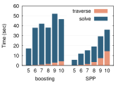
(a) CPDB

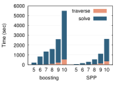
(b) mutagenicity

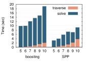
(c) Bergstrom

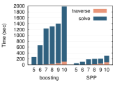
(d) Karthikeyan

Figure 2: Computation time comparison for graph classification and regression. Each bar contains computational time taken in the tree traverse (traverse) and the optimization procedure (solve) respectively.

4.3 Item-set classification/regression

We applied SPP and boosting to item-set classification and regression problems. For classification, we used splice dataset ($n=1000$ and the number of items $d=120$) and a9a dataset ($n=32561$ and $d=123$). For regression, we used dna dataset ($n=2000$ and $d=180$) and protein dataset ($n=6621$ and $d=714$). All datasets were obtained from LIBSVM Dataset site [20]. We considered the cases with maxpat $\in\{3,4,5,6\}$, where maxpat here indicates the maximum size of item-sets we wanted to find.

Figure 3 compares the computation time of the two methods. In all the cases, SPP is faster than boosting. Here again, Figure 3 also shows the computation time taken in traversing the trees (traverse) and that taken in solving the optimization problems (solve). In contrast to the graph mining results, traverse time of SPP are much smaller than that of boosting because it simply depends on how many nodes are traversed in total. Figure 5 shows the total number of traversed nodes in the entire regularization path computation process. Especially when $\lambda$ is small where the number of active patterns are large, boosting needed to traverse large number of nodes, which is because the number of steps of boosting is large when there are large number of active patterns.

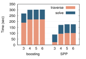
(a) splice

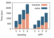
(b) a9a

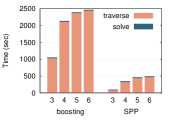
(c) dna

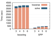
(d) protein

Figure 3: Computation time comparison for item-set classification and regression. Each bar contains computational time taken in the tree traverse (traverse) and the optimization procedure (solve) respectively.

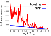
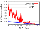
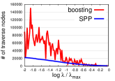
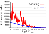
(a-1) maxpat 6	(a-2) maxpat 7	(a-3) maxpat 8	(a-4) maxpat 10

(a) CPDB

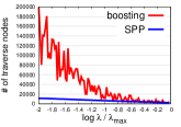
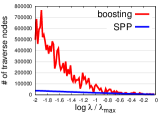
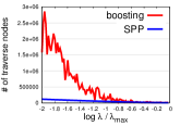
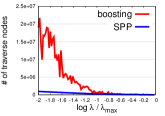
(b-1) maxpat 6	(b-2) maxpat 7	(b-3) maxpat 8	(b-4) maxpat 10

(b) mutagenicity

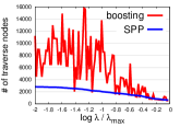
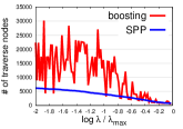
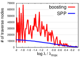
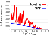
(c-1) maxpat 6	(c-2) maxpat 7	(c-3) maxpat 8	(c-4) maxpat 10

(c) Bergstrom

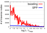
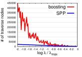
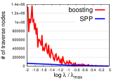
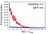
(d-1) maxpat 6	(d-2) maxpat 7	(d-3) maxpat 8	(d-4) maxpat 10

(d) Karthikeyan

Figure 4: # of traverse nodes for graph classification and regression.

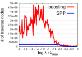
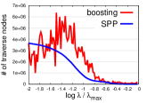
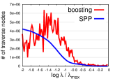
(a-1) maxpat 3	(a-2) maxpat 4	(a-3) maxpat 5	(a-4) maxpat 6

(a) splice

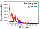
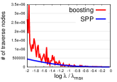
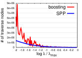
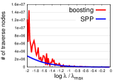
(b-1) maxpat 3	(b-2) maxpat 4	(b-2) maxpat 5	(b-3) maxpat 6

(b) a9a

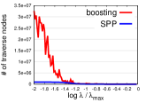
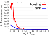
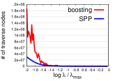
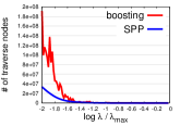
(c-1) maxpat 3	(c-2) maxpat 4	(c-3) maxpat 5	(c-4) maxpat 6

(c) dna

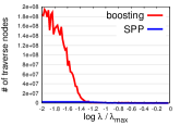
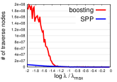
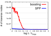
(d-1) maxpat 3	(d-2) maxpat 4	(d-3) maxpat 5	(d-4) maxpat 6

(d) protein

Figure 5: # of traverse nodes for item-set classification and regression.

5 Conclusions

In this paper, we introduced a novel method called safe pattern pruning (SPP) method for a class of predictive pattern mining problems. The advantage of the SPP method is that it allows us to efficiently find a superset of all the predictive patterns that are used in the optimal predictive model by a single search over the database. We demonstrated the computational advantage of the SPP method by applying it to graph classification/regression and item-set classification/regression problems. As a future work, we will study how to integrate the SPP method with a technique for providing the statistical significances of the discovered patterns [21, 22].

Appendix A Proofs

Proof of Corollary 3

Proof.

For any pair of a node $t$ and $t^{\prime}\in{\cal T}_{\rm sub}(t)$,

$$\sum_{i:\beta_{i}\tilde{\theta}_{i}>0}\alpha_{it}\tilde{\theta}_{i}\geq\sum_{i:\beta_{i}\tilde{\theta}_{i}>0}\alpha_{it^{\prime}}\tilde{\theta}_{i},$$ (9)

$$\sum_{i:\beta_{i}\tilde{\theta}_{i}<0}\alpha_{it}\tilde{\theta}_{i}\leq\sum_{i:\beta_{i}\tilde{\theta}_{i}<0}\alpha_{it^{\prime}}\tilde{\theta}_{i}.$$ (10)

First consider the case where $u_{t}=\sum_{i:\beta_{i}\tilde{\theta}_{i}>0}\alpha_{it}\tilde{\theta}_{i}$. When $u_{t^{\prime}}=\sum_{i:\beta_{i}\tilde{\theta}_{i}>0}\alpha_{it^{\prime}}\tilde{\theta}_{i}$, from (9), $u_{t}\geq u_{t^{\prime}}$. When $u_{t^{\prime}}=-\sum_{i:\beta_{i}\tilde{\theta}_{i}<0}\alpha_{it^{\prime}}\tilde{\theta}_{i}$, from (10),

$$u_{t}\geq-\sum_{i:\beta_{i}\tilde{\theta}_{i}<0}\alpha_{it}\tilde{\theta}_{i}\geq u_{t^{\prime}}.$$

Next, consider the case where $u_{t}=-\sum_{i:\beta_{i}\tilde{\theta}_{i}<0}\alpha_{it}\tilde{\theta}_{i}$. When $u_{t^{\prime}}=\sum_{i:\beta_{i}\tilde{\theta}_{i}>0}\alpha_{it^{\prime}}\tilde{\theta}_{i}$, from (9),

$$u_{t}\geq\sum_{i:\beta_{i}\tilde{\theta}_{i}<0}\alpha_{it}\tilde{\theta}_{i}\geq u_{t^{\prime}}.$$

When $u_{t^{\prime}}=-\sum_{i:\beta_{i}\tilde{\theta}_{i}<0}\alpha_{it^{\prime}}\tilde{\theta}_{i}$, from (10), $u_{t}\geq u_{t^{\prime}}$. Furthermore, it is clear that $v_{t}\geq v_{t^{\prime}}$. Since $r_{\lambda}>0$, ${\rm SPPC}(t)\geq{\rm SPPC}(t^{\prime})$. ∎

Proof of Lemma 4

Proof.

Based on the convex optimization theory (see, e.g., [23]), the KKT optimality condition of the primal problem (2) and the dual problem (5) is written as

$$\sum_{i=1}^{n}\alpha_{it}\theta_{i}^{*}\in\begin{cases}{\rm sign}(w_{t}^{*})&{\rm if~{}}w_{t}^{*}\neq 0,\\ [-1,+1]&{\rm if~{}}w_{t}^{*}=0,\end{cases}~{}~{}\forall t\in{\cal T}.$$

It suggests that

$$\left|\sum_{i=1}^{n}\alpha_{it}\theta_{i}^{*}\right|<1~{}\Rightarrow~{}w_{t}^{*}=0,~{}\forall t\in{\cal T}.$$

∎

Proof of Lemma 6

Proof.

Let $\bm{\alpha}_{:,t}:=[\alpha_{1t},\ldots,\alpha_{nt}]^{\top}$. First, note that the objective part of the optimization problem (7) is rewritten as

$$\max_{\bm{\theta}}~{}\left|\bm{\alpha}_{:,t}^{\top}\bm{\theta}\right|$$

$$~{}\Leftrightarrow~{} \max_{\bm{\theta}}\max\left\{\bm{\alpha}_{:,t}^{\top}\bm{\theta},-\bm{\alpha}_{:,t}^{\top}\bm{\theta}\right\}$$

$$~{}\Leftrightarrow~{} \max\left\{-\min_{\bm{\theta}}(-\bm{\alpha}_{:,t})^{\top}\bm{\theta},-\min_{\bm{\theta}}\bm{\alpha}_{:,t}^{\top}\bm{\theta}\right\}$$ (11)

Thus, we consider the following convex optimization problem:

$$\min_{\bm{\theta}}~{}\bm{\alpha}_{:,t}^{\top}\bm{\theta}~{}{\rm s.t.}~{}\|\bm{\theta}-\tilde{\bm{\theta}}\|_{2}^{2}\leq r_{\lambda}^{2},\bm{\beta}^{\top}\bm{\theta}=0.$$ (12)

Let us define the Lagrange function

$$L(\bm{\theta},\xi,\eta)=\bm{\alpha}_{:,t}^{\top}\bm{\theta}+\xi(\|\bm{\theta}-\tilde{\bm{\theta}}\|^{2}_{2}-r_{\lambda}^{2})+\eta\bm{\beta}^{\top}\bm{\theta},$$

and then the optimization problem (12) is written as

$$\min_{\bm{\theta}}\max_{\xi\geq 0,\eta}L(\bm{\theta},\xi,\eta).$$ (13)

The KKT optimality conditions are summarized as

$$\xi>0,$$ (14a)

$$\|\bm{\theta}-\tilde{\bm{\theta}}\|^{2}_{2}-r_{\lambda}^{2}\leq 0,$$ (14b)

$$\bm{\beta}^{\top}\bm{\theta}=0,$$ (14c)

$$\xi(\|\bm{\theta}-\tilde{\bm{\theta}}\|^{2}_{2}-r_{\lambda}^{2})=0,$$ (14d)

where note that $\xi>0$ because the problem does not have a minimum value when $\xi=0$. Differentiating the Lagrange function w.r.t. $\bm{\theta}$ and using the fact that it should be zero,

$$\bm{\theta}=\tilde{\bm{\theta}}-\frac{1}{2\xi}(\bm{\alpha}_{:,t}+\eta\bm{\beta}).$$ (15)

By substituting (15) into (13),

$$\max_{\xi>0,\eta}-\frac{1}{4\xi}\|\bm{\alpha}_{:,t}+\eta\bm{\beta}\|^{2}_{2}+(\bm{\alpha}_{:,t}+\eta\bm{\beta})^{\top}\tilde{\bm{\theta}}-\xi r_{\lambda}^{2}.$$

Since the objective function is a quadratic concave function w.r.t. $\eta$, we obtain the following by considering the condition (14c):

$$\eta=-\frac{\bm{\alpha}_{:,t}^{\top}\bm{\beta}}{\|\bm{\beta}\|^{2}_{2}}.$$

By substituting this into (15),

$$\bm{\theta}=\tilde{\bm{\theta}}-\frac{1}{2\xi}\left(\bm{\alpha}_{:,t}-\frac{\bm{\alpha}_{:,t}^{\top}\bm{\beta}}{\|\bm{\beta}\|^{2}_{2}}\bm{\beta}\right).$$ (16)

Since $\xi>0$ and (14d) indicates $\|\bm{\theta}-\tilde{\bm{\theta}}\|^{2}_{2}-r_{\lambda}^{2}=0$, by substituting (16) into this equality,

$$\xi=\frac{1}{2\|\bm{\beta}\|_{2}r_{\lambda}}\sqrt{\|\bm{\alpha}_{:,t}\|^{2}_{2}\|\bm{\beta}\|_{2}^{2}-(\bm{\alpha}_{:,t}^{\top}\bm{\beta})^{2}}.$$

Then, from (16), the solution of (12) is given as

$$\bm{\theta}=\tilde{\bm{\theta}}-\frac{\|\bm{\beta}\|_{2}r_{\lambda}}{\sqrt{\|\bm{\alpha}_{:,t}\|^{2}_{2}\|\bm{\beta}\|_{2}^{2}-(\bm{\alpha}_{:,t}^{\top}\bm{\beta})^{2}}}\left(\bm{\alpha}_{:,t}-\frac{\bm{\alpha}_{:,t}^{\top}\bm{\beta}}{\|\bm{\beta}\|^{2}_{2}}\bm{\beta}\right),$$

and the minimum objective function value of (12) is

$$\bm{\alpha}_{:,t}^{\top}\tilde{\bm{\theta}}-r_{\lambda}\sqrt{\|\bm{\alpha}_{:,t}\|_{2}^{2}-\frac{(\bm{\alpha}_{:,t}^{\top}\bm{\beta})^{2}}{\|\bm{\beta}\|_{2}^{2}}}.$$ (17)

Then, substituting (17) into (11), the optimal objective value of (7) is given as

$$\left|\bm{\alpha}_{:,t}^{\top}\tilde{\bm{\theta}}\right|+r_{\lambda}\sqrt{\|\bm{\alpha}_{:,t}\|_{2}^{2}-\frac{(\bm{\alpha}_{:,t}^{\top}\bm{\beta})^{2}}{\|\bm{\beta}\|_{2}^{2}}}.$$

∎

Proof of Lemma 7

Proof.

First, using the bound introduced in [24],

$$\left|\sum_{i=1}^{n}\alpha_{it^{\prime}}\tilde{\theta}_{i}\right| =\left|\sum_{i:\beta_{i}\tilde{\theta}_{i}>0}\alpha_{it^{\prime}}\tilde{\theta}_{i}+\sum_{i:\beta_{i}\tilde{\theta}_{i}<0}\alpha_{it^{\prime}}\tilde{\theta}_{i}\right|$$

$$\leq\max\left\{\sum_{i:\beta_{i}\tilde{\theta}_{i}>0}\alpha_{it^{\prime}}\tilde{\theta}_{i},~{}-\sum_{i:\beta_{i}\tilde{\theta}_{i}<0}\alpha_{it^{\prime}}\tilde{\theta}_{i}\right\}$$

$$\leq\max\left\{\sum_{i:\beta_{i}\tilde{\theta}_{i}>0}\alpha_{it}\tilde{\theta}_{i},~{}-\sum_{i:\beta_{i}\tilde{\theta}_{i}<0}\alpha_{it}\tilde{\theta}_{i}\right\}$$

$$=:u_{t},$$

Next, it is clear that

$$\sum_{i=1}^{n}\alpha_{it^{\prime}}^{2}-\frac{(\sum_{i=1}^{n}\alpha_{it^{\prime}}\beta_{i})^{2}}{\|\bm{\beta}\|_{2}^{2}}\leq\sum_{i=1}^{n}\alpha^{2}_{it^{\prime}}\leq\sum_{i=1}^{n}\alpha^{2}_{it}:=v_{t}.$$

By combining them,

$$\left|\sum_{i=1}^{n}\alpha_{it^{\prime}}\tilde{\theta}_{i}\right|+r_{\lambda}\sqrt{\sum_{i=1}^{n}\alpha_{it^{\prime}}^{2}-\frac{(\sum_{i=1}^{n}\alpha_{it^{\prime}}\beta_{i})^{2}}{\|\bm{\beta}\|_{2}^{2}}}\leq u_{t}+r_{\lambda}\sqrt{v_{t}}.$$

∎

References

- [1] Trevor Hastie, Robert Tibshirani, and Martin Wainwright. Statistical Learning with Sparsity: The Lasso and Generalizations. CRC Press, 2015.
- [2] Peter Bühlmann and Sara Van De Geer. Statistics for high-dimensional data: methods, theory and applications. Springer Science & Business Media, 2011.
- [3] Hiroto Saigo, Tadashi Kadowaki, and Koji Tsuda. A linear programming approach for molecular qsar analysis. In International workshop on mining and learning with graphs (MLG), pages 85–96. Citeseer, 2006.
- [4] Hiroto Saigo, Takeaki Uno, and Koji Tsuda. Mining complex genotypic features for predicting hiv-1 drug resistance. Bioinformatics, 23(18):2455–2462, 2007.
- [5] Hiroto Saigo, Sebastian Nowozin, Tadashi Kadowaki, Taku Kudo, and Koji Tsuda. gboost: a mathematical programming approach to graph classification and regression. Machine Learning, 75(1):69–89, 2009.
- [6] Ayhan Demiriz, Kristin P Bennett, and John Shawe-Taylor. Linear programming boosting via column generation. Machine Learning, 46(1-3):225–254, 2002.
- [7] Laurent El Ghaoui, Vivian Viallon, and Tarek Rabbani. Safe feature elimination for the lasso and sparse supervised learning problems. Pacific Journal of Optimization, 8(4):667–698, 2012.
- [8] Zhen J Xiang, Hao Xu, and Peter J Ramadge. Learning sparse representations of high dimensional data on large scale dictionaries. In Advances in Neural Information Processing Systems, pages 900–908, 2011.
- [9] Jie Wang, Jiayu Zhou, Peter Wonka, and Jieping Ye. Lasso screening rules via dual polytope projection. In Advances in Neural Information Processing Systems, pages 1070–1078, 2013.
- [10] Antoine Bonnefoy, Valentin Emiya, Liva Ralaivola, and Rémi Gribonval. A dynamic screening principle for the lasso. In Signal Processing Conference (EUSIPCO), 2014 Proceedings of the 22nd European, pages 6–10. IEEE, 2014.
- [11] Jun Liu, Zheng Zhao, Jie Wang, and Jieping Ye. Safe Screening with Variational Inequalities and Its Application to Lasso. In Proceedings of the 31st International Conference on Machine Learning, 2014.
- [12] Jie Wang, Jiayu Zhou, Jun Liu, Peter Wonka, and Jieping Ye. A safe screening rule for sparse logistic regression. In Advances in Neural Information Processing Systems, pages 1053–1061, 2014.
- [13] Zhen James Xiang, Yun Wang, and Peter J Ramadge. Screening tests for lasso problems. arXiv preprint arXiv:1405.4897, 2014.
- [14] Olivier Fercoq, Alexandre Gramfort, and Joseph Salmon. Mind the duality gap: safer rules for the lasso. In Proceedings of the 32nd International Conference on Machine Learning, pages 333–342, 2015.
- [15] Eugene Ndiaye, Olivier Fercoq, Alexandre Gramfort, and Joseph Salmon. Gap safe screening rules for sparse multi-task and multi-class models. In Advances in Neural Information Processing Systems, pages 811–819, 2015.
- [16] Thorsten Joachims. Training linear svms in linear time. In Proceedings of the 12th ACM SIGKDD International Conference on Knowledge Discovery and Data Mining, pages 217–226, 2006.
- [17] Mee Young Park and Trevor Hastie. L1-regularization path algorithm for generalized linear models. Journal of the Royal Statistical Society: Series B (Statistical Methodology), 69(4):659–677, 2007.
- [18] Paul Tseng and Sangwoon Yun. A coordinate gradient descent method for nonsmooth separable minimization. Mathematical Programming, 117(1-2):387–423, 2009.
- [19] Xifeng Yan and Jiawei Han. gspan: Graph-based substructure pattern mining. In Data Mining, 2002. ICDM 2003. Proceedings. 2002 IEEE International Conference on, pages 721–724. IEEE, 2002.
- [20] Chih-Chung Chang and Chih-Jen Lin. LIBSVM: A library for support vector machines. ACM Transactions on Intelligent Systems and Technology, 2:27:1–27:27, 2011.
- [21] Shinya Suzumura, Kazuya Nakagawa, Mahito Sugiyama, Koji Tsuda, and Ichiro Takeuchi. Selective inference approach for statisticall sound predictive pattern mining. submitted to KDD2016.
- [22] Aika Terada, Mariko Okada-Hatakeyama, Koji Tsuda, and Jun Sese. Statistical significance of combinatorial regulations. Proceedings of the National Academy of Sciences, 110(32):12996–13001, 2013.
- [23] Stephen Boyd and Lieven Vandenberghe. Convex optimization. Cambridge university press, 2004.
- [24] Taku Kudo, Eisaku Maeda, and Yuji Matsumoto. An application of boosting to graph classification. In Advances in neural information processing systems, pages 729–736, 2004.