Gaussian processes with built-in dimensionality reduction: Applications in high-dimensional uncertainty propagation

Abstract

Uncertainty quantification (UQ) tasks, such as model calibration, uncertainty propagation, and optimization under uncertainty, typically require several thousand evaluations of the underlying computer codes. To cope with the cost of simulations, one replaces the real response surface with a cheap surrogate based, e.g., on polynomial chaos expansions, neural networks, support vector machines, or Gaussian processes (GP). However, the number of simulations required to learn a generic multivariate response grows exponentially as the input dimension increases. This curse of dimensionality can only be addressed, if the response exhibits some special structure that can be discovered and exploited. A wide range of physical responses exhibit a special structure known as an active subspace (AS). An AS is a linear manifold of the stochastic space characterized by maximal response variation. The idea is that one should first identify this low dimensional manifold, project the high-dimensional input onto it, and then link the projection to the output. If the dimensionality of the AS is low enough, then learning the link function is a much easier problem than the original problem of learning a high-dimensional function. The classic approach to discovering the AS requires gradient information, a fact that severely limits its applicability. Furthermore, and partly because of its reliance to gradients, it is not able to handle noisy observations. The latter is an essential trait if one wants to be able to propagate uncertainty through stochastic simulators, e.g., through molecular dynamics codes. In this work, we develop a probabilistic version of AS which is gradient-free and robust to observational noise. Our approach relies on a novel Gaussian process regression with built-in dimensionality reduction. In particular, the AS is represented as an orthogonal projection matrix that serves as yet another covariance function hyper-parameter to be estimated from the data. To train the model, we design a two-step maximum likelihood optimization procedure that ensures the orthogonality of the projection matrix by exploiting recent results on the Stiefel manifold, i.e., the manifold of matrices with orthogonal columns. The additional benefit of our probabilistic formulation, is that it allows us to select the dimensionality of the AS via the Bayesian information criterion. We validate our approach by showing that it can discover the right AS in synthetic examples without gradient information using both noiseless and noisy observations. We demonstrate that our method is able to discover the same AS as the classical approach in a challenging one-hundred-dimensional problem involving an elliptic stochastic partial differential equation with random conductivity. Finally, we use our approach to study the effect of geometric and material uncertainties in the propagation of solitary waves in a one dimensional granular system.

1 Introduction

Despite the indisputable successes of modern computational science and engineering, the increase in the predictive abilities of physics-based models has not been on a par with the advances in computer hardware. On one hand, we can now solve harder problems faster. On the other hand, however, the more realistic we make our models, the more parameters we have to worry about, in order to be able to describe boundary and initial conditions, material properties, geometric imperfections, constitutive laws, etc. Since it is typically impossible, or impractical, to accurately measure every single parameter of a complex computer code, we have to treat them as uncertain and model them using probability theory. Unfortunately, the field of uncertainty quantification (UQ) [1, 2, 3, 4], which seeks to rigorously and objectively assess the impact of these uncertainties on model predictions, is not yet mature enough to deal with high-dimensional stochastic spaces.

The most straightforward UQ approaches are powered by Monte Carlo (MC) sampling [5, 6]. In fact, standard MC, as well as advanced variations, are routinely applied to the uncertainty propagation (UP) problem [7, 8, 9], model calibration [10, 11], stochastic optimization [12, 13, 14], involving complex physical models. Despite the remarkable fact that MC methods convergence rate is independent of the number of stochastic dimensions, realistic problems typically require tens or hundreds of thousands of simulations. As stated by A. O’Hagan, this slow convergence is due to the fact that “Monte Carlo is fundamentally unsound” [15], in the sense that it fails to learn exploitable patterns from the collected data. Thus, MC is rarely ever useful in UQ tasks involving expensive computer codes.

To deal with expensive computer codes, one typically resorts to surrogates of the response surface. Specifically, one evaluates the computer code on a potentially adaptively selected, design of input points, uses the result to build a cheap-to-evaluate version of the response surface, i.e., a surrogate. Then, he/she replaces all the occurrences of the true computer code in the UQ problem formulation with the constructed surrogate. The surrogate may be based on a generalized polynomial chaos expansion [16, 17, 18, 19, 20], radial basis functions [21, 22], relevance vector machines [23], adaptive sparse grid collocation[24], Gaussian processes (GP) [25, 26, 27, 23, 28, 29, 30, 31], etc. For relatively low-dimensional stochastic inputs, all these methods outperform MC, in the sense that they need considerably fewer evaluations of the expensive computer code in order to yield satisfactorily convergent results.

In this work, we focus on Bayesian methods and, in particular, on GP regression [32]. The rationale behind this choice is due to the special ability of the Bayesian formalism to quantify the epistemic uncertainty induced by the limited number of simulations. In other words, it makes it possible to produce error bars for the results of the UQ analysis, see [33, 34, 35, 36, 28, 23, 30, 31, 37] and [38] for a recent review focusing on the uncertainty propagation problem. This epistemic uncertainty is the key to developing adaptive sampling methodologies, since it can be used to rigorously quantify the expected information content of future simulations. For example, see [39, 40] for adaptive sampling targeted to overall surrogate improvement, [41] and [42] for single- and multi-objective global optimization, respectively, and [28] for the uncertainty propagation problem.

Unfortunately, standard GP regression, as well as practically any generic UQ technique, is not able to deal with high stochastic dimensions. This is due to the fact that it relies on the Euclidean distance to define input-space correlations. Since the Euclidean distance becomes uninformative as the dimensionality of the input space increases [43], the number of simulations required to learn the response surface grows exponentially. This is known as the curse of dimensionality, a term coined by R. Bellman [44]. In other words, blindly attempting to learn generic high-dimensional functions is a futile task. Instead, research efforts are focused on methodologies that can identify and exploit some special structure of the response surface, which can be discovered from data.

The simplest way to address the curse of dimensionality is to use a variable reduction method, e.g., sensitivity analysis [45, 46] or automatic relevance determination [39, 47, 48]. Such methods rank the input features in order of their ability to influence the quantity of interest, and, then, eliminate the ones that are unimportant. Of course, variable reduction methods are effective only when the dimensionality of the input is not very high and when the input variables are, more or less, uncorrelated. The common case of functional inputs, e.g., flow through porous media requires the specification of the permeability and the porosity as functions of space, cannot be teated directly with variable reduction methods. In such problems one has to start with a dimensionality reduction of the functional input. For example, if the input uncertainty is described via a Gaussian random field, dimensionality reduction can be achieved via a truncated Karhunen-Loève expansion (KLE) [49]. If the stochastic input model is to be built from data, one may use principal component analysis (PCA) [50], also known as empirical KLE, or even non-linear dimensionality reduction maps such as kernel PCA [51]. The end goal of dimensionality reduction techniques is the construction of a low dimensional set of uncorrelated features on which variable reduction methods, or alternative methods, may be applied. Note that even though the new features are lower dimensional than the original functional inputs, they are still high-dimensional for the purpose of learning the response surface.

A popular example of an exploitable feature of response surfaces that can be discovered from data is additivity. Additive response surfaces can be expressed as the sum of one-variable terms, two-variable terms, and so on, interpreted as interactions between combinations of input variables. Such representations are inspired from physics, e.g., the Coulomb potential of multiple charges, the Ising model of statistical mechanics. Naturally, this idea has been successfully applied to the problem of learning the energy of materials as a function of the atomic configuration. For example, in [14] the authors use this idea to learn the quantum mechanical energy of binary alloys on a fixed lattice by expressing it as the sum of interactions between clusters of atoms, a response surface with thousands of input variables. The approach has also been widely used by the computational chemistry community, where it is known as high-dimensional model representation (HDMR) [52, 53, 54, 55]. The UQ community has been embracing and extending HDMR [56, 57], sometimes referring to it by the name functional analysis of variance (ANOVA) [58, 59]. It is possible to model additive response surfaces with a GP by choosing a suitable covariance function. The first such effort can be traced to [60] and has been recently revisited by [61, 62, 63, 64, 65]. By exploiting the additive structure of response surfaces one can potentially deal with a few hundred to a few thousand input dimensions. This is valid, of course, only under the assumption that the response surface does have an additive structure with a sufficiently low number of important terms.

Another example of an exploitable response surface feature is active subspaces (AS) [66]. An AS is a low-dimensional linear manifold of the input space characterized by maximal response variation. It aims at discovering orthogonal directions in the input space over which the response varies maximally, ranking them in terms of importance, and keeping only the most significant ones. Mathematically, an AS is described by an orthogonal matrix that projects the original inputs to this low-dimensional manifold. The classic framework for discovering the AS was laid down by Constantine [67, 68, 69, 70]. One builds a positive-definite matrix that depends upon the gradients of the response surface. The most important eigenvectors of this matrix form the aforementioned projection matrix. The dimensionality of the AS is identified by looking for sharp changes in the eigenvalue spectrum, and retaining only the eigenvectors corresponding to the highest eigenvalues. Once the AS is established, one proceeds by: 1) Projecting all the inputs to the AS; 2) Learning the map between the projections and the quantity of interest. The latter is known as the link function. The framework has been successfully applied to a variety of engineering problems [71, 72, 73, 74, 75].

One of the major drawbacks of classic AS methodology is that it relies on gradient information. Even though, in principle, it is possible to compute the gradients either by deriving the adjoint equations [76] or by using automatic differentiation [77], in many cases of interest this is not practical, since implementing any of these two approaches requires a significant amount of time for software development, validation and verification. This is an undesirable scenario when one deals with existing complex computer codes with decades of development history. The natural alternative of employing numerical differentiation is also not practical for high-dimensional input, especially when the underlying computer code is expensive to evaluate and/or when one has to perform the analysis using a restricted computational budget. The second major drawback of the classic AS methodology is its difficulty in dealing with relatively large observational noise, since that would require a unifying probabilistic framework. This drawback significantly limits the applicability of AS to important problems that include noise. For example, it cannot be used in conjunction with high-dimensional experimental data, or response surfaces that depend on stochastic models e.g., molecular dynamics.

The ideas of AS methodologies are reminiscent of the partial least squares (PSL) [78] regression scheme, albeit it is obvious that the two have been developed independently stemming from different applications. AS applications focus on computer experiments [67, 68, 69, 70], while PSL has been extensively used to model real experiments with high-dimensional inputs/outputs in the field of chemometrics [79, 80, 81]. PSL not only projects the input to a lower dimensional space using an orthogonal projection matrix, but, if required, it can do the same to a high-dimensional output. It connects the reduced input to the reduced output using a linear link function. All model parameters are identified by minimizing the sum of square errors. PSL does not require gradient information and, thus, addresses the first drawback of AS. Furthermore, it also addresses, to a certain extent, the second drawback, namely the inability of AS to cope with observational noise, albeit only if the noise level is known a priori or fitted to the data using cross validation. As all non-Bayesian techniques, PSL may suffer from overfitting and from the inability to produce robust predictive error bars. Another disadvantage of PSL is the assumption that the link map is linear, a fact that severely limits its applicability to the study of realistic computer experiments. The latter has been addressed by the locally weighted PSL [82], but at the expense of introducing an excessive amount of parameters.

In this work, we develop a probabilistic version of AS that addresses both its major drawbacks. That is, our framework is gradient-free (even though it can certainly make use of gradient information if this is available), and it can seamlessly work with noisy observations. It relies on a novel Gaussian process (GP) regression methodology with built-in dimensionality reduction. In particular, we treat the orthogonal projection matrix of AS as yet another hyper-parameter of the GP covariance function. That is, our proposed covariance function internally projects the high-dimensional inputs to the AS, and then models the similarity of the projected inputs. We determine all the hyper-parameters of our model, including the orthogonal projection matrix, by maximizing the likelihood of the observed data. To achieve this, we devise a two-step optimization algorithm guaranteed to converge to a local maximum of the likelihood. The algorithm iterates between the optimization of the projection matrix (keeping all other hyper-parameter fixed) and the optimization of all other hyper-parameters (keeping the projection matrix fixed), until a convergence criterion is met. To enforce the orthogonality constraint on the projection matrix, we exploit recent results on the description of the Stiefel manifold, i.e., the set of matrices with orthogonal columns. The optimization of the other hyper-parameters is carried out using BFGS [83]. The addendum of our probabilistic approach is that it allows us to select the dimensionality of the AS using the Bayesian information criterion (BIC) [84].

This paper is organized as follows. In Sec. 2.1, we briefly introduce GP regression, followed by a discussion of the classic, gradient-based, AS approach (Sec. 2.2) and the proposed gradient-free approach in (Sec. 2.3). Sec. 3.1 verifies our approach in a series of synthetic examples with known AS as well as the robustness of our methodology to observational noise. In Sec. 3.2, we use a one-hundred-dimensional stochastic elliptic partial differential equation (PDE) to demonstrate that the proposed approach discovers the same AS as the classic approach - even without gradient information. In Sec. 3.3, we use our approach to study the effect of geometric and material uncertainties in the propagation of solitary waves through a one dimensional granular system. We present our conclusions in Sec. 4.

2 Methodology

Let $f:\mathbb{R}^{D}\rightarrow\mathbb{R}$ be a multivariate response surface with $D\gg 1$. Intuitively, $f(\cdot)$ accepts an input, $\mathbf{x}\in\mathbb{R}^{D}$, and responds with an output (or quantity of interest (QoI)), $f(\mathbf{x})$. We can measure $f(\mathbf{x})$ by querying an information source, which can be either a computer code or a physical experiment. Furthermore, we allow for noisy information sources. That is, we assume that instead of measuring $f(\mathbf{x})$ directly, we measure a noisy version of it $y=f(\mathbf{x})+\epsilon$, where $\epsilon$ is a random variable. In physical experiments, measurement noise may rise from our inability to control all influential factors or from irreducible (aleatory) uncertainties. In computer simulations, measurement uncertainty may rise from quasi-random stochasticity, or chaotic behavior.

The ultimate goal of this work, is to efficiently propagate uncertainty through $f(\cdot)$. That is, given a probability density function (PDF) on the inputs:

$$\mathbf{x}\sim p(\mathbf{x}),$$ (1)

we would like to compute the statistics of the output. Statistics of interest are the mean

$$\mu_{f}=\int f(\mathbf{x})p(\mathbf{x})d\mathbf{x},$$ (2)

the variance,

$$\sigma_{f}^{2}=\int\left(f(\mathbf{x})-\mu_{f}\right)^{2}p(\mathbf{x})d\mathbf{x},$$ (3)

and the PDF of the output, which can be formally written as

$$f\sim p(f)=\int\delta\left(f-f(\mathbf{x})\right)p(\mathbf{x})d\mathbf{x},$$ (4)

where $\delta(\cdot)$ is Dirac’s $\delta$-function. We refer to this problem as the uncertainty propagation (UP) problem.

The UP problem is particularly hard when obtaining information about $f(\cdot)$ is expensive. In such cases, we are necessarily restricted to a limited set of observations. Specifically, assume that we have queried the information source at $N$ input points,

$$\mathbf{X}=\left\{\mathbf{x}^{(1)},\dots,\mathbf{x}^{(N)}\right\},$$ (5)

and that we have measured

$$\mathbf{y}=\left\{y^{(1)},\dots,y^{(N)}\right\}.$$ (6)

We consider the following pragmatic interpretation of the UP problem: What is the best we can say about the statistics of the QoI, given the limited data in $\mathcal{D}$? The core idea behind our approach, and also behind most popular approaches in the current literature, is to replace the expensive response surface, $f(\cdot)$, with a cheap to evaluate surrogate learned from $\mathbf{X}$ and $\mathbf{y}$.

As discussed in Sec. 1, the fact that we are working in a high-dimensional regime, $D\gg 1$, causes insurmountable difficulties unless $f(\cdot)$ has some special structure that we can discover and exploit. In this work, we assume that the response surface has, or can be well-approximated with the following form:

$$f(\mathbf{x})\approx g\left(\mathbf{W}^{T}\mathbf{x}\right),$$ (7)

where the matrix $\mathbf{W}\in\mathbb{R}^{D\times d}$ projects the high-dimensional input space, $\mathbb{R}^{D}$, to the low-dimensional active subspace, $\mathbb{R}^{d},d\ll D$, and $g:\mathbb{R}^{d}\rightarrow\mathbb{R}$ is a $d$-dimensional function known as the link function. Without loss of generality, we may assume that the columns of $\mathbf{W}$ are orthogonal. Mathematically, we write $\mathbf{W}\in V_{d}\left(\mathbb{R}^{D}\right)$, where $V_{d}\left(\mathbb{R}^{D}\right)$ is the set of $D\times d$ matrices with orthogonal columns,

$$V_{d}\left(\mathbb{R}^{D}\right):=\left\{\mathbf{A}\in\mathbb{R}^{D\times d}:\mathbf{A}^{T}\mathbf{A}=\mathbf{I}_{d}\right\},$$ (8)

with $\mathbf{I}_{d}$ the $d\times d$ unit matrix. $V_{d}\left(\mathbb{R}^{D}\right)$ is also known as the Stiefel manifold. Note that the representation of Eq. (7) is arbitrary up to rotations and relabeling of the active subspace coordinate system. Intuitively, we expect that there is a $d$-dimensional subspace of $\mathbb{R}^{D}$ over which $f(\cdot)$ exhibits most of its variation. If $d$ is indeed much smaller than $D$, then the learning problem is significantly simplified.

The goal of this paper is to construct a framework for the determination of the dimensionality of the active subspace $d$, the orthogonal projection matrix $\mathbf{W}$, and of the low dimensional map $g(\cdot)$ using only the observations $\{\mathbf{X},\mathbf{y}\}$. Once these elements are identified, then one may use the constructed surrogate in any uncertainty quantification task, and, in particular, in the UP problem. We achieve our goal by following a probabilistic approach, in which $f(\cdot)$ is represented as a GP with $\mathbf{W}$ built into its covariance function and determined by maximizing the likelihood of the model.

2.1 Gaussian process regression

In this section we provide a brief, but complete, description of GP regression. Since, in later subsections, we use the concept in two different settings, here we attempt to be as generic as possible so that what we say is applicable to both settings. Towards this end, we consider the problem of learning an arbitrary response surface $h(\cdot)$ which takes inputs $\mathbf{q}\in\mathbb{R}^{l}$, assuming that we have made the, potentially noisy, observations:

$$\mathbf{t}=\left\{t^{(1)},\dots,t^{(N)}\right\},$$ (9)

at the input points:

$$\mathbf{Q}=\left\{\mathbf{q}^{(1)},\dots,\mathbf{q}^{(N)}\right\}.$$ (10)

The philosophy behind GP regression is as follows. A GP defines a probability measure on a function space, i.e., a random field. This probability measure corresponds to our prior beliefs about the response surface. GP regression uses Bayes rule to combine these prior beliefs with observations. The result of this process is a posterior GP which is simultaneously compatible with our beliefs and the data. We call this posterior GP a Bayesian surrogate. If a point-wise surrogate is required, one may use the median of the posterior GP. Predictive error bars, corresponding to the epistemic uncertainty induced by limited data, can be derived using the variance of the posterior GP. To materialize the GP regression program we need three ingredients: 1) A description of our prior state of knowledge about the response surface (Sec. 2.1.1); 2) A model of the measurement process (Sec. 2.1.2); and 3) A characterization of our posterior state of knowledge (Sec. 2.1.3). In Sec. 2.1.4 we discuss how the posterior of the model can be approximated via maximum likelihood.

2.1.1 Prior state of knowledge

Prior to seeing any data, we model our state of knowledge about $h(\cdot)$ by assigning to it a GP prior. We say that $h(\cdot)$ is a GP with mean function $m(\cdot;\bm{\theta})$ and covariance function $k(\cdot,\cdot;\bm{\theta})$, and write:

$$h(\cdot)|\bm{\theta}\sim\operatorname{GP}(h(\cdot)|m(\cdot;\bm{\theta}),k(\cdot,\cdot;\bm{\theta})).$$ (11)

The parameters of the mean and the covariance function, $\bm{\theta}\in\bm{\Theta}$, are known as the hyper-parameters of the model.

Our prior beliefs about the response are encoded in our choice of the mean and covariance functions, as well as in the prior we pick for their hyper-parameters:

$$\bm{\theta}\sim p(\bm{\theta}).$$ (12)

The mean function is used to model any generic trends of the response surface, and it can have any functional form. If one does not have any knowledge about the trends of the response, then a reasonable choice is a zero mean function. The covariance function, also known as the covariance kernel, is the most important part of a GP. Intuitively, it defines a nearness or similarity measure on the input space. That is, given two input points, their covariance models how close we expect the corresponding outputs to be. A valid covariance function must be positive semi-definite and symmetric. Throughout the present work we use the Matern-$32$ covariance kernel:

$$k_{\mbox{mat}}(\mathbf{q},\mathbf{q}^{\prime};\bm{\theta})=s^{2}\left(1+\sqrt{3}\sum_{i=1}^{l}\frac{\left(q_{i}-q_{i}^{\prime}\right)^{2}}{\ell_{i}^{2}}\right)\exp\left(-\sqrt{3}\sum_{i=1}^{l}\frac{\left(q_{i}-q_{i}^{\prime}\right)^{2}}{\ell_{i}^{2}}\right)$$ (13)

where $\bm{\theta}=\{s,\ell_{1},\dots,\ell_{l}\}$, with $s>0$ being the signal strength and $\ell_{i}>0$ the length scale of the $i$-th input. The Matern-32 covariance function corresponds to the a priori belief that the response surface is both continuous and differentiable. For more on covariance functions see Ch. 4 of Rasmussen [32].

Given an arbitrary set of inputs $\mathbf{Q}$, see Eq. (10), Eq. (11) induces by definition a Gaussian prior on the corresponding response outputs:

$$\mathbf{h}=\left\{h\left(\mathbf{q}^{(1)}\right),\dots,h\left(\mathbf{q}^{(N)}\right)\right\}.$$ (14)

Specifically, $\mathbf{h}$ is a priori distributed according to:

$$\mathbf{h}|\mathbf{Q},\bm{\theta}\sim\mathcal{N}\left(\mathbf{h}\middle|\mathbf{m},\mathbf{K}\right),$$ (15)

where $\mathcal{N}\left(\cdot|\bm{\mu},\bm{\Sigma}\right)$ is the PDF of a multivariate Gaussian random variable with mean vector $\bm{\mu}$ and covariance matrix $\bm{\Sigma}$, $\mathbf{m}:=\mathbf{m}(\mathbf{Q};\bm{\theta})\in\mathbb{R}^{N}$ is the mean function evaluated at all points in $\mathbf{Q}$,

$$\mathbf{m}=\mathbf{m}(\mathbf{Q};\bm{\theta})=\left(\begin{array}[]{c}m\left(\mathbf{q}^{(1)};\bm{\theta}\right)\\ \vdots\\ m\left(\mathbf{q}^{(N)};\bm{\theta}\right)\end{array}\right),$$ (16)

and $\mathbf{K}:=\mathbf{K}(\mathbf{Q},\mathbf{Q};\bm{\theta})\in\mathbb{R}^{N\times N}$ is the covariance matrix, a special case of the more general cross-covariance matrix $\mathbf{K}(\mathbf{Q},\hat{\mathbf{Q}};\bm{\theta})\in\mathbb{R}^{N\times\hat{N}}$,

$$\mathbf{K}(\mathbf{Q},\hat{\mathbf{Q}};\bm{\theta})=\left(\begin{array}[]{ccc}k\left(\mathbf{q}^{(1)},\hat{\mathbf{q}}^{(1)};\bm{\theta}\right)&\dots&k\left(\mathbf{q}^{(1)},\hat{\mathbf{q}}^{(\hat{N})};\bm{\theta}\right)\\ \vdots&\ddots&\vdots\\ k\left(\mathbf{q}^{(N)},\hat{\mathbf{q}}^{(1)};\bm{\theta}\right)&\dots&k\left(\mathbf{q}^{(N)},\hat{\mathbf{q}}^{(\hat{N})};\bm{\theta}\right)\end{array}\right),$$ (17)

defined between $\mathbf{Q}$, Eq. (10), and an arbitrary set of $\hat{N}$ inputs $\hat{\mathbf{Q}}=\left\{\hat{\mathbf{q}}^{(1)},\dots,\hat{\mathbf{q}}^{(\hat{N})}\right\}$.

2.1.2 Measurement process

The Bayesian formalism requires that we explicitly model the measurement process that gives rise to the observations $\mathbf{t}$ of Eq. (9). The simplest such model is to assume that measurements are independent of each other, and that they are distributed normally about $h(\cdot)$ variance $s_{n}^{2}$. That is,

$$t^{(i)}|h\left(\mathbf{q}^{(i)}\right),s_{n}\sim\mathcal{N}\left(t^{(i)}\middle|h\left(\mathbf{q}^{(i)}\right),s_{n}^{2}\right).$$ (18)

Note that $s_{n}>0$ is one more hyper-parameter to be determined from the data, and that we must also assign a prior to it:

$$s_{n}\sim p(s_{n}).$$ (19)

The assumptions in Eq. (18) can be relaxed to allow for heteroscedastic (input dependent) noise [85, 86], but this is beyond the scope of this work. Using the independence assumption, we get:

$$\mathbf{t}|\mathbf{h},s_{n}\sim\mathcal{N}\left(\mathbf{t}\middle|\mathbf{h},s_{n}^{2}\mathbf{I}_{N}\right).$$ (20)

Using the sum rule of probability theory and standard properties of Gaussian integrals, we can derive the likelihood of the observations given the inputs:

$$\mathbf{t}|\mathbf{Q},\bm{\theta},s_{n}\sim\mathcal{N}\left(\mathbf{t}\middle|\mathbf{m},\mathbf{K}+s_{n}^{2}\mathbf{I}_{N}\right).$$ (21)

2.1.3 Posterior state of knowledge

Using Bayes rule to combine the prior GP, Eq. (11), with the likelihood, Eq. (21), yields the posterior GP:

$$h(\cdot)|\mathbf{Q},\mathbf{t},\bm{\theta},s_{n}\sim\operatorname{GP}\left(h(\cdot)\middle|\tilde{m}(\cdot),\tilde{k}(\cdot,\cdot)\right),$$ (22)

where the posterior mean and covariance functions are

$$\tilde{m}(\mathbf{q}):=\tilde{m}(\mathbf{q};\bm{\theta})=m(\mathbf{q};\bm{\theta})+\mathbf{K}(\mathbf{q},\mathbf{Q};\bm{\theta})\left(\mathbf{K}+s_{n}^{2}\mathbf{I}_{N}\right)^{-1}\left(\mathbf{t}-\mathbf{m}\right),$$ (23)

and

$$\tilde{k}(\mathbf{q},\mathbf{q}^{\prime}):=\tilde{k}(\mathbf{q},\mathbf{q}^{\prime};\bm{\theta},s_{n})=k(\mathbf{q},\mathbf{q}^{\prime};\bm{\theta})-\mathbf{K}(\mathbf{q},\mathbf{Q};\bm{\theta})\left(\mathbf{K}+s_{n}^{2}\mathbf{I}_{N}\right)^{-1}\mathbf{K}(\mathbf{Q},\mathbf{q};\bm{\theta}),$$ (24)

respectively. The posterior of the hyper-parameters is obtained by combining Eqn.’s (12) and (19) with Eq. (20) using Bayes rule, i.e.,

$$\bm{\theta},s_{n}|\mathbf{Q},\mathbf{t}\sim p(\mathbf{t}|\mathbf{Q},\bm{\theta},s_{n})p(\bm{\theta})p(s_{n}).$$ (25)

Eqn.’s (22) and (25) fully quantify our state of knowledge about the response surface after seeing the data. However, in practice it is more convenient to work with the predictive probability density at a single input $\mathbf{q}$ conditional on the hyper-parameters $\bm{\theta}$ and $s_{n}$, namely:

$$h(\mathbf{q})|\mathbf{Q},\mathbf{t},\bm{\theta},s_{n}\sim\mathcal{N}\left(h(\mathbf{q})\middle|\tilde{m}(\mathbf{q}),\tilde{\sigma}(\mathbf{q})\right),$$ (26)

where $\tilde{m}(\mathbf{q})=\tilde{m}(\mathbf{q};\bm{\theta})$ is the predictive mean given in Eq. (23), and

$$\tilde{\sigma}^{2}(\mathbf{q}):=\tilde{k}(\mathbf{q},\mathbf{q};\bm{\theta},s_{n}),$$ (27)

is the predictive variance. Note that the predictive mean can be used as a point-wise surrogate of the response surface, while the predictive variance can be used to derive point-wise predictive error bars.

2.1.4 Fitting the hyper-parameters

Ideally, one would like to characterize the posterior of the hyper-parameters, see Eq. (25) using sampling techniques, e.g., a Markov chain Monte Carlo (MCMC) algorithm [87, 88, 89]. Here, we opt for a much simpler approach by approximating Eq. (25) with a $\delta$-Dirac function centered at the hyper-parameters that maximize the likelihood Eq. (21). For issues of numerical stability, we prefer to work with the logarithm of the likelihood:

$$\mathcal{L}(\bm{\theta},s_{n};\mathbf{Q},\mathbf{t}):=\log p(\mathbf{t}|\mathbf{Q},\bm{\theta},s_{n}).$$ (28)

and determine the hyper-parameters by solving the following optimization problem:

$$\bm{\theta}^{*},s_{n}^{*}=\arg\max_{\bm{\theta},s_{n}}\mathcal{L}(\bm{\theta},s_{n};\mathbf{Q},\mathbf{t}),$$ (29)

subject to any constraints imposed on the hyper-parameters(see Ch. 5 of [32]). According to Eq. (21), the log-likelihood is

$$\log p(\mathbf{t}|\mathbf{Q},\bm{\theta},s_{n})=-\frac{1}{2}(\mathbf{t}-\mathbf{m})^{T}\left(\mathbf{K}+s_{n}^{2}\mathbf{I}_{N}\right)^{-1}(\mathbf{t}-\mathbf{m})-\frac{1}{2}\log|\mathbf{K}+s_{n}^{2}\mathbf{I}_{N}|-\frac{N}{2}\log 2\pi.$$ (30)

The derivative of the log-likelihood with respect to any arbitrary parameter $\phi$, where $\psi=s_{n}$ or $\theta_{i}$, is:

$$\frac{\partial}{\partial\psi}\mathcal{L}(\bm{\theta},s_{n};\mathbf{Q},\mathbf{t})=\frac{1}{2}\operatorname{tr}\left[\left(\left(\mathbf{K}+s_{n}^{2}\mathbf{I}_{N}\right)^{-1}(\mathbf{t}-\mathbf{m})\left(\left(\mathbf{K}+s_{n}^{2}\mathbf{I}_{N}\right)^{-1}(\mathbf{t}-\mathbf{m})\right)^{T}-\left(\mathbf{K}+s_{n}^{2}\mathbf{I}_{N}\right)^{-1}\right)\frac{\partial\left(\mathbf{K}+s_{n}^{2}\mathbf{I}_{N}\right)}{\partial\psi}\right].$$ (31)

This point estimate of the hyper-parameters is known as the maximum likelihood estimate (MLE). The approach is justified if the prior is relatively flat and the likelihood is sharply picked. Unless otherwise stated, in this work we solve the optimization problem of Eq. (29) via the BFGS optimization algorithm [83] increasing the chances of finding the global maximum by restarting the algorithm multiple times from random initial points.

2.2 Gradient-based approach to active subspace regression

In this section, we discuss the classic approach to discovering the active subspace using gradient information[69, 67, 68, 73, 70, 74, 75, 90, 91]. Recall that we are dealing with a high-dimensional response surface, and that we would like to approximate it as in Eq. (7). The classic approach does this in two steps. First, it identifies the projection matrix $\mathbf{W}\in V_{d}\left(\mathbb{R}^{D}\right)$ using gradient information (Sec. 2.2.1). Second, it projects all inputs to the AS, and then uses GP regression to learn the map between the projected inputs and the output (Sec. 2.2.2).

Note that the classic approach is not able to deal with noisy measurments. Therefore, in this subsection, we assume that our measurements of $f(\mathbf{x})$ are exact. That is, we work under the assumption that each $y^{(i)}$ in Eq. (6) is

$$y^{(i)}=f\left(\mathbf{x}^{(i)}\right),$$ (32)

for $i=1,\dots,N$. Also, since it requires gradient information, we assume that we have observations of the gradient of $f(\cdot)$ at each one of the input points, i.e., in addition to $\mathbf{x}$ and $\mathbf{y}$ of Eq. (5) and Eq. (6) respectively, we have access to:

$$\mathbf{G}=\left\{\mathbf{g}^{(1)},\dots,\mathbf{g}^{(N)}\right\},$$ (33)

where

$$\mathbf{g}^{(i)}=\nabla f\left(\mathbf{x}^{(i)}\right)\in\mathbb{R}^{D},$$ (34)

and $\nabla f(\cdot)$ is the gradient of $f(\cdot)$,

$$\nabla f(\cdot)=\left(\frac{\partial f(\cdot)}{\partial x_{1}},\dots,\frac{\partial f(\cdot)}{\partial x_{D}}\right).$$ (35)

2.2.1 Finding the active subspace using gradient information

Let $\rho(\mathbf{x})$ be a PDF on the input space, which can be different from the PDF of the UP problem given in Eq. (1), and define the matrix

$$\mathbf{C}:=\int(\nabla f(\mathbf{x}))(\nabla f(\mathbf{x}))^{T}\rho(\mathbf{x})d\mathbf{x}.$$ (36)

Since $\mathbf{C}$ is symmetric positive definite, it admits the form

$$\mathbf{C}=\mathbf{V}\bm{\Lambda}\mathbf{V}^{T},$$ (37)

where $\bm{\Lambda}=\operatorname{diag}(\lambda_{1},\cdots,\lambda_{D})$ is a diagonal matrix containing the eigenvalues of $\mathbf{C}$ in decreasing order, $\lambda_{1}\geq\dots\geq\lambda_{D}\geq 0$, and $\mathbf{V}\in\mathbb{R}^{D\times D}$ is an orthonormal matrix whose columns correspond to the eigenvectors of $\mathbf{C}$. The classic approach suggests separating the $d$ largest eigenvalues from the rest,

$$\bm{\Lambda}=\begin{bmatrix}\bm{\Lambda}_{1}&&\bm{0}\\ \bm{0}&&\bm{\Lambda}_{2}\end{bmatrix},\quad\mathbf{V}=\begin{bmatrix}\mathbf{V}_{1}&&\mathbf{V}_{2}\end{bmatrix},$$

(here $\bm{\Lambda}_{1}=\operatorname{diag}(\lambda_{1},\dots,\lambda_{d}),\mathbf{V}_{1}=[\mathbf{v}_{11}\dots\mathbf{v}_{1d}]$, and $\bm{\Lambda}_{2},\mathbf{V}_{2}$ are defined analogously), and setting the projection matrix to

$$\mathbf{W}=\mathbf{V}_{1}.$$ (38)

Intuitively, $\mathbf{V}$ rotates the input space so that the directions associated with the largest eigenvalues correspond to directions of maximal function variability. See [67] for the theoretical justification.

It is impossible to evaluate Eq. (36) exactly. Instead, the usual practice is to approximate the integral via Monte Carlo. That is, assuming that the observed inputs are drawn from $\rho(\mathbf{x})$, one approximates $\mathbf{C}$ using the observed gradients, see Eq. (33), by:

$$\mathbf{C}_{N}=\frac{1}{N}\sum_{i=1}^{N}\mathbf{g}^{(i)}\left(\mathbf{g}^{(i)}\right)^{T}.$$ (39)

In practice, the eigenvalues and eigenvectors of $\mathbf{C}_{N}$ are found using the singular value decomposition (SVD) [92] of $\mathbf{C}_{N}$. The dimensionality $d$ is determined by looking for sharp drops in the spectrum of $\mathbf{C}_{N}$.

2.2.2 Finding the map between the active subspace and the response

Using the classically found projection matrix, see Eq. (38), we obtain the projected observed inputs $\mathbf{Z}\in\mathbb{R}^{N\times d}$:

$$\mathbf{Z}=\left\{\mathbf{z}^{(1)},\dots,\mathbf{z}^{(N)}\right\},$$ (40)

where

$$\mathbf{z}^{(i)}=\mathbf{W}^{T}\mathbf{x}^{(i)}.$$ (41)

The link function $g(\cdot)$ that connects the AS to the output, see Eq. (7), is identified using GP regression, see Sec. 2.1, with response $h(\cdot)\equiv g(\cdot)$, input points $\mathbf{q}\equiv\mathbf{z}$, observed inputs $\mathbf{Q}\equiv\mathbf{Z}$, and observed outputs $\mathbf{t}\equiv\mathbf{y}$.

2.3 Gaussian processes regression with built-in dimensionality reduction

Algorithm 1 Two-step optimization algorithm for the log-likelihood.

0:  Observed inputs $\mathbf{X}$, observed outputs $\mathbf{y}$, maximum number of iterations $M_{l}$, convergence tolerance $\epsilon_{l}>0$, initial parameter estimates $\mathbf{W}_{0},\bm{\phi}_{0}$ and $s_{n,0}$.

1:  $\mathcal{L}_{0}\leftarrow\mathcal{L}(\mathbf{W}_{0},\bm{\phi}_{0},s_{n,0};\mathbf{X},\mathbf{y})$.

2:  for $i=1,\dots,M_{l}$ do

3:     Perform $1$ iteration towards the solution of the following optimization problem: $\mathbf{W}_{i}\leftarrow\underset{\mathbf{W}\in V_{d}\left(\mathbb{R}^{D}\right)}{\arg\max}\mathcal{L}(\mathbf{W},\bm{\phi}_{i-1},s_{n,i-1};\mathbf{X},\mathbf{y})$ {using Alg. 3}

4:     Perform $1$ iteration towards the solution of the following optimization problem: $\bm{\phi}_{i},s_{n,i}\leftarrow\underset{\bm{\phi},s_{n}}{\arg\min}\mathcal{L}(\mathbf{W}_{i},\bm{\phi},s_{n};\mathbf{X},\mathbf{y})${using BFGS [83]}

5:     $\mathcal{L}_{i}\leftarrow\mathcal{L}(\mathbf{W}_{i},\bm{\phi}_{i},s_{n,i};\mathbf{X},\mathbf{y})$

6:     if $\frac{\mathcal{L}_{i}-\mathcal{L}_{i-1}}{\mathcal{L}_{i-1}}<\epsilon_{l}$ then

7:        break

8:     end if

9:  end for

10:  $\mathcal{L}_{0}\leftarrow\mathcal{L}_{i}$

11:  for $i=1,\dots,M_{l}$ do

12:     Solve the optimization problem stated in step 3 until convergence.

13:     Solve the optimization problem stated in step 4 until convergence.

14:     $\mathcal{L}_{i}\leftarrow\mathcal{L}(\mathbf{W}_{i},\bm{\phi}_{i},s_{n,i};\mathbf{X},\mathbf{y})$

15:     if $\frac{\mathcal{L}_{i}-\mathcal{L}_{i-1}}{\mathcal{L}_{i-1}}<\epsilon_{l}$ then

16:        break

17:     end if

18:  end for

19:  return  $\mathbf{W}_{i},\bm{\phi}_{i},s_{n,i}$

As mentioned in Sec. 1 the classic approach to AS-based GP regression, see Sec. 2.2, suffers from two major drawbacks: 1) It relies on gradient information; and 2) It cannot deal seamlessly with measurement noise. In this section, we propose a probabilistic, unifying view of AS that is able to overcome these difficulties.

Our approach is based on novel covariance function on the high-dimensional input space:

$$k_{\mbox{AS}}:\mathbb{R}^{D}\times\mathbb{R}^{D}\times V_{d}\left(\mathbb{R}^{D}\right)\times\bm{\Phi}\rightarrow\mathbb{R},$$ (42)

with form:

$$k_{\mbox{AS}}(\mathbf{x},\mathbf{x}^{\prime};\mathbf{W},\bm{\phi})=k_{d}(\mathbf{W}^{T}\mathbf{x},\mathbf{W}^{T}\mathbf{x}^{\prime};\bm{\phi}),$$ (43)

where $k_{d}:\mathbb{R}^{d}\times\mathbb{R}^{d}\times\bm{\phi}\rightarrow\mathbb{R}$ is a standard covariance function on the low-dimensional space parameterized by $\bm{\phi}\in\bm{\Phi}$. In words, the high-dimensional covariance function, Eq. (43), first projects the inputs to the AS and, then, assesses the similarity of the projected inputs using the low-dimensional covariance function $k_{d}(\cdot,\cdot;\bm{\phi})$. Note that he high-dimensional covariance function is parameterized by both the orthonormal projection matrix $\mathbf{W}$ and the hyper-parameters $\bm{\phi}$ of the low-dimensional covariance function.

To appreciate the unifying character of our approach note that the way to proceed is verbatim the generic GP regression approach of Sec. 2.1 with response $f(\cdot)\equiv h(\cdot)$, input points $\mathbf{q}\equiv\mathbf{x}$, observed inputs $\mathbf{Q}\equiv\mathbf{X}$, observed ouputs $\mathbf{t}\equiv\mathbf{y}$, covariance hyper-parameters $\bm{\theta}=\{\mathbf{W},\bm{\phi}\}$ taking values in $\bm{\Theta}\equiv V_{d}\left(\mathbb{R}^{D}\right)\times\bm{\Phi}$, and covariance function $k(\cdot,\cdot;\bm{\theta})\equiv k_{\mbox{AS}}(\cdot,\cdot;\mathbf{W},\bm{\phi})$. The only difficulty that we face, albeit non-trivial, is that the likelihood maximization of Eq. (29) must take into account the constraint that the projection matrix is orthonormal, $\mathbf{W}\in V_{d}\left(\mathbb{R}^{D}\right)$. The rest of this methodology is concerned with this optimization problem. In particular, Sec. 2.3.1 discusses the overall optimization algorithm, Sec. 2.3.2 the optimization over the Stiefel manifold, and Sec. 2.3.3 the selection of the AS dimensionality.

2.3.1 Iterative two-step likelihood maximization

As mentioned earlier, the optimization problem that we have to solve for the determination of the covariance hyper-parameters $\bm{\theta}=\{\mathbf{W},\bm{\phi}\}$ and the noise variance $s_{n}^{2}$, is given by Eq. (29) subject to the constrain that $\mathbf{W}\in V_{d}\left(\mathbb{R}^{D}\right)$. To solve this problem we devise an iterative two-step optimization algorithm guaranteed to converge to a local optimum. The fist step keeps $\bm{\phi}$ and $s_{n}$ fixed, and performs 1 iteration towards the optimization of the log-likelihood over $\mathbf{W}\in V_{d}\left(\mathbb{R}^{D}\right)$ (see Sec. 2.3.2 for the details). The second step, keeps $\mathbf{W}$ fixed, and performs 1 iteration towards the optimization of the log-likelihood over $\bm{\phi}$ and $s_{n}$ using the BFGS algorithm [83]. We iterate between these two steps until the relative change in log-likelihood falls below a threshold $\epsilon_{l}>0$. Finally, we repeat the two step iteration process again, this time without constraining the number of iterations of each optimization process to 1. We observe that this additional step forces the objective function to find a better local minimum. The procedure is outlined in Algorithm 1. In order avoid getting trapped in a local optimum, we restart the algorithm from multiple random initial points, $\bm{\theta}_{0}=\{\mathbf{W}_{0},\bm{\phi}_{0},s_{n,0}\}$ in Algorithm 1, and select the overall optimum. To initialize $\mathbf{W}_{0}$ we sample uniformly the Stiefel manifold $V_{d}\left(\mathbb{R}^{D}\right)$ using Algorithm 2.

Algorithm 2 Uniform sampling of $V_{d}\left(\mathbb{R}^{D}\right)$ (for justification, see Bartlett decomposition theorem [93]).

0:  Number of rows $D$ and number of columns $d$.

1:  Sample a random matrix $\mathbf{A}\in\mathbb{R}^{D\times d}$ with independent normally distributed entries:

$$a_{ij}\sim\mathcal{N}(a_{ij}|0,1),\;\text{for}\;i=1,\dots,D,j=1,\dots,d.$$

2:  Compute the QR-factorization of $\mathbf{A}$:

$$\mathbf{A}=\mathbf{Q}\mathbf{R}.$$

3:  return  $\mathbf{Q}$

2.3.2 Maximizing the likelihood with respect to the projection matrix

In this subsection, we consider the problem of maximizing the log-likelihood with respect to $\mathbf{W}\in V_{d}\left(\mathbb{R}^{D}\right)$ keeping the covariance hyper-parameters $\bm{\phi}$ and the noise variance $s_{n}^{2}$ fixed. This is one of the steps required by Algorithm 1. For notational convenience, define the function:

$$\mathcal{F}(\mathbf{W}):=\mathcal{L}(\mathbf{W},\bm{\phi},s_{n};\mathbf{X},\mathbf{y}),$$ (44)

where $\bm{\phi}$ and $s_{n}$ are supposed to be fixed. The optimization problem we wish to solve is:

$$\mathbf{W}^{*}=\underset{\mathbf{W}\in V_{d}\left(\mathbb{R}^{D}\right)}{\arg\max}\mathcal{F}(\mathbf{W}).$$ (45)

What follows requires the gradient of $\mathcal{F}(\cdot)$ with respect to $\mathbf{W}$. This can be found from Eq. (31) by setting $\psi\equiv w_{ij}$, where $w_{ij}$ is the $(i,j)$ element of $\mathbf{W}$, and noticing that:

$$\frac{\partial}{\partial w_{ij}}k_{\mbox{AS}}\left(\mathbf{x},\mathbf{x}^{\prime};\mathbf{W},\bm{\phi}\right)=\frac{\partial}{\partial z_{j}}\left[k_{d}(\mathbf{W}^{T}\mathbf{x},\mathbf{W}^{T}\mathbf{x}^{\prime};\bm{\phi})\right]x_{i}+\frac{\partial}{\partial z_{j}^{\prime}}\left[k_{d}(\mathbf{W}^{T}\mathbf{x},\mathbf{W}^{T}\mathbf{x}^{\prime};\bm{\phi})\right]x_{i}^{\prime},$$ (46)

for the covariance function $k_{\mbox{AS}}(\cdot,\cdot;\mathbf{W},\bm{\phi})$ introduced in Eq. (43), where $\frac{\partial}{\partial z_{j}}$ denotes the partial derivative with respect to the $j$-coordinate of the low-dimensional covariance function $k_{d}(\cdot,\cdot;\bm{\phi})$.

Eq. (45) is a hard problem because of non-convexity as well as the difficulty of preserving the orthogonality constraints. We approach it using the procedure described in [94], a gradient ascent scheme on the Stiefel manifold in which orthogonality is ensured via a Crank-Nicholson-like update involving the Cayley transform. To introduce the scheme, let $\mathbf{W}\in V_{d}\left(\mathbb{R}^{D}\right)$ and define the curve

$$\bm{\gamma}(\tau;\mathbf{W})=\left(\mathbf{I}_{D}-\frac{\tau}{2}\mathbf{A}(\mathbf{W})\right)^{-1}\left(\mathbf{I}_{D}+\frac{\tau}{2}\mathbf{A}(\mathbf{W})\right)\mathbf{W},$$ (47)

where

$$\mathbf{A}(\mathbf{W}):=\nabla_{\mathbf{W}}\mathcal{F}(\mathbf{W})\mathbf{W}-\mathbf{W}\left(\nabla_{\mathbf{W}}\mathcal{F}(\mathbf{W})\right)^{T}.$$ (48)

As shown in [94], the curve lives in the Stiefel manifold, i.e., $\bm{\gamma}(\tau)\in V_{d}\left(\mathbb{R}^{D}\right)$, and it defines an ascent direction, i.e.,

$$\frac{\partial}{\partial\tau}\mathcal{F}\left(\bm{\gamma}(\tau=0;\mathbf{W})\right)\geq 0.$$ (49)

Fortunately, $\gamma(\tau;\mathbf{W})$ does not require the inversion of a $D\times D$ matrix, but can be computed in $O(d^{3})$ flops (see [94] for the details). These results, suggest an optimization algorithm that iteratively maximizes $\mathcal{F}(\cdot)$ over the curve $\bm{\gamma}(\cdot;\mathbf{W})$ until the relative change in $\mathcal{F}(\cdot)$ becomes smaller than a threshold $\epsilon_{s}>0$. To solver the inner curve search problem, we use the efficient global optimization (EGO) scheme [95] which, typically, takes 2-5 evaluations of $\mathcal{F}$ to converge. Other curve search algorithms could have been used (see [94]). See Algorithm 3.

Algorithm 3 Stiefel manifold optimization

0:  Initial parameter $\mathbf{W}_{0}$, maximum step size $\tau_{\max}>0$, maximum number of iterations $M_{s}$, tolerance $\epsilon_{s}>0$, all the fixed parameters required to evaluate $\mathcal{F}(\cdot)$ of Eq. (44).

1:  $\mathcal{F}_{0}\leftarrow\mathcal{F}(\mathbf{W}_{0})$.

2:  for $i=1,\dots,M_{s}$ do

3:     $\tau_{i}\leftarrow\underset{\tau\in[0,\tau_{\max}]}{\arg\max}\mathcal{F}\left(\bm{\gamma}(\tau;\mathbf{W}_{i-1})\right)$ {Using EGO [95]}

4:     $\mathbf{W}_{i}\leftarrow\bm{\gamma}(\tau_{i};\mathbf{W}_{i-1})$

5:     $\mathcal{F}_{i}=\mathcal{F}(\mathbf{W}_{i})$

6:     if $\frac{\mathcal{F}_{i}-\mathcal{F}_{i-1}}{\mathcal{F}_{i-1}}<\epsilon_{s}$ then

7:        break

8:     end if

9:  end for

10:  return  $\mathbf{W}_{i}$

2.3.3 Identification of active subspace dimension

Bayesian model selection involves assigning a prior on models and deriving the posterior probability of each model conditioned on observable data [96]. This process requires the computation of the normalization constant of the posterior of the hyper-parameters of each model being considered (see Eq. (25)). The logarithm of this normalization constant is known as the model evidence, the equivalent of the partition function of statistical mechanics, is notoriously difficult to calculate [97, 98]. The Bayesian information criterion ($\operatorname{BIC})$ [99, Ch. 4.4.1] is a crude, but cheap, approximation to the model evidence (up to an additive constant). To define it, let $\bm{\theta}^{*}_{d}=\{\mathbf{W}^{*}_{d},\bm{\phi}^{*}_{d},s^{*}_{n,d}\}$ be the MAP estimate of the hyper-parameters found by Algorithm 1. The BIC score of the $d$-dimensional AS model is:

$$\operatorname{BIC}_{d}=\mathcal{L}(\bm{\theta}^{*}_{d};\mathbf{X},\mathbf{y})-\frac{1}{2}\#(\bm{\theta}^{*}_{d})\log N,$$ (50)

where $N$ is the number of observations, and $\#(\bm{\theta}^{*}_{d})$ is the number of estimated parameters $\bm{\theta}^{*}_{d}$:

$$\#(\bm{\theta}^{*}_{d})=\#(\mathbf{W}^{*}_{d})+\#(\bm{\phi}_{d}^{*})+\#(s_{n,d}^{*})=dD+\#(\bm{\phi}_{d}^{*})+1.$$ (51)

That is, the BIC is equal to the maximum log-likelihood minus a term that penalizes model complexity. Typically, $\operatorname{BIC}_{d}$ increases as a function of $d$. The sharper the increase of the $\operatorname{BIC}$ from $d$ to $d+1$, the stronger the evidence that the most complex model is closest to the truth. Motivated by this, we propose an algorithm that sequentially increases $d$ until the relative change in $\operatorname{BIC}$ becomes smaller than a threshold $\epsilon_{b}>0$. This is summarized in Algorithm 4.

Algorithm 4 Identification of active subspace dimension

0:  Maximum allowed AS dimensionality $d_{\max}$, tolerance $\epsilon_{b}$, all the data and parameters required to run Algorithm 1.

1:  $\operatorname{BIC}_{0}\leftarrow-\infty$

2:  for $d=1,\dots,d_{\max}$ do

3:     Find $\bm{\theta}_{d}^{*}$ by running Algorithm 1 for a $d$-dimensional AS

4:     if $\frac{\operatorname{BIC}_{d}-\operatorname{BIC}_{d-1}}{\operatorname{BIC}_{d-1}}\leq\epsilon_{b}$ then

5:        break

6:     end if

7:  end for

3 Examples

We have implemented both the classic approach, Sec. 2.2, and the proposed gradient-free approach, Sec. 2.3, in Python. Our code extends the GPy module [100] and is publicly available at [101]. All the numerical results we present here can be replicated by following the instructions on the aforementioned website. In all cases, we used the same parameters for our optimization algorithms. Specifically, we used $1,000$ restarts of log-likelihood optimization, Algorithm 1, with parameters $M_{l}=10000$, $\epsilon_{l}=10^{-16}$, $m=1$ and $n=1$. For the Stiefel manifold optimization, Algorithm 3, we used $\tau_{\max}=0.1$, $M_{s}=10000$, and $\epsilon_{s}=10^{-16}$. Finally, we used $\epsilon_{d}=10^{-3}$ in Algorithm 4.

Sec. 3.1 uses a series of synthetic examples (known projection matrix and known non-linear link function) to verify that the proposed approach, Sec. 2.3, finds the same AS as the classic approach, Sec. 2.2. Our goal is to address the first identified drawback of classic AS, namely the reliance on gradient information. Furthermore, this section validates our claim that the proposed methodology is robust to measurement noise. In Sec. 3.2, we apply our technique to a standard UQ benchmark with one hundred input dimensions, a stochastic elliptic partial differential equation with random conductivity. The results are again compared to the classic AS, thereby verifying the agreement between the two in a more challenging, truly high-dimensional setting. We conclude this section with an exhaustive uncertainty analysis of a one-dimensional granular crystal with geometric and material imperfections, see Sec. 3.3. The latter is not amenable to the classic AS approach due to lack of gradient information. Note that, to the best of our knowledge, this is the first time an uncertainty analysis of this scale has been performed to a granular crystal.

3.1 Synthetic response surface with known structure

Let $f:\mathbb{R}^{D}\rightarrow\mathbb{R}$ be a response surface of the form:

$$f(\mathbf{x})=g\left(\mathbf{W}^{T}\mathbf{x}\right),$$ (52)

with $\mathbf{W}\in V_{d}\left(\mathbb{R}^{D}\right)$, and quadratic link function $g:\mathbb{R}^{d}\rightarrow\mathbb{R}$,

$$g(\mathbf{z})=\alpha+\bm{\beta}^{T}\mathbf{z}+\mathbf{z}^{T}\bm{\Gamma}\mathbf{z},$$ (53)

with $\alpha\in\mathbb{R},\bm{\beta}\in\mathbb{R}^{d}$ and $\bm{\Gamma}\in\mathbb{R}^{d\times d}$. The gradient of Eq. (52) with respect to $\mathbf{x}$ is:

$$\nabla f(\mathbf{x})=\left(\bm{\beta}+2\mathbf{x}^{T}\mathbf{W}\bm{\Gamma}\right)\mathbf{W}^{T}.$$ (54)

In all the cases considered in this subsection, the number of input dimensions is ten, $D=10$. The parameters $\mathbf{W},\bm{\alpha},\bm{\beta}$ and $\bm{\Gamma}$ were randomly generated. Reproducibility is ensured by fixing the random seed. Due to lack of space, we only give the values of these parameters when the dimension of the active subspace, $d$, is lower than or equal to two. For all other cases, we refer the reader to the accompanying website of this paper [101]. Given a frozen set of $\alpha,\bm{\beta}$ and $\bm{\Gamma}$, we query the response $f(\cdot)$ at $N$ normally distributed input points and contaminate the measurements with synthetic zero mean Gaussian noise with standard deviation $s_{n}>0$. This results in a collection of inputs, $\mathbf{X}$ as in Eq. (5), and outputs, $\mathbf{y}$ as in Eq. (6). When needed, we also collect gradient data, $\mathbf{G}$ as in Eq. (33), but we do not contaminate them with noise.

In Sec. 3.1.1 and Sec. 3.1.2, we verify that the gradient-free approach discovers the underlying 1D and 2D AS structure, respectively. Sec. 3.1.3 demonstrates the efficacy of the BIC as an automatic method dimensionality detection method. Finally, in Sec. 3.1.4 we study the robustness of the gradient-free approach to measurment noise.

3.1.1 Synthetic response with 1D active subspace

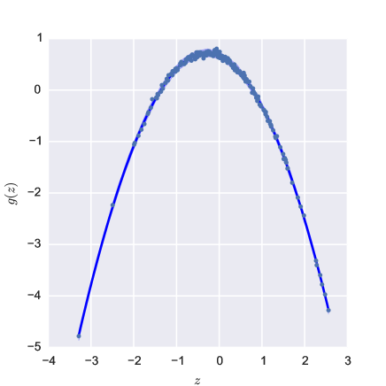
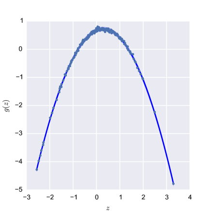
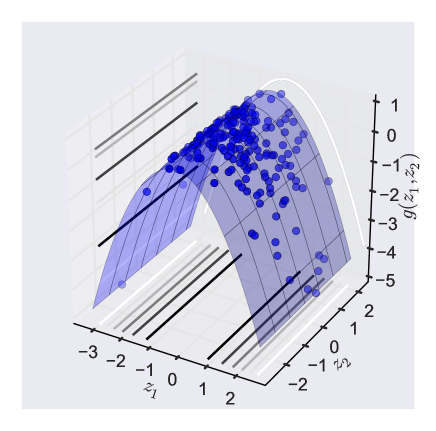
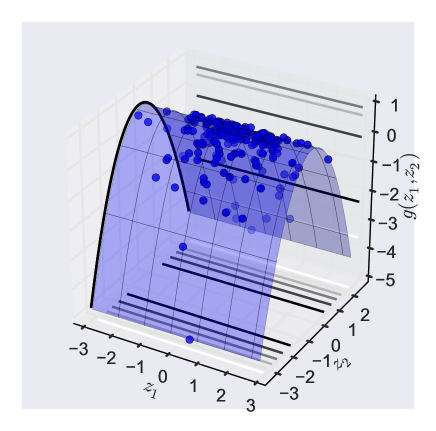
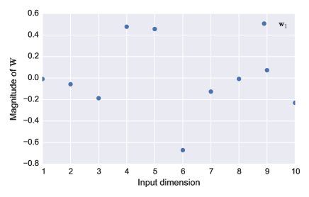
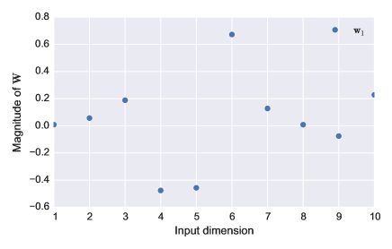
Figure 1: Synthetic example $d=1$. The left and the right columns correspond to results obtained with the classic and the gradient-free approach respectively. The first and second rows depict the predictions of each method for the link function assuming a 1D and 2D underlying AS, respectively, along with a scatter plot of the projections of 60 validation inputs vs the validation outputs. The third row visualizes the projection matrix that each method discovers.

In this example the underlying AS is 1D, $d=1$. The projection matrix is:

$$\mathbf{W}=\left(\begin{array}[]{cccccccccc}-0.0091,&-0.0579,&-0.1877,&0.4774,&0.4559,&-0.6714,&-0.1264,&-0.0082,&0.0724,&-0.2308\end{array}\right)^{T},$$ (55)

and the parameters of the link function of Eq. (53) are:

$$\alpha=-0.16113,\bm{\beta}=(\begin{array}[]{c}-0.97483\end{array}),\;\text{and}\;\bm{\Gamma}=(\begin{array}[]{c}-1.66526\end{array}).$$ (56)

We make $N=140$ observations with noise variance $s_{n}^{2}=0.1$. In this first example, we do not make use of the automatic method for the detection of the dimensionality of the AS. Rather, we use the plain vanilla version of both the classic and the gradient-free approaches assuming a 1D or a 2D AS. For validation 60 random input/output pairs, not used in the training process, were generated. Fig. 1 compares the results obtained with both methodologies. The left column corresponds to the classic approach and the right one to the gradient-free approach. The first row, Fig.1(a) and (b), shows the link function learned by each approach assuming $d=1$, along with a $95\%$ prediction interval, and a scatter plot of the validation input/output pairs. The quantitative agreement between the two approaches becomes obvious once one recalls that the representation of Eq. (7) is arbitrary up to permutations and reflections of the reduced dimensions. This is confirmed by looking at the projection matrices discovered by each method, shown in Fig. 1(e) and (f), respectively. It is clearly seen that one is the negative image of the other. In Fig. 1(c) and (d), we depict the link function learned by assuming that $d=2$. Note that, both methods correctly discovered one completely flat direction.

3.1.2 Synthetic response with 2D active subspace

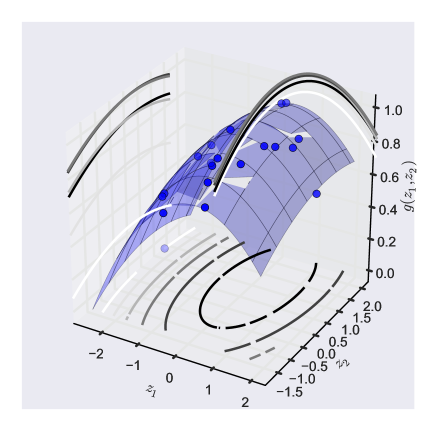
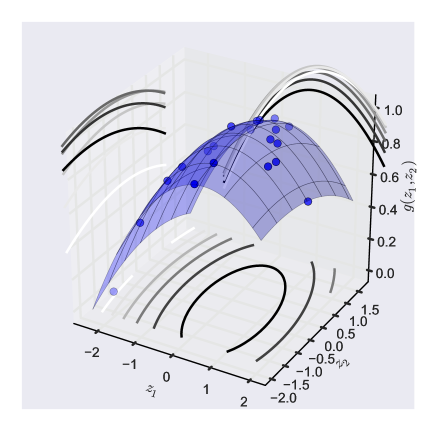
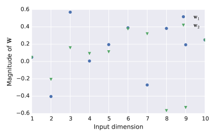
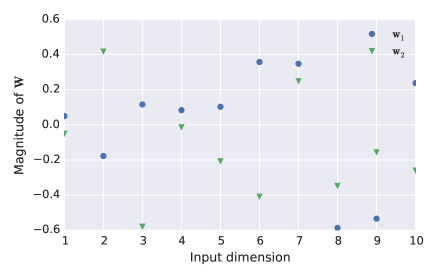
Figure 2: Synthetic example $d=2$. The left and the right columns correspond to results obtained with the classic and the gradient-free approach respectively. The first row depicts the predictions of each method for the link function assuming a 2D underlying AS, along with a scatter plot of the projections of the 60 validation inputs vs the validation outputs. The second row visualizes the projection matrix that each method discovers.

In this example the underlying AS is 2D, $d=2$. The projection matrix is:

$$\mathbf{W}=\left(\begin{array}[]{cccccccccc}0.00840&-0.18426&0.34300&-0.05347&0.08108&0.06556&-0.41219&0.65424&0.48483&0.03966\\ 0.0672&-0.4148&0.4821&0.0755&0.2101&0.5375&0.0781&-0.2002&-0.2912&0.3480\end{array}\right)^{T},$$ (57)

and the parameters of the link function of Eq. (53) are:

$$\alpha=-0.06976,\bm{\beta}=\left(\begin{array}[]{c}0.43759\\ 0.98696041\end{array}\right),\;\text{and}\;\bm{\Gamma}=\left(\begin{array}[]{cc}-0.92567723&-0.38399783\\ -0.41740642&-0.67655046\end{array}\right).$$ (58)

As in Sec. 3.1.1, we make $N=140$ observations with noise variance $s_{n}^{2}=0.1$, We do not make use of Algorithm 4 for the automatic detection of the dimensionality, but rather set $d=2$. Fig. 2 depicts the results. As before, the left column corresponds to the classic approach and the right column to the gradient-free approach. The first row,Fig. 2(a) and (b), shows the learned link function along with a scatter plot of 20 randomly generated input/output pairs. The second row,Fig. 2(c) and (d), shows the learned projection matrices. The quantitative agreement between the two approaches up to permutations and reflections of the AS is also obvious.

3.1.3 Validation of BIC for the identification of the active subspace dimension

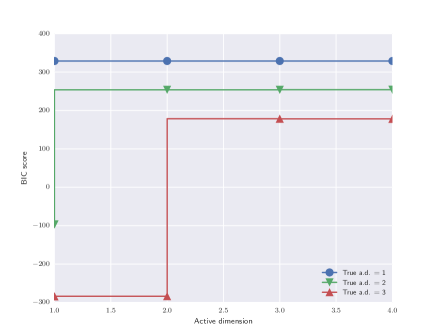
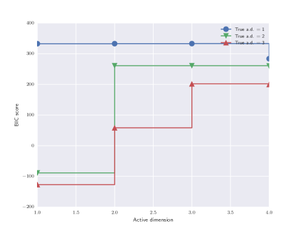
Figure 3: Synthetic example. BIC score as a function of the hypothesized active dimension for classic model (a) and the gradient-free model (b). The different lines correspond to cases with a 1D (blue, true response as in Sec. 3.1.1), 2D (green, true response as in Sec. 3.1.2, and 3D (red, true response as in details on the accompanying website) true AS.

Here, we verify the effectiveness of the BIC, Sec. 2.3.3, to automatically determine the dimensionality of the AS for both the classic and the gradient-free approach. The hypothesis is that the $\operatorname{BIC}_{d}$ becomes flat as a function of $d$ after $d$ exceeds the true AS dimensionality. This is confirmed numerically in Fig. 3 for the cases of a 1D, 2D, and 3D true AS. Note that for the 1D and 2D examples, the observations we used to train the models were the same as in Sec. 3.1.1 and Sec. 3.1.2. For the 3D true AS case also has an underlying response surfaces with randomly generated $\alpha,\bm{\beta},\bm{\Gamma}$, and $\mathbf{W}$. The values used can be found in the accompanying website. As before, we used $N=140$ observations.

3.1.4 Validation of robustness to measurement noise

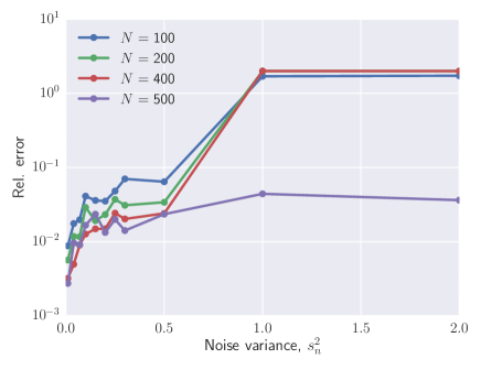
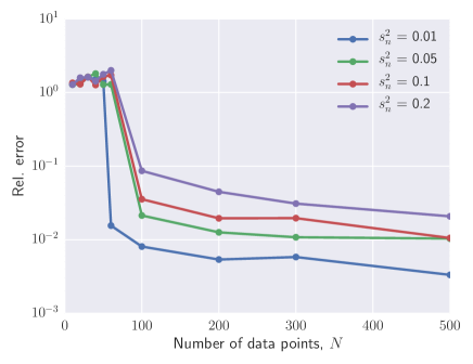
Figure 4: Synthetic example. Robustness of the proposed approach to measurement noise. The figure shows the evolution of the relative error in the determination of the true active subspace as a function of the measurement noise variance (keeping the number of observations constant) (a) and as a function of the number of observations (keeping the measurement noise variance constant (b)).

We conclude this subsection with a study of the robustness of the proposed scheme to measurement noise. To avoid the non-uniqueness issues mentioned earlier, we work with the 10D-input-1D-AS response surface of Sec. 3.1.1. In this case, the arbitrariness can be removed by making sure that the signs of the estimated and the true projection matrix match. We want to quantify the ability of the model to discover the true AS and how this is affected by changes in the measurement noise, $s_{n}$, as well as in the number of available observations $N$. A good measure of this ability is the relative error in the estimation of the projection matrix:

$$\epsilon_{\mbox{rel}}(s_{n},N)=\frac{\|\mathbf{W}(s_{n},N)-\mathbf{W}\|_{F}}{\|\mathbf{W}\|_{F}},$$ (59)

where $\|\cdot\|_{F}$ is the Frobenius norm, $\mathbf{W}(s_{n},N)$ is the estimated projection matrix when $N$ measurements contaminated with zero mean Gaussian noise of variance $s_{n}^{2}$ are used, and $\mathbf{W}$ is the true projection matrix given in Eq. (55). The results of our analysis are presented in Fig. 4. Fig. 4(a) plots the relative error, $\epsilon_{\mbox{rel}}$, as a function of $s_{n}^{2}$ for $N=30,100,200$, and $500$. As expected, we observe that $\epsilon_{\mbox{rel}}$ increases as a function of $s_{n}^{2}$ and that a larger $N$ is required to maintain a given accuracy. Fig. 4(b) plots the relative error, $\epsilon_{\mbox{rel}}$, as a function of $N$ for $s_{n}=0.01,0.05,0.1$ and $0.2$. We note that the method converges to the right answer as $N$ increases, albeit the rate of convergence decreases for higher noise.

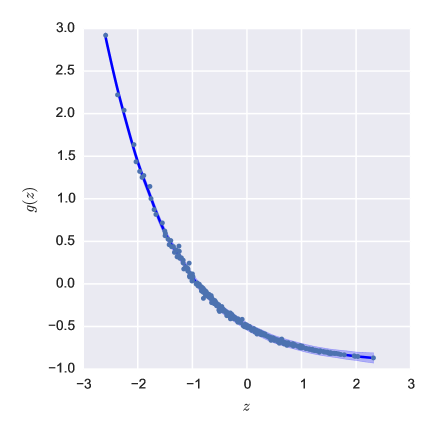
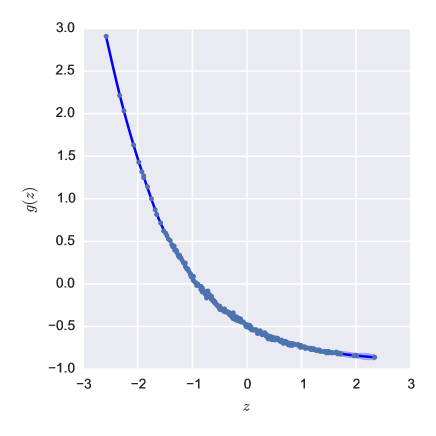
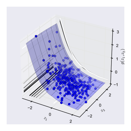
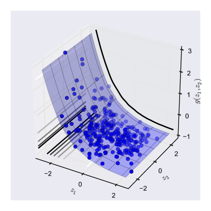
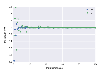
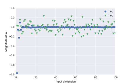
Figure 5: Elliptic PDE, long correlation length ($\ell=1$). The left and the right columns correspond to results obtained with the classic and the gradient-free approach respectively. The first and second rows depict the predictions of each method for the link function assuming a 1D and 2D underlying AS, respectively, along with a scatter plot of the projections of 30 validation inputs vs the validation outputs. The third row visualizes the projection matrix that each method discovers.

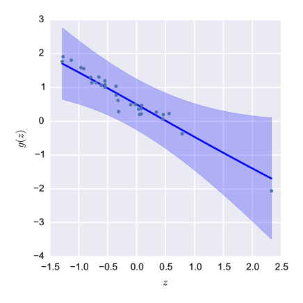
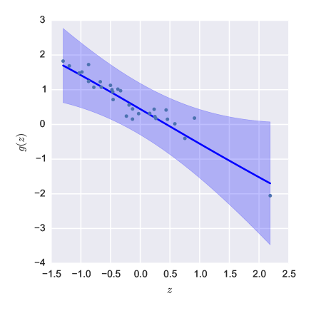
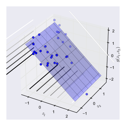
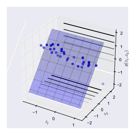
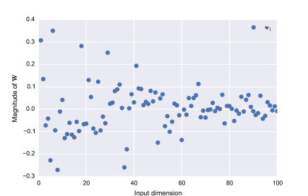
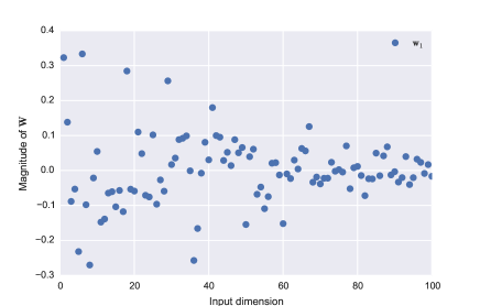
Figure 6: Elliptic PDE, long correlation length ($\ell=0.01$). The left and the right columns correspond to results obtained with the classic and the gradient-free approach respectively. The first and second rows depict the predictions of each method for the link function assuming a 1D and 2D underlying AS, respectively, along with a scatter plot of the projections of 30 validation inputs vs the validation outputs. The third row visualizes the projection matrix that each method discovers.

3.2 Stochastic elliptic partial differential equation

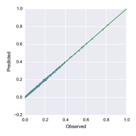
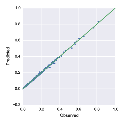
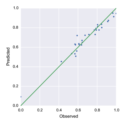
Figure 7: Elliptic PDE. The dots correspond to true observed responses vs predicted ones for 30 validation inputs for the long ($\ell=1$, left) and short ($\ell=0.01$, right) correlation cases. Perfect predictions would fall on the green $45^{\circ}$ line of each subplot. The top row corresponds to the gradient-free approach while the bottom row corresponds to the classic approach.

Consider the elliptic partial differential equation [67]:

$$\nabla\cdot\left(c(\mathbf{s})\nabla u(\mathbf{s})\right)=1,\;\mathbf{s}\in\Omega=[0,1]^{2},$$ (60)

with boundary conditions

$$u(\mathbf{s}) = 0,\ \mathbf{s}\in\Gamma_{1},$$ (61)

$$\nabla u(\mathbf{s})\cdot\mathbf{n} = 0,\ \mathbf{s}\in\Gamma_{2},$$ (62)

where $\Gamma_{1}$ contains the top, bottom and left boundaries, $\Gamma_{2}$ denotes the right boundary of $\Omega$, while $\bm{n}$ is the unit normal vector to the boundary. We assume that the conductivity field is unknown and model its logarithm as a Gaussian random field with an exponential correlation function:

$$C(\mathbf{s},\mathbf{s}^{\prime};\ell)=\exp\left\{-\frac{|s_{1}-s_{1}^{\prime}|+|s_{2}-s_{2}^{\prime}|}{\ell}\right\},$$ (63)

with correlation length $\ell>0$. Using a truncated Karhunen-Loève expansion (KLE) [49], the logarithm of the conductivity can be expressed as:

$$\log\mathbf{c}(\mathbf{s};\mathbf{x}):=\sum_{i=1}^{100}x_{i}\sqrt{\lambda_{i}}\phi_{i}(\mathbf{s}),$$ (64)

where $\lambda_{i}$ and $\phi_{i}(\mathbf{s})$ are the eigenvalues and eigenfunctions of the correlation function, Eq. (63), and $\mathbf{x}$ is a random vector modeled as uniformly distributed on $[-1,1]^{100}$, i.e., $\mathbf{x}\sim\mathcal{U}\left([-1,1]^{100}\right)$. The latter violates the theoretical form of the KLE, but guarantees the existence of a solution to the boundary value problem defined by Eqn.’s (60)-(62) for all $\mathbf{x}$. Given any value for $\mathbf{x}$, the solution of the boundary value problem is $u(\cdot;\mathbf{x})$.

In our analysis, we attempt to learn the following scalar quantity of interest:

$$f(\mathbf{x}):=f[u(\cdot;\mathbf{x})]:=\frac{1}{|\Gamma_{2}|}\int_{\Gamma_{2}}u(\mathbf{s};\mathbf{x})ds,$$ (65)

using both the classic, Sec. 2.2, and the gradient-free approach, Sec. 2.3. We examine two cases exhibiting two different correlation lengths. The first case uses a long correlation length, $\ell=1$, and the second case a short correlation length $\ell=0.01$. In both cases, we use $N=270$ noiseless observations of input-output pairs for training purposes, while setting $30$ aside for validation. The data along with the MATLAB code that generates them, developed by Paul Constantine, can be obtained from https://bitbucket.org/paulcon/active-subspace-methods-in-theory-and-practice/src.

Fig. 5 shows the results we obtain using the long correlation length. The first and second rows of this figure depict the discovered link function under the assumption that $d=1$ and $d=2$, respectively. Note that both methodologies agree on the most important AS dimension, but slightly disagree on the second, albeit relatively flat, dimension. A close examination of the discovered projection matrices, third line of the figure, reveals the following. The most important column of the classic projection matrix, $\mathbf{w}_{1}$, matches with the corresponding column discovered by the gradient free approach. The latter, however, looks like a “noisy” version of the former. This is reasonable if one takes into account that the gradient-free approach uses significantly less information than the classic approach. Finally, we notice that the columns of secondary importance do not match. This discrepancy is unimportant given that the BIC score eventually selects a 1D AS.

Fig. 6 shows the results for the more challenging case of the short correlation length. We present the 1D representation of the link function, as discovered by the classic and the gradient-free approach, in the first row and show the components of the projection matrix estimated by each methodology in the second row. We note that both methodologies show similar 1D active subspace representation of the surrogate. Indeed, this is the most important dimension as the response should be flat along the $2^{nd}$ dimension. We find that the components of projection matrix estimated by both methods are in qualitative agreement for the 1D surrogate. As expected, the BIC score selects the model corresponding to the 1D active subspace as the right model.

Fig. 7 shows the comparison between the prediction on the test inputs and the actual response. The closer the points lie to the green $45^{\circ}$ line, the more accurate the prediction. We make these comparisons for the 1D representation of the link function for both the short and long correlation length cases. It appears that the predictive capabilities of the classic approach are slightly better than the gradient-free approach. A comparison of the RMS error for the predictions by each methodology confirms this although the difference is essentially negligible given its order of magnitude. We tabulate this data in Table 1.

	$\ell=1$	$\ell=0.01$
Classic approach	$1.87\times 10^{-5}$	$3.2\times 10^{-6}$
Gradient-free approach	$2.66\times 10^{-5}$	$3.57\times 10^{-6}$

Table 1: Predictive RMS errors for $\ell=1,0.01$ corresponding to classic and gradient-free methodologies

3.3 Granular Crystals

Granular crystals, or tightly packed lattices of solid particles that deform on contact with each other [102], are strongly nonlinear systems that have attracted significant attention due to their unique dynamics (see, e.g., [103] and references therein). In particular, a one-dimensional uncompressed chain of elastic spherical particles supports the formation and propagation of solitary waves [104], i.e., elastic waves that remain highly localized and coherent while traveling along the chain. This behavior is due to the interplay between nonlinearity and discreteness of the unilateral Herztian contact interaction between the particles in the system. Over the last two decades, extensive experimental, computational and theoretical research has been conducted to advance the understanding of theses systems. For example, experimental techniques have been developed to measured the temporal evolution of the solitary wave [105, 106, 107], and dissipative [108, 109, 110], plastic [111] and nonlocal [112] deformation effects between particles have been included in simulations. However, a systematic and thorough uncertainty analysis of theses systems remains elusive, mainly due to the curse of dimensionality. It is worth noting that the high localization of this elastic waves suggests the use of an AS approach, specifically a gradient-free approach due to the lack of gradient information. We present the mathematics of the problem next.

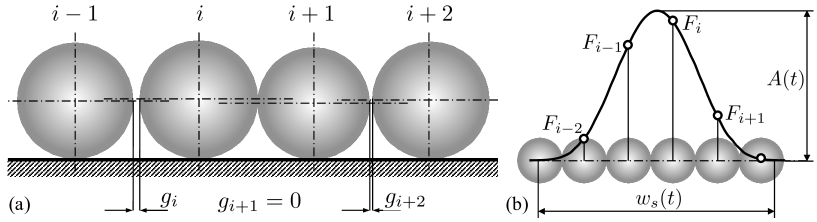
Figure 8: One-dimensional granular crystal. (a) Initial equilibrium position of spherical particles in contact with a horizontal flat rigid surface under the action of gravity. Particles are separated from point contact by horizontal positive gaps $g_{i}$. (b) Traveling solitary wave with amplitud $A(t)$ and width $w_{s}(t)$ as defined by averaged compressive forces $\tilde{F}_{i}(t)$ acting on particles $i$.

Consider a one-dimensional chain of $n_{p}\ (=47)$ spherical particles whose displacements from the initial equilibrium positions are described by the position matrix $\mathbf{q}=\left(\mathbf{q}_{1},\mathbf{q}_{2},\cdots,\mathbf{q}_{n_{p}}\right)$ with $\mathbf{q}_{i}\in\mathbb{R}^{3}$. The equilibrium position is such that particles are in contact with a horizontal flat rigid surface under the action of gravity. In addition, a positive gap $g_{i}$ may exist between $i$-th and $i-1$-th particles—$g_{1}$ corresponds to the gap between the first particle and a rigid back wall. A gap equal to zero corresponds to point contact. Each bead has a radius $R_{i}$ and Young’s modulus $E_{i}$. The density of the particles is a constant $\rho=7,900\mbox{kg}/\mbox{m}^{3}$ and the mass of each particle is $m_{i}=\rho\frac{4}{3}\pi R_{i}^{3}$. A solitary wave forms and propagates through the one-dimensional granular crystal after the $n_{p}$-th particle strikes the chain with velocity $v_{s}$. Therefore, all the parameters of the system are:

$$\mathbf{x}=\left(R_{1},R_{2},\dots,R_{n_{p}},E_{1},E_{2},\dots,E_{n_{p}},g_{1},g_{2},\dots,g_{n_{p}},v_{s}\right)\in\mathbb{R}^{3n_{p}+1}.$$ (66)

In the present effort, we consider the two cases where: a) the particles are in point contact with each other and thus, the system is completely parameterized by the particle radii, the Young’s moduli and the striker velocity:

$$\mathbf{x}=\left(R_{1},R_{2},\dots,R_{n_{p}},E_{1},E_{2},\dots,E_{n_{p}},v_{s}\right)\in\mathbb{R}^{2n_{p}+1},$$ (67)

and b) where the particles are separated by small gaps and thus, the system is parameterized by $\mathbf{x}$ as defined in Eq. (66). The displacement vector satisfies Newton’s law of motion:

$$m_{i}(\mathbf{x})\ddot{\mathbf{q}}_{i}=\mathbf{F}^{\mathrm{H}}_{i-1,i}\left(\mathbf{q};\mathbf{x}\right)+\mathbf{F}^{\mathrm{H}}_{i+1,i}\left(\mathbf{q};\mathbf{x}\right),$$ (68)

where $\mathbf{F}^{\mathrm{H}}_{k,i}\left(\mathbf{q};\mathbf{x}\right)$ is the unilateral Hertzian contact force between particle $k$ and $i$ [102, 106, 110]. The initial conditions are:

$$\mathbf{q}_{i}(0) = (0,0,0),$$

$$\dot{\mathbf{q}}_{i}(0) = (0,0,0),\;\forall\;i=\{1,2,3,\cdots,n_{p}-1\},$$

$$\dot{\mathbf{q}}_{n_{p}}(0) = (-v_{s},0,0).$$

Let $\mathbf{q}(t;\mathbf{x})$ be the solution to this initial value problem. We are interested in characterizing the properties of the solitary wave propagated through the granular crystal. To this end, we will be observing an average of the absolute value of the horizontal component of the two unilateral Hertzian contact forces acting on each particle as a function of time for a given set of parameters $\mathbf{x}$ [105],

$$\tilde{F}_{i}\left(t;\mathbf{x}\right)\equiv\dfrac{1}{2}\left[\mathbf{F}^{\mathrm{H}}_{i-1,i}\left(\mathbf{q}\left(t;\mathbf{x}\right);\mathbf{x}\right)+\mathbf{F}^{\mathrm{H}}_{i,i+1}\left(\mathbf{q}\left(t;\mathbf{x}\right);\mathbf{x}\right)\right]\cdot(1,0,0).$$ (69)

That is, for each $\mathbf{x}$, we obtain, by integrating the equations of motion, the force at a finite number of timesteps, $0=t_{1}<\dots<t_{n_{t}}$, $n_{t}=6252$. The output, for each $\mathbf{x}$, forms a matrix $\tilde{\mathbf{F}}(\mathbf{x}):=\{\tilde{F}_{i}(t_{j};\mathbf{x}):i=1,\dots,n_{p},j=1,\dots,n_{t}\}$. The dimensionality of the $\tilde{\mathbf{F}}(\mathbf{x})$ is $n_{p}\times n_{t}$. The time step at which the maximum force is observed as the solitary wave passes over particle $i$:

$$j_{i}^{*}(\mathbf{x})=\arg\max_{j}\tilde{F}_{ij}(\mathbf{x}).$$ (70)

In order to characterize the behavior of the soliton as it propagates over the particle chain, we look at three properties of the soliton as it stands over any given particle - the amplitude $(A_{i})$, the time of flight $(t_{\mbox{flight}})$ and full width at half maximum $(f_{\mbox{h}})$. The amplitude of the soliton as it passes over the particle is obtained as follows:

$$A_{i}(\mathbf{x})=\tilde{F}_{ij_{i}^{*}(\mathbf{x})}(\mathbf{x}).$$ (71)

Then we extract the width, $f_{\mbox{h}}$, as follows:

$$f_{\mbox{h},i}(\mathbf{x})=0.364\ w_{s}(j_{i}^{*}(\mathbf{x})),$$ (72)

where $w_{s}(t)$ is the width of the soliton at any given instance of time $t$. Finally, we extract the time of flight of the soliton as it passes over particle $i$:

$$t_{\mbox{flight},i}(\mathbf{x})=t_{j_{i}^{*}(\mathbf{x})}.$$ (73)

We study these properties of the soliton as it travels over the $20^{th}$ and $30^{th}$ particles. Let us denote these quantities as $y_{1}=t_{\mbox{flight},20},y_{2}=A_{20},y_{3}=f_{\mbox{h},20},y_{4}=t_{\mbox{flight},30},y_{5}=A_{20},y_{6}=f_{\mbox{h},20}$. We repeat this entire process for $1000$ samples of $\mathbf{x}$ and construct the output vectors $\mathbf{y}_{1},\mathbf{y}_{2},\mathbf{y}_{3},\mathbf{y}_{4},\mathbf{y}_{5}$ and $\mathbf{y}_{6}$ which we define as $\mathbf{y}_{i}=\{y_{i}^{(1)},\dots,y_{i}^{(1000)}\}$ such that $\mathbf{y}_{i}\in\mathbb{R}^{1000}$. The input in each simulation is the vector of parameters shown in Eq. (66) and Eq. (67) for cases with and without inter particle gaps respectively. Thus with 1000 of these input vectors we contruct the input design matrices $\mathbf{X}_{1}\in\mathbb{R}^{1000\times 2n_{p}+1}$ and $\mathbf{X}_{2}\in\mathbb{R}^{1000\times 3n_{p}+1}$ for the cases with and without point contacts, respectively.

We now proceed to apply our proposed gradient-free AS approach to build a cheap-to-evaluate surrogate for propagating uncertainty through this system. We train the model on 1000 observations with inputs sampled using a Latin Hypercube design within the range $(180\mbox{GPa},220\mbox{GPa})$ for Young’s moduli input, $(8.57\mbox{mm},10.47\mbox{mm})$ for radii input, $(1.125\mbox{m/s},1.375\mbox{m/s})$ for impact velocities input and gaps $g_{i}$ such that 90% of the time $g_{i}=0$ (i.e. there is no gap between the $i-1^{th}$ and $i^{th}$ particles) and the remaining 10% of the time there $g_{i}=0.001R_{i}$. Note that we construct a different AS for each one of the cases. We use 100 out-of-sample data to test the predictive accuracy of the surrogate. We consider all possible combinations of data-sets $\mathcal{D}_{j}=\{\mathbf{X}_{i},\mathbf{y}_{j}\},\ \ \forall i\in\{1,2\},\ \forall j\in\{1,2,3,4\}$, and build the corresponding surrogates.

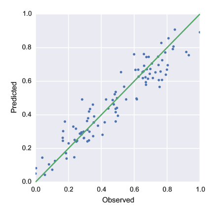
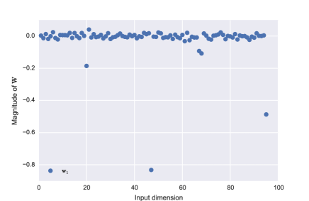
Figure 9: One-dimensional granular crystal without gaps - amplitude of the soliton over the $20^{th}$ particle. The first plot shows the response surface in the active subspace. the second plot depicts the test observations vs model prediction plot. The final plot depicts the components of the projection matrix.

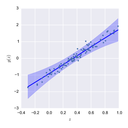
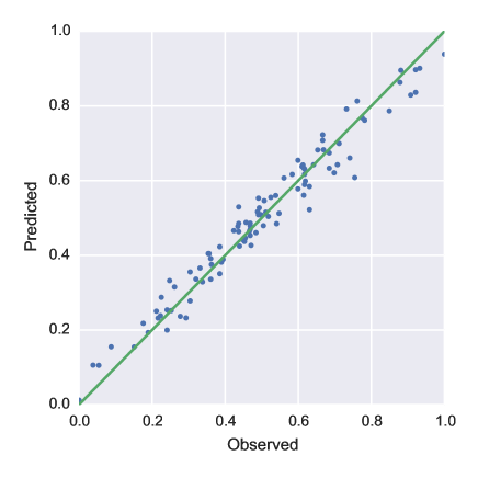
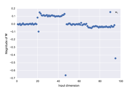
Figure 10: One-dimensional granular crystal without gaps - time of flight of the soliton over the $20^{th}$ particle. The first plot shows the response surface in the active subspace. the second plot depicts the test observations vs model prediction plot. The final plot depicts the components of the projection matrix.

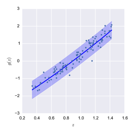
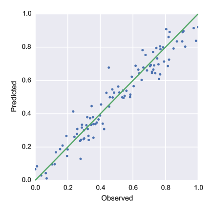
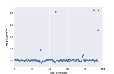
Figure 11: One-dimensional granular crystal without gaps - amplitude of the soliton over the $30^{th}$ particle. The first plot shows the response surface in the active subspace. the second plot depicts the test observations vs model prediction plot. The final plot depicts the components of the projection matrix.

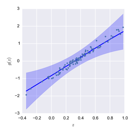
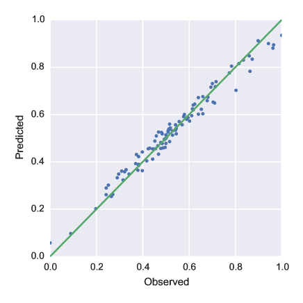
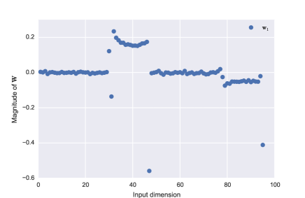
Figure 12: One-dimensional granular crystal without gaps - time of flight of the soliton over the $30^{th}$ particle. The first plot shows the response surface in the active subspace. the second plot depicts the test observations vs model prediction plot. The final plot depicts the components of the projection matrix.

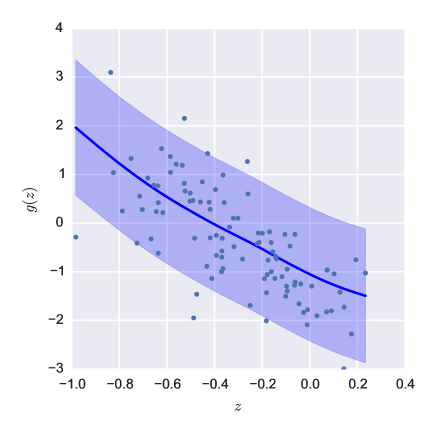
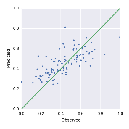
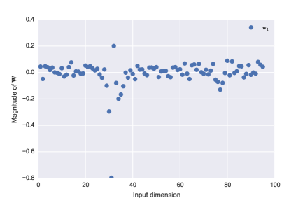
Figure 13: One-dimensional granular crystal without gaps - full width at half maximum of the soliton over the $30^{th}$ particle. The first plot shows the response surface in the active subspace. the second plot depicts the test observations vs model prediction plot. The final plot depicts the components of the projection matrix.

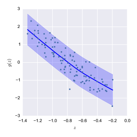
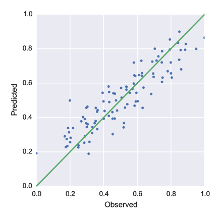
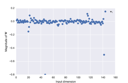
Figure 14: One-dimensional granular crystal with gaps - amplitude of the soliton over the $20^{th}$ particle. The first plot shows the response surface in the active subspace. the second plot depicts the test observations vs model prediction plot. The final plot depicts the components of the projection matrix.

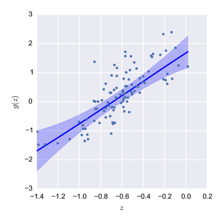
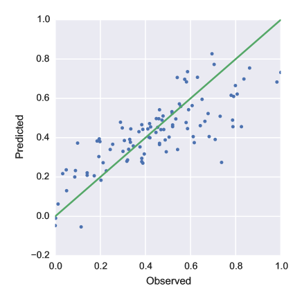
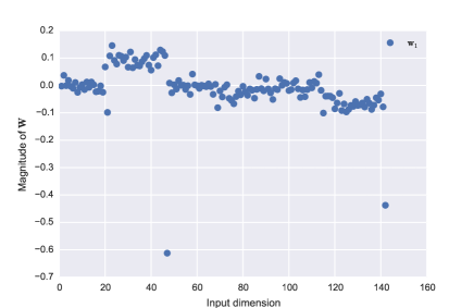
Figure 15: One-dimensional granular crystal with gaps - time of flight of the soliton over the $20^{th}$ particle. The first plot shows the response surface in the active subspace. the second plot depicts the test observations vs model prediction plot. The final plot depicts the components of the projection matrix.

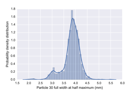
Figure 16: One-dimensional granular crystal with gaps - histogram of the observed full width outputs for the $30^{th}$ particle corresponding to the gaps input case.

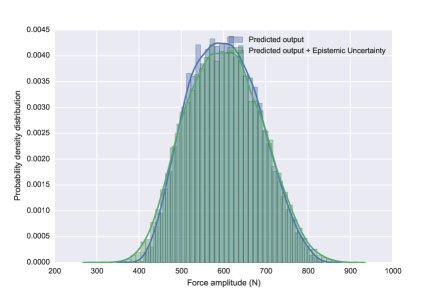
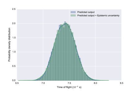
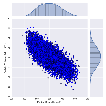
Figure 17: One-dimensional granular crystal without gaps - propagating the uncertainty by assigning a uniform distribution to the inputs. (a) Marginal distribution of the amplitude of the soliton over the $20^{th}$ particle; (b) Marginal distribution of the time of flight of the soliton over the $20^{th}$ particle; (c) Joint distribution of the amplitude and time of flight of the soliton over the $20^{th}$ particle. For the plots corresponding to the marginal distributions the blue histogram and curve represents the mean predictions of the surrogate while the green histogram and curve represents the mean predictions added with Gaussian noise of variance equal to the variance of the GP surrogate. The difference between the blue and green curves is a measure of the associated epistemic uncertainty in the output QoI.

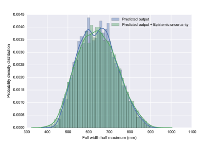
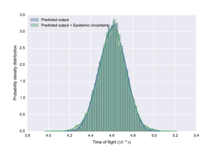
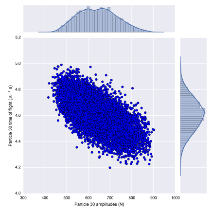
Figure 18: One-dimensional granular crystal without gaps - propagating the uncertainty by assigning a uniform distribution to the inputs. (a) Marginal distribution of the amplitude of the soliton over the $30^{th}$ particle; (b) Marginal distribution of the time of flight of the soliton over the $30^{th}$ particle; (c) Joint distribution of the amplitude and time of flight of the soliton over the $30^{th}$ particle. For the plots corresponding to the marginal distributions the blue histogram and curve represents the mean predictions of the surrogate while the green histogram and curve represents the mean predictions added with Gaussian noise of variance equal to the variance of the GP surrogate. The difference between the blue and green curves is a measure of the associated epistemic uncertainty in the output QoI.

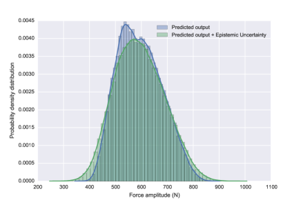
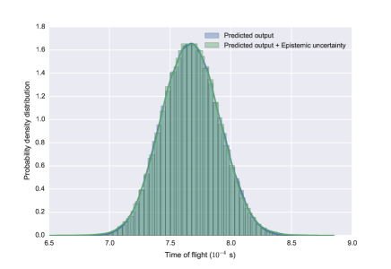
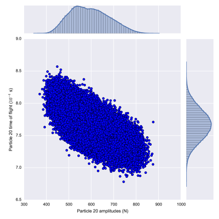
Figure 19: One-dimensional granular crystal with gaps - propagating the uncertainty by assigning a uniform distribution to the inputs. (a) Marginal distribution of the amplitude of the soliton over the $20^{th}$ particle; (b) Marginal distribution of the time of flight of the soliton over the $20^{th}$ particle; (c) Joint distribution of the amplitude and time of flight of the soliton over the $20^{th}$ particle. For the plots corresponding to the marginal distributions the blue histogram and curve represents the mean predictions of the surrogate while the green histogram and curve represents the mean predictions added with Gaussian noise of variance equal to the variance of the GP surrogate. The difference between the blue and green curves is a measure of the associated epistemic uncertainty in the output QoI.

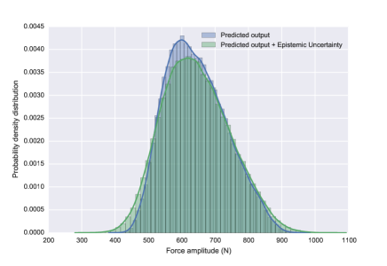
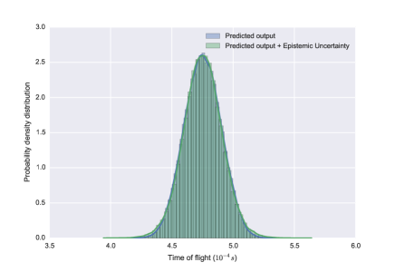
Figure 20: One-dimensional granular crystal with gaps - propagating the uncertainty by assigning a uniform distribution to the inputs.. (a) Marginal distribution of the amplitude of the soliton over the $30^{th}$ particle; (b) Marginal distribution of the time of flight of the soliton over the $30^{th}$ particle; (c) Joint distribution of the amplitude of the soliton over the $30^{th}$ particle and the time of flight of the soliton over the $30^{th}$ particles. For the plots corresponding to the marginal distributions the blue histogram and curve represents the mean predictions of the surrogate while the green histogram and curve represents the mean predictions added with Gaussian noise of variance equal to the variance of the GP surrogate. The difference between the blue and green curves is a measure of the associated epistemic uncertainty in the output QoI.

3.3.1 Results

The GP surrogate was trained using 1,000 data samples and validated using a further 100 samples. It is observed that most of the stochasticity of this high dimensional problem is exhibited on a one dimensional active subspace. We present plots of the AS representation of the link function, projection matrix and predictions vs observations plots for the cases noted above. Note that the underlying response surfaces obtained are approximately linear. There is very good agreement between the training data-set output predictions as compared to the actual training set outputs. In all the cases that we just demonstrated, we observe the localized nature of the soliton.

We first discuss the case when the particles are in point contact i.e. the input design matrix is $\mathbf{X}_{1}$. From plots corresponding to the soliton amplitude over particles 20 and 30 , shown in Fig. 9 and 11 we observe that the projection matrix has zero entries for most components except those corresponding to the radius and Young’s modulus of the respective particle under observation and the particle at the striker end. Likewise, from plots corresponding to the case of the time of flight outputs over the respective particles, in Fig. 10 and Fig. 12, we observe that the entries of the projection matrix are approximately zero for components corresponding to the radii and Young’s moduli of the particles before the particle under observation. We also note that the time of flight depends more on the particle radii than the particle Young’s moduli, as evidenced by the larger weights assigned to the radii terms in the projection matrix. Finally, we present the plots corresponding to the full width of the soliton as it stands over particle 30 in Fig. 13. The change in the BIC score from the 1st active dimension to the 2nd active dimension is insignificant and as such, suggests that we should be looking at a one dimensional active subspace. We note that the link function shows slight non-linearity. The large non-zero weights are associated with the radii terms in and around the $30^{th}$ particle. We believe that the remaining components of the projection matrix should have been closer to zero and the likely cause of this not being case would be that the optimization routine gets stuck in a local minima despite several restarts of the algorithm from random initial points.

We now discuss the more challenging case when the particles are separated by gaps i.e. when the input design matrix is $\mathbf{X}_{2}$. In Fig. 14, we show the plots corresponding to the case of soliton amplitude over the $20^{th}$ particle. Looking at the projection matrix, we observe that it shows a similar trend to the corresponding matrix when we considered point contact inputs, i.e., the magnitude of most of the components of the projection matrix are approximately zero and significantly large weights are associated with the radius of the $20^{th}$ particle and the striker velocity. From Fig. 15 we observe that the components of the projection matrix, when looking at the time of flight of the soliton over the $20^{th}$ particle. We note that there are non-zero components of the projection matrix on a few terms corresponding to the radii and Young’s moduli in and around the $20^{th}$ particle, with the weights being higher on the radii as opposed to the Young’s moduli terms. Our method was unable to converge to an active subspace for the case of the full width output and as such we don’t present it here. In Fig. 16, we present the histogram of the observed full width output for the $30^{th}$ particle and find that it is bimodal. This suggests the presence of a discontinuity in the response which can be resolved, given sufficient data and clustering of the data into appropriate batches. Overall, we observe that the trends in the link function and the projection matrix for different outputs corresponding to the two different input cases are similar. It is not surprising that the results look significantly better when we consider the case of point contact between the particles as opposed to the case where we consider the case where gaps exist between the particles. This is because in the former case, the GP surrogate has to learn fewer parameters from the same limited quantity of data. Given the very dimensional nature of the associated optimization problem in the case of the gaps inputs, it is also likely that the optimization algorithm gets stuck in a local minima despite several restarts of the algorithm from random initial starting points. We do not present plots for the link function and projection matrices for the soliton properties corresponding to the $30^{th}$ particle in the gaps input case since they follow trends similar to what has been discussed so far.

3.3.2 Uncertainty Quantification

Having built a cheap-to-evaluate response surface, we can tackle the uncertainty propagation problem in an efficient manner. We assign a uniform distribution to the inputs. Then, we sample 10,000 observations of the input from this distribution and use the surrogate to generate predictions for the time of flight and amplitude of the soliton as it passes over the respective particles. Finally, we plot the marginal and joint distributions of some of the outputs as shown in Fig. 17, 18, 19 and 20. For each of the marginal distribution plots, we also show the associated epistemic uncertainty. We observe that for a uniform distribution over the inputs, the outputs look approximately normal.

4 Conclusions

We have developed a gradient-free approach to active subspace (AS) discovery and exploitation suitable for dealing with noisy outputs. We did so by developing a novel Gaussian process regression model with built-in dimensionality reduction. Specifically we represented the AS as an orthogonal projection matrix that constitutes a hyper-parameter of the covariance function to be estimated from the data by maximizing the likelihood. Towards this end, we devised a two-step optimization procedure that ensures the orthogonality of the projection matrix by exploiting recent results on the description of the Stiefel manifolds. An addendum of the probabilistic approach is the ability to use the Bayesian information criterion (BIC) to automatically select the dimensionality of the AS. We validated our method using both synthetic examples with known AS and by comparing directly to the classic gradient-based AS approach. Finally, we used our method to study the effect of geometric and material uncertainties in force waves propagated through granular crystals.

This work is a first step towards a fully Bayesian AS-based surrogate, a persistent theme of our current research plans. As argued in [38], Bayesian surrogates should be capable of quantifying all the epistemic uncertainty induced by limited data, since quantification of this epistemic uncertainty is the key to deriving problem-specific information acquisition policies, i.e., rules for deciding where to sample the model next in order to obtain the maximum amount of information towards a specific task. A fully Bayesian treatment requires the specification of priors for all the hyper-parameters of the covariance function and the derivation of Markov Chain Monte Carlo (MCMC) schemes to sample from the posterior of the model. The big challenge is the construction of proposals that force $\mathbf{W}$ to remain on the Stiefel manifold, which could be achieved, for example, by modifying the Riemann manifold Hamiltonian MC of [113]. Such approaches would open the way for more robust AS dimensionality selection, e.g., by reversible-jump MC [114] or by directly computing the model evidence.

Many physical models do not have an AS. They may have, however, a non-linear low-dimensional manifold exhibiting maximal response variability. Assuming that this low-dimensional manifold is a Riemann manifold, i.e., locally isomorphic to a Eucledian space, a potential approach would be to consider mixtures of the model proposed in this work. To this end, the results of [37] on infinite mixtures of GP’s could be leveraged. The latter is also a subject of on-going research.

Ilias Bilionis and Marcial Gonzalez acknowledge the startup support provided by the School of Mechanical Engineering at Purdue University.

References

- [1] Ralph C. Smith. Uncertainty quantification : theory, implementation, and applications. Philadelphia : SIAM, 2014.
- [2] W. Chen. Efficient uncertainty analysis methods for multidisciplinary robust design. AIAA Journal, 40(3):545–552, 2002.
- [3] F. D’Auria and G. M. Galassi. Outline of the uncertainty methodology based on accuracy extrapolation. Nuclear Technology, 109(1), 1995.
- [4] Wl Oberkampf, Jc Helton, Ca Joslyn, Sf Wojtkiewicz, and S. Ferson. Challenge problems: uncertainty in system response given uncertain parameters. Reliab. Eng. Syst. Saf., 85(1-3):11–19, 2004.
- [5] Jun S. Liu. Monte Carlo strategies in scientific computing. New York : Springer, New York, 2001.
- [6] Christian P. Robert. Monte Carlo statistical methods. New York : Springer, New York, 2nd ed.. edition, 2004.
- [7] W. J. Morokoff and R. E. Caflisch. Quasi-Monte Carlo integration. Journal of Computational Physics, 122(2):218–230, 1995.
- [8] A. Barth, C. Schwab, and N. Zollinger. Multi-level Monte Carlo finite element method for elliptic PDEs with stochastic coefficients. Numerische Mathematik, 119(1):123–161, 2011.
- [9] F. Y. Kuo, C. Schwab, and I. H. Sloan. Quasi-Monte Carlo finite element methods for a class of elliptic partial differential equations with random coefficients. SIAM Journal on Numerical Analysis, 50(6):3351–3374, 2012.
- [10] A Tarantola. Inverse problem theory and methods for model parameter estimation. SIAM, 2004.
- [11] I. Bilionis, B. A. Drewniak, and E. M. Constantinescu. Crop physiology calibration in the clm. Geoscientific Model Development, 8(4):1071–1083, 2015. GMD http://www.geosci-model-dev.net/8/1071/2015/gmd-8-1071-2015.pdf.
- [12] J. C. Spall. Introduction to stochastic optimization. Wiley, 2003.
- [13] I. Bilionis and P. S. Koutsourelakis. Free energy computations by minimization of kullback-leibler divergence: An efficient adaptive biasing potential method for sparse representations. Journal of Computational Physics, 231(9):3849–3870, 2012.
- [14] I. Bilionis and N. Zabaras. A stochastic optimization approach to coarse-graining using a relative-entropy framework. Journal of Chemical Physics, 138(4), 2013.
- [15] A. O’Hagan. Monte carlo is fundamentally unsound. Statistician, 36(2-3):247–249, 1987. J4389 Times Cited:13 Cited References Count:3.
- [16] Dongbin Xiu and George Em Karniadakis. The wiener–askey polynomial chaos for stochastic differential equations. SIAM Journal on Scientific Computing, 24(2):619–644, 2002.
- [17] Db Xiu and Js Hesthaven. High-order collocation methods for differential equations with random inputs. SIAM J. Sci. Comput., 27(3):1118–1139, 2005.
- [18] Db Xiu. Efficient collocational approach for parametric uncertaintyrtainty analysis. Communications In Computational Physics, 2(2):293–309, 2007.
- [19] Babuška Ivo, Nobile Fabio, and Tempone Raúl. A stochastic collocation method for elliptic partial differential equations with random input data. SIAM Review, 52:317, 2010.
- [20] Sethuraman Sankaran and Alison L. Marsden. A stochastic collocation method for uncertainty quantification and propagation in cardiovascular simulations. Journal of biomechanical engineering, 133(3):031001, 2011.
- [21] H.-M. Gutmann. A radial basis function method for global optimization. Journal of Global Optimization, 19(3):201–227, 2001.
- [22] R. G. Regis and Ca Shoemaker. Constrained global optimization of expensive black box functions using radial basis functions. J. Glob. Optim., 31(1):153–171, 2005.
- [23] Ilias Bilionis and Nicholas Zabaras. Multidimensional adaptive relevance vector machines for uncertainty quantification. SIAM Journal on Scientific Computing, 34(6):B881–B908, 2012.
- [24] Xiang Ma and Nicholas Zabaras. An adaptive hierarchical sparse grid collocation algorithm for the solution of stochastic differential equations. Journal of Computational Physics, 228(8):3084 – 3113, 2009.
- [25] C. Currin, T. Mitchell, M. Morris, and D. Ylvisaker. A bayesian approach to the design and analysis of computer experiments. Report, Oak Ridge Laboratory, 1988.
- [26] J. Sacks, W. J. Welch, T. Mitchell, and H. P. Wynn. Design and analysis of computer experiments. Statistical Science, 4(4):409–423, 1989.
- [27] C. Currin, T. Mitchell, M. Morris, and D. Ylvisaker. Bayesian prediction of deterministic functions, with applications to the design and analysis of computer experiments. Journal of the American Statistical Association, 86(416):953–963, 1991.
- [28] I. Bilionis and N. Zabaras. Multi-output local gaussian process regression: Applications to uncertainty quantification. J. Comput. Phys., 231(17):5718–5746, 2012.
- [29] B. A. Lockwood and M. Anitescu. Gradient-enhanced universal kriging for uncertainty propagation. Nuclear Science And Engineering, 170(2):168–195, 2012.
- [30] I. Bilionis, N. Zabaras, B. A. Konomi, and G. Lin. Multi-output separable gaussian process: Towards an efficient, fully bayesian paradigm for uncertainty quantification. Journal Of Computational Physics, 241:212–239, 2013.
- [31] I. Bilionis and N. Zabaras. Solution of inverse problems with limited forward solver evaluations: a bayesian perspective. Inverse Problems, 30(1), 2014.
- [32] C. E. Rasmussen and C. K. I. Williams. Gaussian Processes for Machine Learning. MIT press, Cambridge, 2005.
- [33] A. O’Hagan. Bayes-hermite quadrature. Journal of Statistical Planning and Inference, 29(3):245–260, 1991.
- [34] A. O’Hagan, M. C. Kennedy, and J. E. Oakley. Uncertainty analysis and other inference tools for complex computer codes. Bayesian Statistics 6, pages 503–524, 1999.
- [35] J. Oakley and A. O’Hagan. Bayesian inference for the uncertainty distribution of computer model outputs. Biometrika, 89(4):769–784, 2002.
- [36] J. E. Oakley and A. O’Hagan. Probabilistic sensitivity analysis of complex models: a bayesian approach. Journal of the Royal Statistical Society Series B-Statistical Methodology, 66:751–769, 2004.
- [37] P. Chen, N. Zabaras, and I. Bilionis. Uncertainty propagation using infinite mixture of gaussian processes and variational bayesian inference. Journal of Computational Physics, 284:291–333, 2015.
- [38] I. Bilionis and N. Zabaras. Bayesian uncertainty propagation using Gaussian processes. Springer, 2016 (accepted).
- [39] D. J. C. Mackay. Bayesian interpolation. Neural Computation, 4(3):415–447, 1992.
- [40] P. Balaprakash, R. B. Gramacy, and S. M. Wild. Active-learning-based surrogate models for empirical performance tuning, 2013.
- [41] D. R. Jones. A taxonomy of global optimization methods based on response surfaces. Journal of Global Optimization, 21(4):345–383, 2001.
- [42] M. Emmerich, N. Beume, and B. Naujoks. An emo algorithm using the hypervolume measure as selection criterion. Evolutionary Multi-Criterion Optimization, 3410:62–76, 2005.
- [43] Y. Bengio, O. Delalleau, and N. Le Roux. The curse of highly variable functions for local kernel machines. In Neural Information Processing Systems, 2005.
- [44] R. Bellman. Dynamic programming and lagrange multipliers. Proceedings of the National Academy of Sciences of the United States of America, 42(10):767–769, 1956.
- [45] Saltelli A., Ratto M., Andres T., Campolongo F., Cariboni J., and D.and Saisana M.and Tarantola S. Gatelli. Global sensitivity analysis the primer. Chichester, England ; Hoboken, NJ : John Wiley, Chichester, England ; Hoboken, NJ, 2008.
- [46] C. Smith, Ralph. Uncertainty quantification: Theory, implementation, and applications. SIAM, 2014.
- [47] R. M. Neal. Bayesian learning for neural networks., volume 118. Springer, New York, 1996.
- [48] R. M. Neal. Assessing relevance determination methods using DELVE, pages 97–129. Springer-Verlag, 1998.
- [49] Roger Ghanem and P. D. Spanos. Stochastic finite elements: a spectral approach. Dover Publications, Minneola, N.Y., 2003.
- [50] Karl Pearson. Liii. on lines and planes of closest fit to systems of points in space. Philosophical Magazine Series 6, 2(11):559–572, 1901.
- [51] X. Ma and N. Zabaras. Kernel principal component analysis for stochastic input model generation. Journal of Computational Physics, 230(19):7311–7331, 2011.
- [52] H. Rabitz and O. F. Alis. General foundations of high-dimensional model representations. Journal of Mathematical Chemistry, 25(2-3):197–233, 1999.
- [53] O. F. Alis and H. Rabitz. Efficient implementation of high dimensional model representations. Journal of Mathematical Chemistry, 29(2):127–142, 2001.
- [54] G. Y. Li, C. Rosenthal, and H. Rabitz. High dimensional model representations. Journal of Physical Chemistry A, 105(33):7765–7777, 2001.
- [55] G. Y. Li, S. W. Wang, C. Rosenthal, and H. Rabitz. High dimensional model representations generated from low dimensional data samples. 1. mp-cut-hdmr. Journal of Mathematical Chemistry, 30(1):1–30, 2001.
- [56] R. Chowdhury, B. N. Rao, and A. M. Prasad. High-dimensional model representation for structural reliability analysis. Communications in Numerical Methods in Engineering, 25(4):301–337, 2009.
- [57] X. Ma and N. Zabaras. An adaptive high-dimensional stochastic model representation technique for the solution of stochastic partial differential equations. Journal of Computational Physics, 229(10):3884–3915, 2010.
- [58] J. Wei, G. Lin, L. J. Jiang, and Y. Efendiev. Analysis of variance-based mixed multiscale finite element method and applications in stochastic two-phase flows. International Journal for Uncertainty Quantification, 4(6):455–477, 2014.
- [59] Z. W. Zhang, X. Hu, T. Y. Hou, G. Lin, and M. K. Yan. An adaptive anova-based data-driven stochastic method for elliptic pdes with random coefficient. Communications in Computational Physics, 16(3):571–598, 2014.
- [60] T. A. Plate. Accuracy versus interpretability in flexible modeling: Implementing a tradeoff using gaussian process models. Behaviormetrika, 26:29–50, 1999.
- [61] C. G. Kaufman and S. R. Sain. Bayesian functional ANOVA modeling using Gaussian process prior distributions. Bayesian Analysis, 5(1):123–149, 2010.
- [62] N. Durrande, D. Ginsbourger, and O. Roustant. Additive covariance kernels for high-dimensional Gaussian process modeling. arXiv:1111.6233, 2011.
- [63] D. Duvenaud, H. Nickisch, and C. E. Rasmussen. Additive Gaussian processes. In Advances in Neural Information Processing Systems 24, pages 226–234.
- [64] E. Gliboa, Y. Saatci, and J. Cunningham. Scaling multidimensional inference for structured Gaussian processes. In 30th International Conference on Machine Learning.
- [65] X. Nguyen and A. E. Gelfand. Bayesian nonparametric modeling for functional analysis of variance. Annals of the Institute of Statistical Mathematics, 66(3):495–526, 2014.
- [66] Trent Michael Russi. Uncertainty Quantification with Experimental Data and Complex System Models. PhD thesis, UC Berkeley, 2010.
- [67] P. G. Constantine, E. Dow, and Q. Q. Wang. Active subspace methods in theory and practice: Applications to kriging surfaces (vol 36, pg a1500, 2014). Siam Journal on Scientific Computing, 36(6):A3030–A3031, 2014.
- [68] Paul G. Constantine. A quick-and-dirty check for a one-dimensional active subspace, 2014.
- [69] P. G. Constantine, M. Emory, F. Palacios, N. Kseib, and G. Iaccarino. Quantification of margins and uncertainties using an active subspace method for approximating bounds, 2013.
- [70] Paul Constantine and David Gleich. Computing active subspaces with monte carlo. arXiv Pre-print, 2014.
- [71] Qiqi Wang, Han Chen, Rui Hu, and Paul Constantine. Conditional sampling and experiment design for quantifying manufacturing error of transonic airfoil, 2011.
- [72] Paul G. Constantine, Alireza Doostan, Qiqi Wang, and Gianluca Iaccarino. A surrogate accelerated bayesian inverse analysis of the hyshot ii flight data, 2011.
- [73] Paul G. Constantine, Brian Zaharatos, and Mark Campanelli. Discovering an active subspace in a single-diode solar cell model. arXiv Pre-print, 2014.
- [74] Trent Lukaczyk, Francisco Palacios, Juan J. Alonso, and Paul G. Constantine. Active subspaces for shape optimization, 2014.
- [75] Jennifer L. Jefferson, James M. Gilbert, Paul G. Constantine, and Reed M. Maxwell. Active subspaces for sensitivity analysis and dimension reduction of an integrated hydrologic model. Computers & Geosciences, 83:127 – 138, 2015.
- [76] R. E. Plessix. A review of the adjoint-state method for computing the gradient of a functional with geophysical applications. Geophysical Journal International, 167(2):495–503, 2006.
- [77] Andreas Griewank. Evaluating derivatives principles and techniques of algorithmic differentiation. Principles and techniques of algorithmic differentiation. Philadelphia, Pa. : Society for Industrial and Applied Mathematics SIAM, 3600 Market Street, Floor 6, Philadelphia, PA 19104, Philadelphia, Pa. Philadelphia, PA, 2nd ed. / andrea walther.. edition, 2008.
- [78] P. Geladi and B. R. Kowalski. Partial least-squares regression - a tutorial. Analytica Chimica Acta, 185:1–17, 1986.
- [79] S. Wold, M. Sjostrom, and L. Eriksson. PLS-regression: a basic tool of chemometrics. Chemometrics and Intelligent Laboratory Systems, 58(2):109–130, 2001.
- [80] R. G. Brereton. Chemometrics: data analysis for the laboratory and chemical plant. Wiley, 2003.
- [81] Ana P. Ferreira and Mike Tobyn. Multivariate analysis in the pharmaceutical industry: enabling process understanding and improvement in the PAT and QbD era. Pharmaceutical development and technology, 20(5):513–27, 2015.
- [82] S. Kim, M. Kano, H. Nakagawa, and S. Hasebe. Estimation of active pharmaceutical ingredients content using locally weighted partial least squares and statistical wavelength selection. International Journal of Pharmaceutics, 421(2):269–274, 2011.
- [83] R. H. Byrd, P. H. Lu, J. Nocedal, and C. Y. Zhu. A limited memory algorithm for bound constrained optimization. SIAM Journal on Scientific Computing, 16(5):1190–1208, 1995.
- [84] K. Murphy. Machine Learning: A Probabilistic Perspective. Adaptive computation and machine Learning. MIT Press, Cambridge, MA, 2012.
- [85] P. W. Goldberg, C. K. I. Williams, and C. M. Bishop. Regression with input-dependent noise: A gaussian process treatment. Advances in Neural Information Processing Systems 10, 10:493–499, 1998.
- [86] C. Plagemann, K. Kersting, and W. Burgard. Nonstationary gaussian process regression using point estimates of local smoothness. Machine Learning and Knowledge Discovery in Databases, Part Ii, Proceedings, 5212:204–219, 2008.
- [87] N. Metropolis, A. W. Rosenbluth, M. N. Rosenbluth, A. H. Teller, and E. Teller. Equation of state calculations by fast computing machines. Journal of Chemical Physics, 21(6):1087–1092, 1953.
- [88] W. K. Hastings. Monte-carlo sampling methods using markov chains and their applications. Biometrika, 57(1):97–109, 1970.
- [89] H. Haario, M. Laine, A. Mira, and E. Saksman. Dram: Efficient adaptive mcmc. Statistics and Computing, 16(4):339–354, 2006.
- [90] Trent Lukaczyk, Francisco Palacios, Juan J. Alonso, and Paul G. Constantine. Active subspaces for shape optimization, 2014.
- [91] Eric Dow and Qiqi Wang. Output based dimensionality reduction of geometric variability in compressor blades. 51st AIAA Aerospace Sciences Meeting, 2013.
- [92] Gene H. Golub and Charles F. Van Loan. Matrix computations. Johns Hopkins studies in the mathematical sciences. Johns Hopkins University Press, Baltimore, 3rd edition, 1996.
- [93] Robb John Muirhead. Aspects of multivariate statistical theory. Wiley series in probability and mathematical statistics. Probability and mathematical statistics. John Wiley & Sons, New York, 1982.
- [94] Zaiwen Wen and Wotao Yin. A feasible method for optimization with orthogonality constraints. A Publication of the Mathematical Optimization Society, 142(1):397–434, 2013.
- [95] D. R. Jones, M. Schonlau, and W. J. Welch. Efficient global optimization of expensive black-box functions. Journal of Global Optimization, 13(4):455–492, 1998.
- [96] E T Jaynes. Probability Theory: The Logic of Science. Cambridge, 2003.
- [97] R. M. Neal. Probabilistic inference using markov chain Monte Carlo methods. Technical Report CRG-TR-93-1, University of Toronto, 1993.
- [98] Radford M. Neal. Annealed importance sampling. Statistics and Computing, 11(2):125–139, April 2001.
- [99] Christopher M. Bishop. Pattern recognition and machine learning. Information science and statistics. Springer, New York, 2006.
- [100] The GPy authors. Gpy: A gaussian process framework in python, 2012–2014.
- [101] I. Bilionis and R. Tripathy. Py-aspgp, 2015.
- [102] Vitali Nesterenko. Dynamics of heterogeneous materials. Springer Science & Business Media, 2001.
- [103] M. Porter, P. Kevrekidis, and C. Daraio. Granular crystals: Nonlinear dynamics meets materials engineering. Physics Today, 68(11):44–50, 2015.
- [104] Surajit Sen, Jongbae Hong, Jonghun Bang, Edgar Avalos, and Robert Doney. Solitary waves in the granular chain. Physics Reports, 462(2):21 – 66, 2008.
- [105] C. Daraio, V. F. Nesterenko, E. B. Herbold, and S. Jin. Strongly nonlinear waves in a chain of teflon beads. Phys. Rev. E, 72:016603, Jul 2005.
- [106] J. Yang, M. Gonzalez, E. Kim, C. Agbasi, and M. Sutton. Attenuation of solitary waves and localization of breathers in 1d granular crystals visualized via high speed photography. Experimental Mechanics, 54(6):1043–1057, 2014.
- [107] A. Leonard, F. Fraternali, and C. Daraio. Directional wave propagation in a highly nonlinear square packing of spheres. Experimental Mechanics, 53(3):327–337, 2013.
- [108] E. B. Herbold and V. F. Nesterenko. Shock wave structure in a strongly nonlinear lattice with viscous dissipation. Phys. Rev. E, 75:021304, Feb 2007.
- [109] R. Carretero-González, D. Khatri, Mason A. Porter, P. G. Kevrekidis, and C. Daraio. Dissipative solitary waves in granular crystals. Phys. Rev. Lett., 102:024102, Jan 2009.
- [110] Marcial Gonzalez, Jinkyu Yang, Chiara Daraio, and Michael Ortiz. Mesoscopic approach to granular crystal dynamics. Phys. Rev. E, 85:016604, Jan 2012.
- [111] RajKumar Pal, AmnayaP. Awasthi, and PhilippeH. Geubelle. Wave propagation in elasto-plastic granular systems. Granular Matter, 15(6):747–758, 2013.
- [112] Marcial Gonzalez and Alberto M. Cuiti o. A nonlocal contact formulation for confined granular systems. Journal of the Mechanics and Physics of Solids, 60(2):333 – 350, 2012.
- [113] Mark Girolami and Ben Calderhead. Riemann manifold langevin and hamiltonian monte carlo methods. Journal of the Royal Statistical Society: Series B (Statistical Methodology), 73(2):123–214, 2011.
- [114] P. J. Green. Reversible jump markov chain monte carlo computation and bayesian model determination. Biometrika, 82(4):711–732, 1995.