Current issues in finite-$T$ density-functional theory and Warm-Correlated Matter^§.

Abstract

Finite-temperature DFT has become of topical interest, partly due to the increasing ability to create novel states of warm-correlated matter (WCM). Warm-dense matter (WDM), ultra-fast matter (UFM), and high-energy density matter (HEDM) may all be regard as subclasses of WCM. Strong electron-electron, ion-ion and electron-ion correlation effects and partial degeneracies are found in these systems where the electron temperature $T_{e}$ is comparable to the electron Fermi energy $E_{F}$. Thus many electrons are in continuum states which are partially occupied. The ion subsystem may be solid, liquid or plasma, with many states of ionization with ionic charge $Z_{j}$. Quasi-equilibria with the ion temperature $T_{i}\neq T_{e}$ are common. The ion subsystem in WCM can no longer be treated as a passive “external potential”, as is customary in $T=0$ density functional theory (DFT) dominated by solid-state theory or quantum chemistry. Many basic questions arise in trying to implement DFT for WCM. Hohenberg-Kohn-Mermin theory can be adapted for treating these systems if suitable finite-$T$ exchange-correlation (XC) functionals can be constructed. They are functionals of both the one-body electron density $n_{e}$ and the one-body ion densities $\rho_{j}$. Here $j$ counts many species of nuclei or charge states. A method of approximately but accurately mapping the quantum electrons to a classical Coulomb gas enables one to treat electron-ion systems entirely classically at any temperature and arbitrary spin polarization, using exchange-correlation effects calculated in situ, directly from the pair-distribution functions. This eliminates the need for any XC-functionals. This classical map has been used to calculate the equation of state of WDM systems, and construct a finite-$T$ XC functional that is found to be in close agreement with recent quantum path-integral simulation data. In this review current developments and concerns in finite-$T$ DFT, especially in the context of non-relativistic warm-dense matter and ultra-fast matter will be presented.

I Introduction

Although there are no systems at zero temperature available to us, it is the quantum mechanics of the simpler $T$=0 systems that has engaged the attention of theorists. Thermal ensembles usually require the study of extended systems attached to a “heat bath”, and within some statistical ensemble. Even perturbation-theory approaches to model systems like the electron gas at finite-$T$ were full of surprises Luttinger60 .

Condensed matter physics and chemistry could get by with $T=0$ quantum mechanics as the input to some sort of thermal theory which is not integrated into the many-body problem. Much of plasma physics and astrophysics could manage with simple extensions of hydrogenic models, Thomas-Fermi theory, extended-Debye theory, and classical ‘one-component-plasma’ models as long as the accuracy of observations, experiments and theoretical models did not demand anything more from quantum mechanics. On the other hand, at the level of foundations of quantum mechanics, the whole issue of a quantized thermo-field dynamics has been an open problem Umezawa . Similarly, the theory of ‘mixed’ systems with classical and quantum components is also a topic of discussion mixedQ . It is in this context that we need to look at the advent of density-functional theory (DFT) as a great step forward in the quantum many-body problem. The Hohenberg-Kohn theorem published in 1964 was soon followed by its finite-$T$ generalization by Mermin, providing a ‘thermal’ density-functional theory (th-DFT) in 1965 DFT-source ; Mermin , which also saw the advent of Kohn-Sham theory. Hence in 2015 we are celebrating the fiftieth anniversary of both Kohn-Sham theory, and Mermin’s extension of Hohenberg-Kohn theory to finite-$T$.

While DFT provided chemistry and condensed-matter physics an escape from the intractable ‘$n$-electron’ problem, in addition to its computational implications, DFT has deep epistemological implications in regard to the foundational ideas of physics. DFT claims that the many-body wavefunction can be dispensed with, and that the physics of a given system can be discussed as a functional of the one-body density. Thus even entanglement can be discussed in terms of density functionals apvmm ; cdwPisa2013 . However, it is the computational power of DFT that has been universally exploited in many fields of physics.

The interest in thermonuclear fusion via laser compression and related techniques, and the advent of ultra-fast lasers have created novel states of matter where the electron temperature $T_{e}$ is usually of the order of the Fermi energy $E_{F}$, under conditions where they are identified as warm dense matter (WDM) graz-Desj-Red2014 . When WDM is created using a fast laser within femto-second time-scales, the photons couple strongly to the electrons which are heated very rapidly to many thousands of degrees, while the ions remain essentially at the initial ‘ambient’ temperature Milsch ; Ng2011 . In addition to highly non-equilibrium systems, this often leads to two-temperature systems with the ion temperature $T_{i}\neq T_{e}$, with $T_{e}\gg T_{i}$. Alternatively, if shock waves are used to generated a WDM we may have $T_{i}>T_{e}$. Such ultra-fast matter (UFM) systems can be studied using a fs-probe laser within timescales $t$ such that $t\ll\tau_{ei}$, where $\tau_{ei}$ is the electron-ion temperature relaxation time elr of the UFM system. These WCM systems are of interest in astrophysics and planetary science Militzer , inertial fusion graz-Desj-Red2014 , materials ablation and machining ablation , in the hot-carrier physics of field-effect transistors and other nano-devices JagdeepShah .

Early attempts to apply thermal-DFT (also called finite-$T$ DFT, th-DFT) to WDM-like systems were undertaken by the present author and François Perrot in the early 1980s as reviewed in Ref. cdw-CPP . This involved a reformulation of the neutral-pseudoatom (NPA) model that had been formulated by Dagens Dagens for zero-$T$ problems, as it has the versatility to treat solids, liquids and plasmas.

Originally it was J. M. Ziman Ziman (and possibly others) who had proposed the NPA model as an intuitive physical idea in the context of solid-state physics. The electronic structure of matter is regarded as a superposition of charge densities $n_{j}(\vec{r}-\vec{R}_{j})$ centered on each nuclear center at $\vec{R_{j}}$. In other words, if the total charge density in momentum space was $n_{T}\vec{(k})$, then this is considered as being made up of the individual charge distributions $n_{j}(\vec{k})$ put together using the ionic structure factor $S(\vec{k})$. This was more explicitly implemented in muffin-tin models of solids, or ‘atoms-in molecules’ models of chemical bonds that were actively pursued in the 1960s, with the increasing availability of fast computers. The NPA model was formulated rigorously within $T=0$ DFT by Dagens who showed that it was capable of the same level of accuracy, at least for ‘simple metals’ as the LMTO, APW or Korringa-Kohn-Rostoker codes that were becoming available in the 1970s Dagens . Wigner’s $T=0$ exchange- correlation (XC) ‘functional’ in the local-density approximation (LDA) was used by Dagens.

In the finite-$T$ NPA that we have used as our “work-horse”, we solve the Kohn-Sham Mermin equation for a single nucleus placed at the center of a large ‘correlation sphere’ of radius $R_{c}$ which is of the order of 10$r_{ws}$, where $r_{ws}$ is the Wigner-Seitz radius per ion. Here $r_{ws}=\{3/(4\pi\bar{\rho})\}^{1/3}$ where $\bar{\rho}$ is the ion density given as the number of ions per unit atomic volume. For WDM aluminum at normal compression $r_{ws}\simeq 3$ a.u. All types of particle correlations induced by the nucleus at the center of the ‘correlation sphere’ would have died down to bulk-values when $r\to R_{c}$. The ion distribution $\rho(r)=\bar{\rho}g_{ii}(r)$ is approximated as a spherical cavity of radius $r_{ws}$ surrounding the nucleus, and then becoming a uniform positive background PerrotBe ; pdw-Al . This is simpler to implement than the full method implemented in Ref. dwp82 . The latter involved a self-consistent iteration of the ion density $\rho(r)$ and the electron density $n(r)$ obtained from the Kohn-Sham procedure coupled to a classical integral equation or even molecular dynamics; the simpler NPA procedure is sufficient in most cases.

There have also been several practical formulations of NPA-like models in more recent times. Some of these Wilson are extensions of the INFERNO cell-model of Lieberman Lieberman , while others StarrSau use a mixture of NPA ideas as well as elements of Chihara’s ”quantum-HNC” models Chihara94 . We have discussed Chihara’s model to some extent in Ref. Sanibel11 . In true DFT models the electrons are mapped to a non-interacting Kohn-Sham electron gas having the same interacting density but at the non-interacting chemical potential. This feature is absent in INFERNO-like cell-models where the chemical potential is determined via an integration within the ion-sphere or by some such consideration. Thus different physical results may arise (e.g., for the conductivity) depending on how the chemical potential is fixed. Chihara’s models use an ion susbsytem and an electron subsystem coupled via a ‘quantal Ornstein-Zernike’ equation. However, if a one-component electron-gas calculation were attempted via the ‘quantal HNC’, the known $g_{ee}(r)$ are not recovered. In the two component case, as far as we can ascertain, the $S(k\to 0)$ limit is not correctly related to the compressibility.

Thus the Kohn-Sham NPA calculation provides the free-electron charge density pile-up $n_{f}(r)$ around the nucleus. This is sufficient to calculate an electron-ion pseudopotential $U_{ei}$, and hence an ion-ion pair potential $V_{ii}(r)$ as discussed in, say, Ref. pdw-Al . Once the pair-potential is available, the Hyper-Netted Chain equation (and its modified form incorporating a bridge function) can be used to calculate an accurate $g_{ii}(r)$ if desired, rather than via the direct iterative procedure used in Ref. dwp82 . This finite-$T$ NPA approach is capable of accurate prediction of phonons (i.e., milli-volt energies) in WDM systems, as shown explicitly by Harbour et al. LouisCPP using comparisons with results reported by Recoules et al. Recoules who used the Vienna Ab-initio Simulation Package (VASP).

.

Since the XC-functional of DFT is directly connected with the pair-distribution function (PDF), or equivalently with the two-particle density matrix Gilbert75 , we sought to formulate the many-body problem of ion-electron systems directly in terms of the pair distribution functions $g_{\alpha,\beta}$ of the system, where $\alpha$ and $\beta$ count over types of particles (ions and electrons, with two types of electrons with spin up, or down) dwp82 ; PerrotBe ; pdw-Al . The ionic species may be regard as classical particles without spin as their thermal de Broglie length is in the femto-meter regime at WDM temperatures. This approach led to the formulation of the Classical-map Hyper-Netted-chain (CHNC) method that will be briefly described in sec. III.1.

The attempt to use thermal DFT for actual calculations naturally required an effort towards the development of finite-$T$ XC-functionals DWT ; RajGupt ; PDW84 ; Callaway ; Dandrea ; Ichimaru ; pdw2000 . Meanwhile, large-scale codes implementing $T=0$ DFT (e.g., CASTEP castep , VASP vasp , ABINIT abinit , ADF adf , Gaussian gaussian etc.) became available, where well-tested $T=0$ XC-functionals (e.g., the PBE functional PBE ) as well as $T=0$ DFT-based pseudopotentials are implemented. Currently, these codes also included versions where the single-particle states could be chosen as a Fermi distribution Gonze at a given temperature, while they do not include the finite-$T$ XC functionals that are needed for a proper implementation of thermal DFT. These codes are meant to be used at $T=0$ or small $T$ since finite-$T$ calculations require a very rapid increase in the basis sets needed for such calculations. It should also be mentioned that Karasiev et al.l KaraQE have recently implemented finite-$T$ XC within the ‘Quantum Espresso’ code, as well as given an ”orbital-free” implementation, although, as far as we can see, the non-locality problem in the kinetic-energy functional has not been resolved.

However, the availability of DFT-electronic structure codes have opened up the possibility of using them even in the WDM regime. We give several references to such work which contain additional citations to other calculations silv1 ; Recoules ; Pleg15 ; Sper15 ; Vinko15 ; CDW-lcls . This renewed interest has re-kindled an interest in the theory of thermal DFT in the context of current concerns ppgb13 . In the following we discuss some of the typical issues that arise in applying thermal-DFT to current problems, as these may range from basic issues to the simple question of “if one can get away with” just using the $T=0$ XC functional.

The use of a functional, augmented with gradient approximations etc, is satisfactory as long as the ‘external potential’ can be considered fixed, as is the usual case in quantum chemistry and solid-state physics. In situations where the external potential arises from a dynamic ion distribution $\rho(r)$, since $\rho(r)$ as well as the electron distribution $n(r)$ depend self-consistently on each other, it is clear that the XC-contribution is a functional of both $\rho$ and $n$, i.e., the XC-functional is of the form $F[n(r),\rho(r)]$. Under such circumstances, a direct in situ calculation of the electron $g(r)$ in the presence of the ion distribution has to be carried out, and an ‘on-the-fly’ coupling constant integration is needed for each self-consistent loop determining $n(r)$ and $\rho(r)$. We presented examples of such calculations for a system of electrons and protons at finite temperatures, in Refs. hug ; ppots12 , using the classical-map Hyper-netted Chain technique (CHNC) that enables an easy in situ calculation of the $g_{ee}(r),g_{ei}(r)$ and $g_{ii}(r)$. This approach is at once non-local and hence avoids the need for gradient approximations. Furthermore, the ion-ion correlations are highly non-local and the LDA or its extensions are totally inadequate since they are described by the HNC approximation.

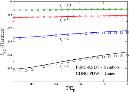
Figure 1: (Color online) Finite-$T$ exchange and correlation free energy $f_{xc}(r_{s},T)$ per electron (Hartrees) versus the reduced temperature $T/E_{F}$ in units of the Fermi energy. The symbols, labeled PIMC-KSDT are the fit given by Karasiev et al., Ref. KSDT to the path-integral Monte Carlo (PIMC) data of Brown et al., Ref. Brown13 . The continuous lines, labeled CHNC-PDW are from the classical-map HNC procedure of Perrot and Dharma-wardana, Ref. pdw2000 . The temperature range $0<T/E_{F}\leq 1$ is the region of interest for WDM studies.

II Exchange-correlation at finite-$T$

It may be useful to present this section as an ‘FAQ’ (frequently asked questions) rather than a formal discussion on thermal-XC functionals.

II.1 Do we have reliable thermal-XC functionals?

The finite-$T$ XC-functional in the random-phase approximation (RPA) RajGupt ; PDW84 ; Callaway has been available since 1982, while formulations and parametrizations that go beyond RPA have been available since the late 1980s Dandrea ; Ichimaru ; pdw2000 . Finite-$T$ XC-data from quantum simulations for the uniform finite-$T$ electron fluid were provided in 2013 by Brown et al. Brown13 , while an analytical fit to their data is found in Karasiev et al. KSDT . The XC-parametrization of Perrot and Dharma-wardana given in 2000, Ref. pdw2000 , was based on a coupling-constant evaluation of the finite-$T$ electron-fluid PDF calculated via the Classical-map Hyper-Netted-Chain (CHNC) prl1 method. It closely agrees with the recent quantum-simulation results (Fig 1). Finite-$T$ CHNC-based results are available for the 2D- and 3D- electron gas, as well as other electron-layer systems prl3 ; 2v2d ; thick2d . They are in good agreement with path-integral and other Monte Carlo (PIMC) calculations where available.

We consider the data for the 3D system that have been conveniently parametrized by Karasiev et al., (labeled KSDT in Fig. 1). The CHNC $f_{xc}(T)$ at high temperatures (beyond what is displayed in the figure) show somewhat less correlation than given by PIMC, but correctly approaches the Debye-Hückel limit at high temperatures. In the high-density regime ($r_{s}<1$), the RPA-functionals become increasingly accurate as $r_{s}\to 0$. The small-$r_{s}$ regime has also been recently treated by Schoof et al. Schoof . It should be stated that when the CHNC mapping was constructed, Frano̧is Perrot and the present author did not attempt to map the $r_{s}<1$ regime in detail as it is fairly well treated by RPA methods. Recent simulations by Malone et al. Malone find some differences between their work, and that of Brown at al for $r_{s}$ in the neighbourhood of unity. Similarly, the CHNC data show differences for the $r_{s}=1$ curve, as shown in Fig 1. However it is too early to re-examine the small $r_{s}$ regime and review the data of Ref. Malone which are given as the internal energy and not converted to a free energy.

However, it is clear that there is no shortage of reliable finite-$T$ XC-functionals for those who wish to use them.

II.2 Can we ignore thermal corrections and use the $T=0$ implementations?

While finite-$T$ XC functionals can be easily incorporated into the NPA model or average-atom cell models etc. Lieberman , this is much more difficult in the context of large DFT codes like VASP or ABINIT. Hence the already installed $T=0$ XC-functionals have been used as a part of the ‘package’ for a significant number of calculations for WDM materials, ranging from equation of state (EOS), X-ray Thomson scattering, conductivity etc. Hence the question has been raised as to whether the thermal corrections to the $T=0$ XC-functional may be conveniently disregarded.

The push for accurate XC-functionals in quantum chemistry came from the need for ‘chemical accuracy’ in predicting molecular interactions in the milli-Rydberg range. The current level of accuracy in WDM experiments is nowhere near that. Furthermore, many properties (e.g., the EOS and the total energy) are insensitive to details since total energies are usually very large compared to XC-energies, even at $T=0$, unless one is dealing with unusually contrived few-particle systems. However, one can give a number of counter examples which are designed to show that there are many situations where the thermal modification of the $T=0$ XC-energy and XC-potential are important.

As a model system we may consider the uniform electron fluid with a density of $n$ electrons per atomic volume, and thus having an electron-sphere radius $r_{s}=\{3/(4\pi n)\}^{1/3}$. Since the Fermi momentum $k_{F}=1/(\alpha r_{s})$, where $\alpha=(4/9\pi)^{1/3}$, the kinetic energy at $T=0$ scales as $1/r_{s}^{2}$, while the Coulomb energy scales as $1/r_{s}$. Hence the ratio of the Coulomb-interaction energy to the kinetic energy scales as $r_{s}$. Thus, the electron-sphere radius $r_{s}$ is also the ‘coupling constant’ that indicates the deviation of the system from the non-interacting independent particle model. The RPA is valid when $r_{s}<1$ for $T=0$ systems, for Coulomb fluids. On the other hand, at very high temperatures, the kinetic energy becomes $T$ (or $k_{B}T$ where $k_{B}=1$ in our units), while the Coulomb energy is $Z^{2}/r_{s}$, where $Z=e=-1$ for the electron fluid. Hence the ratio of the Coulomb energy to the kinetic energy, viz., $\Gamma=Z^{2}/(r_{s}T)$ for Classical Coulomb systems. Here the role of $r_{s}$ is reversed to that at $T=0$, and the system behaves as an “ideal gas” for large $r_{s}$ in systems where $T\gg E_{F}$. The equivalent of the RPA-theory in the high-$T$ limit is the Debye-Hückel theory which is valid for $\Gamma<1$. A generalized coupling constant that ‘switches over’ correctly from its $T=0$ behavior to the classical-fluid behaviour at high $T$ can be given as:

$$\Gamma(r_{s},T) = P.E/K.E=Z^{2}/(r_{s}T_{kin})$$ (1)

$$\Gamma(r_{s},T\to 0) = r_{s},\;\;\Gamma(r_{s},T\to\infty)=Z^{2}/(r_{s}T)$$ (2)

The equivalent kinetic temperature $T_{kin}$ referred to in the above equation can be constructed from the mean kinetic energy as in Eq. (A2) given in the appendix to Ref. pdw2000 . However, the main point here is that there are two non-interacting limits for studying Coulomb fluids. We can start from the $T=0$ non-interacting limit and carry out perturbation theory, or coupling-constant integrations to include the effect of the Coulomb interaction $\lambda Z^{2}/r$, with $\lambda$ moving from 0 to unity (e.g., see Eq. 71 of Ref. ppgb13 for a discussion and references). Alternatively, we can start from the $T\to\infty$ non-interacting limit. This high temperature limit is the ‘classical limit’ where the system is a non-interacting Boltzmann gas. One can do perturbation theory as well as coupling constant integrations over $\Gamma^{\prime}$ going from 0 to its required value $\Gamma$. The latter approach is well known in the theory of classical fluids. Such results provide standard ‘benchmarks’ in the context of the classical one-component plasma BausHan80 ; Ichimaru , just as the electron gas does for the quantum many-electron problem. However, there is no clear way of evolving from a classical Boltzmann gas at $\Gamma=0$ into a quantum fluid by increasing the Coulomb coupling to its full value, as the anti-symmetry of the underlying wavefunction needs to be included. This problem does not arise if we start from a non-interacting Fermi gas at $T=0$. How this problem is solved within a classical scheme is discussed below, in the context of the CHNC method. The ‘temperature connection formula’ referred to recently by Burke et al. BurkeSPB in a thermal-DFT context may be closely related to this discussion.

Although XC effects are important, it is a small fraction of the total energy. They become negligible as $T$ becomes very large, when the total energy itself becomes very large. Thus it is easy to understand that finite-$T$ XC effects are most important, for any given $r_{s}$, in the WDM range where $0\leq T/E_{F}\leq 1$, with $E_{F}=0.5/(\alpha r_{s})^{2}$. Furthermore, in any electron-ion system containing even one bound state, the electron density $n(r)$ becomes large as one approaches the atomic core, and hence there are spatial regions $r$ where $T/E_{F}(r)\leq 1$, when finite-$T$ XC comes into play. Since the ‘free-electron’ states are orthogonal to the core states, the free-electron density pile-up $n_{f}(r)$ near a nucleus immersed in a hot-electron fluid is also equally affected, directly and via the core. Furthermore, $n_{f}(r)$ is a property that directly enters into the calculation of the X-Ray Thomson scattering signal as well as the electron-ion pseudopotential $U_{ei}(r)$. Hence the effect of finite-$T$ XC, and the need to include thermal-XC functionals in such calculations can be experimentally ascertained.

In Fig. 2 we present the $n_{f}(r)$ near an Aluminum nucleus in an electron fluid of density $1.81\times 10^{23}$ electrons/cm³, i.e., at $r_{s}=2.07$ and at $T=10$ eV, calculated using the neutral-pseudo-atom method. This temperature corresponds to $T/E_{F}\simeq 0.84$. Calculations using VASP code for an actual experiment covering this regime has also been given by Plageman et al. Pleg15 . Although the difference in charge densities that arises from the difference between the $T=0$ XC and the finite-$T$ XC shown in Fig. 2 may seem small, such charge-density differences translate into significant energy differences as well as into significant X-ray scattering features.

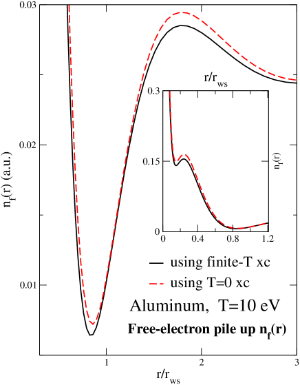
Figure 2: (Color online) The NPA free-electron density $n_{f}(r)$ using PDW finite-$T$ XC and with the $T=0$ XC. Inset: $n_{f}(r)$ inside the Wigner-Seitz sphere, with $r_{ws}\simeq$ 3.0 Bohr.

Although Kohn-Sham energies are not to be interpreted as the one-particle excitation energies of the system, they can be regarded as the one-particle energies of the non-interacting electron fluid (at the interacting density) that appears in Kohn-Sham theory. These eigen-energies are also sensitive to whether we use the $T=0$ XC-functional, or even to different finite-$T$ functionals. For instance, in Sec. 6 of Ref. pdw2000 we give the Kohn-Sham energy spectrum of warm-dense Aluminum at 15 eV calculated using the PDW-finite-$T$ XC-functional pdw2000 , as well as the finite-$T$ Iyatomi-Ichimaru (YI) functional. In summary, the KS-bound states obtained by the two methods (with YI given second) are: at energies (in Rydbergs) of 2115.044 and 2110.199 for the 1s level, 27.86214 and 27.53968 for the 2s level. The outermost level, the 2p-state, has an energy of 25.05646 and 24.81116 from PWD and YI, respectively. Similar proportionate changes are seen in the phase shifts of the continuum states. Thus it is clear that the XC-potentials should have a significant impact, especially in determining the regimes of plasma phase transitions pdw-Al ; Norman68 , finite-$T$ magnetic transitions, as well as in the theory of ionization processes Vinko15 and transport properties.

Another example of the need for finite-$T$ XC functionals is given by Sjostrom and Daligault SjostromDalig14 in their discussion of gradient-corrected thermal functionals. They conclude that “finite- temperature functionals show improvement over zero-temperature functionals, as compared to path-integral Monte Carlo calculations for deuterium equations of state, and perform without computational cost increase compared to zero-temperature functionals and so should be used for finite-temperature calculations”.

Karasiev et al. KaraQE have recently implemented the PDW-finite-$T$ XC functional as well as their new fit to the PIMC data in the ‘Quantum Espresso’ code. They have made calculations of the bandstructure and electrical conductivity of WDM Aluminum. They find that the use of finite-$T$ XC is necessary if significant errors (upto 15% at $T/Ef\simeq$ 0.11 in the case of Al) are to be avoided KaraWDM .

II.3 Can we define free and bound electrons in an ‘unambiguous’ manner?

In a ‘fully-ionized’ plasma all the electrons are in delocalized states. Thus, in stark contrast to quantum chemistry, most of plasma physics deals with continuum processes. WDM systems usually contain some partially occupied bound states as well as continuum states. Thus, if the Hamiltonian is bounded, and if there is no frequency dependent external field acting on the system, there is no difficulty in identifying the bound states and continuum states of the non-interacting electron system used in Kohn-Sham theory. If a strong frequency-dependent external field is acting on the system, the concept of ‘bound’ electrons as distinct from ‘free’ electrons becomes much more hazy, and will not be discussed here.

Depending on the nature of the ‘external potential’, a system at $T=0$ may be such that all electrons are in ‘bound states’. The latter are usually eigenstates $\psi_{j}$ whose square $\psi_{j}(r)$ become rapidly negligible as $r$ goes beyond a region of localization. The spectrum contains occupied and unoccupied ‘bound states’ as well as positive-energy states which are not localized within a given region. All states become partially occupied in finite-$T$ systems, and treatments that restrict themselves to a small basis set of functions localized over a finite region of space become too restrictive. Most DFT codes use a simulation cell of linear dimension $L$ with periodic boundary conditions. In such a model the smallest value of $k$ in momentum space is $\sim\pi/L$ and this prevents the direct evaluation of various properties (e.g., $S(k)$) as $k\to 0$. In the NPA model a large sphere of radius $R$ such that all particle correlations have died out is used, and phase shifts of continuum states, taken as plane waves, are calculated. This procedure allows an essentially direct access to $k\to 0$ properties as well as the bound and continuum spectrum of the ion in the plasma. However, the difficulty arises when the electronic bound-states spread beyond the Wigner-Seitz radius of the ion.

The question of determining the number of free electrons per ion, viz., $\bar{Z}$ is usually posed in the context of the mean-ionic charge $\bar{Z}$ used in metal physics and plasma theory. If the nuclear charge is $Z_{n}$, and if the total number of bound electrons attributed to that nucleus is $n_{b}$, then clearly $\bar{Z}=Z_{n}-n_{b}$ if the charge distribution $n_{b}(r)$ is fully contained within the Wigner-Seitz sphere of the ion. While $n_{b}$ is well-defined in that sense for many elements under standard conditions, giving, for example $\bar{Z}=3$ for Al at normal compression and up to about $T$=20 eV, this simple picture breaks down for many elements even under normal conditions. If the electronic charge density cannot be accurately represented as a superposition of individual atomic charge densities, the definition of $n_{b}$ becomes more complicated since a bound electron may be shared between two or more neighbouring atoms that form bonds. Transition-metal solids and WDMs have $d$-electron states which extend outside the atomic Wigner-Seitz sphere. Hence assigning them to a particular nuclear center becomes a delicate exercise. However, even in such situations there are meaningful ways to define $n_{b}$ and $\bar{Z}$ that lead to consistence with experiment. In such situations the proper value of $\bar{Z}$ may differ from one physical property to another as the averaging involved in constructing the mean value $\bar{Z}$ may change. A similar situation applies to the effective electron mass $m^{*}_{e}$ which deviates from the ideal value of unity (in atomic units), and takes on different values according to whether we are discussing a thermal mass, an optical effective mass, or a band mass that we may use in a Luttinger-Kohn $k\cdot p$ calculation.

Experimentally, $\bar{Z}$ is a measure of the number of free electrons released per atom. This can be measured from the $\omega\to 0$ limit of the optical conductivity $\sigma(\omega)$. Thus, although transition metals like gold have delocalized $d$-electrons, the static conductivity upto about 2 eV is found to indicate that $\bar{Z}=1$, with the optical mass $m^{*}_{e}=1$. Another property which measures $\bar{Z}$ is the electronic specific heat. Here again the specific heat evaluated from DFT calculations that use a $\bar{Z}=1$ pseudopotential for Au agrees with experimental data up to 2 eV, while those that use the density of states from all 11 electrons as free-electron states will obtain significantly different answers Vermont ; chen2013 that need to be used with circumspection. That is, such a calculation will be valid only if the $d$-electrons are fully delocalized and partake in the heating process by being coupled with the pump laser creating the WDM.

The argument that $\bar{Z}$ is not a valid concept or a quantum property because there is no ‘operator’ corresponding to it has no merit. The temperature also does not correspond to the mean value of a quantum operator. In fact, $T$ is a Lagrange multiplier ensuring the constancy of the Hamiltonian within the relevant times scales, while $\bar{Z}$ is the Lagrange multiplier that sets the charge neutrality condition $\bar{n}=\bar{Z}\bar{\rho}$ relating the average electron density to the average ion density dwp82 .

Additional discussions regarding $\bar{Z}$ may be found in Refs. cdw-CPP ; ppots12 and in Ref. pdw-Al where the case of a WDM mixture of ions with different ionization, viz., Al${}^{Z_{j}+}$ is treated within a first-principles DFT scheme.

III Future challenges in formulating finite-$T$ XC functionals

In considering a system of ions with a distribution $\rho(\vec{r})=\sum_{j}\delta(\vec{r}-\vec{R}_{j})$, and an electron distribution interacting with it, the free energy $F$ has to be regarded as a functional of both $\rho(r)$ and $n(r)$. Hence the ground state has to be determined by a coupled variational problem involving a constrained-search minimization with respect to all physically possible electron charge distributions $n(r)$, and ion distributions $\rho(r)$, subject to the usual formal constraints of $n$-representability etc. The Euler-Lagrange variational equation from the derivative of $F$ with respect to $n(r)$, for a fixed $\rho(r)$ would yield the usual Kohn-Sham procedure with the rigid electrostatic potential of $\rho(r)$ providing the external potential. However, if no static approximation or Born-Oppenheimer approximation is made, we can obtain another Euler-Lagrange variational equation from the derivative of $F$ with respect to $\rho$. This coupled pair of equations treated via density-functional theory involves not only the $f_{xc}^{ee}$, but also $f_{xc}^{ei}$ and $f_{c}^{ii}$, the latter involving correlations (but no exchange) as it arises from ion-ion interactions beyond the self-consistent-field approximation. In effect, just as the electron many-body problem can be reduced to an effective one-body problem in the Kohn-Sham sense, we can thus reduced the many-ion problem into a “single-ion problem”. Such an analysis was given by us long ago dwp82 .

The ion-ion correlations cannot be approximated by any type of local-density approximation, or even with a sophisticated gradient approximation. However, Perrot and the present author were able to show that a fully non-local approximation where an ion-ion pair-distribution can be constructed in situ using the HNC equation provides a very satisfactory solution. This is equivalent to positing that the ion-ion correlation functional is made up of the hyper-netted-chain diagrams. However, significant insights are needed in regard to the electron-ion correlation functionals which involve the coupling between a quantum subsystem and a classical subsystem. This is largely an open problem that we have attempted to deal with via the classical-map HNC approach, to be discussed below.

The advent of WDM and ultra-fast matter has thrown out a number of new challenges to the implementation of thermal DFT. A simple but at the moment unsolved problem in UFM may be briefly described as follows. A metallic solid like Al at room temperature ($T_{r}$) is subject to a short-pulse laser which heats the conduction electrons to a temperature $T_{e}$ which may be 6 eV. The core electrons (which occupy energy bands deep down in energy and hence not excitable by the laser) remain essentially unperturbed in the core region and at the core temperature, i.e., at $T_{r}\simeq$ 0.026 eV. The temperature relaxation by electron-ion processes is ‘slow’, i.e., it occurs in pico-second times scales. On the other hand, electron-electron processes are ‘fast’, and hence one would expect that the conduction-band electrons at $T_{e}$ to undergo exchange as well as Coulomb scattering within femto-second time scales, consistent with electron-electron interactions timescales. Thus, while we have a quasi-equilibrium of a two-temperature system holding for up to pico-second timescales, the question arises if one can meaningfully calculate an exchange and correlation potential between the bound electrons in the core at the temperature $T_{r}$, and the conduction-band electrons at $T_{e}$, with $T_{e}\gg T_{i}$. While we believe on physical grounds that a thermal DFT is applicable at least in an approximate sense, an unambiguous method for calculating the two-temperature XC-energies and potentials is as yet unavailable.

III.1 Classical-map Hyper-Netted Chain Method

Once the pair-distribution function of a classical or quantum Coulomb system is known, all the thermodynamic functions of the system can be calculated from $g(r)$. The XC-information is also in the $g(r)$. Only the ground-state correlations are needed in calculating the linear transport properties of the system. Hence, most properties of the system become available. It is well known that correlations among classical charges (i.e, ions) can be treated with good accuracy via the the hyper-netted-chain equation, but dealing with the quantum equivalent of hyper-netted-chain diagrams for quantum systems is difficult, even at $T=0$  FermiHNC .

When we have an electron subsystem interacting with the ion subsystem, obtaining the PDFs becomes a difficult quantum problem even via more standard methods. We need to solve for a many-particle wavefunction which rapidly becomes intractable as the number of electrons is increased beyond a small number. The message of DFT is that the many-body wavefunction is not needed, and that the one-particle charge distribution $n(r)$ is sufficient. While the charge distribution at $T=0$ involves a sum over the squares of the occupied Kohn-Sham wavefunctions, at very high $T$ the classical charge distribution is given by a Boltzmann distribution containing an effective potential felt by a single ‘field’ particle, and characterized by the temperature which is directly proportional to the classical kinetic energy.

In CHNC we attempt to replace the quantum-electron problem by a classical Coulomb problem where we can use a simple method like the ordinary HNC equation to directly obtain the needed PDFs, at some effective ‘classical fluid’ temperature $T_{cf}$ having the same density distribution as the quantum fluid. The electron PDF $g^{0}(r)$ of the non-interacting quantum electron fluid is known at any temperature and embodies the effect of quantum statistics (Pauli principle). Hence we can ask for the effective potential $\beta V_{Pau}(r)$ which, when used in the HNC, gives us the $g^{0}(r)$, an idea dating back to a publication by F. Lado Lado . This ensures that the non-interacting density has the required “$n$-representable” form of a Slater determinant. Of course, only the product $P(r)=\beta V_{Pau}(r)$ can be determined by this method, and it exists even at $T=0$. Then the total pair potential to be used in the equivalent classical fluid is taken as $\beta\phi(r)=P(r)+\beta V_{Cou}(r)$. How does one choose $\beta=1/T_{cf}$ since the Pauli term is independent of it?

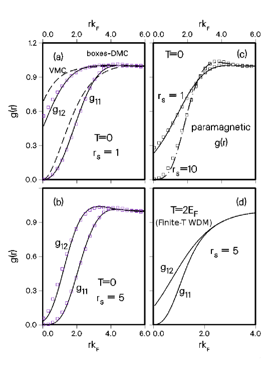
Figure 3: (a) Here the CHNC g(r) are compared with VMC and DMC simulation results: the interacting PDFs $g_{11}(r)$ and $g_{12}(r)$ at $r_{s}$=1 are shown. Solid lines:-CHNC, boxes:-DMC, dashed line:-VMC vms-dms . Panel (b) $r_{s}=5$, DMC vms-dms and HNC. In (c) the paramagnetic $g(r)$ at $r_{s}$=1 and $r_{s}$=10, T=0 are compared with DMC. (d)Finite temperature PDFs (CHNC) for $T/E_{F}$=2, $r_{s}$=5 would correspond to a WDM at $\simeq$ 3.6 eV ($\sim$ 42,000 K).

To a very good approximation, if $T_{cf}$ is chosen such that the classical fluid has the same Coulomb correlation energy $E_{c}$ as the quantum electron fluid, then it is found that the PDF of the classical Coulomb fluid is a very close approximation to the PDF of the quantum electron fluid at $T=0$. There is of course no mathematical proof of this. However, from DFT we know that only the ‘correct’ ground state distribution will give us the correct energy, and perhaps it is not surprising that this choice is found to work. The $T_{cf}$ that works for the $T=0$ quantum electron gas is called the “quantum temperature” $T_{q}$. More details of the method are given in Ref. pdw2000 . There it is argued that, to a good approximation, for a finite-$T$ electron gas at the physical temperature $T$, the effective classical fluid temperature $T_{cf}=\sqrt{T_{q}^{2}+T^{2}}$. This has been confirmed independently by Datta and Dufty SPanDufty in their study of classical approximations to the quantum electron fluid. Thus CHNC provides all the tools necessary for implementing a classical HNC calculation of the PDFs of the quantum electron gas at finite-$T$.

We display in Fig. 3 pair-distribution functions calculated using CHNC, and those available in the literature from quantum simulations at $T=0$, as finite-$T$ PDFs from quantum simulations are hard to find. In any case the classical map is expected to be better as $T$ increases and the $T=0$ comparison is important. In the figure, diffusion Monte Carlo (DMC) and variational Monte Carlo (VMC) datavms-dms are compared with CHNC results. In fig. 3 the parallel-spin PDF is marked $g_{11}(r)$, while the anti-parallel spin PDF is marked $g_{12}(r)$. The latter has a finite value as $r\to 0$ as there is no Pauli exclusion principle operating on them. Furthermore, the the mean value of the operator of the Coulomb potential, i.e., $e^{2}/r$, is of the form $\{1-\exp(-k_{dB}r)\}/r$, where $k_{dB}$ is the thermal de Broglie wavelength of the electron pair, as discussed in Ref. prl1 . This ‘quantum-diffraction’ correction ensures that $g_{12}(r\to 0)$ has a finite value, as seen in the figure. It is in good agreement with Quantum Monte Carlo results. Thus the CHNC is capable of providing a good interpretation of the physics underlying the results of quantum simulations. Needless to say, unlike Quantum Monte Carlo or Path-Integral simulation methods, the CHNC integral equations can be implemented on a laptop and the computational times are imperceptible.

Using the PDFs $g(r,T,\lambda)$ calculated with a scaled Coulomb potential $\lambda V_{Cou}(r)$, a coupling constant integration over $\lambda$ can be carried out to obtain the XC-free energy $F_{xc}(r_{s},T)$ as described in detail in Ref. pdw2000 . As seen from Fig. 1, this procedure leads to good agreement with the thermal-XC results from the PIMC method, while only the $T=0$ spin-polarized $E_{c}$ data were used in constructing $T_{q}$. Furthermore, since $T_{cf}$ tends to the physical temperature at high $T$, and since the HNC provides an excellent approximation to the PDFs of the high-$T$ electron system, the method naturally recovers the high-$T$ limit of the classical one-component plasma. Note that we could NOT have started from the high-$T$ limit of an ideal classical gas and used the well-known classical coupling constant (i.e., $\Gamma$ integration method, e.g., see Baus and Hansen or Ichimaru BausHan80 ; Ichimaru ) to determine $f_{xc}$ from an integration that ranges from $\Gamma=0,T=\infty$ to the needed temperature (i.e, the needed $\Gamma$). This is because there is no clear method of capturing the physics contained in $T_{q}$, and ensuring that Fermi statistics are obeyed (e.g., via the introduction of a $\beta V_{Pau}(r)$), as there is only Boltzmann statistics at $\Gamma=0$.

The ability of the CHNC to correctly capture the thermal-DFT properties of the finite-$T$ quantum fluid suggests its use for electron-ion systems like compressed hydrogen (electron-proton gas), or complex plasmas with many different classical ions interacting with electrons hug , without having to solve the Kohn-Sham equations as in Bredow et al. Bredow15 . The extensive calculations of Bredow et al. establish the ease and rapidity provided by CHNC, without sacrificing accuracy. CHNC has potential applications for electron-positron systems or electron-hole systems where both quantum components can be treated via the classical map. It also provides a partial solution to the still unresolved problem of formulating a fully-nonlocal ‘orbital-free’ approach that directly exploits the Hohenberg-Kohn-Mermin theory, without the need to go via the Kohn-Sham orbital formulation.

IV Conclusion

We have argued that our current knowledge of the thermal XC-functionals is satisfactory and the stage is set for their implementation in practical DFT codes. Noting the complexity of warm-dense matter, we have emphasized simplifications as well as extensions which do not sacrifice accuracy. In this respect the neutral-pseudo atom model can, in most cases do the work of the ab initio codes like VASP, and handle high-temperature problems that are beyond their scope. Orbital-free approaches KaraQE will also become increasingly useful, especially at intermediate and high $T/E_{F}$. Nevertheless, the ab initio codes are needed at low-temperature low-density situations involving molecular formation, where the NPA breaks down as it is a “single-center” approach. However, in many WDM cases, we need to go beyond the picture where the ion subsystem is held static, and the electrons only feel them as an ‘external potential’. Hence we have emphasized the need for calculating not just the XC-functionals for electrons, but also the classical correlation functionals for ions, as well as the ion-electron correlations directly, in situ, via direct coupling-constant integrations of all the pair-distribution functions of the system, ensuring a fully non-local formulation where gradient expansions are not needed. In fact, there is no need for any XC-functionals in such a scheme. To do this efficiently and accurately, we have proposed a classical map of the quantum electrons and implemented it in the CHNC scheme which depends on DFT ideas. This capacity is not found in any of the currently available methods. CHNC has been used to construct a finite-$T$ XC functional for electrons more than a decade before PIMC results became available, and it turns out that the CHNC results are accurate. The CHNC scheme has been successfully used for calculating the equation of state and other properties of warm dense matter as well as multi-component $T=0$ electron-layer systems, thick layers etc., that are expensive to treat by quantum simulation methods, but relevant for nanostructure physics.

References

- (1) J. M. Luttinger and J. C. Ward, Phys. Rev. 1960 118, 1417; W. Kohn and J. M. Luttinger, Phys. Rev., 1960, 118 41
- (2) Takahashi, Y.; and Umezawa, H.; Thermofield Dynamics. In, Collective Phenomena, Vol 2, Gordon and Beach, New York USA 1975 pp 55-80; Reprinted in: Int. J. Mod. Phys. B 1996 10, 1755
- (3) Heslot, A.; Phys. Rev. D 1985 31 1341
- (4) Hohenberg P. and Kohn W.; Phys. Rev. 1964 136, B864; Kohn W. and Sham, L. J.; Phys. Rev. 1965 140, A1133
- (5) Mermin, N. D.; Phys. Rev. 1965 137 A1441.
- (6) Dharma-wardana M. W. C.; A Physicists’s View of Matter and and Mind 2014 World Scientific, Singapore;
- (7) Dharma-wardana M. W. C.; J. Phys. Conf. Ser. 2013 442, 012030; doi:10.1088/1742-6596/442/1/012030
- (8) Graziani, F., Desjarlais M. P., Redmer, R. and Trickey, S. B. Eds., Frontiers and Challenges in Warm Dense Matter, Lecture Notes in Computational Science and Engineering, 2014 96 Springer International Publishing, Germany.
- (9) Milchberg, H. M., Freeman, R. R., Davy, S. C., and More, R. M.; Phys. Rev. Lett. 1988 61, 2364;
- (10) Ng, Andrew; Int. J. Quant. Chem. 2012 112, 150.
- (11) Dharma-wardana M. W. C.; Phys. Rev. E 2001 64, 035432(R); Benedict, Lorin X.; Surh, M. P.; Castor, John; Khairallah, S. A.; Whitley, H. D.; Richards, D. F.; Glosli, D. N.; Murillo, M. S.; Scullard, C. R.; Grabowski, P. E.; Michta, David; and Graziani, Frank R.; Phys. Rev. E 2012 86, 046406.
- (12) Driver, K. P.; and Militzer, B.; Phys. Rev. Lett. 2012 108, 115502
- (13) Lorazo, P.; Lewis, L. J.; and Meunier, M.; Phys. Rev. Lett. 2003 91, 225502; Phys. Rev. B 2006 73, 134108.
- (14) Shah, Jagdeep; Ultrafast Spectroscopy of Semiconductor Nanostructures, Springer (1999); Dharma-wardana M. W. C.; Solid State Com. 1993] [86, 83.
- (15) Dagens, L.; J. Phys. C 1972 5, 2333 Dagens, L.; J. Phys. (Paris) 1975 36, 521
- (16) Ziman, J. H.; Advances in Physics 1964 49 89-138
- (17) Dharma-wardana M. W. C.; Contr. Plasma Phys. 2015 55, 85-101
- (18) Gilbert, T. L., Phys. Rev. B 1975 12, 2111
- (19) Perrot, F.; Phys. Rev. B 1993 47, 570
- (20) Perrot, F.: and Dharma-wardana, M. W. C.; Phys. Rev. E. 1995, 52, 5352
- (21) Dharma-wardana, M. W. C.; and Perrot, F.; Phys. Rev. A 1982 26, 2096
- (22) Wilson, J. C. et al; J.Quant. Spec. and rad. Transfer. 2006, 99 658-679
- (23) Liberman, P. D. A.; J. of Quant. Spect. And Rad. Transfer, 1982 27, 335
- (24) Starrett, C. E.; and Saumon, D.; Phys. Rev. E 2015 92, 033101
- (25) Chihara, J.; Kambayashi, S. J Phys: Condens matter 1994, 6, 10221.
- (26) Dharma-wardana, M. W. C.; Int. J. Quant. Chem. 2012 112 53-64
- (27) Harbour, L.; Dharma-wardana, M. W. C.; Klug, D. D, and Lewis, L.; Contr. Plasma Phys. 2015 55, 144-151
- (28) Recoules, V.; Clérouin, J.; Zérah, G.; Anglade, P. M.; and Mazevet, S.; Phys. Rev. Lett. 2006 96, 055503.
- (29) Dharma-wardana, M. W. C.; Taylor, T.; J.Phys. C 1981 14 629
- (30) Gupta, U.; and Rajagopal, A. K.; Phys. Reports 1982 87 259
- (31) Perrot, F.; and Dharma-wardana, M. W. C.; Phys. Rev. A 1984 30 2619
- (32) Kanhere, D. C.; Panat, P. V.; Rajagopal, A. K.; and Callaway, J.; Phys. Rev. A 1986 33, 4907
- (33) Dandrea, R. G.; Ashcroft, N. W.; and Carlsson, A. E.; Phys. Rev. B 1987 34 2097
- (34) Ichimaru, S.; Iyetomi, H.; Tanaka, S.; Phys. Reports 1987 149 91
- (35) Perrot, F.; Dharma-wardana, M. W. C.; Phys. Rev. B 2000 62 16536, Erratum 2003 67, 79901
- (36) http://www.castep.org/CASTEP/CASTEP
- (37) https://www.vasp.at/
- (38) http://www.abinit.org/
- (39) https://www.scm.com/
- (40) http://www.gaussian.com/
- (41) Perdew, J. S.; Burke, K.; and Ernzerhof, M.; Phys. Rev. Lett. 1966, 77, 3865
- (42) Gonze, X.; Phys. Rev. B 1997 55, 10337
- (43) Karasiev, Valentin V.; Sjostrom, Travis,; Trickey, S. B.; Computer Physics Communications 2014 185 3240-3249.
- (44) Silvestrelli, P. L.; Alavi, A.; and Parrinello, M.; Phys. Rev. B 1997 55, 15515
- (45) Plagemann, K.U.; Rüter H.R.; Bornath T.; Shihab M.; Desjarlais M.P.; Fortmann C.; Glenzer S.H.; Redmer R.; Phys. Rev. E 2015 92 013103
- (46) P. Sperling et al., Phys. Rev. Lett. 2015 115, 115001
- (47) Vinko S. M. et al.; Investigation of femtosecond collisional ionization rates in a solid-density aluminium plasma Nature Communications 2015 6 6397
- (48) Dharma-wardana, M. W. C.; The dynamic conductivity and the plasmon profile of Aluminum in the ultra-fast-matter regime; an analysis of recent X-ray scattering data from the LCLS arXive: 1601.07566 2015
- (49) Pribram-Jones,A.; Pittalis, S.; Gross, E. K. U.; and Burke, K.; Frontiers and Challenges in Warm Dense Matter, Lecture Notes in Computational Science and Engineering, 2014 96 Springer International Publishing, Germany; arXive: 1309.3043v1
- (50) Dharma-wardana, M. W. C.; and Perrot, F.; Phys. Rev. B 2002 66, 014110
- (51) Dharma-wardana, M. W. C.; Electron-ion and ion-ion potentials for modeling warm dense matter: Applications to laser-heated or shock-compressed Al and Si. Phys. Rev. E 2012 86, 036407
- (52) Ethan W. Brown, Jonathan L. DuBois, Markus Holzman, David M. Ceperley, Phys. Rev. B 2013 88, 081102(R)
- (53) Malone, F. D. et al; http://arxiv.org/pdf/1602.05104v2.pdf.
- (54) Norman, G. E.; and Starostin, A. N.; High Temp. 1968 6, 394.
- (55) Schoof, J. T.; et al; Phys. Rev. Lett. 2015 115, 130402
- (56) Karasiev, V. V.; Sjostrom, T.; Dufty, J.; and Trickey, S. B.; Phys. Rev. Lett. 2014 112 076403
- (57) Sjostrom, Travis; and Daligault, Jéôme; Physical Review B 2014 90 155109
- (58) Karasiev, Valantin V.; Calderin, Lázaro; S.B. Trickey, S. B.; http://arxiv.org/abs/1601.04543 2015
- (59) Dharma-wardana, M. W. C.; and Perrot, F.; A simple classical mapping of the spin-polarized quantum electron gas distribution functions and local field corrections. Phys. Rev. Lett. 2000 84, 959
- (60) Perrot, François; and Dharma-wardana, M. W. C.; 2D-Electron Gas at Arbitrary Spin Polarizations and Coupling Strengths: Exchange-Correlation Energies, Distribution Functions, and the Spin-Polarized Phase. Phys. Rev. Lett. 2001 87, 206404
- (61) Dharma-wardana, M. W. C.; and Perrot, F.; Spin-polarized stable phases of the 2DES at finite temperatures. Phys. Rev. Lett. 2003 90, 136601
- (62) Dharma-wardana, M. W. C.; and Perrot, F.; Spin- and valley-dependent analysis of the two-dimensional low-density electron system in Si MOSFETs. Phys. Rev. B 2004 70, 035308
- (63) Dharma-wardana, M. W. C.; Spin and temperature dependent study of exchange and correlation in thick two-dimensional electron layers. Phys. Rev. B 2005 72, 125339
- (64) Smith, J. C.; Pribram-Jones, A.; and Burke, K. arXive:1509.03097v1 [cond-mat.str-el] 2015
- (65) Baus, M.; and Hansen, J.-P.; Physics Reports 1980 59 2; Ichimaru., S.; Rev. Mod. Phys. 1982 54 1017
- (66) Lin, Z.; Zhigilei, L. V.; and Celli, V.; Phys. Rev. B 2008 77, 075133
- (67) Chen, Z.: Holst, B.; Kirkwood, S. E.; Sametoglu, V.; Reid, M.; Tsui, Y. Y.; Recoules, V.; and Ng, A.; Phys. Rev. Lett. 2013 110, 135001
- (68) Zabolitsky, J. G.; Advances in Nuclear Physics Negale, W.; and Vogt, Erich.; Eds., Plenum, New York, USA 1981; pp 1-58
- (69) Lado, F.; J. Chem. Phys. 1967 47, 5369.
- (70) Dufty, J.; and Dutta, Sandipan; Phys. Rev. E 2013 87, 032101
- (71) Ortiz, G.; and Ballone, P.; Phys. Rev. B 1994 50, 1391
- (72) Bredow1, R.; Bornath, Th.; Kraeft, W.-D.; Dharma-wardana, C.; and Redmer, R. Contributions to Plasma Physics 2015 55 222-229