Disruption of Planetary Orbits Through Evection Resonance with an External Companion: Circumbinary Planets and Multiplanet Systems

Abstract

Planets around binary stars and those in multiplanet systems may experience resonant eccentricity excitation and disruption due to perturbations from a distant stellar companion. This “evection resonance” occurs when the apsidal precession frequency of the planet, driven by the quadrupole associated with the inner binary or the other planets, matches the orbital frequency of the external companion. We develop an analytic theory to study the effects of evection resonance on circumbinary planets and multiplanet systems. We derive the general conditions for effective eccentricity excitation or resonance capture of the planet as the system undergoes long-term evolution. Applying to circumbinary planets, we show that inward planet migration may lead to eccentricty growth due to evection resonance with an external perturber, and planets around shrinking binaries may not survive the resonant eccentricity growth. On the other hand, significant eccentricity excitation in multiplanet systems occurs in limited parameter space of planet and binary semimajor axes, and requires the planetary migration to be sufficiently slow.

1 Introduction

Evection resonance is a secular-orbital resonance between the apsidal precession of a planet or satellite due to the quadrupole moment of a central body and the orbital motion of a distant perturber. This resonance was first studied in the context of the Moon-Earth-Sun system by Touma & Wisdom (1998), who showed that the resonance between the Moon’s orbital precession due to the Earth’s oblateness and the periodic perturbation of the Sun could give the Moon a significant eccentricity in its early evolution, which later produce the misalignment of the Moon’s orbit. Recently, Spalding, Batygin & Adams (2016) studied the evolution of exomoons during planetary migration, and showed that evection resonance could induce eccentricity growth of exomoons, leading to their collisions with the host planet.

A recent study by Touma & Sridhar (2015) examined the effect of evection resonance in multiplanet systems perturbed by distant binary companions. For such a system, the evection resonance occurs between one of the precession modes of the planets, which is similar to the apsidal precession the outer planet due to the quadrupole moment from the inner massive planets, and the orbital motion of the binary. It was showed that planetary migration can trap the outer planet into an evection resonance, resulting in significant planetray eccentricity excitation and possibly disruption. Touma & Sridhar (2015) suggested that such resonant driving of eccentricity by binary may have altered the architecture of many multiplanet systems and weaken the multiplanet occurrence rate in wide binaries.

Evection resonance may also play role in circumbinary planet systems. About 10 binary star systems harboring transiting circumbinary planets have been discovered by the Kepler mission (e.g. Doyle et al. 2011; Kostov et al. 2015). However, no transiting circumbinary planet has been found around compact stellar binaries with periods $\lesssim 7$ days, despite the large number of such compact eclipsing binaries in the Kepler sample. It is generally believed that close binaries (with periods $\lesssim 5$ days) are not primordial, but have formed at a wider separation and subsequently shrunk via Lidov-Kozai (LK) cycles with tidal friction induced by an inclined tertiary companion (Fabrycky & Tremaine, 2007). Several papers have examined the dynamics of “binary + planet” systems in the presence of distant stellar companions (Muñoz & Lai 2015; Martin, Mazeh & Fabrycky 2015; Hamers, Perets & Portegies Zwart 2016). A sufficiently massive planet can suppress the shrinkage of the inner binary orbit by disrupting the LK cycles, thus explaining the lack of planet-hosting short-period binaries. Alternatively, a low-mass circumbinary planet does not affect the LK cycles of the inner binary, but becomes misaligned with the shrinking binary or becomes unstable and destructed during the binary shrinkage (Muñoz & Lai, 2015). However, in all these studies, the effect of evection resonance was not considered. As the inner binary undergoes LK oscillations and orbital decay, the apsidal precession of the planet may be resonant with the orbital motion of the tertiary companion. This can excite planetary eccentricity and may lead to the destruction of the planet.

In this paper we develop an analytic theory to study the effects of evection resonance on circumbinary planets and multiplanet systems induced by external stellar companions. In particular, we derive the general conditions for which appreciable eccentricity excitation associated with resonance passage or resonance capture can be achieved. These conditions and the expression for the maximum eccentricity can be applied to a variety of situations.

Our paper is structured as follows. In Section 2 we summarize the general theory of evection resonance for a circumbinary planet under the perturbation of a tertiary companion. We use the Hamiltonian approach, ignoring dissipative effects and long term evolution of the system (e.g., associated with planet migration or LK cycles of the inner binary). We obtain a one-parameter nondimensionalized Hamiltonian and use it to calculate the width and libration timescale of the resonance. In Section 3 we study the passage through resonance due to the long term evolution of the system by considering the evolution of the parameter of the nondimensionalized Hamiltonian. We obtain the criteria for resonant trapping, and estimate the magnitude of eccentricity excitation. In Section 4 we apply the results in Section 3 to realistic long-term evolutions of hierarchical triple systems hosting a circumbinary planet, including planet migration and the LK oscillations and orbital decay of the inner binary. In Section 5 we adapt the theory developed in Sections 2-3 to multiplanet systems with external perturbers, and examine the condition for planetary eccentricity excitation due to evection resonance. We summarize our results in Section 6.

2 Evection Resonance of a Circumbinary Planet with an External Perturber

2.1 Setup and Perturbation Potential

Consider a binary with masses $M_{1},M_{2}$ and semimajor axis $a_{b}$ orbited by a planet of mass $m_{p}$ and semimajor axis $a$ [relative to the center of mass (CM) of the binary]. The binary is in a hierarchical triple system, with an extrenal perturber of mass $M_{B}$ and semimajor axis $a_{B}$ (relative to the CM of the inner binary). We also define $M_{b}=M_{1}+M_{2}$ and $\mu_{b}=M_{1}M_{2}/M_{b}$ as the total mass and reduced mass of the inner binary, and $M_{\rm tot}=M_{b}+M_{B}$ as the total mass of the stellar triple. Throughout the paper we consider $m_{p}\ll M_{1},M_{2},M_{B}$ and $a_{b}\ll a\ll a_{B}$. For simplicity, we assume that the outer binary is circular ($e_{B}=0$), but the inner binary and the planet can have general eccentricities and inclinations. Also, in this section and Section 3 we ignore the evolution of the inner binary driven by $M_{B}$, because the timescale for this evolution is much longer than the timescale for the evolution of the planet’s orbit.

The planet experiences perturbations from both the inner and outer binaries. To the quadrupole order, the perturbing potential acting on the planet can be written as

$$\begin{split}\Phi=\Phi_{b}+\Phi_{B},\end{split}$$ (1)

where $\Phi_{b}$ is the potential from the inner binary (double-averaged over the orbits the planet and inner binary),

$$\begin{split}\Phi_{b}=&\frac{\Phi_{b0}}{8(1-e^{2})^{3/2}}\left[1-6e_{b}^{2}-3(1-e_{b}^{2})({\hat{\bf n}}_{b}\cdot{\hat{\bf n}})^{2}\right.\\ &\left.+15\,e_{b}^{2}\,({\hat{\bf e}}_{b}\cdot{\hat{\bf n}})^{2}\right],\end{split}$$ (2)

with

$$\begin{split}\Phi_{b0}=\frac{\mathcal{G}\mu_{b}a_{b}^{2}}{a^{3}},\end{split}$$ (3)

and $\Phi_{B}$ is the potential from the outer binary (averaged over the orbit of the planet),

$$\begin{split}\Phi_{B}=&\frac{\Phi_{B0}}{4}\left[-1+6e^{2}+3(1-e^{2})({\hat{\bf n}}\cdot{\hat{\bf r}}_{B})^{2}\right.\\ &\left.-15\,e^{2}({\hat{\bf e}}\cdot{\hat{\bf r}}_{B})^{2}\right],\end{split}$$ (4)

with

$$\begin{split}\Phi_{B0}=\frac{\mathcal{G}M_{B}a^{2}}{a_{B}^{3}}.\end{split}$$ (5)

In Eqs. (2) and (4), ${\hat{\bf e}}$ is the unit vector in the direction of periapsis and ${\hat{\bf n}}$ is the unit vector normal to the orbital plane of the planet, while ${\hat{\bf e}}_{b}$ and ${\hat{\bf n}}_{b}$ are the corresponding unit vectors for the inner binary; ${\hat{\bf r}}_{B}$ is the unit vector in the direction of $M_{B}$. The derivation of these potentials can be found in, e.g., Tremaine, Touma & Namouni (2009) and Tremaine & Yavetz (2014). Note that when $e_{b}\neq 0$ and $M_{1}\neq M_{2}$, the inner binary also exerts an octupole potential on the planet (e.g. Liu et al. 2015), but we ignore it here because it tends to be small for $M_{1}\sim M_{2}$. The outer binary has a zero octupole potential because it has zero eccentricity.

The ratio $\epsilon\equiv\Phi_{B0}/\Phi_{b0}$ characterizes the relative strengths of the two potentials. Throughout this paper, we consider the regime where

$$\begin{split}\epsilon\equiv\frac{\Phi_{B0}}{\Phi_{b0}}={M_{B}\over\mu_{b}}{a^{5}\over a_{b}^{2}a_{B}^{3}}\ll 1,\end{split}$$ (6)

i.e., the potential from the inner binary dominates over the outer potential. In another word, the planet lies inside the Laplace radius $a_{L}$, i.e.,

$$\begin{split}a\ll a_{L}\equiv\left({\mu_{b}\over M_{B}}\right)^{1/5}\left(a_{b}^{2}a_{B}^{3}\right)^{1/5}.\end{split}$$ (7)

To express the potential in terms of various orbital elements, we set up a Cartesian cooridnate system with the $z$-axis along ${\hat{\bf n}}_{b}$, and the $x$-axis along the direction of ${\hat{\bf n}}_{b}\times{\hat{\bf n}}_{B}$ (so the longitude of ascending node of the outer binary is $\Omega_{B}=0$). In this coordinate system, we have

$$\hat{\mathbf{n}}= \left(\begin{array}[]{l}\sin\Omega\sin I\\ -\cos\Omega\sin I\\ \cos I\end{array}\right),$$ (11)

$$\hat{\mathbf{e}}= \left(\begin{array}[]{l}\cos\Omega\cos\omega-\sin\Omega\sin\omega\cos I\\ \cos\Omega\sin\omega\cos I+\sin\Omega\cos\omega\\ \sin\omega\sin I\end{array}\right),$$ (15)

$$\hat{\mathbf{r}}_{B}= \left(\begin{array}[]{l}\cos\lambda_{B}\\ \sin\lambda_{B}\cos I_{B}\\ \sin\lambda_{B}\sin I_{B}\end{array}\right),$$ (19)

where $I$, $I_{B}$ are the inclination angles of the planetary and outer binary orbits relative to the inner binary orbit (i.e., $\cos I\equiv{\hat{\bf n}}\cdot{\hat{\bf n}}_{b}$ and $\cos I_{B}\equiv{\hat{\bf n}}\cdot{\hat{\bf n}}_{B}$), $\Omega$ and $\omega$ are the longitude of ascending node and the argument of pericenter of the planet’s orbit, and $\lambda_{B}$ is the mean longitude of the external perturber $M_{B}$. The eccentricty unit vector of the inner binary is ${\hat{\bf e}}_{b}=(\cos\varpi_{b},\sin\varpi_{b},0)$, with a constant $\varpi_{b}$ (the longitude of pericenter).

2.2 Hamiltonian Near Resonance

Since $\epsilon\ll 1$, the nodal precession of the planet induced by $\Phi_{b}$ is much faster than that induced by $\Phi_{B}$, and the planet’s orbit is strongly coupled to the inner binary. Thus, if the initial inclination angle $I$ is zero, the planet will stay aligned with the inner binary even in the presence of perturbation from the outer binary (Muñoz & Lai, 2015). In the following analysis, we assume $I=0$ at all times; this greatly simplifies the calculation without much loss of generality. In this case, the apsidal precession rate (for the longitude of pericenter $\varpi=\Omega+\omega$) of the planet induced by the inner binary is given by

$$\begin{split}\dot{\varpi}={3(2+3e_{b}^{2})\over 8(1-e^{2})^{2}}\,\frac{\Phi_{b0}}{a^{2}n}\simeq{3(2+3e_{b}^{2})\over 8}\,\frac{\Phi_{b0}}{a^{2}n},\end{split}$$ (20)

where $n=\sqrt{\mathcal{G}M_{b}/a^{3}}$ (with $M_{b}=M_{1}+M_{2}$) is the mean motion of the planet, and the second equality assumes $e\ll 1$.

Consider a planet near the “evection resonance”, where the precession rate of $\varpi$ is close to the outer binary’s orbital frequency $n_{B}=\sqrt{\mathcal{G}M_{\rm tot}/a_{B}^{3}}$ (where $M_{\rm tot}=M_{b}+M_{B}$), i.e.,

$$\dot{\varpi}\simeq n_{B}=\dot{\lambda}_{B},$$ (21)

or equivalently

$${{\dot{\varpi}}^{2}\over n_{B}^{2}}=\left[{3(2+3e_{b}^{2})\over 8}\right]^{2}\left({\mu_{b}^{2}\over M_{b}M_{\rm tot}}\right)\left({a_{b}^{4}a_{B}^{3}\over a^{7}}\right)\simeq 1.$$ (22)

Physically, the resonance occurs when the planet’s eccentricity vector librates around a fixed angle with respect to the outer binary. Avergaing out the fast-varying angles $\varpi$ and $\lambda_{B}$, we find (for $I=0$)

$$\begin{split}\Phi=&-\Phi_{b0}\left[\frac{2+3e_{b}^{2}}{8(1-e^{2})^{3/2}}+{\epsilon\over 16}\,\Bigl{[}(6+9e^{2})\cos^{2}\!I_{B}-(2+3e^{2})\Bigr{]}\right.\\ &\left.+{15\,\epsilon\over 32}\,(1+\cos I_{B})^{2}\,e^{2}\cos(2\varpi-2\lambda_{B})\right].\end{split}$$ (23)

We can nondimensionalize the Hamiltonian in the canonical coordinate and momentum (the modified Delaunay variables)

$$\begin{split}\gamma=-\varpi,\quad\Gamma=1-(1-e^{2})^{1/2}\simeq{e^{2}\over 2}.\end{split}$$ (24)

The dimensionless time is

$$\hat{t}\equiv t\,\frac{\Phi_{b0}}{na^{2}},$$ (25)

and the dimensionless Hamiltonian (for $e\ll 1$) is

$$\begin{split}\hat{H}\equiv\frac{H}{\Phi_{b0}}=(A+\epsilon B)\Gamma+C\Gamma^{2}+\epsilon D\Gamma\cos(2\gamma+2\lambda_{B}),\end{split}$$ (26)

where we have dropped a non-essential constant. The dimensionless constants $A,B,C,D$ (all of order unity) are given by

$$A= -\frac{3}{8}(2+3e_{b}^{2}),$$ (27)

$$B= \frac{3}{8}(1-3\cos^{2}\!I_{B}),$$ (28)

$$C= -\frac{3}{4}(2+3e_{b}^{2}),$$ (29)

$$D= -\frac{15}{16}(1+\cos I_{B})^{2}.$$ (30)

To further simplify the Hamiltonian, we make another canonical transformation and rescale the Hamiltonian:

$$\theta= -2\gamma-2\lambda_{B}=2\varpi-2\lambda_{B},$$ (31)

$$\Theta= \frac{C}{\epsilon D}\Gamma,$$ (32)

$$K= \frac{C}{\epsilon^{2}D^{2}}\hat{H}+\frac{n_{B}na^{2}}{\epsilon D\Phi_{b0}}\Theta,$$ (33)

$$\tau= -2\epsilon D\hat{t}=-\frac{2\epsilon D\Phi_{b0}}{na^{2}}\,t.$$ (34)

The new (dimensionless) Hamiltonian is then

$$\begin{split}K=\eta\Theta+\Theta^{2}+\Theta\cos\theta,\end{split}$$ (35)

where $\eta$ is a constant parameter given by

$$\begin{split}\eta=\frac{A+\epsilon B+(n_{B}na^{2}/\Phi_{b0})}{\epsilon D}.\end{split}$$ (36)

Using Eq. (20) we find

$$\begin{split}\eta={2(2+3e_{b}^{2})\over 5(1+\cos I_{B})^{2}}\,\,{1\over\epsilon}\left[1-{n_{B}\over\dot{\varpi}(e=0)}-\epsilon\,\left({1-3\cos^{2}\!I_{B}\over 2+3e_{b}^{2}}\right)\right].\end{split}$$ (37)

Note that the dimensionless time $\tau$ for the Hamiltonian (35) can be written as

$$\tau=2|D|\,{t\over T_{K}},$$ (38)

where

$$T_{K}^{-1}\equiv{\Phi_{B0}\over na^{2}}={M_{B}\over M_{b}}\left({a\over a_{B}}\right)^{3}n$$ (39)

characterizes the precession rate (Kozai rate) of the planet driven by the extrenal companion. The dynamical variable $\Theta$ is related to the eccentricity ($e\ll 1$) by

$$\begin{split}\Theta\simeq{C\over 2D}{e^{2}\over\epsilon}.\end{split}$$ (40)

The Hamiltonian (35) is the same as that describing the dynamics of planets near the second-order mean-motion resonance (Murray & Dermott, 1999). Thus we should expect that the resonance structure to be the same.

2.3 Structure of Resonance

Next we can examine the structure of the resonance by studying the phase space topology of the system. It is convenient to use the conjugate (Poincare) variables

$$\begin{split}X=\sqrt{2\Theta}\sin\theta,~{}~{}~{}Y=\sqrt{2\Theta}\cos\theta.\end{split}$$ (41)

The Hamiltonian becomes

$$\begin{split}K=\frac{\eta}{2}(X^{2}+Y^{2})+\frac{1}{4}(X^{2}+Y^{2})^{2}+\frac{1}{2}Y\sqrt{X^{2}+Y^{2}}.\end{split}$$ (42)

The level curves of this Hamiltonian for different $\eta$ values are shown in Fig. 1. Note that $\sqrt{X^{2}+Y^{2}}=\sqrt{2\Theta}\simeq e\sqrt{C/\epsilon D}$, the radius from the origin to the trajectory measures $e/\sqrt{\epsilon}$.

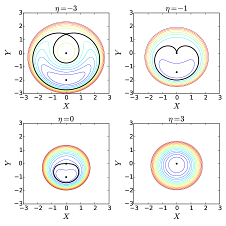
Figure 1: Level curves of the Hamiltonian for different $\eta$ values. The black dots and black lines mark the fixed points and separatrices. Two bifurcations take place at $\eta=-1$ and $\eta=1$. The bifurcation at $\eta=-1$ is shown. For $\eta<1$, there exists a libration zone; for $-1<\eta<1$, the trajectory for an initially circular orbit lies close to the separatrix and can be excited to nontrivial eccentricities.

The fixed points of the Hamiltonian follow from $\partial K/\partial X=\partial K/\partial Y=0$, and are located at $X=0$ and $Y=0$, $Y=\sqrt{-1-\eta}$ or $Y=-\sqrt{1-\eta}$. Thus, for $\eta\geq 1$, there is one stable fixed point at $(X,Y)=(0,0)$; for $\eta<1$, there are two fixed points at $(X,Y)=(0,0)$ and $(0,-\sqrt{1-\eta})$; for $\eta<-1$, there is an additional (saddle) point at $(0,\sqrt{-1-\eta})$.

We see that for $-1\leq\eta<1$, the phase-space trajectory of an initially near-circular orbit (which lies near the origin of the $XY$ space) is close to the separatrix, giving rise to nontrivial eccentricity excitation that depends weakly on the initial eccentricity. For a given $\eta\in[-1,1)$, the maximum $\Theta$ that can be achieved (corresponding to the minimum $Y$ on the separatrix) is

$$\begin{split}\Theta_{\text{max}}(\eta)=1-\eta.\end{split}$$ (43)

This gives

$$\begin{split}e_{\text{max}}(\eta)=\sqrt{\frac{2\epsilon D}{C}(1-\eta)}\qquad{\rm with}~{}\eta\in[-1,1)\end{split}$$ (44)

The “limiting eccentricity” (i.e. the maximum value of $e_{\text{max}}$ for all $\eta$) occurs at $\eta=-1$ and is given by

$$\begin{split}e_{\rm lim}=e_{\rm max}(\eta=-1)=2\sqrt{\frac{\epsilon D}{C}}.\end{split}$$ (45)

It is useful to estimate the periods of trajectories in the libration zone. These periods are generally of order unity (in terms of the dimensionless tie $\tau$), but can become larger for $\eta$ close to $\pm 1$. The equation of motion is given by

$$\frac{d\theta}{d\tau} =\frac{\partial K}{\partial\Theta}=\eta+2\Theta+\cos\theta,$$ (46)

$$\frac{d\Theta}{d\tau} =-\frac{\partial K}{\partial\theta}=\Theta\sin\theta.$$ (47)

When the trajectory has a small initial eccentricity, or $\Theta_{0}\equiv\Theta(t=0)\ll 1$, the period approximately corresponds to the time required to reach $\Theta\sim 1$. The system spends most time near the turning point of $\theta$-libration, where (for small $\Theta$) we have $\cos\theta\simeq-\eta$ and $d\ln\Theta/d\tau=\sin\theta\sim\sqrt{1-\eta^{2}}$. Thus the (dimensionless) libration period for a trajectory with small $\Theta_{0}$ is

$$\begin{split}\tau_{\rm lib}\sim\frac{|\ln\Theta_{0}|}{\sqrt{1-\eta^{2}}}.\end{split}$$ (48)

Also of interest is the trajectory doing small-amplitude oscillation around the stable fixed point $(X,Y)=(0,-\sqrt{1-\eta})$ [corresponding to $\theta=\pi$, $\Theta=(1-\eta)/2$] in the libration zone. Expanding Eqs. (46)-(47) around the fixed point (e.g. $\theta=\pi+\Delta\theta$), we find $d^{2}\Delta\theta/d\tau^{2}\simeq-(1-\eta)\Delta\theta$. The period is then

$$\begin{split}\tau_{\rm lib}\simeq\frac{2\pi}{\sqrt{1-\eta}},\end{split}$$ (49)

which is of order unity unless $\eta$ approaches $1$.

3 Resonant Passage and Capture

Having studied the dynamics of our planet-in-binaries system near the evection resonance at a constant $\eta$, we now examine the evolution of the planet’s eccentricity as the parameter $\eta$ changes slowly. Such gradual change of $\eta$ can be facilitated by the migration of the planet or the evolution of the inner binary – these specific applications will be discussed in Section 4. The slow evolution of $\eta$ can produce nontrivial excitation of the planet’s eccentricity, as the system is driven across the resonance and sometimes gets trapped in resonance. Since equation (35) has the same form as the Hamiltonian for the second-order mean motion resonance, many aspects of the resonance capture problem have been studied before (see Murray & Dermott 1999, Peale 1986 and Borderies & Goldreich 1984). These studies, however, mainly focused on the case where the orbit has a relatively large initial eccentricity (i.e. the initial $\Theta\gtrsim 1$) and the evolution of $\eta$ is infinitely slow.

In the following, we assume that the system is initially out of resonance with a small eccentricity $e_{0}$. We focus on the regime where $\epsilon$ is large enough so that $\Theta_{0}=|C/2D|(e_{0}^{2}/\epsilon)\ll 1$, which has not been covered by pervious studies. We also assume that $d\eta/d\tau$ is constant. We consider a range of values for $|d\eta/d\tau|$, from $\ll 1$ to $\sim 1$ [note that the libration rate of the resonance is of order unity; see Eqs. (48)-(49)]. The initial $\eta_{0}\equiv\eta(t=0)$ is chosen such that the system passes through resonance at some later times.

3.1 Increasing $\eta$: Eccentricity Excitation Without Trapping

Consider a system initially at $\eta_{0}<-1$ and $\Theta_{0}\ll 1$. As the parameter $\eta$ gradually increases, the system passes through the resonance and may experience significant eccentricity growth. Figure 2 depicts an example.

First consider the case when $|d\eta/d\tau|\ll 1$. Away from the sepratrix, the dynamical (libration/circulation) time of the system is $\tau_{\rm lib}\sim 1$. So when $|d\eta/d\tau|\ll 1$, the theory of adiabatic invariance implies that the phase-space area covered by the trajectory is conserved, i.e.

$${\cal A}=\oint\,Y\,dX=\oint\,\Theta\,d\theta={\rm constant}.$$ (50)

Thus, starting from $\eta_{0}<-1$ (where the system lies in the inner circulating zone), the planet maintains at its small eccentricty for $\eta<-1$. Then, near $\eta=-1$, the trajectory encounters the separatrix and experiences a jump in $\cal A$ (and eccentricity). After passing through $\eta=-1$, the separatrix continues to shrink and the system trajectory lies in the outer circulating zone, conserving its $\cal A$. Clearly, in the limit $|d\eta/d\tau|\ll 1$, the final $\cal A$ is equal to the area of the critical ($\eta=-1$) separatrix (the homoclinic orbit). Using Eq. (35), this area is given by

$$\begin{split}\mathcal{A}_{\text{max}}=\int_{0}^{2\pi}d\theta(1-\cos\theta)=2\pi.\end{split}$$ (51)

The subscript “max” implies that the final planet eccentricity attains its maximum value when ${\cal A}_{\rm f}={\cal A}_{\rm max}$ and this is achieved in the limit of $d\eta/d\tau\rightarrow 0$ (and $\Theta_{0}\rightarrow 0$):

$$\Theta_{\rm f,max}=1,\quad{\rm or}\quad e_{\rm f,max}=\sqrt{2\epsilon D\over C}.$$ (52)

Note that $e_{\rm f,max}=e_{\rm lim}/\sqrt{2}$, where $e_{\rm lim}$ [see Eq. (45)] is the maximum eccentricity the planet experieneces during the resonance passage.

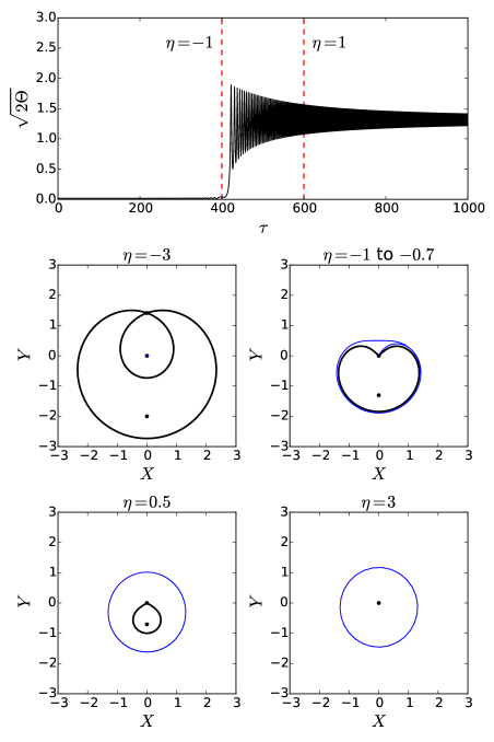
Figure 2: Resonant passage for $d\eta/d\tau=10^{-2}$ and $\Theta_{0}=10^{-4}$. The top panel shows the dimensionless eccentricity ($\sqrt{2\Theta}\sim e/\sqrt{\epsilon}$) evolution as a function of time $\tau$, with the boundaries of the resonance ($\eta=\pm 1$) marked by red dashed lines. The bottom four panels show the phase-space trajectories for periods of time near certain $\eta$ values or within a range of $\eta$. The blue curves are trajectories of the system, and the black curves and dots mark the separatrices and fixed points. The planet is initially at a low-eccentricity state ($\eta=-3$); it experiences a non-adiabatic “jump” near $\eta=-1$, and subsequent adiabatic evolution ($\eta=0.5$ and $\eta=3$) during which the phase-space area of the trajectory is conserved.

As $d\eta/d\tau$ increases, the final planet eccentricity $e_{\rm f}$ after resonance passage becomes smaller than $e_{\rm f,max}$. Figure 3 shows our numerical results of $\sqrt{2\Theta_{\rm f}}\sim e_{\rm f}/\sqrt{\epsilon}$ as a function of $d\eta/d\tau$ for several values of $\Theta_{0}$. Clearly, the eccentricity excitation can be significantly reduced when $d\eta/d\tau$ is too large. The critical value, $(d\eta/d\tau)_{c}$, above which $e_{\rm f}$ becomes less than $e_{\rm f,max}/2$, is of order $0.1$, but depends on the initial $\Theta_{0}$, and is smaller for smaller $\Theta_{0}$. This behavior can be qualitatively understood from Eq. (48), which shows that the libration period for an initially low-eccentricity trajectory is proportional to $|\ln\Theta_{0}|$. Thus, to achieve significant eccentricity excitation ($e_{\rm f}\mathrel{\raise 1.29167pt\hbox{$>$}\mkern-14.0mu\lower 2.58334pt\hbox{$\sim$}}e_{\rm f,max}/2$) in a resonance passage, we require

$$\left|{d\eta\over d\tau}\right|\mathrel{\raise 1.29167pt\hbox{$<$}\mkern-14.0mu\lower 2.58334pt\hbox{$\sim$}}{1\over|\ln\Theta_{0}|}.$$ (53)

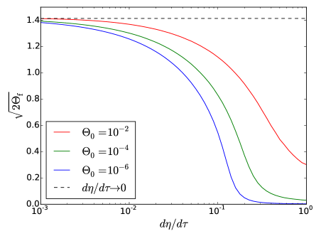
Figure 3: Final eccentricity ($\sqrt{2\Theta_{\rm f}}\sim e_{\rm f}/\sqrt{\epsilon}$) generated in a resonance passage as a function of $d\eta/d\tau$ for different values of initial eccentricity $\Theta_{0}$. The dashed line marks the theoretical value for the maximum eccentricity excitation (achieved for $d\eta/d\tau\to 0$), as calculated in Eq. (52)

3.2 Decreasing $\eta$: Resonance Trapping

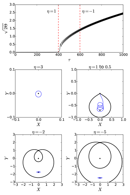
Figure 4: Resonant trapping for $d\eta/d\tau=-10^{-2}$ and $\Theta_{0}=10^{-4}$ (cf. Fig. 2). The planet is initially in a low-eccentricity state ($\eta=3$). At $\eta\leq 1$, a libration (resonance) zone bifurcates from the origin, and the planet gets trapped in the resonance ($\eta=1$-$0.5$). As $\eta$ continues to decrease, the trajectory “follows” the center (fixed point) of the resonance ($\eta=-2$ and $-5$) with ever increasing eccentricity.

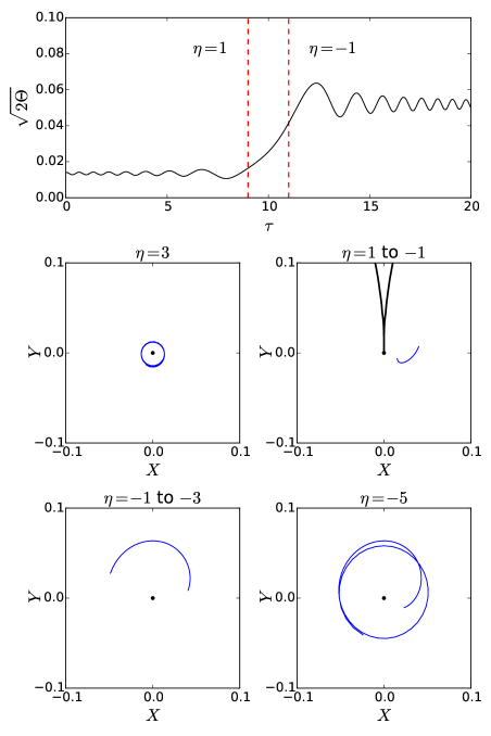
Figure 5: Same as Fig. 4, but with $d\eta/d\tau=-1$ and $\Theta_{0}=10^{-4}$. The axes for eccentricity evolution and phase space trajectories are zoomed-in to show the small eccentricity. During $1>\eta>-1$ the eccentricity grows as a result of the fast changing $\eta$. The system is not trapped into resonance; the phase-space trajectory always circulates around the origin.

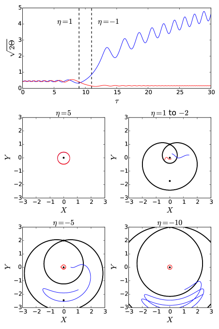
Figure 6: Same as Fig. 4, but with $d\eta/d\tau=-1$ and $\Theta_{0}=10^{-1}$ (a large $\Theta_{0}$ is chosen to better visualize the difference between the two cases). The blue and red curves correspond to two systems that differ only by $\pi/2$ in the initial phase ($\theta$). One of the systems is trapped (blue), while the other is not (red). Trapping should be considered probabilistic in this regime, since the phase for a realistic system is arbitrary.

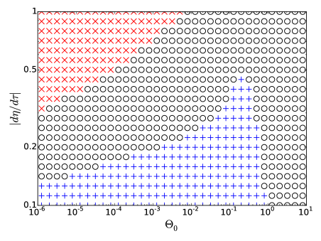
Figure 7: Resonance trapping condition in the $\Theta_{0}-|d\eta/d\tau|$ parameter space. Blue crosses: the system will be trapped with certainty. Red saltires: the system cannot be trapped. Black circles: the system can be trapped for some initial phase $\theta$; trapping is probabilistic in this case.

Consider a system initially at $\eta_{0}>1$ and $\Theta_{0}\ll 1$. The system passes through the resonance as $\eta$ gradually decreases. For $|d\eta/d\tau|\ll 1$, the planet will be trapped in resonance and its eccentricity can grow to large values. Figure 4 depicts an example. Initially, when $\eta>1$, the trajectory is circulating around the origin at a small eccentricity. As $\eta$ passes $1$, a separatrix emerges from the origin. This separatrix quickly expands and the trajectory falls into the resonant (libration) zone. The separatrix continues to expand as $\eta$ decreases, while the center of the resonance (the stable fixed point) moves to increasingly higher $\Theta$ value. The evolution is now fully adiabatic, and the trajectory is advected with the resonance to high eccentricity, conserving the its phase-space area. The mean eccentricity of the planet (as a function of $\eta$) is determined by the location of the stable fixed point inside the libration zone:

$${\bar{\Theta}}(\eta)=\frac{1-\eta}{2},$$ (54)

or

$${\bar{e}}(\eta)=\sqrt{{2\epsilon D\over C}{\bar{\Theta}}(\eta)}=\sqrt{{\epsilon D\over C}(1-\eta)}.$$ (55)

Once the system is captured in resonance, it will stay in resonance as $\eta$ continues to decrease, until the eccentricity becomes too large and the small-$e$ approximation breaks down. Note that the growth of ${\bar{e}}(\eta)$ is unbounded as $\eta$ keeps decreasing, suggesting that the planet will become unstable if the system stays in resonance long enough.

For larger values of $|d\eta/d\tau|$, the behavior of the system can be quite different. If $|d\eta/d\tau|$ is sufficiently large, the system passes through the resonance so fast that the eccentricity has little time to grow before $\eta$ falls below $-1$ and the trajectory ends up in the inner circulation zone, as is shown in Fig. 5. For a range of intermediate $|d\eta/d\tau|$ (this range depends on $\Theta_{0}$; see below), whether a system ends up trapped in resonance and follows the fixed point inside the libration zone, or remains circulating around $e=0$, depends on the phase $\theta$ when it enters resonance. Since this phase is random for realistic systems, the trapping should be considered probabilistic in this case. Figure 6 depicts an example of this “mixed” (probabilistic) behavior. Note that a larger $\Theta_{0}$ is chosen for this figure in order to better visualize both evolutionary trajectories (“trapped” vs “non-trapped”).

We have carried out numerical calculations for a wide range of $d\eta/d\tau$ and $\Theta_{0}$ values to determine the boundary between the three behaviors (trapping for certain, probabilistic trapping, trapping impossible) discussed above. The result is shown in Fig 7. Two trends are of interest here: First, for $\Theta_{0}\ll 1$, the $|d\eta/d\tau|$ values at the boundaries decrease as $\Theta_{0}$ decreases, suggesting that slower change of $\eta$ is required to trap a system with smaller $\Theta_{0}$. Second, around $\Theta_{0}\sim 1$, the probabilistic region quickly expands, and for larger $\Theta_{0}$ trapping becomes probabilistic even for small $|d\eta/d\tau|$. The second trend can be understood using the result from Borderies & Goldreich (1984), which shows that trapping become probabilistic for $\Theta_{0}\gtrsim 1$ in the $|d\eta/d\tau|\to 0$ regime. The first trend can be explained by noting that reaching adiabatic evolution before the system exits $\eta\in[-1,1)$ is a sufficient (but not necessary) condition for trapping; this can be used to approximate the lower boundary of the probabilistic trapping region. Specifically, to achieve adiabaticity before leaving the resonance requires $\Theta$ to reach a large enough value $\Theta_{\rm min}$ such that

$$\tau_{\rm lib}(\Theta_{\rm min})\sim-\ln\Theta_{\rm min}\lesssim\left|\frac{d\eta}{d\tau}\right|^{-1}.$$ (56)

Since $\Theta$ grows exponentially when it is small, we have

$$\ln\Theta_{\rm min}-\ln\Theta_{0}\sim\left|\frac{d\eta}{d\tau}\right|^{-1}.$$ (57)

Substituting this into (56) gives

$$\left|\frac{d\eta}{d\tau}\right|\lesssim\frac{1}{|\ln\Theta_{0}|}$$ (58)

as the condition of “certain” resonance trapping. Therefore, for $\Theta_{0}\ll 1$, the critical $|d\eta/d\tau|$ at which trapping becomes probabilistic should decrease as $\Theta_{0}$ decreases. Note that the condition (58) has the same scaling as Eq. (53) for the case of resonance passage, although the actual numerical results are different (see Figs. 3 and 7).

3.3 Timescales and Criteria for Eccentricity Excitation and Resonance Capture

The results of Sections 3.1-3.2 show that significant eccentricity excitation (i.e., $e_{\rm f}\gtrsim e_{\rm f,max}$ in the case of increasing $\eta$ or resonance capture in the case of decreasing $\eta$) requires $|d\eta/d\tau|\lesssim h^{-1}$, or

$$\begin{split}\left|\frac{d\eta}{dt}\right|^{-1}\gtrsim h\,T_{\rm res},\end{split}$$ (59)

where [see Eqs. (38)-(39)]

$$\begin{split}T_{\rm res}=\frac{na^{2}}{2|D|\Phi_{B0}}={T_{K}\over 2|D|}.\end{split}$$ (60)

The dimensionless quantity $h$ ranges from 1 to 100, depending on the initial eccentricity; see Figs. 3 and 7.

In various applications, the change of $\eta$ can result from the change one of the physical parameters of the systems, $X=\{a,a_{b},e_{b}\}$ [see Eq. (37)]. Since $|\partial\eta/\partial\ln X|\sim\epsilon^{-1}$, we find that, in order to have significant eccentricity excitation, the timescale for the variation of $X$ must satisfy

$$T_{X}\equiv\left|\frac{d\ln X}{dt}\right|^{-1}\gtrsim{h\over\epsilon}T_{\rm res}\equiv T_{\rm min}.$$ (61)

Obviously, this criterion is approximate. When $T_{X}$ is comparable to $T_{\rm min}$, numerical calculations are needed to determine the exact behavior of the system near resonance.

4 Applications to Circumbinary Planets

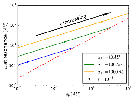
Figure 8: Semimajor axis $a$ of planet at the evection resonance as a function of $a_{b}$ for different $a_{B}$ values. All orbits are assumed to be circular, and $M_{1}=M_{2}=0.5M_{\odot},M_{B}=1M_{\odot}$. The dashed red line marks the inner boundary of the stability zone (see Eq. 62); the outer stability boundary is not shown because the lines for the resonance location always intersect the inner boundary first. The filled circles mark the location where $\epsilon=10^{-3}$ at resonance. We see that planets at resonance can be stable for a large range of realistic $a_{b},\,a_{B}$ values, and $\epsilon\geq 10^{-3}$ for some of the stable systems, allowing for appreciable eccentricity excitation even when there is no resonance trapping.

We now apply the results of previous sections to examine the effect of evection resonance on the evolution and stability of circumbinary planet in a stellar triple. The planet is unlikely to form at the resonant location due to the small width of resonance; however, it can be driven into the resonance due to secular effects such as planet migration and orbital decay of the inner binary. Passing through the resonance can make the planet’s orbit eccentric. In particular, eccentricity can be large if the planet is trapped in the resonance. This could lead to instability and ejection/destruction of the planet (Mudryk & Wu, 2006).

For a hierarchical triple system with circumbinary planet, the semi-major axis of the planet is restricted due to dynamical instability. Holman & Wiegert (1999) provided an empirical stability criterion: When all orbits are circular and coplanar, the planet’s orbit is stable only if

$$\begin{split}a_{b}(1.60+4.12q_{b}-5.09q_{b}^{2})\lesssim a\lesssim a_{B}(0.46-0.38q_{B}),\end{split}$$ (62)

where $q_{b}=M_{2}/M_{b}$ and $q_{B}=M_{B}/M_{\rm tot}$. Eccentric binary or planet orbits tend to make the stability zone narrower. Other empirical stability criteria are available (e.g., Mardling & Aarseth 2001), but we will use Eq. (62) as a guide.

For given binary separations $a_{b}$ and $a_{B}$, the evection resonance occurs at the planetary semi-major axis $a=a_{\rm res}$, given by [see Eq. (22)]

$$\begin{split}a_{\rm res}\simeq 0.92\,\left(1+{3e_{b}^{2}\over 2}\right)^{\!2/7}\!\!\left({\mu_{b}^{2}\over M_{b}M_{\rm tot}}\right)^{\!1/7}\!\!a_{b}^{4/7}a_{B}^{3/7}.\end{split}$$ (63)

Figure 8 shows the resonant planet location $a_{\rm res}$ as a function of $a_{b}$ for for different values of $a_{B}$. We see that $a_{\rm res}$ falls inside the stable region for a wide range of realistic $a_{b}$ and $a_{B}$ values.

As shown in Section 3.1, the maximum eccentricity the planet can attain in a resonance passage (without trapping) is of order $\sqrt{\epsilon}$. Evaluating Eq. (6) at $a=a_{\rm res}$, we find

$$\epsilon_{\rm res}\simeq 0.66\,\left(1+{3e_{b}^{2}\over 2}\right)^{\!\!10/7}\!{M_{B}\mu_{b}^{\!3/7}\over(M_{b}M_{\rm tot})^{5/7}}\left({a_{b}\over a_{B}}\right)^{\!6/7}.$$ (64)

(In the case of resonance trapping, a higher eccentricity can be achieved in principle if $\eta$ continues to decreases; see Section 3.2). Clearly, modest values of $\epsilon_{\rm res}$ (and thus $e_{\rm max}$ in a resonance passage) can be realized as long as $a_{B}$ is not too much larger than $a_{b}$.

As discussed in Section 3.3, in order to achieve resonance capture (when $\eta$ decreases) or significant eccentricity excitation in a resonance passage (when $\eta$ increases), the timescale for the variation of a relevant system parameter $X=\{a,a_{b},e_{b}\}$ must be longer than $T_{\rm min}$ [see Eq. (61)], i.e.,

$$T_{X}\gtrsim T_{\rm min}={h\over 2|D|}\left({M_{b}\mu_{b}\over M_{B}^{2}}\right)\left({a_{b}^{2}a_{B}^{6}\over a^{8}}\right){1\over n}.$$ (65)

Setting $a=a_{\rm res}$, we have

$$T_{\rm min}\simeq 0.213\,{h\over|D|}\left(1+{3e_{b}^{2}\over 2}\right)^{\!\!-13/7}{M_{b}^{10/7}M_{\rm tot}^{13/14}M_{\odot}^{1/2}\over\mu_{b}^{6/7}M_{B}^{2}}$$

$$\qquad~{}~{}\times\left(\frac{a_{b}}{1\text{AU}}\right)^{\!\!-12/7}\!\left(\frac{a_{B}}{100\text{AU}}\right)^{\!45/14}\text{Myr}.$$ (66)

4.1 Eccentricity Excitation During Inward Planet Migration

We first consider the effect of planet migration, with $\dot{a}\equiv da/dt<0$. This could result from planet interaction with gas discs (e.g. Goldreich & Tremaine 1980; Baruteau et al. 2014) or with planetesimal discs (e.g. Hahn & Malhotra 1999; Levison et al. 2007). The migration timescale $T_{\rm mig}=|a/\dot{a}|$ is highly uncertain, ranging from $<1$ Myrs to $>10$ Myrs.

Equation (37) shows that

$$\eta\sim{1\over\epsilon}\left(1-{n_{B}\over\dot{\varpi}}\right).$$ (67)

With $\dot{\varpi}\sim(\mu_{b}/M_{b})(a_{b}/a)^{2}n\propto a^{-7/2}$ [see Eq. (20)], we see that $\dot{a}<0$ leads to $\dot{\eta}=d\eta/dt>0$. Thus, the planet may experience eccentricity excitation without being captured into the resonance (Section 3.1). The maximum “final” eccentricity that can be attained is given by Eq. (52). Adopting a cononical set of parameters, $M_{1}=M_{2}=0.5M_{\odot}$, $M_{B}=1\,M_{\odot}$ and $e_{b}=I_{B}=0$, we find

$$e_{\rm f,max}=\sqrt{5\epsilon_{\rm res}}=1.05\left({a_{b}\over a_{B}}\right)^{\!3/7}.$$ (68)

The resonant planet semi-major axis is

$$a_{\rm res}=0.56\,a_{b}^{4/7}a_{B}^{3/7}.$$ (69)

The mimimum migration timescale required to achieve $e_{\rm f}\sim e_{\rm f,max}/2$ is

$$T_{\rm min}=3.55\left({h\over 10}\right)\left(\frac{a_{b}}{1\text{AU}}\right)^{\!\!-12/7}\!\left(\frac{a_{B}}{100\text{AU}}\right)^{\!45/14}\text{Myr},$$ (70)

where $h\sim 10$ (see Fig. 3).

Figure 9 shows the $a_{b}$-$a_{B}$ parameter space where eccentricity excitation due to resonance passage is possible. We see that an eccentricity $\gtrsim 0.2$ can be easily achieved for planets around short-period binaries ($a_{b}\lesssim 0.3$ AU). This requires that the external perturber is relatively close so that $a_{\rm res}$ lies not too far from the instability limit and that the migration timescale is sufficiently large.

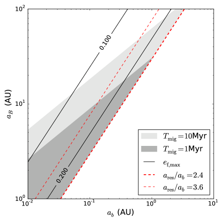
Figure 9: Parameter space (in terms of $a_{b}$ and $a_{B}$, the semimajor axes of the inner and outer binaries) for which significant eccentricity excitation occurs during inward planet migration. The system has $M_{1}=M_{2}=0.5M_{\odot}$, $e_{b}=0$, $M_{B}=1M_{\odot}$ and $I_{B}=0$. For given $a_{B}$ and $a_{b}$, the planet’s semimajor axis $a$ is taken as its value at resonance ($a_{\rm res}$). The black solid lines are level curves of constant $e_{\rm f,max}$ (the maximum eccentricity that can be attained due to resonance passage; see Eq. 68). In the dark (light) grey region, the planet can be excited to $e_{\rm f}\sim e_{\rm f,max}/2$ if the migration timescale ($T_{mig}$) is $1$ Myrs ($10$ Myrs) – This is determined by the condition $T_{\rm mig}>T_{\rm min}$ (see Eq. 70) with $h=10$. The lower red-dashed line indicates the inner stability boundary $a_{\rm res}/a_{b}\simeq 2.4$ (see Eq. 62).

Another factor that needs to be considered is eccentricity damping. While the planet migrates in the disc, its eccentricity may be damped by planet-disc interaction. Typically, the eccentricity damping timescale $T_{\text{dmp}}$ is much less than $T_{\text{mig}}$ (e.g., Kley & Nelson 2012). So for most systems discussed above, we actually have $T_{\text{dmp}}\lesssim T_{\text{min}}\lesssim T_{\rm mig}$. However, note that for our systems the timescale of eccentricity libration is $T_{\text{res}}=h^{-1}\epsilon T_{\text{min}}\lesssim 10^{-3}T_{\text{min}}$ for $h=10$ and $\epsilon\lesssim 10^{-2}$. This is also the timescale for eccentricity growth during the resonance passage. Thus, to achieve eccentricity excitation we only require $T_{\text{res}}\lesssim T_{\text{dmp}}$, which can be satisfied for most systems with $T_{\text{min}}\lesssim T_{\text{mig}}$.

We conclude that a circumbinary planet undergoing inward migration can experience eccentricity excitation when passing through the evection resonance. If the eccentricity at resonance is sufficiently large, the planet may suffer instability and be ejected. On the other hand, if the eccentricity at resonance is too small to cause instability, then the planet may survive with a final eccentricity after passing through the resonance, or its eccentricity may decay to a small value due to damping from the disc. The circumbinary planet Kepler-34b has a significant eccentricity, $e=0.18$ (Welsh et al., 2012), whose origin is unknown. Resonant eccentricity excitation would play a role if an apprpriate tertiary stellar companion existed during the earlier planet migration phase.

4.2 Resonance Trapping Around Shrinking Eccentric Binary

We consider a planet orbiting around an eccentric inner binary, which is undergoing orbital decay and circularization due to tidal dissipation. Such a decaying eccentric binary represents the final stage of the “Lidov-Kozai Shrinkage” of the inner binary, when the Lidov-Kozai oscillation (driven by the external binary companion) is suppressed by various short-range forces and the inner binary undergoes “pure” tidal decay (e.g. Fabrycky & Tremaine 2007; Muñoz & Lai 2015; see Section 4.3 below). Since the planet is strongly coupled to the inner binary [see Eqs. (6)-(7)], in the absence of resonance, the secular interaction between the inner binary and the planet ensures that the planet’s orbit remains cricular and aligned with the inner binary (Muñoz & Lai, 2015). We now examine how the evection resonance changes the planet’s eccentricity.

From Eq. (37) or (67), with $\dot{\varpi}\propto(2+3e_{b}^{2})a_{b}^{2}$ [see Eq. (20)], we see that as $a_{b}$ and $e_{b}$ decrease in time, the parameter $\eta$ also decreases in time. Thus an out-of-resonance planet could be captured into resonance as the inner binary shrinks/circularizes (see Section 3.2).

Figures 10 (for $e_{b}=0$) and 11 (for $e_{b}=0.8$) show the $a_{b}-a_{B}$ parameter space where resonance capture is certain or has significant probability (see Section 3.2). We characterize the orbital decay of the inner binary with a constant timescale $T_{\rm shrink}=|a_{b}/\dot{a}_{b}|$. Shrinking due to tidal dissipation tends to be slow, and many systems have $T_{\rm shrink}$ as large as a few Gyr. We see that for $T_{\rm shrink}\mathrel{\raise 1.29167pt\hbox{$>$}\mkern-14.0mu\lower 2.58334pt\hbox{$\sim$}}100$ Myr, the binary decay is sufficiently slow that resonance capture for the planet is likely for a wide range of $a_{b}$’s and $a_{B}$’s.

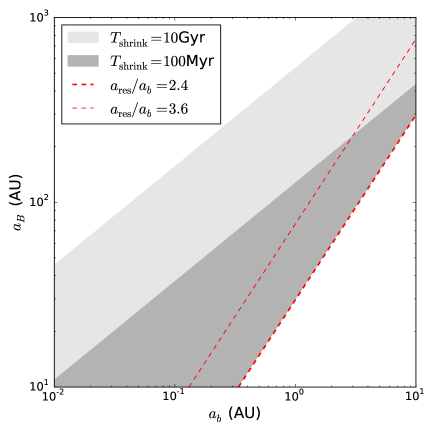
Figure 10: Similar to Fig. 9, except for the case of shrinking inner binary (with $e_{b}=0$ and $\dot{a}_{b}<0$). The lighter (dark) grey region indicates the parameter space where the planet can be trapped in the evection resonance when the the characteristic timescale of decrease in $a_{b}$ is $T_{\rm shrink}=10$ Gyr ($100$ Myr) – This is determined by the condition $T_{\rm shrink}>T_{\rm min}$ (see Eq. 70) with $h=10$. The lower red-dashed line indicates the inner stability boundary for the planet.

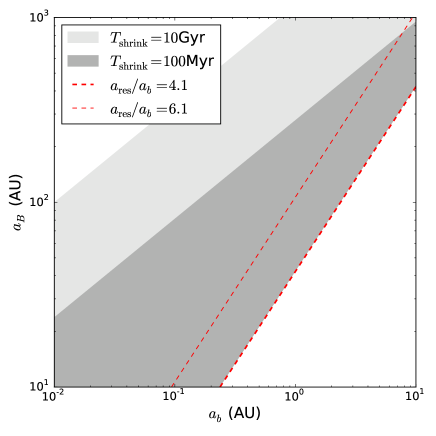
Figure 11: Same as Fig. 10, except for $e_{b}=0.8$. Note that the stability boundary also changes.

For given semi-major axes of the planet and outer binary, the resonance occurs at the inner binary separation (see Eq. 63)

$$a_{b,{\rm res}}\simeq 0.21\,\left(1+{3e_{b}^{2}\over 2}\right)^{\!-1/2}\!\left({M_{b}M_{\rm tot}\over 32\mu_{b}^{2}}\right)^{\!1/4}$$

$$\qquad\quad\times\left({a\over 1\,{\rm AU}}\right)^{\!7/4}\!\left({a_{B}\over 30\,{\rm AU}}\right)^{\!\!-3/4}.$$ (71)

Given the significant eccentricity excitation of the planet associated with resonance capture, the survival of the planet would likely require the initial binary $a_{b}$ to be less than $a_{b,{\rm res}}$, so that the resonance can be avoided.

4.3 Resonance Trapping During Lidov-Kozai Oscillation

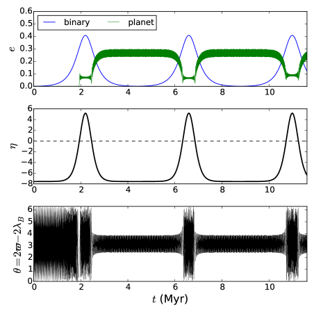
Figure 12: Evolution of the planetary eccentricity vector as the inner binary undergoes LK oscillations. The top panel shows the planet’s eccentricity together with the eccentricity of the inner binary, the middle panel shows the evolution of the resonance parameter $\eta$, and the bottom panel shows the evection resonance angle $\theta$. The system parameters are $M_{1}=M_{2}=0.5M_{\odot},\,M_{B}=1M_{\odot},a_{b}=1~{}\text{AU},a_{B}=~{}100\text{AU}$ and $a=4.2~{}\text{AU}$. The initial inner-outer binary inclination is $I_{B,0}=45^{\circ}$, which gives a maximum inner binary eccentricity of $e_{b,\text{max}}=0.408$. The planet is trapped in resonance when the eccentricity of the inner binary is low, and is out of resonance when $e_{b}$ is high.

We now study the evolution of the planet’s orbit when the inner binary undergoes Lidov-Kozai (LK) oscillation in eccentricity and inclination driven by the external binary. This problem has been studied by Muñoz & Lai (2015) using secular theory (see also Martin, Mazeh & Fabrycky 2015, Hamers, Perets & Portegies Zwart 2016), without including the effect of the evection resonance. Because of the strong coupling between the planet and the inner binary, we can assume that the orbital axes of the planet and the inner binary are always aligned (see (Muñoz & Lai, 2015)). For simplicity, here we neglect tidal dissipation and short-range forces in the inner binary, and we also assume that the planet’s mass is sufficiently small and thus does not influence the LK oscillation of the inner binary.

With these simplifying assumptions, the inner binary undergoes “pure” LK oscillation in $e_{b}$ and $I_{B}$ when the initial inclination angle $I_{B,0}$ is greater than $\cos^{-1}\sqrt{3/5}\simeq 39.2^{\circ}$. The oscillation period is of order $T_{\rm K,b}$, given by (recall that $n_{b}$ is the mean motion of the inner binary)

$$T_{\text{K,b}}={n_{b}a_{b}^{2}\over{\mathcal{G}}M_{B}a_{b}^{2}/a_{B}^{3}}={M_{b}\over M_{B}}\left({a_{B}\over a_{b}}\right)^{3}{1\over n_{b}}.$$ (72)

In each LK cycle, the inclination oscillates between $I_{B,0}$ and $I_{B,{\rm max}}=39.2^{\circ}$, while the eccentricity oscillates between $e_{b,0}\simeq 0$ and $e_{b,{\rm max}}$, with $(1-e_{b}^{2})^{1/2}\cos I_{B}$ conserved. The maximum inner binary eccentricity is given by

$$e_{b,\text{max}}=\sqrt{1-{5\over 3}\cos^{2}I_{B,0}}.$$ (73)

[See Fabrycky & Tremaine (2007) and Liu, Muñoz & Lai (2015) for a detailed discussion of how various short-range forces affect the LK oscillation.] Note that $I_{B,{\rm max}}$ is the inclination at $e_{b,\text{max}}$ and $I_{B,{\rm max}}<I_{B,0}$.

As $e_{b}$ oscillates in the LK cycle, the apsidal precession rate of the planet also oscillates between $\dot{\varpi}_{0}$ and $\dot{\varpi}_{\rm max}$, given by [see Eq. (20)]

$$\dot{\varpi}_{0}={3\Phi_{b0}\over 4a^{2}n},\qquad\dot{\varpi}_{\rm max}=\dot{\varpi}_{0}\left(1+{3e_{b,{\rm max}}^{2}\over 2}\right).$$ (74)

Thus, the planet will encounter the evection resonance during the LK cycle if $\dot{\varpi}_{0}<n_{B}<\dot{\varpi}_{\rm max}$, or

$$\begin{split}1<{n_{B}\over\dot{\varpi}_{0}}<1+{3e_{b,\text{max}}^{2}\over 2}.\end{split}$$ (75)

This implies that, for given parameters for the stellar triple ($a_{b}$, $a_{B}$ and stellar masses), resonance encounter occurs only for a restricted range of planetary semimajor axis, i.e.,

$$1<{a\over a_{\rm res,0}}<\left(1+{3e_{b,{\rm max}}^{2}\over 2}\right)^{\!2/7},$$ (76)

where $a_{\rm res,0}$ is given by Eq. (63) with $e_{b}=0$. For a given $a$ in this range, the resonance occurs at the inner binary eccentricity $e_{b,{\rm res}}$, given by

$${n_{B}\over\dot{\varpi}_{0}}=1+{3e_{b,\text{res}}^{2}\over 2}.$$ (77)

When the condition (75) is satisfied, the planet will pass the resonance twice in each LK cycle: (i) During the increasing-$e_{b}$ phase, $\eta$ changes from from $\eta_{0}\equiv\eta(e_{b}=0)<0$ to $\eta_{\rm max}\equiv\eta(e_{b}=e_{b,\text{max}})>0$; this can excite the planet’s eccentricity (if the initial eccentricity is small) but does not lead to resonance capture. (ii) During the decreasing-$e_{b}$ phase, $e_{b}$ passes the resonance for the second time, and $\eta$ decreases from $\eta_{\rm max}>0$ to $\eta_{0}<0$; this can lead to resonance capture. From Eq. (37), we find

$$\eta_{0}\simeq{4\over 5(1+\cos I_{B,0})^{2}\epsilon}\left(1-{n_{B}\over\dot{\varpi}_{0}}\right)=-{6e_{b,\text{res}}^{2}\over 5(1+\cos I_{B,0})^{2}\epsilon},$$ (78)

and

$$\eta_{\rm max}\simeq{6(e_{b,\text{max}}^{2}-e_{b,\text{res}}^{2})\over 5(1+\cos I_{B,\text{max}})^{2}\epsilon}.$$ (79)

Figure 12 shows an example of the evolution of the planetary eccentricity as the inner binary undergoes LK oscillation. We see that, except for the initial phase of the calculation, the planet spends most of the time in the trapped resonance (librating) state during the low-$e_{b}$ phase of the LK oscilation. It is thrown out the resonance only during the brief high-$e_{b}$ phase, as the system crosses $\eta=1$ and the area of the libration zone shrinks to zero. The mean eccentrcity of the planet in the trapped state, ${\bar{e}}_{\rm trap}$, can be estimated from Eq. (55), where $\eta$ is evaluated at $e_{b}=0$. We then have ${\bar{e}}_{\rm trap}={\bar{e}}(\eta=\eta_{0})$ given by

$${\bar{e}}_{\rm trap}\simeq\left[\frac{3}{4}e_{b,\text{res}}^{2}+{5\epsilon\over 8}(1+\cos I_{B,0})^{2}\right]^{1/2}\simeq{\sqrt{3}\over 2}\,e_{b,\text{res}}.$$ (80)

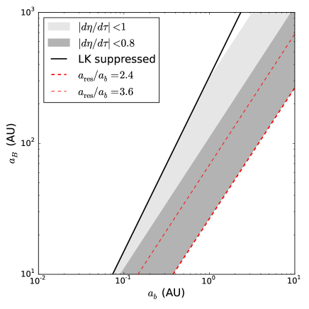
Figure 13: Parameter space (in terms of $a_{b}$ and $a_{B}$, the semi-major axes of the inner and outer binaries) for which resonance trapping can happen when the inner binary undergoes LK oscillations. Dark grey: $|\dot{\eta}|<0.6$. Light grey: $|\dot{\eta}|<1$. Thick red line: $a_{\rm res}/a_{b}=2.4$ (the stability limit). Thick black line: $T_{\rm GR}=T_{\rm K,b}$ (above this line, the short-range force due to GR can fully suppress LK oscillations of the inner binary). We see that $|d\eta/d\tau|\sim 1$ in most of the allowed parameter space. Our analysis (see text) shows that the system can be trapped in resonance in most cases.

As discussed at the beginning of Section 4, resonance capture requires that the LK timescale of the inner binary $T_{\rm K,b}$ (see Eq. 72) be not much smaller than $T_{\rm min}$ (see Eq. 66). For systems of interest here, we find $T_{\rm K,b}$ is of the same order as $T_{\rm min}$. More precisely, in light of the result of Section 3.2 (especially Fig. 7), we can evaluate $d\eta/d\tau$ at resonance using the exact equations for the $e_{b}$ and $I_{B}$ oscillations of the inner binary. Figure 13 shows the parameter space (in terms of $a_{b}$ and $a_{B}$) where $|d\eta/d\tau|<1$ can be realized. Note that in addition to the stabililty requirement for the planet, we also restrict to the $a_{b}$-$a_{B}$ space where LK osicllations are not suppressed by General Relativity (GR). This requres that $T_{\rm K,b}$ be shorter than the GR-induced apsidal precession timescale of the inner binary, i.e.,

$$T_{\rm K,b}\lesssim T_{\rm GR}={ac^{2}\over 3n_{b}\mathcal{G}M_{b}}.$$ (81)

In the example depicted in Fig. 12, the planet attains a significant eccentricity in the first ($\eta$-increasing) resonance passage (during the first half of the LK cycle). The $\Theta$ value when the planet crosses the resonance again (during the $\eta$-decreaisng phase) can be $\sim 1$. From Fig. 7 we see that the planet can be trapped into resonance for $|\dot{\eta}|\sim 1$ if $\Theta$ is large enough when the system enters resonance. This explains why the system can be trapped in resonance despite having $|d\eta/d\tau|\sim 1$.

4.4 N-Body Calculations

To test the validity of the results discussed in Section 4.3, we have performed a N-body integration using the Mercury code (Chambers, 1999). The result is shown in Figure 14. The parameters are the same as the system depicted in Fig. 12, with initial inner binary eccentricity $e_{b}=e=10^{-3}$. The planet and binary eccentricities are evaluated by calculating the eccentricity vectors (Laplace-Runge-Lenz vectors) of the bodies. Due to the perturbation from the inner binary, the initial eccentricity of the planet exhibits small oscillations (with an amplitude $\sim 10^{-2}$) even before any resonance encounter; this does not occur in the secular approximation, when the planet and the inner binary are orbit-averaged. Because of this forced initial eccentricity, the excited eccentricity of the planet during the increasing-$\eta$ resonant passage is larger than the “secular” result shown in Fig. 12. The eccentricity libration amplitude when the system is captured in resonance is also slightly larger due to the increased phase space area of the trajectory. Besides these small differences, our N-body result agrees well with the result obtained from the integration of orbit-averaged equations as depicted in Fig. 12. During the third LK cycle of the binary, the planet fails to be captured into resonance as $\eta$ decreases below 0 (see Fig. 14), showing the probabilistic nature of trapping in this regime. Note that for Fig. 12 trapping is also probabilistic; the absence of non-trapping passage is a coincidence.

We see from Fig. 14) that, during the first $\sim 10$ Myr of the integration (the first three-four LK cycles), the planet is stable although both $e_{b}$ and $e$ can be significant. This stability arises because when $e$ reaches the maximum value due to resonance trapping, $e_{b}$ is always near its minimum. However, the planet becomes unstable when it passes resonance with increasing $\eta$ for the fourth time; this time the eccentricity excitation happens to be slightly larger, because the system fails to be trapped in the previous decreasing $\eta$ passage. This slightly larger $e$, together with the large $e_{b}$, makes the system unstable and the planet is ejected.

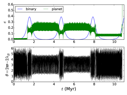
Figure 14: N-body integration for the system depicted in Fig. 12. The planet attains a large eccentricty at $t\sim 11$ Myr and is ejected.

5 Application to Multiplanet Systems

We now apply the theory of evection resonance (Sections 3 and 4) to multiplanet systems with external binary companions. This problem has been studied recently by (Touma & Sridhar, 2015). Our goal here is to adapt the results of previous sections to determine the explicit conditions for efficient excitation of planetary eccentricities.

Consider a wide binary where the primary hosts two planets, one of them much more massive than the other. Let the primary, the binary companion and the massive planet have mass $M_{\star}$, $M_{B}$ and $m_{p}$ respectively ($m_{p}\ll M_{\star}$); let the massive planet have semi-major axis $a_{p}$ and zero eccentricity, and the small planet, considered as a test mass, have semi-major axis $a$ and eccentricity $e$. As in the circumbinary planet problem, we assume that the planets are coplanar, while the outer binary can have an arbitrary inclination angle $I_{B}$ relative to the planetary orbits. The small planet undergoes apsidal precession caused by the quadrupole moment of the massive planet. Evection resonance occurs when apsidal precession frequency ($\dot{\varpi}$) equals $n_{B}$, the mean motion of the binary. During migration, $\dot{\varpi}$ changes due to the evolution of the planet’s semi-major axes, and the system may pass through evection resonance.

5.1 Inner Massive Planet

First consider the case when the inner planet is massive ($a_{p}<a$). In this regime we can directly apply the previous results for circumbinary planet by changing $(M_{1},M_{2},a_{b},e_{b})$ to $(M_{\star},m_{p},a_{p},e_{p})$ and taking $e_{p}=0$. We use $\Phi_{p}$ to denote the quadrupole perturbation potential of the massive planet (see Eq. 2) and define $\Phi_{p0}$ analogously, i.e. $\Phi_{b0}={\mathcal{G}}m_{p}a_{p}^{2}/a^{3}$. This is a rather approximate model, since we expand in $a_{p}/a$ and only keep the first nontrivial term in the perturbing potential. However, this model should be adequate to capture the qualitative behavior and scalings of the system.

To model the effect of planet migration we assume that the massive planet has a fixed semi-major axis $a_{p}$ (and eccentricity $e_{p}=0$), while the outer (small) planet migrates inward or outward with a constant rate $|{\dot{a}}/a|\equiv T_{\rm mig}^{-1}$. Since the apsidal precession rate $\dot{\varpi}\propto a^{-7/2}$, we have $\partial\eta/\partial a<0$ (see Eq. 37). Thus, for slow migration, $\eta$ increases as the outer planet migrates inward, leading to resonance passage and eccentricity excitation (see Section 3.1), and $\eta$ decreases as the planet migrates outward, leading to resonance trapping (Section 3.2).

The typical timescale of migration driven by gas in the disc can range from $<1$ Myrs to $>10$ Myrs, while outward migration due to scatterings with planetesimals occurs on longer timescales (100’s Myrs). The result of Section 3 (see Eq. 61 or Eq. 66) shows that to ensure eccentricity excitation or resonance capture the migration time must satisfy (with $e_{p}=0$)

$$T_{\rm mig}\mathrel{\raise 1.29167pt\hbox{$>$}\mkern-14.0mu\lower 2.58334pt\hbox{$\sim$}}T_{\rm min}\simeq 767\,{h\over|D|}\left({m_{p}\over M_{J}}\right)^{\!\!-6/7}\left({M_{\star}^{20}M_{\rm tot}^{13}\over M_{B}^{28}M_{\odot}^{5}}\right)^{\!\!1/14}$$

$$\qquad\qquad\qquad\times\left(\frac{a_{p}}{1\text{AU}}\right)^{\!\!-12/7}\!\left(\frac{a_{B}}{200\text{AU}}\right)^{\!45/14}\text{Myr},$$ (82)

where $M_{\rm tot}=M_{\star}+M_{B}$, and we have set $a=a_{\rm res}$ (the resonance semi-major axis of the planet), with

$$a_{\rm res}\simeq 1.2\left({m_{p}\over 1\,M_{J}}\right)^{\!\!2/7}\!\left({M_{\odot}^{2}\over M_{\star}M_{\rm tot}}\right)^{\!\!1/7}\!\left({a_{p}\over 1\,{\rm AU}}\right)^{\!4/7}\!\left({a_{B}\over 200\,{\rm AU}}\right)^{\!3/7}{\rm AU}.$$ (83)

Figure 15 shows the region in $a_{p}$-$a_{B}$ parameter space where resonance trapping (for outward migration) or eccentricity excitation comparable to $e_{\rm f,max}$ (for inward migration) is possible. From Eq. (52) we find that the maximum eccentrcity that can be achieved in a resonance passage is given by (see also Eq. 64)

$$e_{\rm f,max}=\sqrt{2\epsilon_{\rm res}D\over C}$$

$$\quad\simeq 0.042\left({m_{p}\over 1\,M_{J}}\right)^{\!3/14}\!{M_{B}^{1/2}M_{\odot}^{3/14}\over(M_{\star}M_{\rm tot})^{5/14}}\left({200a_{p}\over a_{B}}\right)^{\!3/7},$$ (84)

where we have used $2D/C=5$ (for $e_{p}=I_{B}=0$). We see that for inward migration, only modest eccentricity ($e_{\rm f,max}\lesssim 0.1$) can be attained in a resonance passage. The reason is that $\epsilon$ is quite small for any binary companion that induces resonance on the (small) planet which satisfies the stability criterion. For outward migration, the region in the parameter space where the system can be trapped in resonance is much larger, since the timescale can be larger for outward migration driven by planetesimal scatterings. Also note that in this case, the eccentricity excitation for a system trapped in resonance is not limited by the small value of $\epsilon$ (see Eq. 55).

Note $T_{\rm min}$ depends on the planet mass. Figure 15 uses $m_{p}=10\,M_{J}$ and solar-mass stars. For smaller planet mass, the region allowing resonance trapping shrinks. For example, at $m_{p}=1\,M_{J}$, no system with $T_{\rm mig}\lesssim 250$ Myr and $a_{p}>0.01$ AU allows trapping if we take $h=10$. Therefore, resonance trapping only occurs for the most massive planets.

Touma & Sridhar (2015) studied similar systems in greater detail. Here we compare their result with ours. The canonical system considered by Touma & Sridhar has $m_{p}\simeq 10\,M_{J}$, $a_{p}=5$ AU, $a_{B}=1000$ AU and $T_{\rm mig}\simeq 220$ Myr. As shown in Fig. 15, this system lies far outside the region in which we consider trapping likely, and yet Touma & Sridhar found resonance trapping in their calculations. This difference arises because we use $h=10$ in Fig. 15 (i.e. we require $|d\eta/d\tau|<0.1$ for effective trapping; see Sections 3.2-3.3), which is appropriate for the (scaled) initial eccentricity $\Theta_{0}\ll 1$. On the other hand, Touma & Sridhar chose a relatively large initial eccentricity, $e_{0}\simeq 0.05$, corresponding to $\Theta_{0}\sim 1$. As discussed in Section 3.2 (see Fig. 7), for $\Theta_{0}\mathrel{\raise 1.29167pt\hbox{$>$}\mkern-14.0mu\lower 2.58334pt\hbox{$\sim$}}1$, the system is in the probabilistic trapping regime with nontrivial trapping probability.

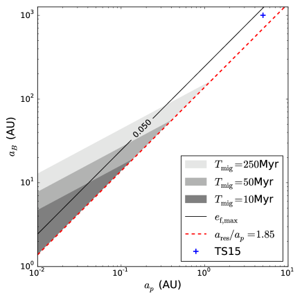
Figure 15: Parameter space (in terms of $a_{p}$ and $a_{B}$, the semi-major axes of the massive planet and the external binary) for which significant eccentricity excitation or resonance trapping occurs during the migration of a low-mass planet. The system has $M_{\star}=M_{B}=1M_{\odot}$, $m_{p}=10\,M_{\rm Jup}$ and $I_{B}=0$. The black solid line marks $e_{\rm f,max}=0.05$. The red-dashed line indicates the inner stability boundary $a_{\rm res}/a_{p}\simeq 1.85$, as given by the fitting formula of Petrovich (2015). In the three grey regions, the small planet can be excited to $e_{\rm f}\sim e_{\rm f,max}/2$ for inward migration or trapped in resonance for outward migration if the migration timescale ($T_{\rm mig}$) is $10$ Myrs, $50$ Myrs and $250$ Myrs respectively. This is determined by the condition $T_{\rm mig}\mathrel{\raise 1.29167pt\hbox{$>$}\mkern-14.0mu\lower 2.58334pt\hbox{$\sim$}}T_{\rm min}$ (see Eq. 82) with $h=10$ – as appropriate when the initial eccentricity $e_{0}$ is sufficiently small (such that $\Theta_{0}\ll 1$). The blue cross marks the canonical system considered by Touma & Sridhar (2015), which has $a_{p}=5$ AU and $a_{B}=1000$ AU (see text for discussion).

5.2 Outer Massive Planet

Next we consider the case when the massive planet is the outer planet ($a_{p}>a$). The potential from the massive planet ($m_{p}$) on the inner (small) planet is

$$\begin{split}\Phi_{p}=-\frac{\Phi_{p0}}{8}\left(2+3e^{2}\right),\end{split}$$ (85)

where

$$\begin{split}\Phi_{p0}=\frac{\mathcal{G}m_{p}a^{2}}{a_{p}^{3}}.\end{split}$$ (86)

The dimensionless ratio $\epsilon$ is

$$\begin{split}\epsilon=\frac{\Phi_{B0}}{\Phi_{p0}}=\frac{M_{B}a_{p}^{3}}{m_{p}a_{B}^{3}}\end{split}$$ (87)

Although $\Phi_{p}$ has a different dependence on $e$ compared to $\Phi_{b}$ (see Eq. 2), we can use the same procedure as in Section 2.2 to simplify the Hamiltonian. We obtain the same dimensionless Hamiltonian as Eq. (17), but with

$$A=-\frac{3}{4},~{}~{}~{}C=\frac{3}{8}$$ (88)

while $B,D$ are the same. The sign of $C$ differs from Eq. (20); thus in order to maintain the form of the scaled Hamiltonian $K$ (Eq. 26) while keeping $\Theta$ positive, the scaled variables/parameters need also be different:

$$\theta=-2\varpi+2\lambda_{B}+\pi,$$ (89)

$$\Theta=-\frac{C}{\epsilon D}\Gamma,$$ (90)

$$\eta=-\frac{A+\epsilon B+(n_{B}na^{2}/\Phi_{p0})}{\epsilon D}.$$ (91)

We can see that $\Theta\sim\epsilon^{-1}e^{2}$ still holds. One interesting property of the new variable $\theta$ (Eq. 77, as compared to Eq. 22) is that when a system is trapped in resonance ($\theta=\pi$), $\varpi-\lambda_{B}$ is 0 or $\pi$, i.e., the planet will be aligned or anti-aligned with the binary when the system is in resonance. This is in contrast to the situations studied in previous sections, where resonance corresponds $\varpi-\lambda_{B}=\pm\pi/2$.

The new $\eta$ (as a function of $A,B,C,D$) defined in Eq. (79) differs from Eq. (27) by a sign, and can be written as

$$\begin{split}\eta=\frac{4}{5(1+\cos I_{B})^{2}}\frac{1}{\epsilon}\left[\frac{n_{B}}{\dot{\varpi}(e=0)}-1+\frac{1}{2}\,\epsilon\,(1-3\cos^{2}I_{B})\right].\end{split}$$ (92)

Also note that the apsidal precession frequency is given by

$$\begin{split}\dot{\varpi}(e=0)=\frac{3}{4}\frac{\Phi_{p0}}{na^{2}}\propto a^{3/2}.\end{split}$$ (93)

Clearly, $\partial\eta/\partial a<0$. Thus, $\eta$ increases as the small planet migrates inward, leading to eccentricity excitation, and $\eta$ decreases as the planet migrates outward, leading to resonance trapping. The location of resonance, set by $n_{B}\simeq\dot{\varpi}(e=0)$, is given by

$$a_{\rm res}\simeq\left({16M_{\star}M_{\rm tot}\over 9m_{p}^{2}}\right)^{\!1/3}{a_{p}^{2}\over a_{B}}.$$ (94)

The corresponding $e_{\rm f,max}$ is

$$e_{\rm f,max}=\sqrt{2\epsilon|D|\over C}=\sqrt{20\epsilon}$$

$$\qquad\simeq 0.14\,\left({M_{B}\over 10^{3}m_{p}}\right)^{\!1/2}\left({100a_{p}\over a_{B}}\right)^{\!3/2},$$ (95)

where the second equality assumes $e_{p}=I_{B}=0$. The minimum migration timescale for efficient eccentricity excitation is

$$T_{\rm min}={h\over 2|D|}{M_{\star}m_{p}\over M_{B}^{2}}{a_{B}^{6}\over a^{3}a_{p}^{3}}{1\over n}$$ (96)

$$\qquad\simeq 54\,{h\over|D|}\!\left(\!{m_{p}\over M_{J}}\!\right)^{2}{M_{\odot}^{5/2}\over M_{B}^{2}M_{\rm tot}^{1/2}}$$

$$\qquad\qquad\times\left({a_{B}\over 100\,{\rm AU}}\right)^{\!15/2}\left({a_{p}\over 1\,{\rm AU}}\right)^{\!-6}{\rm Myr}.$$

Figure 16 shows the parameter space where nontrivial eccentricity excitation or resonance trapping occurs. We see that the qualitative behavior is similar to the inner massive planet case discussed in Section 5.1; the major difference is that the region allowing for significant eccentricity excitation or resonance trapping now lies almost parallel to the instability limit, and such difference is due to the difference of the scaling of $T_{\rm min}$. Although Eq. (96) suggests that $T_{\rm min}$ decreases as $m_{p}$ decreases, resonance trapping or significant eccentricity excitation is still less likely for smaller $m_{p}$. This is because smaller $m_{p}$ leads to smaller $a_{p}/a_{\rm res}$ and the system is more prone to instability. Moreover, since we require $a_{\rm res}<a_{p}$, resonance becomes impossible when $m_{p}$ is too small (see Eq. 85).

Together, Figures 15 and 16 show that the region where nontrivial eccentricity excitation occurs occupies a relatively small portion of the parameter space both inner/outer massive planet cases. This suggests that evection resonance plays only a modest role in most of the multiplanet systems with binary companions.

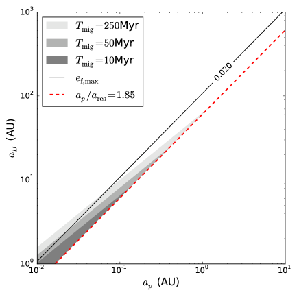
Figure 16: Similar to Fig. 15 except for the outer massive planet case ($a<a_{p}$). We see that the qualitative behavior is similar to the $a>a_{p}$ case, and the shape of the region for eccentricity excitation changes due to the different scaling relations.

6 Summary

We have developed an analytic theory of evection resonance for circumbinary planets and multiplanet systems under the perturbation from an external companion. The resonance occurs when the apsidal precession of the planet, driven by the quadrupole moment associated with the inner binary or another massive planet, equals the orbital frequency of the external perturber. The theory is quite general and can be applied to various astrophysical/planetary setups. The key results of our paper are:

1. The dynamics of a planet near the evection resonance is described by the one-parameter nondimensional Hamiltonian, Eq. (26). This Hamiltonian has the same form as that describing second-order mean-motion resonances.

2. As the parameter $\eta$ (see Eqs. 27-28) changes due to the long-term evolution of the system (e.g., planet migration or inner binary shrinkage), the planet may pass through the resonance (for increasing $\eta$) or experience resonance capture (for decreasing $\eta$). In the former case, the maximum planetary eccentricity that can be attained is given by Eq. (43); in the latter case, the eccentricity could continue to grow to larger values (as $\eta$ keeps decreasing) as long as the planet stays in resonance. (Resonance escape may occur when the eccentricity becomes “nonlinear” and the planet becomes unstable.) In both cases, in order to achieve appreciable eccentricity excitation (comparable to $e_{\rm f,max}$) or resonance capture, the dimensionless parameter $\eta$ must vary slowly (Eq. 49; see also Fig. 7), or equivalently, the timescale of variation for the dimensional system parameter (such as planetary or binary semi-major axis) must be longer than a minimum value (Eq. 52) which depends on the planet’s initial eccentricity.

3. Applying our theory to circumbinary planets with external stellar perturbers (Section 4), we show that: (i) Inward planetary migration may lead to resonance passage, producing eccentric planet. An example of such circumbinary planet is Kepler-34b, with $e=0.18$ (Welsh et al., 2012). (ii) The shrinkage of inner binary may result in resonance capture of the planet, potentially leading to its destruction. (iii) The planet may periodically enter and exit evection resonance as the inner binary undergoes Lidov-Kozai oscillations. Furthermore, our N-body calculations (Section 4.4) suggest that during this process the planet is likely to become unstable and be destructed due to its excited eccentricity. Taken together, our results suggest that survival of planet around a shrinking binary (Muñoz & Lai, 2015) likely requires that the initial binary semi-major axis to be less than a critical value, so that the evection resonance can be avoided (see Eq. 62).

4. Applying our theory to multiplanet systems with external stellar perturbers (Section 5), we clarify the conditions for significant eccentricity excitation due to evection resonance. We approximate a multiplanet system as consisting of a test-mass planet either inside or outside a massive planet. We find that the conditions for eccentricity excitation/capture are qualitatively similar for the two cases, despite the difference in scaling relations for the two different planetary architectures. In general, we find that the parameter space where nontrivial eccentricity excitation occurs is relatively small, suggesting that evection resonance plays only a modest role in most of the multiplanet systems with binary companions.

References

- Baruteau et al. (2014) Baruteau C. et al., 2014, Protostars and Planets VI, 667
- Borderies & Goldreich (1984) Borderies N., Goldreich P., 1984, Celestial mechanics, 32, 127
- Chambers (1999) Chambers J. E., 1999, MNRAS, 304, 793
- Doyle et al. (2011) Doyle L. R. et al., 2011, Science, 333, 1602
- Fabrycky & Tremaine (2007) Fabrycky D., Tremaine S., 2007, ApJ, 669, 1298
- Goldreich & Tremaine (1980) Goldreich P., Tremaine S., 1980, ApJ, 241, 425
- Hahn & Malhotra (1999) Hahn J. M., Malhotra R., 1999, AJ, 117, 3041
- Hamers, Perets & Portegies Zwart (2016) Hamers A. S., Perets H. B., Portegies Zwart S. F., 2016, MNRAS, 455, 3180
- Holman & Wiegert (1999) Holman M. J., Wiegert P. A., 1999, AJ, 117, 621
- Kley & Nelson (2012) Kley W., Nelson R. P., 2012, Annual Review of Astronomy & Astrophysics, 50, 211
- Kostov et al. (2015) Kostov V. B. et al., 2015, ArXiv e-prints
- Levison et al. (2007) Levison H. F. et al., 2007, Protostars and planets V, 1, 669
- Liu, Muñoz & Lai (2015) Liu B., Muñoz D. J., Lai D., 2015, MNRAS, 447, 747
- Mardling & Aarseth (2001) Mardling R. A., Aarseth S. J., 2001, MNRAS, 321, 398
- Martin, Mazeh & Fabrycky (2015) Martin D. V., Mazeh T., Fabrycky D. C., 2015, MNRAS, 453, 3554
- Muñoz & Lai (2015) Muñoz D. J., Lai D., 2015, PNAS, 112, 9264
- Mudryk & Wu (2006) Mudryk L. R., Wu Y., 2006, AJ, 639, 423
- Murray & Dermott (1999) Murray C. D., Dermott S. F., 1999, Solar system dynamics, Cambridge university press, pp. 321–408
- Peale (1986) Peale S., 1986, in IAU Colloq. 77: Some Background about Satellites, Vol. 1, pp. 159–223
- Petrovich (2015) Petrovich C., 2015, ApJ, 808, 120
- Spalding, Batygin & Adams (2016) Spalding C., Batygin K., Adams F. C., 2016, ApJ, 817, 18
- Touma & Wisdom (1998) Touma J., Wisdom J., 1998, AJ, 115, 1653
- Touma & Sridhar (2015) Touma J. R., Sridhar S., 2015, Nature, 524, 439
- Tremaine, Touma & Namouni (2009) Tremaine S., Touma J., Namouni F., 2009, AJ, 137, 3706
- Tremaine & Yavetz (2014) Tremaine S., Yavetz T. D., 2014, Am. J. Phys, American Journal of Physics, 769
- Welsh et al. (2012) Welsh W. F. et al., 2012, Nature, 481, 475