POMDP-lite for Robust Robot Planning under Uncertainty

Abstract

The partially observable Markov decision process (POMDP) provides a principled general model for planning under uncertainty. However, solving a general POMDP is computationally intractable in the worst case. This paper introduces POMDP-lite, a subclass of POMDPs in which the hidden state variables are constant or only change deterministically. We show that a POMDP-lite is equivalent to a set of fully observable Markov decision processes indexed by a hidden parameter and is useful for modeling a variety of interesting robotic tasks. We develop a simple model-based Bayesian reinforcement learning algorithm to solve POMDP-lite models. The algorithm performs well on large-scale POMDP-lite models with up to $10^{20}$ states and outperforms the state-of-the-art general-purpose POMDP algorithms. We further show that the algorithm is near-Bayesian-optimal under suitable conditions.

I INTRODUCTION

Imperfect robot control, sensor noise, and unexpected environment changes all contribute to uncertainties and pose significant challenges to robust robot planning. Robots must explore in order to gain information and reduce uncertainty. At the same time, they must exploit the information to achieve task objectives. The partially observable Markov decision process (POMDP) [8, 25] provides a principled general framework to balance exploration and exploitation optimally. It has found application in many robotic tasks, ranging from navigation [20], manipulation [7, 12] to human-robot interaction [14]. However, solving POMDPs exactly is computationally intractable in the worst case [16]. While there has been rapid progress on efficient approximate POMDP algorithms in recent years (e.g., [23, 13, 22, 24, 21]), it remains a challenge to scale up to very large POMDPs with complex dynamics.

The complexity of a POMDP lies in the system dynamics, partial observability, and particularly, the confluence of the two. We introduce POMDP-lite, a factored model that restricts partial observability to state variables that are constant or change deterministically. While this may appear restrictive, the POMDP-lite is powerful enough to model a variety of interesting robotic tasks:

• Unknown system parameters. A double-pendulum acrobot with link mass unknown a priori swings up to the standup configuration [3, 5].

• Unknown types. In autonomous driving, a robot vehicle encounters a human driver of unknown behavior at an uncontrolled traffic intersection [4]. In a human-robot collaborative task, the robot poses an object to the human according to unknown human preference [14].

• Unknown goals. An assistive agent helps a human cooking one of several dishes, without knowing the human’s intention in advance [6].

These tasks all require the robot to gather information on the unknown quantities from noisy observations, while achieving the task objective at the same time. They in fact belong to a special case, in which the hidden variables remain constant throughout. We mainly focus on this special case here.

Interestingly, the famous Tiger problem, which appeared in a seminal paper on POMDPs [8], also belongs to this special case, after a small modification. In Tiger, an agent stands in front of two closed doors. A tiger is behind one of the doors. The agent’s objective is to open the door without the tiger. In the POMDP model, the state is the unknown tiger position. The agent has three actions: open the left door (OL), open the right door (OR), and listen (LS). OL and OR produce no observation. LS produces a noisy observation, tiger left (TL) or tiger right (TR), each correct with probability $0.85$. Listening has a cost of $-1$. If the agent opens the door with no tiger, it gets a reward of $10$; otherwise, it incurs a penalty of $-100$. To perform well, the agent must decide on the optimal number of listening actions before taking the open action. While Tiger is a toy problem, it captures the essence of robust planning under uncertainty: trade off gathering information and exploiting the information to achieve the task objective. The original Tiger is a repeated game. Once the agent opens a door, the game resets with the tiger going behind the two doors with equal probability. We change it into a one-shot game: the game terminates once the agent opens a door. The one-shot game has a single state variable, the tiger position, which remains unchanged during the game, and thus admits a POMDP-lite model. The repeated game is a POMDP, but not a POMDP-lite.

(a) Tiger on the left

(b) Tiger on the right

Figure 1: A POMDP model for one-shot Tiger is transformed into a set of two MDPs. A node is labeled by a pair, representing a POMDP state and an observation. The start state has null observation and is labeled accordingly. The special terminal state is labeled as “END”. An edge is labeled by a triple, representing the action , the probability of reaching the next state with the action, and the reward.

A POMDP-lite is equivalent to a set of Markov decision processes (MDPs) indexed by a hidden parameter. The key idea for the equivalence transformation is to combine a POMDP state and an observation to form an expanded MDP state, and capture both POMDP state-transition uncertainty and observation uncertainty in the MDP transition dynamics. In the one-shot Tiger example, we form two MDPs indexed by the tiger position, left (L) or right (R) (Fig. 1). An MDP state is a pair, consisting of a POMDP state and an observation. For example, in the MDP with the tiger on the left, we have $(\text{L},\text{TL})$, which represents that the true tiger position is L and the agent receives the observation TL. If the agent takes the action LS, with probability $0.15$, we transit to the new state $(\text{L},\text{TR})$ and receives observation TR. See Section III for details of the general construction.

The equivalence enables us to develop an online algorithm for POMDP-lite through model-based Bayesian reinforcement learning (RL). If the hidden parameter value were known, our problem would simply become an MDP, which has well-established algorithms. To gather information on the unknown hidden parameter, the robot must explore. It maintains a belief, i.e., a probability distribution over the hidden parameter and follows the internal reward approach for model-based Bayesian RL [11, 26], which modifies the MDP reward function in order to encourage exploration. At each time step, the online algorithm solves an internal reward MDP to choose an action and then updates the belief to incorporate the new observation received. Our algorithm is simple to implement. It performs well on large-scale POMDP-lite tasks with up to $10^{20}$ states and outperforms the state-of-the-art general-purpose POMDP algorithms. Furthermore, it is near-Bayesian-optimal under suitable conditions.

II Related Work

POMDP planning has a huge literature (see, e.g., [8, 13, 25, 23, 13, 22, 24, 21] ). Our brief review focuses on online search algorithms. At each time step, an online algorithm performs a look-ahead search and computes a best action for the current belief only [19]. After the robot executes the action, the algorithm updates the belief based on the observation received. The process then repeats at the new belief for the next time step. Online search algorithms scale up by focusing on the current belief only, rather than all possible beliefs that the robot may encounter. Further, since online algorithms recompute a best action from scratch at each step, they naturally handle unexpected environment changes without additional overhead. POMCP [22] and DESPOT [24] are the fastest online POMDP algorithms available today. Both employ the idea of sampling future contingencies. POMCP performs Monte Carlo tree search (MCTS). It has low overhead and scales up to very large POMDPs, but it has extremely poor worst-case performance, because MCTS is sometimes overly greedy. DESPOT samples a fixed number of future contingencies deterministically in advance and performs heuristic search on the resulting search tree. This substantially improves the worst-case performance bound. It is also more flexible and easily incorporates domain knowledge. DESPOT has been successfully implemented for real-time autonomous driving in a crowd [2]. It is also a crucial component in a system that won the Humanitarian Robotics and Automation Technology Challenge (HRATC) 2015 on a demining task.

Instead of solving the general POMDP, we take a different approach and identify a structural property that enables simpler and more efficient algorithms through model-based Bayesian RL. Like POMDP-lite, the mixed observability Markov decision process (MOMDP) [15] is also a factored model. However, it does not place any restriction on partially observable state variables. It is in fact equivalent to the general POMDP, as every POMDP can be represented as a MOMDP and vice versa. The hidden goal Markov decision process (HGMDP) [6] and the hidden parameter Markov decision process (HiP-MDP) [5] are related to POMDP-lite. They both restrict partially observability to static hidden variables. The work on HGMDP relies on a myopic heuristic for planning, and it is unlikely to perform well on tasks that need exploration. The work on HiP-MDP focuses mainly on learning the hidden structure from data.

There are several approaches to Bayesian RL [1, 17, 27, 11]. The internal reward approach is among the most successful. It is simple and performs well in practice. Internal reward methods can be further divided into two main categories, PAC-MDP and Bayesian optimal. PAC-MDP algorithms are optimal with respect to the true MDP [9, 27, 26]. They provide strong theoretical guarantee, but may suffer from over exploration empirically. Bayesian optimal algorithms are optimal with respect to the optimal Bayesian policy. They simply try to achieve high expected total reward. In particular, the Bayesian Exploration Bonus (BEB) [11] algorithm achieves lower sample complexity than the PAC-MDP algorithms. However, BEB requires a Dirichlet prior on the hidden parameters. Our algorithm is inspired by BEB, but constructs the exploration bonus differently. It allows arbitrary discrete prior, a very useful feature in practice.

III POMDP-lite

III-A Definition

POMDP-lite is a special class of POMDP with a “deterministic assumption” on its partially observable variable, specifically, the partially observable variable in POMDP-lite is static or has deterministic dynamic. Formally we introduce POMDP-lite as a tuple $(X,\Theta,A,O,T,Z,R,\gamma)$, where $X$ is a set of fully observable states, $\Theta$ is the hidden parameter which has finite number of possible values: $\Theta=\{\theta_{1},\theta_{2},...,\theta_{N}\}$, the state space is a cross product of fully observable states and hidden parameter: $X\times\Theta=\{(x_{i},\theta_{j})|x_{i}\in X,\theta_{j}\in\Theta\}$. $A$ is a set of actions, $O$ is a set of observations. The transition function $T(x,\theta,a,x^{\prime},\theta^{\prime})=P(x^{\prime}|\theta,x,a)P(\theta^{\prime}|\theta,x,a)$ for $x,x^{\prime}\in X,\theta,\theta^{\prime}\in\Theta,a\in A$ specifies the probability of reaching state $(x^{\prime},\theta^{\prime})$ when the agent takes action $a$ at state $(x,\theta)$, where $\theta^{\prime}=\theta$ or $P(\theta^{\prime}|\theta,x,a)=1$ according to the “deterministic assumption”. The observation function $Z(x^{\prime},\theta^{\prime},a,o)=P(o|\theta^{\prime},x^{\prime},a)$ specifies the probability of receiving observation $o$ after taking action $a$ and reaching state $(x^{\prime},\theta^{\prime})$. The reward function $R(x,\theta,a)$ specifies the reward received when the agent takes action $a$ at state $(x,\theta)$. $\gamma$ is the discount factor.

In POMDP-lite, the state is unknown and the agent maintains a belief $b$, which is a probability distribution over the states. In each step, the agent takes an action $a$ and receives a new observation, the belief is updated according to Bayes’ rule, $b^{\prime}=\tau(b,a,o)$. The solution to a POMDP-lite is a policy $\pi$ which maps belief states to actions, i.e., $\pi(b)=a$. The value of a policy $\pi$ is the expected reward with respect to the initial belief $b_{0}$: $V^{\pi}(b_{0})=\mathrm{E}\big{[}\underset{t=0}{\overset{\infty}{\sum}}\gamma^{t}R(x_{t},\theta_{t},a_{t})\big{]}$, where $(x_{t},\theta_{t})$ and $a_{t}$ denote the state and action at time $t$. An optimal policy has the highest value in all belief states, i.e., $V^{*}(b)\geq V^{\pi}(b),\forall\pi,b$, and the corresponding optimal value function satisfies Bellman’s equation:

$$V^{*}(b) =\underset{a}{\max}\bigg{\{}\underset{x\in X,\theta\in\Theta}{\sum}b(x,\theta)R(x,\theta,a)$$

$$\qquad\qquad\qquad+\gamma\underset{o\in O}{\sum}P(o|b,a)V^{*}\big{(}\tau(b,a,o)\big{)}\bigg{\}}$$

III-B Equivalent Transformation to a Set of MDPs

In this section, we show an important property of POMDP-lite model that it is equivalent to a collection of MDPs indexed by $\theta$. A MDP model with parameter $\theta_{i}$ is a tuple $(S,A,T,R,\gamma,\theta_{i})$, where $S$ is a set of states, $A$ is a set of actions, $T(\theta_{i},s,a,s^{\prime})$ is the transition function, $R(\theta_{i},s,a)$ is the reward function, $\gamma$ is the discount factor.

Theorem 1

Let $\mathcal{H}=(X,\Theta,A,O,T,Z,R,\gamma)$ be a POMDP-lite model, where $\Theta=\{\theta_{1},\theta_{2},...,\theta_{N}\}$. It equals to a collection of MDPs indexed by $\theta$, $\mathcal{C}=\underset{\theta_{i}\in\Theta}{\bigcup}(S,A,T,R,\gamma,\theta_{i})$.

Figure 2: Graphic model for POMDP-lite (left) and the MDP model with parameter $\theta_{i}$ (right).

Proof:

To show the equivalence between $\mathcal{H}$ and $\mathcal{C}$, we first reduce $\mathcal{C}$ to $\mathcal{H}$. This direction is easy, we can simply treat $\theta_{i}$ as part of the state in a POMDP-lite model, the remaining part can become part of a POMDP-lite model without change. The more interesting direction is to reduce $\mathcal{H}$ to $\mathcal{C}$.

Let’s first consider the case when the value of $\theta$ remains constant. Given $\theta=\theta_{i}$, the POMDP-lite model becomes a MDP model with parameter $\theta_{i}$, which consists of the following elements: $(S,A,T,R,\gamma,\theta_{i})$. Where $S$ is the state space: $S=X\times\tilde{O}$, $\tilde{O}=O\cup\{null\}$, in which $null$ simply means no observation received. $A$ is the set of actions which is identical to the actions in the POMDP-lite model. The transition function $T(\theta_{i},s,a,s^{\prime})=P(x^{\prime},\tilde{o}^{\prime}|\theta_{i},x,\tilde{o},a)=P(\tilde{o}^{\prime}|\theta_{i},x^{\prime},a)P(x^{\prime}|\theta_{i},x,a)$ specifies the probability of reaching state $s^{\prime}$ after taking action $a$ at state $s$, where $P(x^{\prime}|\theta_{i},x,a)$ and $P(\tilde{o}^{\prime}|\theta_{i},x^{\prime},a)$ are the transition and observation probability function in the POMDP-lite model. The reward function $R(\theta_{i},s,a)=R(\theta_{i},x,a)$ specifies the reward received when the agent takes action $a$ at state $s$. $\gamma$ is the discount factor. The graphic model in Fig. 2 shows the relationship between POMDP-lite model and the corresponding MDP model with parameter $\theta_{i}$. Since the hidden parameter has finite number of values, a POMDP-lite can be reduced to a collection of MDPs indexed by $\theta$.

Then, we show that a simple extension allows us to handle the case when the value of the hidden variable changes deterministically. The key intuition here is that the deterministic dynamic of hidden variable does not introduce additional uncertainties into the model, i.e., given the initial value of hidden variable $\theta^{0}$, and the history up to any time step $t$, $h_{t}=\{x_{0},a_{0},x_{1},a_{1},...,x_{t-1},a_{t-1}\}$, the value of hidden variable can be predicted using a deterministic function, $\theta^{t}=\phi(\theta^{0},h_{t})$. Thus given the initial value of hidden variable $\theta^{0}=\theta^{0}_{i}$ and a deterministic function $\phi$, a POMDP-lite model can be reduced to a MDP model: $(S,A,T,R,\gamma,\theta^{0}_{i})$. Compared with the static case, the state here is further augmented by the history $h_{t}$ i.e., $s_{t}=(x_{t},\tilde{o}_{t},h_{t})$. The value of $\theta^{t}$ was fully captured by $s_{t}$, $\theta^{0}_{i}$ and $\phi$, $\theta^{t}=\phi(\theta^{0}_{i},s_{t})$. The rest of the MDP model is similar to the static case. In particular, the set of actions $A$ is identical to the POMDP-lite model, the transition function is $T(\theta^{0}_{i},s_{t},a_{t},s_{t+1})=P(\tilde{o}_{t+1}|\theta^{t+1},x_{t+1},a_{t})P(x_{t+1}|\theta^{t},x_{t},a_{t})$, the reward function is $R(\theta^{0}_{i},s_{t},a_{t})=R(\theta^{t},x_{t},a_{t})$, $\gamma$ is the discount factor. Since $\theta^{0}$ has finite number of values, a POMDP-lite can be reduced to a collection of MDPs indexed by $\theta^{0}$. ∎

III-C Algorithm

In this part, we present an efficient model based BRL algorithm for POMDP-lite. The solution to the BRL problem is a policy $\pi$, which maps a tuple $(belief,state)$ to actions, i.e., $a=\pi(b,s)$. The value of a policy $\pi$ for a belief $b$ and state $s$ is given by Bellman’s equation

$$V^{\pi}(b,s) =R(b,s,a)+\gamma\underset{b^{\prime},s^{\prime}}{\sum}P(b^{\prime},s^{\prime}|b,s,a)V^{\pi}(b^{\prime},s^{\prime})$$

$$=R(b,s,a)+\gamma\underset{s^{\prime}}{\sum}P(s^{\prime}|b,s,a)V^{\pi}(b^{\prime},s^{\prime})$$

Where $a=\pi(s,b)$, $R(b,s,a)=\underset{\theta_{i}}{\sum}R(\theta_{i},s,a)b(\theta_{i})$ is the mean reward function, $P(s^{\prime}|b,s,a)=\underset{\theta_{i}}{\sum}T(\theta_{i},s,a,s^{\prime})b(\theta_{i})$ is the mean transition function. The second line follows from the fact that belief update is deterministic, i.e., $P(b^{\prime}|b,a,o)=1$. The optimal Bayesian value function is

$$\begin{split}V^{*}(b,s)&=\underset{a}{\max}\bigg{\{}R(b,s,a)+\gamma\underset{s^{\prime}}{\sum}P(s^{\prime}|b,s,a)V^{*}(b^{\prime},s^{\prime})\bigg{\}}\end{split}$$ (1)

$a=\pi^{*}(b,s)$ is the optimal action that maximizes the right hand size. Like the optimal policy in the original POMDP-lite problem, the optimal Bayesian policy chooses actions not only based on how they affect the next state but also based on how they affect the next belief.

However, the optimal Bayesian policy is computationally intractable. Instead of exploring by updating the belief each step, our algorithm explores by explicitly modify the reward function. In other words, each state action pair will have a reward bonus based on how much information it can reveal. The reward bonus used by our algorithm is motivated by the observation that the belief gets updated whenever some information about the hidden parameter has been revealed, thus we use the $L_{1}$ divergence between two beliefs to measure the amount of information gain. The reward bonus is defined formally as follows:

Definition 1

When the belief is updated from $b_{i}$ to $b_{j}$, we measure the information gain by the $L_{1}$ divergence between $b_{i}$ and $b_{j}$, i.e., $\|b_{j}-b_{i}\|_{1}=\underset{\theta_{i}\in\Theta}{\sum}\big{|}b_{j}(\theta_{i})-b_{i}(\theta_{i})\big{|}$. Based on it, the reward bonus for $(s,a)$ is defined as the expected $L_{1}$ divergence between current belief $b$ and next belief $b_{s^{\prime}}$:

$$RB(b,s,a)=\beta\underset{s^{\prime}}{\mathrm{E}}\big{[}\|b_{s^{\prime}}-b\|_{1}\big{]}=\beta\underset{s^{\prime}}{\sum}P(s^{\prime}|b,s,a)\|b_{s^{\prime}}-b\|_{1}$$

where $\beta$ is the constant tuning factor, $b_{s^{\prime}}$ is the updated belief after observing $s^{\prime}$.

At each time step, our algorithm solves an internal reward MDP, $M=(S,A,T,\tilde{R},\gamma,b)$. It chooses action greedily with respect to the following value function

$$\begin{split}\tilde{V}^{*}(b,s)=\underset{a}{\max}\bigg{\{}\tilde{R}(b,s,a)+\gamma\underset{s^{\prime}}{\sum}P(s^{\prime}|b,s,a)\tilde{V}^{*}(b,s^{\prime})\bigg{\}}\end{split}$$ (2)

Where $\tilde{R}(b,s,a)=R(b,s,a)+RB(b,s,a)$, in which $RB(b,s,a)$ is the reward bonus term and it is defined in Definition 1. Other parts are identical to Equation 1 except that belief $b$ is not updated in this equation. We can solve it using the standard Value Iteration algorithms, which have time complexity of $O(|A||X|^{2}|\Theta|^{2})$. In this work, we are more interested in problems with large state space, thus we are using UCT [10], an online MDP solver, to achieve online performance. Details of our algorithm is described in Algorithm 1, in which $\tilde{Q}^{*}(b_{t},s_{t},a)=\tilde{R}(b_{t},s_{t},a)+\gamma\underset{s_{t+1}}{\sum}P(s_{t+1}|b_{t},s_{t},a)\tilde{V}^{*}(b_{t},s_{t+1})$.

Algorithm 1

1:$t\leftarrow 0,b_{t}\leftarrow b_{0},s_{t}\leftarrow s_{0}$ // initialize the values

2:$T\leftarrow$ Maximum Steps

3:while not end and $t<T$ do

4:   $a_{t}\leftarrow\operatorname*{arg\,max}_{a}\tilde{Q}^{*}(b_{t},s_{t},a)$ // greedily choose an action

5:   $(r_{t},s_{t+1})\leftarrow ExecuteAction(a_{t})$

6:   $b_{t+1}\leftarrow UpdateBelief(b_{t},s_{t+1})$ // update the belief

7:   $t=t+1$

8:end while

IV Analysis

Although our algorithm is a greedy algorithm, it actually performs sub-optimally only in a polynomial number of time steps. In this section, we present some theoretical results to bound the sample complexity of our algorithm. Unless stated otherwise, the proof of the lemmas in this section are deferred to the appendix. For a clean analysis, we assume the reward function is bounded in $[0,1]$.

IV-A Sample Complexity

The sample complexity measures the number of samples needed for an algorithm to perform optimally. We start with a definition of sample complexity on a state action pair $(s,a)$.

Definition 2

Given the initial belief $b_{0}$, target accuracy $\kappa$, reward bonus tuning factor $\beta$, we define the sample complexity function of $(s,a)$ as: $\zeta(s,a)=f(b_{0},s,a,\kappa,\beta)$, such that if $(s,a)$ has been visited more than $\zeta(s,a)$ times, starting from belief $b_{0}$, the corresponding reward bonus of visiting $(s,a)$ at the new belief $b^{\prime}$ is less than $\kappa$, i.e., $RB(b^{\prime},s,a)<\kappa$. We declare $(s,a)$ as known if it has been sampled more than $\zeta(s,a)$ times, and cease to update the belief for sampling known state action pairs.

The following is an assumption for our theorem to hold true in general. The assumption essentially says that the earlier you try a state-action pair, the more information you can gain from it. We give a concrete example to illustrate our assumption in Lemma 1.

Assumption 1

The reward bonus monotonically decreases for all state action pairs $(s,a)$ and timesteps $t$, i.e., $RB(b_{i},s,a)\geq RB(b_{i+1},s,a)$.

Now, we present our central theoretical result, which bounds the sample complexity of our algorithm with respect to the optimal Bayesian policy.

Theorem 2

Let the sample complexity of $(s,a)$ be $\zeta(s,a)=f(b_{0},s,a,\kappa,\beta)$, where $\beta=O\big{(}\frac{|S|^{2}|A|}{(1-\gamma)^{2}}\big{)}$, $\kappa=\epsilon(1-\gamma)$. Let $\mathcal{A}_{t}$ denote the policy followed by the algorithm at time $t$, and let $s_{t}$, $b_{t}$ be the corresponding state and belief. Then with probability at least $1-\delta$, $V^{\mathcal{A}_{t}}(b_{t},s_{t})\geq V^{*}(b_{t},s_{t})-4\epsilon$, i.e., the algorithm is $4\epsilon$-close to the optimal Bayesian policy, for all but

$m=O\bigg{(}\frac{\sum_{s,a}\zeta(s,a)}{\epsilon(1-\gamma)^{3}}\ln\frac{1}{\sigma}\ln\frac{1}{\epsilon(1-\gamma)}\bigg{)}$

time steps.

In other words, our algorithm acts sub-optimally for only a polynomial number of time steps.

Although our algorithm was primary designed for Discrete prior, Theorem 2 can be applied to many prior distributions. We apply it to two simple special classes, which we can provide concrete sample complexity bound. First, we show that in the case of independent Dirichlet prior, the reward bonus monotonically decreases and the sample complexity of a $(s,a)$ pair can be bounded by a polynomial function. This case also satisfies Assumption 1.

Lemma 1 (Independent Dirichlet Prior)

Let $n(s,a)$ be the number of times $(s,a)$ has been visited. For a known reward function and an independent Dirichlet prior over the transition dynamics for each $(s,a)$ pair, $RB(b,s,a)$ monotonically decreases at the rate of $O\big{(}1/n(s,a)\big{)}$, and the sample complexity function $f(b_{0},s,a,\kappa,\beta)=O\big{(}\frac{|S|^{2}|A|}{\kappa(1-\gamma)^{2}}\big{)}$.

The strength of our algorithm lies in its ability to handle Discrete prior. We use a very simple example (Discrete prior over unknown deterministic MDPs) to show this advantage, and we state it in the following lemma. The intuition behind this lemma is quite simple, after sampling a state action pair, the agent will know its effect without noise.

Lemma 2 (Discrete prior over Deterministic MDPs)

Let $b_{0}$ be a Discrete prior over deterministic MDPs, the sample complexity function $f(b_{0},s,a,\kappa,\beta)\leq 1$.

IV-B Proof of Theorem 2

The key intuition for us to prove our algorithm quickly achieves near-optimality is that at each time step our algorithm is $\epsilon$-optimistic with respect to the Bayesian policy, and the value of optimism decays to zero given enough samples.

The proof for Theorem 2 follows the standard arguments from previous PAC-MDP results. We first show that $V^{\mathcal{A}_{t}}(b_{t},s_{t})$ is close to the value of acting according to the optimal Bayesian policy, assuming the probability of escaping the known state-action set is small. Then we use the Hoeffding bound to show that this “escaping probability” can be large only for a polynomial number of time steps.

We begin our proof with the following lemmas. Our first lemma essentially says that if we solve the internal reward MDP using the current mean of belief state with an additional exploration bonus in Definition 1, this will lead to a value function which is $\epsilon$-optimistic to the Bayesian policy.

Lemma 3 (Optimistic)

Let $\tilde{V}^{*}(b,s)$ be the value function in our algorithm, $V^{*}(b,s)$ be the value function in Bayesian policy. if $\beta=O\big{(}\frac{|S|^{2}|A|}{(1-\gamma)^{2}}\big{)}$, then $\forall s$, $\tilde{V}^{*}(b,s)\geq V^{*}(b,s)-\epsilon$.

The following definition is a generalization of the “known state-action MDP” in [27] to Bayesian settings. It is an MDP whose dynamics (transition function and reward function) are equal to the mean MDP for $(s,a)$ pairs in $K$ (known set). For other $(s,a)$ pairs, the value of taking those $(s,a)$ pairs in $M_{K}$ is equal to the current $\tilde{Q}$ value estimate.

Definition 3

Given current belief is $b$, a set of $\tilde{Q}$ value estimate for each $(s,a)$ pair, i.e., $\tilde{Q}(b,s,a)=\tilde{R}(b,s,a)+\gamma\underset{s^{\prime}}{\sum}T(b,s,a,s^{\prime})\tilde{V}^{*}(b,s^{\prime})$, and a set $K$ of known $(s,a)$ pairs, i.e., $RB(b,s,a)<\epsilon(1-\gamma)$. We define the known state-action MDP, $M_{K}=(S\cup\{s_{0}\},A,T_{K},R_{K},\gamma)$, as follows. $s_{0}$ is an additional state, under all actions from $s_{0}$ the agent returned to $s_{0}$ with probability $1$ and received reward $0$. For all $(s,a)\in K$, $R_{K}(s,a)=R(b,s,a)$ and $T_{K}(s,a,s^{\prime})=T(b,s,a,s^{\prime})$. For all $(s,a)\notin K$, $R_{K}(s,a)=\tilde{Q}(b,s,a)$ and $T_{K}(s,a,s_{0})=1$.

Our final lemma shows that the internal reward MDP and the known state-action MDP have low error in the set of known $(s,a)$ pairs.

Lemma 4 (Accuracy)

Fix the history to the time step $t$, let $b_{t}$ be the belief, $s_{t}$ be the state, $K_{t}$ be the set of known $(s,a)$ pairs, $M_{K_{t}}$ be the known state-action MDP, $\pi_{t}$ be the greedy policy with respect to current belief $b_{t}$, i.e., $\pi_{t}=\operatorname*{arg\,max}_{a}\tilde{Q}(b_{t},s,a)$. Then $\tilde{V}^{\pi_{t}}(b_{t},s_{t})-V_{M_{K_{t}}}^{\pi_{t}}(b_{t},s_{t})\leq\epsilon$.

Now, we are ready to prove Theorem 2.

Proof:

Let $b_{t},s_{t},K_{t},M_{K_{t}},\pi_{t}$ be as described in Lemma 4. Let $T=1/(1-\gamma)\ln(1/\epsilon(1-\gamma))$, then $|V^{\pi_{t}}_{M_{K_{t}}}(b_{t},s_{t},T)-V^{\pi_{t}}_{M_{K_{t}}}(b_{t},s_{t})|\leq\epsilon$ (see Lemma 2 of [9]). Let $A_{K}$ denote the event that, a $(s,a)$ pair not in $K_{t}$ is generated when executing $\mathcal{A}_{t}$ starting from $s_{t}$ for $T$ time steps. We have

$$V^{\mathcal{A}_{t}}(b_{t},s_{t},T)\geq V^{\pi_{t}}_{M_{K_{t}}}(b_{t},s_{t},T)-P(A_{K})/(1-\gamma)^{2}$$

$$\geq V^{\pi_{t}}_{M_{K_{t}}}(b_{t},s_{t})-\epsilon-P(A_{K})/(1-\gamma)^{2}$$

$$\geq\tilde{V}^{\pi_{t}}(b_{t},s_{t})-2\epsilon-P(A_{K})/(1-\gamma)^{2}$$

$$\geq V^{*}(b_{t},s_{t})-3\epsilon-P(A_{K})/(1-\gamma)^{2}$$

The first inequality follows from the fact that $\mathcal{A}_{t}$ equals to $\pi_{t}$ unless $A_{K}$ occurs, and $\tilde{Q}(b,s,a)$ can be bounded by $1/(1-\gamma)^{2}$ since we can limit the reward bonus to $1/(1-\gamma)$ and still maintain optimism. The second inequality follows from the definition of $T$ above, the third inequality follows from Lemma 4, the last inequality follows from Lemma 3 and the fact that $\pi_{t}$ is precisely the optimal policy for the internal reward MDP at time $t$. Now, suppose $P(A_{K})<\epsilon(1-\gamma)^{2}$, we have $V^{\mathcal{A}_{t}}(b_{t},s_{t})\geq V^{\mathcal{A}_{t}}(b_{t},s_{t},T)\geq V^{*}(b_{t},s_{t})-4\epsilon$. Otherwise, if $P(A_{K})\geq\epsilon(1-\gamma)^{2}$, by Hoeffding inequality, this will happen no more than $\tilde{O}\bigg{(}\underset{s,a}{\sum}\zeta(s,a)T/\epsilon(1-\gamma)^{2})\bigg{)}$ time steps with probability $1-\delta$, where $\tilde{O}$ (.) notation suppresses logarithmic factors. ∎

V Experiments

To evaluate our algorithm experimentally, we compare it with several state of the art algorithms in POMDP literature. POMCP [22] and DESPOT [24] are two successful online POMDP planners which can scale to very large POMDPs. QMDP [28] is a myopic offline solver being widely used for its efficiency. SARSOP [13] is a state of the art offline POMDP solver which helps to calibrate the best performance achievable for POMDPs of moderate size. Mean MDP is a common myopic approximation of Bayesian planning, which does not do exploration. For SARSOP, POMCP and DESPOT, we used the software provided by the authors, with a slight modification on POMCP to make it strictly follow 1-second time limit for planning. For our algorithm and Mean MDP, a MDP needs to be solved each step. We use an online MDP solver UCT [10] with similar parameter settings used in POMCP. The reward bonus scalar $\beta$ used by our algorithm is typically much smaller than the one required by Theorem 2, which is a common trend for internal reward algorithms. We tuned $\beta$ offline before using it for planning.

TABLE I: Performance comparison on Rocksample and Battleship

	$RS(7,8)$	$RS(11,11)$	$RS(15,15)$	$RS(20,20)$	$BS(10,5)$	$BS(15,7)$
States $|X|$	$12,544$	$247,808$	$7,372,800$	$10^{8}$	$10^{13}$	$10^{20}$
Actions $|A|$	$13$	$16$	$20$	$25$	$100$	$225$
Observations $|O|$	$3$	$3$	$3$	$3$	$2$	$2$
QMDP	$17.55\pm 0.44$	$16.10\pm 0.40$	$-$	$-$	$-$	$-$
SARSOP	$\mathbf{21.47\pm 0.04}$	$\mathbf{21.56\pm 0.11}$	$-$	$-$	$-$	$-$
POMCP	$19.95\pm 0.23$	$20.11\pm 0.23$	$15.51\pm 0.23$	$12.11\pm 0.23$	$57.40\pm 0.19$	$119.33\pm 0.58$
DESPOT	$20.80\pm 0.22$	$21.12\pm 0.21$	$\mathbf{18.59\pm 0.43}$	$12.56\pm 0.38$	$56.34\pm 0.22$	$117.39\pm 0.88$
Mean MDP	$15.11\pm 0.17$	$11.64\pm 0.17$	$7.53\pm 0.16$	$6.96\pm 0.11$	$57.46\pm 0.17$	$122.60\pm 0.59$
POMDP-lite	$21.03\pm 0.21$	$\mathbf{21.52\pm 0.20}$	$\mathbf{18.63\pm 0.20}$	$\mathbf{16.81\pm 0.20}$	$\mathbf{58.16\pm 0.17}$	$\mathbf{127.12\pm 0.61}$

We first apply the algorithms on two benchmarks problems in POMDP literature, in which we demonstrate the scaling up ability of our algorithm on larger POMDPs. In $Rocksample(n,k)$ [23], a robot moving in an $n\times n$ grid which contains $k$ rocks, each of which may be good or bad with probability $0.5$ initially. At each step, the robot can move to an adjacent cell, or sense a rock. The robot can only sample the rock when it is in the grid which contains a rock. Sample a rock gives a reward of $+10$ if the rock is good and $-10$ otherwise. Move or Sample will not produce observation. Sensing produces an observation in set $O=\{Good,Bad\}$ with accuracy decreasing exponentially as the robot’s distance to the rock increases. The robot reaches the terminal state when it passes the east edge of the map. The discount factor is $0.95$. The hidden parameter is the property of rock and it remains constant, thus this problem can be modeled as POMDP-lite.

In $Battleship(n,k)$ [22], $k$ ships are placed at random into a $n\times n$ grid, subject to the constraint that no ship may be placed adjacent or diagonally adjacent to another ship. Each ship has a different size of $(k+1)\times 1,k\times 1,...,2\times 1$. The goal is to find and sink all ships. Initially, the agent does not know the configuration of the ships. Each step, the agent can fire upon one cell of the grid, and receives observation $1$ if a ship was hit, otherwise it will receive observation $0$. There is a $-1$ reward per step, and a terminal reward of $n\times n$ for hitting every cell of every ship. It is illegal to fire twice on the same cell. The discount factor is $1$. The hidden parameter is the configuration of ships, which remains constant, thus this problem can also be modeled as POMDP-lite.

The results for Rocksample and Battleship are shown in Table I. All algorithms, except for QMDP and SARSOP (offline algorithms), run in real time with $1$ second per step. The result for SARSOP was replicated from [15], other results are from our own test and were averaged over 1000 runs. “$-$” means the problem size is too large for the algorithm. $RS$ is short for Rocksample, $BS$ is short for Battleship. As we can see from Table I, our algorithm achieves similar performance with the state of the art offline solvers when the problem size is small. However, when the size of problem increases, offline solvers start to fail and our algorithm outperforms other online algorithms.

Finally, we show a robot arm grasping task, which is originated from Amazon Picking Challenge. A V-REP [18] simulation view is shown in Fig. 3a. The goal of the robot arm is to grasp the cup out of the shelf quickly and robustly. The robot knows its configuration exactly and its movement is deterministic. However, due to sensor limitations, the initial position of the cup is uncertain. The gripper has a tactile sensor inside each finger, which gives positive readings when the inner part of the finger gets in touch with the cup. The robot needs to move around to localize the cup, and grasp it as soon as possible. Usually, this can be modeled as a POMDP problem. However, if we model it as a POMDP-lite, our algorithm can achieve much better performance compared with solving it as a POMDP. Now, we introduce our planning model for this task. We restrict the movement of the gripper in a $2D$ plane, as shown in Fig. 3b. We divide the $2D$ plane into $3$ regions relative to the gripper. If the cup is in region $0$, the gripper can get in touch with the cup by moving along x-axis or y-axis. If the cup is in region $1$, the gripper can get in touch with the cup by moving along the y-axis. If the cup is in region $2$, the gripper can not sense the cup by moving in a single direction. The gripper can move along the $x$ or $y$ axis with step size of $0.01$. The reward for each movement is $-1$ in region $0$, $-2$ in region $1$ and $-5$ in region $2$. The gripper can close or open its fingers, with reward of $-10$. Picking the cup gives a reward of $100$ if the pick is successful and $-100$ otherwise.

We compare our algorithm with POMCP, DESPOT, and Mean MDP, since QMDP and SARSOP do not support continuous state space. All algorithm are tested via model evaluation and V-REP simulation. Model evaluation means we use the planning model to examine the policy. V-REP simulation means we compute the best action using the planning model, then execute it in V-REP simulation. The next state and observation are obtained from V-REP. The results for model evaluation and V-REP simulation are reported in Table II. The time used for online planning of all algorithms is $1$ second per step. We run $1000$ trials for model evaluation and $100$ trials for V-REP simulation. As we can see, our algorithm achieves higher return and success rate in both settings compared with other algorithms.

(a) Simulation view

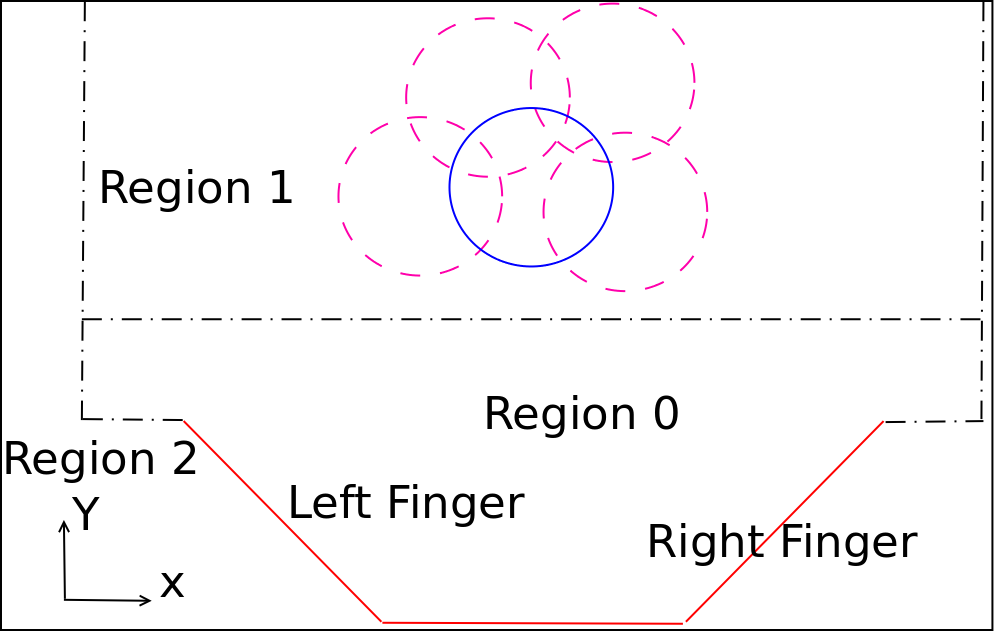
(b) Simplified model

Figure 3: Robot arm grasping task

TABLE II: Performance comparison on grasping cup

	Model Evaluation	V-REP simulation
States $|X|$	Continuous	Continuous
Actions $|A|$	7	7
Observations $|O|$	6	6
	Return Success Rate	Return Success Rate
POMCP	$14.17\pm 0.36$ $100\%$	$12.91\pm 2.10$ $94\%$
DESPOT	$11.35\pm 0.46$ $99.8\%$	$9.63\pm 2.52$ $92\%$
Mean MDP	$14.16\pm 0.46$ $98.6\%$	$11.28\pm 1.81$ $94\%$
POMDP-lite	$\mathbf{15.56\pm 0.31}$ $\mathbf{100\%}$	$\mathbf{15.46\pm 1.20}$ $\mathbf{98\%}$

VI Conclusion

We have introduced POMDP-lite, a subclass of POMDP with hidden variables that are either static or change deterministically. A POMDP-lite is equivalent to a set of MDPs indexed by a hidden parameter. By exploiting this equivalence, we have developed a simple online algorithm for POMDP-lite through model-based Bayesian reinforcement learning. Preliminary experiments suggest that the algorithm outperforms state-of-the-art general-purpose POMDP solvers on very large POMDP-lite models, makes it a promising tool for large-scale robot planning under uncertainty.

Currently, we are implementing and experimenting with the algorithm on a Kinova Mico robot for object manipulation. It is interesting and important to investigate extensions that handle large observation and action spaces.

Techinical Proofs

VI-A Proof of Lemma 1

Proof:

Let $\alpha_{0}$ denote $n(s,a)$, and let $\alpha_{i}$ denote $n(s,a,s_{i})$. According the definition of the Dirichlet distribution, $P(s_{j}|b,s,a)=\frac{\alpha_{j}}{\alpha_{0}}$. The reward bonus term can be described as

$$\frac{RB(b,s,a)}{\beta}=\underset{s_{j}\in S}{\sum}|P(s_{j}|b^{\prime},s,a)-P(s_{j}|b,s,a)|$$

$$=\underset{s_{k}}{\mathrm{E}}\bigg{[}\underset{s_{j}\neq s_{k}}{\sum}\big{(}\frac{\alpha_{j}}{\alpha_{0}}-\frac{\alpha_{j}}{\alpha_{0}+1}\big{)}+\big{(}\frac{\alpha_{k}+1}{\alpha_{0}+1}-\frac{\alpha_{k}}{\alpha_{0}}\big{)}\bigg{]}$$

$$=P(s_{k}|b,s,a)\bigg{(}\underset{s_{j}\neq s_{k}}{\sum}\frac{\alpha_{j}}{\alpha_{0}+\alpha_{0}^{2}}+\frac{\alpha_{0}-\alpha_{k}}{\alpha_{0}+\alpha_{0}^{2}}\bigg{)}$$

$$\leq\underset{s_{j}}{\sum}\frac{\alpha_{j}}{\alpha_{0}+\alpha_{0}^{2}}+\frac{\alpha_{0}}{\alpha_{0}+\alpha_{0}^{2}}=\frac{2}{1+\alpha_{0}}$$

As for the sample complexity, if $RB(b,s,a)<\kappa$, we have

$$RB(b,s,a)\leq\frac{2\beta}{1+\alpha_{0}}\leq\kappa\Rightarrow\alpha_{0}=O\big{(}\frac{\beta}{\kappa}\big{)}=O\big{(}\frac{|S|^{2}|A|}{\kappa(1-\gamma)^{2}}\big{)}$$

∎

VI-B Proof of Lemma 3

We first introduce some notations which will be used in the proof. Denote a $T$ step history as $h_{T}=\{b_{0},s_{0},a_{0},b_{1},s_{1},a_{1},...,b_{T},s_{T}\}$, where $b_{t}$ and $s_{t}$ is the belief and state at time step $t$. The following is a definition of $L_{1}$ divergence on reward function and transition function.

Definition 4

Denote $\mathbb{R}$ as the set of mean reward function, $\mathbb{T}$ as the set of mean transition function. i.e., given belief $b$, $\mathbb{R}(b)=\{R(b,s,a)|s\in S,a\in A\}$, $\mathbb{T}(b)=\{T(b,s,a,s^{\prime})|s,s^{\prime}\in S,a\in A\}$. Suppose the belief changes from $b_{i}$ to $b_{j}$, the $L_{1}$ divergence of $\mathbb{R}$ and $\mathbb{T}$ are denoted as:

$$\mathbb{R}(b_{i},b_{j})=\|\mathbb{R}(b_{j})-\mathbb{R}(b_{i})\|_{1}=\underset{s,a}{\sum}\big{|}R(b_{j},s,a)-R(b_{i},s,a)\big{|}$$

$$\mathbb{T}(b_{i},b_{j})=\|\mathbb{T}(b_{j})-\mathbb{T}(b_{i})\|_{1}$$

$$=\underset{s,a}{\sum}\underset{s^{\prime}}{\sum}\big{|}T(b_{j},s,a,s^{\prime})-T(b_{i},s,a,s^{\prime})\big{|}$$

Based on Definition 4, we introduce the regret of a $T$ step history if the belief is not updated each step.

Definition 5

Given a $T$ step history $h_{T}$, if the belief is not updated, the regret of the $i^{th}$ action is defined as $E(b_{0},i)=\mathbb{R}(b_{0},b_{i})+\frac{1}{1-\gamma}\mathbb{T}(b_{0},b_{i})$. Define $\mathcal{RE}(b_{0},T)=\underset{i=0}{\overset{T}{\sum}}\gamma^{i}E(b_{0},i,\pi)$ as the total regret of the history.

The following definition measures the extra value from reward bonus term when we are using internal reward.

Definition 6

Given a policy $T$ step history $h_{T}$, the reward bonus for the $i^{th}$ action is $B(b_{0},i)=RB(b_{0},s_{i},a_{i})$. Define $\mathcal{RB}(b_{0},T)=\underset{i=0}{\overset{T}{\sum}}\gamma^{i}B(b_{0},i)$ as the total extra value from reward bonus.

In the next lemma, we are going to bound the regret using the extra value from reward bonus.

Lemma 5

Given a $T$ step history $h_{T}$, let $\mathcal{RE}(b_{0},T)$ be the regret of not updating the belief, as defined in Definition 5. Let $\mathcal{RB}(b_{0},T)$ be the extra value from reward bonus term, as defined in Definition 6. If the constant tunning factor of reward bonus $\beta=O\big{(}\frac{|S|^{2}|A|T}{(1-\gamma)}\big{)}$, then $\mathcal{RB}(b_{0},T)\geq\mathcal{RE}(b_{0},T)$.

Proof:

We begin the proof by showing that the $L_{1}$ divergence of the reward function is bounded by the reward bonus if $\beta$ was chosen properly.

$$\mathbb{R}(b_{0},b_{i})=\underset{s,a}{\sum}\big{|}R(b_{i},s,a)-R(b_{0},s,a)\big{|}$$

$$=\underset{s,a}{\sum}\big{|}\underset{\theta_{i}\in\Theta}{\sum}R(\theta_{i},s,a)(b_{i}(\theta_{i})-b_{0}(\theta_{i}))\big{|}$$

$$\leq\underset{s,a}{\sum}\underset{\theta_{i}\in\Theta}{\sum}|b_{i}(\theta_{i})-b_{0}(\theta_{i})|$$

$$=|S||A|\|b_{i}-b_{0}\|_{1}\leq|S||A|\overset{i-1}{\underset{l=0}{\sum}}\|b_{l+1}-b_{l}\|_{1}$$

$$=\frac{|S||A|}{\beta}\overset{i-1}{\underset{l=0}{\sum}}RB(b_{l},s_{l},a_{l})$$

$$\leq\frac{|S||A|}{\beta}\overset{i-1}{\underset{l=0}{\sum}}RB(b_{0},s_{l},a_{l})$$

$$=\frac{|S||A|}{\beta}\overset{i-1}{\underset{l=0}{\sum}}B(b_{0},l)$$

The first inequality above follows from the fact that $R(\theta_{i},s,a)$ is bounded in $[0,1]$, and triangle inequality. The second inequality also follows from triangle inequality, i.e., $\|b_{s_{i}}-b_{0}\|_{1}\leq\|b_{s_{i}}-b_{s_{i-1}}\|_{1}+...+\|b_{s_{1}}-b_{0}\|_{1}$. The third inequality follows from our monotonicity assumption on the reward bonus: $RB(b_{l},s_{l},a_{l})\leq RB(b_{0},s_{l},a_{l})$.

Similarly, we can show that the $L_{1}$ divergence of the transition function is bounded by the reward bonus.

$$\mathbb{T}(b_{0},b_{s_{i}})\leq\frac{|S|^{2}|A|}{\beta}\overset{i-1}{\underset{l=0}{\sum}}B(b_{0},l)$$

Finally, we are going to show that the total regret $\mathcal{RE}(b_{0},T)$ of $h_{T}$ can be bounded by the extra value from reward bonus $\mathcal{RB}(b_{0},T)$:

$$\mathcal{RE}(b_{0},T)=\overset{T}{\underset{i=0}{\sum}}\gamma^{i}E(b_{0},i)$$

$$=\overset{T}{\underset{i=0}{\sum}}\gamma^{i}\bigg{(}\mathbb{R}(b_{0},b_{i})+\frac{1}{1-\gamma}\mathbb{T}(b_{0},b_{i})\bigg{)}$$

$$\leq O\bigg{(}\frac{|S|^{2}|A|}{\beta(1-\gamma)}\bigg{)}\overset{T}{\underset{i=0}{\sum}}\gamma^{i}\bigg{(}\overset{i-1}{\underset{l=0}{\sum}}B(b_{0},l)\bigg{)}$$

$$\leq O\bigg{(}\frac{|S|^{2}|A|T}{\beta(1-\gamma)}\bigg{)}\overset{T}{\underset{i=0}{\sum}}\gamma^{i}B(b_{0},i)=\mathcal{RB}(b_{0},i)$$

The first inequality above follows from the fact that the $L_{1}$ divergence of reward function and transition is bounded by the reward bonus for some value of $\beta$. The second inequality follows $\overset{T}{\underset{i=0}{\sum}}\gamma^{i}\bigg{(}\overset{i-1}{\underset{l=0}{\sum}}B(b_{0},l)\bigg{)}\leq\overset{T-1}{\underset{i=0}{\sum}}\gamma^{i}(T-i)B(b_{0},i)\leq T\overset{T}{\underset{i=0}{\sum}}\gamma^{i}B(b_{0},i)$.

∎

Now, we are ready to prove Lemma 3.

Proof:

Let $T=1/(1-\gamma)\ln(1/\epsilon(1-\gamma))$, then $|V^{*}(b_{0},s_{0},T)-V^{*}(b_{0},s_{0})|\leq\epsilon$ (see Lemma 2 of [9]), where $b_{0}$ and $s_{0}$ is the initial belief and state. Consider some state $s$, let $b_{t}$ be the new belief formed by updating $b_{0}$ after $t\leq T$ steps, then

$$\begin{split}&\mathcal{RB}(b_{0},t-1)-\mathcal{RE}(b_{0},t-1)+\\ &\tilde{V}^{*}_{T-t}(b_{0},s)-V^{*}_{T-t}(b_{t},s)\\ &=\mathcal{RB}(b_{0},t-1)-\mathcal{RE}(b_{0},t-1)+\\ &\underset{a}{\max}\bigg{\{}R(b_{0},s,a)+RB(b_{0},s,a)+\\ &\underset{s^{\prime}}{\sum}P(s^{\prime}|b_{0},s,a)\tilde{V}^{*}_{T-t-1}(b,s^{\prime})\bigg{\}}-\\ &\underset{a}{\max}\bigg{\{}R(b_{t},s,a)+\underset{s^{\prime}}{\sum}P(s^{\prime}|b_{t},s,a)\tilde{V}^{*}_{T-t-1}(b_{t+1},s^{\prime})\bigg{\}}\\ &\geq\mathcal{RB}(b_{0},t-1)-\mathcal{RE}(b_{0},t-1)+\\ &\underset{a}{\min}\bigg{\{}RB(b_{0},s,a)-\big{(}R(b_{t},s,a\big{)}-R(b_{0},s,a))+\\ &\underset{s^{\prime}}{\sum}P(s^{\prime}|b_{0},s,a)\tilde{V}^{*}_{T-t-1}(b_{0},s^{\prime})-\\ &\underset{s^{\prime}}{\sum}P(s^{\prime}|b_{t},s,a)\tilde{V}^{*}_{T-t-1}(b_{t+1},s^{\prime})\bigg{\}}\\ &\geq\mathcal{RB}(b_{0},t-1)-\mathcal{RE}(b_{0},t-1)+\\ &\underset{a}{\min}\bigg{\{}RB(b_{0},s,a)-\big{(}R(b_{t},s,a\big{)}-R(b_{0},s,a))-\\ &T\underset{s^{\prime}}{\sum}|P(s|b_{t},s,a)-P(s^{\prime}|b_{0},s,a)|+\\ &\underset{s^{\prime}}{\sum}P(s^{\prime}|b_{0},s,a)\big{(}\tilde{V}^{*}_{T-t-1}(b,s^{\prime})-\tilde{V}^{*}_{T-t-1}(b_{t+1},s^{\prime})\big{)}\bigg{\}}\\ &\geq\mathcal{RB}(b_{0},t)-\mathcal{RE}(b_{0},t)+\\ &\underset{a}{\min}\bigg{\{}\underset{s^{\prime}}{\sum}P(s^{\prime}|b_{0},s,a)\big{(}\tilde{V}^{*}_{T-t-1}(b,s^{\prime})-\tilde{V}^{*}_{T-t-1}(b_{t+1},s^{\prime})\bigg{\}}\\ &\geq\mathcal{RB}(b_{0},t)-\mathcal{RE}(b_{0},t)+\\ &\underset{s}{\min}\big{\{}\tilde{V}^{*}_{T-t-1}(b,s)-\tilde{V}^{*}_{T-t-1}(b_{t+1},s)\big{\}}\end{split}$$ (3)

The first inequality transformation in Equation 3 follows:

$$\underset{x}{\max}f(x)-\underset{x}{\max}g(x)\geq\underset{x}{\min}\big{(}f(x)-g(x)\big{)}$$

The second inequality transformation in Equation 3 follows:

$$\begin{split}&\underset{x}{\sum}p(x)f(x)-\underset{x}{\sum}q(x)g(x)\\ &\geq\underset{x}{\sum}p(x)(f(x)-g(x))-\underset{x}{\sum}|q(x)-p(x)|g(x)\end{split}$$

The third inequality transformation in Equation 3 follows the definition of $\mathcal{RB}$ and $\mathcal{RE}$.

Since $s$ is arbitrary in Equation 3, we have for any history $h_{T}$ and $t\leq T$,

$$\begin{split}&\mathcal{RB}(b_{0},t-1)-\mathcal{RE}(b_{0},t-1)+\\ &\tilde{V}^{*}_{T-t}(b_{0},s)-V^{*}_{T-t}(b_{t},s)\\ &\geq\mathcal{RB}(b_{0},t)-\mathcal{RE}(b_{0},t)+\\ &\underset{s}{\min}\big{\{}\tilde{V}^{*}_{T-t-1}(b,s)-\tilde{V}^{*}_{T-t-1}(b_{t+1},s)\big{\}}\end{split}$$ (4)

Where $\mathcal{RB}(b_{0},t)=0,\mathcal{RE}(b_{0},t)=0$ if $t\leq 0$.

Apply Equation 4 repeatedly for $T$ steps, we get

$$\tilde{V}^{*}_{T}(b_{0},s)-V^{*}_{T}(b_{0},s)$$

$$\geq\mathcal{RB}(b_{0},T)-\mathcal{RE}(b_{0},T)+$$

$$\underset{s}{\min}\big{\{}\tilde{V}^{*}_{T-T}(b,s)-\tilde{V}^{*}_{T-T}(b_{T+1},s)\big{\}}\geq 0$$

The second inequality above follows Lemma 5 then we have $\tilde{V}^{*}(b_{0},s)\geq\tilde{V}^{*}_{T}(b_{0},s)\geq V^{*}_{T}(b_{0},s)\geq V^{*}(b_{0},s)-\epsilon$, which proves our lemma.

∎

VI-C Proof of Lemma 4

Proof:

Consider the sequence of states, actions by following $\pi_{t}$ at state $s_{t}$ and belief $b_{t}$, $p_{t}=s_{t},a_{t},s_{t}^{1},a_{t}^{1},...,s_{t}^{m},a_{t}^{m}$. Suppose $(s_{t}^{k},a_{t}^{k})$ is the first state action pair not in $K$ is generated. We have $\tilde{V}^{\pi}(b_{t},s_{t})=\overset{k-1}{\underset{i=0}{\sum}}\gamma^{i}\tilde{R}(b_{t},s_{t}^{i},a_{t}^{i})+\gamma^{k}\tilde{Q}(b_{t},s_{t}^{k},a_{t}^{k})$ and $V_{M_{K_{t}}}^{\pi}(b_{t},s_{t})=\overset{k-1}{\underset{i=0}{\sum}}\gamma^{i}R(b_{t},s_{t}^{i},a_{t}^{i})+\gamma^{k}\tilde{Q}(b_{t},s_{t}^{k},a_{t}^{k})$. Then, $\tilde{V}^{\pi}(b_{t},s_{t})-V_{M_{K_{t}}}^{\pi}(b_{t},s_{t})\leq\overset{k-1}{\underset{i=0}{\sum}}\gamma^{i}\epsilon(1-\gamma)\leq\epsilon$. ∎

References

- [1] J. Asmuth, L. Li, M. L. Littman, A. Nouri, and D. Wingate, “A bayesian sampling approach to exploration in reinforcement learning,” in Proceedings of the Twenty-Fifth Conference on Uncertainty in Artificial Intelligence, 2009.
- [2] H. Bai, S. Cai, D. Hsu, and W. Lee, “Intention-aware online POMDP planning for autonomous driving in a crowd,” in Proc. IEEE Int. Conf. on Robotics & Automation, 2015.
- [3] H. Bai, D. Hsu, and W. Lee, “Planning how to learn,” in Proc. IEEE Int. Conf. on Robotics & Automation, 2013.
- [4] T. Bandyopadhyay, K. Won, E. Frazzoli, D. Hsu, W. Lee, and D. Rus, “Intention-aware motion planning,” in Algorithmic Foundations of Robotics X—Proc. Int. Workshop on the Algorithmic Foundations of Robotics (WAFR), 2012.
- [5] F. Doshi-Velez and G. Konidaris, “Hidden parameter Markov decision processes: A semiparametric regression approach for discovering latent task parametrizations,” arXiv preprint arXiv:1308.3513, 2013.
- [6] A. Fern, S. Natarajan, K. Judah, and P. Tadepalli, “A decision-theoretic model of assistance,” in Proc. AAAI Conf. on Artificial Intelligence, 2007.
- [7] K. Hsiao, L. Kaelbling, and T. Lozano-Pérez, “Grasping POMDPs,” in Proc. IEEE Int. Conf. on Robotics & Automation, 2007.
- [8] L. Kaelbling, M. Littman, and A. Cassandra, “Planning and acting in partially observable stochastic domains,” Artificial Intelligence, vol. 101, no. 1–2, pp. 99–134, 1998.
- [9] M. Kearns and S. Singh, “Near-optimal reinforcement learning in polynomial time,” Machine Learning, vol. 49, no. 2-3, pp. 209–232, 2002.
- [10] L. Kocsis and C. Szepesvári, “Bandit based monte-carlo planning,” in Machine Learning: ECML 2006. Springer, 2006, pp. 282–293.
- [11] J. Z. Kolter and A. Y. Ng, “Near-bayesian exploration in polynomial time,” in Proceedings of the 26th Annual International Conference on Machine Learning, 2009.
- [12] M. Koval, N. Pollard, and S. Srinivasa, “Pre- and post-contact policy decomposition for planar contact manipulation under uncertainty,” Int. J. Robotics Research, 2015.
- [13] H. Kurniawati, D. Hsu, and W. Lee, “SARSOP: Efficient point-based POMDP planning by approximating optimally reachable belief spaces,” in Proc. Robotics: Science & Systems, 2008.
- [14] S. Nikolaidis, R. Ramakrishnan, K. Gu, and J. Shah, “Efficient model learning from joint-action demonstrations for human-robot collaborative tasks,” in Proc. ACM/IEEE Int. Conf. on Human-Robot Interaction, 2015.
- [15] S. C. Ong, S. W. Png, D. Hsu, and W. S. Lee, “Planning under uncertainty for robotic tasks with mixed observability,” The International Journal of Robotics Research, vol. 29, no. 8, pp. 1053–1068, 2010.
- [16] C. H. Papadimitriou and J. N. Tsitsiklis, “The complexity of markov decision processes,” Mathematics of operations research, vol. 12, no. 3, pp. 441–450, 1987.
- [17] P. Poupart, N. Vlassis, J. Hoey, and K. Regan, “An analytic solution to discrete bayesian reinforcement learning,” in Proceedings of the 23rd international conference on Machine learning. ACM, 2006.
- [18] E. Rohmer, S. P. Singh, and M. Freese, “V-rep: A versatile and scalable robot simulation framework,” in Intelligent Robots and Systems (IROS), 2013 IEEE/RSJ International Conference on. IEEE, 2013, pp. 1321–1326.
- [19] S. Ross, J. Pineau, S. Paquet, and B. Chaib-Draa, “Online planning algorithms for POMDPs,” J. Artificial Intelligence Research, vol. 32, no. 1, pp. 663–704, 2008.
- [20] N. Roy and S. Thrun, “Coastal navigation with mobile robots,” in Advances in Neural Information Processing Systems. The MIT Press, 1999, vol. 12, pp. 1043–1049.
- [21] K. Seiler, H. Kurniawati, and S. Singh, “An online and approximate solver for pomdps with continuous action space,” in Proc. IEEE Int. Conf. on Robotics & Automation, 2015.
- [22] D. Silver and J. Veness, “Monte-Carlo planning in large POMDPs,” in Advances in Neural Information Processing Systems, 2010.
- [23] T. Smith and R. Simmons, “Point-based POMDP algorithms: Improved analysis and implementation,” in Proc. Conf. on Uncertainty in Artificial Intelligence, 2005.
- [24] A. Somani, N. Ye, D. Hsu, and W. Lee, “DESPOT: Online POMDP planning with regularization,” in Advances in Neural Information Processing Systems, 2013.
- [25] E. Sondik, “The optimal control of partially observable Markov processes,” Ph.D. dissertation, Stanford University, Stanford, California, USA, 1971.
- [26] J. Sorg, S. P. Singh, and R. L. Lewis, “Variance-based rewards for approximate bayesian reinforcement learning,” in UAI, Proceedings of the Twenty-Sixth Conference on Uncertainty in Artificial Intelligence, 2010.
- [27] A. L. Strehl, L. Li, and M. L. Littman, “Incremental model-based learners with formal learning-time guarantees,” in UAI, Proceedings of the 22nd Conference in Uncertainty in Artificial Intelligence, 2006.
- [28] S. Thrun, W. Burgard, and D. Fox, Probabilistic Robotics. The MIT Press, 2005.