Damping and power spectra of quasi-periodic intensity disturbances above a solar polar coronal hole^∗

Abstract

We study intensity disturbances above a solar polar coronal hole seen in the AIA 171 Å and 193 Å passbands, aiming to provide more insights into their physical nature. The damping and power spectra of the intensity disturbances with frequencies from 0.07 mHz to 10.5 mHz are investigated. The damping of the intensity disturbances tends to be stronger at lower frequencies, and their damping behavior below 980${}^{{}^{\prime\prime}}$(for comparison, the limb is at 945${}^{{}^{\prime\prime}}$) is different from what happens above. No significant difference is found between the damping of the intensity disturbances in the AIA 171 Å and that in the AIA 193 Å. The indices of the power spectra of the intensity disturbances are found to be slightly smaller in the AIA 171 Å than in the AIA 193 Å, but the difference is within one sigma deviation. An additional enhanced component is present in the power spectra in a period range of 8–40 minutes at lower heights. While the power spectra of spicule is highly correlated with its associated intensity disturbance, it suggests that the power spectra of the intensity disturbances might be a mixture of spicules and wave activities. We suggest that each intensity disturbance in the polar coronal hole is possibly a series of independent slow magnetoacoustic waves triggered by spicular activities.

1 Introduction

Intensity disturbances in solar polar coronal holes have been discovered since Withbroe (1983), who reported a 10% variation in the Mg x 625 Å line radiance in polar plumes. The intensity disturbances tend to have a periodicity of 5–30 minutes (e.g. Withbroe 1983; Ofman et al. 1997; DeForest & Gurman 1998), and propagate with a speed of 50–200  km s^-1 (e.g. DeForest & Gurman 1998; Banerjee et al. 2009; Krishna Prasad et al. 2011; Jiao et al. 2015, among others).

Intensity disturbances are usually interpreted in terms of slow magnetoacoustic waves given that they propagate at roughly the sound speed (Ofman et al. 1999). Banerjee et al. (2009) found that the propagating speeds of the intensity disturbances increase from 75  km s^-1 at 0.6 MK (Ne viii) to 125  km s^-1 at 1.3 MK (Fe xii), which is expected given the temperature dependence of sound speeds in the slow wave scenario. Spectroscopic study using SUMER observations lent further support to this scenario (Gupta et al. 2012). The multi-passband data from SDO/AIA revealed that the propagation speed of intensity disturbances varies in different passpands  (Krishna Prasad et al. 2011). Furthermore, the amplitude and damping length are smaller in hotter channels (Krishna Prasad et al. 2011, 2012). In the slow wave scenario, this temperature-dependence can be readily accounted for if electron heat conduction is the primary mechanism for the damping. Recently, by analysing data from AIA 171 Å, 193 Å and 211 Å passbands, Su et al. (2014) discovered that the amplitude of intensity disturbances increases with height in the lower corona (0–9 Mm above the solar limb). They found that the acoustic velocities inferred from the scale height highly correlate with the phase speeds of the intensity disturbances, and therefore concluded that the intensity disturbances in the lower corona are likely slow magnetoacoustic waves. Furthermore, Su (2014) statistically measured the phase speeds of intensity disturbances in polar regions observed by AIA 171 Å, 193 Å and 211 Å, and found that the speed ratios in different channels are consistent with the theoretical expectations for acoustic waves. By testing a 2.5D magnetohydrodynamic simulation to a flare loop, Fang et al. (2015) confirmed that the intensity disturbances following to chromospheric evaporation in the flare loop is slow mode waves.

An alternative interpretation for intensity disturbances is that they are quasi-periodic upflows, as was first suggested by McIntosh et al. (2010). Using STEREO observations, McIntosh et al. (2010) found that high speed jets tend to occur quasi-periodically with a periodicity of 5–25 minutes, and travel along polar plumes with a speed of 135  km s^-1 and an apparent brightness enhancement of $\sim 5\%$. A dedicated spectroscopic study using Hinode/EIS time-series observations revealed that repetitive high-velocity upflows, present as faint excess emission at $\sim$100  km s^-1 in blue wing of coronal lines, are correlated to the intensity disturbances in the corona (Tian et al. 2011).

It is difficult to distinguish waves and flows in observations (De Moortel et al. 2015) and it is not easy to separate different modes of waves since they can appear together in the same features (Zhang et al. 2015). However, the wave and flow scenarios are not necessarily mutually exclusive. Numerical studies by Ofman et al. (2012) and Wang et al. (2013) have shown that any upflow pulse at the coronal base results in propagating intensity disturbances guided by open flux tubes. An observational evidence supporting this understanding was offered by Jiao et al. (2015), where they provided convincing evidence that spicular activities in the solar transition region are one of the important sources triggering intensity disturbances in the corona. The connection between intensity disturbances in the corona and spicular activities in the lower atmosphere was recently confirmed by Samanta et al. (2015).

While propagating, slow magnetoacoustic waves are expected to be dissipated by such mechanisms as compressive viscosity (Ofman et al. 2000), electron thermal conduction (De Moortel & Hood 2003) and mode coupling (De Moortel et al. 2004). They may also dissipate by developing into shocks (Verwichte et al. 2008), given their amplitude growth in the presence of gravitational stratification (De Moortel & Hood 2004). Hence, investigations into the damping of intensity disturbances can help understand whether the intensity disturbances are slow magnetoacoustic waves. By analyzing observations from SDO/AIA, Krishna Prasad et al. (2014) obtained the frequency-dependence of the damping length of the intensity disturbances observed in a polar coronal hole, and found that the damping length tends to increase rather than decreasing with frequency. This discovery seems to be inconsistent with linear wave theory. However, the same analysis in on-disk plume-like structures (Krishna Prasad et al. 2014) shows the opposite behaviour. Gupta (2014) also studied intensity disturbances in a solar polar coronal hole observed by the AIA 171 Å channel, and found that low-frequency waves propagate further compared to high-frequency waves. Within a plume structure, he also found that the damping of intensity disturbances in the polar coronal hole follows two distinct profiles at two different height ranges (between 0–10 Mm and 10–70 Mm).

A power spectrum describes the power distribution in the frequency space. It can be used to reveal whether any frequency is preferred in a broadband spectrum. Studies of power spectrum are helpful to tell what happens in the solar atmosphere (Ireland et al. 2015). In a polar coronal hole observed by the AIA 171 Å channel, Gupta (2014) deduced power spectra of intensity disturbances at six individual points. The spectra were found to follow Kolmogorov’s law (power index$=$5/3), suggesting a possible connection between intensity disturbances and turbulence.

In this work, we examine intensity disturbances above a solar polar coronal hole in substantial detail, aiming to shed more light on the physical nature of intensity disturbances. To this end, we examine the damping and power spectra of intensity disturbances as identified in two different AIA channels. In the following, we describe the observations and methods of data analysis in Section 2, present our results and discussion in Section 3, and give a summary in Section 4.

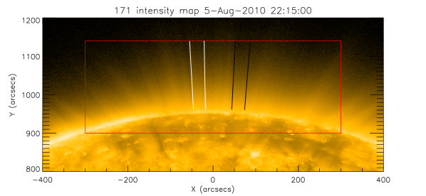
Figure 1: The studied polar coronal hole region (outlined by red lines) seen in AIA 171 Å. The region between two white lines outline a region filled by plumes. The region between two black lines mark the inter-plume region that is relative dark. The intensity is shown on a log scale.

2 Observations and data analysis

The data used in this study were obtained from 21:50 UT, 5 August 2010 to 01:50 UT, 6 August 2010 by AIA (Lemen et al. 2012), with a spatial resolution of 1.2${}^{{}^{\prime\prime}}$and a cadence of 12 s. We aim to investigate intensity disturbances in the north polar region with solar X between $-$300${}^{{}^{\prime\prime}}$and 300${}^{{}^{\prime\prime}}$ where a coronal hole is clearly seen (Figure 1). The solar limb at X=0 is located at Y=945${}^{{}^{\prime\prime}}$. Since intensity disturbances are a coronal phenomenon, we investigate the damping and power spectra of intensity disturbances observed by the two channels at coronal temperatures, namely 171 Å with response function peaking at 0.8 MK and 193 Å with response function peaking at 1.2 MK. The fast Fourier transform (FFT) routine in the IDL library was used to extract the evolution of coronal features in the frequency space.

Figure 1 presents the three regions that we analyze: the entire coronal hole (the red box, 301 pixels at any given height above the limb), a plume region bordered by the white lines (18 pixels at any given height above the limb), and an inter-plume region sandwiched between the black lines (19 pixels at any given height above the limb) in Fig. 1. Averaging the signals from the entire coronal hole substantially enhances the signal-to-noise ratio, thereby enabling one to examine the overall behavior of the intensity disturbances in this region. On the other hand, distinguishing between a plume and an inter-plume region allows one to tell whether the physical properties of the intensity disturbances depend on the magnetic environment.

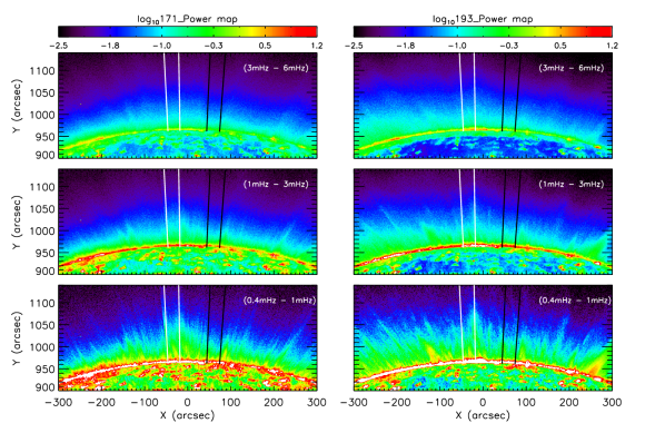
Figure 2: Power map of the polar coronal hole at 3–6 mHz (top), 1–3 mHz (middle) and 0.4–1 mHz (bottom). The left (right) column displays the power map deduced from the AIA 171 Å (193 Å) emissions. The plume and inter-plume regions are denoted by the white and black lines, respectively. Here the Fourier power is shown on a log scale.

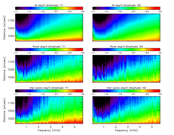
Figure 3: The variation of normalised amplitude along the solar radial direction above the limb averaging from three different regions (top row: the whole coronal hole, middle row: plume region, bottom row: inter-plume region, see Section 2 and Fig. 1 for details of the locations of these regions). The shown amplitude at any particular frequency is normalised by that at the same frequency at the radius of 965${}^{{}^{\prime\prime}}$. The intensity disturbances in AIA 171 Å (left column) and 193 Å (right column) are displayed.

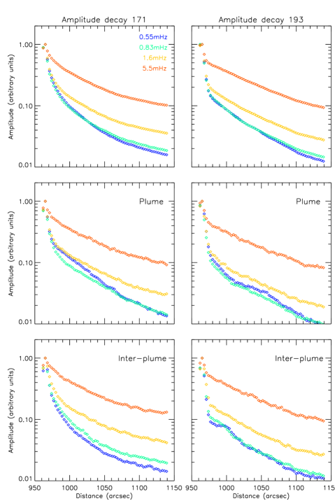
Figure 4: Damping of the intensity disturbances in the polar coronal hole. The results from the AIA 171 Å emission are shown in the left column and the 193 Å in the right column. Top row: coronal hole average, middle row: plume region and bottom row: inter-plume region.

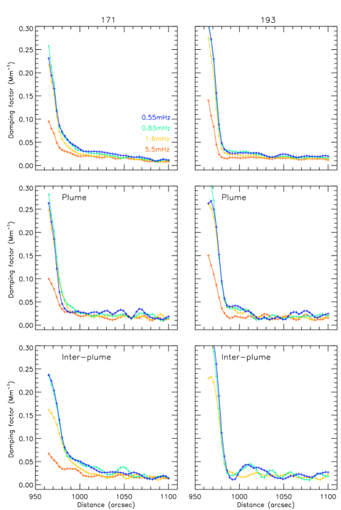
Figure 5: Local damping factor deduced from the log-normal plots shown in Fig. 4.

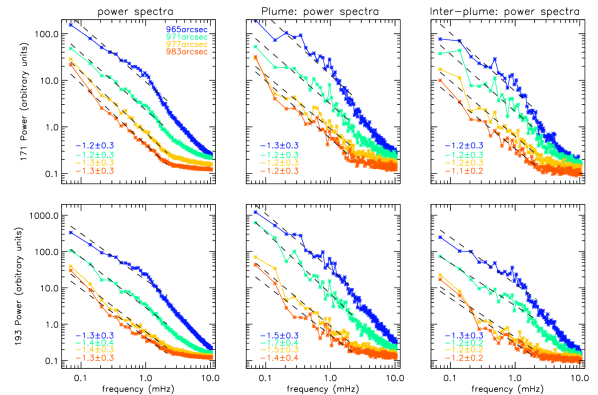
Figure 6: Power spectra of the intensity disturbances in the polar coronal hole. The spectra are obtained from four different heights (blue: 965${}^{{}^{\prime\prime}}$, green: 971${}^{{}^{\prime\prime}}$, orange: 977${}^{{}^{\prime\prime}}$, red: 983${}^{{}^{\prime\prime}}$). The left row is the spectra from AIA 171 Å and the bottom one is from AIA 193 Å. The spectra in the left column are from coronal hole average, the middle column are from plume region and the right column are from inter-plume region. The over-plotted dashed lines are fittings to the power-law spectra in the form $P(f)\propto f^{\alpha}$. The errors of the power indices $\alpha$ are also given (see details in the main text)

.

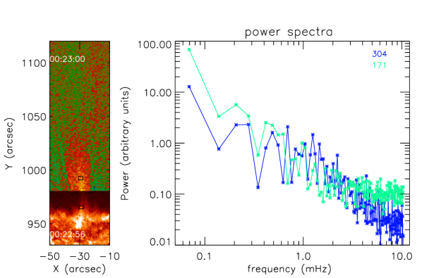
Figure 7: Power spectra (right panel) of a spicule seen in AIA 304 Å (blue) and its associated intensity disturbance seen in AIA 171 Å (green). The regions to calculate the power spectra are shown in the left panel marked as black boxes, where the top one in the intensity disturbance seen in AIA 171 Å and the bottom one in the associated spicule seen in AIA 304 Å.

3 Results

Fig. 2 shows the power distribution in the polar coronal hole region in the frequency ranges 3–6 mHz (the top row), 1–3 mHz (middle) and 0.4–1 mHz (bottom) seen in the AIA 171 Å (the left column) and 193 Å(right). At low frequencies (0.4–1 mHz), the power images in both AIA 171 Å and 193 Å above the limb show many distinguishable radial structures filling the whole region. Such radial structures are so-called intensity disturbances. At higher frequencies, the intensity disturbances are mixed with each other and thus individual intensity disturbances are difficult to distinguish (see the top and middle panels in Fig. 1). Comparing the left and right columns, one sees that the intensity disturbances as seen in AIA 171 Å are similar to those in AIA193 Å. In line with Krishna Prasad et al. (2012) and Gupta (2014), the power of the intensity disturbances decreases with altitude, suggesting that intensity disturbances are spatially damped. In the next section, we provide a detailed examination on this damping together with its dependence on frequency and temperature.

3.1 Damping of the intensity disturbances

Figure 3 shows the amplitude distribution as a function of frequency and distance. Because the intensity disturbances at a given height are much stronger at lower than at higher frequencies (see Fig. 2), the normalized Fourier amplitude is shown in Fig. 3 rather than the original value. In practice, at any given frequency, the Fourier amplitude at an arbitrary height is normalized by the corresponding value at 965${}^{{}^{\prime\prime}}$. The first impression from Fig. 3 is that the overall behavior of the amplitude distribution is similar in the three examined regions. In particular, the distribution is similar for the plume and inter-plume regions, suggesting that the differences in the physical parameters therein do not qualitatively change the dependence of the Fourier amplitude on height and frequency. Furthermore, the spatial damping does not show a monotonic frequency dependence. It clearly shows that this damping tends to increase with frequency first in lower frequencies and then decrease in higher frequencies. This dependency is clearly seen in the results of the entire coronal hole (top row in Fig. 3) where the frequency-dependence changes its behavior around 0.7 mHz. A similar dependency of the damping in plume and inter-plume regions can also be seen, although not very clear.

The frequency dependence of the spatial damping of intensity disturbances is further examined in Fig. 4, where the spatial profiles of the normalized Fourier amplitude at a number of different frequencies are displayed as labeled. One sees that regardless of the region examined, the spatial damping of intensity disturbances tends to be stronger at lower frequencies. However, it turns out that deducing a damping length is not straightforward, since the spatial profiles at the chosen frequencies do not possess an exponential height dependence (note that a globally exponential behavior would yield a straight line given that the amplitude is plotted on a log scale). Nevertheless, it is possible to deduce a local damping factor based on a linear fit to a few (5 in this study) data points centering at a given height by assuming that the amplitude follows an exponential damping law locally. The damping factor is given by the local slope obtained from the linear fit operated as above. The damping factor quantifies how fast the amplitude of a disturbance decreases when it propagates in the solar atmosphere.

Figure 5 presents the height variation of the damping factor for the same set of frequencies. The damping profiles seems to be close to Gaussian below 980${}^{{}^{\prime\prime}}$, and then the damping factor nearly settles to a constant beyond 980${}^{{}^{\prime\prime}}$, suggesting that the spatial damping becomes an exponential one. However, the damping factor below 980${}^{{}^{\prime\prime}}$ shows some considerable height dependence. This indicates that the mechanisms for spatially damping the intensity disturbances below 980${}^{{}^{\prime\prime}}$are different from those beyond. Despite this complication, the damping factor at a given height tends to decrease with frequency. Note that the two-step spatial damping and the inverse correlation between frequency and the damping factor were also noticed by Gupta (2014, their Figs. 7&8). These two features, the frequency dependence of damping factor in particular, seem difficult to understand if intensity disturbances are a continuous spectrum of slow waves emitted by, e.g., a broadband source at some fixed location. The reason is that, with the sound speed given, the wavelength becomes shorter with increasing frequency and consequently slow waves are expected to experience stronger damping, provided that ion viscosity or electron heat conduction are the primary damping mechanisms (see also Krishna Prasad et al. 2014).

3.2 Power spectra of the intensity disturbances

More insights can be gained by examining Fig. 6, where the power spectra of the intensity disturbances at a number of heights are shown for the three examined regions imaged in both 171 Å and 193 Å channels. The power spectra at a given height in a region are obtained from averaging the whole area of the region parallel to the limb (see Section 2) and 9 pixels around the given height. Fittings are given for a power spectrum of each pixel in each region at a given height and a given observing passband to reveal the power-law behavior of the spectra. The average and standard deviation ($\sigma$) of the power-law indices at a given height and a given passband are given in Fig. 6. Comparing different passbands, one can see that the power-law index ($\alpha$) is slightly larger in magnitude in the hotter channel (AIA 193 Å). However, the difference is small and cannot be distinguished within one sigma deviation. While comparing different regions, we found the power-law indices are larger in magnitude in AIA 193 Å plume region. One can also see that the power-laws provide a rather satisfactory description for the power spectra until a knee is reached at $\sim 2-3$ mHz, beyond which the spectra flattens. At the lowest height examined (965${}^{{}^{\prime\prime}}$), in all three regions, some excess power is present in the frequencies ranging from 0.4 mHz to 2 mHz (i.e. 8–40 minutes in period). As was discussed in Ireland et al. (2015), this excess power may derive from upward propagating disturbances generated in the lower parts of the solar atmosphere. What is new in Fig. 6 is that the spectra slope beyond the spectral knee tends to decrease in magnitude with height. This is also at variance with the interpretation that intensity disturbances are propagating slow waves generated by a continuous broadband driver. The reason is, the mechanisms dominating the spatial dependence of the Fourier amplitudes either are frequency-insensitive (gravitational stratification and magnetic field divergence) or provide a damping efficiency that correlates positively with frequency (ion viscosity and electron heat conduction) (Krishna Prasad et al. 2014).

Given a power-law-like behavior both below and beyond the spectral knee, one may speculate that turbulence may be at work that transfers energy from lower to higher frequencies, thereby replenishing the power at higher frequencies and consequently increasing the effective damping length. However, this is unlikely the case for the following two reasons. First, most of the obtained spectral slopes, except the ones obtained in the plume region observed by the AIA 193 Å, range from $-1.1$ to $-1.4$ (the uncertainties of these indices are rather substantial though). These nominal values agree with neither the value expected in a low-$\beta$ environment for isotropic hydrodynamic turbulence ($-5/3$) nor the ones expected for isotropic ($-3/2$) or anisotropic ($-2$ for the parallel wavenumber spectra) MHD turbulence (Cho et al. 2003). Second, if the spectral transfer is due to nonlinear interactions among slow waves, the efficiency of this transfer is expected to be at most proportional to the square of the amplitude of the waves at low frequencies. However, the amplitude of the intensity disturbances summed over all frequencies amount to only a few percent of the background intensity, let alone the amplitude in a particular frequency range. The consequent nonlinear interaction is therefore expected to be rather inefficient.

So now how to understand the frequency-dependent spatial damping of the intensity disturbances in view of their frequency spectra? Our tentative interpretation is that, rather than comprising a continuous spectrum of slow waves, these spectra may reflect a series of intermittent slow waves where adjacent slow wave pulses are rather randomly separated in response to the activities that excite these pulses. What this means is that not all frequency components in a spectrum can be attributed to waves, and consequently, the spatial damping of individual components at various frequencies does not necessarily need to be contrasted with the theoretical expectations of slow wave damping. For illustration purposes, consider the toy model where some activity repeats, say, every 10 minutes in the transition region or chromosphere. Each instance of this activity generates a velocity pulse that impinges on the corona, leading to the eventual development of a slow wave pulse (e.g., Wang et al. 2013). Now that slow waves are dispersion-less, the intensity time series at some coronal height will consist of a series of wave pulses with a temporal spacing of 10 minutes. This 10-minute periodicity will make it into the frequency spectrum when the time series is Fourier-analyzed. However, it does not correspond to any wave signal, and the spatial variation of the spectral component in a frequency range around this periodicity does not need to agree or disagree with wave theory. In reality, the temporal spacing between two instances of activities lower down should be much more irregular than being uniform. The corresponding spectral components, which themselves do not correspond to waves, are expected to appear in the frequency spectra of the intensity disturbances as well.

Figure 7 provides an observational test of the above-mentioned picture, where the frequency spectrum of the repetitive spicular activities measured by AIA304 Å is compared with that of the intensity disturbances in the corona (AIA 171 Å). As recently found by Jiao et al. (2015) and Samanta et al. (2015), spicular activities are an important source for generating coronal intensity disturbances. One finds from Fig. 7 that the two spectra are indeed well correlated, lending support to the notion that the frequency components in the exciters (spicular activities in the present case) can contribute to the spectra of coronal intensity disturbances.

4 Summary

We have examined the damping and power spectra of the intensity disturbances in a polar coronal hole. The damping of the intensity disturbances at low frequencies is stronger than that at higher frequencies. The damping of the intensity disturbances becomes exponential only above 980${}^{{}^{\prime\prime}}$, suggesting that the intensity disturbances may experience a two-step damping rather than being damping by a single mechanism operating at all heights. We found that the power spectra of the intensity disturbances show power-laws with roughly the same index in different regions in a chosen AIA passband. While comparing different passbands, one can see that the power-law index of the power spectra is slightly larger in magnitude in the hotter channel (AIA 193 Å). However, the difference is small and cannot be distinguished within one sigma deviation. Comparing different regions, we found it is larger in magnitude in AIA 193 Å plume region. An additional enhanced component is present in the power spectra in a period range of 8–40 minutes at lower heights, which suggests a possible contribution of upward propagating waves from lower parts of the solar atmosphere. The observed damping and power spectra of the intensity disturbances are found to be at variance with the interpretation that coronal intensity disturbances are a continuous spectrum of slow waves excited by broadband drivers. Instead, coronal intensity disturbances may consist of randomly separated slow wave pulses with a substantial number of their frequency components bearing signatures of the exciters. One important exciter is attributed to spicular activities as seen in the AIA 304 Å channel.