Fluid Stretching as a Lévy Process

Abstract

We study the relation between flow structure and fluid deformation in steady two-dimensional random flows. Beyond the linear (shear flow) and exponential (chaotic flow) elongation paradigms, we find a broad spectrum of stretching behaviors, ranging from sub- to superlinear, which are dominated by intermittent shear events. We analyze these behaviors from first principles, which uncovers stretching as a result of the non-linear coupling between Lagrangian shear deformation and velocity fluctuations along streamlines. We derive explicit expressions for Lagrangian deformation and demonstrate that stretching obeys a coupled continous time random walk, which for broad distributions of flow velocities describes a Lévy walk for elongation. The derived model provides a direct link between the flow and deformation statistics, and a natural way to quantify the impact of intermittent shear events on the stretching behavior, which can have strong anomalous diffusive character.

The deformation dynamics and stretching history of material fluid elements are fundamental for the understanding of hydrodynamic phenomena ranging from scalar dispersion, pair dispersion Shlesinger et al. (1987); Rast and Pinton (2011); Thalabard et al. (2014), mixing Kleinfelter et al. (2005); Villermaux and Duplat (2006); Jha et al. (2011); De Barros et al. (2012); Le Borgne et al. (2015); Ye et al. (2015) and reaction Ranz (1979); Tartakovsky et al. (2008); Engdahl et al. (2014); Hidalgo et al. (2015) to the alignment of material elements Lapeyre et al. (1999) and the distribution of stress in complex fluids Truesdell and Noll (1992). Fluid elements constitute the Lagrangian support of a transported scalar. Thus, their deformation histories determine the organization of the scalar distribution into lamellar structures Kalda (2000); Villermaux and Duplat (2003); Villermaux (2012); Le Borgne et al. (2013). Observed broad scalar concentration distributions are a manifestation of a broad distribution of stretching and compression rates and can explain intermittent patterns of scalar increment distributions Kalda (2000); Villermaux and Duplat (2003). The temporal scaling of the average elongation $\langle\ell(t)\rangle$ of material lines controls the decay of scalar variance, the effective kinetics of chemical reactions and the distribution of scalar gradients Ottino (1989). The mechanisms of linear stretching due to persistent shear deformation, and exponential stretching in chaotic flows have been well understood Ottino (1989). Observations of sub-exponential and non-linear fluid elongation of material element deformation in isotropic flows et al. (2000); Duplat et al. (2010); Le Borgne et al. (2013), pair-dispersion Shlesinger et al. (1987); Goto and Vassilicos (2004); Rast and Pinton (2011); Thalabard et al. (2014); Afik and Steinberg (2015), and scalar variance decay Nelkin and Kerr (1981); Vassilicos (2002), however, challenge these paradigms and ask for new dynamic frameworks. Even if stretching may be expected to be asymptotically exponential, there generally exists a persistent pre-asymptotic algebraic mixing regime  Vassilicos (2002), which is critical as most mixing and associated chemical reactions are likely to occur at early times.

While exponential stretching regimes are well understood, the theoretical description of algebraic stretching and mixing behaviors is still debated and different mechanisms have been proposed to describe it, including fractal/spiral mixing (e.g. Vassilicos, 2002), non-sequential stretching (e.g. Duplat et al., 2010), and modified Richardson laws (e.g. Nelkin and Kerr, 1981). The dynamics of particle pair separation, for example, have been described using Levy processes and continuous time random walks Shlesinger et al. (1987); Bofetta and Sokolov (2002); Thalabard et al. (2014). Elongation time series for stretching in $d=2$ dimensional heterogeneous porous media flows have been modeled as geometric Brownian motions Le Borgne et al. (2015).

Most stochastic stretching models, however, do not provide relations between the deformation dynamics and the local Lagrangian and Eulerian deformations and flow structure. This means, the fluctuation mechanisms that cause observed algebraic stretching are often not known. Broad velocity distributions as observed in disordered media Bouchaud and Georges (1990) and porous media flows Le Borgne et al. (2008a); Bijeljic et al. (2011) lead to anomalous dispersion, which has been the subject of intense theoretical and experimental studies Bouchaud and Georges (1990); Berkowitz and Scher (1997); Seymour et al. (2004); Bijeljic et al. (2011); De Anna et al. (2013). The consequences for fluid stretching are much less known. Thus, we focus here on the relation between velocity fluctuations and fluid deformation in non-helical steady random flows, such as steady $d=2$ dimensional pore-scale and $d=2$ and $d=3$ dimensional Darcy-scale flows in heterogeneous media Sposito (1994); Lester et al. (2016). Such flows occur in natural and engineered materials including porous and fractured rocks Bear (1972), porous films, carbon layers, chromatography, packed bed reactors Brenner and Edwards (1993); Jakobsen (2008), biofilms and biological tissue Vafai (2010). We derive a mechanism that leads to a broad range of sub-exponential and power-law stretching behaviors. We formulate Lagrangian deformation in streamline coordinates Winter (1982), which relates elongation to Lagrangian velocities and shear deformation. The consequences of this coupling are studied in the framework of a continuous time random walk (CTRW) Montroll and Weiss (1965); Scher and Lax (1973); Zaburdaev et al. (2015) that links transit times of material fluid elements to elongation through Lagrangian velocities. We show that non-linear stretching behaviors can be caused by broad velocity distributions.

Our analysis starts with the equation of motion of a fluid particle in a steady spatially varying flow field. The particle position ${\mathbf{x}}(t|{\mathbf{a}})$ in the divergence-free flow field ${\mathbf{u}}({\mathbf{x}})$ evolves according to the advection equation

$$\frac{d{\mathbf{x}}(t|{\mathbf{a}})}{dt}={\mathbf{v}}(t),$$ (1)

where ${\mathbf{v}}(t)={\mathbf{u}}[{\mathbf{x}}(t|{\mathbf{a}})]$ denotes the Lagrangian velocity. The initial condition is given by ${\mathbf{x}}(t=0|{\mathbf{a}})={\mathbf{a}}$. The particle movement along a streamline can be formulated as

$$\frac{ds(t)}{dt}=v(t), dt=\frac{ds}{v_{s}(s)},$$ (2)

where $s(t)$ is the distance travelled along the streamline, $v(t)=|{\mathbf{v}}(t)|$ and the streamwise velocity is $v_{s}(s)=|{\mathbf{v}}[t(s)]|$. With these preparations, we focus now on the evolution of the elongation of an infinitesimal material fluid element, whose length and orientation are described by the vector ${\mathbf{z}}(t)={\mathbf{x}}(t|{\mathbf{a}}+\delta{\mathbf{a}})-{\mathbf{x}}(t|{\mathbf{a}})$. According to (1), its evolution is governed by

$$\frac{d{\mathbf{z}}(t)}{dt}=\boldsymbol{\epsilon}(t){\mathbf{z}}(t),$$ (3)

where $\boldsymbol{\epsilon}(t)=\nabla{\mathbf{u}}[{\mathbf{x}}(t|{\mathbf{a}})]^{\top}=\nabla{\mathbf{v}}(t)^{\top}$ is the velocity gradient tensor. Note that $\mathbf{z}(t)=\mathbf{F}(t)\mathbf{z}(0)$ with $\mathbf{F}(t)$ the deformation tensor. Thus, $\mathbf{F}(t)$ satisfies Eq. (3) and the following analysis is equally valid for the deformation tensor. The elongation $\ell(t)$ is given by $\ell(t)=|{\mathbf{z}}(t)|$. We transform the deformation process into the streamline coordinate system Winter (1982), which is attached to and rotates along the streamline described by ${\mathbf{x}}(t|{\mathbf{a}})$,

$${\mathbf{x}}^{\prime}(t)=\mathbf{A}^{\top}(t)\left[{\mathbf{x}}(t)-{\mathbf{x}}(t|{\mathbf{a}})\right],$$ (4)

where the orthogonal matrix $\mathbf{A}(t)$ describes the rotation operator which orients the $x_{1}$–coordinate with the orientation of velocity ${\mathbf{v}}(t)$ along the streamline such that $\mathbf{A}(t)=[{\mathbf{v}}(t),{\mathbf{w}}(t)]/v(t)$ with ${\mathbf{w}}(t)\cdot{\mathbf{v}}(t)=0$ and $|{\mathbf{w}}(t)|=v(t)$. From this, we obtain for ${\mathbf{z}}^{\prime}(t)=\mathbf{A}^{\top}{\mathbf{z}}(t)$ in the streamline coordinate system

$$\frac{d\mathbf{z}^{\prime}(t)}{dt}=\left[\mathbf{Q}(t)+\tilde{\boldsymbol{\epsilon}}(t)\right]\mathbf{z}^{\prime}(t),$$ (5)

where we defined $\tilde{\boldsymbol{\epsilon}}(t)=\mathbf{A}^{\top}(t)\boldsymbol{\epsilon}(t)\mathbf{A}(t)$ and the antisymmetric tensor $\mathbf{Q}(t)=\frac{d\mathbf{A}^{\top}(t)}{dt}\mathbf{A}(t)$. Thus, the velocity gradient tensor $\boldsymbol{\epsilon}(t)$ transforms into the streamline system as $\boldsymbol{\epsilon}^{\prime}(t)=\mathbf{Q}(t)+\tilde{\boldsymbol{\epsilon}}(t)$. A quick calculation reveals that the components of $\mathbf{Q}(t)$ are given by $Q_{12}(t)=-Q_{21}(t)=\tilde{\epsilon}_{21}(t)$, where we use that $\frac{d\mathbf{v}(t)}{dt}=\boldsymbol{\epsilon}(t)\mathbf{v}(t)$. This gives for the velocity gradient in the streamline system the upper triangular form

$$\boldsymbol{\epsilon}^{\prime}(t)=\begin{bmatrix}\tilde{\epsilon}_{11}(t)&\sigma(t)\\ 0&-\tilde{\epsilon}_{11}(t)\end{bmatrix},$$ (6)

where we define the shear rate $\sigma(t)=\tilde{\epsilon}_{12}(t)+\tilde{\epsilon}_{21}(t)$ along the streamline. Note that $\tilde{\epsilon}_{11}(t)=dv_{s}[s(t)]/ds$ by definition. Furthermore, due to the incompressibility of ${\mathbf{u}}({\mathbf{x}})$, $\tilde{\epsilon}_{22}(t)=-\tilde{\epsilon}_{11}(t)$. For simplicity of notation, in the following we drop the primes. The upper triangular form of $\boldsymbol{\epsilon}(t)$ as a direct result of the transformation into the streamline system permits explicit solution of (5) and reveals the dynamic origins of algebraic stretching.

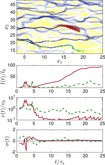
Figure 1: (Left panel) Illustration of the evolution of length (rescaled) and orientation of material strips along streamlines in a steady $d=2$ dimensional divergence-free random flow Le Borgne et al. (2013). The color scales illustrate the velocity magnitude decreasing from blue to yellow. Strips are drawn along streamlines at equidistant times. We observe persistent stretching in low velocity zones. This is reflected in the right panel, which illustrates (top) strip elongations $\ell(t)$ for two distinct streamlines characterized by high (green dashed) and low (red solid) velocities, (middle) strip velocity time series, and (bottom) shear deformation corresponding to the strip evolutions illustrated in the left panel by the same colors.

Thus, we can formulate the evolution equation (5) of a material strip in streamline coordinates as

$$dz_{1}(s) =\frac{dv_{s}(s)}{v_{s}(s)}z_{1}(s)+\frac{\sigma(s)}{v_{s}(s)}z_{2}(s)ds$$ (7a)

$$dz_{2}(s) =-\frac{dv_{s}(s)}{v_{s}(s)}z_{2}(s),$$ (7b)

where we used (2) to express ${\mathbf{z}}(t)={\mathbf{z}}[s(t)]$ in terms of the distance along the streamline. The system (7) can be integrated to

$$z_{1}(s) =\frac{v_{s}(s)}{v_{s}(0)}\left[z_{1}(0)+z_{2}(0)\int\limits_{0}^{s}ds^{\prime}\sigma(s^{\prime})\frac{v_{s}(0)^{2}}{v_{s}(s^{\prime})^{3}}\right]$$ (8a)

$$z_{2}(s) =\frac{v_{s}(0)}{v_{s}(s)}z_{2}(0).$$ (8b)

Note that the deformation tensor $\mathbf{F}(t)$ in the streamline system has also an upper triangular form. Its components can be directly read off the system (8). The angle of the strip ${\mathbf{z}}(t)$ with respect to the streamline orientation is denoted by $\phi(t)$ such that $z_{1}(t)=\ell(t)\cos[\phi(t)]$ and $z_{2}(t)=\ell(t)\sin[\phi(t)]$. The initial strip length and angle are denoted by $\ell_{0}$ and $\phi_{0}$. The strip length is given by $\ell(t)\equiv\ell[s(t)]$ with $\ell(s)=[z_{1}(s)^{2}+z_{2}(s)^{2}]^{1/2}$.

The system (8) is of general validity for $d=2$ dimensional steady flow fields. It reveals the mechanisms that lead to an increase of the strip elongation, which is fully determined by the shear deformation $\sigma(s)$ and the velocity $v_{s}(s)$ along the streamline. For a strip that is initially aligned with the streamline, $z_{2}(0)=0$, the elongation is $\ell(s)=z_{2}(0)v_{s}(s)/v_{s}(0)$ because $z_{2}(s)\equiv 0$ remains zero. This means $\ell(s)$ merely fluctuates without a net increase . Only if the strip is oriented away from the streamline can the streamwise velocity fluctuations be converted into stretching. This identifies the integral term in (8a) as the dominant contribution to the strip elongation. It represents the interaction of shear deformation and velocity with a linear contribution from the shear rate and a non-linear contribution from velocity as $1/v_{s}(s)^{3}$, which may be understood as follows. One power comes from the divergence of streamlines in low velocity zones, which increases $z_{2}(s)$ and thus leads to enhanced shear deformation. The second power is purely kinematic due to the weighting with the residence time in a streamline segment. The third power stems from the fact that shear deformation in low velocity segments is applied while the strip is compressed in streamline direction. This deformation is then amplified as the strip is stretched due to velocity increase. As a result of this non-linear coupling, the history of low velocity episodes has a significant impact on the net stretching as quantified by the integral term in (8b). This persistent effect is superposed with the local velocity fluctuations. These mechanisms are illustrated in Figure 1. While for a stratified flow field with ${\mathbf{u}}({\mathbf{x}})={\mathbf{u}}(x_{2})$ velocity and shear deformation are constant along a streamline such that $\ell(t)=[(z_{1}(0)+z_{2}(0)\sigma t)^{2}+z_{2}(0)^{2}]^{1/2}$, that is, it increases linearly with time, stretching can in general be sub- or superlinear, depending on the duration of low velocity episodes. In the following, we will analyze these behaviors in order to identify and quantify the origins of algebraic stretching.

To investigate the consequences of the non-linear coupling between shear and velocity on the emergence of su-exponential stretching, we cast the dynamics (8) in the framework of a coupled CTRW. Thus, we assume that the random flow field is stationary and ergodic and consider fluid elements that move along ergodic streamlines . We consider random flows ${\mathbf{u}}({\mathbf{x}})$ whose velocity fluctuations are controlled by a characteristic length scale. We focus on the impact of broad velocity point distributions rather than on that of long range correlation Bouchaud and Georges (1990); Dentz and Bolster (2010). This is particularly relevant for porous media flows. It has been observed at the pore and Darcy scales that the streamwise velocity, that is, the velocity measured equidistantly along a streamline follows a Markov process Le Borgne et al. (2008b, a); Kang et al. (2011); De Anna et al. (2013); Edery et al. (2014). Thus, if we choose a coarse-graining scale that is of the order of the streamwise correlation length $\lambda_{c}$, (2) can be discretized as

$$s_{n+1}=s_{n}+\lambda_{c}, t_{n+1}=t_{n}+\frac{\lambda_{c}}{v_{n}}.$$ (9)

The $v_{n}=v_{s}(s_{n})$ are identical independently distributed random velocities with the probability density function (PDF) $p_{v}(v)$. A result of this spatial Markovianity is that the particle movement follows a continuous time random walk (CTRW) Scher and Lax (1973); Berkowitz and Scher (1997). The PDF of streamwise velocities $p_{v}(v)$ is related to the Eulerian velocity PDF $p_{e}(v)$ through flux weighting as $p_{v}(v)\propto vp_{e}(v)$. The Eulerian velocity PDF in $d=2$ dimensional pore-networks, for example, can be approximated by a Gaussian-shaped distribution, which breaks down for small velocities Araújo et al. (2006). For Darcy scale porous and fractured media the velocity PDF can be characterized by algebraic behaviors at small velocities Berkowitz and Scher (1997); Edery et al. (2014); Kang et al. (2015), which implies a broad distribution of transition times $\tau_{n}=\lambda_{c}/v_{n}$. Note, however, that the proposed CTRW stretching mechanisms is of general nature and valid for any velocity distribution $p_{v}(v)$. Thus, in order to extract the deformation dynamics, we coarse-grain the elongation process along the streamline on the correlation scale $\lambda_{c}$. This gives for the strip coordinates (8)

$$z_{1}(s_{n}) =z_{1}(0)\frac{v_{n}}{v_{0}}+z_{2}(0)\frac{v_{n}v_{0}}{v_{c}^{2}}\sigma_{c}\tau_{v}r_{n}$$ (10a)

$$z_{2}(s_{n}) =z_{2}(0)\frac{v_{0}}{v_{n}},$$ (10b)

with $v_{c}$ and $\sigma_{c}$ a characteristic velocity and shear rate, and $\tau_{v}=\lambda_{c}/v_{c}$ a characteristic advection time. The process $r_{n}$, which results from the integral term in (8a), describes the coupled CTRW

$$r_{n+1}=r_{n}+\frac{v_{c}^{3}}{\sigma_{c}}\frac{\sigma_{n}}{v_{n}^{3}}, t_{n+1}=t_{n}+\frac{\lambda_{c}}{v_{n}}.$$ (11)

The elongation at time $t$ is given by $\ell(t)=[z_{1}(s_{n_{t}})^{2}+z_{2}(s_{n_{t}})^{2}]^{1/2}$. It is observed over several $2d$ flows that the shear rate may be related to the streamwise velocity as $\sigma_{n}=\xi_{n}\sigma_{c}(v_{n}/v_{c})^{\hat{\alpha}}$ with $\hat{\alpha}\approx 1$, $\sigma_{c}$ a characteristic shear rate, and $\xi_{n}$ an identical independent random variable that is equal to $\pm 1$ with equal probability. The average shear rate $\langle\sigma_{n}\rangle=0$ due to the stationarity of the random flow field ${\mathbf{u}}({\mathbf{x}})$. Thus, (11) denotes a coupled CTRW whose increments $\rho_{n}\equiv r_{n+1}-r_{n}$ are related to the transition times $\tau_{n}=\lambda_{c}/v_{n}$ as

$$\rho_{n}=\xi_{n}\left({\tau_{n}}/{\tau_{v}}\right)^{\alpha}, \alpha=3-\hat{\alpha}.$$ (12)

It has the average $\langle\rho_{n}\rangle=0$ and absolute value $|\rho_{n}|=(\tau_{n}/\tau_{v})^{\alpha}$. The joint PDF of the elongation increments $\rho$ and transition times $\tau$ is then given by

$$\psi(\rho,\tau)=\frac{1}{2}\delta\left[|\rho|-(\tau/\tau_{v})^{\alpha}\right]\psi(\tau),$$ (13)

where $\delta(\rho)$ denotes the Dirac delta distribution. The transition time PDF $\psi(\tau)$ is related to the streamwise velocity PDF $p_{v}(v)$ as $\psi(\tau)=\lambda_{c}\tau^{-2}p_{v}(\lambda_{c}/\tau)$.

In the following, we consider a streamwise velocity PDF that behaves as $p_{v}(v)\propto(v/v_{c})^{\beta-1}$ for $v$ smaller than the characteristic velocity $v_{c}$. Such a power-law is a model for the low end of the velocity spectra in disordered media Bouchaud and Georges (1990) and porous media flows Berkowitz et al. (2006); Bijeljic et al. (2011); Edery et al. (2014). Note however that the derived CTRW-based deformation mechanism is valid for any velocity distribution. The relation between the streamwise and Eulerian velocity PDFs, $p_{v}(v)\propto vp_{e}(v)$ implies that $\beta\geq 1$ because $p_{e}(v)$ needs to be integrable in $v=0$. The corresponding transition time PDF $\psi(\tau)$ behaves as $\psi(\tau)\propto(\tau/\tau_{v})^{-1-\beta}$ for $\tau>\tau_{v}=\lambda_{c}/v$ and decreases sharply for $\tau<\tau_{v}$. Due to the constraint $\beta>1$, the mean transition time $\langle\tau\rangle<\infty$ is always finite, which is a consequence of fluid mass conservation. For transport in highly heterogeneous pore Darcy-scale porous media values for $\beta$ between $0$ and $2$ have been reported Berkowitz et al. (2006); Bijeljic et al. (2011). It has been found that decreasing medium heterogeneity leads to a sharpening of the transition time PDF and increase of the exponent $\beta$ Edery et al. (2014) with $\beta>1$. With these definitions, the coupled CTRW (11) describes a Levy walk.

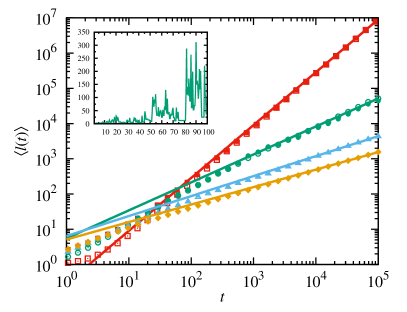
Figure 2: Evolution of the (open symbols) mean elongation $\langle\ell(t)\rangle=\langle[z_{1}(s_{n_{t}})^{2}+z_{2}(s_{n_{t}})^{2}]^{1/2}\rangle$ with $\ell_{n}$ given obtained from numerical Monte-Carlo simulations using (10) and (11) for a uniform distribution of initial strip orientations $\phi\in[-\pi/2,\pi/2]$ and a Gamma PDF of streamwise velocity. The full symbols are obtained from the approximation (14) for (squares) $\beta=3/2$, (circles) $\beta=5/2$, (triangles) $\beta=7/2$ and (rhombi) $\beta=9/2$. The solid lines indicate the late time power-law behaviors of $\langle\ell(t)\rangle\propto t^{3-\beta}$ for $1<\beta<2$, $\langle\ell(t)\rangle\propto t^{2/\beta}$ for $2<\beta<4$, and $\langle\ell(t)\rangle\propto t^{1/2}$ for $\beta>4$. The inset illustrates the evolution of $\ell(t)$ in a single realization of the velocity field $v_{n}$ for $\beta=5/2$ for an initial orientation of $\phi=0$.

Figure 2 shows the evolution of the average elongation $\langle\ell(t)\rangle$ for $\alpha=0$ and different values of $\beta$ obtained from numerical Monte-Carlo simulation using (10) and the Levy walk (11) for the evolution of the strip coordinates based on a Gamma PDF of streamwise velocities . The mean elongation shows a power-law behavior and increases as $\langle\ell(t)\rangle\propto t^{\nu}$. As discussed above, long episodes of small velocity maintain the strip in a favorable shear angle, which leads to a strong stretching. These dynamics are quantified by the Lévy walk process (11), which relates strong elongations to long transition times, i.e., small streamwise velocities, through (12). This is also illustrated in the inset of Figure 2, which shows the elongation of a single material strip. The elongation events increase with increasing time as a consequence of the coupling (12) between stretching and transition time. This is an intrinsic property of a CTRW characterized by a broad $\psi(\tau)$; the transition times increase as time increases, and thus, through the Levy walk coupling also the stretching increments. In fact, the strip length can be approximated by 

$$\ell(t)\approx\ell_{0}+\frac{\sigma_{c}\tau_{v}^{2}\langle v\rangle}{\langle\tau\rangle v_{c}}|z_{2}(0)||r_{n_{t}}|.$$ (14)

The leading behavior of the mean elongation $\langle\ell(t)\rangle$ of a material element is directly related to the mean absolute moment of $r(t)$ as $\langle\ell(t)\rangle\propto\langle|r_{n_{t}}|\rangle$. Thus, even though $r_{n_{t}}$ is in average $0$, the addition of large elongation events in its absolute value $|r(t)|$, which correspond to episodes of low velocities, leads in average to an algebraic increase of $\ell(t)$ as detailed in the following.

The statistics of the Levy walk (11) have been analyzed in detail in Ref. Dentz et al. (2015) for $\alpha>0$ and $\beta>0$. Here, $\beta$ is restricted to $\beta>1$ due to fluid mass conservation. Furthermore, we consider $\alpha\geq 1$. The scaling of the mean absolute moments of $r_{n_{t}}$ depends on the $\alpha$ and $\beta$ regimes.

If the exponent $\beta>2\alpha$, which means a relatively weak heterogeneity, we speak of a weak coupling between the elongation increment $\rho_{n}$ and the transition time $\tau_{n}$ in (12). In this case, the strip elongation behaves as $\langle\ell(t)\rangle\propto t^{1/2}$. We term this behavior here diffusive or normal stretching. For $\alpha=2$ as employed in the numerical simulations this means that $\beta>4$. The coupled Levy-walk (11) reduces essentially to a Brownian motion because the variability of transition times is low so that the coupling does not lead to strong elongation events. Note that scalar dispersion in this $\beta$–range is normal Scher and Lax (1973); Berkowitz et al. (2006).

For strong coupling, this means $\beta<2\alpha$ and thus stronger flow heterogeneity, it has been shown Dentz et al. (2015) that the density of $r_{n_{t}}$ is characterized by two scaling forms, one that characterizes the bulk behavior and a different one for large $r_{n_{t}}$. As a consequence, we need to distinguish the cases of $\beta$ larger and smaller than $\alpha$. Also, the scaling of $|r_{n_{t}}|$ cannot be obtained by dimensional analysis. In fact, $r_{n_{t}}$ has a strong anomalous diffusive character Dentz et al. (2015).

For $\alpha<\beta<2\alpha$ the scaling behavior of the mean elongation is $\langle\ell(t)\rangle\propto t^{\alpha/\beta}$. This means for $\alpha=2$, the stretching exponent $\nu$ is between $1/2$ and $1$, the $\beta$–range is $2<\beta<4$. It interesting to note that scalar dispersion in this range is normal as well. Here, the frequency of low velocity regions is high enough to increase stretching above the weakly coupled case, but not to cause super-diffusive scalar dispersion.

For $1<\beta<\alpha$ in contrast, the mean elongation scales as  Dentz et al. (2015) $\langle\ell(t)\rangle\propto t^{1+\alpha-\beta}$. The stretching exponent is between $1$ and $\alpha$, this means stretching is stronger than for shear flow. The range of scaling exponents $\nu$ of the mean elongation here is $1/2\leq\nu<\alpha$. Specifically, $\alpha\approx 2$ implies that stretching is super-linear for $1<\beta<2$, this means faster than by a pure shear flow, for which $\nu=1$. Here the presence of low velocities in the flow leads to enhanced stretching and at the same time to superdiffusive scalar dispersion.

In summary, we have presented a fundamental mechanism for power-law stretching in random flows through intermittent shear events, which may explain algebraic mixing processes observed across a range of heterogeneous flows. We have shown that the non-linear coupling between streamwise velocities and shear deformation implies that stretching follows Lévy walk dynamics, which explains observed algebraic stretching behaviors that can range from diffusive to super-diffusive scalings, $\langle\ell(t)\rangle\propto t^{\nu}$ with $1/2\leq\nu<2$. The derived coupled stretching CTRW can be parameterized in terms of the Eulerian velocity and deformation statistics and provides a link between anomalous dispersion and fluid deformation. The presented analysis demonstrates that the dynamics of fluid stretching in heterogeneous flow fields is much richer than the paradigmatic linear and exponential behaviors. The non-linear coupling between deformation and shear, The fundamental mechanism of intermittent shear events, which is at the root of non-exponential stretching, is likely present in a broader class of fluid flows.