Generalized minimum dominating set and application in automatic text summarization

Abstract

For a graph formed by vertices and weighted edges, a generalized minimum dominating set (MDS) is a vertex set of smallest cardinality such that the summed weight of edges from each outside vertex to vertices in this set is equal to or larger than certain threshold value. This generalized MDS problem reduces to the conventional MDS problem in the limiting case of all the edge weights being equal to the threshold value. We treat the generalized MDS problem in the present paper by a replica-symmetric spin glass theory and derive a set of belief-propagation equations. As a practical application we consider the problem of extracting a set of sentences that best summarize a given input text document. We carry out a preliminary test of the statistical physics-inspired method to this automatic text summarization problem.

1 Introduction

Minimum dominating set (MDS) is a well-known concept in the computer science community (see review [1]). For a given graph, a MDS is just a minimum-sized vertex set such that either a vertex belongs to this set or at least one of its neighbors belongs to this set. In the last few years researchers from the statistical physics community also got quite interested in this concept, as it is closely related to various network problems such as network monitoring, network control, infectious disease suppression, and resource allocation (see, for example, [2, 3, 4, 5, 6, 7, 8, 9, 10] and review [11]). Constructing an exact MDS for a large graph is, generally speaking, an extremely difficult task and it is very likely that no complete algorithm is capable of solving it in an efficient way. On the other hand, by mapping the MDS problem into a spin glass system with local many-body constraints and then treating it by statistical-physics methods, one can estimate with high empirical confidence the sizes of minimum dominating sets for single graph instances [12, 13]. One can also construct close-to-minimum dominating sets quickly through a physics-inspired heuristic algorithm [12, 13], which might be important for many practical applications.

In the present work we extend the statistical-physics approach of [12, 13] to edge-weighted graphs and study a generalized minimum dominating set problem. Our work is motivated by a practical knowledge-mining problem: extracting a set of sentences to best summarize one or more input text documents [14, 15]. We consider a general graph of vertices and edges, each edge connecting two different vertices and bearing one weight or a pair of weights (see Fig. 1). In the context of text summarization, a vertex represents a sentence of some text documents and an edge weight is the similarity between two sentences. Various data-clustering problems can also be represented as weighted graphs. Given such a weighted graph, our task is then to construct a minimum-cardinality set $\Gamma_{0}$ of vertices such that if a vertex $i$ is not included in $\Gamma_{0}$, the summed weight of the edges from $i$ to vertices in $\Gamma_{0}$ must reach at least certain threshold value $\theta$. The set $\Gamma_{0}$ is referred to as a (generalized) MDS.

We introduce a spin glass model for this generalized MDS problem in Sec. 2 and then describe a replica-symmetric (RS) mean field theory in Sec. 3. A message-passing algorithm BPD (belief-propagation guided decimation) is outlined in Sec. 4, and is then applied to the automatic text summarization problem in Sec. 5. We conclude this work in Sec. 6 and discuss a way of modifying the spin glass model for better treating the text summarization problem.

2 Constraints and a spin glass model

We consider a generic graph $G$ formed by $N$ vertices with indices $i,j,k,\ldots\in\{1,2,\ldots,N\}$ and $M=(c/2)N$ edges between pairs of these vertices (Fig. 1). The constant $c$ is the mean vertex degree of the graph (on average a vertex is attached with $c$ edges). Each edge $(i,j)$ is associated with a pair of non-negative weights $w_{i,j}$ and $w_{j,i}$ which may or may not be equal. The meaning of the edge weights depend on the actual context. For example, $w_{i,j}$ may be interpreted as the extent that vertex $i$ represents vertex $j$; in the symmetric case of $w_{i,j}=w_{j,i}$, we may also interpret $w_{i,j}$ as the similarity between $i$ and $j$. Two vertices $i$ and $j$ are referred to as mutual neighbors if they are connected by an edge $(i,j)$. The set of neighbors of vertex $i$ is denoted as $\partial i$, i.e., $\partial i\equiv\{j\,|\,(i,j)\in G\}$.

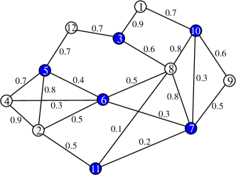
Figure 1: An graph with $N=12$ vertices and $M=21$ weighted edges. In this example the two weights $w_{i,j}$ and $w_{j,i}$ of each edge $(i,j)$ are equal ($w_{i,j}=w_{j,i}$), and the threshold value of each vertex is $\theta=1.0$. The vertex set $\Gamma_{0}=\{3,5,6,7,10,11\}$ is a generalized minimum dominating set for this graph. The summed weight of edges from every vertex $j\notin\Gamma_{0}$ to vertices in $\Gamma_{0}$ is equal to or greater than $\theta$.

Given a graph $G$, we want to construct a vertex set $\Gamma_{0}$ that is as small as possible and at the same time is a good representation of all the other vertices not in this set. Let us assign a state $c_{i}\in\{0,1\}$ to each vertex $i$, $c_{i}=1$ if $i\in\Gamma_{0}$ (referred to as being occupied) and $c_{i}=0$ if $i\notin\Gamma_{0}$ (referred to as being empty). For each vertex $j\notin\Gamma_{0}$ we require that $\sum_{i\in\partial j}c_{i}w_{i,j}\geq\theta$, where $\theta$ is a fixed threshold value. A vertex $j$ is regarded as being satisfied if it is occupied ($c_{j}=1$) or the condition $\sum_{i\in\partial j}c_{i}w_{i,j}\geq\theta$ holds, otherwise it is regarded as being unsatisfied. Therefore there are $N$ vertex constraints in the system. A configuration $(c_{1},c_{2},\ldots,c_{N})$ for the whole graph is referred to as a satisfying configuration if and only if it makes all the vertices to be satisfied (Fig. 1). Constructing such a generalized MDS $\Gamma_{0}$, i.e., a satisfying configuration with the smallest number of occupied vertices, is a $0$–$1$ integer programming problem, but as it belongs to the nondeterministic polynomial-hard (NP-hard) computational complexity class, no algorithm is guaranteed to solve it in polynomial time. We now seek to solve it approximately through a statistical physics approach.

Let us introduce a weighted sum $Z(\beta)$ of all the $2^{N}$ possible microscopic configurations $(c_{1},c_{2},\ldots,c_{N})$ as

$$Z(\beta)=\sum_{c_{1},\ldots,c_{N}}\prod\limits_{j=1}^{N}\biggl{[}\delta_{c_{j}}^{1}e^{-\beta}+\delta_{c_{j}}^{0}\Theta\Bigl{(}\sum\limits_{i\in\partial j}c_{i}w_{i,j}-\theta\Bigr{)}\biggr{]}\;,$$ (1)

where $\delta_{a}^{b}$ is the Kronecker symbol ($\delta_{a}^{b}=1$ if $a=b$ and $\delta_{a}^{b}=0$ if $a\neq b$), and $\Theta(x)$ is the Heaviside step function such that $\Theta(x)=0$ for $x<0$ and $\Theta(x)=1$ for $x\geq 0$. In the statistical physics community, $Z(\beta)$ is known as the partition function and the non-negative parameter $\beta$ is the inverse temperature. Notice a configuration $(c_{1},c_{2},\ldots,c_{N})$ has no contribution to $Z(\beta)$ if it is not a satisfying configuration. If a configuration satisfies all the vertex constraints, it contributes a term $e^{-\beta N_{1}}$ to $Z(\beta)$, where $N_{1}\equiv\sum_{i=1}^{N}c_{i}$ is the total number of occupied vertices. As $\beta$ increases, satisfying configurations with smaller $N_{1}$ values become more important for $Z(\beta)$, and at $\beta\rightarrow\infty$ the partition function is contributed exclusively by the satisfying configurations with the smallest $N_{1}$. For the purpose of constructing a minimum or close-to-minimum dominating set, we are therefore interested in the large-$\beta$ limit of $Z(\beta)$.

3 Replica-symmetric mean field theory

It is very difficult to compute the partition function $Z(\beta)$ exactly, here we compute it approximately using the replica-symmetric mean field theory of statistical physics. This RS mean field theory can be understood from the angle of Bethe-Peierls approximation [16, 17], it can also be derived through loop expansion of the partition function [18, 19].

3.1 Thermodynamic quantities

We denote by $q_{j}^{c_{j}}$ the marginal probability that vertex $j$ is in state $c_{j}\in\{0,1\}$. Due to the constraints associated with vertex $j$ and all its neighboring vertices, the state $c_{j}$ is strongly correlated with those of the neighbors. To write down an approximate expression for $q_{j}^{c_{j}}$, let us assume that the states of all the vertices in set $\partial j$ are independent before the constraint of vertex $j$ is enforced. Under this Bethe-Peierls approximation we then obtain that

$$q^{c_{j}}_{j}\approx\frac{\delta_{c_{j}}^{1}e^{-\beta}\sum\limits_{\{c_{i}\,:\,i\in\partial j\}}\prod\limits_{i\in\partial j}q^{(c_{i},1)}_{i\rightarrow j}+\delta_{c_{j}}^{0}\sum\limits_{\{c_{i}\,:\,i\in\partial j\}}\Theta\Bigl{(}\sum\limits_{i\in\partial j}c_{i}w_{i,j}-\theta\Bigr{)}\prod\limits_{i\in\partial j}q^{(c_{i},0)}_{i\rightarrow j}}{e^{-\beta}\sum\limits_{\{c_{i}\,:\,i\in\partial j\}}\prod\limits_{i\in\partial j}q^{(c_{i},1)}_{i\rightarrow j}+\sum\limits_{\{c_{i}\,:\,i\in\partial j\}}\Theta\Bigl{(}\sum\limits_{i\in\partial j}c_{i}w_{i,j}-\theta\Bigr{)}\prod\limits_{i\in\partial j}q^{(c_{i},0)}_{i\rightarrow j}}\;.$$ (2)

In the above equation, $q_{i\rightarrow j}^{(c_{i},c_{j})}$ is the joint probability that vertex $i$ has state $c_{i}$ and its neighboring vertex $j$ has state $c_{j}$ when the constraint associated with vertex $j$ is not enforced. The product $\prod_{i\in\partial j}q_{i\rightarrow j}^{(c_{i},c_{j})}$ is a direct consequence of neglecting the correlations among vertices in $\partial j$ in the absence of vertex $j$’s constraint. The mean fraction $\rho\equiv N_{1}/N$ of occupied vertices is then obtained through

$$\rho=\frac{1}{N}\sum\limits_{j=1}^{N}q_{j}^{1}\;,$$ (3)

This fraction should be a decreasing function of $\beta$.

We can define the free energy of the system as $F(\beta)=-\frac{1}{\beta}\ln Z(\beta)$. Within the RS mean field theory this free energy can be computed through

$$F\equiv Nf=\sum\limits_{j=1}^{N}f_{j}-\sum\limits_{(i,j)\in G}f_{(i,j)}\;,$$ (4)

where $f$ is the free energy density; and $f_{j}$ and $f_{(i,j)}$ are, respectively, the free energy contribution of a vertex $j$ and an edge $(i,j)$:

$$f_{j} =-\frac{1}{\beta}\ln\biggl{[}e^{-\beta}\sum\limits_{\{c_{i}\,:\,i\in\partial j\}}\prod\limits_{i\in\partial j}q^{(c_{i},1)}_{i\rightarrow j}+\sum\limits_{\{c_{i}\,:\,i\in\partial j\}}\Theta\Bigl{(}\sum_{i\in\partial j}c_{i}w_{i,j}-\theta\Bigr{)}\prod\limits_{i\in\partial j}q^{(c_{i},0)}_{i\rightarrow j}\biggr{]}\;,$$ (5a)

$$f_{(i,j)} =-\frac{1}{\beta}\ln\biggl{[}\sum\limits_{c_{i},c_{j}}q^{(c_{i},c_{j})}_{i\rightarrow j}q^{(c_{j},c_{i})}_{j\rightarrow i}\biggr{]}\;.$$ (5b)

The partition function is predominantly contributed by satisfying configurations with number of occupied vertices $N_{1}\approx N\rho$, namely $Z(\beta)\approx e^{-\rho\beta N}\Omega(\rho)$ with $\Omega(\rho)$ being the total number of satisfying configurations at occupation density $\rho$. Then the entropy density $s(\rho)\equiv\frac{1}{N}\ln\Omega(\rho)$ of the system is computed through

$$s=(\rho-f)\beta\;.$$ (6)

The entropy density is required to be non-negative by definition. If $s(\rho)<0$ as $\rho$ decreases below certain value $\rho_{0}$, then $\Omega(\rho)=e^{Ns(\rho)}\rightarrow 0$ suggests that there is no satisfying configurations with $\rho<\rho_{0}$. We therefore take the value $\rho_{0}$ as the fraction of vertices contained in a minimum dominating set.

3.2 Belief-propagation equation

We need to determine the probabilities $q_{i\rightarrow j}^{(c_{i},c_{j})}$ to compute the thermodynamic densities $\rho$, $f$, and $s$. Following the Bethe-Peierls approximation and similar to Eq. (2), $q_{i\rightarrow j}^{(c_{i},c_{j})}$ is self-consistently determined through

$$q_{i\rightarrow j}^{(0,0)} =\frac{1}{z_{i\rightarrow j}}\sum\limits_{\{c_{k}\,:\,k\in\partial i\backslash j\}}\Theta\Bigl{(}\sum\limits_{k\in\partial i\backslash j}c_{k}w_{k,i}-\theta\Bigr{)}\prod\limits_{k\in\partial i\backslash j}q_{k\rightarrow i}^{(c_{k},0)}\;,$$ (7a)

$$q_{i\rightarrow j}^{(0,1)} =\frac{1}{z_{i\rightarrow j}}\sum\limits_{\{c_{k}\,:\,k\in\partial i\backslash j\}}\Theta\Bigl{(}w_{j,i}+\sum\limits_{k\in\partial i\backslash j}c_{k}w_{k,i}-\theta\Bigr{)}\prod\limits_{k\in\partial i\backslash j}q_{k\rightarrow i}^{(c_{k},0)}\;,$$ (7b)

$$q_{i\rightarrow j}^{(1,0)}=q_{i\rightarrow j}^{(1,1)} =\frac{1}{z_{i\rightarrow j}}e^{-\beta}\prod_{k\in\partial i\backslash j}\Bigl{[}q_{k\rightarrow i}^{(1,1)}+q_{k\rightarrow i}^{(0,1)}\Bigr{]}\;,$$ (7c)

where $\partial i\backslash j$ is the subset of $\partial i$ with vertex $j$ being deleted, and $z_{i\rightarrow j}$ is a normalization constant. Equation (7) is called a belief-propagation (BP) equation in the literature. To find a solution to Eq. (7) we iterate this equation on all the edges of the input graph $G$ (see, for example, [12, 13] or [19] for implementing details). However convergence is not guaranteed to achieve. If the reweighting parameter $\beta$ is small this BP iteration quickly reaches a fixed point; while at large values of $\beta$ we notice that it usually fails to converge (see next subsection).

3.3 Results on Erdös-Rényi random graphs

We first apply the RS mean field theory to Erdös-Rényi (ER) random graphs. To generate an ER random graph, we select $M$ different pairs of edges uniformly at random from the whole set of $N(N-1)/2$ vertex pairs and then connect each selected pair of vertices by an edge. For $N$ sufficiently large there is no structural correlations in such a random graph, and the typical length of a loop in the graph diverges with $N$ in a logarithmic way.

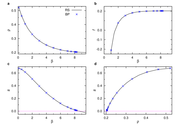
Figure 2: Replica-symmetric mean field results on ER random networks of mean vertex degree $c=10.0$. The symmetric edge weights are drawn from the set $\{0.4,0.5,0.6,0.7,0.8,0.9,1.0\}$ and the vertex threshold value is $\theta=1$. The cross symbols (BP) are results obtained by belief-propagation on a single graph instance of size $N=10^{5}$, while the solid lines (RS) are ensemble-averaged results obtained by population dynamics simulations. (a) Occupation density $\rho$ versus inverse temperature $\beta$; (b) free energy density $f$ versus $\beta$; (c) entropy density $s$ versus $\beta$; (d) entropy density $s$ as a function of $\rho$ obtained by combining data of (a) and (c).

If the two edge weights of every edge $(i,j)$ are equal to the vertex threshold value $\theta$ ($w_{i,j}=w_{j,i}=\theta$), the generalized MDS problem reduces to the conventional MDS problem on an undirected graph, which has been successfully treated in [12]. For example, for ER random graphs with mean vertex degree $c=10.0$ the MDS relative size is $\rho_{0}\approx 0.120$ [12]. On the other hand, if the two edge weights of every edge are strongly non-symmetric such that either $w_{i,j}=\theta$ and $w_{j,i}=0$ (with probability $1/2$) or $w_{i,j}=0$ and $w_{j,i}=\theta$ (also with probability $1/2$), the generalized MDS problem reduces to the conventional MDS problem on a directed graph, which again has been successfully treated in [13] (e.g., at $c=10.0$ the MDS relative size is $\rho_{0}\approx 0.195$).

In this paper, as a particular example, we consider a distribution of edge weights with the following properties: (1) the weights of every edge $(i,j)$ are symmetric, so $w_{i,j}=w_{j,i}$; (2) the edge weights of different edges are not correlated but completely independent; (3) for each edge $(i,j)$ its weight $w_{i,j}$ is assigned the value $0.4\theta$ or $1.0\theta$ with probability $1/12$ each and assigned values in the set $\{0.5\theta,0.6\theta,0.7\theta,0.8\theta,0.9\theta\}$ with equal probability $1/6$ each.

The BP results on the occupation density $\rho$, the free energy density $f$, and the entropy density $s$ are shown in Fig. 2 for a single ER random graph of $N=10^{5}$ vertices and mean degree $c=10.0$. The BP iteration for this this graph instance is convergent for $0\leq\beta\leq 8.3$. The occupation density $\rho$ and the entropy density $s$ both decrease with inverse temperature $\beta$. The entropy density as a function of occupation density, $s(\rho)$, approaches zero at $\rho=\rho_{0}\approx 0.202$, indicating there is no satisfying configurations at occupation density $\rho<\rho_{0}$. The BP results therefore predict that a MDS for this problem instance must contain at least $0.202N$ vertices.

We can also obtain RS mean field results on the thermodynamic densities by averaging over the whole ensemble of ER random graphs (with $N\rightarrow\infty$ and fixed mean vertex degree $c$). This is achieved by population dynamics simulations [16]. We store a population of probabilities $\{q_{i\rightarrow j}^{(c_{i},c_{j})}\}$ and update this population using Eq. (7), and at the same time compute the densities of thermodynamic quantities. A detailed description on the implementation can be found in section 4.3 of [12]. The ensemble-averaged results for the ER random network ensemble of $c=10.0$ and $N\rightarrow\infty$ are also shown in Fig. 2. These results are in good agreement with the BP results obtained on the single graph instance.

Through the RS population dynamics simulations we can estimate the ensemble-averaged value of $\rho_{0}$ (the minimum fraction of occupied vertices) by the equation $s(\rho_{0})=0$. The value of $\rho_{0}$ obtained in such a way decreases with mean vertex degree $c$ continuously, see Fig. 3 (solid line).

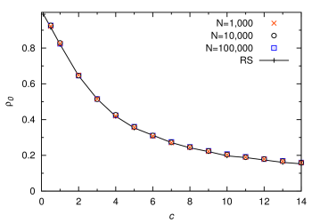
Figure 3: The relative size $\rho_{0}$ of minimum dominating sets for ER random graphs of mean vertex degree $c$. The edge weight distribution for these random graphs are the same as that of Fig. 2, and the vertex threshold value $\theta=1.0$. The solid-line connected plus symbols are the predictions of the RS mean field theory, while the results obtained by the BPD algorithm at $\beta=8.0$ are drawn as cross symbols (for graph size $N=10^{3}$), circles ($N=10^{4}$), and squares ($N=10^{5}$). Each BPD data point is the result of a single run on one graph instance.

4 Belief-propagation-guided decimation algorithm

For $\beta$ sufficiently large, the marginal occupation probability $q_{j}^{c_{j}}$ obtained by Eq. (2) tells us the likelihood of each vertex $j$ to belong to a minimum dominating set. This information can serve as a guide for constructing close-to-minimum dominating sets. Based on the BP equation (2) we implement a simple belief-propagation-guided decimation (BPD) algorithm as follows. Starting from an input graph $G$ and an empty vertex set $\Gamma$, at each step we (1) iterate the BP equation for a number of repeats and then estimate the occupation probability $q_{j}^{1}$ for all the vertices $j$ not in $\Gamma$; and (2) add a tiny fraction (e.g., $1\%$) of those vertices $j$ with the highest values of $q_{j}^{1}$ into the set $\Gamma$ and set their state to be $c_{j}=1$; (3) then simplify the graph and repeat the operations (1)–(3) on the simplified graph, until $\Gamma$ becomes a dominating set.

The detailed implementation of this BPD algorithm is the same as described in section 5 of [12]. Here we only need to emphasize one new feature: after a vertex $i$ is newly occupied, the threshold value (say $\theta_{j}$) of every neighboring vertex $j$ should be updated as $\theta_{j}\leftarrow(\theta_{j}-w_{i,j})$, and if this updated $\theta_{j}$ is non-positive then vertex $j$ should be regarded as being satisfied.

For the same graph of Fig. 2, a single trial of this BPD algorithm at $\beta=8.0$ results in a dominating set of size $21009$, which is very close to the predicted MDS size by the RS mean field theory. Equally good performance of the BPD algorithm is also achieved on other ER random graphs with mean vertex degree $c$ ranging from $c=0.5$ to $c=14$ (see Fig. 3), suggesting that the BPD algorithm is able to construct a dominating set which is very close to a MDS. We emphasize that in the BPD algorithm we do not require the BP iteration to converge.

5 Application: Automatic text summarization

Automatic text summarization is an important issue in the research field of natural language processing [14]. One is faced with the difficult task of constructing a set of sentences to summarize a text document (or a collection of text documents) in a most informative and efficient way. Here we extend the initial idea of Shen and Li [15] and consider this information retrieval problem as a generalized minimum dominating set problem.

We represent each sentence of an input text document as a vertex and connect two vertices (say $i$ and $j$) by an weighted edge, with the symmetric edge weight $w_{i,j}$ ($=w_{j,i}$) being equal to the similarity of the two corresponding sentences. Before computing the edge weight a pre-treatment is applied to all the sentences to remove stop-words (such as ‘a’, ‘an’, ‘at’, ‘do’, ‘but’, ‘of’, ‘with’) and to transform words to their prototypes according to the WordNet dictionary [20] (e.g., ‘airier’ $\rightarrow$ ‘airy’, ‘fleshier’ $\rightarrow$ fleshy, ‘are’ $\rightarrow$ ‘be’, ‘children’ $\rightarrow$ child, ‘looking’ $\rightarrow$ ‘look’). There are different ways to measure sentence similarity, here we consider a simple one, the cosine similarity [21]. To compute the cosine similarity, we map each sentence $i$ to a high-dimensional vector $\vec{S}_{i}$, the $k$-th element of which is just the number of times the $k$-th word of the text appears in this sentence. Then the edge weight between vertices $i$ and $j$ is defined as

$$w_{i,j}=\frac{\vec{S}_{i}\cdot\vec{S}_{j}}{\sqrt{\vec{S}_{i}\cdot\vec{S}_{i}}\sqrt{\vec{S}_{j}\cdot\vec{S}_{j}}}\;.$$ (8)

To give a simple example, let us consider a document with only two sentences ‘Tom is looking at his children with a smile.’ and ‘These children are good at singing.’. The word set of this document is {Tom, be, look, child, smile, good, sing}, and the vectors for the two sentences are $\vec{S}_{1}=(1,1,1,1,1,0,0)$ and $\vec{S}_{2}=(0,1,0,1,0,1,1)$, respectively. The cosine similarity $w_{12}$ between these two sentences is then $w_{12}=\frac{2}{\sqrt{5}\sqrt{4}}\approx 0.447$.

We first test the performance of the BPD algorithm on $32$ short English text documents of different lengths (on average a document has $17.7$ sentences). We compare the outputs from the BPD algorithm with the key sentences manually selected by the first author. For each text document we denote by $B$ and $\tilde{B}$ the set of key sentences selected by human inspection and by the algorithm, respectively. On average the set $B$ of human inspection contains a fraction $\rho=0.226$ of the sentences in the input text document. Then we define the coverage ratio $R_{cov}$ and the difference ratio $R_{dif}$ between $B$ and $\tilde{B}$ as

$$R_{cov}=\frac{\bigl{|}B\cap\tilde{B}\bigr{|}}{\bigl{|}B\bigr{|}}\;,\quad\quad\quad R_{dif}=\frac{\bigl{|}\tilde{B}-B\bigl{|}}{\bigl{|}\tilde{B}\bigr{|}}\;,$$ (9)

where $(\tilde{B}-B)$ denotes the set of sentences belonging to $\tilde{B}$ but not to $B$. The ratio $R_{cov}$ quantifies the probability of a manually selected key sentence also being selected by the algorithm, while the ratio $R_{dif}$ quantifies the extent that a sentence selected by the algorithm does not belong to the set of manually selected key sentences.

Table 1: Averaged performances of the BPD algorithm ($\beta=8.0$), the PR (PageRank) algorithm, and the AP (affinity-propagation) algorithm on $32$ English text documents (average number of sentences per document $17.7$). For BPD the vertex threshold is set to $\theta=0.6$ (BPD_0.6), $\theta=0.8$ (BPD_0.8) and $\theta=1.0$ (BPD_1.0). For PR the fraction of sentences selected is $25\%$ (PR_25%), $30\%$ (PR_30%), and $40\%$ (PR_40%). For AP the adjustable parameter is set to be $w_{i,i}=0.0$ (AP_0.0) and $w_{i,i}=0.2$ (AP_0.2). $\rho$ is the fraction of representative sentences chosen by the algorithm, and $R_{cov}$ and $R_{dif}$ are two performance measures defined by Eq. (9). The average fraction of representative sentences constructed by human inspection is $\rho=0.226$.

	BPD0.6	BPD0.8	BPD1.0	PR25%	PR30%	PR40%	AP0.0	AP0.2
$\rho$	$0.44$	$0.48$	$0.56$	$0.27$	$0.32$	$0.42$	$0.17$	$0.39$
$R_{cov}$	$39.9\%$	$47.2\%$	$49.6\%$	$30.0\%$	$41.7\%$	$50.6\%$	$15.6\%$	$39.3\%$
$R_{dif}$	$79.4\%$	$78.6\%$	$80.2\%$	$74.2\%$	$71.4\%$	$72.2\%$	$76.3\%$	$77.4\%$

We also apply two other summarization algorithms to the same set of text documents, one is the PageRank (PR) algorithm [22, 23, 24], and the other is the Affinity-Propagation (AP) algorithm [25]. PageRank is based on the idea of random walk on a graph, and it offers an efficient way of measuring vertex significance. The importance $P_{i}$ of a vertex $i$ is determined by the following self-consistent equation

$$P_{i}=(1-p)\frac{1}{N}+p*\sum_{j\in\partial i}P_{j}\frac{w_{j,i}}{\sum_{k\in\partial j}w_{j,k}}\;,$$ (10)

where $p$ is the probability to jump from one vertex to a neighboring vertex (we set $p=0.85$ following [22]). Those vertices $i$ with high values of $P_{i}$ are then selected as the representative vertices.

On the other hand, Affinity-Propagation is a clustering algorithm: each vertex either selects a neighboring vertex as its exemplar or serves as an exemplar for some or all of its neighbors [25]. For any pair of vertices $i$ and $j$, the responsibility $r_{i,j}$ of $j$ to $i$ and the availability $a_{i,j}$ of $j$ to $i$ are determined by the following set of iterative equations:

$$r_{i,j} =w_{i,j}-\max_{k\neq j}\bigl{\{}a_{i,k}+w_{i,k}\bigr{\}}\;,$$ (11a)

$$a_{i,j} =\min\Bigl{[}0,\;r_{j,j}+\sum_{k\neq i,j}\max\bigl{[}0,\,r_{k,j}\bigr{]}\Big{]}\;,$$ (11b)

$$a_{j,j} =\sum_{i\neq j}\max\bigl{[}0,\;r_{i,j}\bigr{]}\;.$$ (11c)

In Eq. (11a) $w_{i,j}$ is the weight of edge $(i,j)$ for $i\neq j$, and $w_{i,i}$ is an adjustable parameter which affects the final number of examplars. We iterate the AP equation (11) on the sentence graph starting from the initial condition of $r_{i,j}=a_{i,j}=0$ and, after convergence is reached, then consider all the vertices $i$ with positive values of $(r_{i,i}+a_{i,i})$ as the examplar vertices.

For the $32$ short text documents used in our preliminary test, the comparative results of Table 1 do not distinguish much the three heuristic algorithms, yet it appears that PageRank performs slightly better than BPD and AP. When the fraction of extracted sentences is $\rho=0.42$, the coverage ratio reached by PR is $R_{cov}=0.51$ and the difference ratio is $R_{dif}=0.72$, while $R_{cov}=0.40$ and $R_{dif}=0.79$ for BPD at $\rho=0.44$ and $R_{cov}=0.39$ and $R_{dif}=0.77$ for AP at $\rho=0.39$.

We then continue to evaluate the performance of the belief-propagation approach on a benchmark set of longer text documents, namely the DUC (Document Understanding Conference) data set used in [24]. We examine a total number of $533$ text documents from the DUC 2002 directory [26]. The average number of sentences per document is about $28$ and the average number of words per sentence is about $20$.

The DUC data set offers, for each of these text documents, two sets $B$ of representative sentences chosen by two human experts, the total number of words in such a set $B$ being $\approx 100$. The PageRank algorithm (PR¹⁰⁰) and one version of the BPD algorithm (BPD${}_{\theta}^{100}$, $\theta=0.6$ or $\theta=1.0$) also construct a set $\tilde{B}$ of sentences for each of these documents under the constraint that the total number of words in $\tilde{B}$ should be about $100$. In another version of the BPD algorithm (BPD_θ) the restriction on the words number in $\tilde{B}$ is removed. We follow the DUC convention and use the toolkit ROUGE [27] to evaluate the agreement between $\tilde{B}$ and $B$ in terms of Recall, Precision, and F-score:

$$\mathrm{Recall} =\frac{\sum\limits_{\mathrm{word}\in B}\min\bigl{[}C(\mathrm{word}),\tilde{C}(\mathrm{word})\bigr{]}}{\mathrm{WordsNum}(B)}\;,$$ (12a)

$$\mathrm{Precision} =\frac{\sum\limits_{\mathrm{word}\in B}\min\bigl{[}C(\mathrm{word}),\tilde{C}(\mathrm{word})\bigr{]}}{\mathrm{WordsNum}(\tilde{B})}\;,$$ (12b)

$$\mathrm{Fscore} =\frac{2\times\mathrm{Precision}\times\mathrm{Recall}}{\mathrm{Precision}+\mathrm{Recall}}\;.$$ (12c)

where $C(\mathrm{word})$ is the total number of times a given word appears in the summary $B$, and $\tilde{C}(\mathrm{word})$ is the number of times this word appears in the summary $\tilde{B}$; $\mathrm{WordsNum}(B)$ is the total number of words in the summary $B$ and similarly for $\mathrm{WordsNum}(\tilde{B})$.

Table 2: Averaged performances of the BPD algorithms BPD${}_{\theta}^{100}$ ($\theta=0.6$ or $\theta=1.0$) and BPD_θ ($\theta=1.0$) and the PageRank algorithm PR¹⁰⁰ on the $533$ text documents of DUC 2002 [26]. The Precision, Recall, and F-score values are obtained by averaging over the results of individual text documents. The inverse temperature of BPD is fixed to be $\beta=8.0$.

	PR100	BPD${}_{0.6}^{100}$	BPD${}_{1.0}^{100}$	BPD1.0
Recall	$0.455$	$0.249$	$0.264$	$0.727$
Precision	$0.407$	$0.396$	$0.410$	$0.256$
Fscore	$0.429$	$0.303$	$0.318$	$0.359$

The comparative results for the DUC 2002 data set are shown in Table 2. We notice that BPD_1.0 ($\theta=1.0$) has the highest Recall value of $0.727$, namely the summary obtained by this algorithm contains most of contents in the summary of human experts, but its Precision value of $0.256$ is much lower than that of the PR¹⁰⁰ algorithm, indicating that the BPD algorithm add more sentences into the summary than the human experts do. In terms of the F-score which balances Recall and Precision (the last row of Table 2) we conclude that PageRank also performs a little bit better than BPD for the DUC 2002 benchmark.

The generalized MDS model for the text summarization problem aims at a complete coverage of an input text document. It is therefore natural that the summary constructed by BPD contains more sentences than the summary constructed by the human experts (which may only choose the sentences that best summarize the key points of a text document). All the tested documents in the present work are rather short, which may make the advantages of the BPD message-passing algorithm difficult to be manifested. More work needs to be done to test the performance of the BPD algorithm on very long text documents.

6 Outlook

In this paper we presented a replica-symmetric mean field theory for the generalized minimum dominating set problem, and we considered the task of automatic text summarization as such a MDS problem and applied the BPD message-passing algorithm to construct a set of representative sentences for a text document. When tested on a set of short text documents the BPD algorithm has comparable performance as the PageRank and the Affinity-Propagation algorithms. We feel that the BPD approach will be most powerful for extracting sentences out of lengthy text documents (e.g., scientific papers containing thousands of sentences). We hope that our work will stimulate further efforts on this important application.

The belief-propagation based method for the automatic text summarization problem might be improved in various ways. For example, it may not be necessary to perform the decimation step, rather one may run BP on the input sentence graph until convergence (or for a sufficient number of rounds) and then return an adjustable fraction $\rho$ of the sentences $i$ according to their estimated occupation probabilities $q_{i}^{1}$.

One may also convert the text summarization problem to other generalized MDS problems. A particularly simple but potentially useful one can be constructed as follows: we first construct a bi-partite graph formed by words, sentences, and the links between words and sentences (see Fig. 4); we then construct a minimum-sized dominating set of sentences $\Gamma$ such that every word of the whole bipartite graph must appear in at least $n$ ($n\geq 1$) of the sentences of $\Gamma$. Such a generalized MDS problem can be studied by slightly modifying the BP equation Eq. (7). We notice that this alternative construction has the advantage of encouraging diversity in the selected representative sentences.

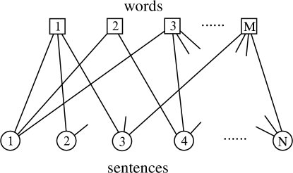
Figure 4: The word–sentence graph representation for a text document. The $M$ words and $N$ sentences of an input text document are denoted by squares and circles, respectively, and a link between a word $a$ and a sentence $i$ is drawn if and only if word $a$ appears in sentence $i$. To get a set $\Gamma$ of representative sentences we may require that each word must be connected to at least $n$ ($n\geq 1$) sentences of the set $\Gamma$.

We thank Jin-Hua Zhao and Yusupjan Habibulla for helpful discussions. This research is partially supported by the National Basic Research Program of China (grant number 2013CB932804) and by the National Natural Science Foundation of China (grand numbers 11121403 and 11225526).

References

References

- [1] Haynes T W, Hedetniemi S T and Slater P J 1998 Fundamentals of Domination in Graphs (New York: Marcel Dekker)
- [2] Echenique P, Gómez-Gardeñes J, Moreno Y and Vázquez A 2005 Distance- covering problems in scale-free networks with degree correlations Phys. Rev. E 71 035102(R)
- [3] Dall’Asta L, Pin P and Ramezanpour A 2009 Statistical mechanics of maximal independent sets Phys. Rev. E 80 061136
- [4] Dall’Asta L, Pin P and Ramezanpour A 2011 Optimal equilibria of the best shot game J. Public Economic Theor. 13 885–901
- [5] Yang Y, Wang J and Motter A E 2012 Network observability transitions Phys. Rev. Lett. 109 258701
- [6] Molnár Jr. F, Sreenivasan S, Szymanski B K and Korniss K 2013 Minimum dominating sets in scale-free network ensembles Sci. Rep. 3 1736
- [7] Nacher J C and Akutsu T 2013 Analysis on critical nodes in controlling complex networks using dominating sets In International Conference on Signal-Image Technology & Internet-Based Systems (Kyoto) 649–654
- [8] Takaguchi T, Hasegawa T and Yoshida Y 2014 Suppressing epidemics on networks by exploiting observer nodes Phys. Rev. E 90 012807
- [9] Wuchty S 2014 Controllability in protein interaction networks Proc. Natl. Acad. Sci. USA 111 7156–7160
- [10] Wang H, Zheng H, Browne F and Wang C 2014 Minimum dominating sets in cell cycle specific protein interaction networks In Proceedings of International Conference on Bioinformatics and Biomedicine (IEEE) 25–30
- [11] Liu Y Y and Barabási A L 2015 Control principles of complex networks arXiv:1508.05384
- [12] Zhao J H, Habibulla Y and Zhou H J 2015 Statistical mechanics of the minimum dominating set problem J. Stat. Phys. 159 1154–1174
- [13] Habibulla Y, Zhao J H and Zhou H J 2015 The directed dominating set problem: Generalized leaf removal and belief propagation Lect. Notes Comput. Sci. 9130 78–88
- [14] Mani I 1999 Advances in Automatic Text Summarization (Cambridge, MA: MIT Press)
- [15] Shen C and Li T 2010 Multi-document summarization via the minimum dominating set In Proceedings of the 23rd International Conference on Computational Linguistics (Beijing) (Association for Computational Linguistics) 984–992
- [16] Mézard M and Parisi G 2001 The bethe lattice spin glass revisited Eur. Phys. J. B 20 217–233
- [17] Mézard M and Montanari A 2009 Information, Physics, and Computation (New York: Oxford Univ. Press)
- [18] Zhou H J and Wang C 2012 Region graph partition function expansion and approximate free energy landscapes: Theory and some numerical results J. Stat. Phys. 148 513–547
- [19] Zhou H J 2015 Spin Glass and Message Passing (Beijing: Science Press)
- [20] Fellbaum C 1998 WordNet: an electronic lexical database (Cambridge, MA: MIT Press)
- [21] Singhal A 2001 Modern information retrieval: a brief overview IEEE Data Engineering Bulletin 24 35–43
- [22] Brin S and Page L 1998 The anatomy of a large-scale hypertextual web search engine Computer Networks and ISDN Systems 30 107–117
- [23] Mihalcea R and Tarau P 2004 Textrank: Bringing order into texts In Preceedings of the Conference on Empirical Methods in Natural Language Processing (Barcelona) (Association for Computational Linguistics) 404–411
- [24] Erkan G and Radev D R 2004 Lexrank: Graph-based lexical centrality as salience in text summarization J. Artifical Intelligence Res. 22 457–479
- [25] Frey B J and Dueck D 2007 Clustering by passing messages between data points Science 315 972–976
- [26] Document Understanding Conference 2002 http://www-nlpir.nist.gov/projects/duc
- [27] Lin C Y 2004 Rouge: a package for automatic evaluation of summaries In Preceedings of the ACL-04 Workshop: Text Summarization Branches Out (Barcelona) (Association for Computational Linguistics) 74–81