Bjorken flow in one-dimensional relativistic magnetohydrodynamics with magnetization

Abstract

We study the one-dimensional, longitudinally boost-invariant motion of an ideal fluid with infinite conductivity in the presence of a transverse magnetic field, i.e., in the ideal transverse magnetohydrodynamical limit. In an extension of our previous work Roy et al., [Phys. Lett. B 750, 45 (2015)], we consider the fluid to have a non-zero magnetization. First, we assume a constant magnetic susceptibility $\chi_{m}$ and consider an ultrarelativistic ideal gas equation of state. For a paramagnetic fluid (i.e., with $\chi_{m}>0$), the decay of the energy density slows down since the fluid gains energy from the magnetic field. For a diamagnetic fluid (i.e., with $\chi_{m}<0$), the energy density decays faster because it feeds energy into the magnetic field. Furthermore, when the magnetic field is taken to be external and to decay in proper time $\tau$ with a power law $\sim\tau^{-a}$, two distinct solutions can be found depending on the values of $a$ and $\chi_{m}$. Finally, we also solve the ideal magnetohydrodynamical equations for one-dimensional Bjorken flow with a temperature-dependent magnetic susceptibility and a realistic equation of state given by lattice-QCD data. We find that the temperature and energy density decay more slowly because of the non-vanishing magnetization. For values of the magnetic field typical for heavy-ion collisions, this effect is, however, rather small. Only for magnetic fields which are about an order of magnitude larger than expected for heavy-ion collisions, the system is substantially reheated and the lifetime of the quark phase might be extended.

I Introduction

It has recently been pointed out that extremely strong magnetic fields are produced in relativistic heavy-ion collisions. In general, their magnitde grows approximately linearly with the centre-of-momentum energy of the colliding nucleons Bzdak:2011yy ; Deng:2012pc ; Li:2016tel , and reaches $B\sim 10^{18}-10^{19}$ G in Au-Au collisions at $\sqrt{s_{NN}}=200$ GeV. In these collisions a new form of hot and dense nuclear matter is created, commonly known as quark-gluon plasma (QGP) Gyulassy:2004zy . In the QGP, quarks are deconfined and chiral symmetry is restored, such that quarks are (approximately) massless and have definite chirality and helicity. Thus, in the presence of very strong magnetic fields, quarks will be polarized and will move preferentially in the direction parallel (or antiparallel) to the magnetic field. Therefore, if the numbers of left- and right-handed quarks are not equal, a net charge current will be induced, a phenomenon known as “chiral magnetic effect” (CME) Kharzeev:2007jp ; Fukushima:2008xe . As well as charge currents, a chiral current can also be induced by the magnetic field and gives rise to the “chiral separation effect” (CSE). Combining these two effects, a density wave is expected to be induced by magnetic fields, called “chiral magnetic wave” (CMW) Kharzeev:2010gd , which might break the degeneracy between the elliptic flows of $\pi^{\pm}$ Burnier:2011bf . Recently, it has been found that these phenomena can be interpreted in the language of the Berry phase and effective chiral kinetic equations, which can be obtained by the path-integral method Stephanov:2012ki ; Chen:2013iga ; Chen:2014cla , Hamiltonian approaches Son:2012wh ; Son:2012zy , and quantum kinetic theory via Wigner functions Gao:2012ix ; Chen:2012ca ; for reviews and additional references see Refs. Bzdak:2012ia ; Kharzeev:2013ffa ; Kharzeev:2015kna ; Pu:Review2015 .

A possible origin of CME, CSE, and CMW is the chiral anomaly, which is topologically invariant. Thus, these effects are not expected to be significantly modified when considering interactions between particles. In contrast, there are also several interesting phenomena dominated by the interactions. For example, instead of a strong magnetic field, a chiral current and density wave can also be induced by an electric field, the so-called “chiral electric separation effect” (CESE) Huang:2013iia ; Pu:2014cwa ; Jiang:2014ura ; Pu:2014fva . Similarly, adding an electric field perpendicular to the magnetic field, a chiral Hall current is expected, called “chiral Hall-separation effect” (CHSE) Pu:2014fva , which might cause an asymmetric charge and chirality distribution in rapidity. These phenomena have drawn considerable attention within the study of hot and dense matter under the influence of strong magnetic fields.

A very popular and successful tool to describe heavy-ion collision dynamics is relativistic hydrodynamics [see, e.g., Refs. Romatschke2007 ; Luzum2008 ; Song2008b ; Song:2008si ; Schenke:2011bn ; Roy:2012jb ; Niemi:2012ry ; Rezzolla2013 ]. In order to study some of the phenomena mentioned above within a hydrodynamical approach, the latter needs to be extended to include magnetic fields, i.e., one has to develop and apply a relativistic magnetohydrodynamical (MHD) framework. Although the magnetic field created in heavy-ion collisions rapidly decays in the vacuum Kharzeev:2007jp and might become very small even before the system reaches local thermal equilibrium, some recent studies have shown that its decay might be substantially delayed in the presence of an electrically conducting medium Gursoy:2014aka ; Zakharov:2014dia ; Tuchin:2013apa . Thus, it is still presently unclear whether the effect of magnetic fields on the dynamics of a heavy-ion collision can be neglected or needs to be taken properly into account.

In analogy with our previous work Roy:2015kma (hereafter paper I), we define the dimensionless quantity, $\sigma=B^{2}/e$, to measure the relative importance of the magnetic field, with $B$ being the magnitude of the magnetic field (measured in units of GeV²) and $e$ the energy density of the fluid. Clearly, for regions where $\sigma\gtrsim 1$, the effect of the magnetic fields cannot be ignored. Interestingly, in a typical mid-central Au-Au collision (e.g., with impact parameter $\sim 10$ fm at $\sqrt{s_{NN}}=200$ GeV), the average magnetic field is $\sim 10\,m_{\pi}^{2}$ Bzdak:2011yy ; Deng:2012pc , with $m_{\pi}$ the pion mass, and the energy density is $\sim 10$ GeV fm^-3, thus giving $\sigma\sim 0.5$. Furthermore, event-by-event simulations show that in certain events $\sigma$ could be even much larger than $1$ in certain regions Roy:2015coa . Therefore, it is still very important to investigate relativistic MHD, ideally with a numerical code solving the equations in 3+1 dimensions.

Before starting to investigate MHD numerically, it is worth while to search for analytic solutions in some simple, but nevertheless realistic test cases. In paper I we have considered one-dimensional, longitudinally boost-invariant Bjorken flow Bjorken:1982qr with a transverse magnetic field and in ideal MHD, i.e., for infinite electrical conductivity and without dissipative effects. Quite remarkably, we found that under these conditions the decay of the energy density is the same as in the case without magnetic field. The reason is that, for a transverse magnetic field, $B/s$ (where $s$ is the entropy density) is conserved and the magnetic field is advected with the fluid, as a manifestation of the "frozen-flux theorem" well-known from astrophysics and plasma physics Rezzolla2013 ; Landau .

In paper I we have neglected the effect of a nonzero magnetization of the QGP. In this work, we extend our previous study to include a nonzero magnetization for the scenario of a pure Bjorken flow. The final goals are those of improving the theoretical understanding of the MHD evolution of the QGP, but also of determining how the magnetization of the QGP may have an influence on measurable quantities, as recently suggested in Ref. Bali:2013owa in relation to the value of the elliptic flow parameter $v_{2}$.

Within a linear approximation, the magnetization effect can be described through the magnetic susceptibility $\chi_{m}$, which is the ratio of the magnetic polarization to the magnetic field. Interestingly, numerous studies, e.g., from lattice QCD Bali:2013owa ; Bonati:2013lca ; Bonati:2013qra ; Levkova:2013qda ; Bonati:2013vba ; Orlovsky:2014cta ; Bali:2014kia and from perturbative QCD Kamikado:2014bua , using the Sakai-Sugimoto model Bergman:2008sg , the functional renormalization group Kamikado:2014bua , or other models Cherman:2008eh ; Steinert:2013fza ; Kabat:2002er ; Orlovsky:2014cta ; Anber:2013tra ; Tawfik:2014hwa , have all suggested that in a confined phase (hadron phase) the medium is diamagnetic, i.e., with $\chi_{m}<0$, while in the deconfined QGP phase it is paramagnetic, i.e., with $\chi_{m}>0$. As a result, by simply choosing different signs of $\chi_{m}$, we can investigate the dynamics of different phases with nonzero magnetization.

In principle, the magnetic susceptibility $\chi_{m}$ of the QGP is a function of the temperature and of the magnitude of the magnetic field. In practice, however, the variation of $\chi_{m}$ is very small in the experimentally accessible region of temperatures and magnetic fields. For example, from lattice-QCD calculations Bali:2013owa ; Bonati:2013qra [see also Ref. Orlovsky:2014cta ], for $(eB)^{2}=0.007-0.2$ GeV² and $T=100-350$ MeV, the susceptibility is in the range $0\lesssim\chi_{m}\lesssim 0.05$ [note that a prefactor $4\pi\alpha$ is required to convert the values of Refs. Bali:2013owa ; Bonati:2013qra ; Orlovsky:2014cta from SI to natural units]. In view of this and for the sake of simplicity, we will first assume a constant $\chi_{m}$ and then investigate the modifications of the dynamics when $\chi_{m}$ is assumed to depend on the temperature.

This paper is organized as follows. In Sec. II, we introduce the ideal-MHD framework with nonzero magnetization. We also discuss the conservation equations and apply them to Bjorken flow in the presence of a magnetic field. In Sec. III, we obtain the temporal evolution of the energy density in ideal transverse MHD with magnetization. As a useful comparison, we consider in Sec. IV the decay of the energy density in the presence of an external magnetic field undergoing a a power-law decay in proper time. In Sec. V we solve the MHD equations numerically for a temperature-dependent magnetic susceptibility and a realistic equation of state (EOS). Finally, we summarize and conclude in Sec. VI.

Throughout this work, we work in a flat spacetime with the metric tensor $g_{\mu\nu}=\eta_{\mu\nu}={\rm diag}\{+,-,-,-\}$, so that the fluid four-velocity $u^{\mu}$ satisfies $u^{\mu}u_{\mu}=1$ and the orthogonal projector to the fluid four-velocity is defined as $\Delta^{\mu\nu}=g^{\mu\nu}-u^{\mu}u^{\nu}$. We will also use the Levi-Civita tensor with $\epsilon^{0123}=-\epsilon_{0123}=1$. Note that in this convention, contracting the indices of two Levi-Civita tensors will have an additional minus sign, e.g., $\epsilon^{\mu\nu\alpha\beta}\epsilon_{\mu\nu\rho\sigma}=-(g_{\rho}^{\alpha}g_{\sigma}^{\beta}-g_{\sigma}^{\alpha}g_{\rho}^{\beta})$.

II Ideal MHD with magnetization

II.1 Covariant form of the MHD equations

In this section, we give a brief introduction to the Lorentz-covariant form of ideal MHD with nonzero magnetization. More details can be found in Refs. Caldarelli:2008ze ; Gedalin:PRE1995 ; Huang:2009ue ; Groot:Maxwell , which use the same convention as this work, or in Refs. Giacomazzo:2005jy ; Giacomazzo:2007ti , which use instead a $+2$ signature for the metric.

We start by recalling that in the presence of an electromagnetic field, the (total) energy-momentum tensor of an ideal fluid can be decomposed into two parts

$$T^{\mu\nu}=T_{{}_{M}}^{\mu\nu}+T_{{}_{EM}}^{\mu\nu}\,,$$ (1)

where

$$T_{{}_{EM}}^{\mu\nu}=-F^{\mu\lambda}F_{\lambda}^{\nu}+\frac{1}{4}g^{\mu\nu}F^{\alpha\beta}F_{\alpha\beta}\,,$$ (2)

is the contribution from the electromagnetic fields and

$$T_{{}_{M}}^{\mu\nu}=eu^{\mu}u^{\nu}-p\Delta^{\mu\nu}-\frac{1}{2}(M^{\mu\lambda}F_{\lambda}^{\;\nu}+M^{\nu\lambda}F_{\lambda}^{\;\mu})\,,$$ (3)

refers to the matter part, with $p$ being the thermodynamic pressure Rezzolla2013 . The polarization tensor $M^{\mu\nu}$ can be expressed directly through the derivatives of the grand canonical potential $\Omega$ with respect to the electromagnetic field (or Faraday tensor) $F^{\mu\nu}$ as

$$M^{\mu\nu}\equiv-\frac{\partial\Omega(T,\mu,B)}{\partial F_{\mu\nu}}\,,$$ (4)

where $T,\mu,B$ are the temperature, the chemical potential, and the strength of the magnetic field, respectively. In the weak-field limit, the terms $\sim M^{\mu\nu}$ in Eq. (3) can be neglected.

The equations for the conservation of the (total) energy and momentum are given simply by

$$\partial_{\mu}T^{\mu\nu}=0\,,$$ (5)

and reduce, with the help of Maxwell’s equations, to the well-known form

$$\partial_{\mu}T_{{}_{M}}^{\mu\nu}=-\partial_{\mu}T_{{}_{EM}}^{\mu\nu}=F^{\mu\lambda}j_{\lambda}\,,$$ (6)

with $j^{\mu}$ being the charge current. Without loss of generality, the electromagnetic field tensor can be decomposed as

$$F^{\mu\nu}=E^{\mu}u^{\nu}-E^{\nu}u^{\mu}+\epsilon^{\mu\nu\alpha\beta}u_{\alpha}B_{\beta}\,,$$ (7)

with

$$E^{\mu}\equiv F^{\mu\nu}u_{\nu}\,,\qquad B^{\mu}\equiv\frac{1}{2}\epsilon^{\mu\nu\alpha\beta}u_{\nu}F_{\alpha\beta}\,.$$ (8)

In the local rest frame of the fluid, where $u^{\mu}=(1,\boldsymbol{0})$, the spatial components of $E^{\mu}$ represent the electric-field three-vector, while those of $B^{\mu}$ refer to magnetic-field three-vector. We can next introduce the in-medium field-strength tensor $H^{\mu\nu}\equiv F^{\mu\nu}-M^{\mu\nu}$ and similarly decompose $H^{\mu\nu}$ and $M^{\mu\nu}$ as

$$M^{\mu\nu} = P^{\nu}u^{\mu}-P^{\mu}u^{\nu}+\epsilon^{\mu\nu\alpha\beta}u_{\alpha}M_{\beta},$$

$$H^{\mu\nu} = D^{\mu}u^{\nu}-D^{\nu}u^{\mu}+\epsilon^{\mu\nu\alpha\beta}u_{\alpha}H_{\beta}\,,$$ (9)

where

$$P^{\mu} \equiv-M^{\mu\nu}u_{\nu}\,, \qquad M^{\mu} \equiv\frac{1}{2}\epsilon^{\mu\nu\alpha\beta}u_{\nu}M_{\alpha\beta}\,,$$ (10)

$$D^{\mu} \equiv H^{\mu\nu}u_{\nu}\,, \qquad H^{\mu} \equiv\frac{1}{2}\epsilon^{\mu\nu\alpha\beta}u_{\nu}H_{\alpha\beta}\,.$$ (11)

In the local rest frame the spatial components $\boldsymbol{P},\boldsymbol{M}$ are the electric and magnetic polarization vectors, respectively. Similarly, the spatial components $\boldsymbol{D}$ and $\boldsymbol{H}$ are the electric displacement field and magnetic field intensity, respectively. Note that the minus sign in the definition of $P^{\mu}$ is coming from the fact that the polarization field in the medium points in the direction opposite to the external electric field. Hereafter, we will use $M^{\mu\nu}$ instead of $H^{\mu\nu}$ to discuss the magnetization effects.

Besides the direction given by the fluid velocity, the magnetic field singles out another special direction in the system, which we associate with the spacelike unit vector

$$b^{\mu}\equiv\frac{B^{\mu}}{B}\,,$$ (12)

where

$$B\equiv\sqrt{-B^{\mu}B_{\mu}}\,,\qquad\qquad b^{\mu}b_{\mu}=-1\,.$$ (13)

In a linear approximation we can rewrite $M^{\mu}$ as

$$M^{\mu}\equiv Mb^{\mu}=\chi_{m}B^{\mu}\,,$$ (14)

where

$$M\equiv\chi_{m}B=\sqrt{-M^{\mu}M_{\mu}}\,.$$ (15)

Since $B^{\mu}B_{\mu}$ and $M^{\mu}M_{\mu}$ are Lorentz scalars, $B$ and $M$ represent the magnitude of the magnetic field and the magnetization in the local rest frame of the fluid, respectively. In addition, $\chi_{m}$ is the magnetic susceptibility, which in principle is a function of temperature and of the magnetic field strength. As mentioned in the Introduction, we will first consider the case in which $\chi_{m}$ is a constant and subsequently the case in which $\chi_{m}$ has a dependence on temperature.

Although event-by-event simulations of heavy-ion collisions show that the electric field in the laboratory frame could be as large as the magnetic field, we restrict our attention here to the ideal transverse MHD limit. In such a limit, the electric conductivity is assumed to be infinite $\kappa\rightarrow\infty$ (i.e., the medium is a perfectly conducting plasma), thus requiring the electric field to vanish in the comoving frame although the charge current $j^{\mu}=\kappa E^{\mu}$ can be finite. Alternatively, this can be seen as a condition on the electric and magnetic fields in the lab frame, $\boldsymbol{E},\boldsymbol{B}$, which are related via the simple algebraic relation $\boldsymbol{E}+\boldsymbol{v}\times\boldsymbol{B}=0$, with $\boldsymbol{v}$ being the three-velocity of the fluid, also in the lab frame. As a result, in the ideal-MHD limit and a linear approximation, the electric polarization vector $P^{\mu}$ and the electric displacement field $D^{\mu}$ can be neglected in Eq. (1).

Under these assumptions, Maxwell’s equations simplify considerably, and the first couple of Maxwell equations is given by

$$\epsilon^{\nu\mu\alpha\beta}\partial_{\nu}F_{\alpha\beta}=0\,,$$ (16)

or, equivalently

$$\partial_{\nu}(B^{\mu}u^{\nu}-B^{\nu}u^{\mu})=0\,.$$ (17)

Alternative expressions can be obtained after contracting Eq. (17) with $B_{\mu}$ to obtain

$$\frac{1}{2}(u^{\alpha}\partial_{\alpha})B^{2}+B^{2}\partial_{\alpha}u^{\alpha}+B^{2}b^{\mu}b^{\nu}\partial_{\nu}u_{\mu}=0\,,$$ (18)

or when considering Eq. (17) in the local rest frame, in which case it reduces to the following well-known Maxwell equations

$$\nabla\cdot\boldsymbol{B} = 0\,,$$

$$\partial_{t}\boldsymbol{B} = -\nabla\times\boldsymbol{E}=\nabla\times(\boldsymbol{v}\times\boldsymbol{B})\,.$$ (19)

Similarly, the second couple of Maxwell equations is instead given by

$$\partial_{\mu}H^{\mu\nu}=j^{\nu}\,,$$ (20)

which can be seen as constraint conditions for the charge density and external fields. Because these equations will not be part of our following discussion, we discuss them only briefly. In non-relativistic plasma physics, the charge density $j^{0}$ and its time derivative $\partial_{t}j^{0}$ are negligible when compared to the other terms in Eqs. (20), so that the latter reduce to Ampere’s Law, i.e., $\nabla\times\boldsymbol{B}=\boldsymbol{j}$ and to $\nabla\cdot\boldsymbol{j}=0$. In relativistic ideal MHD, on the other hand, the fluid is perfectly conducting and $E^{\mu},D^{\mu},P^{\mu}$ vanish in the co-moving frame of the fluid, so that Eq. (20) becomes

$$\epsilon^{\mu\nu\alpha\beta}\partial_{\mu}[u_{\beta}(B_{\alpha}-M_{\alpha})]=j^{\nu}\,.$$ (21)

Let us now turn to the thermodynamical relations that will be useful in the remainder of this work. We recall that for a perfect fluid in thermodynamical equilibrium [see, e.g., Refs. Caldarelli:2008ze ; Huang:2009ue ; Bali:2014kia ; Landau:EM ; Rezzolla2013 ]

$$e+p=Ts+\mu n\,,$$ (22)

where $n$ is the baryon number density and $\mu$ the associated chemical potential. Furthermore, from the definition of the grand canonical potential $\Omega(T,\mu,B)\equiv-pV$, the magnitude of the magnetic polarization vector is given by

$$M=-\frac{1}{V}\left.\frac{\partial\Omega}{\partial B}\right|_{T,\mu}=\left.\frac{\partial p}{\partial B}\right|_{T,\mu}\,.$$ (23)

This implies that

$$dp=sdT+nd\mu+MdB\,,$$ (24)

and thus that

$$de=Tds+\mu dn-MdB\,.$$ (25)

In ultrarelativistic heavy-ion collisions, the net baryon number density and the chemical potential are vanishingly small at mid-rapidity, therefore, for the sake of simplicity, we will only consider the case of zero baryon chemical potential throughout this work. Then, the thermodynamic relations (22), (24), and (25) reduce to

$$e+p = Ts\,,$$ (26)

$$dp = sdT+MdB\,,$$ (27)

$$de = Tds-MdB\,,$$ (28)

while the sound speed is defined as

$$c^{2}_{s}\equiv\left.\frac{\partial p}{\partial e}\right|_{s,B}\,.$$ (29)

II.2 Conservation equations and EOS

Inserting the definition of the Faraday tensor (7) into the expression of the (total) energy-momentum tensor Eq. (1), in ideal MHD the latter can expressed as Gedalin:PRE1995 ; Huang:2009ue

$$T^{\mu\nu} = (e+p-MB+B^{2})u^{\mu}u^{\nu}-(p-MB+\frac{1}{2}B^{2})g^{\mu\nu}$$ (30)

$$+(MB-B^{2})b^{\mu}b^{\nu}\,,$$

where $M,B$, and $b^{\mu}$ are defined in Eqs. (12), (14), respectively.

The projection of the energy-momentum equation (5) along the four-velocity velocity $u^{\nu}$ expresses the conservation of energy Rezzolla2013 and is given by

$$0 = u_{\nu}\partial_{\mu}T^{\mu\nu}$$ (31)

$$= u^{\alpha}\partial_{\alpha}e+(e+p-MB+B^{2})\partial_{\alpha}u^{\alpha}+Bu^{\alpha}\partial_{\alpha}B$$

$$+(MB-B^{2})u_{\mu}b^{\nu}\partial_{\nu}b^{\mu}$$

$$= u^{\alpha}\partial_{\alpha}e+(e+p)\partial_{\alpha}u^{\alpha}+Mu^{\alpha}\partial_{\alpha}B\,,$$

where we have used that $u_{\alpha}b^{\alpha}=0$ and Maxwell’s equations (18). Using the thermodynamical relations (28), it is straightforward to conclude that a flow conserves entropy, i.e.,

$$\partial_{\mu}(su^{\mu})=0\,,$$ (32)

thus confirming that the thermodynamical relations (28) are consistent with the energy-momentum tensor (30) Caldarelli:2008ze ; Gedalin:PRE1995 ; Huang:2009ue .

Proceeding in a similar manner, the projection of the conservation equation (5) in the direction orthogonal to the four-velocity $u^{\mu}$ expresses the conservation of momentum Rezzolla2013 and is given by

$$0 = \Delta_{\nu\alpha}\partial_{\mu}T^{\mu\nu}$$ (33)

$$= (e+p-MB+B^{2})u^{\mu}\partial_{\mu}u_{\alpha}$$

$$-\Delta_{\nu\alpha}\partial^{\nu}(p-MB+\frac{1}{2}B^{2})$$

$$+\Delta_{\nu\alpha}\partial_{\mu}[(MB-B^{2})b^{\mu}b^{\nu}]\,.$$

Later on, we will show that a Bjorken flow with nonzero magnetization obeys Eq. (33).

The set of equations presented so far needs to be closed by an EOS and because we are here searching for analytic solutions, we have considered two EOSs that are particularly simple. The first one has been adopted already in paper I and is given by

$$e=\frac{1}{c_{s}^{2}}p\,.$$ (34)

where the sound speed is $c_{s}=1/\sqrt{3}$ when the fluid is ultrarelativistic Rezzolla2013 .

Clearly, the EOS (34) is independent of the degree of magnetization or of the strength of the magnetic field, which are however accounted in the second EOS we consider and that is the one for a conformal fluid in a four-dimensional spacetime and in the presence of a magnetic field Caldarelli:2008ze

$$e=\frac{1}{c_{s}^{2}}p-2MB=3p-2MB\,.$$ (35)

The EOS above can be obtained through a conformal transformation Caldarelli:2008ze ; Bali:2014kia , or simply by setting to zero the trace of the energy-momentum tensor, i.e., $T_{\ \ \mu}^{\mu}=0$, and obviously reduces to the ultrarelativistic-fluid EOS in the case of zero magnetization. In Refs. Bali:2014kia ; Bali:2013esa , these two EOSs are named respectively EOSs for the “$B$-scheme” and the “$\Phi$-scheme”, since they correspond to a fixed $B$ or a fixed magnetic flux $\Phi$ during a conformal (compression) transformation, respectively.

Before concluding this section, we will introduce a very important theorem in ideal MHD, the frozen-flux theorem. With the help of Eq. (17) and entropy conservation (32), we find

$$\Delta_{\mu\nu}u^{\alpha}\partial_{\alpha}\left(\frac{B^{\mu}}{s}\right)=\frac{1}{s}B^{\mu}\partial_{\mu}u_{\nu}\,,$$ (36)

which is the covariant form of the frozen-flux theorem. In the local rest frame it reduces to

$$\frac{\partial}{\partial t}\left(\frac{\boldsymbol{B}}{s}\right)=\frac{\boldsymbol{B}}{s}\cdot\nabla\boldsymbol{v}\,.$$ (37)

In more physical terms, the condition (37) implies that magnetic fields will evolve with the degrees of freedom of the fluid Giacomazzo:2005jy ; Giacomazzo:2007ti ; Rezzolla2013 ; Roy:2015kma .

II.3 Generalized Bjorken flow

We next discuss the generalization of the Bjorken flow investigated in paper I to the case with nonzero magnetization. Here too, for the sake of finding an analytic solution, we consider a longitudinally boost-invariant Bjorken flow Bjorken:1982qr ; Roy:2015kma , whose four-velocity is

$$u^{\mu}=\left(\frac{t}{\tau},0\,,0\,,\frac{z}{\tau}\right),$$ (38)

where $\tau\equiv\sqrt{t^{2}-z^{2}}$ is the proper time. After adopting Milne coordinates, $x^{\mu}=\left(\tau,x,y,\eta\right)$ with

$$\eta\equiv\frac{1}{2}\ln\left(\frac{t+z}{t-z}\right)\,,$$ (39)

being the spacetime rapidity. Using such coordinates, the four-velocity simplifies to $u^{\mu}=(1,\boldsymbol{0})$, with the directional derivative and four-divergence given respectively by

$$u^{\mu}\partial_{\mu}=\partial_{\tau}\,,\qquad\qquad\partial_{\alpha}u^{\alpha}=\frac{1}{\tau}\,.$$ (40)

In relativistic heavy-ion collisions, the magnetic field points normally into the transverse direction, i.e., perpendicular to the $z$ direction if this is taken to the beam axis. Hence, we choose the three-vector $\boldsymbol{B}$ to be parallel to the $y$ direction and homogeneous in the transverse plane, i.e.,

$$\boldsymbol{B}=B\boldsymbol{e}_{y}\,,$$ (41)

In this case, the magnetic field does not change in Milne coordinates and the frozen-flux theorem (36) gives

$$\partial_{\tau}\left(\frac{B}{s}\right)=0\,,$$ (42)

which implies that $B/s$ is conserved, or more explicitly, that

$$\frac{B}{B_{0}}=\frac{s}{s_{0}}\,,$$ (43)

with $B_{0}$ and $s_{0}$ being the initial magnetic field and the entropy density, respectively. As already mentioned above, the condition (43) means that the magnetic field is advected and distorted by the fluid motion in the same way as a fluid element Roy:2015kma ; identical considerations apply also for astrophysical plasmas, where the rest-mass density is normally used in place of the entropy density Giacomazzo:2005jy ; Giacomazzo:2007ti ; Rezzolla2013 . Inserting the velocity from Eq. (38) into Eq. (32), Eq. (43) becomes

$$\frac{B}{B_{0}}=\frac{s}{s_{0}}=\frac{\tau_{0}}{\tau}\,.$$ (44)

thus introducing a simple scaling with proper time.

Figure 1: The evolution of the energy density, Eq. (53), with $c_{s}^{2}=1/3$ and the EOS (34). In the left panel, the solid, dashed, and dash-dotted lines are for $\chi_{m}\sigma_{0}=0,0.1,0.5$, respectively, while in the right panel, the solid, dashed, and dash-dotted lines are for $\chi_{m}\sigma_{0}=0,-0.1,-0.3$, respectively.

Finally, let us consider the momentum conservation Eqs. (33), which will ultimately yield the well-known Bjorken scaling law. In the case in which the susceptibility $\chi_{m}$ is a constant, the last term in Eq. (33) reduces to

$$\Delta_{\nu}^{\alpha}\partial_{\mu}[(MB-B^{2})b^{\mu}b^{\nu}]=$$

$$\hskip 21.33955pt(\chi_{m}-1)[\partial_{\mu}(B^{\mu}B^{\alpha})-u_{\nu}u^{\alpha}\partial_{\mu}(B^{\mu}B^{\nu})]\,,$$ (45)

Using now the four-velocity (38) and the magnetic field as given by Eqs. (41), (44), it is straightforward to show that such a term vanishes, reducing Eq. (33) to

$$0=(e+p-MB+B^{2})\partial_{\tau}u_{\mu}-\Delta_{\nu\mu}\partial^{\nu}(p-MB+\frac{1}{2}B^{2})\,.$$ (46)

When $\mu=\eta$, Eq. (46) reads

$$\partial_{\eta}\left(p-MB+\frac{1}{2}B^{2}\right)=0\,,$$ (47)

thus showing that all thermodynamic variables depend only on the proper time $\tau$, which is the time-honored Bjorken scaling. On the other hand, when $\mu=x,y$, Eq. (46) becomes

$$\partial_{\tau}u_{i}-\frac{1}{e+p-MB+B^{2}}\partial_{i}\left(p-MB+\frac{1}{2}B^{2}\right)=0\,.$$ (48)

Not surprisingly, when the pressure and the magnetic fields are uniform, the second term in the equation above vanishes, implying that the motion will be geodetic, i.e., with constant velocity.

III Energy-density evolution

III.1 Ultrarelativistic fluid

Using Eq. (31) and the definition of the susceptibility in Eq. (14), the energy conservation equation (31) reads

$$\partial_{\tau}e+\frac{e+p}{\tau}+\frac{1}{2}\chi_{m}\partial_{\tau}B^{2}=0\,.$$ (49)

Before we seek for solutions, let us remark that if $\chi_{m}=0$ and thus $M=0$, i.e., if we neglect the magnetization of the fluid, then Eq. (49) is the same as in the standard Bjorken flow without magnetic fields. As discussed in paper I, we would still have the contribution of the magnetic field in the energy-momentum tensor (30), but this would not affect the decay of the energy density Roy:2015kma .

With the help of the frozen-flux theorem (44), Eq. (30) can be rewritten as

$$\partial_{\tau}e+\frac{e+p}{\tau}-\frac{\chi_{m}B_{0}^{2}}{\tau^{3}}\tau_{0}^{2}=0\,.$$ (50)

so that, after introducing the dimensionless quantities

$$\tilde{e}\equiv\frac{e}{e_{0}}\,,\qquad\qquad\sigma_{0}\equiv\frac{B_{0}^{2}}{e_{0}}\,,$$ (51)

and using the EOS (34) for an ultrarelativistic fluid, Eq. (50) can be written as

$$\partial_{\tau}\tilde{e}+(1+c_{s}^{2})\frac{\tilde{e}}{\tau}-\frac{\chi_{m}\sigma_{0}\tau_{0}^{2}}{\tau^{3}}=0\,.$$ (52)

Setting as initial condition $\tilde{e}_{0}\equiv\tilde{e}(\tau_{0})=1$, the solution of this differential equation is given by

$$\tilde{e}(\tau)=\left(\frac{\tau_{0}}{\tau}\right)^{1+c_{s}^{2}}-\frac{\chi_{m}\sigma_{0}}{1-c_{s}^{2}}\left[\left(\frac{\tau_{0}}{\tau}\right)^{2}-\left(\frac{\tau_{0}}{\tau}\right)^{1+c_{s}^{2}}\right]\,.$$ (53)

Recalling now that the total energy density is given by the double contraction of the energy-momentum tensor along the four-velocity

$$e_{\rm tot}\equiv T^{\mu\nu}u_{\mu}u_{\nu}=e+\frac{1}{2}B^{2}\,$$ (54)

and after introducing the dimensionless total energy density as

$$\tilde{e}_{\rm tot}\equiv\frac{e_{\rm tot}}{e_{0}}=\tilde{e}+\frac{1}{2}\sigma_{0}\left(\frac{B}{B_{0}}\right)^{2}\,,$$ (55)

the analytic evolution of the energy density in a Bjorken flow with nonzero magnetic susceptibility is given by

$$\tilde{e}_{\rm tot} = \left(\frac{\tau_{0}}{\tau}\right)^{1+c_{s}^{2}}$$

$$+\sigma_{0}\left\{\frac{1}{2}\left(\frac{\tau_{0}}{\tau}\right)^{2}-\frac{\chi_{m}}{1-c_{s}^{2}}\left[\left(\frac{\tau_{0}}{\tau}\right)^{2}-\left(\frac{\tau_{0}}{\tau}\right)^{1+c_{s}^{2}}\right]\right\}\,,$$

showing that, at late times, the energy density decays as $\sim 1/\tau^{1+c_{s}^{2}}$.

To better understand the properties of the solution (III.1) we can take a closer look at the differential equation (49), which tells us that there are two sources to the variation of the energy density. The first one is proportional to $-(e+p)\partial_{\alpha}u^{\alpha}=-(e+p)/\tau$ and is related to the expansion of the fluid. It obviously leads to an adiabatic decrease of the energy density. The second term is proportional to $-M\partial_{\tau}B\propto\chi_{m}/\tau^{3}$ and will have a different behaviour depending on the magnetic properties of the fluid. In particular, if the fluid is paramagnetic (i.e., if $\chi_{m}>0$), then the fluid will gain energy from the magnetic field and the rate of energy-density decrease will be smaller than without magnetization. On the other hand, if the fluid is diamagnetic (i.e., if $\chi_{m}<0$), then the fluid has to spend additional energy to expel the magnetic field, leading to an energy-density decrease that is much faster than without magnetization. This behaviour is summarized in Fig. 1, where we plot the solution (53) for $\chi_{m}\sigma_{0}=0,\pm 0.1,\pm 0.5$ in the case $c_{s}^{2}=1/3$. The left panel shows the evolution of the dimensionless energy density relative to a fluid with positive susceptibility ($\chi_{m}\sigma_{0}=0.1,0.5$), while the right one refers to a fluid with negative susceptibility ($\chi_{m}\sigma_{0}=-0.1,-0.5$). In both cases, the black lines indicate the case with zero susceptibility, i.e., the classical Bjorken evolution.

III.2 Magnetized conformal fluid

Next, we turn to discuss the solutions for a fluid with the EOS (35) for a magnetized conformal fluid. In this case, Eqs. (49) and (50) become

$$\partial_{\tau}\tilde{e}+\frac{4}{3}\frac{\tilde{e}}{\tau}-\frac{1}{3}\frac{\chi_{m}\sigma_{0}}{\tau^{3}}=0\,,$$ (57)

whose solution can be found as in the previous case and reads

$$\tilde{e}(\tau)=\left(\frac{\tau_{0}}{\tau}\right)^{4/3}-\frac{1}{2}\chi_{m}\sigma_{0}\left[\left(\frac{\tau_{0}}{\tau}\right)^{2}-\left(\frac{\tau_{0}}{\tau}\right)^{4/3}\right]\,,$$ (58)

while for the total dimensionless energy density it is given by

$$\tilde{e}_{\rm tot}=\left(\frac{\tau_{0}}{\tau}\right)^{4/3}+\frac{\sigma_{0}}{2}\left\{\left(\frac{\tau_{0}}{\tau}\right)^{2}-\chi_{m}\left[\left(\frac{\tau_{0}}{\tau}\right)^{2}-\left(\frac{\tau_{0}}{\tau}\right)^{4/3}\right]\right\}\,.$$ (59)

Figure 2: The evolution of the energy density. The black line is the solution without magnetic fields. The dashed and dash-dotted lines are for the solutions for the EOSs considered with $\chi_{m}\sigma_{0}=0.5$, respectively.

Comparing the solution (55) with (58), it is easy to conclude that the solution of a magnetized conformal fluid is the same one as in the case of an ultrarelativistic fluid, which however has smaller effective magnetic susceptibility, i.e., $\chi_{m}\to\chi_{m}/3$. In Fig. 2, we compare the solutions (55) and (58) for the two different EOSs considered. Note that for a positive susceptibility, the fluid with the EOS (35) of a magnetized conformal fluid will gain less energy from the magnetic field than for the EOS (34) of an ultrarelativistic fluid, thus being closer to the case when the magnetic field is absent. One can draw similar conclusions for negative susceptibilities.

IV Energy-density evolution with an external magnetic field

IV.1 Ultrarelativistic fluid

We now extend our discussion to case of an external magnetic field which is suitably tuned to decay following a power law in proper time, i.e.,

$$B(\tau)=B_{0}\left(\frac{\tau_{0}}{\tau}\right)^{a}\,,$$ (60)

where $a$ is a constant and the case $a=1$ falls back to the case discussed in the previous section [cf. Eq. (44)]. Given the typical and very short timescales involved in heavy-ion collisions, this scenario is rather unrealistic, but we consider it here partly because it has been investigated also in paper I and partly because it allows us to obtain another interesting analytic solution. Another important simplifying assumption is that we will take the external field to be much stronger than any magnetic field produced at the collision. This implies that we can neglect the latter and, more importantly, that such external field does not have to satisfy Maxwell’s equations (17) coupled to the fluid.

Under these somewhat academic assumptions, the energy-momentum conservation Eq. (61) with the Bjorken velocity becomes

$$\partial_{\tau}e+\frac{e+p-MB+B^{2}}{\tau}+\frac{1}{2}\partial_{\tau}B^{2}=0\,.$$ (61)

where we used the fact that $b^{\mu}$ is non-vanishing only in the $y$ direction, so that $-B^{2}u_{\mu}b^{\nu}\partial_{\nu}b^{\mu}=0=MBu_{\mu}b^{\nu}\partial_{\nu}b^{\mu}$. Inserting Eq. (60) into Eq. (61) yields

$$\partial_{\tau}e+\frac{e+p}{\tau}+(1-a-\chi_{m})\frac{B_{0}^{2}\tau_{0}^{2a}}{\tau^{2a+1}}=0\,.$$ (62)

It is simple to check that when $a=1$, Eq. (62) reduces to Eq. (52) and when $\chi_{m}=0$, Eq. (62) is also consistent with the results of Ref. Roy:2015kma .

Using the EOS (34), we find

$$\partial_{\tau}\tilde{e}+(1+c_{s}^{2})\frac{\tilde{e}}{\tau}+(1-a-\chi_{m})\sigma_{0}\frac{\tau_{0}^{2a}}{\tau^{2a+1}}=0\,.$$ (63)

The solution is

$$\tilde{e}(\tau)=\left(\frac{\tau_{0}}{\tau}\right)^{1+c_{s}^{2}}-\sigma_{0}\frac{1-a-\chi_{m}}{1+c_{s}^{2}-2a}\left[\left(\frac{\tau_{0}}{\tau}\right)^{2a}-\left(\frac{\tau_{0}}{\tau}\right)^{1+c_{s}^{2}}\right]$$ (64)

for $a\neq(1+c_{s}^{2})/2$, and

$$\tilde{e}(\tau)=\left(\frac{\tau_{0}}{\tau}\right)^{1+c_{s}^{2}}+\frac{1}{2}\sigma_{0}(1-c_{s}^{2}-2\chi_{m})\left(\frac{\tau_{0}}{\tau}\right)^{1+c_{s}^{2}}\log\left(\frac{\tau_{0}}{\tau}\right)\,$$ (65)

for $a=(1+c_{s}^{2})/2$. One can also get Eq. (65) by taking the limit $a\rightarrow(1+c_{s}^{2})/2$ for the solution (64). The normalized total energy density is then

$$\hskip-11.38092pt\tilde{e}_{\rm tot}=\left(\frac{\tau_{0}}{\tau}\right)^{1+c_{s}^{2}}$$

$$-\sigma_{0}\frac{1-a-\chi_{m}}{1+c_{s}^{2}-2a}\left[\left(\frac{\tau_{0}}{\tau}\right)^{2a}-\left(\frac{\tau_{0}}{\tau}\right)^{1+c_{s}^{2}}\right]+\frac{1}{2}\sigma_{0}\left(\frac{\tau_{0}}{\tau}\right)^{2a}\,,$$

for $a\neq(1+c_{s}^{2})/2$, and

$$\hskip-11.38092pt\tilde{e}_{\rm tot}=\left(\frac{\tau_{0}}{\tau}\right)^{1+c_{s}^{2}}+\frac{1}{2}\sigma_{0}(1-c_{s}^{2}-2\chi_{m})\left(\frac{\tau_{0}}{\tau}\right)^{1+c_{s}^{2}}\log\left(\frac{\tau_{0}}{\tau}\right)$$

$$+\frac{1}{2}\sigma_{0}\left(\frac{\tau_{0}}{\tau}\right)^{2a}\,,$$ (67)

for $a=(1+c_{s}^{2})/2$.

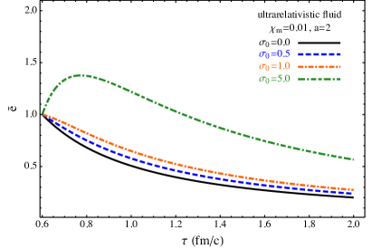
Figure 3: Left panel: the solutions (64), (65) for different values of the parameters. We choose $\chi_{m}=0.01$. The black solid line is for the case without magnetic field. For $\sigma_{0}=0.5$, the blue dashed, orange dash-dotted, and green dash-dotted lines are for $a=1/3,2/3,3/2$, respectively. Right panel: the same as in the left panel but for $\chi_{m}=0.01$ and $a=2$. The black solid line is for the case without magnetic fields. The blue dashed, orange dash-dotted, and green dash-dotted lines are for $\sigma_{0}=0.5,1.0,5.0$, respectively.

Since the term $\left[\left({\tau_{0}}/{\tau}\right)^{2a}-\left({\tau_{0}}/{\tau}\right)^{1+c_{s}^{2}}\right]/(1+c_{s}^{2}-2a)$ is always positive, from Eq. (64) we see that the effect of nonzero magnetization enters only through the prefactor $1-a-\chi_{m}$. More precisely, when $a>1-\chi_{m}$, $\tilde{e}$ decays more slowly than in the case without magnetic fields, and when $0<a<1-\chi_{m}$, $\tilde{e}$ decays faster. One can reach the same conclusion by analyzing the sign of the last term in Eq. (62). We can demonstrate our conclusion in two limits and, for simplicity, we assume $\chi_{m}>0$. For $a\rightarrow 0$, the magnetic field is constant in proper time and does not evolve with the fluid. Thus, the fluid energy density must decay faster in order to sustain this constant magnetic field. For $a\rightarrow\infty$, the magnetic field decays very rapidly and its energy will be transferred to the fluid due to the energy-conservation law. So, one can expect a peak of the energy density near the initial time, which is associated with a resistive “reheating” of the fluid Roy:2015kma .

We show these solutions in Fig. 3. Since $\chi_{m}$ is very small for the QGP, we choose a typical value $\chi_{m}=0.01$ in the left panel of Fig. 3. The black solid line is for the case without magnetic field, $\sigma_{0}=0$, while the blue dashed, orange dash-dotted, and green dash-dotted lines are for $a=1/3,2/3,3/2$, respectively, for the case $\sigma_{0}=0.5$. For $a>1-\chi_{m}$ the energy density decays more slowly and for $a<1-\chi_{m}$, it decays faster than without magnetization, respectively. In the right panel of Fig. 3, fixing $\chi_{m}=0.01$ and $a=2$, the blue dashed, orange dash-dotted, and green dash-dotted lines are for $\sigma_{0}=0.5,1.0,5.0$, respectively. If $\sigma_{0}$ is large enough, we can observe the initial “reheating” effect.

IV.2 Magnetized conformal fluid

We conclude this section by considering the evolution under external magnetic field (60) when the fluid obeys the EOS (35) for a magnetized conformal fluid. In this case, Eq. (62) becomes

$$\partial_{\tau}\tilde{e}+\frac{4}{3}\frac{\tilde{e}}{\tau}+\sigma_{0}\left(1-a-\frac{1}{3}\chi_{m}\right)\frac{\tau_{0}^{2a}}{\tau^{a+1}}=0\,.$$ (68)

The solution can be obtained similarly as above and reads

$$\tilde{e}(\tau)=\left(\frac{\tau_{0}}{\tau}\right)^{4/3}-\frac{\sigma_{0}}{2}\frac{3-3a-\chi_{m}}{2-3a}\left[\left(\frac{\tau_{0}}{\tau}\right)^{2a}-\left(\frac{\tau_{0}}{\tau}\right)^{4/3}\right]$$ (69)

for $a\neq 2/3$, and

$$\tilde{e}(\tau)=\left(\frac{\tau_{0}}{\tau}\right)^{4/3}+\frac{\sigma_{0}}{3}(1-\chi_{m})\left(\frac{\tau_{0}}{\tau}\right)^{4/3}\log\left(\frac{\tau_{0}}{\tau}\right)$$ (70)

for $a=2/3$. The normalized total energy density is

$$\hskip-11.38092pt\tilde{e}_{\rm tot}=\left(\frac{\tau_{0}}{\tau}\right)^{4/3}$$

$$\hskip 0.0pt+\frac{\sigma_{0}}{2}\left\{\left(\frac{\tau_{0}}{\tau}\right)^{2}-\frac{3-3a-\chi_{m}}{2-3a}\left[\left(\frac{\tau_{0}}{\tau}\right)^{2a}-\left(\frac{\tau_{0}}{\tau}\right)^{4/3}\right]\right\}$$

for $a\neq 2/3$, and

$$\tilde{e}_{\rm tot}=\left(\frac{\tau_{0}}{\tau}\right)^{4/3}+\frac{\sigma_{0}}{3}(1-\chi_{m})\left(\frac{\tau_{0}}{\tau}\right)^{4/3}\log\left(\frac{\tau_{0}}{\tau}\right)+\frac{\sigma_{0}}{2}\left(\frac{\tau_{0}}{\tau}\right)^{2}$$ (72)

for $a=2/3$. The behaviour of Eq. (69) can be discussed in a manner similar to the previous case of an ultrarelativistic fluid. When $a>1-\chi_{m}/3$, $\tilde{e}$ will decay more slowly than in the case without magnetic field, and when $0<a\leq 1-\chi_{m}/3$, $\tilde{e}$ will decay faster than in the case without magnetic field.

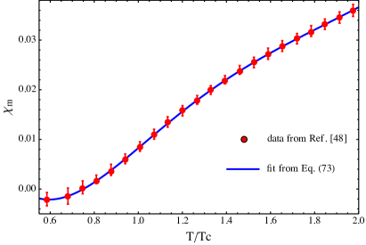
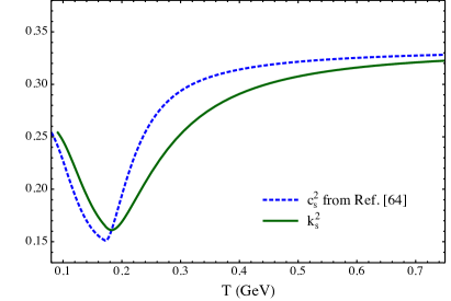
Figure 4: Left panel: magnetic susceptibility $\chi_{m}$; the filled red circles refer to the data in Ref. Bali:2014kia , while the solid line shows the fit given by Eq. (73). Right panel: behaviour of $k_{s}^{2}=p/e$ and of $c_{s}^{2}$. The dashed line shows the speed of sound given by Eq. (77) from the parametrization of Ref.  Huovinen:2009yb . Finally, the solid green line provides the ratio between the pressure and energy density; note the close similarity between $k_{s}^{2}$ and $c_{s}^{2}$.

V Energy-density evolution with temperature-dependent magnetic susceptibility

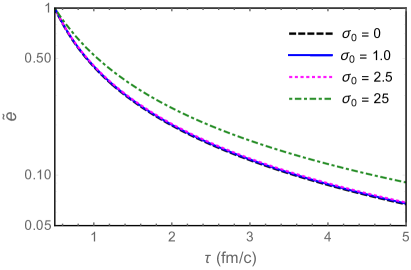
Figure 5: Evolution of temperature $T$ (left panel) and normalized energy density $\tilde{e}=e/e_{0}$ (right panel) as a functions of proper time $\tau$. We choose initial temperature $T_{0}=200$ MeV, initial time $\tau_{0}=0.5$ fm/c, and critical temperature $T_{c}=180$ MeV. The black dashed, blue solid, magenta dotted, and green dot-dashed lines are for $\sigma_{0}=0,1.0,2.5,25$, respectively.

After the rather academic discussion of the previous section, we will now consider a more realistic scenario. For the sake of simplicity, we will choose the temperature $T$ as independent variable and express all quantities as a function of $T$. We also choose the EOS named “s95n-v1” parametrization of Ref. Huovinen:2009yb , which is also obtained from lattice QCD Bazavov:2009zn . We will use lattice-QCD data for the magnetic susceptibility $\chi_{m}$ as a function of $T$ and investigate the effect of the magnetization across the deconfinement phase transition.

The behaviour of the magnetic susceptibility as a function of the temperature has been studied in lattice-QCD calculations following several different approaches [see, e.g., Refs. Kamikado:2014bua ; Bali:2014kia ; Bonati:2013vba ; Levkova:2013qda ]. Since we concentrate on the deconfinement phase transition and we expect that $\chi_{m}(T)$ becomes negative in the hadronic phase, we choose the data from Ref. Bali:2014kia . Noting that a power-law behaviour $(T/T_{c}-1)^{n}$ with $n={\rm const.}$ is typical for quantities near a phase transition, we capture the analytical behaviour of the data by expressing $\chi_{m}(T)$ as a polynomial in powers of $T/T_{c}-1$, i.e.,

$$\chi_{m}(T) = \sum_{n=0}c_{n}\left(\frac{T}{T_{c}}-1\right)^{n}\,,$$ (73)

where $T_{c}$ is the transition temperature and the first six coefficients appearing in Eq. (73) are given by $c_{0}=0.0082$, $c_{1}=0.0374$, $c_{2}=0.0039$, $c_{3}=-0.0427$, $c_{4}=0.0430$, and $c_{5}=-0.0138$.

Similarly, we introduce the parameter $k_{s}^{2}$, defined as

$$k_{s}^{2}(T)\equiv\frac{p}{e}\,,$$ (74)

which is a function of $T$. Note that $k_{s}^{2}$ is reminiscent of, but distinct from, the square of the sound speed $c^{2}_{s}$. The latter is in fact defined as in Eq. (29) and will in general be different from the simple ratio of the pressure and energy density [the only exception being the EOS of an ultrarelativistic fluid (34) or the EOS normally used in cosmology $p=we$ Rezzolla2013 ]. Hence, the parameter $k_{s}^{2}$ does not have a precise physical significance, but should be seen mostly as a mathematically convenient definition that allows us to express the pressure in terms of the energy density and hence obtain an analytic solution. Having said that, it is interesting also to remark that $k_{s}^{2}$ and $c^{2}_{s}$ are rather similar, as shown in the right panel of Fig. 4, where we compare our fitting functions for $\chi_{m}$ and $k_{s}^{2}$ with the original data from Refs. Bali:2014kia and Huovinen:2009yb .

From the “s95n-v1” parametrization of Ref. Huovinen:2009yb , $p(T)$ and $e(T)$ can be obtained by integrating over the temperature the trace anomaly $\theta(T)\equiv e(T)-3p(T)$

$$p(T)=T^{4}\int_{T_{1}}^{T}\frac{\theta(T^{\prime})}{T^{\prime 5}}dT^{\prime}\,,$$ (75)

where we choose $T_{1}=1\textrm{MeV}$ and the trace anomaly is given in Ref. Huovinen:2009yb

$$\theta(T)=T^{4}\begin{cases}{d_{2}}/{T^{2}}+{d_{4}}/{T^{4}}+{c_{1}}/{T^{n_{1}}}+{c_{2}}/{T^{n_{2}}},&T\geq T_{0},\\ a_{1}T+a_{2}T^{3}+a_{3}T^{4}+a_{4}T^{10},&T<T_{0}\,,\end{cases}$$ (76)

with $d_{2}=0.2654\,\textrm{GeV}^{2}$, $d_{4}=6.563\times 10^{-3}\,\textrm{GeV}^{4}$, $c_{1}=-4.370\times 10^{-5}\,\textrm{GeV}^{n_{1}}$, $c_{2}=5.774\times 10^{-6}\,\textrm{GeV}^{n_{2}}$, $n_{1}=8$, $n_{2}=9$, $T_{0}=171.8\,\textrm{MeV}$, $a_{1}=4.654\,\textrm{GeV}^{-1}$, $a_{2}=-879\,\textrm{GeV}^{-3}$, $a_{3}=8081\,\textrm{GeV}^{-4},$ $a_{4}=-7039000\,\textrm{GeV}^{-10}$. The ansatz in Eq. (76) parametrizes lattice-QCD data when $T\geq T_{0}$, while it it parametrizes data for a hadron resonance gas when $T<T_{0}$. Inserting Eqs. (75), (76) into Eq. (74), we can get an estimate of $k_{s}^{2}(T)$.

As shown in Fig. 4, we also obtain the (squared) speed of sound $c_{s}^{2}$ as a function of $T$ from the “s95n-v1” parametrization of Ref. Huovinen:2009yb ,

$$c_{s}^{2}=\frac{s}{T}\frac{dT}{ds},$$ (77)

where entropy density $s\equiv(4p+\theta)/T$ is computed from the trace anomaly and Eq. (75).

Since it is not trivial to obtain the energy density $e$ and the entropy density $s$ as functions of $T$, we will use the thermodynamical relation (28)

$$e=\frac{Ts}{1+k_{s}^{2}}=\frac{s_{0}\tau_{0}}{\tau}\frac{T}{1+k_{s}^{2}}\,,$$ (78)

where in the second equality we used the conservation of entropy. Inserting this into the differential equation (50), yields

$$\partial_{\tau}\left[\frac{T}{(1+k_{s}^{2})\tau}\right]+\frac{T}{\tau^{2}}-\frac{\tau_{0}}{\tau^{3}}\frac{T_{0}}{1+k_{s}^{2}(T_{0})}\sigma_{0}\chi_{m}=0\,.$$ (79)

After solving Eq. (79), we can simply obtain the energy density via

$$\tilde{e}\equiv\frac{e(\tau)}{e_{0}}=\frac{\tau_{0}}{\tau}\frac{T(\tau)}{T_{0}}\frac{1+k_{s}^{2}(T_{0})}{1+k_{s}^{2}(T(\tau))}\,.$$ (80)

Choosing the initial temperature $T_{0}$, the initial time $\tau_{0}$, and the critical temperature $T_{c}$ as

$$T_{0}=200\,{\rm MeV}\,,\quad T_{c}=180\,{\rm MeV}\,,\quad\tau_{0}=0.5\ {\rm fm/c}\,,$$ (81)

we solve Eq. (79) numerically and show the results in Fig. 5 for different $\sigma_{0}=0,1.0,2.5,25$, respectively. Note also that the decay of temperature and energy density is slowed down due to the magnetization effect. This is consistent with Eq. (79), which implies that the magnetic field becomes a source to reheat the system.

As a rough estimate, we can evaluate $\sigma_{0}$ in a typical Bjorken flow for the QGP. For 200 AGeV Au-Au collisions, the magnetic field can reach values of $B\sim 10\,m_{\pi}^{2}\sim 0.44$ GeV, while the energy density of the magnetic field will be $\frac{1}{2}B^{2}\sim 5$ GeV fm^-3. The initial energy density of the fluid $e_{0}$ will be $\sim 10$ GeV fm^-3. Thus we find $\sigma_{0}=B_{0}^{2}/e_{0}\simeq 0.5$, which is close the value for the blue solid lines in Fig. 5. Overall, this shows that for a Bjorken flow, the magnetization effect of the QGP can be ignored. On the other hand, for an ultra-large magnetic field, e.g., $\sigma_{0}=25$ which corresponds to $B\gtrsim 50\,m_{\pi}^{2}$, the temperature will increase, and then decrease, i.e., the system is first reheated by the magnetic field. In that case, which is similar to the one shown in Fig. 3, the QGP can survive longer than otherwise expected.

VI Conclusion

We have studied the evolution of the energy density of the QGP produced, for instance, by the collision of two heavy ions, when this is described as a one-dimensional, longitudinally boost-invariant flow with a transverse magnetic field, i.e., a transverse Bjorken flow within the ideal-MHD limit. This represents a rather straightforward extension of our previous work Roy:2015kma to the case in which the flow has a nonzero magnetization as described via a magnetic susceptibility $\chi_{m}$, which we have taken to be either constant or to depend on temperature.

Under these conditions for the Bjorken flow, we were able to obtain analytic solutions relative to two different EOSs, i.e., the EOS (34) for an ultrarelativistic fluid and the EOS (35) for a magnetized conformal fluid. Interestingly, we find that all results for a magnetized conformal fluid can be obtained from the solutions for an ultrarelativistic fluid after a simple scaling of the susceptibility, i.e., by replacing $\chi_{m}\rightarrow\chi_{m}/3$. We also find that for a paramagnetic fluid, i.e., with $\chi_{m}>0$, the fluid gains energy from the decay of the magnetic field, thus with an energy density decaying more slowly than in the case without magnetic fields. On the other hand, for a diamagnetic fluid, i.e., with $\chi_{m}<0$, the fluid loses energy to the magnetic field and the energy density will decay more rapidly than in the absence of a magnetic field.

We have also considered the case where the magnetic field is external and very large, with an evolution that follows a power-law behaviour in proper time with exponent $a$. The solutions in this case can be distinguished in terms of two scenarios. The magnetic field decays more slowly than in the ideal-MHD case for $a>1-\chi_{m}$, while the decay is more rapid for $a<1-\chi_{m}$.

If the magnetic field or, strictly speaking, $\sigma_{0}=B_{0}^{2}/e_{0}$, is large enough, the fluid will absorb energy in excess of the decay caused by the expansion. In that case, one will observe a peak in the energy density at the early stage. This is a resistive “reheating” of the fluid. The amount of this increase depends on the magnetic-field strength and hence will increase with $\sigma_{0}$ and $a$. However, at late times, its energy density will decrease with an asymptotic rate that is the same as in the Bjorken flow, i.e., $\propto\tau^{-4/3}$.

Finally, we have also considered a temperature-dependent magnetic susceptibility and a realistic equation of state given by lattice-QCD data. We find that the magnetization effect of the QGP will slow down the decay of temperature and energy density. However, for realistic values of the magnetic susceptibility and initial magnetic field, this effect can be ignored, at least in a one-dimensional Bjorken flow. For an ultra-large magnetic field, on the other hand, the system might be reheated and the QGP may survive longer than expected.

- (1) A. Bzdak and V. Skokov, Phys.Lett. B710, 171 (2012), 1111.1949.
- (2) W.-T. Deng and X.-G. Huang, Phys.Rev. C85, 044907 (2012), 1201.5108.
- (3) H. Li, X.-l. Sheng, and Q. Wang, (2016), 1602.02223.
- (4) M. Gyulassy and L. McLerran, Nucl. Phys. A750, 30 (2005), nucl-th/0405013.
- (5) D. E. Kharzeev, L. D. McLerran, and H. J. Warringa, Nucl.Phys. A803, 227 (2008), 0711.0950.
- (6) K. Fukushima, D. E. Kharzeev, and H. J. Warringa, Phys.Rev. D78, 074033 (2008), 0808.3382.
- (7) D. E. Kharzeev and H.-U. Yee, Phys.Rev. D83, 085007 (2011), 1012.6026.
- (8) Y. Burnier, D. E. Kharzeev, J. Liao, and H.-U. Yee, Phys.Rev.Lett. 107, 052303 (2011), 1103.1307.
- (9) M. Stephanov and Y. Yin, Phys.Rev.Lett. 109, 162001 (2012), 1207.0747.
- (10) J.-W. Chen, J.-y. Pang, S. Pu, and Q. Wang, Phys.Rev. D89, 094003 (2014), 1312.2032.
- (11) J.-Y. Chen, D. T. Son, M. A. Stephanov, H.-U. Yee, and Y. Yin, Phys.Rev.Lett. 113, 182302 (2014), 1404.5963.
- (12) D. T. Son and N. Yamamoto, Phys.Rev.Lett. 109, 181602 (2012), 1203.2697.
- (13) D. T. Son and N. Yamamoto, Phys.Rev. D87, 085016 (2013), 1210.8158.
- (14) J.-H. Gao, Z.-T. Liang, S. Pu, Q. Wang, and X.-N. Wang, Phys.Rev.Lett. 109, 232301 (2012), 1203.0725.
- (15) J.-W. Chen, S. Pu, Q. Wang, and X.-N. Wang, Phys.Rev.Lett. 110, 262301 (2013), 1210.8312.
- (16) A. Bzdak, V. Koch, and J. Liao, Lect.Notes Phys. 871, 503 (2013), 1207.7327.
- (17) D. E. Kharzeev, Prog.Part.Nucl.Phys. 75, 133 (2014), 1312.3348.
- (18) D. E. Kharzeev, (2015), 1501.01336.
- (19) R.-H. Fang, J.-H. Gao, S. Pu, and Q. Wang, Chiral kinetic theory and berry phase from quantum kinetic approaches, in preparation.
- (20) X.-G. Huang and J. Liao, Phys.Rev.Lett. 110, 232302 (2013), 1303.7192.
- (21) S. Pu, S.-Y. Wu, and D.-L. Yang, Phys.Rev. D89, 085024 (2014), 1401.6972.
- (22) Y. Jiang, X.-G. Huang, and J. Liao, Phys.Rev. D91, 045001 (2015), 1409.6395.
- (23) S. Pu, S.-Y. Wu, and D.-L. Yang, Phys.Rev. D91, 025011 (2015), 1407.3168.
- (24) P. Romatschke and U. Romatschke, Phys. Rev. Lett. 99, 172301 (2007), 0706.1522.
- (25) M. Luzum and P. Romatschke, Phys. Rev. C78, 034915 (2008), 0804.4015.
- (26) H. Song and U. W. Heinz, Phys.Lett. B658, 279 (2008), 0709.0742.
- (27) H. Song and U. W. Heinz, Phys. Rev. C78, 024902 (2008), 0805.1756.
- (28) B. Schenke, S. Jeon, and C. Gale, Phys. Rev. C85, 024901 (2012), 1109.6289.
- (29) V. Roy, A. K. Chaudhuri, and B. Mohanty, Phys. Rev. C86, 014902 (2012), 1204.2347.
- (30) H. Niemi, G. S. Denicol, P. Huovinen, E. Molnar, and D. H. Rischke, Phys. Rev. C86, 014909 (2012), 1203.2452.
- (31) L. Rezzolla and O. Zanotti, Relativistic Hydrodynamics (Oxford University Press, 2013).
- (32) U. Gursoy, D. Kharzeev, and K. Rajagopal, Phys. Rev. C89, 054905 (2014), 1401.3805.
- (33) B. G. Zakharov, Phys. Lett. B737, 262 (2014), 1404.5047.
- (34) K. Tuchin, Phys.Rev. C88, 024911 (2013), 1305.5806.
- (35) V. Roy, S. Pu, L. Rezzolla, and D. Rischke, (2015), 1506.06620.
- (36) V. Roy and S. Pu, (2015), 1508.03761.
- (37) J. D. Bjorken, Phys. Rev. D27, 140 (1983).
- (38) L. Landau and E. M. Lifshitz, Fluid dynamics (Pergamon, New York, 1959).
- (39) G. S. Bali, F. Bruckmann, G. Endrodi, and A. Schafer, Phys. Rev. Lett. 112, 042301 (2014), 1311.2559.
- (40) B. L. Ioffe and A. V. Smilga, Nucl. Phys. B232, 109 (1984).
- (41) G. S. Bali et al., Phys. Rev. D86, 094512 (2012), 1209.6015.
- (42) P. V. Buividovich, M. N. Chernodub, E. V. Luschevskaya, and M. I. Polikarpov, Nucl. Phys. B826, 313 (2010), 0906.0488.
- (43) M. Frasca and M. Ruggieri, Phys. Rev. D83, 094024 (2011), 1103.1194.
- (44) C. Bonati, M. D’Elia, M. Mariti, F. Negro, and F. Sanfilippo, Phys.Rev.Lett. 111, 182001 (2013), 1307.8063.
- (45) C. Bonati, M. D’Elia, M. Mariti, F. Negro, and F. Sanfilippo, PoS LATTICE2013, 184 (2014), 1312.5070.
- (46) L. Levkova and C. DeTar, Phys. Rev. Lett. 112, 012002 (2014), 1309.1142.
- (47) C. Bonati, M. D’Elia, M. Mariti, F. Negro, and F. Sanfilippo, Phys. Rev. D89, 054506 (2014), 1310.8656.
- (48) Yu. A. Simonov and V. D. Orlovsky, JETP Lett. 101, 423 (2015), 1405.2697.
- (49) G. S. Bali, F. Bruckmann, G. Endrodi, S. D. Katz, and A. Schafer, JHEP 08, 177 (2014), 1406.0269.
- (50) K. Kamikado and T. Kanazawa, JHEP 01(2015)129, 01129 (2014), 1410.6253.
- (51) O. Bergman, G. Lifschytz, and M. Lippert, JHEP 05, 007 (2008), 0802.3720.
- (52) A. Cherman, T. D. Cohen, and E. S. Werbos, Phys. Rev. C79, 045203 (2009), 0804.1096.
- (53) T. Steinert and W. Cassing, Phys. Rev. C89, 035203 (2014), 1312.3189.
- (54) D. N. Kabat, K.-M. Lee, and E. J. Weinberg, Phys. Rev. D66, 014004 (2002), hep-ph/0204120.
- (55) M. M. Anber and M. Unsal, JHEP 12, 107 (2014), 1309.4394.
- (56) A. N. Tawfik and N. Magdy, Phys. Rev. C90, 015204 (2014), 1406.7488.
- (57) M. M. Caldarelli, O. J. C. Dias, and D. Klemm, JHEP 03, 025 (2009), 0812.0801.
- (58) M. Gedalin and I. Oiberman, Phys. Rev. E 51, 4901 (1995).
- (59) X.-G. Huang, M. Huang, D. H. Rischke, and A. Sedrakian, Phys. Rev. D81, 045015 (2010), 0910.3633.
- (60) S. R. de Groot, The Maxwell equations :non-relativistic and relativistic derivations from electron theory (North-Holland Pub. Co, 1969).
- (61) B. Giacomazzo and L. Rezzolla, J. Fluid Mech. 562, 223 (2006), gr-qc/0507102.
- (62) B. Giacomazzo and L. Rezzolla, Class. Quant. Grav. 24, S235 (2007), gr-qc/0701109.
- (63) L. Landau, E. Lifshitz, and L. Pitaevskii, Electrodynamics of continuous media. Course of theoretical physics (Butterworth-Heinemann, Oxford U.K., 1995).
- (64) G. Bali, F. Bruckmann, G. Endrodi, F. Gruber, and A. Schaefer, JHEP 1304, 130 (2013), 1303.1328.
- (65) P. Huovinen and P. Petreczky, Nucl. Phys. A837, 26 (2010), 0912.2541.
- (66) A. Bazavov et al., Phys. Rev. D80, 014504 (2009), 0903.4379.
- (67) L.-g. Pang, G. Endrodi, G.di, and H. Petersen, (2016), 1602.06176.