Effects of a dressed quark-gluon vertex in vector heavy-light mesons
and theory average of $B_{c}^{*}$ meson mass

Abstract

We extend earlier investigations of heavy-light pseudoscalar mesons to the vector case, using a simple model in the context of the Dyson-Schwinger-Bethe-Salpeter approach. We investigate the effects of a dressed-quark-gluon vertex in a systematic fashion and illustrate and attempt to quantify corrections beyond the phenomenologically very useful and successful rainbow-ladder truncation. In particular we investigate dressed quark photon vertex in such a setup and make a prediction for the experimentally as yet unknown mass of the $B_{c}^{*}$, which we obtain at $6.334$ GeV well in line with predictions from other approaches. Furthermore, we combine a comprehensive set of results from the theory literature. The theory average for the mass of the $B_{c}^{*}$ meson is $6.336\pm 0.002$ GeV.

I Introduction

The Dyson-Schwinger-Bethe-Salpeter-equation (DSBSE) approach is a modern nonperturbative framework based on continuum quantum field theory Roberts et al. (2007); Fischer (2006); Alkofer and von Smekal (2001); Sanchis-Alepuz and Williams (2015a) and is thus complementary to lattice-regularized QCD Dudek et al. (2008); Lang et al. (2011); Liu et al. (2012); Thomas (2013); Flynn et al. (2015); Lang et al. (2015) and other modern approaches to the strong-interaction sector of the standard model of elementary particle physics.

Modern DSBSE studies with phenomenological background mostly use a setup where a simple truncation is combined with a sophisticated effective model interaction, see Maris and Tandy (1999); Holl et al. (2003, 2004); Krassnigg and Maris (2005); Holl et al. (2005a); Alkofer et al. (2006); Eichmann et al. (2008a, 2009, b); Krassnigg (2009); Eichmann et al. (2010); Alkofer et al. (2010); Krassnigg and Blank (2011); Dorkin et al. (2011); Blank and Krassnigg (2010); Blank et al. (2011); Mader et al. (2011); Blank and Krassnigg (2011a); Hilger (2012); Popovici et al. (2015); Hilger et al. (2015a); Fischer et al. (2014, 2015); Hilger et al. (2015b, c); Hilger (2015); Raya et al. (2015) and references therein. Beyond the most popular rainbow-ladder (RL) truncation, systematic schemes exist to explore the infinite system of Dyson-Schwinger equations (DSEs) in a symmetry-preserving fashion Bender et al. (1996); Sanchis-Alepuz and Williams (2015a). In a concrete, numerical setup Bhagwat et al. (2007a); Krassnigg (2008); Blank and Krassnigg (2011b, c); Blank (2011), one faces increasing complexity Watson and Cassing (2004); Watson et al. (2004); Fischer et al. (2005); Fischer and Williams (2008, 2009); Williams (2010, 2015); Sanchis-Alepuz et al. (2014); Chang and Roberts (2009); Heupel et al. (2014); Sanchis-Alepuz and Williams (2015b); Williams et al. (2015); Fu and Wang (2016); Binosi et al. (2016); Qin (2016) such that simple models are of an obvious advantage, e. g., Horvatic et al. (2007, 2008, 2011); Roberts et al. (2011); Gutierrez-Guerrero et al. (2010); Bedolla et al. (2015); Segovia (2016) and references therein.

A particularly simple effective interaction Munczek and Nemirovsky (1983) is also employed in our present work, which was used in the past to study certain classes of diagrams or particular effects of interest Bender et al. (1996); Alkofer and von Smekal (2001); Bender et al. (2002); Krassnigg and Roberts (2004); Bhagwat et al. (2004); Holl et al. (2005b); Matevosyan et al. (2007a, b); Jinno et al. (2015). These can then easily serve as both a testing ground for and a means to estimate missing effects in a setup using a more sophisticated effective interaction.

In this work we continue an investigation of a systematically dressed quark-gluon vertex (QGV) which consistently enters both the quark DSE and the meson Bethe-Salpeter-equation (BSE) via their respective integral-equation kernels Bender et al. (2002); Bhagwat et al. (2004); Gomez-Rocha et al. (2015a, b). Following up on Gomez-Rocha et al. (2015b), our focus remains on heavy-light mesons, which probe the underlying equations and their building blocks such as the QGV in different ways. For example, dressing effects for the quark propagator have been questioned and tested for the case of b-quarks Nguyen et al. (2009); Souchlas and Stratakis (2010); Nguyen et al. (2011), since one can make use of simplifying assymptions about the heavy-quark propagator based on the large value of the quark mass Ivanov et al. (1998a, b, 1999); Blaschke et al. (2000); Bhagwat et al. (2007b); Ivanov et al. (2007); El-Bennich et al. (2010, 2011). Ultimately, one goal is to check heavy-quark symmetry predictions Neubert (1994) as, e. g., in relativistic Hamiltonian dynamics Keister and Polyzou (1991); Krassnigg et al. (2003); Krassnigg (2005); Polyzou (2015) as well as reduced versions of the BSE Blankenbecler and Sugar (1966); Gross (1969), where heavy quarks have been under renewed investigation recently Gomez-Rocha and Schweiger (2012); Gomez-Rocha (2014); Li et al. (2015); Leitão et al. (2015). Another goal is to prepare, e. g., investigations of the spectral difference of parity partners in analogy to recent progress with QCD sum rules Thomas et al. (2008); Hilger and Kämpfer (2009); Hilger et al. (2010, 2012a, 2011, 2012b); Buchheim et al. (2015a); Gubler and Ohtani (2014); Buchheim et al. (2015b, c); Gubler and Weise (2015).

The article is organized as follows: In Sec. II we briefly sketch the setup used for the quark DSE, the QGV, and the meson BSE. Results and discussion are presented in Sec. III; conclusions follow in Sec. IV. Technical details are collected in the appendices.

II Setup

Since this work is an extension of Bender et al. (2002); Bhagwat et al. (2004); Gomez-Rocha et al. (2015b), we only very briefly sketch the relevant formulae, mostly in order to be able to understand and interpret the results presented as well as to connect to the new details presented in the appendices. For a more complete presentation of our particular setup and approach, see Gomez-Rocha et al. (2015b). More details on the case of equal-mass constituents can be found in Bhagwat et al. (2004), and the truncation scheme and basic assumptions are laid out in Bender et al. (2002). Our calculations are performed in Euclidean momentum space.

II.1 Quark DSE

Solution of a bound-state problem in the DSBSE formalism requires knowledge of the building blocks and their interactions. In our case the meson BSE requires us to know the quark propagator for both the heavy and the light quark under consideration, and the quark-gluon interaction as well as the gluon propagator. We go in medias res by assuming the simplification inherent in the effective interaction of Munczek and Nemirovsky (1983), namely the Munczek-Nemirovsky (MN) gluon-momentum dependence

$$D_{\mu\nu}(k)\sim\mathcal{G}^{2}\,\delta^{4}(k)\,,$$ (1)

where $D_{\mu\nu}$ is the renormalized dressed gluon propagator and $\mathcal{G}$ an effective coupling constant, which sets the scale of the model. This transforms all integral equations into algebraic equations. In addition, since this model is UV finite, all renormalization constants are $=1$.

In particular, the quark DSE reads

$$S^{-1}(p)=i\gamma\cdot p+m_{q}+\gamma_{\mu}S(p)\Gamma_{\mu}^{\mathcal{C}}(p)\;,$$ (2)

where the renormalized dressed quark propagator $S$ has the form

$$S(p)^{-1} = i\gamma\cdot pA(p^{2})+B(p^{2})$$ (3)

$$= A(p^{2})\left(i\gamma\cdot p+M(p^{2})\right)\;$$ (4)

with the dressing functions $A$ and $B$ or, alternatively, $A$ and $M$; $m_{q}$ is the current-quark mass, and flavor is inherent to the solution depending on $m_{q}$.

The renormalized dressed QGV is written as $\Gamma^{a}_{\nu}$ with the color index ^a, which we write explicitly as $\Gamma_{\mu}^{a}(p)=\frac{\lambda^{a}}{2}\Gamma_{\mu}(p)$. Furthermore, we have set $\mathcal{G}=1$ in Eq. (2) and the following, thereby obtaining all dimensioned quantities in appropriate units of $\mathcal{G}$. The model parameter $\mathcal{C}$ introduced in Eq. (2) and its meaning are best illustrated via the DSE for the QGV, following Bhagwat et al. (2004) obtained as the effective equation

$$\Gamma_{\mu}^{\mathcal{C}}(p)=\gamma_{\mu}-\mathcal{C}\,\gamma_{\rho}\,S(p)\,\Gamma_{\mu}^{\mathcal{C}}(p)\,S(p)\,\gamma_{\rho}\;,$$ (5)

where the dependence on $\mathcal{C}$ stems from the effective combination of the abelian and non-abelian correction terms in the QGV DSE, and the value of $\mathcal{C}$ is chosen in accordance with, e. g., lattice QCD or phenomenology.

Concrete possible values are: $\mathcal{C}=-1/8$, corresponding to abelian-only dressing Bender et al. (2002); $\mathcal{C}=0$ corresponding to RL truncation; $\mathcal{C}=0.51$, used in Bhagwat et al. (2004) as a result from fitting to lattice quark propagators Bowman et al. (2003, 2002); Bhagwat et al. (2003). Herein, we fix $\mathcal{C}=0.51$ throughout for easy comparison and direct connection to the earlier studies of Bhagwat et al. (2004); Gomez-Rocha et al. (2015b).

To define our truncation scheme Bender et al. (2002), we iterate eq. (5) such that the bare QGV serves as a starting value $\Gamma_{\mu,0}^{\mathcal{C}}(p)=\gamma_{\mu}$ and the recursion relation is

$$\Gamma_{\mu,i}^{\mathcal{C}}(p)=-\mathcal{C}\,\gamma_{\rho}\,S(p)\,\Gamma_{\mu,i-1}^{\mathcal{C}}(p)\,S(p)\,\gamma_{\rho}\;.$$ (6)

At a given order $n$ in this scheme one has for the QGV

$$\Gamma_{\mu}^{\mathcal{C}}(p)=\sum_{i=0}^{n}\Gamma_{\mu,i}^{\mathcal{C}}(p).$$ (7)

and the fully dressed result for the QGV is obtained by $n\rightarrow\infty$. Note that the flavor content of Eqs. (5) and (6) is implicitly carried by the factors of $S$.

II.2 Meson BSE

The meson BSE in the current setup is simplified in a similar fashion to the quark DSE, namely via the effective interaction’s property (1). The solution of the BSE, the Bethe-Salpeter amplitude (BSA) is often combined with the quark propagators in the integration kernel to the so-called Bethe-Salpeter wave function $\chi$ and we have

$$\chi(P):=S(q_{+})\,\Gamma(P)\,S(q_{-})\;.$$ (8)

The meson flavor is determined by the quark flavors of the two factors of $S$, and the total meson momentum is the only remaining variable, since the quark and antiquark momenta are reduced to $q_{+}=\eta P$ and $q_{-}=-(1-\eta)P$.

The momentum partitioning parameter $\eta\in[0,1]$ is in principle arbitrary in any covariant computation as a result of the freedom in the definition of the quark-antiquark relative momentum such that observables are independent of $\eta$. However, our particular model interaction is oversimplifying in the sense that not all possible covariant structures of the BSA are retained. As a result, there is a dependence on $\eta$, which is a model artifact and must be properly analyzed in any study using this particular interaction. Such an analysis was already performed in Ref. Munczek and Nemirovsky (1983) and also in our previous work on pseudoscalar mesons in Gomez-Rocha et al. (2015b); for our present study, this analysis is presented in App. A. In the presence of such a detailed analysis, this model artifact does not destroy the model’s capacity to elucidate our investigation’s goals. Furthermore, it is easily quantified and thus well under control.

For the unequal-mass case in our setup, the BSE reads, see Gomez-Rocha et al. (2015b) and App. C,

$$\Gamma^{M}(P) = -\frac{1}{2}\left[\gamma_{\mu}\chi^{M}(P)\,\Gamma_{\mu}^{\mathcal{C}}(q_{-})\right.$$ (9)

$$+ \gamma_{\mu}S(q_{+})\,\Lambda^{M}_{\mu}(P)+\Gamma_{\mu}^{\mathcal{C}}(q_{+})\chi^{M}(P)\gamma_{\mu}$$

$$+ \left.\Lambda^{M}_{\mu}(P)S(q_{-})\gamma_{\mu}\right]\;.$$

The superscript label ^M denotes the type of meson under study, since the structure of the correction term $\Lambda^{M}_{\mu}$ depends on the structure of the corresponding BSA. Herein we consider the vector meson case, for which all details are given appropriately in the appendices.

The quark momenta $q_{\pm}$ in this equation denote the flavor content and, in particular, the mass ordering among the quarks in that the heavier quark is associated with the subscript ₊.

While the first term on the r.h.s. of Eq. (9) is straight-forward to construct from a given QGV, the construction of the second term is based on a recursion relation analogous to the one for the QGV. Correction terms are summed up to a particular order $n$ to get $\Lambda^{M}$ as

$$\Lambda^{M}_{\nu}(P)=\sum_{i=0}^{n}\Lambda_{\nu,i}^{M}(P)\,,$$ (10)

and the full result is then obtained by $n\rightarrow\infty$.

The recursion relation reads Bender et al. (2002); Bhagwat et al. (2004):

$$\frac{1}{\mathcal{C}}\Lambda_{\nu,n}^{M}(P) = -\gamma_{\rho}\chi^{M}(P)\Gamma_{\nu,n-1}^{\mathcal{C}}(q_{-})S(q_{-})\gamma_{\rho}$$ (11)

$$- \gamma_{\rho}S(q_{+})\Gamma_{\nu,n-1}^{\mathcal{C}}(q_{+})\chi^{M}(P)\gamma_{\rho}$$

$$- \gamma_{\rho}S(q_{+})\Lambda_{\nu,n-1}^{M}(P)S(q_{-})\gamma_{\rho}\;,$$

where quark flavors and properties in the factors of $S$ and $\Gamma_{\nu}$ are given via the subscripts _± in their argument, as described above.

Evaluating the recursion relations to a desired order, one uses the initial condition Bender et al. (2002)

$$\Lambda_{\nu,0}^{M}(P)=0\;.$$ (12)

In the pseudoscalar case for equal-mass quarks and $\eta=1/2$ this implies Bender et al. (2002)

$$\Lambda_{\nu,0}^{\mathrm{P}}(P)=0\quad\Rightarrow\quad\Lambda_{\nu}^{\mathrm{P}}(P)\equiv 0\;,$$ (13)

which was used as a testing case for our general setup in Gomez-Rocha et al. (2015b). In the vector case, however, no symmetry exists to enable such a cancellation and thus an appropriate testing case is the equal-mass result presented in Bender et al. (2002). Further details on the construction of $\Lambda_{\nu}^{\mathrm{V}}(P)$ are technical and thus collected in App. B.

III Results and Discussion

We investigate the effect of QGV dressing on vector-meson ground-state masses in the scheme described above as a representative way to apply systematic corrections to the often and well used RL truncation.

As mentioned above, our simplified model leads to an artificial dependence on the momentum-partitioning parameter $\eta$, which one must study, but nontheless not put in the center of attention. We present the dependence on $\eta$ in detail in App. A and produce corresponding error bars in our comparison to experimental data below in Fig. 1; however, other than this we focus on one particular representative value for $\eta$ and compare our results for the various dressing stages in the scheme in physically meaningful ways.

The study of mesons with unequal-mass constituents was started in Ref. Gomez-Rocha et al. (2015b) for the pseudoscalar case. While we presented also some detailed analysis of the quark propagator dressing functions there, we will not repeat those here. Instead, our focus is the vector-meson case in general and two interesting items in particular: First, we study the dressed quark-photon vertex by solving the inhomogeneous BSE for the first time in the scheme under consideration here. Second, we predict the mass of the $B_{c}^{*}$ meson via a pseudoscalar-vector-splitting analysis. Overall, our results allow not only qualitative, but also quantitative statements.

Our model parameters are fixed to the values used earlier in Bhagwat et al. (2004) and Gomez-Rocha et al. (2015b): $\mathcal{C}=0.51$, $\mathcal{G}=0.69$, and the current-quark masses are $m_{u}=0.01$ GeV, $m_{s}=0.166$ GeV, $m_{c}=1.33$ GeV, $m_{b}=4.62$ GeV. For the light isovector case we assume isospin symmetry and the equality of the current-quark masses of the $u$ and $d$ quarks.

Note that this set of parameters was originally found to fit quarkonium vector-meson masses throughout the entire quark-mass range. As a result, our numbers presented below in Fig. 1 are not aimed at nor to be understood in the sense of a pure theory-experiment comparison. While in some cases agreement is excellent and the use of splittings is a perfectly fine example of a valid technique under our circumstances, we would like to stress the emphasis on the size of dressing effects as they are produced here.

III.1 Meson BSE

We present results for vector-meson ground-state masses. In the figures in this section, we plot meson masses as functions of the order $n$ in our truncation scheme. In addition, we discuss the differences of the various masses from the fully dressed result at every $n$ below. Before we discuss the results and figures in detail, we remark that it is possible that the homogeneous BSE doesn’t have a solution for a particular setup, configuration or set of parameters. In such a case the corresponding data point’s place in the figure is left empty.

Figure 1: Bound-state masses for $\rho$ meson, $\varphi$, $J/\Psi$, $\Upsilon$, and all different flavored vector ground states as a function of $n$, given in GeV. The dependence on $\eta$ is illustrated via the error bars. Calculated results are given by blue dots; experimental data are represented by horizontal lines. Olive and others (Particle Data Group)

Let us look at the convergence of the results with $n$ and the comparison with experimental data first. These results are presented in Fig. 1 in several boxes, one for each quark-flavor combination. The filled circles in the plots are our results for each $n$, where available, for a fixed value of $\eta$ in each case. In particular: $\eta=0.5$ for the $\rho$, $\varphi$, $J/\Psi$, and $\Upsilon$, $0.6$ for the $K^{*}$, $0.75$ for the $B_{c}^{*}$, $0.8$ for the $D^{*}$ and $D_{s}^{*}$, $0.9$ for the $B_{s}^{*}$, and $0.95$ for the $B^{*}$.

The actual $\eta$ dependence for each case is encoded in the form of a systematic error in our results in Fig. 1: the error bars are plotted from the lowest to the largest value of the mass result for any given $n$. Thus, they are asymmetric and the value of $\eta$ chosen for the data point, as defined below, can be also either the smallest or the largest value available at this $n$.

It should be noted here that we chose each $\eta$ via the requirement to find a solution of the BSE for all $n$, if possible. While this doesn’t seem to work for odd values of $n$, we are able to find $\eta$ values such that a solution can be obtained for $n=\infty$ in addition to the even values of $n$. As it turns out (see also the figures in App. A) this corresponds to a value of $\eta$ where the dressing effects for the meson under consideration are close to minimal with respect to their range as functions of $\eta$. The asymmetric values given above also make sense in correlation to the asymmetry of the quark-antiquark-mass content in each meson. The various aspects of $\eta$ and their influence on the quark-propagator dressing functions have been discussed in detail in our previous investigation for the pseudoscalar meson-case in Ref. Gomez-Rocha et al. (2015b). One may, at this point, speculate that an actual minimization of the dressing effects over the $\eta$-parameters space would lead to values very similar to the ones quoted here.

The largest error bars resulting from the $\eta$ range appear to be of the order of 20%, which is in rough agreement with our previous work Gomez-Rocha et al. (2015b) as well as the analysis in the original Munczek and Nemirovsky (1983), where the authors quote changes smaller than 15%. However, our detailed analysis presented in the plots in Figs. 6 and 7 in App. A clearly indicate that the extreme values $\eta=0$ and $1$ produce those masses with the largest deviations from the data point chosen for experimental comparison. In contrast to the observation regarding close-to-minimal dressing effects for our chosen values of $\eta$, one could state here that at the boundaries of the $\eta$ interval $[0,1]$ dressing effects appear to be maximal instead. This effect can also be traced back to the extended domain probed by extreme $\eta$ values in the quark-propagator dressing functions that are involved via the quark momenta squared $q_{\pm}^{2}$, which are directly proportional to $\eta^{2}$ and $(1-\eta)^{2}$, respectively. It is on these extended domains that dressing effects are larger than close to or in the spacelike domain Gomez-Rocha et al. (2015b).

In this sense it is certainly correct to state that the error bars in Fig. 1 should represent the entire range of $\eta$ observed in our calculations; on the other hand it also means that in practice the extreme $\eta$ values have to be taken with a grain of salt in the sense that they may not be representative to an amount that actually justifies the size of these error bars and we in general regard them as overestimates of more suitably defined systematic errors. In addition, we remark that the figures in App. A also show cases where very few or even only one of the $\eta$ values on our standard grid produce a solution of the corresponding BSE. These cases are easily recognized by their small error bars, which we chose not to rescale or blow up artificially. Note that it is possible that solutions exist for values of $\eta$ that are not part of our standard grid.

In terms of the comparison to experiment and the convergence behavior we find a clear pattern of higher, even $n$ lowering the meson mass with the fully dressed result again being lower than the result for our largest finite $n$ presented here, namely $n=4$. For odd $n$ in general no solutions were found. We note at this point why we do not find solutions in the odd-$n$ cases: our solutions of the homogeneous BSE are obtained by finding zeros of the appropriate determinant. It turns out that for the odd-$n$ cases, the determinant becomes complex at and below some particular negative value for $P^{2}$. If a zero is found above this value (which is the case for some of the pseudoscalar cases studied in Gomez-Rocha et al. (2015b)), we have a solution. For the present investigation of vector-mesons, which are heavier than their pseudoscalar counterparts, it appears that no zero of the determinant exists on the domain where it is still real.

Experimental values for the quarkonia were fitted via the quark masses, which is evident from the corresponding subplots in Fig. 1. For the $K^{*}$, agreement of the fully dressed result and the experimental mass value is excellent; in the other cases, experimental values are underestimated by our results. An experimental value for the mass of the $B_{c}^{*}$ meson is still missing, and we predict a value below via the use of the pseudoscalar-vector mass splitting.

Figure 2: Relative mass differences $\Delta m_{H}^{\mathrm{rel}\,n}$ to fully dressed result for $\rho$ meson, $\varphi$, $J/\Psi$, $\Upsilon$, and all different flavored vector ground states as a function of $n$ analogous to Fig. 1. Note that by definition Eq. (14) one obtains $\Delta m_{H}^{\mathrm{rel}\,\infty}=0$ in each case.

Next we have a look at the relative differences of meson masses at each value of $n$ compared to $n=\infty$, defined via

$$\Delta m_{H}^{\mathrm{rel}\,n}:=\frac{\Delta m_{H}^{n}}{m_{H}^{n\rightarrow\infty}}:=\frac{m_{H}^{n}-m_{H}^{n\rightarrow\infty}}{m_{H}^{n\rightarrow\infty}}\;,$$ (14)

which is dimensionless. Note that instead of comparing the difference to the fully dressed result here, one may also divide by the RL result; however, such a construction is uniquely related to Eq. (14) and, since the differences are small, this choice does not affect our discussion.

Table 1: Absolute and relative mass differences for the vector mesons with all possible flavor combinations, together with the corresponding pseudoscalar values adapted from Ref. Gomez-Rocha et al. (2015b). $\Delta m_{H}^{0}$ is given in GeV, the other quantities are dimensionless (see text).

$H$	$\Delta m_{H}^{0}$	$\Delta m_{H}^{\mathrm{rel}\,0}$	$\Delta m_{H}^{0}(\mathrm{P})$ Gomez-Rocha et al. (2015b)	$\Delta m_{H}^{\mathrm{rel}\,0}(\mathrm{P})$ Gomez-Rocha et al. (2015b)
$\rho$	0.226	0.294	0.011	0.078
$\varphi$	0.208	0.204	…	…
$J/\Psi$	0.105	0.034	0.048	0.016
$\Upsilon$	0.027	0.003	0.016	0.002
$K^{*}$	0.224	0.250	0.031	0.072
$D^{*}$	0.205	0.106	0.059	0.034
$B^{*}$	0.346	0.068	0.124	0.025
$D_{s}^{*}$	0.237	0.116	0.074	0.039
$B_{s}^{*}$	0.171	0.033	0.099	0.019
$B_{c}^{*}$	0.122	0.020	0.150	0.024

The results for $\Delta m_{H}^{\mathrm{rel}\,n}$ are plotted Fig. 2. In addition, the values for $\Delta m_{H}^{\mathrm{rel}\,0}$ are tabulated in the second data column in Tab. 1 together with the absolute differences in mass $\Delta m_{H}^{0}$ for a given meson $H$, which is obtained between fully dressed and RL result, given in the first data column of Tab. 1. Note that all values in this table are also $\eta$ dependent, and we calculate the ones presented here at the $\eta$ values given above for each meson case.

The results follow the expected pattern that, where heavier quarks are involved, the dressing effects tend to be smaller. While such a statement is certainly true regarding the relative differences, the vector case is not as clear in this regard as the pseudoscalar one, if one considers the absolute differences.

More precisely, we find that in comparable cases like the bottom-flavored mesons, the absolute differences are the smaller the heavier the other quark flavor is. The largest absolute difference of almost $350$ MeV from RL truncation to the fully-dressed case is found, expectedly, for the most unbalanced system, the $B^{*}$ meson case, whose value is more than twice as large as for the corresponding pseudoscalar, the $B$.

The smallest $\Delta m_{H}$, on the other hand, unsurprisingly as well nonetheless, is found for the bottomonium case of the $\Upsilon$, where we find only $27$ MeV; still this is almost twice as large as in the pseudoscalar counterpart, the $\eta_{b}$. These ratios are of interest, in particular, since the values of the hyperfine splitting in heavy quarkonia was an issue of recent debate.

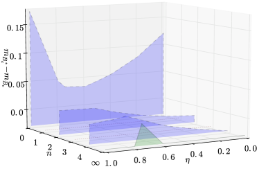
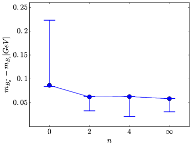
Figure 3: Left panel: $B_{c}^{*}-B_{c}$ mass splitting as a function of $n$ and $\eta$ in our scheme. Right panel: $B_{c}^{*}-B_{c}$ mass splitting as a function of $n$ in our scheme for fixed $\eta=0.75$ (blue circles); error bars indicate variations with respect to $\eta$.

Overall, we find that relative dressing effects are of the order of 30% for the $\rho$ and $K^{*}$, and go down to a few percent for the $B_{c}^{*}$ or even below one percent for the $\Upsilon$. The sizes of relative dressing effects increase with a decrease of either the meson mass or the sum of the quark masses in the meson, which is a natural outcome and interpretation.

Regarding absolute dressing effects we find that these are significantly more pronounced in the vector-meson case than the pseudoscalar one. We also see that a two-loop vertex dressing ($n=2$) already covers half or more of the dressing effect of the full vertex as compared to the RL result, with the remaining difference—except for the light-meson cases—being below 5%.

On another general note, absolute as well as relative dressing effects appear to be of the same order of magnitude for mesons from the categories with equal- or unequal-mass constituents.

In terms of interpretation of RL studies in general we can state that effects are sizeable and worth studying, but at the same time they are systematic and do not a priori destroy the validity and predictive power of a sophisticated and well-controlled RL investigation, which can be useful by utilizing, e. g., mass splittings, trends or cases protected by the symmetries of the theory in a careful and comprehensive manner.

III.2 Mass of the $B_{c}^{*}$

Next, we make a prediction for the mass of the $B_{c}^{*}$ meson. It’s value is as yet unknown experimentally and has been predicted in the literature, e. g., in the quark model (QM) Eichten and Feinberg (1981); Stanley and Robson (1980); Buchmuller and Tye (1981); Godfrey and Isgur (1985); Gershtein et al. (1988); Kaidalov and Nogteva (1988); Kwong and Rosner (1991); Baker et al. (1992); Chen and Kuang (1992); Itoh et al. (1992); Eichten and Quigg (1994); Bagan et al. (1994); Zeng et al. (1995); Roncaglia et al. (1995); Kiselev et al. (1995); Gupta and Johnson (1996); Fulcher (1999); Ebert et al. (2003); Ikhdair and Sever (2003, 2004); Godfrey (2004); Ikhdair and Sever (2005a); Ebert et al. (2011), light-front quark model (LFQM) Frederico et al. (2002); Choi and Ji (2009); Choi et al. (2015), reductions of the BSE (BSR) Abd El-Hady et al. (1999); Baldicchi and Prosperi (2000); Ikhdair and Sever (2005b), with the nonrelativistic renormalization group (NRG) Penin et al. (2004), QCD sum rules (QCDSR) Aliev and Yilmaz (1992); Gershtein et al. (1995); Wang (2013), an RL study in the DSBSE approach (MT-RL) Fischer et al. (2015), and lattice QCD (LAT) Davies et al. (1996); Chiu and Hsieh (2007); Gregory et al. (2010); Dowdall et al. (2012); Burch (2015). In Tab. 2 we compare these results from the literature and add our own, ignoring error bars in each case.

Table 2: Comparison of predictions of the $B_{c}^{*}$ meson mass.

MN Full	MN RL	MT-RLFischer et al. (2015)	LAT Davies et al. (1996)	LAT Chiu and Hsieh (2007)	LAT Gregory et al. (2010)	LAT Dowdall et al. (2012)
6.334	6.362	6.419	6.320	6.315	6.330	6.332
LAT Burch (2015)	NRG Penin et al. (2004)	BSR Abd El-Hady et al. (1999)	BSR Baldicchi and Prosperi (2000)	BSR Ikhdair and Sever (2005b)	QCDSR Aliev and Yilmaz (1992)	QCDSR Gershtein et al. (1995)
6.329	6.323	6.406	6.345	6.316	6.300	6.317
QCDSR Wang (2013)	LFQM Frederico et al. (2002)	LFQM Choi and Ji (2009)	LFQM Choi et al. (2015)	QM Eichten and Feinberg (1981)	QM Stanley and Robson (1980)	QM Buchmuller and Tye (1981)
6.334	6.346	6.310	6.330	6.339	6.346	6.340
QM Godfrey and Isgur (1985)	QM Gershtein et al. (1988)	QM Kaidalov and Nogteva (1988)	QM Kwong and Rosner (1991)	QM Baker et al. (1992)	QM Chen and Kuang (1992)	QM Itoh et al. (1992)
6.340	6.329	6.370	6.321	6.372	6.344	6.328
QM Eichten and Quigg (1994)	QM Bagan et al. (1994)	QM Zeng et al. (1995)	QM Roncaglia et al. (1995)	QM Kiselev et al. (1995)	QM Gupta and Johnson (1996)	QM Fulcher (1999)
6.337	6.330	6.340	6.320	6.317	6.308	6.341
QM Ebert et al. (2003)	QM Ikhdair and Sever (2003)	QM Ikhdair and Sever (2004)	QM Godfrey (2004)	QM Ikhdair and Sever (2005a)	QM Ebert et al. (2011)
6.332	6.324	6.325	6.338	6.329	6.333

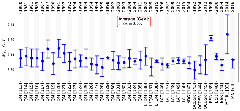
Figure 4: $B_{c}^{*}$ mass values including error bars (blue data points) taken from the references as listed on the lower axis in the figure, corresponding to Tab. 2. Years of appearance are given on the upper axis for each data point. The horizontal red line is the average; its error is about the size of the thickness of the line. Value and error of the average are provided in the insert.

We present two of our own values in this table, namely one for our RL case in column two and the result for the fully dressed setup in column one. The RL result is included to allow better comparison with regard to the RL study and result in Fischer et al. (2015), which uses a more sophisticated effective interaction, the MT-model Maris and Tandy (1999).

Our full result agrees very nicely with the predictions from the various approaches and studies. We obtain the number via calculating the hyperfine mass splitting between the $B_{c}^{*}$ and $B_{c}$ mesons and adding it to the experimentally measured mass of the $B_{c}$, which is $6.275\pm 0.001$ GeV Olive and others (Particle Data Group). We note here that for the DSBSE study of Fischer et al. (2015) we have adjusted their published result in a similar manner, i. e., computed their value of the splitting and added it to the experimental pseudoscalar mass.

Investigating the $\eta$ dependence of this splitting for each $n$ shows again a situation where a very small range of $\eta$ values is available at $n=\infty$ and all values at our chosen $\eta$ are largest or smallest available. This is illustrated in the left and right panels of Fig. 3, where again the dressing effects appear close to minimized by our choice of $\eta$. Plotting our splitting as a function of $n$ in our scheme in the right panel of Fig. 3 we observe that RL truncation overestimates it at $0.087^{+0.136}_{-0.003}$ GeV and corrections reduce its value to the full result of $0.059^{+0.001}_{-0.028}$ GeV. The error bars, also plotted in the figure, again represent the results’ dependence on $\eta$ with the interpretation as a systematic error as explained above. Incorporating the error bar into our result for the $B_{c}^{*}$ mass, we arrive at $6.334^{+0.001}_{-0.028}$ GeV.

To obtain a better picture of the overall comparison of the various results among each other, we have collected them in Fig. 4. The references together with their characteristic as noted in Tab. 2 are given below each data point, while the year of the study is shown above.

For the data points plotted we used the central value of each calculation together with an error bar as follows: For those results, where an error bar is explicitly given in the reference, we include it as provided; where no error bar is provided, we choose a default size for an appropriate error bar via an argument from Ref. Kwong and Rosner (1991), where the authors list an error of $\pm 0.036$ GeV for their quark-model result in order to “get an idea of systematic errors inherent in quark models”. Concretely, we set the default error to $\pm 0.03$ GeV, which provides a reasonable picture as well as a solid basis for the next step: to arrive at an interesting estimate of the overall theory prediction for the mass of the $B_{c}^{*}$, we perform a standard weighted average of all values and errors, whose result is inserted in Fig. 4 and also plotted underneath the data as a horizontal red line. For the two cases of asymmetric errors we treated the average of the upper and lower error as a symmetric error instead to simplify the procedure. The averaged result is $6.336\pm 0.002$ GeV, which may serve as a more suitable number to compare to than the individual theoretical results.

III.3 Quark-Photon Vertex

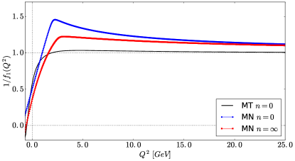
Figure 5: Inverse of transversal component $1/f_{1}$ of the quark-photon vertex for different $n$ in the MN model studied herein together with a sophisticated (Maris-Tandy, MT) model Maris and Tandy (1999) result in RL truncation for comparison, see text. Left panel: Detailed view in region around $Q^{2}=0$; Right panel: large-scale view without error bars on the MN curves to emphasize the asymptotic behavior.

A case of immediate interest in the investigation of the quantum numbers $J^{PC}=1^{--}$ is the dressed quark-photon vertex Maris and Tandy (2000, 2002, 2006); Eichmann (2014). It can be obtained consistently from the inhomogeneous version of the vector BSE, which is a straight-forward computation once the BSE kernel has been defined and computed Bhagwat et al. (2007a); Blank and Krassnigg (2011b, c).

The vertex has the general structure

$$\Gamma_{\mu}(Q;k)=\Gamma_{\mu}^{L}(Q;k)+\sum_{i=1}^{8}T^{i}_{\mu}(Q;k)f_{i}(Q;k)\;,$$ (15)

where the arguments are the relative quark-antiquark momentum $k$ and the (photon) total momentum $Q$, the eight covariants $T_{\mu}^{i}$ are transverse with respect to $Q$, and the longitudinal part $\Gamma_{\mu}^{L}(Q;k)$ is fixed via the vector Ward-Takahashi identity and can be written in the Ball-Chiu construction Ball and Chiu (1980) as the longitudinal projection with respect to $Q$ of

$$\Gamma_{\mu}^{\mathrm{BC}}(Q;k) = i\;\gamma_{\mu}\Sigma_{A}(Q;k)$$ (16)

$$+ 2k_{\mu}[i\;k\cdot\gamma\;\Delta_{A}(Q;k)+\Delta_{B}(Q;k)]\;.$$

In particular,

$$\Sigma_{A}(Q;k) = \frac{A(k_{+}^{2})+A(k_{-}^{2})}{2}\;,$$ (17)

$$\Delta_{A}(Q;k) = \frac{A(k_{+}^{2})-A(k_{-}^{2})}{k_{+}^{2}-k_{-}^{2}}\;,$$ (18)

$$\Delta_{B}(Q;k) = \frac{B(k_{+}^{2})-B(k_{-}^{2})}{k_{+}^{2}-k_{-}^{2}}\;,$$ (19)

with the (anti)quark momenta $k_{\pm}$ defined analogously as in the homogeneous BSE above as $k_{+}=k+\eta Q$ and $k_{-}=k-(1-\eta)Q$, which entails

$$k_{+}^{2} = k^{2}+2\eta\;k\cdot Q+\eta^{2}Q^{2}\;,$$ (20)

$$k_{-}^{2} = k^{2}-2(1-\eta)\;k\cdot Q+(1-\eta)^{2}Q^{2}\;,$$ (21)

$$k_{+}^{2}-k_{-}^{2} = (2\eta-1)(2\;k\cdot Q+Q^{2})\;.$$ (22)

In our case, after the simplification via Eq. (1), we remain with

$$k_{+}^{2} = \eta^{2}Q^{2}\;,$$ (23)

$$k_{-}^{2} = (1-\eta)^{2}Q^{2}\;,$$ (24)

$$k_{+}^{2}-k_{-}^{2} = (2\eta-1)Q^{2}\;.$$ (25)

and thus

$$\Sigma_{A}(Q) = \frac{A(\eta^{2}Q^{2})+A((1-\eta)^{2}Q^{2})}{2}\;,$$ (26)

$$\Delta_{A}(Q) = \frac{A(\eta^{2}Q^{2})-A((1-\eta)^{2}Q^{2})}{(2\eta-1)Q^{2}}\;,$$ (27)

$$\Delta_{B}(Q) = \frac{B(\eta^{2}Q^{2})-B((1-\eta)^{2}Q^{2})}{(2\eta-1)Q^{2}}\;.$$ (28)

In the case of the quark-photon vertex, the quark and antiquark in the BSE have equal flavor and mass due to the nature of the electromagnetic interaction. For the standard setting in such a case, $\eta=0.5$, we obtain

$$k_{+}^{2}=k_{-}^{2} = Q^{2}/4\;,$$ (29)

$$\Sigma_{A}(Q) = A(Q^{2}/4)\;,$$ (30)

$$\Delta_{A}(Q) = A^{\prime}(Q^{2}/4)\;,$$ (31)

$$\Delta_{B}(Q) = B^{\prime}(Q^{2}/4)\;,$$ (32)

so that under normal circumstances with finite values of $A^{\prime}(Q^{2}/4)$ and $B^{\prime}(Q^{2}/4)$, the Ball-Chiu vertex reduces to

$$\Gamma_{\mu}^{\mathrm{BC}}(Q) = i\;\gamma_{\mu}\;A(Q^{2}/4)\;.$$ (33)

As we discuss herein, explicitly in App. B, for the transverse vector covariants, only 2 are left nonzero by the model’s simplifications and one can easily solve the inhomogeneous BSE to obtain the corresponding solutions.

In Fig. 5 we plot the nonzero amplitudes as functions of the total momentum squared to illustrate the size of dressing effects for the dressed quark-photon vertex in our (MN) scheme. The quark mass is chosen to be the light-quark mass. The most prominent sets to look at are the case $n=0$, which corresponds to the rainbow-ladder-truncation result and is depicted by the blue disks, and $n=\infty$, which represents the result from the fully dressed QGV and is depicted by the red boxes. In addition, to highlight the rapid convergence of this function in our scheme, we also plotted the cases $n=2$ and $n=4$, which are almost on top of the $n=\infty$ result; however, in order not to overcrowd the figure, odd values of $n$ are left out here.

In short, the difference between the RL truncated result and any of the dressed versions is sizeable, while all dressed solutions among themselves are hard to distinguish, and differences are minor. In absence of the dependence on a relative momentum squared, the behavior seen here may well be interpreted as the prototype of variation of the $P^{2}$-dependence of elements of the quark-photon vertex beyond RL truncation in the sense that already the first order in our scheme provides a result close to the fully dressed case.

In each case, we have, as required by our own statements, studied the model-artificial $\eta$ dependence of the MN results and depicted the variation via error bars on each of the curves. As it turns out, such a dependence is stronger for larger values of $Q^{2}$ and negligible around $Q^{2}=0$. The central curve is always given by the natural choice of $\eta=0.5$.

To complete the picture, we also plot the corresponding component for a dressed quark-photon vertex obtained with a sophisticated model interaction (the Maris-Tandy/MT model Maris and Tandy (1999)) in RL truncation in analogy to the study in Maris and Tandy (2000). More precisely, we plot the inverse of the zeroth Chebyshev moment at zero relative momentum squared as a function of $Q^{2}$, which corresponds to our MN-RL curve and serves as a baseline to impose putative dressing effects as they are studied here. This kind of comparison is supported as a result of the calculational restrictions due to the truncation scheme’s adherence to the symmetry requirements of the theory represented by the relevant WTIs, which are respected in both the MT and MN cases, as discussed above.

In the figure we have also plotted three dotted lines for ease of orientation, namely: a horizontal line at $1/f_{1}=0$, which clearly shows the position of zeros in each curve, i. e., the $\rho$-pole positions—note that such a pole contribution is present in every single case; a vertical line at $Q^{2}=0$, which marks the transition from the timelike to the spacelike region of photon momentum; finally, a horizontal line at $1/f_{1}=1$, which indicates the limit of the asymptotic behavior of all curves for $Q^{2}\rightarrow\infty$, i. e., the perturbative limit in which all curves agree by construction.

To better illustrate both the details of the various curves as well as their asymptotic behavior, we provide two panels in Fig. 5: the left panel shows a detailed view of the region around $Q^{2}=0$, includes error bars as well as multiple curves from the MN truncation scheme. The right panel on the other hand shows only three curves without error bars and very nicely documents them approaching the perturbative limit.

IV Conclusions

We have extended earlier DSBSE studies in a systematic truncation scheme using a simple effective-interaction model together with a dressed QGV to the unequal-mass case of vector mesons. After a general analysis of dressing effects in both the quarkonia and the various flavored mesons, we focused on two items of special interest, namely the mass of the $B_{c}^{*}$ meson and the dressed quark-photon vertex.

The general pattern of dressing effects confirms expectations where dressing effects beyond RL truncation are the stronger, the lighter the involved quark content is. We found, rather importantly, that such effects are more pronounced in the vector-meson case than in the pseudoscalar case studied earlier. This entails that mass (such as hyperfine) splittings are modified significantly by corrections in a systematic truncation scheme such as the one presented here.

Using such a calculated splitting between the $B_{c}^{*}$ and the $B_{c}$ mesons, we predict the mass of the former and put our result in the context of other predictions available in the literature. Our number, $6.334^{+0.001}_{-0.028}$ GeV compares well with the rest of the literature, and our comparison to the RL result sheds some light on possible changes of corresponding results at higher order in a systematic scheme such as the one presented here.

In addition we have provide an average of a comprehensive set of results from the theory literature. The averaged result for the mass of the $B_{c}^{*}$ meson is $6.336\pm 0.002$ GeV.

To obtain results for the dressed quark-photon vertex, we present solutions for the inhomogeneous vector-vertex BSE for the first time in the context of a truncation scheme. Our simple-model convergence picture is contrasted to an RL calculation with a more sophisticated model interaction and analogies are discussed in detail.

Our results support both studies of corrections to RL truncation as well as sophisticated and well-controlled RL studies as such, since they can be performed with a much more comprehensive scope in mind. Furthermore, we have once again demonstrated the strength of the use of mass splittings as tools with predictive power in our approach.

Appendix A $\eta$-dependence of meson masses

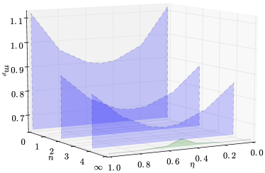
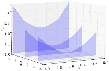
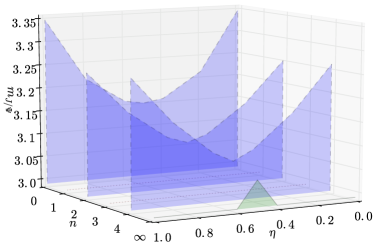
Figure 6: Meson bound-state masses as functions of $n$ and $\eta$, given in GeV. Even $n$ are depicted by dashed lines, odd ones by dotted lines, and the fully summed result by a solid line. If no solution is found, no surface is plotted at the corresponding $n$. Left upper panel: $\rho$; right upper panel: $\varphi$; eft lower panel: $J/\Psi$; right lower panel: $\Upsilon$.

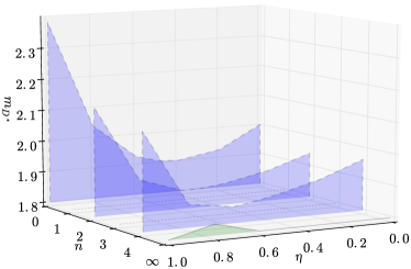
Figure 7: Same as Fig. 6: Left upper panel: $K^{*}$; right upper panel: $D^{*}$; left center panel: $B^{*}$; right center panel: $D_{s}^{*}$; left lower panel: $B_{s}^{*}$; right lower panel: $B_{c}^{*}$.

In this appendix we collect data and plots about the details of the dependence of the meson masses on the momentum-partitioning parameter $\eta$ as a function of the order $n$ in our scheme. The corresponding plots are shown in the various panels of Figs. 6 and 7 for the equal- and unequal-mass cases, respectively. The alternating pattern of convergence of the odd and even $n$ numbers described earlier in Gomez-Rocha et al. (2015b) is difficult to observe herein, since there is, again, a distinct lack of solutions for odd $n$ on our main $\eta$ grid points. Still, convergence with $n$ is observed as well as a pronounced $\eta$ asymmetry for the heavy-light case, which is the source of the large error bars plotted in Fig. 1. Despite this artificial behavior a detailed study such as ours remains true to the systematic character of both the approach and the truncation scheme presented here and, in particular, validates the qualitative as well as quantitative statements made above.

Appendix B vector kernel details

Following Refs. Bender et al. (2002); Bhagwat et al. (2004); Gomez-Rocha et al. (2015b) we collect the details of the BSA, the correction term $\Lambda$, and the QGV in this appendix. The recursion relations for the QGV $\Gamma_{\mu}$, Eq. (6) and the BSE correction term $\Lambda_{M\mu}$, Eq. (11) are detailed, in particular with respect to Dirac structures.

From the 12 covariant structures of the full QGV, Eq. (1) reduces this set to three nonzero ones:

$$\Gamma_{\mu}(p)=\alpha_{1}(p^{2})\gamma_{\mu}+\alpha_{2}(p^{2})\gamma\cdot p\;p_{\mu}-i\alpha_{3}(p^{2})p_{\mu}\;.$$ (34)

With the initial condition that the QGV be bare

$$\Gamma_{\mu}(p)^{0}=\gamma_{\mu}$$ (35)

one can construct the QGV via its recursion relation at any order by expressing the functions $(\alpha_{1},\alpha_{2},\alpha_{3})$ given in Eq. (34) in terms of the quark propagator dressing functions $A$ and $B$. By inserting the result back into the quark DSE one obtains algebraic equations for $A(s)$ and $B(s)$ via Dirac-trace projections onto the two covariant quark propagator structures.

In order to compute $\Lambda_{M\mu}(P)$ a suitable decomposition in terms of Dirac covariants has to be found, depending on the quantum numbers appropriate for the meson $M$ under consideration, in our case vector. In our setup the vector BSA has 2 non-vanishing components from the eight general structures, namely:

$$\Gamma_{1^{-}}^{\xi}(P)=f_{1}(P^{2})\;\gamma\cdot\varepsilon^{\xi}(P)-f_{2}(P^{2})\,\sigma_{\mu\nu}\;\varepsilon^{\xi}_{\mu}(P)\hat{P}_{\nu}$$ (36)

with the unit vector $\hat{P}:=P/\sqrt{P^{2}}$ and

$$\sigma_{\mu\nu}\;a_{\mu}b_{\nu}:=\frac{i}{2}(\gamma\cdot a\;\gamma\cdot b-\gamma\cdot b\;\gamma\cdot a)\;.$$ (37)

$\varepsilon^{\xi}_{\mu}(P)$, $\xi=1,2,3$ are polarization vectors with respect to $P$. The corresponding Dirac projections are

$$\mathcal{F}_{1}^{\xi} := \frac{1}{12}\gamma\cdot\varepsilon^{\xi}(P)\;,$$ (38)

$$\mathcal{F}_{2}^{\xi} := -\frac{1}{12}\sigma_{\mu\nu}\;\varepsilon^{\xi}_{\mu}(P)\hat{P}_{\nu}\;,$$ (39)

such that

$$\mathrm{Tr}\sum_{\xi}\left[\mathcal{F}_{j}^{\xi}\Gamma_{1^{-}}^{\xi}(P)=f_{j}(P^{2})\right],\quad j=1,2\;.$$ (40)

We construct $\Lambda_{1^{-}\mu}$ following Bender et al. (2002) for direct comparability as

$$\Lambda_{\mu}^{\xi}(P) = \beta_{1}(P^{2})\,\varepsilon^{\xi}_{\mu}(P)$$ (41)

$$+ \beta_{2}(P^{2})\,i\varepsilon^{\xi}_{\mu}(P)\;\gamma\cdot\hat{P}$$

$$+ \beta_{3}(P^{2})\,i\hat{P}_{\mu}\;\gamma\cdot\varepsilon^{\xi}(P)$$

$$- \beta_{4}(P^{2})\,\sigma_{\tau\nu}\;\varepsilon^{\xi}_{\tau}(P)\hat{P}_{\nu}\;\gamma_{\mu}\;$$

$$- \beta_{5}(P^{2})\,i\sigma_{\tau\nu}\;\varepsilon^{\xi}_{\tau}(P)\hat{P}_{\nu}\;\hat{P}_{\mu}\;$$

$$+ \beta_{6}(P^{2})\,\gamma\cdot\varepsilon^{\xi}(P)\;\gamma_{\mu}\;,$$

where the subscript denoting the vector case has been omitted. The corresponding Dirac projections are

$$\mathcal{P}^{\xi}_{\mu,1} := \frac{1}{4}\varepsilon^{\xi}_{\mu}(P)\;,$$ (42)

$$\mathcal{P}^{\xi}_{\mu,2} := -\frac{i}{4}\varepsilon^{\xi}_{\mu}(P)\;\gamma\cdot\hat{P}\;,$$ (43)

$$\mathcal{P}^{\xi}_{\mu,3} := -\frac{i}{4}\hat{P}_{\mu}\;\gamma\cdot\varepsilon^{\xi}(P)\;,$$ (44)

$$\mathcal{P}^{\xi}_{\mu,4} := -\frac{1}{4}\sigma_{\tau\nu}\;\varepsilon^{\xi}_{\tau}(P)\hat{P}_{\nu}\;\gamma_{\mu}\;,$$ (45)

$$\mathcal{P}^{\xi}_{\mu,5} := \frac{i}{4}\sigma_{\tau\nu}\;\varepsilon^{\xi}_{\tau}(P)\hat{P}_{\nu}\;\hat{P}_{\mu}\;,$$ (46)

$$\mathcal{P}^{\xi}_{\mu,6} := \frac{1}{4}\gamma\cdot\varepsilon^{\xi}(P)\;\gamma_{\mu}\;,$$ (47)

such that

$$\beta_{j}=(\mathcal{M})_{jk}\mathrm{Tr}\sum_{\xi}\left[\mathcal{P}^{\xi}_{\mu,k}\Lambda^{\xi}_{\mu}\right]\;,$$ (48)

where the matrix $\mathcal{M}$ (the vector case $1^{-}$ is assumed implicitly from now on) is given by

$$\mathcal{M}=\frac{1}{2}\left(\begin{array}[]{cccccc}3&0&0&0&1&-1\\ 0&3&-1&-1&0&0\\ 0&-1&3&1&0&0\\ 0&-1&1&1&0&0\\ 1&0&0&0&3&-1\\ -1&0&0&0&-1&1\\ \end{array}\right)\;.$$ (49)

The scalar functions $\vec{\beta}:=\{\beta_{j}\}$, $j=1,\ldots,6$ are obtained at a particular order $n$ in the truncation via the recursion relation (11), resulting in

$$\vec{\beta}^{i}=\mathcal{M}\left(\mathbf{G}_{-}\,\vec{\alpha}_{-}^{\,i-1}+\mathbf{G}_{+}\,\vec{\alpha}_{+}^{\,i-1}+\mathbf{L}\,\vec{\beta}^{\,i-1}\right),$$ (50)

which can be evaluated when the matrices $\mathbf{G}_{\pm}$ and $\mathbf{L}$ are known. $\vec{\alpha}_{+}$ and $\vec{\alpha}_{-}$ denote the coefficients of the QGV decomposition corresponding to the ₊ and _- arguments appearing in their defining quark propagators as given above. With the definitions

$$B_{-} := B(p_{-}^{2})\;,$$ (51)

$$B_{+} := B(p_{+}^{2})\;,$$ (52)

$$A_{-} := (\eta-1)\,\sqrt{P^{2}}A(p_{-}^{2})\;,$$ (53)

$$A_{+} := \eta\,\sqrt{P^{2}}A(p_{+}^{2})\;,$$ (54)

and

$$\Delta_{-} := A_{-}^{2}+B_{-}^{2}\;,$$ (55)

$$\Delta_{+} := A_{+}^{2}+B_{+}^{2}\;,$$ (56)

as well as

$$\Theta_{-} := A_{-}A_{+}-B_{-}B_{+}\;,$$ (57)

$$\Theta_{+} := A_{-}A_{+}+B_{-}B_{+}\;,$$ (58)

$$\Xi_{-} := A_{-}B_{+}-A_{+}B_{-}\;,$$ (59)

$$\Xi_{+} := A_{-}B_{+}+A_{+}B_{-}\;,$$ (60)

and

$$\Phi_{-} := B_{+}A_{-}^{2}-2A_{-}A_{+}B_{-}-B_{+}B_{-}^{2}\;,$$ (61)

$$\Phi_{+} := A_{+}A_{-}^{2}+2A_{-}B_{-}B_{+}-A_{+}B_{-}^{2}\;,$$ (62)

$$\Psi_{-} := B_{-}A_{+}^{2}-2A_{-}A_{+}B_{+}-B_{-}B_{+}^{2}\;,$$ (63)

$$\Psi_{+} := A_{-}A_{+}^{2}+2A_{+}B_{-}B_{+}-A_{-}B_{+}^{2}\;,$$ (64)

one obtains

$$\mathcal{M}\mathbf{L}=\frac{2\mathcal{C}}{\Delta_{-}\,\Delta_{+}}\left(\begin{array}[]{cccccc}2\Theta_{-}&-2\Xi_{+}&0&-2\Xi_{+}&0&2\Theta_{-}\\ -\Xi_{+}&-\Theta_{-}&0&-2\Theta_{-}&0&-2\Xi_{+}\\ 0&0&\Theta_{+}&-2B_{-}B_{+}&-\Xi_{-}&2B_{-}A_{+}\\ 0&0&0&\Theta_{-}&0&\Xi_{+}\\ 0&0&0&0&0&0\\ 0&0&0&0&0&0\\ \end{array}\right)\;.$$ (65)

In the equal-mass case, as presented in Bender et al. (2002) one obtains

$$\mathcal{M}\mathbf{L}=\frac{1}{4\Delta^{2}}\left(\begin{array}[]{cccccc}2\Delta&0&0&0&0&2\Delta\\ 0&-\Delta&0&-2\Delta&0&0\\ 0&0&A^{2}Q^{2}-B^{2}&2B^{2}&-2AB\sqrt{Q^{2}}&-2AB\sqrt{Q^{2}}\\ 0&0&0&\Delta&0&0\\ 0&0&0&0&0&0\\ 0&0&0&0&0&0\\ \end{array}\right)$$ (66)

with the replacements $\mathcal{C}\rightarrow-\frac{1}{8}$ and $P^{2}\rightarrow 4Q^{2}$, which is identical to the result given in Bender et al. (2002) except for a factor of $2$ in element $(3,3)$ of this matrix.

The two matrices $\mathbf{G}_{-}$ and $\mathbf{G}_{+}$ are associated with the corresponding quark propagators with the ₊ and _- arguments as defined above:

$$\mathcal{M}\mathbf{G}_{-}=\frac{-\mathcal{C}}{\Delta_{-}^{2}\Delta_{+}}\left(\begin{array}[]{ccc}-4\Delta_{-}B_{+}f_{1}-4\Delta_{-}A_{+}f_{2}&0&0\\ -4\Delta_{-}A_{+}f_{1}+4\Delta_{-}B_{+}f_{2}&0&0\\ -4B_{-}\Xi_{-}f_{1}-4B_{-}\Theta_{+}f_{2}&-2q_{-}^{2}\Phi_{+}f_{1}+2q_{-}^{2}\Phi_{-}f_{2}&-2\sqrt{q_{-}^{2}}\Phi_{-}f_{1}-2\sqrt{q_{-}^{2}}\Phi_{+}f_{2}\\ 2\Delta_{-}A_{+}f_{1}-2\Delta_{-}B_{+}f_{2}&0&0\\ 0&0&0\\ 0&0&0\\ \end{array}\right)\;,$$ (67)

which is to be understood as a $6\times 3$ matrix, and its corresponding analog

$$\mathcal{M}\mathbf{G}_{+}=\frac{-\mathcal{C}}{\Delta_{-}\Delta_{+}^{2}}\left(\begin{array}[]{ccc}-4B_{-}\Delta_{+}f_{1}+4A_{-}\Delta_{+}f_{2}&0&0\\ 0&0&0\\ -4A_{+}\Theta_{+}f_{1}+4\Xi_{-}A_{+}f_{2}&-2q_{+}^{2}\Psi_{+}f_{1}-2q_{+}^{2}\Psi_{-}f_{2}&2\sqrt{q_{+}^{2}}\Psi_{-}f_{1}-2\sqrt{q_{+}^{2}}\Psi_{+}f_{2}\\ -2A_{-}\Delta_{+}f_{1}-2B_{-}\Delta_{+}f_{2}&0&0\\ 0&0&0\\ 0&0&0\\ \end{array}\right)\;.$$ (68)

In the equal-mass case, again with the replacements $\mathcal{C}\rightarrow-\frac{1}{8}$ and $P^{2}\rightarrow 4Q^{2}$ this becomes

$$\mathcal{M}(\mathbf{G}_{-}+\mathbf{G}_{+})=\frac{1}{2\Delta^{2}}\left(\begin{array}[]{ccc}2\left(Bf_{1}+A\sqrt{Q^{2}}f_{2}\right)&0&0\\ A\sqrt{Q^{2}}f_{1}-Bf_{2}&0&0\\ -A\sqrt{Q^{2}}f_{1}+Bf_{2}&0&0\\ -A\sqrt{Q^{2}}f_{1}+Bf_{2}&0&0\\ 0&0&0\\ 0&0&0\\ \end{array}\right)\;,$$ (69)

which is identical to the result given in Bender et al. (2002) except for an overall factor of $1/\Delta$.

Appendix C Proof of Kernel Construction

In this appendix we present a short proof that our kernel construction in fact satisfies the Axial-Vector Ward-Takahashi Identity (AVWTI), as required by the general setup of the truncation scheme. The AVWTI can be written in its integral form as Eichmann (2009)

$$\int_{q}^{\Lambda}\left\{S(q_{+})\gamma_{5}+\gamma_{5}S(q_{-})\right\}_{GH}K^{GH}_{EF}(k,q,P)$$

$$=\{\Sigma(k_{+})\gamma_{5}+\gamma_{5}\Sigma(k_{-})\}_{EF}\;,$$ (70)

where $K$ is the quark-antiquark scattering kernel used in the meson BSE, $q_{\pm}$ are the (anti)quark momenta, and $EFGH$ denote color, Dirac, and flavor indices.

In the following, we show that the kernel in Eq. (9) satisfies this equation. Alternatively, one can in principle also reverse the argument to arrive at the kernel construction starting out from the AVWTI.

The gluon-loop dressed QGV correction term to the BSE kernel, as defined in Eqs. (10) and (11), leads to a corresponding correction to the AVWTI of the form

$$\bar{\Lambda}^{M}_{\nu}(P)=\sum_{i=0}^{\infty}\bar{\Lambda}_{\nu,i}^{M}(P)\,,$$ (71)

with

$$\frac{1}{\mathcal{C}}\bar{\Lambda}_{\nu,n}^{M}(P)=$$

$$-\gamma_{\rho}\left\{S(q_{+})\gamma_{5}+\gamma_{5}S(q_{-})\right\}\Gamma_{\nu,n-1}^{\mathcal{C}}(q_{-})S(q_{-})\gamma_{\rho}$$

$$-\gamma_{\rho}S(q_{+})\Gamma_{\nu,n-1}^{\mathcal{C}}(q_{+})\left\{S(q_{+})\gamma_{5}+\gamma_{5}S(q_{-})\right\}\gamma_{\rho}$$

$$-\gamma_{\rho}S(q_{+})\bar{\Lambda}_{\nu,n-1}^{M}(P)S(q_{-})\gamma_{\rho}\;.$$ (72)

Using the recursion relation for the QGV (6), this becomes

$$\frac{1}{\mathcal{C}}\bar{\Lambda}_{\nu,n}^{M}(P)=$$

$$-\gamma_{\rho}S(q_{+})\gamma_{5}\Gamma_{\nu,n-1}^{\mathcal{C}}(q_{-})S(q_{-})\gamma_{\rho}-\gamma_{5}\Gamma_{\nu,n}^{\mathcal{C}}(q_{-})$$

$$-\Gamma_{\nu,n}^{\mathcal{C}}(q_{+})\gamma_{5}-\gamma_{\rho}S(q_{+})\Gamma_{\nu,n-1}^{\mathcal{C}}(q_{+})\gamma_{5}S(q_{-})\gamma_{\rho}$$

$$-\gamma_{\rho}S(q_{+})\bar{\Lambda}_{\nu,n-1}^{M}(P)S(q_{-})\gamma_{\rho}\;.$$ (73)

Upon insertion of the lower-order correction term $\bar{\Lambda}_{\nu,n-1}^{M}(P)$ in Eq. (73), it can be seen that the first and fourth term in Eq. (73) are canceled by the second and third term of the $\bar{\Lambda}_{\nu,n-1}^{M}(P)$ contribution.

Therefore, the recursion (73) collapses to

$$\frac{1}{\mathcal{C}}\bar{\Lambda}_{\nu,n}^{M}(P)= -\gamma_{\rho}S(q_{+})\gamma_{5}\Gamma_{\nu,0}^{\mathcal{C}}(q_{-})S(q_{-})\gamma_{\rho}-\gamma_{5}\Gamma_{\nu,n}^{\mathcal{C}}(q_{-})$$ (74)

$$-\Gamma_{\nu,n}^{\mathcal{C}}(q_{+})\gamma_{5}-\gamma_{\rho}S(q_{+})\Gamma_{\nu,0}^{\mathcal{C}}(q_{+})\gamma_{5}S(q_{-})\gamma_{\rho}$$

$$-\gamma_{\rho}S(q_{+})\bar{\Lambda}_{\nu,0}^{M}(P)S(q_{-})\gamma_{\rho}\;.$$

From $\Lambda_{\nu,0}^{M}(P)=0$, it follows that $\bar{\Lambda}_{\nu,0}^{M}(P)=0$.

Because of $\Gamma_{\nu,0}^{\mathcal{C}}(q_{\pm})=\gamma_{\nu}$ and the anticommutation properties of the Clifford-algebra, the first and fourth term cancel each other and Eq. (74) reduces to

$$\frac{1}{\mathcal{C}}\bar{\Lambda}_{\nu,n}^{M}(P)=-\gamma_{5}\Gamma_{\nu,n}^{\mathcal{C}}(q_{-})-\Gamma_{\nu,n}^{\mathcal{C}}(q_{+})\gamma_{5}\;.$$ (75)

Hence,

$$\frac{1}{\mathcal{C}}\bar{\Lambda}_{\nu}^{M}(P)=-\gamma_{5}\Gamma_{\nu}^{\mathcal{C}}(q_{-})-\Gamma_{\nu}^{\mathcal{C}}(q_{+})\gamma_{5}\;.$$ (76)

The AVWTI becomes

$$\int_{q}^{\Lambda}\left\{S(q_{+})\gamma_{5}+\gamma_{5}S(q_{-})\right\}_{GH}K^{GH}_{EF}(k,q,P)$$

$$=-\frac{1}{2}\Bigl{[}\gamma_{\nu}\left\{S(k_{+})\gamma_{5}+\gamma_{5}S(k_{-})\right\}\Gamma_{\nu}^{\mathcal{C}}(k_{-})\Bigr{.}$$

$$+\Gamma_{\nu}^{\mathcal{C}}(k_{+})\left\{S(k_{+})\gamma_{5}+\gamma_{5}S(k_{-})\right\}\gamma_{\nu}$$

. $$+\gamma_{\nu}S(k_{+})\bar{\Lambda}_{\nu}^{M}(P)+\bar{\Lambda}_{\nu}^{M}(P)S(k_{-})\gamma_{\nu}\Bigr{]}_{EF}$$ (79)

$$=\{\gamma_{\nu}S(k_{+})\Gamma_{\nu}^{\mathcal{C}}(k_{+})\gamma_{5}+\gamma_{5}\gamma_{\nu}S(k_{-})\Gamma_{\nu}^{\mathcal{C}}(k_{-})\}_{EF}$$

$$=\{\Sigma(k_{+})\gamma_{5}+\gamma_{5}\Sigma(k_{-})\}_{EF}\;,$$

which is the desired result, where

$$\gamma_{\mu}S(p)\Gamma_{\mu}(p)=\Gamma_{\mu}(p)S(p)\gamma_{\mu}$$ (80)

has been used.

Appendix D Algebraic gap equations

In our recursive setup, the coupled equations for the various dressing functions contain polynomials of increasing order with increasing order in the recursion. The fully summed solution is obtained via a geometric sum and thus produces equations involving polynomials of a finite order as well.

Here we present the algebraic equations resulting for $A$ and $B$ at the orders used in our study, namely $n=0,1,2,3,4,\infty$, including explicitly the current-quark mass $m$, the coupling $\mathcal{G}$ as well as the strength parameter $\mathcal{C}$.

For $n=0$ one has RL truncation and the Dirac-projected gap equations for $A$ and $B$ read

$$A = 1+\frac{2A\mathcal{G}}{\Delta}\;,$$ (81)

$$B = m+\frac{4B\mathcal{G}}{\Delta}\;.$$ (82)

For $n=1$ the Dirac-projected gap equations for $A$ and $B$ read

$$A = 1+\frac{2A\mathcal{G}}{\Delta}+\frac{8A\mathcal{C}\mathcal{G}^{2}}{\Delta^{2}}+\frac{4AB^{2}\mathcal{C}\mathcal{G}^{2}}{\Delta^{3}}\;,$$ (83)

$$B = m+\frac{4B\mathcal{G}}{\Delta}+\frac{12B\mathcal{C}\mathcal{G}^{2}}{\Delta^{2}}-\frac{4B^{3}\mathcal{C}\mathcal{G}^{2}}{\Delta^{3}}\;.$$ (84)

For $n=2$ the Dirac-projected gap equations for $A$ and $B$ read

$$A = 1+\frac{2A\mathcal{G}}{\Delta}+\frac{8A\mathcal{C}\mathcal{G}^{2}}{\Delta^{2}}+\frac{4A\mathcal{C}\mathcal{G}^{2}\left(B^{2}+2\mathcal{C}\mathcal{G}\right)}{\Delta^{3}}-\frac{16AB^{4}\mathcal{C}^{2}\mathcal{G}^{3}}{\Delta^{5}}\;,$$ (85)

$$B = m+\frac{4B\mathcal{G}}{\Delta}+\frac{12B\mathcal{C}\mathcal{G}^{2}}{\Delta^{2}}-\frac{4B\mathcal{C}\mathcal{G}^{2}\left(B^{2}-8\mathcal{C}\mathcal{G}\right)}{\Delta^{3}}-\frac{32B^{3}\mathcal{C}^{2}\mathcal{G}^{3}}{\Delta^{4}}+\frac{16B^{5}\mathcal{C}^{2}\mathcal{G}^{3}}{\Delta^{5}}\;.$$ (86)

For $n=3$ the Dirac-projected gap equations for $A$ and $B$ read

$$A = 1+\frac{2A\mathcal{G}}{\Delta}+\frac{8A\mathcal{C}\mathcal{G}^{2}}{\Delta^{2}}+\frac{4A\mathcal{C}\mathcal{G}^{2}\left(B^{2}+2\mathcal{C}\mathcal{G}\right)}{\Delta^{3}}+\frac{32A\mathcal{C}^{3}\mathcal{G}^{4}}{\Delta^{4}}-\frac{16AB^{2}\mathcal{C}^{2}\mathcal{G}^{3}\left(B^{2}-3\mathcal{C}\mathcal{G}\right)}{\Delta^{5}}$$ (87)

$$-\frac{32AB^{4}\mathcal{C}^{3}\mathcal{G}^{4}}{\Delta^{6}}+\frac{64AB^{6}\mathcal{C}^{3}\mathcal{G}^{4}}{\Delta^{7}}\;,$$

$$B = m+\frac{4B\mathcal{G}}{\Delta}+\frac{12B\mathcal{C}\mathcal{G}^{2}}{\Delta^{2}}-\frac{4\left(B^{3}\mathcal{C}\mathcal{G}^{2}-8B\mathcal{C}^{2}\mathcal{G}^{3}\right)}{\Delta^{3}}-\frac{16\left(2B^{3}\mathcal{C}^{2}\mathcal{G}^{3}-7B\mathcal{C}^{3}\mathcal{G}^{4}\right)}{\Delta^{4}}$$ (88)

$$+\frac{16\left(B^{5}\mathcal{C}^{2}\mathcal{G}^{3}-11B^{3}\mathcal{C}^{3}\mathcal{G}^{4}\right)}{\Delta^{5}}+\frac{160B^{5}\mathcal{C}^{3}\mathcal{G}^{4}}{\Delta^{6}}-\frac{64B^{7}\mathcal{C}^{3}\mathcal{G}^{4}}{\Delta^{7}}\;.$$

For $n=4$ the Dirac-projected gap equations for $A$ and $B$ read

$$A = 1+\frac{2A\mathcal{G}}{\Delta}+\frac{8A\mathcal{C}\mathcal{G}^{2}}{\Delta^{2}}+\frac{4\left(AB^{2}\mathcal{C}\mathcal{G}^{2}+2A\mathcal{C}^{2}\mathcal{G}^{3}\right)}{\Delta^{3}}+\frac{32A\mathcal{C}^{3}\mathcal{G}^{4}}{\Delta^{4}}+\frac{16\left(-AB^{4}\mathcal{C}^{2}\mathcal{G}^{3}+3AB^{2}\mathcal{C}^{3}\mathcal{G}^{4}+2A\mathcal{C}^{4}\mathcal{G}^{5}\right)}{\Delta^{5}}$$ (89)

$$+\frac{32\left(2AB^{2}\mathcal{C}^{4}\mathcal{G}^{5}-AB^{4}\mathcal{C}^{3}\mathcal{G}^{4}\right)}{\Delta^{6}}-\frac{64\left(6AB^{4}\mathcal{C}^{4}\mathcal{G}^{5}-AB^{6}\mathcal{C}^{3}\mathcal{G}^{4}\right)}{\Delta^{7}}-\frac{256AB^{8}\mathcal{C}^{4}\mathcal{G}^{5}}{\Delta^{9}}+\frac{256AB^{6}\mathcal{C}^{4}\mathcal{G}^{5}}{\Delta^{8}}\;,$$

$$B = m+\frac{4B\mathcal{G}}{\Delta}+\frac{12B\mathcal{C}\mathcal{G}^{2}}{\Delta^{2}}-\frac{4\left(B^{3}\mathcal{C}\mathcal{G}^{2}-8B\mathcal{C}^{2}\mathcal{G}^{3}\right)}{\Delta^{3}}-\frac{16\left(2B^{3}\mathcal{C}^{2}\mathcal{G}^{3}-7B\mathcal{C}^{3}\mathcal{G}^{4}\right)}{\Delta^{4}}$$ (90)

$$+\frac{16\left(B^{5}\mathcal{C}^{2}\mathcal{G}^{3}-11B^{3}\mathcal{C}^{3}\mathcal{G}^{4}+24B\mathcal{C}^{4}\mathcal{G}^{5}\right)}{\Delta^{5}}+\frac{160\left(B^{5}\mathcal{C}^{3}\mathcal{G}^{4}-6B^{3}\mathcal{C}^{4}\mathcal{G}^{5}\right)}{\Delta^{6}}-\frac{64\left(B^{7}\mathcal{C}^{3}\mathcal{G}^{4}-18B^{5}\mathcal{C}^{4}\mathcal{G}^{5}\right)}{\Delta^{7}}$$

$$-\frac{768B^{7}\mathcal{C}^{4}\mathcal{G}^{5}}{\Delta^{8}}+\frac{256B^{9}\mathcal{C}^{4}\mathcal{G}^{5}}{\Delta^{9}}\;.$$

Finally, for the fully summed vertex, the resulting gap equations are

$$A = 1+\frac{3A\mathcal{G}}{A^{2}s+B^{2}-2\mathcal{C}\mathcal{G}}-\frac{A\mathcal{G}\left(A^{2}s+B^{2}-4\mathcal{C}\mathcal{G}\right)}{A^{4}s^{2}+2A^{2}s\left(B^{2}-\mathcal{C}\mathcal{G}\right)+B^{4}+2B^{2}\mathcal{C}\mathcal{G}-8\mathcal{C}^{2}\mathcal{G}^{2}}\;,$$ (91)

$$B = m+B\mathcal{G}\left(\frac{3}{A^{2}s+B^{2}-2\mathcal{C}\mathcal{G}}+\frac{A^{2}s+B^{2}+4\mathcal{C}\mathcal{G}}{A^{4}s^{2}+2A^{2}s\left(B^{2}-\mathcal{C}\mathcal{G}\right)+B^{4}+2B^{2}\mathcal{C}\mathcal{G}-8\mathcal{C}^{2}\mathcal{G}^{2}}\right)\;.$$ (92)

References

- Roberts et al. (2007) C. D. Roberts, M. S. Bhagwat, A. Holl, and S. V. Wright, Eur. Phys. J. Special Topics 140, 53 (2007).
- Fischer (2006) C. S. Fischer, J. Phys. G 32, R253 (2006).
- Alkofer and von Smekal (2001) R. Alkofer and L. von Smekal, Phys. Rept. 353, 281 (2001).
- Sanchis-Alepuz and Williams (2015a) H. Sanchis-Alepuz and R. Williams, J. Phys. Conf. Ser. 631, 012064 (2015a).
- Dudek et al. (2008) J. J. Dudek, R. G. Edwards, N. Mathur, and D. G. Richards, Phys. Rev. D 77, 034501 (2008).
- Lang et al. (2011) C. B. Lang, D. Mohler, S. Prelovsek, and M. Vidmar, Phys. Rev. D84, 054503 (2011), [Erratum: Phys. Rev.D89,no.5,059903(2014)].
- Liu et al. (2012) L. Liu, G. Moir, M. Peardon, S. M. Ryan, C. E. Thomas, P. Vilaseca, J. J. Dudek, R. G. Edwards, B. Joo, and D. G. Richards (Hadron Spectrum Collaboration), J. High Energy Phys. 07, 126 (2012).
- Thomas (2013) C. Thomas, Proc. Sci. LATTICE2013, 003 (2013).
- Flynn et al. (2015) J. Flynn, T. Izubuchi, T. Kawanai, C. Lehner, A. Soni, et al., 1501.05373 [hep-lat] .
- Lang et al. (2015) C. B. Lang, D. Mohler, S. Prelovsek, and R. M. Woloshyn, Phys. Lett. B 750, 17 (2015).
- Maris and Tandy (1999) P. Maris and P. C. Tandy, Phys. Rev. C 60, 055214 (1999).
- Holl et al. (2003) A. Holl, A. Krassnigg, and C. D. Roberts, nucl-th/0311033 .
- Holl et al. (2004) A. Holl, A. Krassnigg, and C. D. Roberts, Phys. Rev. C 70, 042203(R) (2004).
- Krassnigg and Maris (2005) A. Krassnigg and P. Maris, J. Phys. Conf. Ser. 9, 153 (2005).
- Holl et al. (2005a) A. Holl, A. Krassnigg, P. Maris, C. D. Roberts, and S. V. Wright, Phys. Rev. C 71, 065204 (2005a).
- Alkofer et al. (2006) R. Alkofer, M. Kloker, A. Krassnigg, and R. F. Wagenbrunn, Phys. Rev. Lett. 96, 022001 (2006).
- Eichmann et al. (2008a) G. Eichmann, R. Alkofer, A. Krassnigg, and D. Nicmorus, Proceedings, 8th Conference on Quark Confinement and the Hadron Spectrum (Confinement8), PoS CONFINEMENT8, 077 (2008a).
- Eichmann et al. (2009) G. Eichmann, I. C. Cloet, R. Alkofer, A. Krassnigg, and C. D. Roberts, Phys. Rev. C 79, 012202(R) (2009).
- Eichmann et al. (2008b) G. Eichmann, R. Alkofer, I. C. Cloet, A. Krassnigg, and C. D. Roberts, Phys. Rev. C 77, 042202(R) (2008b).
- Krassnigg (2009) A. Krassnigg, Phys. Rev. D 80, 114010 (2009).
- Eichmann et al. (2010) G. Eichmann, R. Alkofer, A. Krassnigg, and D. Nicmorus, Phys. Rev. Lett. 104, 201601 (2010).
- Alkofer et al. (2010) R. Alkofer, G. Eichmann, A. Krassnigg, and D. Nicmorus, Chinese Physics C 34, 1175 (2010).
- Krassnigg and Blank (2011) A. Krassnigg and M. Blank, Phys. Rev. D 83, 096006 (2011).
- Dorkin et al. (2011) S. M. Dorkin, T. Hilger, L. P. Kaptari, and B. Kämpfer, Few Body Syst. 49, 247 (2011).
- Blank and Krassnigg (2010) M. Blank and A. Krassnigg, Phys. Rev. D 82, 034006 (2010).
- Blank et al. (2011) M. Blank, A. Krassnigg, and A. Maas, Phys. Rev. D 83, 034020 (2011).
- Mader et al. (2011) V. Mader, G. Eichmann, M. Blank, and A. Krassnigg, Phys. Rev. D 84, 034012 (2011).
- Blank and Krassnigg (2011a) M. Blank and A. Krassnigg, Phys. Rev. D 84, 096014 (2011a).
- Hilger (2012) T. U. Hilger, Medium Modifications of Mesons, Ph.D. thesis, TU Dresden (2012).
- Popovici et al. (2015) C. Popovici, T. Hilger, M. Gomez-Rocha, and A. Krassnigg, Few Body Syst. 56, 481 (2015).
- Hilger et al. (2015a) T. Hilger, C. Popovici, M. Gomez-Rocha, and A. Krassnigg, Phys. Rev. D 91, 034013 (2015a).
- Fischer et al. (2014) C. S. Fischer, S. Kubrak, and R. Williams, Eur. Phys. J. A 50, 126 (2014).
- Fischer et al. (2015) C. S. Fischer, S. Kubrak, and R. Williams, Eur.Phys.J. A 51, 10 (2015).
- Hilger et al. (2015b) T. Hilger, M. Gomez-Rocha, and A. Krassnigg, Phys. Rev. D 91, 114004 (2015b).
- Hilger et al. (2015c) T. Hilger, M. Gomez-Rocha, and A. Krassnigg, 1508.07183 [hep-ph] .
- Hilger (2015) T. Hilger, 1510.08288 [hep-ph] .
- Raya et al. (2015) K. Raya, L. Chang, A. Bashir, J. J. Cobos-Martinez, L. X. Gutiérrez-Guerrero, C. D. Roberts, and P. C. Tandy, 1510.02799 [nucl-th] .
- Bender et al. (1996) A. Bender, C. D. Roberts, and L. Von Smekal, Phys. Lett. B 380, 7 (1996).
- Bhagwat et al. (2007a) M. S. Bhagwat, A. Hoell, A. Krassnigg, C. D. Roberts, and S. V. Wright, Few-Body Syst. 40, 209 (2007a).
- Krassnigg (2008) A. Krassnigg, Proceedings, 8th Conference on Quark Confinement and the Hadron Spectrum (Confinement8), PoS CONFINEMENT8, 075 (2008).
- Blank and Krassnigg (2011b) M. Blank and A. Krassnigg, Comput. Phys. Commun. 182, 1391 (2011b).
- Blank and Krassnigg (2011c) M. Blank and A. Krassnigg, AIP Conf. Proc. 1343, 349 (2011c).
- Blank (2011) M. Blank, Properties of quarks and mesons in the Dyson-Schwinger/Bethe-Salpeter approach, Ph.D. thesis, University of Graz (2011), 1106.4843 [hep-ph] .
- Watson and Cassing (2004) P. Watson and W. Cassing, Few-Body Syst. 35, 99 (2004).
- Watson et al. (2004) P. Watson, W. Cassing, and P. C. Tandy, Few-Body Syst. 35, 129 (2004).
- Fischer et al. (2005) C. S. Fischer, P. Watson, and W. Cassing, Phys. Rev. D 72, 094025 (2005).
- Fischer and Williams (2008) C. S. Fischer and R. Williams, Phys. Rev. D 78, 074006 (2008).
- Fischer and Williams (2009) C. S. Fischer and R. Williams, Phys. Rev. Lett. 103, 122001 (2009).
- Williams (2010) R. Williams, EPJ Web Conf. 3, 03005 (2010).
- Williams (2015) R. Williams, Eur.Phys.J. A51, 57 (2015).
- Sanchis-Alepuz et al. (2014) H. Sanchis-Alepuz, C. S. Fischer, and S. Kubrak, Phys. Lett. B 733, 151 (2014).
- Chang and Roberts (2009) L. Chang and C. D. Roberts, Phys. Rev. Lett. 103, 081601 (2009).
- Heupel et al. (2014) W. Heupel, T. Goecke, and C. S. Fischer, Eur. Phys. J. A 50, 85 (2014).
- Sanchis-Alepuz and Williams (2015b) H. Sanchis-Alepuz and R. Williams, Phys. Lett. B 749, 592 (2015b).
- Williams et al. (2015) R. Williams, C. S. Fischer, and W. Heupel, 1512.00455 [hep-ph] .
- Fu and Wang (2016) H.-F. Fu and Q. Wang, Phys. Rev. D 93, 014013 (2016).
- Binosi et al. (2016) D. Binosi, L. Chang, J. Papavassiliou, S.-X. Qin, and C. D. Roberts, 1601.05441 [nucl-th] .
- Qin (2016) S.-x. Qin, 1601.03134 [nucl-th] .
- Horvatic et al. (2007) D. Horvatic, D. Klabucar, and A. E. Radzhabov, Phys. Rev. D 76, 096009 (2007).
- Horvatic et al. (2008) D. Horvatic, D. Blaschke, D. Klabucar, and A. E. Radzhabov, Phys. Part. Nucl. 39, 1033 (2008).
- Horvatic et al. (2011) D. Horvatic, D. Blaschke, D. Klabucar, and O. Kaczmarek, Phys. Rev. D 84, 016005 (2011).
- Roberts et al. (2011) H. L. L. Roberts, A. Bashir, L. X. Gutierrez-Guerrero, C. D. Roberts, and D. J. Wilson, Phys. Rev. C83, 065206 (2011).
- Gutierrez-Guerrero et al. (2010) L. X. Gutierrez-Guerrero, A. Bashir, I. C. Cloet, and C. D. Roberts, Phys. Rev. C 81, 065202 (2010).
- Bedolla et al. (2015) M. A. Bedolla, J. Cobos-Martínez, and A. Bashir, Phys. Rev. D 92, 054031 (2015).
- Segovia (2016) J. Segovia, 1602.02768 [nucl-th] .
- Munczek and Nemirovsky (1983) H. J. Munczek and A. M. Nemirovsky, Phys. Rev. D 28, 181 (1983).
- Bender et al. (2002) A. Bender, W. Detmold, C. D. Roberts, and A. W. Thomas, Phys. Rev. C 65, 065203 (2002).
- Krassnigg and Roberts (2004) A. Krassnigg and C. D. Roberts, Nucl. Phys. A 737, 7 (2004).
- Bhagwat et al. (2004) M. S. Bhagwat, A. Holl, A. Krassnigg, C. D. Roberts, and P. C. Tandy, Phys. Rev. C 70, 035205 (2004).
- Holl et al. (2005b) A. Holl, A. Krassnigg, and C. D. Roberts, Nucl. Phys. Proc. Suppl. 141, 47 (2005b).
- Matevosyan et al. (2007a) H. H. Matevosyan, A. W. Thomas, and P. C. Tandy, Phys. Rev. C 75, 045201 (2007a).
- Matevosyan et al. (2007b) H. H. Matevosyan, A. W. Thomas, and P. C. Tandy, J. Phys. G 34, 2153 (2007b).
- Jinno et al. (2015) R. Jinno, T. Kitahara, and G. Mishima, Phys. Rev. D 91, 076011 (2015).
- Gomez-Rocha et al. (2015a) M. Gomez-Rocha, T. Hilger, and A. Krassnigg, Few Body Syst. 56, 475 (2015a).
- Gomez-Rocha et al. (2015b) M. Gomez-Rocha, T. Hilger, and A. Krassnigg, Phys. Rev. D 92, 054030 (2015b).
- Nguyen et al. (2009) T. Nguyen, N. A. Souchlas, and P. C. Tandy, AIP Conf. Proc. 1116, 327 (2009).
- Souchlas and Stratakis (2010) N. Souchlas and D. Stratakis, Phys. Rev. D 81, 114019 (2010).
- Nguyen et al. (2011) T. Nguyen, N. A. Souchlas, and P. C. Tandy, AIP Conf.Proc. 1361, 142 (2011).
- Ivanov et al. (1998a) M. A. Ivanov, Y. L. Kalinovsky, P. Maris, and C. D. Roberts, Phys. Rev. C 57, 1991 (1998a).
- Ivanov et al. (1998b) M. A. Ivanov, Y. L. Kalinovsky, P. Maris, and C. D. Roberts, Phys. Lett. B 416, 29 (1998b).
- Ivanov et al. (1999) M. A. Ivanov, Y. L. Kalinovsky, and C. D. Roberts, Phys. Rev. D 60, 034018 (1999).
- Blaschke et al. (2000) D. B. Blaschke, G. R. G. Burau, M. A. Ivanov, Y. L. Kalinovsky, and P. C. Tandy, hep-ph/0002047 .
- Bhagwat et al. (2007b) M. S. Bhagwat, A. Krassnigg, P. Maris, and C. D. Roberts, Eur. Phys. J. A31, 630 (2007b).
- Ivanov et al. (2007) M. A. Ivanov, J. G. Korner, S. G. Kovalenko, and C. D. Roberts, Phys. Rev. D 76, 034018 (2007).
- El-Bennich et al. (2010) B. El-Bennich, M. A. Ivanov, and C. D. Roberts, Nucl.Phys.Proc.Suppl. 199, 184 (2010).
- El-Bennich et al. (2011) B. El-Bennich, M. A. Ivanov, and C. D. Roberts, Phys. Rev. C 83, 025205 (2011).
- Neubert (1994) M. Neubert, Phys.Rept. 245, 259 (1994).
- Keister and Polyzou (1991) B. D. Keister and W. N. Polyzou, Adv. Nucl. Phys. 20, 225 (1991).
- Krassnigg et al. (2003) A. Krassnigg, W. Schweiger, and W. H. Klink, Phys. Rev. C 67, 064003 (2003).
- Krassnigg (2005) A. Krassnigg, Phys. Rev. C 72, 028201 (2005).
- Polyzou (2015) W. Polyzou, 1509.00928 [nucl-th] .
- Blankenbecler and Sugar (1966) R. Blankenbecler and R. Sugar, Phys. Rev. 142, 1051 (1966).
- Gross (1969) F. Gross, Phys. Rev. 186, 1448 (1969).
- Gomez-Rocha and Schweiger (2012) M. Gomez-Rocha and W. Schweiger, Phys.Rev. D 86, 053010 (2012).
- Gomez-Rocha (2014) M. Gomez-Rocha, Phys. Rev. D 90, 076003 (2014).
- Li et al. (2015) Y. Li, P. Maris, X. Zhao, and J. P. Vary, 1509.07212 [hep-ph] .
- Leitão et al. (2015) S. Leitão, A. Stadler, M. T. Peña, and E. P. Biernat, 1509.01497 [hep-ph] .
- Thomas et al. (2008) R. Thomas, T. Hilger, and B. Kampfer, Quarks in hadrons and nuclei. Proceedings, International Workshop on Nuclear Physics, 29th Course, Erice, Italy, September 16-24, 2007, Prog. Part. Nucl. Phys. 61, 297 (2008).
- Hilger and Kämpfer (2009) T. Hilger and B. Kämpfer, 0904.3491 [nucl-th] .
- Hilger et al. (2010) T. Hilger, R. Schulze, and B. Kämpfer, J.Phys. G 37, 094054 (2010).
- Hilger et al. (2012a) T. Hilger, R. Thomas, B. Kämpfer, and S. Leupold, Phys.Lett. B 709, 200 (2012a).
- Hilger et al. (2011) T. Hilger, B. Kämpfer, and S. Leupold, Phys. Rev. C 84, 045202 (2011).
- Hilger et al. (2012b) T. Hilger, T. Buchheim, B. Kämpfer, and S. Leupold, Prog.Part.Nucl.Phys. 67, 188 (2012b).
- Buchheim et al. (2015a) T. Buchheim, T. Hilger, and B. Kämpfer, Phys. Rev. C 91, 015205 (2015a).
- Gubler and Ohtani (2014) P. Gubler and K. Ohtani, Phys. Rev. D 90, 094002 (2014).
- Buchheim et al. (2015b) T. Buchheim, B. Kampfer, and T. Hilger, 1511.06234 [nucl-th] .
- Buchheim et al. (2015c) T. Buchheim, T. Hilger, and B. Kämpfer, 1509.06144 [nucl-th] .
- Gubler and Weise (2015) P. Gubler and W. Weise, Phys. Lett. B 751, 396 (2015).
- Bowman et al. (2003) P. O. Bowman, U. M. Heller, D. B. Leinweber, and A. G. Williams, Lattice field theory. Proceedings: 20th International Symposium, Lattice 2002, Cambridge, USA, Jun 24-29, 2002, Nucl. Phys. Proc. Suppl. 119, 323 (2003), [,323(2002)].
- Bowman et al. (2002) P. O. Bowman, U. M. Heller, and A. G. Williams, Phys. Rev. D 66, 014505 (2002).
- Bhagwat et al. (2003) M. S. Bhagwat, M. A. Pichowsky, C. D. Roberts, and P. C. Tandy, Phys. Rev. C 68, 015203 (2003).
- Olive and others (Particle Data Group) K. A. Olive and others (Particle Data Group), Chin. Phys. C 38, 090001 (2014).
- Eichten and Feinberg (1981) E. Eichten and F. Feinberg, Phys. Rev. D 23, 2724 (1981).
- Stanley and Robson (1980) D. P. Stanley and D. Robson, Phys. Rev. D 21, 3180 (1980).
- Buchmuller and Tye (1981) W. Buchmuller and S. H. H. Tye, Phys. Rev. D 24, 132 (1981).
- Godfrey and Isgur (1985) S. Godfrey and N. Isgur, Phys. Rev. D 32, 189 (1985).
- Gershtein et al. (1988) S. S. Gershtein, V. V. Kiselev, A. K. Likhoded, S. R. Slabospitsky, and A. V. Tkabladze, Sov. J. Nucl. Phys. 48, 327 (1988), [Yad. Fiz.48,515(1988)].
- Kaidalov and Nogteva (1988) A. B. Kaidalov and A. V. Nogteva, Sov. J. Nucl. Phys. 47, 321 (1988), [Yad. Fiz.47,505(1988)].
- Kwong and Rosner (1991) W.-k. Kwong and J. L. Rosner, Phys. Rev. D 44, 212 (1991).
- Baker et al. (1992) M. Baker, J. S. Ball, and F. Zachariasen, Phys. Rev. D 45, 910 (1992).
- Chen and Kuang (1992) Y.-Q. Chen and Y.-P. Kuang, Phys. Rev. D 46, 1165 (1992), [Erratum: Phys. Rev.D47,350(1993)].
- Itoh et al. (1992) C. Itoh, T. Minamikawa, K. Miura, and T. Watanabe, Nuovo Cim. A 105, 1539 (1992).
- Eichten and Quigg (1994) E. J. Eichten and C. Quigg, Phys. Rev. D 49, 5845 (1994).
- Bagan et al. (1994) E. Bagan, H. G. Dosch, P. Gosdzinsky, S. Narison, and J. M. Richard, Z. Phys. C64, 57 (1994).
- Zeng et al. (1995) J. Zeng, J. W. Van Orden, and W. Roberts, Phys. Rev. D 52, 5229 (1995).
- Roncaglia et al. (1995) R. Roncaglia, A. Dzierba, D. B. Lichtenberg, and E. Predazzi, Phys. Rev. D 51, 1248 (1995).
- Kiselev et al. (1995) V. V. Kiselev, A. K. Likhoded, and A. V. Tkabladze, Phys. Rev. D 51, 3613 (1995).
- Gupta and Johnson (1996) S. N. Gupta and J. M. Johnson, Phys. Rev. D 53, 312 (1996).
- Fulcher (1999) L. P. Fulcher, Phys. Rev. D 60, 074006 (1999).
- Ebert et al. (2003) D. Ebert, R. N. Faustov, and V. O. Galkin, Phys. Rev. D 67, 014027 (2003).
- Ikhdair and Sever (2003) S. M. Ikhdair and R. Sever, Int. J. Mod. Phys. A 18, 4215 (2003).
- Ikhdair and Sever (2004) S. M. Ikhdair and R. Sever, Int. J. Mod. Phys. A 19, 1771 (2004).
- Godfrey (2004) S. Godfrey, Phys. Rev. D 70, 054017 (2004).
- Ikhdair and Sever (2005a) S. M. Ikhdair and R. Sever, Int. J. Mod. Phys. A 20, 4035 (2005a).
- Ebert et al. (2011) D. Ebert, R. N. Faustov, and V. O. Galkin, Eur. Phys. J. C 71, 1825 (2011).
- Frederico et al. (2002) T. Frederico, H.-C. Pauli, and S.-G. Zhou, Phys. Rev. D 66, 116011 (2002).
- Choi and Ji (2009) H.-M. Choi and C.-R. Ji, Phys. Rev. D 80, 054016 (2009).
- Choi et al. (2015) H.-M. Choi, C.-R. Ji, Z. Li, and H.-Y. Ryu, Phys. Rev. C 92, 055203 (2015).
- Abd El-Hady et al. (1999) A. Abd El-Hady, M. A. K. Lodhi, and J. P. Vary, Phys. Rev. D 59, 094001 (1999).
- Baldicchi and Prosperi (2000) M. Baldicchi and G. M. Prosperi, Phys. Rev. D 62, 114024 (2000).
- Ikhdair and Sever (2005b) S. M. Ikhdair and R. Sever, Int. J. Mod. Phys. A 20, 6509 (2005b).
- Penin et al. (2004) A. A. Penin, A. Pineda, V. A. Smirnov, and M. Steinhauser, Phys. Lett. B 593, 124 (2004), [Erratum: Phys. Lett.683,358(2010)].
- Aliev and Yilmaz (1992) T. M. Aliev and O. Yilmaz, Nuovo Cim. A 105, 827 (1992).
- Gershtein et al. (1995) S. S. Gershtein, V. V. Kiselev, A. K. Likhoded, and A. V. Tkabladze, Phys. Usp. 38, 1 (1995), [Usp. Fiz. Nauk165,3(1995)].
- Wang (2013) Z.-G. Wang, Eur. Phys. J. A 49, 131 (2013).
- Davies et al. (1996) C. T. H. Davies, K. Hornbostel, G. P. Lepage, A. J. Lidsey, J. Shigemitsu, and J. H. Sloan, Phys. Lett. B 382, 131 (1996).
- Chiu and Hsieh (2007) T.-W. Chiu and T.-H. Hsieh (TWQCD), Proceedings, 24th International Symposium on Lattice Field Theory (Lattice 2006), PoS LAT2006, 180 (2007).
- Gregory et al. (2010) E. B. Gregory, C. T. H. Davies, E. Follana, E. Gamiz, I. D. Kendall, G. P. Lepage, H. Na, J. Shigemitsu, and K. Y. Wong, Phys. Rev. Lett. 104, 022001 (2010).
- Dowdall et al. (2012) R. J. Dowdall, C. T. H. Davies, T. C. Hammant, and R. R. Horgan, Phys. Rev. D 86, 094510 (2012).
- Burch (2015) T. Burch, 1502.00675 [hep-lat] .
- Maris and Tandy (2000) P. Maris and P. C. Tandy, Phys. Rev. C 61, 045202 (2000).
- Maris and Tandy (2002) P. Maris and P. C. Tandy, Phys. Rev. C 65, 045211 (2002).
- Maris and Tandy (2006) P. Maris and P. C. Tandy, Nucl. Phys. B, Proc. Suppl. 161, 136 (2006).
- Eichmann (2014) G. Eichmann, Acta Phys.Polon.Supp. 7, 597 (2014).
- Ball and Chiu (1980) J. S. Ball and T.-W. Chiu, Phys. Rev. D 22, 2542 (1980).
- Eichmann (2009) G. Eichmann, Hadron properties from QCD bound-state equations, Ph.D. thesis, University of Graz (2009), 0909.0703 [hep-ph] .