Spectroscopic Indication for a Centi-parsec Supermassive Black Hole Binary in the Galactic Center of NGC 5548

Abstract

As a natural consequence of cosmological hierarchical structure formation, sub-parsec supermassive black hole binaries (SMBHBs) should be common in galaxies but thus far have eluded spectroscopic identification. Based on four decades of optical spectroscopic monitoring, we report that the nucleus of NGC 5548, a nearby Seyfert galaxy long suspected to have experienced a major merger about one billion years ago, exhibits long-term variability with a period of $\sim$14 years in the optical continuum and broad H$\beta$ emission line. Remarkably, the double-peaked profile of H$\beta$ shows systematic velocity changes with a similar period. These pieces of observations plausibly indicate that a SMBHB resides in the center of NGC 5548. The complex, secular variations in the line profiles can be explained by orbital motion of a binary with equal mass and a semi-major axis of $\sim 22$ light-days (corresponding to $\sim$18 milli-parsec). At a distance of 75 Mpc, NGC 5548 is one of the nearest sub-parsec SMBHB candidates that offers an ideal laboratory for gravitational wave detection.

1. Introduction

There is increasing indirect evidence that supermassive black hole binaries (SMBHBs) are common in galactic centers, including the presence of cores in the central brightness distributions, which are regarded as a consequence of stars ejected by a SMBHB (Ebisuzaki et al. 1991; Merritt & Milosavljević 2005; Kormendy et al. 2009), and long-term periodicity in optical light curves (Valtonen et al. 2008; Graham et al. 2015a; Liu et al. 2015b; Zheng et al. 2015). Dual AGNs with kpc-scale separation, products of galaxy mergers, have been unambiguously detected in a number of cases (Komossa et al. 2003; Comerford et al. 2015; Fu et al. 2015). However, the identification of sub-parsec SMBHBs is particularly challenging because these small separations at cosmic distance are well below the angular resolving power of the current and even most future powerful telescopes. Searching for the spectroscopic signatures is certainly an ideal solution (e.g., Bon et al. 2012; Eracleous et al. 2012; Popović 2012; Shen et al. 2013; Liu et al. 2014; Yan et al. 2015 and references therein), although robust, conclusive evidence for sub-parsec SMBHBs remains rare. If both components of the binary contain a broad-line region (BLR), monitoring secular changes in the intensity and velocity of the line-emitting clouds offers a promising avenue to identify gravitationally bound, sub-parsec SMBHB pairs in their last phase of dynamical evolution.

As one of the best-observed nearby AGNs, the Seyfert 1 galaxy NGC 5548 ($z=0.017175$) has been intensively monitored on short and long time scales, especially at optical/UV wavelengths (e.g., Sergeev et al. 2007; Peterson et al. 2002; Iijima & Rafanelli 1995; Popović et al. 2008; Bentz et al. 2009; Denney et al. 2010; De Rosa et al. 2015; Fausnaugh et al. 2015). The earliest available data for the optical continuum date back to 1968 (Romanishin et al. 1995), and for H$\beta$ back to 1972 (Sergeev et al. 2007), spanning a time range of over four decades. Its bright nucleus prevents us from getting a detailed view of the galaxy’s central brightness distribution, but optical images show a classical bulge, a disk, and two prominent tidal features: a bright long tail bending around the galaxy (Schweizer & Seitzer 1988; MacKenty 1990) and a faint, long, straight tail only seen in very deep exposures (Tyson et al. 1998). In addition, the disk of NGC 5548 exhibits a distorted morphology with partial ring structures or ripples (Schweizer & Seitzer 1988; Tyson et al. 1998). These imprints provide “smoking-gun” evidence of a major merger that occurred $\sim 1$ Gyr ago (see Tyson et al. 1998 for a detailed discussion). According to the standard scenario of SMBHB evolution (Begelman et al. 1980; Merritt & Milosavljević 2005), we expect the center of NGC 5548 to contain a tightly bound SMBHB pair.

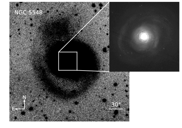
Figure 1.— Optical image of NGC 5548. A deep, $V$-band image taken with the Lijiang 2.4m telescope showing a long, tidal tail wrapping around the galaxy, indicative of a major merger $\sim 1$ Gyr ago. The inset panel highlights small-scale structure visible in a WFC3/F547M image obtained from the HST archives.

Early in 1987, using data from their three-year spectroscopic monitoring, Peterson et al. (1987) proposed that NGC 5548 contains a SMBHB to explain its asymmetric, varying H$\beta$ profiles. They roughly estimated that the binary period is of the order 110 yr. Using four decades of optical spectroscopic monitoring, we provide compelling evidence for a SMBHB in the galactic center of NGC 5548 based on more robust measurements of the period and binary orbital information.

The paper is organized as follows. In Section 2, we summarize the historical data available in the literature and our new observations taken in 2015 using the Lijiang 2.4m telescope and outline the procedures for homogeneous spectral measurements. In Section 3, we exploit the periodicity in the long-term variations of the continuum and H$\beta$ fluxes, and in the H$\beta$ profile changes. We find that these three periods are remarkably all in agreement within their uncertainties. Most importantly, the double-peaked H$\beta$ profiles shift and merge in a periodic manner. Together with the tidal tails of NGC 5548, these pieces of evidence indicate a SMBHB in its galactic center. In Section 4, we show that the lines of observations presented here can test existing interpretations for the periodicity in the continuum, H$\beta$ fluxes, and H$\beta$ profile changes, and the presence of a SMBHB is the most natural interpretation. We introduce a simple toy model of BLRs around a SMBHB and fit the H$\beta$ profiles to extract the orbital information in Section 5. We discuss the possible caveats of our SMBHB interpretation and future improvements in Section 6. The conclusions are summarized in Section 7.

Table 1Spectroscopic datasets of NGC 5548.

Dataset	Ref.	Observation Periods		Number of	Note
		JD (-2,400,000)	Year	Spectra
S07	1	41,420$-$52,174	1972 - 2001	814	Includes AGN Watch dataset
I95	2	47,169$-$49,534	1988$-$1994	23	$\cdots$
P08	3	51,020$-$53,065	1998$-$2004	22	$\cdots$
SDSS06	$\cdots$	53,859	2006	1	SDSS database
AGN05	4	53,431$-$53,472	2005	$\cdots$	Only H$\beta$ fluxes available
AGN07	5	54,180$-$54,333	2007	1	Mean spectrum
LAMP08	6	54,550$-$54,619	2008	1	Mean spectrum
M15	7	56, 490	2013	1	Only used for measuring H$\beta$ flux
This work	$\cdots$	57,030$-$57,236	2015	62	$\cdots$

References. — (1) Sergeev et al. (2007); (2) Iijima & Rafanelli (1995); (3) Popović et al. (2008); (4) Betnz et al. (2007); (5) Denney et al. (2010); (6) Bentz et al. (2009); (7) Mehdipour et al. (2015).

Table 2Datasets for the 5100 Å continuum fluxes of NGC 5548

Dataset	Ref.	Observation Periods		Number of	Aperture	$F_{\rm gal}$	Note
		JD (-2,400,000)	Year	Observations	(arcsec)
R95	1	39,941$-$45,174	1968$-$1982	17	$\cdots$	$\cdots$	$V$-band photometry
S07	2	41,420$-$52,174	1972$-$2001	814	$5.0\times 7.5$	$3.75\pm 0.38$	Partially overlaps with AGN Watch dataset
LD93	3	43,216$-$48,856	1977$-$1992	82	7.15	$7.08\pm 0.19$	$V$-band photometry
I95	4	47,169$-$49,534	1988$-$1994	23	$3.0\times 12.0$	$2.77\pm 0.18$	$\cdots$
AGN Watch	5	47,509$-$52,265	1989$-$2001	1548	$5.0\times 7.5$	$3.75\pm 0.38$	$\cdots$
A14	6	50,883$-$55,734	1998$-$2013	10	$\cdots$	$\cdots$	1350 Å fluxes
P08	7	51,020$-$53,065	1998$-$2004	22	$2.5\times 6.0$	$1.73\pm 0.17$	$\cdots$
K14	8	51,992$-$54,332	2001$-$2007	302	4.15	$4.21\pm 0.19$	$V$-band fluxes
R12	9	52,818$-$55,716	2003$-$2011	34	$\cdots$	$\cdots$	$V$-band photometry
AGN05	10	53,431$-$53,472	2005	40	$5.0\times 12.75$	$4.34\pm 0.43$	$\cdots$
SDSS06	$\cdots$	53,859	2006	1	1.5	$1.16\pm 0.14$	SDSS database
AGN07	11	54,180$-$54,333	2007	220	$5.0\times 12.0$	$4.27\pm 0.43$	$\cdots$
LAMP08	12	54,509$-$54,617	2008	57	$4.0\times 9.4$	$3.54\pm 0.35$	$\cdots$
AGN12	13	55,932$-$56,048	2012	90	$5.0\times 15.0$	$4.45\pm 0.44$	$\cdots$
E15	14	56,431$-$56,824	2013$-$2014	409	5	$5.07\pm 0.19$	$V$-band fluxes
This work	$\cdots$	57,030$-$57,236	2015	62	$2.5\times 8.5$	$2.04\pm 0.17$	$\cdots$

References. — (1) Romanishin et al. (1995); (2) Sergeev et al. (2007); (3) Lyutyi & Doroshenko (1993); (4) Iijima & Rafanelli (1995); (5) Peterson et al. (2002); (6) Arav et al. (2014); (7) Popović et al. (2008); (8) Koshida et al. (2014); (9) Roberts & Rumstay (2012); (10) Betnz et al. (2007); (11) Denney et al. (2010); (12) Bentz et al. (2009); (13) Peterson et al. (2013); (14) Edelson et al. (2015).

2. Observations of NGC 5548 and data processing

2.1. New observations in 2015

We made spectroscopic and photometric observations of NGC 5548 from January 7 to August 1, 2015, using the Lijiang 2.4m telescope, located in Yunnan Province, China, operated by Yunnan Observatories. The Yunnan Faint Object Spectrograph and Camera (YFOSC) is equipped with a back-illuminated 2048$\times$4608 pixel CCD covering a field-of-view of $10^{\prime}\times 10^{\prime}$. The photometric observations use a Johnson $V$ filter. Details of the telescope, YFOSC, observational setup, and data reduction can be found in Du et al. (2014). To achieve accurate absolute and relative flux calibration, we took advantage of the long-slit capability of YFOSC and simultaneously observed a nearby comparison star as a reference standard. Absolute flux calibration of the comparison star is obtained using observations of spectrophotometric standards during nights of good weather conditions. Given the seeing of the observations ($1.0^{\prime\prime}-2.5^{\prime\prime}$), the slit was fixed at a projected width of $2.5^{\prime\prime}$. The grism provides a resolution of 92 Å ${\rm mm^{-1}}$ (1.8 Å per pixel) and covers the wavelength range $3800-7200$ Å. The spectra were extracted using a uniform window of $8.5^{\prime\prime}$. In total, we obtained 61 photometric observations and 62 spectroscopic observations, with typical exposures of 5 and 20 min, respectively. The detailed dataset and reverberation analysis will be presented in a separate paper (Lu et al. 2016).

To obtain a deep image of NGC 5548, we aligned and stacked all the photometric data, resulting in a long-exposure image with a total integration time of 3950 s. Figure 1 shows the final stacked image, in which the bending long tail, first detected by Schweizer & Seitzer (1988), is clearly seen. We also superpose a WFC3/F547M image obtained from the Hubble Space Telescope (HST) archives to highlight small-scale structure of NGC 5548.

2.2. Historical data and construction of a homogeneous database

NGC 5548 has been observed many times individually (e.g., Iijima & Rafanelli 1995; Shapovalova et al. 2004; Sergeev et al. 2007; Popović et al. 2008), and 16 monitoring campaigns have been devoted to reverberation mapping of the H$\beta$ emission line (e.g., Peterson et al. 2002; Betnz et al. 2007; Bentz et al. 2009; Denney et al. 2010). In Tables 1 and 1, we compile spectroscopic and photometric data available in the literature and list the corresponding references. Appendix A.1 gives the detailed information for the spectroscopic data sources. We also collected $V$-band photometric data and UV 1350 Å data. Appendix A.2 shows how to convert continuum fluxes from these bands to 5100 Å. Because the aperture sizes are different among the data sources, we subtract the host galaxy contribution from the 5100 Å fluxes as described in the next section.

The database constitutes a variety of sources with different aperture sizes, resolution, and wavelength and flux calibration; therefore, it is important to compile and calibrate them in a systematic fashion. Fortunately, most spectroscopic data sources listed in Tables 1 and 1 were calibrated uniformly, in a manner similar to that employed for the AGN Watch project, based on a constant [O III] flux (see below). This allows us to directly use their published 5100 Å continuum and integrated H$\beta$ fluxes. However, for H$\beta$ profiles, extra calibration is required because the reference [O III] profiles among the data sources are generally different in spectral resolution and wavelength calibration.

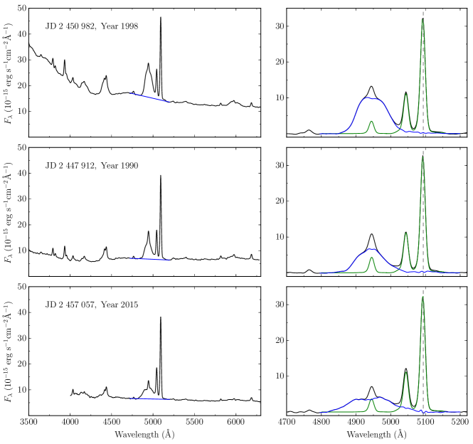
Figure 2.— Three illustrative examples for the spectral decomposition. Left panels: calibrated spectra, showing the blue straight line used to subtract the pseudo continuum. Right panels: continuum-subtracted spectra around H$\beta$ line in the observed frame (see the text for details), where green line represents the narrow-line components (the narrow H$\beta$ and [O III] doublet), blue line represents the broad H$\beta$ component, and grey dashed line represents the location of [O III] $\lambda 5007$. Top two panels show the spectra at high and low state ($F_{\rm 5100}=10.2,3.1\times 10^{-15}~{}{\rm erg\,s^{-1}\,cm^{-2}\,\text{\AA}^{-1}}$), respectively, from the AGN Watch project, and bottom panel shows a spectrum from our new observations ($F_{\rm 5100}=3.0\times 10^{-15}~{}{\rm erg\,s^{-1}\,cm^{-2}\,\text{\AA}^{-1}}$).

The majority of the spectroscopic data comes from Sergeev et al. (2007) (S07; see Table 1), who included archival data from 1972–1990 and high-quality data from the AGN Watch project from 1989–2001. The authors calibrated all their spectra based on the usual assumption that the narrow [O III] $\lambda 5007$ line does not vary with time (van Groningen & Wanders 1992) and further inter-calibrated the spectra to account for aperture effects (Peterson et al. 1995; Li et al. 2014). Inter-calibration is necessary because the narrow-line region of NGC 5548 is spatially resolved so that different apertures admit different amounts of light from the narrow-line region. The absolute flux of [O III] was set to $F([\text{{O~{}III}}])=5.58\times 10^{-13}\,{\rm erg\,s^{-1}\,cm^{-2}}$ (Peterson et al. 2002). Sergeev et al. measured the 5100 Å continuum and decomposed the broad H$\beta$ profiles with the narrow-line component subtracted, and kindly made them available to us. We directly use these data for our analysis. We align the spectra from other data sources with those of S07, using the same data calibration processing. To be specific, by comparing the [O III] $\lambda 5007$ line with respect to the dataset of S07, we correct for the differences of the other datasets in spectral resolution, wavelength and flux calibration. We then perform inter-calibration for data sources I95 and P08 in Table 1 by comparing the measurements of 5100 Å continuum and H$\beta$ fluxes with those from S07 and AGN Watch that are closely spaced within a time interval of 20 days. For data sources that do not overlap with the other sources (e.g., those after 2004 in Table 1), provided that the adopted aperture is large enough (e.g., circular aperture radius $\lower 2.0pt\hbox{$\,\buildrel\scriptstyle>\over{\scriptstyle\sim}\,$}3^{\prime\prime}$), all the narrow-line flux should be enclosed so that inter-calibration is no longer needed; otherwise, we use the surface-brightness distribution of narrow [O III] $\lambda 5007$ derived by Peterson et al. (1995) to determine a correction factor. It turns out that only the data from source SDSS06 and from this work require a correction.

Note that the AGN Watch project published their full data for 5100 Å continuum and integrated H$\beta$ fluxes in Peterson et al. (2002), and Sergeev et al. (2007) included only the high-quality spectra of the AGN Watch project in their compilation. Therefore, these two data sources partially overlap. For the overlapping portion, when analyzing the light curves of the 5100 Å and integrated H$\beta$ fluxes, we use the full data from the AGN Watch project; whereas when analyzing the H$\beta$ profiles, which requires higher quality data, we only use the data from Sergeev et al. (2007).

2.3. Spectral measurements

For the purpose of homogeneous spectral measurements, we measure the 5100 Å flux density and decompose the broad H$\beta$ line using the same standard procedure as in Sergeev et al. (2007). Specifically, we measure the 5100 Å continuum flux $F_{5100}$ as the average flux density in a 50 Å-wide wavelength range centered on 5100 Å in the rest frame. The uncertainty is set by the standard deviation of fluxes in the same wavelength range. To correct for host galaxy contribution to the 5100 Å continuum, we use the $V$-band aperture magnitudes of the host galaxy derived by Romanishin et al. (1995). The $V$-band magnitude is converted into 5100 Å continuum flux ($F_{5100}$) by assuming that NGC 5548 has a galaxy spectral template similar to that of M32. This leads to $F_{5100}=3.4\times 10^{-15}\,{\rm erg\,s^{-1}\,cm^{-2}\,\text{\AA}^{-1}}$ for a $V$-band magnitude of 14.99 (Romanishin et al. 1995). We compared our host galaxy corrections with those given in Peterson et al. (2013) and find that the differences are generally smaller than 10%.

To decompose the broad H$\beta$ line, we subtract the underlying continuum, the narrow H$\beta$ component, and the [O III]$~{}\lambda\lambda$4959, 5007 doublet, which severely blends with H$\beta$ during the low-flux states of NGC 5548. Since the spectra have been calibrated to a common [O III] $\lambda 5007$ flux, the doublet can be subtracted uniformly by creating a template. We make use of the [O III]-doublet template of Sergeev et al. (2007), in which the doublet lines was assumed to have the same profile with an intensity ratio of 2.93. Following the approach described in Sergeev et al. (2007), we first remove the continuum by subtracting a straight line interpolated between two 40 Å-wide windows centered on 4640 Å and 5110 Å in the rest frame. We then remove the [O III] doublet using the template and remove the narrow H$\beta$ component using the same template but adjusting its position and intensity to achieve the smoothest broad-line H$\beta$ profile. The obtained flux ratio of narrow H$\beta$ to [O III] $\lambda 5007$ generally ranges from 0.10 to 0.15, consistent with the previous determinations (Peterson et al. 2004; Sergeev et al. 2007). After obtaining the broad H$\beta$ line, its integrated flux is calculated over a uniform wavelength window 4714–4933 Å in the rest frame, as in Peterson et al. (2002).

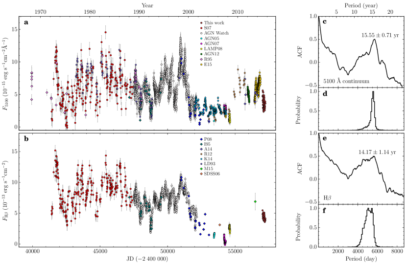
Figure 3.— Period determination from the light curves in (a) 5100 Å continuum and (b) H$\beta$. Data sources are labelled and explained in Appendix A and Tables 1 and 1. The ACF and distribution of the peak period for the continuum are shown in panels (c) and (d), and for H$\beta$ in panels (e) and (f).

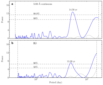
Figure 4.— Lomb$-$Scargle periodograms of the light curves in (a) 5100 Å continuum and (b) H$\beta$ fluxes (blue lines), using the procedure given by Press et al. (1992). Solid grey lines show the periodograms of the data window, which help uncover spurious signals caused by the sampling; none is seen. Dashed vertical lines represent the Nyquist frequency and the time span of the light curve, respectively, and dashed horizontal lines represent the confidence levels.

It is worth stressing that in the decomposition procedure described above, we ignore Fe II blends and the broad He II $\lambda 4686$ emission line. In addition, the absorption of host galaxy at H$\beta$ line will also deform the obtained H$\beta$ profiles. In Appendix B, we perform a simple test to show that host galaxy contamination is unimportant on the H$\beta$ profiles when the flux ratio between the central AGN and the host galaxy at 5100 Å is larger than $F_{\rm AGN}/F_{\rm gal}\approx 0.5$; otherwise, the host galaxy contamination leads to apparent double peaks in the H$\beta$ profile. The resulting changes in the integrated H$\beta$ fluxes are less than 10% for $F_{\rm AGN}/F_{\rm gal}\lower 2.0pt\hbox{$\,\buildrel\scriptstyle>\over{\scriptstyle\sim}\,$}0.2$, which is generally satisfied in our database (see Figure 3). Therefore, we use all the data for analyzing the light curves, but exclude those spectra with small $F_{\rm AGN}/F_{\rm gal}$ for analyzing H$\beta$ profiles. We adopt a lower limit of $F_{\rm AGN}/F_{\rm gal}\approx 0.7$ to be conservative. The spectroscopic data sources AGN05, AGN07, and LAMP08, together with several spectra in other data sources—in total 85 out of 924 spectra—are finally discarded.

Fe II emission is relatively weak in NGC 5548 (e.g., Wamsteker et al. 1990; Vestergaard & Peterson 2005; Denney et al. 2009; Mehdipour et al. 2015). Vestergaard & Peterson (2005) selected 73 spectra of NGC 5548 spanning 13 years of the AGN Watch project and quantitatively showed that, on average, the flux ratio of optical Fe II over the range 4250–5710 Å (rest-frame) to broad H$\beta$ line is 0.66. The strength of Fe II emission in the H$\beta$ window is fairly small and is thus expected to have little effect on the broad H$\beta$ profile.

The broad He II $\lambda 4686$ line blends with the blue wing of H$\beta$ (Bottorff et al. 2002). Denney et al. (2009) studied exhaustively the contamination of He II $\lambda 4686$ on H$\beta$ for NGC 5548, again using the spectra from the AGN Watch project. Their results showed that although deblending He II slightly increases the flux of the far blue wing of H$\beta$, its influence on the H$\beta$ line width (in term of full width at half maximum) is safely negligible (see their Figures 16 and 19). We also expect contamination from He II $\lambda 4686$ to be unimportant.

In Figure 2, we show three illustrative examples for our spectral decomposition, with the first two spectra from the AGN Watch project, taken during high and low state, respectively, and the other one from our new observations. As can be seen, it is safe to ignore the Fe II emission and the broad He II line for our present purposes.

3. Periodicity of long-term variations

The optical photometric and spectroscopic data cover a time span of over four decades. Figures 3a and 3b plot light curves of the 5100 Å continuum and H$\beta$ fluxes, respectively. Appendix A shows all the H$\beta$ profiles. It is obvious at first glance that light curves of both the 5100 Å continuum and H$\beta$ appear periodic. Below we first summarize the properties of the long-term variations in the continuum, H$\beta$ flux, and as well as H$\beta$ profile, and then explore the periodicity in these variations.

3.1. Properties of long-term variations

The continuum and H$\beta$ light curves of NGC 5548 exhibit three types of variations:

1. Short-term fluctuations of a factor of $1.5-2$ at any epoch, which could be driven by local instabilities of the accretion disk(s). They are well-modeled as a damped random walk (Kelly et al. 2009; Li et al. 2013b), with a characteristic timescale that depends on the optical luminosity. The average timescale over 16 monitoring campaigns is about $\tau_{c}\approx 150$ days (Li et al. 2013b). This kind of variations is used for measurements of H$\beta$ reverberation mapping to reveal the BLR structure and dynamics. The H$\beta$ flux variations lag from 5 to 30 days behind the continuum variations, depending on the continuum flux state (e.g., Bentz et al. 2013).

2. Long-term variability by a factor of $\sim 10$ on a timescale of 10 yr, which, according to our analysis, appears to be periodic and governed by the orbital motion of a SMBHB. This type of variability has the largest amplitude.

3. Abrupt changes by a factor up to $3-4$, such as the large dip in the 5100 Å continuum in 1981$-$1982, in 1996, and in 1997$-$1998, and the strong flare in 1972$-$1973 and 1998–1999. The causes for these irregular changes are unknown. Such patterns of abrupt changes is very similar to that seen in OJ 287, which has long been suspected to host a SMBHB system (e.g., Sundelius et al. 1997; Valtonen et al. 2008).

The broad H$\beta$ line of NGC 5548 generally always has a complex, asymmetric profile (e.g., Shapovalova et al. 2004), which has been suggested to be caused by a superposition of several physically distinct components that vary with time (e.g., Peterson 1987; Sergeev et al. 2007). From the four decades of record, we can generally identify four types of H$\beta$ profiles:

1. An asymmetric shape during some high states.

2. A very broad and highly asymmetric shape with a width of $\sim 10^{4}\,\rm km~{}s^{-1}$ during low states.

3. A double-peaked shape during some intermediate-luminosity states.

4. A highly asymmetric, shape dominated by a blue component seen around 1972 and 1985.

As we will show below, the profile variations are consistent with orbital motion of two BLRs associated with a SMBHB system. The period inferred from the profile changes agrees with the periods observed in the 5100 Å  continuum and H$\beta$ flux series.

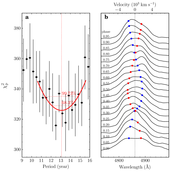
Figure 5.— (a) $\chi_{\rm p}^{2}$ versus period from the epoch-folding scheme to determine the period ($T_{P_{\rm H\beta}}$) of H$\beta$ profile variations, in which the phase width is set to $\Delta\phi=150$ days (see Section 3.3 for details). We fit the $\chi_{\rm p}^{2}-T_{P_{\rm H\beta}}$ relation with a second-order polynomial and determine the period by the minimum of the polynomial, which yields $T_{\rm P_{H\beta}}=(13.10\pm 0.88)$ yr. The uncertainty is determined by $\Delta\chi_{\rm p}^{2}=3.1$, which corresponds to a confidence level of $68.3\%$ (“$1\sigma$”). (b) Folded H$\beta$ profile series with phases for a complete cycle using the mean period 14.14 yr. To guide the eye, blue and red points are superposed to show the line-of-sight velocities of the black hole pair from our SMBHB model (see Section 5).

Table 3Summary on the observed periods of 5100 Å continuum flux, H$\beta$ flux, and H$\beta$ profile in NGC 5548

Period	Meaning	Value (yr)	Method
$T_{\rm 5100}$	Period of 5100 Å continuum	$15.55\pm 0.71$	ACF method
		$14.50$	Lomb-Scargle periodogram
$T_{\rm F_{\rm H\beta}}$	Period of integrated H$\beta$ fluxes	$14.17\pm 1.14$	ACF method
		$13.39$	Lomb-Scargle periodogram
$T_{\rm P_{H\beta}}$	Period of H$\beta$ profiles	$13.10\pm 0.88$	Epoch-folding scheme
Mean	$\cdots$	$14.14\pm 0.87$	$\cdots$

Note. — The uncertainty of the mean period is set by the standard deviation of the five observed periods.

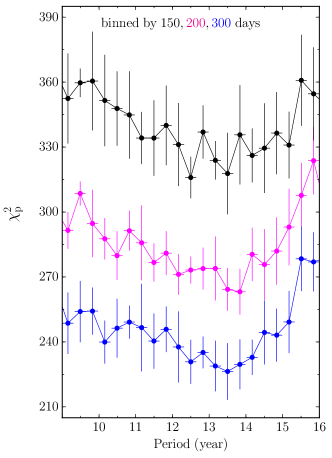
Figure 6.— $\chi_{\rm p}^{2}$ versus period for different phase widths ($\Delta\phi=150,200,300$ days) of the epoch-folding scheme (see Section 3.3 for details). As can be seen, the period of H$\beta$ profile variations $T_{\rm P_{H\beta}}$, determined from the minimum $\chi_{\rm p}^{2}$, is insensitive to the choice of $\Delta\phi$.

3.2. 5100 Å continuum and H$\beta$ line fluxes

We applied the auto-correlation function (ACF) technique to identify the periods of continuum and emission-line flux variations. We use the interpolation cross-correlation function method of Gaskell & Peterson (1987) to calculate the ACFs and the model-independent FR/RSS Monte Carlo method described by Peterson et al. (1998) to determine the associated uncertainties. The period is determined by the centroid of the ACF around its peak (excluding the zero peak) above a threshold of 80% of the peak value (Peterson et al. 1998). To suppress the short-term fluctuations in the light curves (see Section 3.1), we bin the light curves with an interval of 150 days, the characteristic timescale of fluctuations. The uncertainties of points in the newly binned series are assigned as follows: we first calculate the mean standard deviation of the whole light curve, and then compare it with the standard deviations of each bin and set the associated uncertainty to be the maximum one. Such a choice can account for the sparse sampling in some periods (e.g., around 2010) and avoid unrealistic weights of these measurements in calculating the ACFs.

Figures 3c$-$3f show the ACF results and period distributions from standard Monte Carlo simulations (Peterson et al. 1998). We detect highly significant peaks in the ACFs of the 5100 Å continuum and H$\beta$ light curves that correspond to periods of $T_{5100}=15.55\pm 0.71$ yr and $T_{\rm F_{\rm H\beta}}=14.17\pm 1.14$ yr, respectively, where the uncertainties are determined by the period distributions with a 68.3% confidence level (“1$\sigma$”). We note that $T_{\rm F_{\rm H\beta}}\approx T_{5100}$, which is likely a direct consequence of photoionization of the BLR by the central continuum.

We also apply the Lomb-Scargle normalized periodogram (e.g., Press et al. 1992) to test for periodicity in the light curves. Again, the light curves are binned with an interval of 150 days. Figure 4 shows the Lomb-Scargle periodograms over a period range limited by the average Nyquist frequency and the time span of the light curve, using the procedure given by Press et al. (1992) . The periodogram of the 5100 Å continuum peaks at 14.50 yr with a confidence level $>99.9$%; for the H$\beta$ fluxes, it peaks at 13.39 yr with a confidence level $>90$%. Here, the confidence level represents the probability that the data contain a periodicity and can be tested by the statistic $1-p$, where $p$ is the false alarm probability of the null hypothesis (Press et al. 1992). To exclude spurious signals caused by the sampling, we also plot the periodograms of data window in Figure 4. As can be seen, the periodicity cannot arise from the sampling. The obtained periods are generally consistent with those from the ACF method.

Although there exists alternative explanations, a periodic variability in time series of flux measurements is widely used to search for SMBHB candidates (e.g., Graham et al. 2015a, b; Liu et al. 2015b). The best-known candidate is OJ 287, which exhibits outburst peaks every $\sim 12$ years (Valtonen et al. 2008). Recently, Graham et al. (2015b) performed a systematic search for periodic light curves in quasars covered by the Catalina Real-time Transient Survey and obtained a sample of more than 100 candidates. However, as the authors note, more spectroscopic observations are required to verify the SMBHB hypothesis. Nevertheless, the periodicity of the H$\beta$ and continuum long-term variations suggests that NGC 5548 may host a SMBHB system. Compared with the above candidates, NGC 5548, at a distance of $\sim 75$ Mpc, is to date one of the nearest objects with periodic behavior. Another nearby case is NGC 4151 at $\sim 14$ Mpc ($z=0.003319$), which, interestingly, was also found to have a similar period of $\sim 15$ yr in flux variations (Pacholczyk et al. 1983; Guo et al. 2006). The SMBHB hypothesis in NGC 4151 was subsequently reported by Bon et al. (2012) based on an analysis of the H$\alpha$ emission line. Below we use the extensive spectroscopic monitoring database over four decades (much longer than the time span of the database for NGC 4151) to provide more evidence for a SMBHB in NGC 5548.

3.3. H$\beta$ profiles and epoch-folding scheme

The H$\beta$ profiles of NGC 5548 generally show two peaks superposed on a very broad wing, however, during most epochs the double peaks are indistinct and not well-separated. This prevents us from unambiguously testing the SMBHB model as in previous works by directly comparing the velocity changes of the double peaks with the orbital motion of a SMBHB model (e.g., Eracleous et al. 1997). Notwithstanding, over time the H$\beta$ profiles clearly exhibit systematic variations: the peaks shift and vary, plausibly periodically, on a long timescale (see the series of spectra over four decades in Appendix A). As illustrated in Appendix B, the variations cannot be due to host galaxy contamination.

H$\beta$ has been monitored over more than two cycles of the orbital period of $\sim 14$ yr, long enough to use the epoch-folding scheme to test for periodicity in the line profile variations. Our epoch-folding scheme is as follows. Supposing a trial period $T_{\rm P_{H\beta}}$, we group the temporal series of the normalized H$\beta$ profiles into $\left\{\left[\left(t_{N}-t_{0}\right)/T_{\rm P_{H\beta}}\right]+1\right\}$ uniformly spaced cycles, where the brackets of $[B]$ indicate the integral part of number $B$, and $t_{0}$ and $t_{N}$ are the starting and ending times of the series, respectively. In each cycle, we divide the series into $N_{\phi}=T_{\rm P_{H\beta}}/\Delta\phi$ uniformly spaced phases by a phase width $\Delta\phi$. For an H$\beta$ spectrum at time $t_{j}$, it will be grouped into the phase of $\left\{(t_{j}-t_{0})/T_{\rm P_{H\beta}}-[(t_{j}-t_{0})/T_{\rm P_{H\beta}}]\right\}$ in the cycle of $\left\{\left[\left(t_{j}-t_{0}\right)/T_{\rm P_{H\beta}}\right]+1\right\}$. In the $k$th-phase of the $i$th-cycle, we calculate the averaged spectrum $\bar{F}_{\lambda}^{i,k}$ and the standard deviation $\sigma_{\lambda}^{i,k}$, and then calculate the averaged spectrum $\widehat{\bar{F}}_{\lambda}^{k}$ of the $k$th-phase over all the cycles. Finally, we compare the differences of the averaged spectra in the same phase of different cycles by defining a statistical quantity

$$\chi_{\rm p}^{2}(T_{\rm P_{H\beta}})=\frac{1}{N_{\phi}}\sum_{k}\frac{1}{N_{k}-1}\sum_{N_{\lambda}}\sum_{i}\left(\bar{F}_{\lambda}^{i,k}-\widehat{\bar{F}}_{\lambda}^{k}\right)^{2}\Bigg{/}\left(\sigma_{\lambda}^{i,k}\right)^{2},$$ (1)

where $N_{\lambda}$ is the wavelength number of H$\beta$ profiles and $N_{k}$ is the number of cycles for the $k$th-phase. The minimum of $\chi_{\rm p}^{2}$ means that the H$\beta$ lines with a time difference $T_{\rm P_{H\beta}}$ have systematically similar profiles. In other words, the H$\beta$ profiles have periodic variations with a period $T_{\rm P_{H\beta}}$. It is worth stressing the two following points: (1) the H$\beta$ profiles are normalized to avoid the influence of the periodicity in the integrated H$\beta$ fluxes; (2) the random fluctuations of the profiles in the $k$th-phase are suppressed by averaging the spectra in the calculation of $\chi_{\rm p}^{2}$.

For the datasets of NGC 5548, the wavelength number is large ($N_{\lambda}\gg 1$). It can be shown that the quantity $\chi_{\rm p}^{2}$ approximately follows a normal distribution with a mean of $N_{\lambda}$ and a standard deviation of $\sqrt{2N_{\lambda}/(N_{k}-1)N_{\phi}}$. We determine the confidence interval of $T_{\rm P_{H\beta}}$ by $\Delta\chi_{\rm p}^{2}=3.1$, which corresponds to a 68.3% confidence level (“$1\sigma$”). In our calculations, we adopt the phase width $\Delta\phi=150$ days. We use a second-order polynomial to fit the $\chi_{\rm p}^{2}-T_{\rm P_{H\beta}}$ relation and determine the period by the minimum of the polynomial. Figure 5a shows that $\chi_{\rm p}^{2}$ reaches a minimum at $T_{\rm P_{H\beta}}=(13.10\pm 0.88)$ yr, which indicates the period of H$\beta$ profile variations. In Figure 6, we test the dependence of $\chi_{\rm p}^{2}$ on the phase width $\Delta\phi$ and find that the resulting periods from the minimum of $\chi_{\rm p}^{2}$ are insensitive to the choice of $\Delta\phi$.

Since the 5100 Å continuum of NGC 5548 varies periodically, we expect that the line width of broad H$\beta$ line should also follow such a temporal variation pattern ($\sigma({\rm H\beta})\propto F_{\rm con}^{-1/4}$), simply from the well-established relationship between the BLR size and AGN 5100 Å luminosity (the $R_{\rm BLR}-L$ relation; e.g., Bentz et al. 2013) and the virial relation of the BLR motion (e.g., Peterson & Wandel 1999; Peterson et al. 2004; Simic & Popovic 2016). This will contribute to the periodicity of H$\beta$ profiles seen in the above epoch-folding scheme. In Appendix C, we perform a simple simulation test to show that the periodicity in variations of the H$\beta$ profiles does not entirely result from such a dependence of the H$\beta$ line width on the continuum.

To clarify long-term variations of the two peaks, we folded the spectra over four decades in light of phases using the mean period 14.14 yr (see Table 3). Figure 5b shows the folded spectra series with phases for one complete cycle. The two peaks of H$\beta$ profiles seem to shift in an opposite direction. To guide the eye, we also superpose the line-of-sight velocities of the black hole pair (red and blue points) inferred from our SMBHB BLR model, as described below.

Within uncertainties, the three periods of variability, namely that of the H$\beta$ profile, H$\beta$ flux, and continuum flux, are all in agreement, i.e., $T_{\rm P_{H\beta}}\approx T_{\rm F_{\rm H\beta}}\approx T_{5100}$. Combining with the tidal imprints of a major merger event in the morphology of the host galaxy, this constitutes very compelling spectroscopic evidence for the presence of a SMBHB in NGC 5548.

NGC 5548 contains a classical bulge (Ho & Kim 2014) with a central stellar velocity dispersion of $\sigma_{*}=195\pm 13\,\rm km~{}s^{-1}$ (Woo et al. 2010). This yields a (total) black hole mass of $\log\left(M_{\bullet}/M_{\odot}\right)=8.44\pm 0.14$ from the $M_{\bullet}-\sigma_{*}$ relation (Kormendy & Ho 2013). Using this mass as the total mass of the SMBHB system and the mean observed period as the (redshifted) orbit period (Table 3), we determine the semi-major axis of the orbit from Kepler’s third law, $a_{\bullet}=21.73\pm 2.43$ light-days (Table 4).

4. Confronting alternative interpretations

Besides the SMBHB model, there are several alternative models/interpretations for the periodicity in the light curves and line profiles; however, most cannot simultaneously account for all of the evidence in NGC 5548. Double-peaked profiles of broad emission lines quite often appear in low-luminosity AGNs (Eracleous et al. 1995; Ho et al. 2000; Strateva et al. 2003; Lewis et al. 2010), and can be understood in the context of the radiatively inefficient accretion flow structure of AGNs accreting at highly sub-Eddington rates (Ho 2008). NGC 5548 has an Eddington ratio $\lower 2.0pt\hbox{$\,\buildrel\scriptstyle>\over{\scriptstyle\sim}\,$}10^{-2}$ (Ho & Kim 2014); it does not belong to the class of low-accretion rate systems. The central (or binary) black hole mass of NGC 5548, $M_{\bullet}\approx 10^{8}M_{\odot}$, is quite secure, both from reverberation mapping and from the bulge stellar velocity dispersion (Ho & Kim 2015). Reverberation mapping finds the H$\beta$ BLR radius lies in the range $5-30$ light-days (Bentz et al. 2013), corresponding to $R_{\rm H\beta}\sim 10^{3}R_{\rm g}$, where $R_{\rm g}=GM_{\bullet}/c^{2}$ is the gravitational radius. These facts, together with the periodicity, allow us to evaluate the interpretations listed below.

4.1. Disk model

Double-peaked broad emission lines are commonly modeled as disk emission. We dismiss the disk model for NGC 5548 based on the following arguments. A simple circular disk model can be easily ruled out because, due to relativistic boosting, the blue peak should always be stronger than the red peak, clearly contrary to what is observed. In the precessing eccentric disk model (Eracleous et al. 1995), the precession period due to the relativistic advance of the pericenter can be expressed as (Weinberg 1972)

$$T_{\rm prec}=\frac{2\pi}{3}\frac{1+e}{(1-e)^{3/2}}\frac{GM_{\bullet}}{c^{3}}R^{5/2}=10^{3}\frac{1+e}{(1-e)^{3/2}}m_{8}r_{3}^{5/2}\,{\rm yr},$$ (2)

where $e$ is the eccentricity, $m_{8}=M_{\bullet}/10^{8}\,M_{\odot}$, and $r_{3}=R_{\rm H\beta}/10^{3}\,R_{\rm g}$. The term $(1+e)/(1-e)^{5/2}$ is always larger than 1, and as a result the precession period is $>10^{3}$ yr, making this model implausible.

For the case of precessing spiral arms in a disk (Storchi-Bergmann et al. 2003), an upper limit bound to the pattern period is set by the sound-crossing timescale, $T_{\rm s}=R/c_{\rm s}=66m_{8}r_{3}T_{5}^{-1/2}\,{\rm yr}$, where the disk temperature $T_{5}=T/10^{5}$ K, beyond which thermal dissipation will smear out the spiral arms. Numerical simulations by Laughlin & Korchagin (1996) show that the pattern speed is several times to an order of magnitude larger than the dynamical timescale, $T_{\rm dyn}\sim(R^{3}/GM_{\bullet})^{1/2}=0.5m_{8}r_{3}^{3/2}$ yr. The pattern period is between $T_{\rm dyn}$ and $T_{\rm s}$, which in general can match the observed period. Given the many unconstrained free parameters in the spiral-arm disk model, with sufficient tuning it certainly should be able to reproduce the observed H$\beta$ profiles. However, this model takes no account of the periodic variations in 5100 Å continuum and H$\beta$ fluxes.

It is possible the thermal instability of the accretion disk leads to repeat outbursts of accretion onto the black hole and gives rise to periodic continuum variations, but this generally occurs on a much long timescale of the order of $10^{3}-10^{5}$ yr (e.g., Mineshige& Shields 1990; Hameury et al. 2009; Janiuk & Czerny 2011). Even if the instability were to develop only in a part of the disk and the continuum variations are modulated by the disk rotation, the amount of the modulation (i.e., the Doppler boosting) in the regions that produce the 5100 Å continuum (at $\sim 10^{3}R_{\rm g}$ with a period of $\sim 14$ yr) is insufficient for the observed large amplitude (see also Section 4.3). Another possibility is that the spiral arms may trigger periodic accretion onto the central black hole and thereby may result in the periodic variability in the continuum (Y. Shen, private communications). Chakrabarti & Wiita (1993) studied the variations in emission from accretion disks with spiral shocks and tended to use such a model to explain the micro-variability in AGNs. It is unclear yet if spiral arms can drive the large-amplitude variations observed in NGC 5548.

4.2. Precessing jet model

The expected precession period for a single SMBH is given by

$$P=10^{9.25}\alpha^{48/35}a^{5/7}m_{8}^{1/7}\left(\frac{\dot{M}_{\bullet}}{10^{-2}~{}M_{\odot}{\rm yr}^{-1}}\right)^{-6/5}~{}{\rm yr},$$ (3)

where $\alpha$ is the viscosity parameter, $a$ is black hole spin, and $\dot{M}_{\bullet}$ is the mass accretion rate (Lu & Zhou 2005). This period is typically much longer than the observed period unless $a$ approaches extraordinarily close to 0. On the other hand, the radio-loudness parameter of NGC 5548’s nucleus is $\log{\cal R}=1.24$ (Ho & Peng 2001), meaning that it is only marginally radio-loud. The global spectral energy distribution for NGC 5548 also suggests that the 5100 Å continuum predominantly stems from an accretion disk (Chiang & Blaes 2003; Mehdipour et al. 2015). We can thus rule out with certainty that the periodicity originates from a precessing jet.

4.3. Hot spot model

In this model, a bright hot spot embedded in the accretion disk orbits around the central black hole and produces an excess, time-varying component in line emission (e.g., Newman et al. 1997; Jovanović et al. 2010). There are no physical constraints for most of the free parameters of the model (e.g., amplitude, width, and location of the spot, etc.). Fine-tuning some of them, one can generally simulate complicated H$\beta$ profiles. However, as in the disk models, this model does not account for the periodic variations in 5100 Å continuum and H$\beta$ fluxes. From the reverberation-mapping observations of the H$\beta$ line (Bentz et al. 2013), we know that the orbit size of the hot spot is $R_{\rm spot}\approx 10^{3}R_{\rm g}$, which is located at the outer region of the disk. Assuming a Keplerian orbit, the velocity of the spot is $\beta=V_{\rm spot}/c\approx 0.03\,(R_{\rm spot}/10^{3}R_{\rm g})^{-1/2}$. The resulting Doppler boosting factor

$$\delta=\frac{1}{\varGamma(1-\beta\cos\varphi\cos i)}\approx 1+\beta\cos\varphi\cos i,$$ (4)

is confined to a range $1\pm 0.03$, where $\varGamma=(1-\beta^{2})^{-1/2}$ is the Lorentz factor, $i$ is the orbital inclination angle, and $\varphi$ is the phase angle. If this model works in NGC 5548, the amount of Doppler beaming is too small to produce the observed variability amplitude of the integrated H$\beta$ fluxes. On the other hand, the disk instability predicted by existing models also cannot appropriately account for the large amplitude variation of the 5100 Å continuum (Section 4.1). Taken together, these facts do not support the hot spot model.

4.4. Warped accretion disk model

A warped accretion disk will precess around the central black hole and eclipse some parts of the continuum (e.g., Pringle 1996), leading to periodic variations in the continuum. There are two types of warps in disks surrounding single SMBHs: irradiation-induced warps by a central radiation source (Pringle 1996), and Lense-Thirring torque-induced warps by a spinning black hole (e.g., Bardeen & Petterson 1975; Martin et al. 2007).

For the irradiation-induced warps, the condition of warp instability is

$$\frac{R_{\rm warp}}{R_{\rm g}}>16\pi^{2}\eta^{2}\epsilon^{-2},$$ (5)

where $\eta$ is the ratio of the viscosity in the vertical and azimuthal directions and $\epsilon$ is the accretion efficiency. This gives $R_{\rm warp}\sim 10^{4}R_{\rm g}$ if we set $\eta\approx 1$ and $\epsilon\approx 0.1$. The precession timescale is

$$P_{\rm prec}=\frac{12\pi c\Sigma R_{\rm warp}^{3}\Omega_{\rm Kep}}{L}\approx\frac{12\pi cM_{\rm disk}R_{\rm warp}\Omega_{\rm Kep}}{L},$$ (6)

where $c$ is the speed of light, $\Sigma$ is the surface density, $\Omega_{\rm Kep}$ is the orbital angular velocity, and $M_{\rm disk}$ is the mass of the warped disk (Pringle 1996; Strochi-Bergmann et al. 1997). If we adopt $M_{\rm disk}\sim(10^{-2}-10^{-3})M_{\bullet}$ and $L=10^{43}\,{\rm erg~{}s^{-1}}$, the period is on the order of $10^{6-7}$ yr, much longer than the observed period of $\sim 14$ yr.

The Lense-Thirring torque-induced warps occur when a disk is inclined with respect to the spin axis of the central black hole (e.g., Martin et al. 2007). The warp radius is typically $300R_{\rm g}$, depending on the black hole spin, and the precessing timescale when only considering the Lense-Thirring torque is on the order of $10^{4-5}$ yr (Li et al. 2013a, 2015). Recently, Ulubay-Siddiki et al. (2009) numerically studied the precession of warped disks when the self-gravity of the warped disk dominates the angular-momentum precession rate (the so-called self-gravitating warped disks; see also Tremaine & Davis 2014). The precession rate is found to be proportional to the mass ratio of the disk to the black hole as

$$\dot{\phi}\sim f\frac{M_{\rm disk}}{M_{\bullet}}\Omega_{\rm Kep}=f\frac{M_{\rm disk}}{M_{\bullet}}\frac{c}{R_{\rm g}}\left(\frac{R_{\rm g}}{R_{\rm warp}}\right)^{3/2},$$ (7)

where $f$ is a scalar coefficient and lies in a range of $10^{-2}-1$ (see Figure 9 of Ulubay-Siddiki et al. 2009). This results in a precession period of

$$P_{\rm prec}=\frac{2\pi}{\dot{\phi}}\sim 50-5\times 10^{4}~{}{\rm yr},$$ (8)

where we adopt $R_{\rm warp}=300R_{\rm g}$ and estimate $M_{\rm disk}\approx hM_{\bullet}\sim(10^{-3}-10^{-2})M_{\bullet}$, beyond which the disks will be gravitationally unstable (e.g., King et al. 2008). Here $h$ is the disk’s aspect ratio. The lower limit is marginally larger than the observed period of 14 yr, implying that a warped disk model might explain the periodicity in the 5100 Å continuum in NGC 5548. However, it is unknown if the warps can simultaneously eclipse some parts of the BLR, so as to produce the periodically varying H$\beta$ profiles. In addition, the light curves from a precessing warped accretion disk are expected to be sinusoidal, inconsistent with the observed variation pattern. In a nutshell, we cannot firmly rule out the warped disk model, but in many aspects it seems implausible.

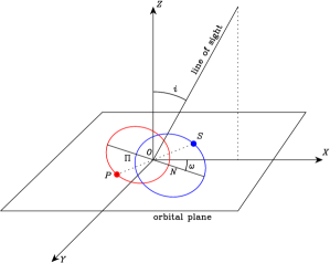
Figure 7.— Schematic for the geometry of the SMBHB system. The orbital plane is located in the $XOY$-plane, and the observer is located in the $XOZ$-plane. $\Pi$ and $N$ denote locations of the periastron. $P$ and $S$ denote locations of the primary and secondary black hole at the start of observations ($t=0$). The parameter $\omega$ denotes the angle of the periastron with respect to the $X$-axis. The parameter $\phi_{0}$ denotes the fraction of an orbit that the periastron occurs, prior to $t=0$. Thus, at $t=0$, the primary black hole is at an angle $\angle NOP$ from the periastron.

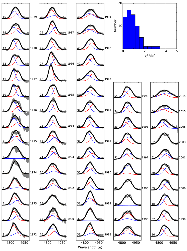
Figure 8.— Best fit of the H$\beta$ spectral profiles, which are averaged over an interval of $150$ days. Blue and red lines are components from the binary BLRs, and black line is the sum of these two components. The top right inset shows the $\chi^{2}$ distribution of the best fit.

Table 4 Parameters of the supermassive black hole binary in NGC 5548

Parameter	Physical Meaning	Value	Unit
$T_{\bullet}$	Orbital period in rest frame	$13.90\pm 0.85$	yr
$M_{\bullet}$	Total mass	$27.66\pm 8.66$	$10^{7}M_{\odot}$
$a_{\bullet}$	Semi-major axis	$21.73\pm 2.43$	light-day
$M_{\bullet,1}\sin^{3}i$	Primary mass	$0.92^{+0.19}_{-0.24}$	$10^{7}M_{\odot}$
$q$	Mass ratio	$1.00^{+0.00}_{-0.32}$	$\cdots$
$e_{\bullet}$	Eccentricity of the orbit	$0.13^{+0.18}_{-0.13}$	$\cdots$
$\phi_{0}$	Fraction of the orbit that the periastron occurs, prior to $t=0$	$0.78^{+0.05}_{-0.06}$	$\cdots$
$\omega$	Angle of the periastron with respect to X-axis	$202^{+20}_{-17}$	deg
$i$	Inclination of the orbit	$23.9\pm 3.5$	deg

Note. — The total mass of the binary is determined from the $M_{\bullet}-\sigma_{\star}$ relation of Kormendy & Ho (2013) for classical bulges. The orbital period is set by the rest-frame mean period in Table 3.

4.5. SMBHB model

Periodicity is one generic feature of SMBHB systems, not only in the orbital motion, but also in various observational properties related to the orbital motion. Numerical simulations have extensively shown that the SMBHB’s orbital motion gives rise to enhanced periodicity in the mass accretion rates onto each black holes (e.g., Hayasaki et al. 2008, 2013; Shi et al. 2012; Farris et al. 2014 and references therein). This motivates systematic searches of SMBHB candidates through periodic optical variability (e.g., Graham et al. 2015b; Liu et al. 2015b). On the other hand, the motion of the BLR gas surrounding the black holes is influenced, if not governed, by the binary, and the broad emission lines should carry the information of the binary’s orbital motion in their profiles (Eracleous et al. 2012; Shen & Loeb 2010; Popović 2012; Liu et al. 2015a). Therefore, a SMBHB can naturally, simultaneously explain all the periodicity in NGC 5548, namely, the periodicity in the 5100 Å continuum, H$\beta$ integrated fluxes, and H$\beta$ profiles. Below we will develop a simple toy SMBHB model for the H$\beta$ profiles of NGC 5548 and discuss the implications for the connection between the continuum variation and the orbital motion.

5. A Toy SMBHB Model for the H$\beta$ Profiles

With the above evidence that NGC 5548 has a SMBHB in its center, we now turn to explore the orbital information of the system. Below, we construct a simple toy model for a binary black hole pair, each having its own accretion disk and BLR, and use this model to decompose the observed profiles of the H$\beta$ line (Popovic et al. 2000; Popović 2012).

5.1. Orbital parameters

As the masses of the accretion disks and BLRs are negligible compared to those of the black holes, the orbital motion of the binary is simplified to a two-body problem. We create a Cartesian coordinate system ($X,Y,Z$) with its origin at the center of mass of the binary. The orbital plane is located in the $XOY-$plane. Figure 7 illustrates a schematic for the geometry of the SMBHB system. In Appendix D, we give a detailed derivation of equations for the orbital motion of the binary system. The binary orbit is completely described by seven parameters:

• mass of the primary black hole $M_{\bullet,1}$,

• mass ratio $q$,

• orbital eccentricity $e_{\bullet}$,

• orbital period $T_{\bullet}$ (rest-frame),

• angle $\omega$ of the periastron with respect to the $X-$axis,

• time fraction $\phi_{0}$ of the orbit (in term of the period) that the periastron occurs, prior to the start of the observations ($t=0$),

• inclination angle $i$.

The inclination angle is degenerate with $M_{\bullet,1}$ along lines of constant $M_{\bullet,1}\sin^{3}i$. We use $M_{\bullet,1}\sin^{3}i$ as a single parameter in the calculations and determine their respective values using the otherwise measured total mass of the binary (e.g., from the $M_{\bullet}-\sigma_{\star}$ relation). We also fix the orbital period by the rest-frame mean period listed in Table 3, i.e., $T_{\bullet}=14.14/(1+z)=13.90$ yr.

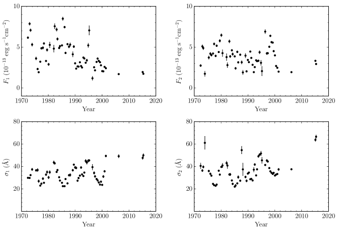
Figure 9.— The best parameters $F_{j}$ and $\sigma_{j}$ for 65 averaged H$\beta$ profiles over time (see Equation (9)).

5.2. Decomposition of H$\beta$ profiles

To smear out the stochastic, short-term changes of the profiles, we average the H$\beta$ spectra over an interval of 150 days, chosen to be similar to the characteristic timescale in the light curves of continuum and H$\beta$ fluxes (see Section 3.1). Provided that the interval is much less than the orbital period, such an averaging procedure does not influence our results. As explained in Section 2.3, we pre-select out the spectra during relatively high states of NGC 5548 ($F_{\rm AGN}/F_{\rm gal}\lower 2.0pt\hbox{$\,\buildrel\scriptstyle>\over{\scriptstyle\sim}\,$}0.7$). This leaves us with 65 averaged H$\beta$ profiles, as plotted in Figure 8.

We assume that the velocity profiles of the binary BLR components are Gaussian, with shifting velocities following the line-of-sight velocities of their associated black holes, $V_{\rm LOS,1}$ and $V_{\rm LOS,2}$. To be specific, the profiles are described by

$$f_{j}(v)=\frac{F_{j}}{\sqrt{2\pi}\sigma_{j}}\exp\left[-\frac{(v-V_{{\rm LOS},j})^{2}}{2(\sigma_{j})^{2}}\right],$$ (9)

where $v$ is velocity, $j=1,2$ correspond to the two components, and $\sigma_{j}$ and $F_{j}$ are the velocity dispersion and total flux of the profile, respectively, which are the free parameters to be determined. Note that $F_{j}$ and $\sigma_{j}$ are different with different H$\beta$ spectra (since the H$\beta$ line is time-varying), so that we have hundreds of free parameters, making a simultaneous determination of them impossible. Our decomposition procedure is as follows. Given a set of orbital parameters, we first calculate the line-of-sight velocities of the binary and then use Equation (9) to fit each averaged H$\beta$ spectrum based on $\chi^{2}$ minimization. The minimum $\chi^{2}$ of each fit is denoted by $\chi_{i,\rm min}^{2}$; there are in total 65 $\chi_{\rm min}^{2}$. We sum up these $\chi_{i,\rm min}^{2}$ as

$$\chi_{\rm tot}^{2}=\sum_{i}\chi_{i,\rm min}^{2}$$ (10)

and determine the best orbital parameters by searching for the minimum $\chi_{\rm tot}^{2}$. As an independent check, we expect that the obtained parameters $F_{j}$ and $\sigma_{j}$ should also change periodically with time.

It is computationally expensive to fit 65 averaged H$\beta$ profiles every time given a new set of orbital parameters, meaning that we cannot efficiently explore all the parameter space to find out the minimum $\chi_{\rm tot}^{2}$. Instead, we only survey over a mesh grid of the probable orbital parameters. We can impose prior constraints on the parameters from general considerations. The range of mass ratio is set to $q\sim[0.3,1.0]$, as the morphology of NGC 5548 suggests it experienced a major merger event (Section 1). The orbit eccentricity must be small, or else the binary will spend most its time around the apastron. In this case, most of the H$\beta$ profiles will not be as asymmetric as observed (see Figure 5). We accordingly set a range of eccentricity $e_{\bullet}\sim[0,0.5]$. The inclination angle should be not larger than the opening angle of the dusty torus, or else the BLRs will be obscured (e.g., Lawrence & Elvis 2010). We set the range of inclination angle $i\lower 2.0pt\hbox{$\,\buildrel\scriptstyle<\over{\scriptstyle\sim}\,$}50^{\circ}$. This yields an upper limit to $M_{\bullet,1}\sin^{3}i\lower 2.0pt\hbox{$\,\buildrel\scriptstyle<\over{\scriptstyle\sim}\,$}9\times 10^{7}M_{\odot}$. The ranges for the rest of the free parameters are $\omega\sim[0,2\pi]$ and $\phi_{0}\sim[0,1]$. After determining the best-fit orbital parameters, we estimate the associated uncertainties from the 68.3% confidence ranges (“$1\sigma$”) of the $\chi^{2}_{\rm tot}$ curves. The resulting best-fit orbital parameters are tabulated in Table 4. The binary has a large mass ratio close to 1 ($q>0.68$), consistent with the major merger scenario for the tidal morphology of the host galaxy. The orbit has an eccentricity of $e_{\bullet}<0.31$ and an inclination angle of $23.9\pm 3.5$ degrees.

In Figure 8, we show the best fits of the averaged profiles and the corresponding $\chi^{2}$-distribution. Generally, considering the simplicity of our decomposition model, most of the H$\beta$ profiles are well reproduced, except for a few with tiny lumps during some epochs (e.g., 1974-1977 and 2000-2003). These tiny lumps may arise from over-dense regions in the BLRs due to the tidal perturbations of the binary, which may induce inhomogeneities in the BLR gas distribution (e.g., Bogdanović et al. 2008). Moreover, when the line-of-sight velocities of the two components are nearly identical (both go to zero), the fitting is degenerate and only finds a solution for one component. This is why in panels 5, 6, 18, 32, 48, 49, and 62 the obtained flux of one component is zero. Figure 9 plots the best-fit parameters $F_{j}$ and $\sigma_{j}$ for the 65 H$\beta$ profiles, excluding the points whose fits are degenerate due to nearly identical line-of-sight velocities of the two components. As can be seen, it is no surprise that there appears to be some periodicity in these parameters over time, which just reflects that the H$\beta$ profiles have periodic variations, as we have demonstrated through the epoch-folding scheme. It is worth mentioning that the variability of the line dispersion of each component is due to the changes in the ionizing luminosity of the disk(s), as reflected in the 5100 Å light curve.

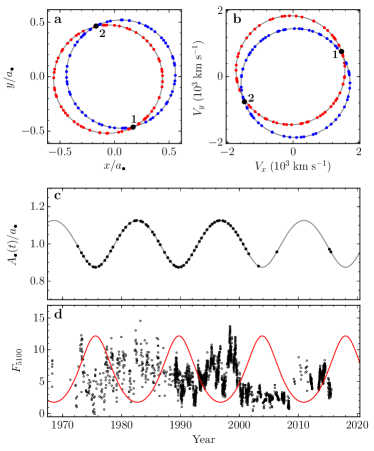
Figure 10.— The (a) orbit, (b) velocity, (c) separation between the black hole binary in the orbital plane, and (d) relation between the continuum fluxes and binary separation. Small dots in panels a-c represent the points associated with the averaged spectra as shown in Figure 8. Large black dots labelled “1” and “2” in panels a and b mark the initial positions and velocities of the binary. In panel d, for illustrative purposes, we superpose a red curve $F_{5100}=a(A_{\bullet}/a_{\bullet})^{-2}+b$, with $a=20$ and $b=-14$, to compare the 5100 Å  light curve with the orbital motion. There appears to be a time offset of a few years between the orbital motion (pericenter passage) and the continuum variations.

5.3. The continuum variations lag behind the orbital motion?

Figures 10a$-$10c show the trajectories, velocities, and separation of the SMBHB system in the orbital plane deduced from our model. To compare the 5100 Å light curve with the orbital motion, in Figure 10d we superpose a red curve to indicate the inverse square of the binary’s separation as $a(A_{\bullet}/a_{\bullet})^{-2}+b$, with $a=20$ and $b=-14$. The choice of these values is arbitrary and just for illustrative purposes. There appears to be a time offset of a few years between the orbital motion (pericenter passage) and the continuum variations.

We suspect that such a time offset may be due to the (different) retarded responses of the accretion disks to their interplay with the binary. The interplay between the disks and the binary includes: (1) perturbations in the disks induced by the tidal torques; (2) modulation of the mass accretion rates onto the disks by the orbital motion of the binary. The latter is well studied by numerical simulations (e.g., Farris et al. 2014, and references therein). At the apastron (rather than periastron) passage, the black holes are closest to the inner edge of the circumbinary disk and therefore are easiest to obtain the gas. If further taking into account the free-fall time for the gas streaming from the inner edge of the circumbinary disk to the black holes, there will be a time delay between the peak of the mass accretion rates onto the black holes and the apastron passage (e.g., Artymowicz & Lubow 1996; Hayasaki et al. 2013). Moreover, the system is now no longer stationary but highly time dependent; but the viscous accretion timescale, which reflects the timescale of an accretion disk responding to changes in mass accretion rate, is on the order of $10^{5-7}$ yr (Frank et al. 2002), much longer that the modulation timescale of mass accretion. Therefore, it is inappropriate to directly use mass accretion rate to indicate disk emission. The dynamics of accretion disks with black hole tidal interaction may have special observational properties, which deserves a dedicated investigation in the future (see the preliminary studies of Tanaka 2013 and Farris et al. 2015).

6. Discussions on the SMBHB scenario

The intensive spectroscopic and photometric data of NGC 5548 over a time span of four decades allow us to tightly constrain the possible explanations for the periodicity found in the light curves of the 5100 Å continuum and H$\beta$ flux, as well as in the variations of the H$\beta$ profile. The SMBHB scenario can naturally account for the three types of periodic variations observed in NGC 5548. However, the following points merit further thought.

Although we ascribe the periodicity in the light curves of the continuum and H$\beta$ fluxes to binary motion, we cannot specify in more detail how the (periodic) binary motion translates into periodic luminosity modulation. A general, qualitative explanation is that the binary’s orbital motion induces periodic enhancements of the mass accretion rate onto each black hole (e.g., Farris et al. 2014). As illustrated in Section 5.3, it is not as straightforward as usually thought to link the disk emission with mass accretion rate. One needs to carefully investigate the dynamics of accretion disks around binary black holes and the influences of the tidal torques (e.g., Liu & Shapiro 2010). On the other hand, recently D’Orazio et al. (2015b) interpreted the periodicity of the light curve by relativistic Doppler boosting and successfully applied their model to the periodic light curve of PG 1302-102 (Graham et al. 2015a). For NGC 5548, Doppler boosting is unimportant because the line-of-sight velocities of the binary are non-relativistic ($V/c<10^{-2}$; see Figure 10b).

We directly interpret the observed periodicity as the (redshifted) orbital period of the binary. However, recent hydrodynamic numerical simulations tracked mass accretion onto the binary and showed that there may be multiple periodic components of variability in accretion rate (e.g., Farris et al. 2014; Charisi et al. 2015; D’Orazio et al. 2015a), which may lead to periodic variations in continuum flux. In some cases, depending on the mass ratio of the binary, the dominant periodicity may not correspond to the orbital period. However, we do not yet know whether the variations of the H$\beta$ profiles have similarly multiple periodic components.

For simplicity, we use two Gaussians to delineate the H$\beta$ emission lines from the BLR around each black hole, assuming that the two BLRs are well separated and virialized. On the one hand, tidal torques from the binary induce perturbations to the BLR gas, giving rise to some inhomogeneous features, such as tidal arms or clumpy filaments (Bogdanović et al. 2008). Clearly, these features, which may be responsible for tiny lumps appearing in the H$\beta$ profiles (see Section 5.2), are time varying and closely linked to the binary orbit. On the other hand, the semi-major axis of the binary is $\sim 22$ light-days, only marginally larger than or even comparable with the BLR sizes measured from the reverberation-mapping observations (Bentz et al. 2013). The Roche lobes of the binary system have a size of (Eggleton 1983)

$$\frac{R_{\rm L}}{a_{\bullet}}=\frac{0.49q^{2/3}}{0.6q^{2/3}+\ln(1+q^{1/3})}\sim 0.4,$$ (11)

for a circular orbit ($e_{\bullet}=0$) with equal mass ($q=1$). The size of the BLR associated with each black hole can be estimated from the $R_{\rm BLR}-L$ relation of Bentz et al. (2013) as

$$R_{\rm BLR}=33.6\left(\frac{L_{\rm 5100}}{10^{44}~{}{\rm erg~{}s^{-1}}}\right)^{0.533}\sim 10~{}\text{light-days},$$ (12)

where we assume that the black holes in the pair have the same luminosity and adopt the typical mean value $L_{\rm 5100}=10^{43}~{}{\rm erg~{}s^{-1}}$ using a luminosity distance of 75 Mpc. Considering that the 5100 Å luminosity varies by a large factor of more than 6 (see Figure 3), the above estimates indicate that the two BLRs are plausibly in contact during the intermediate or high states of NGC 5548 (in which $R_{\rm BLR}>R_{\rm L}$). In such cases, there probably will be a circumbinary BLR component. Meanwhile, a portion of the two BLRs may be illuminated by ionizing photons from both black holes (Shen & Loeb 2010). Therefore, a Gaussian is only a very simplified approximation to the realistic H$\beta$ profiles and the obtained orbital parameters (such as the mass ratio, eccentricity, and inclination, etc.) should be taken with caution. These values are meant to demonstrate the capability of reproducing the H$\beta$ profiles with a SMBHB model. More sophisticated SMBHB models are required to account for the above mentioned effects.

Finally, we present an outlook for subsequent works and future observations to further reinforce the presence of a SMBHB system in NGC 5548, with the following remarks.

1. If each black hole produces radio emission, the future Event Horizon Telescope, with an angular resolution of $\sim 20\,\mu$as (Fish et al. 2013), will be capable of spatially resolving the radio core of NGC 5548 (Ho & Ulvestad 2001) into two components separated by $\sim 22$ light-days ($\sim 50\,\mu$as). This will provide direct evidence for the SMBHB.

2. We only apply our SMBHB model to decompose the averaged H$\beta$ profiles so as to smear out the short-term stochastic changes in the profiles. It would be interesting to study in detail how the H$\beta$ profile varies on short timescale of hundreds of days (e.g., Flohic & Eracleous 2008). As demonstrated by Shen & Loeb (2010) using a heuristic toy model, the reverberation behavior of the broad emission lines from a binary system should be distinguishable from that from a single black hole, considering that the BLR geometry is different and there are two ionizing sources in binaries. Such studies will also shed light on the BLR dynamics surrounding a SMBHB.

3. From the extensive database for NGC 5548, we can also use other prominent emission lines (such as H$\alpha$) to study their profile variations by applying the same procedure as in this work and test if there exists similar periodicity.

4. We can use $N$-body simulations to recover the merger history of NGC 5548 by trying to reproduce in detail its observed morphology. This will help to better understand the dynamical evolution of the SMBHB (e.g., Begelman et al. 1980).

5. Continued monitoring of NGC 5548 will track more cycles of the binary orbit and improve the measurement uncertainties of the periods.

7. Conclusions

We propose that a SMBHB plausibly resides in the galactic center of NGC 5548 based on four decades of spectroscopic data. The two peaks of the H$\beta$ profiles shift and merge in a systematic manner with a period of $\sim 14$ yr, which agrees with the period observed in the long-term variations in both the continuum and H$\beta$ fluxes (see Figures 3 and 5). In addition, the morphology of NGC 5548 shows two long tidal tails (see Figure 1 and Tyson et al. 1998), indicative of a major merger event that occurred $\sim 1$ Gyr ago. These lines of observations make NGC 5548 one of the nearest and best sub-parsec SMBHB candidates known to date. The SMBHB has a total mass of $2.8\times 10^{8}M_{\odot}$ from the $M_{\bullet}-\sigma_{\star}$ relation and a semi-major axis of 21.73 light-days from Kepler’s third law, indicating that the SMBHB has an extremely sub-parsec separation. Using our toy SMBHB model, we demonstrate that the complex, secularly varying H$\beta$ profiles can be reproduced by orbital motion of the SMBHB with a large mass ratio ($q>0.68$) and an eccentricity of $e_{\bullet}<0.31$, viewed at an inclination angle of 23.9 degrees (see Table 4).

The SMBHB will coalesce within $\sim 6\times 10^{6}a_{-2}^{4}m_{8}^{-3}q^{-1}(1+q)^{2}$ yr and radiate gravitational waves at a frequency of $2/T_{\bullet}\sim 7\times 10^{-9}m_{8}^{1/2}a_{-2}^{-3/2}$ Hz, where $a_{-2}=a_{\bullet}/10^{-2}$ pc. The expected strain amplitude of the intrinsic gravitation wave is $h_{s}\approx 9\times 10^{-17}m_{8}^{2}a_{-2}^{-1}q(1+q)^{-2}d_{75}^{-1}$ (e.g., see Graham et al. 2015b), where $d_{75}=d_{\rm L}/75\,{\rm Mpc}$ is the distance to the observer. The proximity of NGC 5548 makes its SMBHB system an excellent target for detection of gravitational waves through the Pulsar Timing Array (e.g., Moore et al. 2015; Sessana 2015).

In this Appendix, we present detailed information on the published data used in our analysis, a study on the host galaxy contamination on H$\beta$ profiles, a test of the influences of the varying H$\beta$ line width (due to the periodic variations in the 5100 Å continuum) on the epoch-folding results, and a derivation of the SMBHB orbital motion used in our model for the H$\beta$ profiles.

Appendix A A. Historical observations

Figure 11.— A total of 924 H$\beta$ profiles of NGC 5548 from 1972 to 2015.

A.1. A.1. Data sources

We compiled the spectroscopic and photometric data for NGC 5548 from the literature in Tables 1 and 1. In addition, as described Section 2.1, we made new observations of our own in 2015. The majority of the data are publicly available. The others are kindly provided by the corresponding authors of the listed references. The archival data of the 5100 Å continuum fluxes and the H$\beta$ profiles from 1972 to 2001 compiled in [105] were provided by S. G. Sergeev. The spectra from 1995 presented in [53] were provided by T. Iijima, and those from 1998–2004 presented in [97] were provided by L. Č. Popović. The mean spectra from 2008 presented in [21] was provided by K. Denney. Figure 11 shows a total of 924 H$\beta$ profiles taken over four decades.

A.2. A.2. Flux conversion

Some studies only presented continuum measurements in the $V$ band or at 1350 Å. To convert these data into continuum flux densities at 5100 Å, we use the following relations:

• The $V$-band flux density, $F_{\lambda}(V)$, can be converted to 5100 Å flux density through

  $$F_{5100}=(0.946\pm 0.072)F_{\lambda}(V),$$ (A1)

  as determined from simultaneous observations (Romanishin et al. 102).

• For photometric observations in the $V$ band, we first convert the magnitudes into flux densities by adopting the zero point $F_{\lambda}(V=0)=3.92\times 10^{-9}\,{\rm erg~{}s^{-1}~{}cm^{-2}}\textrm{\AA}^{-1}$ (Johnson 55) and then apply relation (A1).

• The flux density at 1350 Å can be converted to 5100 Å through the relation

  $$\log\left(\frac{L_{5100}}{10^{43}~{}{\rm erg~{}s^{-1}}}\right)=(0.55\pm 0.05)+(0.63\pm 0.12)\log\left(\frac{L_{1350}}{10^{44}~{}{\rm erg~{}s^{-1}}}\right),$$ (A2)

  which was derived from simultaneous observations in the UV and optical bands (Kilerci Eser et al. 58). Note that this relation is based on a luminosity distance of $72.5\pm 7.0$ Mpc for NGC 5548.

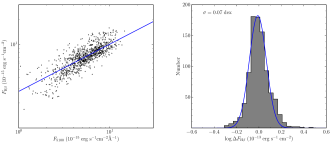
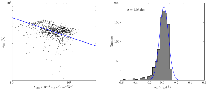
Figure 12.— Left: relations between the 5100 Å continuum flux and (top) the H$\beta$ line flux and (bottom) the H$\beta$ line dispersion. The narrow H$\beta$ component is subtracted and the H$\beta$ flux is calculated over a wavelength window 4719-5001 Å in the rest frame. Solid line represents the best fit to the data. Right: residuals of (top) the H$\beta$ line flux and (bottom) the H$\beta$ line dispersion using the corresponding best-fit relation. Solid line represents a fit to the residuals by a Gaussian function.

Appendix B B. Host contamination of the H$\beta$ profile

In this section, we test whether contamination from host galaxy starlight causes the double-peaked profile of H$\beta$ that appears in most of the observations. Following [4], we adopt an 11 Gyr, solar metallicity, single-burst spectrum from [13] to model the host galaxy starlight. This template is convolved with a Gaussian with a standard deviation of $\sim 15$ Å to account for the spectral resolution of the data. We assume that the optical continuum of the AGN can be described by a power law, and that the broad H$\beta$ profile is a single Gaussian. The H$\beta$ flux is related to the continuum according to the following relation, which is empirically determined from the data compiled in this work:

$$\log\left(\frac{F_{{\rm H}\beta}}{10^{-13}\,\rm erg~{}s^{-1}~{}cm^{-2}}\right)=0.44+0.57\log\left(\frac{F_{5100}}{10^{-15}\,\rm erg~{}s^{-1}~{}cm^{-2}~{}{\text{\AA}}^{-1}}\right).$$ (B1)

The obtained coefficients are generally consistent with [105]’s results. The dispersion of the Gaussian for H$\beta$ depends on the continuum as

$$\log\left(\frac{\sigma_{{}_{\rm H\beta}}}{\text{\AA}}\right)=1.81-0.25\log\left(\frac{F_{5100}}{10^{-15}\,\rm erg~{}s^{-1}~{}cm^{-2}~{}{\text{\AA}}^{-1}}\right),$$ (B2)

again based on the data used in this work. The scatter of the latter fit is about 0.06 dex, which we will use in next section. In Figure 12, we show the relations between the 5100 Å continuum flux and the H$\beta$ line flux and the H$\beta$ line dispersion. For simplicity, the power-law index is fixed to $-$0.25, as expected from simple photoionization theory. We generate a mock spectrum by adding up the three components, namely the host starlight, the AGN continuum, and the H$\beta$ line. Since we only focus on the effect of host galaxy contamination on the broad H$\beta$ profile, we neglect other components such as narrow H$\beta$, [O III], Balmer continuum, and Fe II  blends.

We set the host galaxy flux at 5100 Å to the value determined from the AGN Watch campaigns, $F_{\rm gal}=3.75\times 10^{-15}\,\rm erg~{}s^{-1}~{}cm^{-2}~{}{\text{\AA}}^{-1}$ (Peterson et al. 89). Note that this choice does not affect our test because the results only depend on the flux ratio between the central AGN and the host galaxy starlight $F_{\rm AGN}/F_{\rm gal}$ at 5100 Å. We then use the standard procedure from [105], as described in Section 2.3, to remove the continuum of the mock spectrum and isolate the broad H$\beta$ line. The top panel of Figure 13 shows the resulting broad H$\beta$ profiles for different values of $F_{\rm AGN}/F_{\rm gal}$. As can be seen, the broad H$\beta$ profile is significantly contaminated by host galaxy light when $F_{\rm AGN}/F_{\rm gal}\lower 2.0pt\hbox{$\,\buildrel\scriptstyle<\over{\scriptstyle\sim}\,$}0.5$. We also calculate the integrated H$\beta$ flux over a wavelength window $4714-4933$ Å (rest-frame) and show its dependence on $F_{\rm AGN}/F_{\rm gal}$ in the bottom panel of Figure 13. The changes in the H$\beta$ fluxes are less than 10% for $F_{\rm AGN}/F_{\rm gal}\lower 2.0pt\hbox{$\,\buildrel\scriptstyle>\over{\scriptstyle\sim}\,$}0.2$.

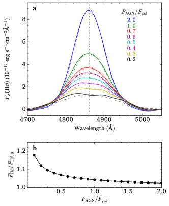
Figure 13.— The effect of host galaxy contamination on (a) the profile of H$\beta$ and (b) H$\beta$ flux for different ratios between the AGN flux and the host galaxy starlight ($F_{\rm AGN}/F_{\rm gal}$) at 5100 Å. The host galaxy starlight is set to a typical value of $F_{\rm gal}=3.75\times 10^{-15}~{}\rm erg~{}s^{-1}~{}cm^{-2}~{}\text{\AA}^{-1}$. In the top panel, solid lines represent the obtained H$\beta$ profiles from the mock spectra and dashed lines the input H$\beta$ profiles (see the text for details). Vertical line shows the wavelength center of H$\beta$ line. In the bottom panel, vertical axis is the ratio between the obtained ($F_{\rm H\beta}$) and input integrated H$\beta$ fluxes ($F_{\rm H\beta,0}$) .

Appendix C C. Influences of the Periodic 5100 Å Variations on the Epoch-folding of the Broad H$\beta$ Profiles

We note that simply from the relation between BLR sizes and AGN 5100 Å luminosity and the virial relation (e.g., Peterson et al. 90, Bentz et al. 6, Simic & Popovic 111), the H$\beta$ line width is closely correlated to the 5100 Å luminosity. As a result, the periodic continuum variations of NGC 5548 certainly lead to periodic changes in H$\beta$ line width. To see how the line width of H$\beta$ profile (in terms of the line dispersion) influences the epoch-folding results, we simulate mock H$\beta$ profiles using a single Gaussian, as follows.

• Set the center of the Gaussian to be 4861 Å (in the rest frame).

• Set the dispersion $\sigma_{\rm H\beta}$ using Equation (B2), with a scatter of 0.06 dex.

• Set the noise of the Gaussian at each wavelength bin by the standard deviation of the observation data over all the epochs at the same wavelength bin.

Figure 14a shows the epoch-folding results for the mock data. Compared with the epoch-folding results for the real data in Figure 5, the simulated profiles show a similar periodicity of $\sim$14 yr, directly owing to the periodicity in the light curve of 5100 Å continuum.

However, for the simulation data, we can just make a simple transformation for the H$\beta$ profiles to eliminate the influences of the varying line dispersion,

$$\frac{\lambda-\lambda_{0}}{\sigma_{\rm old}}\rightarrow\frac{\lambda-\lambda_{0}}{\sigma_{\rm new}},$$ (C1)

where $\lambda_{0}$ is the wavelength center of H$\beta$ profiles and $\sigma_{\rm old}$ and $\sigma_{\rm new}$ are the original and new line dispersion, respectively. We transform all the simulated H$\beta$ profiles to $\sigma_{\rm new}=50~{}\text{\AA}$. Similarly, we can also perform the same transformation for the observation data. Figures 14b and 14c show the comparison of the epoch-folding results by including the transformation. As expected, the periodicity disappears for the simulated data but is still present in the observation data, indicating that the observed periodicity is not entirely an artifact of the periodicity in the 5100 Å continuum.

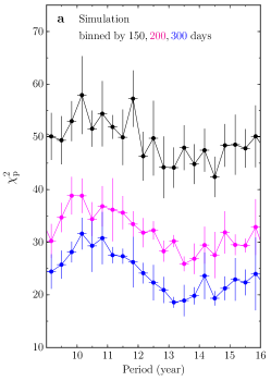
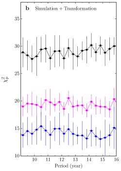
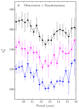
Figure 14.— Same as Figure 5 but for (a) simulation data, (b) simulation data with a transformation, and (c) observation data with a transformation (see the text for details).

Appendix D D. SMBHB orbital motion

Figure 7 illustrates a schematic for the geometry of the SMBHB system. The observer is in the $XOZ$-plane, and the orbital plane is defined to be the $XOY$-plane, viewed at an inclination angle $i$. Given the total mass of the binary system $M_{\bullet}$, the orbital period $T_{\bullet}$ (rest-frame) and the orbital semi-major axis $a_{\bullet}$ are related by

$$a_{\bullet}=\left(\frac{GM_{\bullet}T_{\bullet}^{2}}{4\pi^{2}}\right)^{1/3}.$$ (D1)

The separation between the binary black holes is

$$A_{\bullet}=\frac{a_{\bullet}(1-e_{\bullet}^{2})}{1+e_{\bullet}\cos\theta},$$ (D2)

where $e_{\bullet}$ is the orbital eccentricity and $\theta$ is the angle from periastron, depending on the time as

$$\frac{d\theta}{dt}=\frac{2\pi}{T_{\bullet}}\frac{\left[1+e_{\bullet}\cos\theta(t+t_{0})\right]^{2}}{(1+e_{\bullet}^{2})^{3/2}},$$ (D3)

where $t_{0}=\phi_{0}T_{\bullet}$ is the time prior to the start of data-taking that the binary is at periastron. By introducing the eccentric anomaly $\xi$,

$$\sin\theta=\frac{\cos\xi-e_{\bullet}}{1-e_{\bullet}\cos\xi},$$ (D4)

we obtain a simple equation for $\xi$ (46, p.38)

$$\xi-e_{\bullet}\sin\xi=\frac{2\pi}{T_{\bullet}}(t+t_{0}).$$ (D5)

For an orbit with the periastron at an angle $\omega$ from the $X$-axis, the positions of the primary and the secondary black holes are

$$(x_{1},y_{1})=-\frac{qA_{\bullet}}{1+q}\left[\cos(\theta+\omega),\sin(\theta+\omega)\right],$$ (D6)

and

$$(x_{2},y_{2})=\frac{A_{\bullet}}{1+q}\left[\cos(\theta+\omega),\sin(\theta+\omega)\right],$$ (D7)

respectively, where $q$ is the mass ratio of the binary. Their corresponding velocities are

$$(v_{x,1},v_{y,1})=-\frac{q}{1+q}\left[v_{r}\cos(\theta+\omega)-v_{\theta}\sin(\theta+\omega),v_{r}\sin(\theta+\omega)+v_{\theta}\cos(\theta+\omega)\right],$$ (D8)

and

$$(v_{x,2},v_{y,2})=\frac{1}{1+q}\left[v_{r}\cos(\theta+\omega)-v_{\theta}\sin(\theta+\omega),v_{r}\sin(\theta+\omega)+v_{\theta}\cos(\theta+\omega)\right],$$ (D9)

where $v_{r}$ and $v_{\theta}$ are given by

$$v_{r}=\frac{dA_{\bullet}}{dt},~{}~{}~{}~{}~{}~{}v_{\theta}=A_{\bullet}\frac{d\theta}{dt}.$$ (D10)

The line-of-sight velocities of the binary are $V_{\rm LOS,1}=v_{x,1}\sin i$ and $V_{\rm LOS,2}=v_{x,2}\sin i$, respectively.

References

- Arav et al. [2014] Arav, N., Chamberlain, C., Kriss, G. A., et al. 2015, A&A, 577, 37
- Artymowicz & Lubow [1996] Artymowicz, P., & Lubow, S. H. 1996, ApJ, 467, L77
- Bardeen & Petterson [1975] Bardeen, J. M., & Petterson, J. A. 1975, ApJ, 195, L65
- Barth et al. [2013] Barth, A. J., Pancoast, A., Bennert, V. N., et al. 2013, ApJ, 769, 128
- Begelman et al. [1980] Begelman, M. C., Blandford, R. D., & Rees, M. J. 1980, Nature, 287, 307
- Bentz et al. [2013] Bentz, M. C., Denney, K. D., Grier, C. J., et al. 2013, ApJ, 767, 149
- Betnz et al. [2007] Bentz, M. C., Denney, K. D., Cackett, E. M., et al. 2007, ApJ, 662, 205
- Bentz et al. [2009] Bentz, M. C., Walsh, J. L., Barth, A. J., et al. 2009, ApJ, 705, 199
- Bogdanović et al. [2008] Bogdanović, T., Smith, B. D., Sigurdsson, S., & Eracleous, M. 2008, ApJS, 174, 455
- Bon et al. [2012] Bon, E., Jovanović, P., Marziani, P., et al. 2012, ApJ, 759, 118
- Boroson & Lauer [2009] Boroson, T. A., & Lauer, T. R. 2009, Nature, 458, 53
- Bottorff et al. [2002] Bottorff, M. C., Baldwin, J. A., Ferland, G. J., Ferguson, J. W., & Korista, K. T. 2002, ApJ, 581, 932
- Bruzual & Charlot [2003] Bruzual, G., & Charlot, S. 2003, MNRAS, 344, 1000
- Chakrabarti & Wiita [1993] Chakrabarti, S. K., & Wiita, P. J. 1993, ApJ, 411, 602
- Charisi et al. [2015] Charisi, M., Bartos, I., Haiman, Z., Price-Whelan, A. M., & Márka, S. 2015, MNRAS, 454, L21
- Chen et al. [1989] Chen, K., Halpern, J. P., & Filippenko, A. V. 1989, ApJ, 339, 742
- Chiang & Blaes [2003] Chiang, J., & Blaes, O. 2003, ApJ, 586, 97
- Comerford et al. [2015] Comerford, J. M., Pooley, D., Barrows, R. S., et al. 2015, ApJ, 806, 219
- De Rosa et al. [2015] De Rosa, G., Peterson, B. M., Ely, J., et al. 2015, ApJ, 806, 128
- Denney et al. [2009] Denney, K. D., Peterson, B. M., Dietrich, M., Vestergaard, M., & Bentz, M. C. 2009, ApJ, 692, 246
- Denney et al. [2010] Denney, K., Peterson, B. M., Pogge, R. W., et al. 2010, ApJ, 721, 715
- D’Orazio et al. [2015a] D’Orazio, D. J., Haiman, Z., Duffell, P., Farris, B. D., & MacFadyen, A. I. 2015a, MNRAS, 452, 2540
- D’Orazio et al. [2015b] D’Orazio, D. J., Haiman, Z., & Schiminovich, D. 2015b, Nature, 525, 351
- Du et al. [2014] Du, P., Hu, C., Lu, K.-X., et al. 2014, ApJ, 782, 45
- Ebisuzaki et al. [1991] Ebisuzaki, T., Makino, J., & Okumura, S. K. 1991, Nature, 354, 212
- Edelson et al. [2015] Edelson, R., Gelbord, J. M., Horne, K., et al. 2015, ApJ, 806, 129
- Eggleton [1983] Eggleton, P. P. 1983, ApJ, 268, 368
- Eracleous et al. [2012] Eracleous, M., Boroson, T. A., Halpern, J. P., & Liu, J. 2012, ApJS, 201, 23
- Eracleous et al. [1997] Eracleous, M., Halpern, J. P., M. Gilbert, A., Newman, J. A., & Filippenko, A. V. 1997, ApJ, 490, 216
- Eracleous et al. [1995] Eracleous, M., Livio, M., Halpern, J. P., & Storchi-Bergmann, T. 1995, ApJ, 438, 610
- Farris et al. [2014] Farris, B. D., Duffell, P., MacFadyen, A. I., & Haiman, Z. 2014, ApJ, 783, 134
- Farris et al. [2015] Farris, B. D., Duffell, P., MacFadyen, A. I., & Haiman, Z. 2015, MNRAS, 446, L36
- Fausnaugh et al. [2015] Fausnaugh, M. M., Denney, K. D., Barth, A. J., et al. 2015, ApJ submitted (arXiv:1510.05648)
- Fish et al. [2013] Fish, V., Alef, W., & Anderson, J., et al. 2013, arXiv:1309.3519
- Flohic & Eracleous [2008] Flohic, H. M. L. G., & Eracleous, M. 2008, ApJ, 686, 138
- Frank et al. [2002] Frank, J., King, A., & Raine, A. 2002, Accretion Power in Astrophysics (Cambridge: Cambridge Univ. Press), p.98
- Fu et al. [2015] Fu, H., Myers, A. D., Djorgovski, S. G., et al. 2015, ApJ, 799, 72
- Gaskell [1983] Gaskell, C. M. 1983, Liege Int. Astophys. Colloq., 24, 473
- Gaskell & Peterson [1987] Gaskell, C. M., & Peterson, B. M. 1987, ApJS, 65, 1
- Graham et al. [2015a] Graham, M. J., Djorgovski, S. G., Stern, J., et al. 2015a, Nature, 518, 74
- Graham et al. [2015b] Graham, M. J., Djorgovski, S. G., Stern, D., et al. 2015b, MNRAS, 453, 1562
- Guo et al. [2006] Guo, D., Tao, J., & Qian, B. 2006, PASJ, 58, 503
- Hameury et al. [2009] Hameury, J.-M., Viallet, M., & Lasota, J.-P. 2009, A&A, 496, 413
- Hayasaki et al. [2008] Hayasaki, K., Mineshige, S., & Ho, L. C. 2008, ApJ, 682, 1134
- Hayasaki et al. [2013] Hayasaki, K., Saito, H., & Mineshige, S. 2013, PASJ, 65, 86
- Hilditch [2001] Hilditch, R. W. 2001, An Introduction to Close Binary Stars (Cambridge: Cambridge Univ. Press)
- Ho & Kim [2014] Ho, L. C., & Kim, M. 2014, ApJ, 789, 17
- Ho & Kim [2015] Ho, L. C., & Kim, M. 2015, ApJ, 809, 123
- Ho & Ulvestad [2001] Ho, L. C., & Ulvestad, J. S. 2001, ApJS, 133, 77
- Ho et al. [2000] Ho, L. C., Rudnick, G., Rix, H. W., et al. 2000, ApJ, 541, 120
- Ho [2008] Ho, L. C. 2008, ARA&A, 46, 475
- Ho & Peng [2001] Ho, L. C., & Peng, C. Y., 2001, ApJ, 555, 650
- Iijima & Rafanelli [1995] Iijima, T., & Rafanelli, P. 1995, A&AS, 113, 493
- Janiuk & Czerny [2011] Janiuk, A., & Czerny, B. 2011, MNRAS, 414, 2186
- Johnson [1996] Johnson, H. L. 1966, ARA&A, 4, 193
- Jovanović et al. [2010] Jovanović, P., Popović, L. Č., Stalevski, M., & Shapovalova, A. I. 2010, ApJ, 718, 168
- Kelly et al. [2009] Kelly, B. C., Bechtold, J., & Siemiginowska, A. 2009, ApJ, 698, 895
- Kilerci Eser et al. [2015] Kilerci Eser, E., Vestergaard, M., Peterson, B. M., Denney, K. D., & Bentz, M. C. 2015, ApJ, 801, 8
- King et al. [2008] King, A. R., Pringle, J. E., & Hofmann, J. A. 2008, MNRAS, 385, 1621
- Komossa et al. [2003] Komossa, S., Burwitz, V., Hasinger, G., et al. 2003, ApJ, 582, L15
- Kormendy & Ho [2013] Kormendy, J., & Ho, L. C. 2013, ARA&A, 51, 511
- Kormendy et al. [2009] Kormendy, J., Fisher, D. B., Cornell, M. E., & Bender, R. 2009, ApJS, 182, 216
- Koshida et al. [2014] Koshida, S., Minezaki, T., Yoshii, Y., et al. 2014, ApJ, 788, 159
- Larson [1996] Larsson, S. 1996, A&AS, 117, 197
- Laughlin & Korchagin [1996] Laughlin, G., & Korchagin, V., 1996, ApJ, 460, 855
- Lawrence & Elvis [2010] Lawrence, A., & Elvis, M. 2010, ApJ, 714, 561
- Lewis et al. [2010] Lewis, K. T., Eracleous, M., & StorchiBergmann, T. 2010, ApJS, 187, 416
- Li et al. [2013a] Li, Y.-R., Wang, J.-M., Cheng, C., & Qiu, J. 2013a, ApJ, 764, 16
- Li et al. [2015] Li, Y.-R., Wang, J.-M., Cheng, C., & Qiu, J. 2015, ApJ, 804, 45
- Li et al. [2013b] Li, Y.-R., Wang, J.-M., Ho, L. C., Du, P., & Bai, J.-M. 2013b, ApJ, 779, 110
- Li et al. [2014] Li, Y.-R., Wang, J.-M., Hu, C., Du, P., & Bai, J.-M. 2014, ApJ, 786, L6
- Liu et al. [2015a] Liu, J., Eracleous, M., & Halpern, J. P. 2015a, ApJ in press (arXiv:1512.01825)
- Liu et al. [2015b] Liu, T., Gezari, S., Heinis, S., et al. 2015b, ApJ, 803, L16
- Liu et al. [2014] Liu, X., Shen, Y., Bian, F., Loeb, A., & Tremaine, S. 2014, ApJ, 789, 140
- Liu & Shapiro [2010] Liu, Y. T., & Shapiro, S. L. 2010, Phys. Rev. D, 82, 123011
- Lu & Zhou [2005] Lu, J.-F., & Zhou, B.-Y. 2005, ApJ, 635, L17
- Lu et al. [2016] Lu, K.-X., Du, P., Hu, C., et al. 2016, ApJ submitted
- Lyutyi & Doroshenko [1993] Lyutyi, V. M., & Doroshenko, V. T. 1993, Astronomy Letters, 19, 405
- MacKenty [1990] MacKenty, J. W. 1990, ApJS, 72, 231
- Martin et al. [2007] Martin, R. G., Pringle, J. E., & Tout, C. A. 2007, MNRAS, 381, 1617
- Mehdipour et al. [2015] Mehdipour, M., Kaastra, J. S., Kriss, G. A., et al. 2015, A&A, 575, 22
- Merritt & Milosavljević [2005] Merritt, D., & Milosavljević, M. 2005, Living Review on Relativity, 8, 8
- Mineshige& Shields [1990] Mineshige, S., & Shields, G. A. 1990,ApJ, 351, 47
- Moore et al. [2015] Moore, C. J., Cole, R. H., & Berry, C. P. L. 2015, Classical and Quantum Gravity, 32, 015014
- Newman et al. [1997] Newman, J. A., Eracleous, M., Filippenko, A. V., & Halpern, J. P. 1997, ApJ, 485, 570
- Pacholczyk et al. [1983] Pacholczyk, A. G., Penning, W. R., Ferguson, D. H., Lubart, N. D., & Turnshek, D. 1983, Astrophys. Lett., 23, 225
- Peterson [1987] Peterson, B. M. 1987, ApJ, 312, 79
- Peterson et al. [2002] Peterson, B. M., Berlind, P., Bertram, R., et al. 2002, ApJ, 581, 197
- Peterson et al. [2013] Peterson, B. M., Denney, K. D., De Rosa, G., et al. 2013, ApJ, 779, 109
- Peterson et al. [2004] Peterson, B. M., Ferrarese, L., Gilbert, K. M., et al. 2004, ApJ, 613, 682
- Peterson et al. [1987] Peterson, B. M., Korista, K. T., & Cota, S. A. 1987, ApJ, 312, L1
- Peterson et al. [1995] Peterson, B. M., Pogge, R. W., Wanders, I., Smith, S. M., & Romanishin, W. 1995, PASP, 107, 579
- Peterson & Wandel [1999] Peterson, B. M., & Wandel, A. 1999, ApJ, 521, L95
- Peterson et al. [1998] Peterson, B. M., Wanders, I., Horne, K., et al. 1998, PASP, 110, 660
- Popović [2012] Popović, L. Č. 2012, New Astron. Rev., 56, 74
- Popovic et al. [2000] Popovic, L. Č., Mediavilla, E. G., & Pavlovic, R. 2000, Serbian Astronomical Journal, 162, 1
- Popović et al. [2008] Popović, L. Č., Shapovalova, A. I., Chavushyan, V. H., et al. 2008, PASJ, 60, 1
- Press et al. [1992] Press, W. H., Teukolsky, S. A., Vetterling, W. T., & Flannery, B. P. 1992, Numerical Recipes in FORTRAN (2nd ed.; Cambridge: Cambridge Univ. Press)
- Pringle [1996] Pringle, J. E. 1996, MNRAS, 281, 357
- Rafikov [2013] Rafikov, R. R. 2013, ApJ, 774, 144
- Roberts & Rumstay [2012] Roberts, C. A., & Rumstay, K. R. 2012, Journal of the Southeastern Association for Research in Astronomy, 6, 47
- Romanishin et al. [1995] Romanishin, W., Balonek, T. J., Ciardullo, R., et al. 1995, ApJ, 455, 516
- Rosenblatt & Malkan [1990] Rosenblatt, E. I., & Malkan, M. A. 1990, ApJ, 350, 132
- Schweizer & Seitzer [1988] Schweizer, F., & Seitzer, P. 1988, ApJ, 328, 88
- Sergeev et al. [2007] Sergeev, S. G., Doroshenko, V. T., Dzyuba, S. A., et al. 2007, ApJ, 668, 708
- Sessana [2015] Sesana, A. 2015, Astrophysics and Space Science Proceedings, 40, 147
- Shapovalova et al. [2004] Shapovalova, A. I., Doroshenko, V. T., Bochkarev, N. G., et al. 2004, A&A, 422, 925
- Shen et al. [2013] Shen, Y., Liu, X., Loeb, A., & Tremaine, S. 2013, ApJ, 775, 49
- Shen & Loeb [2010] Shen, Y., & Loeb, A. 2010, ApJ, 725, 249
- Shi et al. [2012] Shi, J.-M., Krolik, J. H., Lubow, S. H., & Hawley, J. F. 2012, ApJ, 749, 118
- Simic & Popovic [2016] Simic, S., & Popovic, L. C. 2016, Ap&SS, 361, 59
- Springel et al. [2005] Springel, V., White, S. D. M., Jenkins, A., et al. 2005, Nature, 435, 629
- Stirpe et al. [1988] Stirpe, G. M., de Bruyn, A. G., & van Groningen, E. 1988, A&A, 200, 9
- Strochi-Bergmann et al. [1997] StorchiBergmann, T., Eracleous, M., Teresa Ruiz, M., et al. 1997, ApJ, 489, 87
- Storchi-Bergmann et al. [2003] StorchiBergmann, T., Nemmen da Silva, R., Eracleous, M., et al. 2003, ApJ, 598, 956
- Strateva et al. [2003] Strateva, I. V., Strauss, M. A., Hao, L., et al. 2003, AJ, 126, 1720
- Sundelius et al. [1997] Sundelius, B., Wahde, M., Lehto, H. J., & Valtonen, M. J. 1997, ApJ, 484, 180
- Tanaka [2013] Tanaka, T. L. 2013, MNRAS, 434, 2275
- Tremaine & Davis [2014] Tremaine, S., & Davis, S. W. 2014, MNRAS, 441, 1408
- Tyson et al. [1998] Tyson, J. A., Fischer, P., Guhathakurta, P., et al. 1998, AJ, 116, 102
- Ulubay-Siddiki et al. [2009] Ulubay-Siddiki, A., Gerhard, O., & Arnaboldi, M. 2009, MNRAS, 398, 535
- Valtonen et al. [2008] Valtonen, M. J., Lehto, H. J., Nilsson, K., et al. 2008, Nature, 452, 851
- van Groningen & Wanders [1992] van Groningen, E., & Wanders, I. 1992, PASP, 104, 700
- Vestergaard & Peterson [2005] Vestergaard, M., & Peterson, B. M. 2005, ApJ, 625, 688
- Volonter et al. [2003] Volonteri, M., Haardt, F. & Madau, P., 2003, ApJ, 582, 559
- Wamsteker et al. [1990] Wamsteker, W., Rodriguez-Pascual, P., Wills, B. J., et al. 1990, ApJ, 354, 446
- Weinberg [1972] Weinberg, S. 1972, Gravitation and Cosmology (New York: Wiley), p.197
- Woo et al. [2010] Woo, J. H., Treu, T., Barth, A. J., et al. 2010, ApJ, 716, 269
- Yan et al. [2015] Yan, C.-S., Lu, Y., Dai, X., & Yu, Q. 2015, ApJ, 809, 117
- Zheng et al. [2015] Zheng, Z.-Y., Butler, N. R., Shen, Y., et al. 2015, ApJ submitted (arXiv:1512.08730)