On Characterization of Inverse Data in the Boundary Control Method

Abstract

We deal with a dynamical system

$$u_{tt}-\Delta u+qu=0 {\rm in}\,\,\,\Omega\times(0,T)$$

$$u\big{|}_{t=0}=u_{t}\big{|}_{t=0}=0 {\rm in}\,\,\,\overline{\Omega}$$

$$\partial_{\nu}u=f {\rm in}\,\,\,\partial\Omega\times[0,T]\,,$$

where $\Omega\subset{\mathbb{R}}^{n}$ is a bounded domain, $q\in L_{\infty}(\Omega)$ a real-valued function, $\nu$ the outward normal to $\partial\Omega$, $u=u^{f}(x,t)$ a solution. The input/output correspondence is realized by a response operator $R^{T}:f\mapsto u^{f}\big{|}_{\partial\Omega\times[0,T]}$ and its relevant extension by hyperbolicity $R^{2T}$. Operator $R^{2T}$ is determined by $q\big{|}_{\Omega^{T}}$, where $\Omega^{T}:=\{x\in\Omega\,|\,\,{\rm dist\,}(x,\partial\Omega)<T\}$. The inverse problem is: Given $R^{2T}$ to recover $q$ in $\Omega^{T}$. We solve this problem by the boundary control method and describe the necessary and sufficient conditions on $R^{2T}$, which provide its solvability.

1 Introduction

Motivation

The problem, which the paper is devoted to, was solved about 20 years ago by the BC-method, which is an approach to inverse problems (IPs) based on their relations to control and system theory [5, 1, 3]. However, in IP-community, there are a few versions of what ’to solve an inverse problem’ means. The versions may be ordered by levels as follows:

$1.$   to establish injectivity of the correspondence ‘parameters under reconstruction $\to$ inverse data’, what allows one to claim that the data determine the parameters

$2.$   to elaborate an efficient (preferably, realizable numerically) procedure, which determines the parameters from the data

$3.$   to provide a data characterization, i.e., describe the necessary and sufficient conditions on the data, which ensure solvability of the given inverse problem.

Typically, $\{i+1\}$-th level is stronger and richer in content than $i$-th one. Respectively, to reach the next level (especially, in multidimensional IPs) is more difficult. The BC-method firmly keeps level 2 (see [3, 6]). In the mean time, it provides a data characterization in important one-dimensional problems: see [7, 8].

Regarding level 3 in multidimensional IPs, there is substantial gap between the frequency-domain and time-domain problems. In the first ones, the results on the data characterization are much more promoted and successful (see [13, 16, 20, 21] and other). In time-domain problems, such results also do exist (see, e.g., [22]) but are not so deep and systematic. Our paper is an attempt to reduce the above-mentioned gap by the use of the BC-method.

Contents and results

$\bullet$   We develop a general approach proposed in [2] and apply it to a concrete time-domain inverse problem for the wave equation with a potential. The approach elaborates the well-known and deep relations between inverse problems and triangular factorization of operators in the Hilbert space [13, 1, 2, 9].

$\bullet$   In sections 2 and 3, a forward problem is considered. With the problem one associates a relevant dynamical system. The system is endowed with standard control theory attributes: spaces and operators. In particular, a so-called extended response operator $R^{2T}$ is introduced. It realizes the input/state correspondence and later on plays a role of the data in the inverse problem. The key property of the system is a local boundary controllability, which is relayed upon the fundamental Holmgren-John-Tataru uniqueness theorem [23]. It plays a crucial role in all versions of the BC-method.

Geometrical Optics (GO) describes propagation of wave field jumps in the system. A noticeable fact is that the GO-formulas are well interpreted in operator theory terms: they provide existence of a diagonal of the control operator and time derivative composition.

$\bullet$   In section 4, we present a BC-procedure, which recovers the potential from the given $R^{2T}$. Then we prove Theorem 1, which is the main result. It provides a list of necessary and sufficient conditions on an operator ${\cal R}^{2T}$ to be an extended response operator.

The necessity is simple: the proof just summarizes the properties of $R^{2T}$ stated in the forward problem. The sufficiency is richer in content. The proof is constructive: we start with an operator ${\cal R}^{2T}$ obeying all the conditions, and construct a system with the response operator $R^{2T}={\cal R}^{2T}$. In construction we follow the BC-procedure, which solves the IP.

In conclusion (section 5), a self-critical discussion of the obtained results is provided.

Acknowledgements

We wold like to thank R.G.Novikov and V.G.Romanov for kind consultations.

2 Geometry

All the functions, function classes and spaces are real.

Domain and subdomains

Let ${\Omega}\subset{\mathbb{R}}^{n}$ be a bounded domain with the boundary $\Gamma\in C^{\infty}$. By ${\rm d}(a,b)$ we denote an intrinsic distance in $\Omega$, which is defined via the length of smooth curves lying in $\overline{\Omega}$ and connecting $a$ with $b$.

For a subset $A\subset\overline{\Omega}$, we denote its metric neighborhoods by

$${\Omega}^{r}_{A}:=\{x\in{\Omega}\,|\,\,{\rm d}(x,A)<r\},\qquad r>0.$$

For $A=\Gamma$, we set ${\Omega}^{r}:={\Omega}^{r}_{\Gamma}$. Later on, in dynamics, the value

$$T_{*}:=\max_{\Omega}\tau(\cdot)=\inf\{r>0\,|\,\,{\Omega}^{r}={\Omega}\}$$

is interpreted as a time needed for the waves moving from $\Gamma$ with the unit speed to fill ${\Omega}$.

A function $\tau(\cdot):={\rm d}(\cdot,\Gamma)$ on $\overline{\Omega}$ is called an eikonal. By the definitions, we have ${\Omega}^{r}=\{x\in{\Omega}\,|~{}\tau(x)<r\}$. In dynamics, the eikonal level sets

$$\Gamma^{s}:=\{x\in{\Omega}\,|\,\,\tau(x)=s\},\qquad s\geqslant 0$$

play the role of the forward fronts of waves moving from $\Gamma$.

Semi-geodesic coordinates

$\bullet$   Here we introduce a separation set (cut locus) of ${\Omega}$ with respect to $\Gamma$ (see, e.g, [15]) and use one of its equivalent definitions [18].

A point in $\Omega$ is said to be multiple if it is connected with $\Gamma$ through more than one shortest geodesics (straight lines in ${\mathbb{R}}^{n}$). Denote by $c_{0}$ the set of multiple points and define

$$c\,:=\,\overline{c}_{0}.$$

The set $c$ is called a cut locus. It is ’small’:

$${\rm vol\,}c\,=\,0\,,$$ (2.1)

and separated from the boundary:

$$0\,<\,T_{c}\,:={\rm d}(c,\Gamma)\,\leqslant T_{*}\,.$$

In addition, note that $\Gamma^{s}\backslash c$ is a smooth (may be, disconnected) hyper-surface in ${\Omega}$. If $s<T_{c}$ then $\Gamma^{s}$ is smooth and diffeomorphic to $\Gamma$.

$\bullet$    For any $x\in\overline{\Omega}\,\backslash c$, there is a unique point $\gamma(x)\in\Gamma$ nearest to $x$. For such an $x$, a pair $(\gamma(x),\tau(x))$ determines its position in $\Omega$ and is said to be the semi-geodesic coordinates (sgc). By $x(\gamma,\tau)$ we denote a point in $\overline{\Omega}\,\backslash c$ with the given sgc $(\gamma,\tau)$.

In sgc, ${\mathbb{R}}^{n}$-volume element in $\Omega$ takes the well-known form

$$dx\,=\,\beta(\gamma,\tau)\,d\Gamma d\tau\,,$$ (2.2)

where $d\Gamma$ is Euclidean surface element on the boundary. Factor $\beta$ is a Jacobian of the passage from Cartesian coordinates to sgc.

$\bullet$   Denote $\Sigma^{T}:=\Gamma\times[0,T)$. A set

$$\Theta\,:=\,{\{(\gamma(x),\tau(x))\,|\,\,x\in\left[\Omega\cup\Gamma\right]\backslash c\}}\,\subset\,\Sigma^{\,T_{*}}$$

is called a pattern of ${\Omega}$. Also, we use its parts

$$\Theta^{T}:=\left\{\left(\gamma(x),\tau(x)\right)\,|\,\,x\in\left[{\Omega^{T}}\cup\Gamma\right]\backslash c\right\}=\Theta\cap\Sigma^{T},\quad T>0\,.$$

For $T<T_{c}$, one has $\Theta^{T}=\Sigma^{T}$.

Images

Fix a positive $T\leqslant T_{*}$; let $y$ be a function on $\Omega^{T}\cup\Gamma$. A function on $\Sigma^{T}$ of the form

$$\tilde{y}^{T}(\gamma,\tau)\,:=\,\begin{cases}\beta^{\frac{1}{2}}(\gamma,\tau)y\left(x(\gamma,\tau)\right),&(\gamma,\tau)\in\Theta^{T}\\ 0,&(\gamma,\tau)\in\Sigma^{T}\backslash\Theta^{T}\end{cases}$$

is said to be an image of $y$. So, up to the factor $\beta^{\frac{1}{2}}$, image is just a function written in sgc.

An image operator $I^{T}:\,L_{2}(\Omega^{T})\to L_{2}(\Sigma^{T}),\,\,\,I^{T}y\,:=\,\tilde{y}^{T}$ is isometric. Indeed, for $y,v\in L_{2}(\Omega^{T})$ one has

$$\left(y,v\right)_{L_{2}(\Omega^{T})}=\int_{\Omega^{T}}y(x)\,v(x)\,dx\overset{(\ref{vol c=0}),(\ref{dx=beta dGamma dtau})}{=}\int_{\Theta^{T}}y(x(\gamma,\tau))\,v(x(\gamma,\tau))\,\beta(\gamma,\tau)d\Gamma\,d\tau=$$

$$=\,\left(\tilde{y}^{T},\tilde{v}^{T}\right)_{L_{2}(\Sigma^{T})}\,=\,\left(I^{T}y,I^{T}v\right)_{L_{2}(\Sigma^{T})}\,.$$

As an isometry, $I^{T}$ obeys ${\rm Ran\,}I^{T}=\{g\in L_{2}(\Sigma^{T})\,|\,\,{\rm supp\,}g\subset\overline{\Theta^{T}}\}$ and

$$\left(I^{T}\right)^{*}I^{T}\,=\,{\mathbb{I}}_{L_{2}(\Omega^{T})}\,,\quad I^{T}\left(I^{T}\right)^{*}\,=\,G_{\Theta^{T}}\,,$$ (2.3)

where $G_{\Theta^{T}}$ cuts off functions in $\Sigma^{T}$ onto $\Theta^{T}$.

3 Dynamics

3.1 IBV-problem

By $\partial_{\nu}$ we denote a derivative with respect to outward normal at the boundary $\Gamma$. $H^{s}(\dots)$ are the standard Sobolev spaces.

Consider an initial boundary-value problem

$$u_{tt}-\Delta u+qu=0 {\rm in}\,\,\,{\Omega}\times(0,T)$$ (3.1)

$$u\big{|}_{t=0}=u_{t}\big{|}_{t=0}=0\quad {\rm in}\,\,\,\overline{\Omega}$$ (3.2)

$$\partial_{\nu}u=f\quad {\rm on}\,\,\,\overline{\Sigma^{T}}\,,$$ (3.3)

where $q\in L_{\infty}(\Omega)$ is a function (potential), $f$ is a Neumann boundary control, $u=u^{f}(x,t)$ is a solution (wave). It is a well-posed problem; its solution possesses the following properties.

$\bullet$  Regularity.   The map $f\mapsto u^{f}$ is continuous from $L_{2}(\Sigma^{T})$ to $C([0,T];H^{\frac{3}{5}-\varepsilon}(\Omega))$, whereas $f\mapsto u^{f}\big{|}_{\Sigma^{T}}$ acts continuously from $L_{2}(\Sigma^{T})$ to $H^{\frac{1}{5}-2\varepsilon}(\Sigma^{T})$   ($\forall\varepsilon>0$). Introduce a ‘smooth’ class of controls

$${\cal M}^{T}\,:=\,\left\{f\in H^{2}(\Sigma^{T})\,|\,\,\rm supp\,f\subset\Gamma\times(0,T]\right\}$$

and note that each $f\in{\cal M}^{T}$ vanishes near $t=0$. For $f\in{\cal M}^{T}$ one has $u^{f}\in H^{2}(\Omega\times[0,T])$. These facts are taken from [19] (Theorem A).

$\bullet$  Locality.   For the hyperbolic equation (3.1), the finiteness of the domain of influence principle holds and implies the following.

Let $\sigma\subset\Gamma$ be an open set. Take a control acting from $\sigma$, i.e., provided ${\rm supp\,}f\subset\overline{\sigma}\times[0,T]$. Then the relation

$${\rm supp\,}u^{f}(\cdot,t)\,\subset\,\overline{\Omega^{t}_{\sigma}},\qquad t\geqslant 0$$ (3.4)

holds and shows that the waves propagate with the unit speed and fill the proper metric neighborhood of $\sigma$ in $\Omega$.

By the latter, solution $u^{f}$ depends on the potential locally that enables one to restate the problem (3.1)–(3.3) as follows:

$$u_{tt}-\Delta u+qu=0 {\rm in}\,\,\,{\Omega^{T}}\times(0,T)$$ (3.5)

$$u\big{|}_{t<\tau(x)}\,=\,0 {\rm in}\,\,\,\overline{\Omega^{T}}\times[0,T]$$ (3.6)

$$\partial_{\nu}u=f\quad {\rm on}\,\,\,\overline{\Sigma^{T}}\,.$$ (3.7)

Such a form emphasizes that $u^{f}$ is determined by behavior of potential $q$ in $\Omega^{T}$ only (does not depend on $q\big{|}_{\Omega\backslash\Omega^{T}}$) that enables one to analyze wave propagation without leaving $\Omega^{T}$.

$\bullet$  Steady-state property.   Introduce a delay operator ${\cal T}^{T}_{T-\xi}$ acting on controls by the rule

$$\left({\cal T}^{T}_{T-\xi}f\right)(\cdot,t)\,:=\,\begin{cases}0\,,&0\leqslant t<T-\xi\\ f(\cdot,t-(T-\xi))\,,&T-\xi\leqslant t\leqslant T\end{cases}\,\quad 0\leqslant t\leqslant T\,.$$

Since the operator $-\Delta+q$, which governs the evolution of waves, does not depend on time, one has

$$u^{{\cal T}^{T}_{T-\xi}f}(\cdot,T)=u^{f}(\cdot,\xi)\,,\quad 0\leqslant\xi\leqslant T\,;$$

$$u^{f_{t}}\,=\,u^{f}_{t}\,,\,\,\,u^{f_{tt}}\,=\,u^{f}_{tt}\,\overset{(\ref{A1})}{=}\left(\Delta-q\right)u^{f}\qquad{\rm for\,\,}f\in{\cal M}^{T}\,,$$ (3.8)

where the first relation implies the others.

3.2 System $\alpha^{T}$

Here we consider problem (3.5)–(3.7) as a dynamical system, name it by $\alpha^{T}$, and endow with standard attributes of control and system theory: spaces and operators.

Spaces and subspaces

A space of controls ${\cal F}^{T}:=L_{2}(\Sigma^{T})$ is called an outer space of the system. It contains an increasing family of subspaces, which consist of the delayed controls:

$${\cal F}^{T,\,\xi}\,:=\,\left\{f\in{\cal F}^{T}\,|\,\,{\rm supp\,}f\subset\Gamma\times[T-\xi,T]\right\}\,=\,{\cal T}^{T}_{T-\xi}{\cal F}^{T},\qquad 0\leqslant\xi\leqslant T\,.$$

With an open $\sigma\subset\Gamma$ one associates the subspaces of controls

$${\cal F}^{T,\,\xi}_{\sigma}\,:=\,\left\{f\in{\cal F}^{T}\,|\,\,{\rm supp\,}f\subset\overline{\sigma}\times[T-\xi,T]\right\}\,,\qquad 0\leqslant\xi\leqslant T\,,$$

which act from $\sigma$.

A space ${\cal H}^{T}=L_{2}(\Omega^{T})$ is said to be inner; waves $u^{f}(\cdot,t)$ are regarded as its elements (states) depending on time. It contains an increasing family of subspaces

$${\cal H}^{\xi}\,:=\,\{y\in{\cal H}^{T}\,|\,\,{\rm supp\,}y\subset\overline{\Omega^{T}}\,\}\,,\qquad 0\leqslant\xi\leqslant T\,.$$

Also, with $\sigma\subset\Gamma$ we associate the subspaces

$${\cal H}^{\xi}_{\sigma}\,:=\,\{y\in{\cal H}^{T}\,|\,\,{\rm supp\,}y\subset\overline{\Omega^{T}_{\sigma}}\,\}\,,\qquad 0\leqslant\xi\leqslant T\,.$$

By locality property (3.4) and the first relation in (3.8), if $f\in{\cal F}^{T,\,\xi}_{\sigma}$ then $u^{f}(\cdot,T)\in{\cal H}^{\xi}_{\sigma}$.

Control operator

$\bullet$   In system $\alpha^{T}$, an input/state correspondence is realized by a control operator $W^{T}:{\cal F}^{T}\to{\cal H}^{T}$

$$W^{T}f\,:=\,u^{f}(\cdot,T)\,.$$

By the above mentioned regularity properties of solutions to (3.1)–(3.3), it acts continuously from ${\cal F}^{T}$ to $H^{\frac{3}{5}-\varepsilon}(\Omega)$. Hence, for any $T>0$, $W^{T}$ is a compact operator.

Lemma 1.

For $T<T_{*}$, the control operator is injective: ${\rm Ker\,}W^{T}=\{0\}$.

$\square$    Let $T<T_{*}$, so that $\Omega\setminus\overline{\Omega^{T}}$ is an open set. Let $f\in{\rm Ker\,}W^{T}=\{0\}$, so that $u^{f}(\cdot,T)=0$. Define a function $U$ in $\Omega\times{\mathbb{R}}$ by

$$U(\cdot,t)\,:=\,\begin{cases}0\,,&-\infty<t<0\\ u^{f}(\cdot,t)\,,&0\leqslant t\leqslant T\\ -u^{f}(\cdot,2T-t)\,,&T\leqslant t\leqslant 2T\\ 0\,,&-\infty<t<0\,.\end{cases}$$

Owing to $u^{f}(\cdot,T)=0$, such an extension of $u^{f}$ does not violate its regularity. As a consequence, the extension satisfies

$$U_{tt}-\Delta U+qU=0\quad{\rm in}\,\,\,\Omega\times\mathbb{R}\,,\qquad U(\cdot,t)\big{|}_{\Omega\setminus\Omega^{T}}=0\,.$$

Applying the Fourier transform $U(\cdot,t)\mapsto\check{U}(\cdot,\omega)$, we get

$$-\omega^{2}\check{U}-\Delta\check{U}+q\check{U}=0\quad{\rm in}\,\,\,\Omega\,,\qquad\check{U}(\cdot,\omega)\big{|}_{\Omega\setminus\Omega^{T}}=0\,.$$

Thus, for any $\omega\in\mathbb{R}$, $\check{U}(\cdot,\omega)$ satisfies an elliptic equation and vanishes on an open set. By the well-known uniqueness theorem, the latter implies $\check{U}(\cdot,\omega)=0$ everywhere in $\Omega$. Returning to the Fourier original, we get $U(\cdot,t)=0$ for all $t$ and arrive at $f=\partial_{\nu}u^{f}\big{|}_{\Sigma^{T}}=\partial_{\nu}U\big{|}_{\Sigma^{T}}=0$. Thus, $f\in{\rm Ker\,}W^{T}$ implies $f=0$.    $\blacksquare$

$\bullet$    The locality property (3.4) and delay relation (3.8) lead to the embedding

$$W^{T}{\cal F}^{T,\,\xi}_{\sigma}\,\subset\,{\cal H}^{\xi}_{\sigma}\,,\qquad 0\leqslant\xi\leqslant T\,,$$ (3.9)

which is just a consequence of the finiteness of the wave propagation speed. The fact, which plays a crucial role in the BC-method, is that this embedding is dense: the relation

$$\overline{W^{T}{\cal F}^{T,\,\xi}_{\sigma}}\,=\,{\cal H}^{\xi}_{\sigma}\,,\qquad 0\leqslant\xi\leqslant T$$ (3.10)

is valid for any $T>0$ and open $\sigma\subseteq\Gamma$. In control theory this fact is referred to as a local approximate boundary controllability of system $\alpha^{T}$; it is derived from the fundamental Holmgren-John-Tataru uniqueness theorem [1, 23].

$\bullet$   The following fact will be required in the data characterization. A multiplication of functions by a bounded $q$ is a self-adjoint bounded operator acting in ${\cal H}^{T}$. The last relation in (3.8) can be written as $\Delta W^{T}f-W^{T}f_{tt}=qW^{T}f$ that is just a form of writting the wave equation (3.5). Taking into account the density of ${\cal M}^{T}$ in ${\cal F}^{T}$, it is easy to conclude that a set of pairs

$$\left\{\langle\Delta W^{T}f-W^{T}f_{tt}\,,W^{T}f\rangle\,|\,\,f\in{\cal M}^{T}\right\}$$ (3.11)

determines the graph of the multiplication by $q$ and, hence, determines the potential $q\big{|}_{\Omega^{T}}$.

Response operators

$\bullet$   In system $\alpha^{T}$, the input/output correspondence is realized by a response operator $R^{T}:{\cal F}^{T}\to{\cal F}^{T}$,

$$R^{T}f\,:=\,u^{f}\big{|}_{\Sigma^{T}}\,.$$

By the above-mentioned regularity of $u^{f}$, it acts continuously from ${\cal F}^{T}$ to $H^{\frac{1}{5}-2\varepsilon}(\Sigma^{T})$ and, hence, is a compact operator. The following is some of its basic properties. We use the auxiliary operators $Y^{T},J^{T}:{\cal F}^{T}\to{\cal F}^{T}$,

$$\left(Y^{T}f\right)(\cdot,t)\,:=\,f(\cdot,T-t)\,,\quad\left(J^{T}f\right)(\cdot,t)\,:=\,\int_{0}^{t}f(\cdot,s)\,ds\,,\qquad 0\leqslant t\leqslant T\,.$$

Note that $(Y^{T})^{*}=(Y^{T})^{-1}=Y^{T}$ and $(Y^{T})^{2}={\mathbb{I}}_{{\cal F}^{T}}$ holds.

Lemma 2.

For $T>0$ and $0\leqslant\xi\leqslant T$, the relations

$$R^{T}{\cal T}^{T}_{T-\xi}\,=\,{\cal T}^{T}_{T-\xi}R^{T}\,;\quad R^{T}J^{T}\,=\,J^{T}R^{T}\,;\quad(Y^{T}R^{T})^{*}\,=\,Y^{T}R^{T}$$ (3.12)

are valid.

$\square$    The first relation follows from (3.8). The second is a simple consequence of the first. Prove the third one.

Let controls $f,g$ belong to the smooth class ${\cal M}^{T}$, which is dense in ${\cal F}^{T}$. Cauchy conditions (3.6) imply

$$u^{f}(\cdot,t)\big{|}_{t=0}=u^{f}_{t}(\cdot,t)\big{|}_{t=0}=u^{g}(\cdot,T-t)\big{|}_{t=T}=u^{g}_{t}(\cdot,T-t)\big{|}_{t=T}=0\,.$$

Also, since each $f\in{\cal M}^{T}$ vanishes near $t=0$, the wave $u^{f}(\cdot,T)$ vanishes near $\Gamma^{T}$ by locality (3.4).

Integrating by parts, one has

$$0=\int_{\Omega^{T}\times[0,T]}[u^{f}_{tt}-\Delta u^{f}+qu^{f}](x,t)\,u^{g}(x,T-t)\,dx\,dt=$$

$$=\int_{\Sigma^{T}}[u^{f}(\gamma,t)\,\partial_{\nu}u^{g}(\gamma,T-t)-\partial_{\nu}u^{f}(\gamma,t)\,u^{g}(\gamma,T-t)]\,d\Gamma\,dt+$$

$$+\int_{\Omega^{T}\times[0,T]}u^{f}(x,t)[u^{g}_{tt}-\Delta u^{g}+qu^{g}](x,T-t)\,dx\,dt=$$

$$\overset{(\ref{B3})}{=}\int_{\Sigma^{T}}[u^{f}(\gamma,t)\,g(\gamma,T-t)-f(\gamma,t)\,u^{g}(\gamma,T-t)]\,d\Gamma\,dt=$$

$$=(R^{T}f,Y^{T}g)_{{\cal F}^{T}}-(f,Y^{T}R^{T}g)_{{\cal F}^{T}}=(Y^{T}R^{T}f,g)_{{\cal F}^{T}}-(f,Y^{T}R^{T}g)_{{\cal F}^{T}}.$$

Thus, we have $(Y^{T}R^{T}f,g)_{{\cal F}^{T}}=(f,Y^{T}R^{T}g)_{{\cal F}^{T}}$. Since ${\cal M}^{T}$ is dense in ${\cal F}^{T}$, we get the last equality in (3.12).   $\blacksquare$

$\bullet$   There is one more object of system $\alpha^{T}$ related with the input/output correspondence.

Denote $D^{2T}:={\rm in}\,\,\,\{(x,t)\,|\,\,x\in{\Omega^{T}},\,\,t<2T-\tau(x)\}$. The problem

$$u_{tt}-\Delta u+qu=0 {\rm in}\,\,\,D^{2T}$$ (3.13)

$$u\big{|}_{t<\tau(x)}\,=\,0 {\rm in}\,\,\,\overline{D^{2T}}$$ (3.14)

$$\partial_{\nu}u=f\quad {\rm on}\,\,\,\overline{\Sigma^{2T}}\,,$$ (3.15)

can be regarded as a natural extension of problem (3.5)–(3.7). Such an extension does exist and is well posed owing to the finiteness of the domains of influence (hyperbolicity). Its solution $u^{f}$ is determined by $q\big{|}_{\Omega^{T}}$.

With problem (3.13)–(3.15) one associates an extended response operator $R^{2T}:{\cal F}^{2T}\to{\cal F}^{2T}$,

$$R^{2T}f\,:=\,u^{f}\big{|}_{\Sigma^{2T}}\,.$$

It is a compact operator with the properties quite analogous to (3.12):

$$R^{2T}{\cal T}^{2T}_{2T-\xi}\,=\,{\cal T}^{2T}_{2T-\xi}R^{2T}\,,\quad 0\leqslant\xi\leqslant 2T\,;\quad R^{2T}J^{2T}\,=\,J^{2T}R^{2T}\,;$$

$$(Y^{2T}R^{2T})^{*}\,=\,Y^{2T}R^{2T}\,.$$ (3.16)

Along with the solution $u^{f}$, operator $R^{2T}$ is determined by $q\big{|}_{\Omega^{T}}$. By the latter, this operator must be regarded as an intrinsic object of system $\alpha^{T}$ (but not $\alpha^{2T}$). Note in addition that $R^{2T}$ is meaningful at a very general level: see [2].

Connecting operator

$\bullet$   A key object of the BC-method is a connecting operator $C^{T}:{\cal F}^{T}\to{\cal F}^{T}$,

$$C^{T}:=(W^{T})^{\ast}W^{T}\,.$$ (3.17)

By the definition, we have

$$(C^{T}f,g)_{{\cal F}^{T}}=(W^{T}f,W^{T}g)_{{\cal H}^{T}}=\left(u^{f}(\cdot,T),u^{g}(\cdot,T)\right)_{{\cal H}^{T}}\,,$$

i.e., $C^{T}$ connects the Hilbert metrics of the outer and inner spaces. It is a compact (because $W^{T}$ is) and nonnegative operator: $(C^{T}f,f)_{{\cal F}^{T}}\geqslant 0$ holds for all $f\in{\cal F}^{T}$. Moreover, since ${\rm Ker\,}C^{T}={\rm Ker\,}W^{T}$, Lemma 1 provides its positivity:

$$(C^{T}f,f)_{{\cal F}^{T}}\,>\,0\qquad{\rm for}\,\,\,\,0\not=f\in{\cal F}^{T}\,,\,\,T<T_{*}.$$

$\bullet$   Recall that the image operator $I^{T}$ introduced in section 1 acts from $L_{2}(\Omega^{T})$ to $L_{2}(\Sigma^{T})$. In what follows we identify these spaces with ${\cal H}^{T}$ and ${\cal F}^{T}$ respectively, and regard $I^{T}$ as a map from ${\cal H}^{T}$ to ${\cal F}^{T}$.

The definition of images easily implies $Y^{T}I^{T}{\cal H}^{\xi}\subset{\cal F}^{T,\,\xi}$, whereas (3.9) (for $\sigma=\Gamma$) provides $Y^{T}I^{T}W^{T}{\cal F}^{T,\,\xi}\subset{\cal F}^{T,\,\xi}$. The latter means that an operator $Y^{T}I^{T}W^{T}$ is triangular with respect to the family of subspaces (nest) $\{{\cal F}^{T,\,\xi}\}_{0\leqslant\xi\leqslant T}$  [12].

For the connecting operator, the relations

$$C^{T}\,\overset{(\ref{def C^T})}{=}\,(W^{T})^{*}W^{T}\,\overset{(\ref{I^T properties})}{=}\,(Y^{T}I^{T}W^{T})^{*}(Y^{T}I^{T}W^{T})$$ (3.18)

hold and show that operator $Y^{T}I^{T}W^{T}$ provides a triangular factorization of the connecting operator with respect to the nest $\{{\cal F}^{T,\,\xi}\}_{0\leqslant\xi\leqslant T}$ [14, 12].

$\bullet$    A significant fact is that the connecting operator is determined by the extended response operator via an explicit formula:

$$C^{T}\,=\,-\,\frac{1}{2}~{}(S^{T})^{*}R^{2T}J^{2T}S^{T}\,,$$ (3.19)

where the map $S^{T}:{\cal F}^{T}\to{\cal F}^{2T}$ extends the controls from $\Sigma^{T}$ to $\Sigma^{2T}$ by oddness:

$$\left(S^{T}f\right)(\cdot,t)\,=\,\begin{cases}f(\cdot,t)\,,&0\leqslant t<T\\ -f(\cdot,2T-t)\,,&T\leqslant t\leqslant 2T\,.\end{cases}$$

In [1, 3], a relevant analog of this representation is proved for the case of the Dirichlet boundary controls. To modify the proof for obtaining (3.19) needs just a minor correction.

3.3 System $\alpha^{T}_{*}$

A dynamical system associated with the problem

$$v_{tt}-\Delta v+qv=0 {\rm in}\,\,\,\{(x,t)\,|\,\,x\in{\Omega^{T}},\,\,t>\tau(x)\}$$ (3.20)

$$v\big{|}_{t=T}=0\,,\,\,\,v_{t}\big{|}_{t=T}=y\in{\cal H}^{T}$$ (3.21)

$$\partial_{\nu}v=0\quad {\rm on}\,\,\,\Sigma^{T}$$ (3.22)

is denoted by $\alpha^{T}_{*}$ and said to be dual to system $\alpha^{T}$. Its solution $v=v^{y}(x,t)$ describes a wave, which is initiated by the velocity perturbation $y$ and propagates (in the reversed time) in $\Omega$. The problem is well posed owing to the finiteness of the domain of influence property.

Integration by parts provides the well-known relation

$$(u^{f}(\cdot,T),y)_{{\cal H}^{T}}\,=\,(f,v^{y})_{{\cal F}^{T}}\,,\qquad f\in{\cal F}^{T},\,\,y\in{\cal H}^{T}\,.$$

It is the relation, which motivates the term ‘dual’ [1, 3].

In the dual system, the state/observation correspondence is realized by an observation operator $O^{T}:{\cal H}^{T}\to{\cal F}^{T}$,

$$O^{T}y\,:=\,v^{y}\big{|}_{\Sigma^{T}}\,.$$

Being written in the form $(W^{T}f,y)_{{\cal H}^{T}}\,=\,(f,O^{T}y)_{{\cal F}^{T}}$, the duality relation leads to the equality

$$O^{T}\,=\,(W^{T})^{*}\,.$$ (3.23)

It implies ${\rm Ker\,}O^{T}={\cal H}^{T}\ominus\overline{{\rm Ran\,}W^{T}}$, whereas (3.10) (for $\sigma=\Gamma$) follows to the equality ${\rm Ker\,}O^{T}=\{0\}$. The latter is interpreted as a boundary observability of the dual system.

4 Visualization of waves

4.1 Devices

Propagation of jumps in $\alpha^{T}_{*}$

A very general fact of the propagation of singularities theory for the hyperbolic equations is that discontinuous data produce discontinuous solutions, the discontinuities propagating along bicharacteristics and being supported on characteristic surfaces. Here we deal with the Cauchy problem (3.20)–(3.22) with a $y$ having jumps of special kind. Our goal is to describe the corresponding jumps of the image $O^{T}y$. The description is provided by the proper Geometrical Optics formulae. Since the GO-technique is rather cumbersome, we have to restrict ourselves to heuristic considerations and references to our papers [5, 1], where the rigorous analysis is developed.

We start with a simpler case $T<T_{c}$: the simplification is that the surfaces $\Gamma^{\xi}$ are smooth as $\xi\leqslant T$. A characteristic function (indicator) of a set $A$ is denoted by $\chi_{A}$:

$$\chi_{A}(p)\,:=\,\begin{cases}1\,,&p\in A\\ 0\,,&p\not\in A\end{cases}\,.$$

$\bullet$    Fix a $\xi$ and (small) $\Delta\xi$ provided $0<\xi<\xi+\Delta\xi<T$. A subdomain

$$\Delta\Omega^{\xi}\,:=\,\overline{\Omega^{\xi+\Delta\xi}\setminus\Omega^{\xi}}\,\,\subset\,\Omega^{T}$$

is a thin layer between the smooth surfaces $\Gamma^{\xi+\Delta\xi}$ and $\Gamma^{\xi}$.

Take a $y\in C^{\infty}(\overline{\Omega^{T}})$. A ‘slice’ $\chi_{\Delta\Omega^{\xi}}y$ is a piece-wise smooth function supported in $\overline{\Delta\Omega^{\xi}}$. Generically, it has the jumps at $\Gamma^{\xi}$ and $\Gamma^{\xi+\Delta\xi}$. In what follows, the jump at $\Gamma^{\xi}$ is of our main interest, whereas the jump at $\Gamma^{\xi+\Delta\xi}$ is introduced just for technical convenience.

Return to system (3.20)–(3.22). Putting $v_{t}\big{|}_{t=T}=\chi_{\Delta\Omega^{\xi}}y$ in (3.21), we get a Cauchy problem with discontinuous data. In particular, the data have a jump at $\Gamma^{\xi}$:

$$v_{t}\left(x(\gamma,\tau),T\right)\bigg{|}_{\tau=\xi-0}^{\tau=\xi+0}=\,y(x(\gamma,\xi))\,-\,0\,=\,y(x(\gamma,\xi))\,.$$ (4.1)

As a consequence, the solution $v^{\chi_{\Delta\Omega^{\xi}}y}$ turns out to be non-smooth. The following is some details specific for problem (3.20)–(3.22).

$\bullet$   A velocity perturbation ${\chi_{\Delta\Omega^{\xi}}y}$, which initiates the wave process, is separated from the boundary with the distance $\xi$. Therefore, by the finiteness of domain of influence principle, the solution $v^{\chi_{\Delta\Omega^{\xi}}y}$ vanishes for $t>T-\xi-\tau(x)$, i.e., over a characteristic surface $S^{T,\,\xi}:=\{(x,t)\in\overline{\Omega^{T}}\times[0,T]\}$ (see 1).

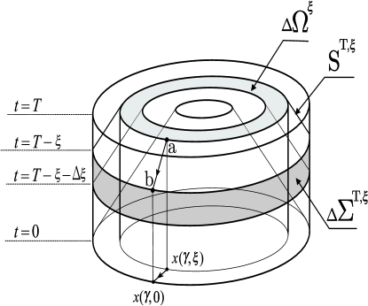
Figure 1: Propagation of jump

$\bullet$   Jumps of $v_{t}(\cdot,T)$ initiate jumps of the velocity $v^{\chi_{\Delta\Omega^{\xi}}y}_{t}$. One of the velocity jumps is located at the characteristic $S^{T,\,\xi}$ . This jump propagates along the space-time rays $r_{\gamma}^{T,\,\xi}$, which constitute the characteristic:

$$r_{\gamma}^{T,\,\xi}:=\{(x,t)\in\overline{\Omega^{T}}\times[0,T]\,|\,\,x=x(\gamma,\xi-\tau),\,\,t=T-\tau:\,\,0\leqslant\xi\leqslant T\}\,,$$

$$S^{T,\,\xi}\,=\,\bigcup_{\gamma\in\Gamma}r_{\gamma}^{T,\,\xi}\,.$$

The jump, which moves along $r_{\gamma}^{T,\,\xi}$, starts from the point $a=(x(\gamma,\xi),T)$ and reaches the boundary at $b=(x(\gamma,0),T-\xi)$. By (4.1), at the ‘input’ $a$ the value (amplitude) of the jump is $y(x(\gamma,\xi))$. At the endpoint $b$, its amplitude is found by the GO-technique, which provides

$$v^{\chi_{\Delta\Omega^{\xi}}y}_{t}(\left(x(\gamma,0),t\right)\bigg{|}_{t=T-\xi-0}^{t=T-\xi+0}=0-\beta^{\frac{1}{2}}(\gamma,\xi)y(x(\gamma,\xi))=-\,\beta^{\frac{1}{2}}(\gamma,\xi)y(x(\gamma,\xi))\,.$$ (4.2)

This relation corresponds to the well-known GO-law: the ratio of the input and output jump amplitudes is governed by the factor $\beta$, which is determined by the spreading of rays $r^{T,\,\xi}_{\gamma}$ [17, 5, 1].

$\bullet$   By the aforesaid, a trace $v^{\chi_{\Delta\Omega^{\xi}}y}_{t}\big{|}_{\Sigma^{T}}$ vanishes on $\Gamma\times(T-\xi,T]$ and has a jump at the cross-section $\Sigma^{T}\cap S^{T,\,\xi}=\Gamma\times\{t=T-\xi\}$. In the mean time, by the regularity results, this trace is continuous as an $H^{\frac{1}{2}}(\Gamma)$-valued function of $t\in[0,T-\xi]$ . The following considerations specify the behavior of $v^{\chi_{\Delta\Omega^{\xi}}y}_{t}\big{|}_{\Sigma^{T}}$ near (and below) this cross-section.

Let

$$\Delta\Sigma^{T,\,\xi}:=\{(\gamma,t)\in\Sigma^{T}\,|\,\,\gamma\in\Gamma,\,\,T-\xi-\Delta\xi\leqslant t\leqslant T-\xi\}$$

be a thin ‘belt’ near the cross-section (see Fig. 1), $\chi_{\Delta\Sigma^{T,\,\xi}}$ its indicator. A function on $\Sigma^{T}$ of the form $\chi_{\Delta\Sigma^{T,\,\xi}}\left[v^{\chi_{\Delta\Omega^{\xi}}y}_{t}\big{|}_{\Sigma^{T}}\right]$ is a ‘slice’ of the boundary trace of the velocity. By (4.2), one can represented it as

$$\left(\chi_{\Delta\Sigma^{T,\,\xi}}\left[v^{\chi_{\Delta\Omega^{\xi}}y}_{t}\big{|}_{\Sigma^{T}}\right]\right)(\gamma,t)\,=$$

$$=\begin{cases}-\beta^{\frac{1}{2}}(\gamma,\xi)y(x(\gamma,\xi))+w^{\xi,\Delta\xi}(\gamma,t)\,,&(\gamma,t)\in\Delta\Sigma^{T,\,\xi}\\ 0\,,&(\gamma,t)\in\Sigma^{T}\setminus\Delta\Sigma^{T,\,\xi}\end{cases}\,\,,$$ (4.3)

where the first summand in the first line does not depend on $t$ and, hence, obeys $\|\beta^{\frac{1}{2}}y\|^{2}_{L_{2}(\Delta\Sigma^{T,\,\xi})}\thicksim\Delta\xi$, whereas the second summand satisfies
$\|w^{\xi,\Delta\xi}\|^{2}_{L_{2}(\Delta\Sigma^{T,\,\xi})}\thicksim o(\Delta\xi)$ uniformly with respect to $\xi\in[0,T]$ and (small enough) $\Delta\xi>0$ [5, 1]. So, the first summand is dominating.

Amplitude integral

$\bullet$   Choose a partition $\Xi=\{\xi_{i}\}_{i=0}^{N}:\,\,\,0=\xi_{0}<\xi_{1}<\dots<\xi_{N}=T$ of the segment $[0,T]$ and denote

$$\Delta\xi_{i}=\xi_{i}-\xi_{i-1}\,,\quad\Delta\Sigma^{T,\,\xi_{i}}=\Gamma\times[T-\xi_{i}-\Delta\xi_{i}\,,T-\xi_{i}]\,,\quad\Delta\Omega^{\xi_{i}}=\overline{\Omega^{\xi_{i}}\setminus\Omega^{\xi_{i-1}}}\,,$$

$$i=1,2,\dots N\,\,\,\,\,\,\,(\Omega^{0}:=\emptyset);\qquad r_{\Xi}\,=\,\max_{i=1,\dots,N}\Delta\xi_{i}\,.$$

Summing up the terms of the form (4.3) and recalling the definition of images, we get

$$\left(\sum\limits_{i=1}^{N}\chi_{\Delta\Sigma^{T,\,\xi_{i}}}\left[v^{\chi_{\Delta\Omega^{\xi_{i}}}y}_{t}\big{|}_{\Sigma^{T}}\right]\right)(\gamma,T-t)\,=$$

$$=\,-\,\left(I^{T}y\right)(\gamma,t)+\delta^{y,\,\Xi}(\gamma,t),\qquad(\gamma,t)\in\Sigma^{T}\,,$$ (4.4)

where $\|\delta^{y,\,\Xi}\|_{L_{2}(\Sigma^{T})}\to 0$ as $r_{\Xi}\to 0$. Substituting $t$ by $T-t$, we see that, for the given smooth $y\in{\cal H}^{T}$, the sums converge to $-Y^{T}I^{T}y$ by the norm in ${\cal F}^{T}$. The smallness of $\delta^{y,\,\Xi}$ is justified by perfect analogy with the case of the problem with Dirichlet boundary controls [5, 1].

$\bullet$   Here we interpret (4.4) in operator terms.

Let $X^{T,\,\xi}$ be a projection in ${\cal F}^{T}$ onto ${\cal F}^{T,\,\xi}$, which cuts off controls onto $\Gamma\times[T-\xi,T]$. The difference $\Delta X^{T,\,\xi_{i}}=X^{T,\,\xi_{i}}-X^{T,\,\xi_{i-1}}$ is also the projection cutting off controls onto the belt $\Delta\Sigma^{\xi_{i},\,T}$: $\Delta X^{T,\,\xi_{i}}f=\chi_{\Delta\Sigma^{T,\,\xi_{i}}}f$.

By $G^{\xi}$ we denote a projection in ${\cal H}^{T}$ onto ${\cal H}^{\xi}$, which cuts off functions onto $\Omega^{\xi}$. The difference $\Delta G^{\xi_{i}}=G^{\xi_{i}}-G^{\xi_{i-1}}$ cuts off functions onto the layer $\Delta\Omega^{\xi_{i}}$: $\Delta G^{\xi_{i}}y=\chi_{\Delta\Omega^{\xi_{i}}}y$.

Recalling the definition of the observation operator, one can represent the summands in (4.4) as

$$\chi_{\Delta\Sigma^{T,\,\xi_{i}}}\left[v^{\chi_{\Delta\Omega^{\xi_{i}}}y}_{t}\big{|}_{\Sigma^{T}}\right]=\Delta X^{T,\,\xi_{i}}\partial_{t}O^{T}\Delta G^{\xi_{i}}y$$

and then write (4.4) in the form

$$\lim\limits_{r_{\Xi}\to 0}\left[\sum\limits_{i=1}^{N}\Delta X^{T,\,\xi_{i}}\partial_{t}O^{T}\Delta G^{\xi_{i}}\right]y=:\left[\int_{[0,T]}dX^{T,\,\xi}\,\partial_{t}O^{T}\,dG^{\xi}\right]y=Y^{T}I^{T}y\,.$$ (4.5)

An operator construction in the square brackets is said to be an amplitude integral (AI). It represents the image of $y$ as a collection of the wave jumps, which pass through $\Omega^{T}$ and are detected by the external observer at the boundary.

$\bullet$   Recall that (4.5) is derived under the assumption $T<T_{c}$. The case $T>T_{c}$ is more complicated since the equidistant surfaces $\Gamma^{\xi}$ can be non-smooth and disconnected. However, a remarkable fact is that representation (4.5) does survive: it is valid for any $T<T_{*}$. For the system $\alpha^{T}$ with Dirichlet boundary controls, this result is stated in [5, 1]. To modify it for the case of Neumann controls requires just a minor technical changes. So, the following does occur.

Proposition 1.

For any positive $T<T_{*}$, the sums in (4.5) converge to the limit

$$\lim\limits_{r_{\Xi}\to 0}\sum\limits_{i=1}^{N}\Delta X^{T,\,\xi_{i}}\partial_{t}O^{T}\Delta G^{\xi_{i}}=:\int_{[0,T]}dX^{T,\,\xi}\,\partial_{t}O^{T}\,dG^{\xi}=Y^{T}I^{T}$$ (4.6)

in the weak operator topology.

$W^{T}$ via amplitude integral

$\bullet$   Multiplying (4.6) by $W^{T}$ from the right, we get an operator $V^{T}:{\cal F}^{T}\to{\cal F}^{T}$,

$$V^{T}:=Y^{T}I^{T}W^{T}=\left[\int_{[0,T]}dX^{T,\,\xi}\,\partial_{t}O^{T}\,dG^{\xi}\right]W^{T},$$ (4.7)

which satisfies

$$V^{T}{\cal F}^{T,\,\xi}\,\subset\,{\cal F}^{T,\,\xi}\,,\qquad(V^{T})^{*}V^{T}\overset{(\ref{C^T triang factor})}{=}C^{T}\,.$$ (4.8)

Thus, $V^{T}$ provides triangular factorization of the connecting operator with respect to the nest $\{{\cal F}^{T,\,\xi}\}_{0\leqslant\xi\leqslant T}$.

$\bullet$    Any densely defined closable linear operator acting from a Hilbert space to a Hilbert space can be represented in the form of a polar decomposition (see, e.g., [10]). For the control operator, such a decomposition is

$$W^{T}\,=\,U^{T}|W^{T}|\,:=\,U^{T}\left[(W^{T})^{*}W^{T}\right]^{\frac{1}{2}}\,\overset{(\ref{C^T triang factor})}{=}\,U^{T}\left[C^{T}\right]^{\frac{1}{2}}\,,$$ (4.9)

where $|W^{T}|:{\cal F}^{T}\to{\cal F}^{T}$ is a modulo of $W^{T}$, and $U^{T}:{\cal F}^{T}\to{\cal H}^{T}$ is an isometry, which maps ${\rm Ran\,}|W^{T}|\subset{\cal F}^{T}$ onto ${\rm Ran\,}W^{T}\subset{\cal H}^{T}$ by the rule

$$U^{T}|W^{T}|f\,=\,W^{T}f\,,\qquad f\in{\cal F}^{T}\,.$$ (4.10)

By (3.10) with $\sigma=\Gamma$, for any $T>0$ one has $\overline{{\rm Ran\,}W^{T}}={\cal H}^{T}$. In the mean time, for $T<T_{*}$, we have

$$\overline{{\rm Ran\,}|W^{T}|}={\cal F}^{T}\ominus{\rm Ker\,}|W^{T}|={\cal F}^{T}\ominus{\rm Ker\,}W^{T}\overset{{\rm Lemma}\,\ref{L1}}{=}{\cal F}^{T}\,.$$

As a result, if $T<T_{*}$ then $U^{T}$ can be extended by continuity from ${\rm Ran\,}|W^{T}|$ to ${\cal F}^{T}$, the extension being a unitary operator, which maps ${\cal F}^{T}$ onto ${\cal H}^{T}$. In what follows, we assume that such an extension is done; it satisfies

$$(U^{T})^{*}U^{T}\,=\,{\mathbb{I}}_{{\cal F}^{T}}\,,\qquad U^{T}(U^{T})^{*}\,=\,{\mathbb{I}}_{{\cal H}^{T}}\,.$$ (4.11)

$\bullet$   Recall that $G^{\xi}$ projects in ${\cal H}^{T}$ onto ${\cal H}^{\xi}$. We say a projection $P^{\xi}$ in ${\cal H}^{T}$ onto the subspace $\overline{W^{T}{\cal F}^{T,\,\xi}}$ (formed by waves) to be a wave projection. A crucial point of our approach is the equality

$$P^{\xi}\,\overset{(\ref{W^T FTxis = Hxis})}{=}\,G^{\xi}\,,\qquad 0\leqslant\xi\leqslant T\,,$$ (4.12)

which corresponds to the controllability of system $\alpha^{T}$.

Let $\tilde{P}^{T,\,\xi}$ be a projection in ${\cal F}^{T}$ onto the subspace $\overline{|W^{T}|{\cal F}^{T,\,\xi}}$. By (4.10), one has

$$U^{T}\tilde{P}^{T,\,\xi}\,=\,P^{\xi}U^{T}\,,\qquad 0\leqslant\xi\leqslant T$$ (4.13)

that implies

$$O^{T}G^{\xi}W^{T}\overset{(\ref{O=W^*}),(\ref{P^xi=G^xi})}{=}(W^{T})^{*}P^{\xi}W^{T}\overset{(\ref{W=U|W|})}{=}|W^{T}|(U^{T})^{*}P^{\xi}U^{T}|W^{T}|=$$

$$\overset{(\ref{U^T tilde P^xi=P^xi})}{=}|W^{T}|\,\tilde{P}^{T,\,\xi}\,|W^{T}|$$ (4.14)

for $0\leqslant\xi\leqslant T$.

$\bullet$   Multiplying equality (4.7) by the isometry $(I^{T})^{*}Y^{T}$ from the left, and taking into account (4.14), we get

$$W^{T}=U^{T}|W^{T}|,\quad U^{T}\,=\,(I^{T})^{*}Y^{T}\left[\int_{[0,T]}dX^{T,\,\xi}\,\partial_{t}|W^{T}|\,d\tilde{P}^{T,\,\xi}\right]\,.$$ (4.15)

Here the operators $I^{T},\,Y^{T},\,X^{T,\,\xi}$ are standard (do not depend on potential $q$), whereas projections $\tilde{P}^{T,\,\xi}$ are obviously determined by $|W^{T}|$. Operator $W^{T}$ is triangular with respect to the pair of the nests $\{{\cal F}^{T,\,\xi}\}$ and $\{{\cal H}^{\xi}\}$ that means $W^{T}{\cal F}^{T,\,\xi}\subset{\cal H}^{\xi},\,\,\,0\leqslant\xi\leqslant T$ (see (3.10)). From the operator theory viewpoint, representation (4.15) enables one to recover a triangular operator $W^{T}$ via its modulo $|W^{T}|$, the ‘phase’ part $U^{T}$ being expressed via a relevant operator integral. The integral into the square brackets is referred to as a diagonal of operator $\partial_{t}W^{T}$ with respect to the nests $\{{\cal F}^{T,\,\xi}\}$ and $\{{\cal H}^{\xi}\}$ [12, 9].

$\bullet$   Introduce an operator $A^{T}:{\cal F}^{T}\to{\cal F}^{T}$ by

$$A^{T}\,:=\,Y^{T}\int_{[0,T]}dX^{T,\,\xi}\,\partial_{t}[C^{T}]^{\frac{1}{2}}\,d\tilde{P}^{T,\,\xi}\,.$$ (4.16)

With regard to (4.12) and (4.13), one can write (4.6) in the form $A^{T}(U^{T})^{*}=I^{T}$ that enables one to represent the phase operator in the form

$$U^{T}\overset{(\ref{W^T=U^T|W^T|})}{=}(I^{T})^{*}A^{T}\,.$$

By (4.11) and (2.3), this representation implies

$$\quad(A^{T})^{*}A^{T}\,=\,{\mathbb{I}}_{{\cal F}^{T}},\qquad A^{T}(A^{T})^{*}\,=\,G_{\Theta^{T}}\,.$$ (4.17)

Now, writing (4.15) in the form

$$W^{T}\,=\,(I^{T})^{*}A^{T}\,[C^{T}]^{\frac{1}{2}}\,,$$ (4.18)

we obtain the representation of the control operator, which plays a basic role in solving inverse problems. The reason is the following.

Operator $R^{2T}$ formalizes information, which the external observer gets from measurements at the boundary $\Gamma$. The waves $u^{f}$ propagate into $\Omega$ and are invisible for him. However, the observer can determine $C^{T}$ via (3.19), find $[C^{T}]^{\frac{1}{2}}$, construct the integral (4.16), determine $W^{T}$ via (4.18), and eventually recover invisible waves $u^{f}(\cdot,T)=W^{T}f$. In the BC-method, such a remarkable option is referred to as a visualization of waves.

4.2 Solving the inverse problem

Setup

As is mentioned in section 3.2, the extended response operator $R^{2T}$ depends on the potential locally: it is determined by $q\big{|}_{\Omega^{T}}$. Such a locality motivates the following setup of the inverse problem.

(IP)   Given operator $R^{2T}$, to recover potential $q$ in the subdomain $\Omega^{T}$.

The IP will be solved for an arbitrary fixed $T<T_{*}$. Surely, such an option enables one to determine $q$ in the whole $\Omega$ if $R^{2T}$ is given for a $T\geqslant T_{*}$.

Procedure

Preparatory to solving the IP, recall that geometry of the wave propagation in system $\alpha^{T}$ is governed by the leading part $\partial^{2}_{t}-\Delta$ of the wave equation (3.1). Since this part does not depend on the potential, the geometry is Euclidean. Therefore, we have the right to regard all the geometric objects and parameters ($\Omega^{\xi}$, sgc, $\Theta^{T}$, $\beta$, $T_{*}$, etc) as known and use them for determination of $q$. In particular, we can use the image operator $I^{T}$.

Let $T<T_{*}$ be fixed. Given $R^{2T}$ one can recover $q$ in $\Omega^{T}$ by the following procedure.

Step 1.   Find $C^{T}$ by (3.19). Determine $[C^{T}]^{\frac{1}{2}}$.

Step 2.   Determine the subspaces $[C^{T}]^{\frac{1}{2}}{\cal F}^{T,\,\xi}$ and the corresponding projections $\tilde{P}^{T,\,\xi}$ for $0\leqslant\xi\leqslant T$.

Step 3.   Construct the integral (4.16) and, then, recover $W^{T}$ via (4.18).

Step 4.   Determine $q\big{|}_{\Omega^{T}}$ from the graph (3.11).

The IP is solved.

4.3 Characterization of data

Main result

In addition to the procedure, which solves the IP, we provide the necessary and sufficient conditions for its solvability.

Theorem 1.

Let $0<T<T_{*}$. An operator ${\cal R}^{2T}:{\cal F}^{2T}\to{\cal F}^{2T}$ is the extended response operator of a system $\alpha^{T}$ with potential of the class $L_{\infty}(\Omega^{T})$ if and only if it satisfies the following conditions:

1. ${\cal R}^{2T}$ is a compact operator obeying

   $$Y^{2T}{\cal R}^{2T}=({\cal R}^{2T}Y^{2T})^{*};\,\,\,{\cal R}^{2T}{\cal T}^{2T}_{2T-\xi}={\cal T}^{2T}_{2T-\xi}{\cal R}^{2T},\quad 0\leqslant\xi\leqslant 2T\,.$$ (4.19)

2. An operator ${\cal C}^{T}:{\cal F}^{T}\to{\cal F}^{T}$,

   $${\cal C}^{T}\,:=\,-\,\frac{1}{2}\,(S^{T})^{*}{\cal R}^{2T}J^{2T}S^{T}$$ (4.20)

   is symmetric and positive: $({\cal C}^{T}f,f)_{{\cal F}^{T}}>0$ for $0\not=f\in{\cal F}^{T}$.

3. Let $\tilde{\cal P}^{T,\,\xi}$ be a projection in ${\cal F}^{T}$ onto $\overline{[{\cal C}^{T}]^{\frac{1}{2}}{\cal F}^{T,\,\xi}}$. An operator integral ${\cal A}^{T}:{\cal F}^{T}\to{\cal F}^{T}$,

   $${\cal A}^{T}\,:=\,Y^{T}\int_{[0,T]}dX^{T,\,\xi}\,\partial_{t}[{\cal C}^{T}]^{\frac{1}{2}}\,d\tilde{\cal P}^{T,\,\xi}$$ (4.21)

   converges in the weak operator topology to an isometry, which satisfies

   $$({\cal A}^{T})^{*}{\cal A}^{T}\,=\,{\mathbb{I}}_{{\cal F}^{T}},\quad{\cal A}^{T}({\cal A}^{T})^{*}\,=\,G_{\Theta^{T}}\,.$$ (4.22)

4. An operator ${\cal W}^{T}:{\cal F}^{T}\to{\cal H}^{T}$

   $${\cal W}^{T}\,:=\,(I^{T})^{*}{\cal A}^{T}[{\cal C}^{T}]^{\frac{1}{2}}$$ (4.23)

   satisfies ${\cal W}^{T}{\cal M}^{T}\subset H^{2}(\Omega^{T})$.

5. The relation

   $$\partial_{\nu}{\cal W}^{T}f\big{|}_{\Gamma}\,=\,f(\cdot,T)\,,\qquad f\in{\cal M}^{T}$$ (4.24)

   is valid.

6. The relation

   $$\overline{{\cal W}^{T}{\cal F}^{T,\,\xi}_{\sigma}}\,=\,{\cal H}^{\xi}_{\sigma}\,,\qquad 0\leqslant\xi\leqslant T$$ (4.25)

   holds for any open $\sigma\subseteq\Gamma$.

7. The relation

   $$\sup\limits_{0\not=f\in{\cal M}^{T}}\frac{\|\Delta{\cal W}^{T}f-{\cal W}^{T}f_{tt}\|_{{\cal H}^{T}}}{\|{\cal W}^{T}f\|_{{\cal H}^{T}}}\,<\,\infty$$ (4.26)

   holds.

The proof consists of two parts.

Part I (necessity)

$\square$   Let ${\cal R}^{2T}=R^{2T}$, where $R^{2T}$ is the extended response operator of a system $\alpha^{T}$ with potential $q\in L_{\infty}(\Omega^{T})$. The system possesses the connecting, control, and phase operators $C^{T}$, $W^{T}$, and $U^{T}$ respectively.

1.   Relations (4.19) hold by (3.16).

$\it 2.$    In view of (3.19), operator ${\cal C}^{T}$ defined by (4.20) coincides with $C^{T}$, which is a compact positive operator.

$\it 3.$   The equality ${\cal C}^{T}=C^{T}$ implies $\tilde{\cal P}^{T,\,\xi}=\tilde{P}^{T,\,\xi}$. Comparing (4.16) with (4.21), we conclude that ${\cal A}^{T}=A^{T}$. Hence, (4.22) follows from (4.17).

$\it 4.$    Comparing (4.23) with (4.18), we see that ${\cal W}^{T}$ coincides with $W^{T}$. Hence, ${\cal W}^{T}{\cal M}^{T}\subset H^{2}(\Omega^{T})$ holds by the regularity results on the problem (3.1)–(3.3) (see section 3.1).

$\it 5.$   Since ${\cal W}^{T}=W^{T}$, the equality (4.24) is just a form of writing (3.7).

$\it 6.$   (4.25) holds by (3.10).

$\it 7.$   Since ${\cal W}^{T}f=W^{T}f=u^{f}(\cdot,T)$, we have

$$-\Delta{\cal W}^{T}f+{\cal W}^{T}f_{tt}=-\Delta u^{f}(\cdot,T)+u^{f_{tt}}(\cdot,T)\overset{(\ref{Delay rel})}{=}$$

$$=-\Delta u^{f}(\cdot,T)+u^{f}_{tt}(\cdot,T)\,\overset{(\ref{B1})}{=}\,qu^{f}(\cdot,T)\,.$$

The inequality (4.26) is a consequence of $q\in L_{\infty}(\Omega^{T})$.    $\blacksquare$

Part II (sufficiency)

The proof of sufficiency is constructive: given ${\cal R}^{2T}$ we provide a system $\alpha^{T}$ with the response operator $R^{2T}={\cal R}^{2T}$. In fact, the construction follows the procedure Step 1-4, which solves the IP.

$\square$   Assume that ${\cal R}^{2T}$ obeys $\it 1$-$\it 5$.

$\bullet$    Determine operator ${\cal C}^{T}$ by (4.20) and find $[{\cal C}^{T}]^{\frac{1}{2}}$. The latter is also positive and injective.

Construct the operator integral in (4.21) and get operator ${\cal A}^{T}$. By (4.22), ${\cal A}^{T}$ is an isometry in ${\cal F}^{T}$ with the range $G_{\Theta^{T}}{\cal F}^{T}$. Hence, it satisfies $G_{\Theta^{T}}{\cal A}^{T}={\cal A}^{T}$.

Introduce operator ${\cal W}^{T}:{\cal F}^{T}\to{\cal H}^{T}$ in accordance with (4.23). Obviously, it is injective. By (4.25) (for $\xi=T$ and $\sigma=\Gamma$), its range ${\cal W}^{T}{\cal F}^{T}$ is dense in ${\cal H}^{T}$. Also, it satisfies

$$({\cal W}^{T})^{*}{\cal W}^{T}=[{\cal C}^{T}]^{\frac{1}{2}}({\cal A}^{T})^{*}I^{T}(I^{T})^{*}{\cal A}^{T}[{\cal C}^{T}]^{\frac{1}{2}}\overset{(\ref{I^T properties})}{=}[{\cal C}^{T}]^{\frac{1}{2}}({\cal A}^{T})^{*}G_{\Theta^{T}}{\cal A}^{T}[{\cal C}^{T}]^{\frac{1}{2}}=$$

$$=[{\cal C}^{T}]^{\frac{1}{2}}({\cal A}^{T})^{*}{\cal A}^{T}[{\cal C}^{T}]^{\frac{1}{2}}\,\overset{(\ref{A^T* A^T=1})}{=}\,{\cal C}^{T}\,.$$ (4.27)

$\bullet$   Since ${\cal W}^{T}$ is injective, the set of pairs $\left\{\langle{\cal W}^{T}f,\,{\cal W}^{T}f_{tt}\rangle\,|\,\,f\in{\cal M}^{T}\right\}$ constitutes the graph of a linear operator acting in ${\cal H}^{T}$. This operator is denoted by $L^{T}:{\cal W}^{T}f\mapsto{\cal W}^{T}f_{tt}$. It acts in ${\cal H}^{T}$ and is densely defined (on ${\cal W}^{T}{\cal F}^{T}$).

Recall that the class of smooth controls ${\cal M}^{T}$ is dense in ${\cal F}^{T}$, its elements vanishing near $t=0$. The subclass

$${\cal M}^{T}_{0}:=\{f\in{\cal M}^{T}\,|\,\,f\,\,{\rm vanishes\,\,near\,\,}t=T\}$$

is also dense in ${\cal F}^{T}$. Hence, ${\cal W}^{T}{\cal M}^{T}_{0}$ is dense in ${\cal H}^{T}$ by (4.25) for $\sigma=\Gamma,\,\xi=T$. As a result, an operator $L^{T}_{0}:=L^{T}\big{|}_{{\cal W}^{T}{\cal M}^{T}_{0}}$ is densely defined in ${\cal H}^{T}$. Show that it is symmetric.

Take $f,g\in{\cal M}^{T}_{0}$. Note that $S^{T}f$ and $S^{T}g$ are twice differentiable with respect to $t$ and vanish near $t=0$ and $t=2T$. Also, note that the second relation in (4.19) implies the commutation ${\cal R}^{2T}\partial^{2}_{t}=\partial^{2}_{t}{\cal R}^{2T}$. Then, we have

$$(L^{T}_{0}{\cal W}^{T}f,{\cal W}^{T}g)_{{\cal H}^{T}}=(L^{T}{\cal W}^{T}f,{\cal W}^{T}g)_{{\cal H}^{T}}=({\cal W}^{T}f_{tt},{\cal W}^{T}g)_{{\cal H}^{T}}\overset{(\ref{{cal W}^*{cal W}= cal C})}{=}$$

$$=({\cal C}^{T}f_{tt},g)_{{\cal F}^{T}}\overset{(\ref{cal C^T})}{=}-\,\frac{1}{2}\,([{\cal R}^{2T}J^{2T}S^{T}]f_{tt},S^{T}g)_{{\cal F}^{2T}}=$$

$$=-\,\frac{1}{2}\,([{\cal R}^{2T}J^{2T}S^{T}f]_{tt},S^{T}g)_{{\cal F}^{2T}}\overset{\star}{=}-\,\frac{1}{2}\,({\cal R}^{2T}J^{2T}S^{T}f,[S^{T}g]_{tt})_{{\cal F}^{2T}}=$$

$$=-\,\frac{1}{2}\,({\cal R}^{2T}J^{2T}S^{T}f,S^{T}g_{tt})_{{\cal F}^{2T}}=-\,\frac{1}{2}\,((S^{T})^{*}{\cal R}^{2T}J^{2T}S^{T}f,g_{tt})_{{\cal F}^{T}}=$$

$$=({\cal C}^{T}f,g_{tt})_{{\cal F}^{T}}\overset{(\ref{{cal W}^*{cal W}= cal C})}{=}({\cal W}^{T}f,{\cal W}^{T}g_{tt})_{{\cal H}^{T}}=({\cal W}^{T}f,L^{T}{\cal W}^{T}g)_{{\cal H}^{T}}=$$

$$=({\cal W}^{T}f,L^{T}_{0}{\cal W}^{T}g)_{{\cal H}^{T}}.$$

In $(\star)$ we integrate by part with respect to time in ${\cal F}^{T}=L_{2}(\Sigma^{T})$. So, $L^{T}_{0}$ is symmetric.

$\bullet$    Owing to (4.26), operator $Q^{T}:=\Delta-L^{T}$ defined on the dense set ${\cal W}^{T}{\cal F}^{T}\subset{\cal H}^{T}$, is bounded. By this, we assume that $Q^{T}$ is extended to ${\cal H}^{T}$ by continuity.

Operator $Q^{T}$ is self-adjoint. Indeed, in view of (4.24), for $f\in{\cal M}^{T}_{0}$ one has $\partial_{\nu}{\cal W}^{T}f\big{|}_{\Gamma}=f\big{|}_{t=T}=0$, i.e., elements of ${\cal W}^{T}{\cal M}^{T}_{0}$ satisfy the homogeneous Neumann boundary condition on $\Gamma$. By the latter, the Laplacian $\Delta$ is symmetric on ${\cal W}^{T}{\cal M}^{T}_{0}$. Hence, $Q^{T}\big{|}_{{\cal W}^{T}{\cal M}^{T}_{0}}=\Delta\big{|}_{{\cal W}^{T}{\cal M}^{T}_{0}}-L^{T}_{0}$ is symmetric on a dense set. Since it is bounded, we conclude that $(Q^{T})^{*}=Q^{T}$.

$\bullet$   For $f\in{\cal M}^{T}\subset{\cal F}^{T}$, define a function

$$u^{f}(x,t)\,:=\,\left({\cal W}^{T}{\cal T}^{T}_{T-t}f\right)(x)\qquad{\rm in}\,\,\,\overline{\Omega^{T}}\times[0,T]\,.$$ (4.28)

The definitions of the operators imply

$$\left[\Delta-Q^{T}\right]u^{f}(\cdot,t)=L^{T}u^{f}(\cdot,t)=L^{T}{\cal W}^{T}{\cal T}^{T}_{T-t}f={\cal W}^{T}\left[{\cal T}^{T}_{T-t}f\right]_{tt}=$$

$$=[{\cal W}^{T}{\cal T}^{T}_{T-t}f]_{tt}\,=\,u^{f}_{tt}(\cdot,t)\,.$$

Thus, $u^{f}$ satisfies the equation

$$u_{tt}-\Delta u+Q^{T}u\,=\,0\qquad{\rm in}\,\,\,\Omega^{T}\times(0,T)\,,$$ (4.29)

By (4.25) for $\sigma=\Gamma$, we have $\rm supp\,u^{f}(\cdot,t)\subset\overline{\Omega^{t}}$, i.e., $u^{f}$ satisfies the Cauchy condition

$$u\big{|}_{t<\tau(x)}=0\qquad{\rm in}\,\,\,\overline{\Omega^{T}}\times[0,T]\,.$$ (4.30)

In the mean time, (4.24) easily implies that $u^{f}$ obeys

$$\partial_{\nu}u=f\qquad{\rm on}\,\,\,\overline{\Sigma^{T}}\,.$$ (4.31)

$\bullet$    Show that $Q^{T}$ is a multiplication by bounded function. The proof follows the idea of [4].

Lemma 3.

There is a (real) function $q\in L_{\infty}(\Omega^{T})$ such that $Q^{T}y=qy$ holds for $y\in{\cal H}^{T}$.

$\square$   1. Choose a $\sigma\subset\Gamma$ and $f\in{\cal F}^{T,\,\xi}_{\sigma}\cap{\cal M}^{T}$. By condition 4 and (4.25), we have $u^{f}(\cdot,T)\in{\cal H}^{\xi}_{\sigma}\cap H^{2}(\Omega^{T})$. Hence, $\Delta u^{f}(\cdot,T)\in{\cal H}^{\xi}_{\sigma}$. In the mean time, we have $f_{tt}\in{\cal F}^{T,\,\xi}_{\sigma}\cap{\cal M}^{T}$ that implies $u^{f}_{tt}=L^{T}u^{f}(\cdot,T)={\cal W}^{T}f_{tt}\,\overset{(\ref{cal W^T new})}{\in}\,{\cal H}^{\xi}_{\sigma}$. Therefore, $Q^{T}u^{f}(\cdot,T)\overset{(\ref{E1})}{=}\Delta u^{f}(\cdot,T)-u^{f}_{tt}\in\,{\cal H}^{\xi}_{\sigma}$. Thus, $Q^{T}{\cal W}^{T}{\cal F}^{T,\,\xi}_{\sigma}\subset{\cal H}^{\xi}_{\sigma}$ holds. Since ${\cal W}^{T}{\cal F}^{T,\,\xi}_{\sigma}$ is dense in ${\cal H}^{\xi}_{\sigma}$ (see (4.25)), we conclude that $Q^{T}{\cal H}^{\xi}_{\sigma}\subset{\cal H}^{\xi}_{\sigma}$. The latter leads to $Q^{T}[{\cal H}^{T}\ominus{\cal H}^{\xi}_{\sigma}]\subset[{\cal H}^{T}\ominus{\cal H}^{\xi}_{\sigma}]$ by virtue of the symmetry $(Q^{T})^{*}=Q^{T}$. Hence, the subspaces ${\cal H}^{\xi}_{\sigma}$ reduce $Q^{T}$ that is equivalent to the commutation

$$Q^{T}G^{\xi}_{\sigma}\,=\,G^{\xi}_{\sigma}Q^{T}\,,\,\,\,\qquad\sigma\subset\Gamma,\,\,\,\,0\leqslant\xi\leqslant T\,,$$ (4.32)

where $G^{\xi}_{\sigma}$ projects in ${\cal H}^{T}$ onto ${\cal H}^{\xi}_{\sigma}$, i.e., cuts off functions on $\Omega^{\xi}_{\sigma}$.

2. As is easy to verify, an operator $\tau^{T}_{\sigma}:{\cal H}^{T}\to{\cal H}^{T}$,

$$\tau^{T}_{\sigma}y:=\left[\int_{[0,T]}\xi\,dG^{\xi}_{\sigma}\right]y=\left[\lim\limits_{r_{\Xi}\to 0}\sum\limits_{i=1}^{N}\xi_{i}\,[G^{\xi_{i}}_{\sigma}-G^{\xi_{i-1}}_{\sigma}]\right]y$$ (4.33)

(the sums converge by the operator norm) acts by the rule

$$\tau^{T}_{\sigma}y=\begin{cases}{\rm d}(\cdot,\sigma)y&{\rm in}\,\,\,\Omega^{T}_{\sigma}\\ 0&{\rm in}\,\,\,\Omega^{T}\setminus\Omega^{T}_{\sigma}\\ \end{cases}\,,$$

i.e., multiplies functions by the distance to $\sigma$ and, then, cuts off on $\Omega^{T}_{\sigma}$ [4]. As a consequence, an operator

$$\hat{\tau}^{T}_{\sigma}\,:=\,\tau^{T}_{\sigma}y\,+\,T({\mathbb{I}}_{{\cal H}^{T}}-G^{T}_{\sigma})y$$

multiplies functions by the continuous function ${\rm d}^{T}_{\sigma}(\cdot):=\max\{{\rm d}(\cdot,\sigma),T\}$. In the mean time, (4.32) implies

$$Q^{T}\hat{\tau}^{T}_{\sigma}\,=\,\hat{\tau}^{T}_{\sigma}Q^{T}\,,\qquad\sigma\subset\Gamma,\,\,\,\,0\leqslant\xi\leqslant T\,,$$ (4.34)

because the sums in (4.33) do commute with all $G^{\xi}_{\sigma}$.

3.  Fix a (small) $\delta>0$. A simple geometric fact is that the functions $\{{\rm d}^{T}_{\sigma}\,|\,\,\sigma\subset\Gamma\}$ separate points in $\Omega^{T-\delta}$ and vanish simultaneously in no point $x_{0}\in\overline{\Omega^{T-\delta}}$. Hence, a family $\{{\rm d}^{T}_{\sigma}\,|\,\,\sigma\subset\Gamma,\,\,0\leqslant\xi\leqslant T\}$ generates the continuous function algebra $C(\overline{\Omega^{T-\delta}})$ [4].

Correspondingly, an operator family $\{\hat{\tau}^{T}_{\sigma}\,|\,\,\sigma\subset\Gamma,\,\,0\leqslant\xi\leqslant T\}$ generates the operator (sub)algebra ${\mathfrak{C}}(\overline{\Omega^{T-\delta}})\subset{\mathfrak{B}}({\cal H}^{T})$ of multiplications by continuous functions. As a consequence of (4.34), we have $Q^{T}{\mathfrak{C}}(\overline{\Omega^{T-\delta}})={\mathfrak{C}}(\overline{\Omega^{T-\delta}})Q^{T}$ that is possible if and only if $Q^{T}$ is also a multiplication by a function $q$.

Since $Q^{T}$ is bounded, we have $q\in L_{\infty}(\Omega^{T-\delta})$. By arbitrariness of $\delta$, we get $q\in L_{\infty}(\Omega^{T})$.    $\blacksquare$

$\bullet$   With the above determined function $q$ one associates the system $\alpha^{T}$ of the form (3.5)–(3.7). Such a system possesses its own operators $W^{T}$ and $C^{T}$. Show that $W^{T}={\cal W}^{T}$ and $C^{T}={\cal C}^{T}$.

Since the problems (3.5)–(3.7) and (4.29)–(4.31) (with $Q^{T}=q$) are identical and uniquely solvable, their solutions (for the same $f$’s) coincide. Writing the first relation of (3.8) in the form $u^{f}(\cdot,t)=W^{T}{\cal T}^{T}_{T-t}f$ and comparing with (4.28), we see that $W^{T}={\cal W}^{T}$ holds.

By the latter equality and (4.27), we have

$${\cal C}^{T}\,=\,({\cal W}^{T})^{*}{\cal W}^{T}\,=\,(W^{T})^{*}W^{T}\,=\,C^{T}\,.$$ (4.35)

$\bullet$   System (4.29)–(4.31) (with $Q^{T}=q$) possesses the extended response operator $R^{2T}$. Here we prove the equality $R^{2T}={\cal R}^{2T}$ that completes the proof of the Theorem.

Begin with two lemmas of general character. The lemmas deal with a Hilbert space ${\cal F}=L_{2}([0,2T];\,{\cal E})$ (with the Lebesgue measure $dt$), where $\cal E$ is an auxiliary Hilbert space. By ${\cal F}_{\pm}$ we denote the subspaces of functions, which are even and odd with respect to $t=T$. So, the decompositions ${\cal F}\,=\,{\cal F}_{+}\oplus{\cal F}_{-}$ holds. Let

$${\cal F}^{[a,b]}\,:=\,\{f\in{\cal F}\,|\,\,\rm supp\,f\subset[a,b]\}\,,\qquad 0\leqslant a<b\leqslant 2T\,.$$

Lemma 4.

If a bounded operator $N:{\cal F}\to\cal F$ satisfies

$$N{\cal F}_{\pm}\,\subset\,{\cal F}_{\pm}\,;\quad N{\cal F}^{[a,2T]}\,\subset\,{\cal F}^{[a,2T]}\,,\,\,\,0\leqslant a\leqslant 2T$$ (4.36)

then it is local, i.e., preserves the support of functions:

$$N{\cal F}^{[a,b]}\,\subset\,{\cal F}^{[a,b]}\,,\qquad 0\leqslant a<b\leqslant 2T\,.$$ (4.37)

$\square$       1.  Representing ${\cal F}={\cal F}^{[0,T]}\oplus{\cal F}^{[T,2T]}$ and $f=f_{1}+f_{2}$ with $f_{1}\in{\cal F}^{[0,T]},\,f_{2}\in{\cal F}^{[T,2T]}$, we identify $f\equiv\langle f_{1},f_{2}\rangle$.

Introduce an isometry $Y:{\cal F}^{[0,T]}\to{\cal F}^{[T,2T]}$ by

$$(Yf)(t)\,:=\,f(2T-t)\,,\qquad T\leqslant t\leqslant 2T\,.$$

Obviously, one has ${\cal F}_{\pm}=\{\langle f,\pm Yf\rangle\}\,|\,\,f\in{\cal F}^{[0,T]}\}$. Since $N$ preserves the evenness/oddness, there are two operators $k,l:{\cal F}^{[0,T]}\to{\cal F}^{[0,T]}$ such that

$$N\langle f,Yf\rangle=\langle kf,Ykf\rangle\qquad{\rm and}\qquad N\langle f,-Yf\rangle=\langle lf,-Ylf\rangle\,.$$ (4.38)

Show that $k=l$. For a $g\in{\cal F}^{[0,T]}$, one has

$$2N\langle 0,Yg\rangle=N\left[{\langle g,Yg\rangle-\langle g,-Yg\rangle}\right]\overset{(\ref{Aux 1})}{=}\langle kg,Ykg\rangle-\langle lg,-Ylg\rangle=$$

$$=\langle[k-l]g,Y[k+l]g\rangle\,.$$ (4.39)

In the mean time, we have $\langle 0,Yg\rangle\in{\cal F}^{[T,2T]}$ and, hence, $N\langle 0,Yg\rangle\in{\cal F}^{[T,2T]}$ holds by (4.36). By the latter, $2N\langle 0,Yg\rangle$ must be of the form $\langle 0,...\rangle$, i.e., $[k-l]g=0$ is valid and implies $k=l=:m$.

2.   Putting $g=Y^{-1}h$ in (4.39), we get

$$N\langle 0,h\rangle\,=\,\langle 0,YmY^{-1}h\rangle\,.$$ (4.40)

In the mean time, we have

$$2N\langle g,0\rangle=N\left[{\langle g,Yg\rangle+\langle g,-Yg\rangle}\right]\overset{(\ref{Aux 1})}{=}\langle mg,Yg\rangle+\langle mg,-Ymg\rangle=$$

$$=\,2\langle mg,0\rangle\,.$$

Combining the latter with (4.40), we arrive at the representation

$$N\langle g,h\rangle\,=\,\langle mg,YmY^{-1}h\rangle\,.$$ (4.41)

3.   Such a representation easily provides the following fact: operator $N$ acts locally in $[0,2T]$ if and only if operator $m$ is local in $[0,T]$. Show that the latter does occur.

Let ${\rm supp\,}f\subset[a,b]\subset[0,T]$, so that $f\big{|}_{0\leqslant t<a}=0\qquad{\rm and}\qquad f\big{|}_{b<t\leqslant 2T}=0$ holds. The first equality means that $f\in{\cal F}^{[a,2T]}$, implies $Nf\in{\cal F}^{[a,2T]}$ by (4.36) and, thus, provides $Nf\big{|}_{0\leqslant t<a}=0$. Hence, with regard to $f\equiv\langle f,0\rangle$, we have

$$0=Nf\big{|}_{0\leqslant t<a}\equiv\left[N\langle f,0\rangle\right]\big{|}_{0\leqslant t<a}\overset{(\ref{Aux 4})}{=}\langle mf,0\rangle\big{|}_{0\leqslant t<a}\equiv mf\big{|}_{0\leqslant t<a}\,,$$

i.e., $m$ does not extend support to the left.

By the choice of $f$, one has ${\rm supp\,}Yf\subset[2T-b,2T-a]$, so that $Yf\in{\cal F}^{[2T-b,2T]}$. The latter implies $NYf\in{\cal F}^{[2T-b,2T]}$ in accordance with (4.36). Hence, we have

$$0=NYf\big{|}_{0\leqslant t<2T-b}\equiv\left[N\langle 0,Yf\rangle\right]\big{|}_{0\leqslant t<2T-b}\overset{(\ref{Aux 4})}{=}\langle 0,Ymf\rangle\big{|}_{0\leqslant t<2T-b}\equiv$$

$$\equiv\,Ymf\big{|}_{0\leqslant t<2T-b}\,.$$

Therefore, $mf\big{|}_{t>2T-b}=0$, i.e., $m$ does not extend support to the right. Thus, $m$ acts locally and, eventually, $N$ is local.     $\blacksquare$

In fact, the boundedness of $N$ is not substantial and the proof (mutatis mutandis) is available for a wider class of operators.

Lemma 5.

If an operator $N$ satisfies (4.36) and is compact then $N=\mathbb{O}$.

$\square$    A projection $X^{[a,b]}$ in $\cal F$ onto ${\cal F}^{[a,b]}$ cuts off functions on $[a,b]$. The complement projection $X^{[a,b]}_{\bot}={\mathbb{I}}-X^{[a,b]}$ cuts off on $[0,a]\cup[b,2T]$. By Lemma 4, we have

$$NX^{[a,b]}=X^{[a,b]}NX^{[a,b]}\quad{\rm and}\quad NX^{[a,b]}_{\bot}=X^{[a,b]}_{\bot}NX^{[a,b]}_{\bot}\,.$$

Summing up, we get $N=X^{[a,b]}NX^{[a,b]}+X^{[a,b]}_{\bot}NX^{[a,b]}_{\bot}$ that leads to

$$NX^{[a,b]}=X^{[a,b]}N\,,\qquad N^{*}X^{[a,b]}=X^{[a,b]}N^{*}$$

and, eventually, implies

$$N^{*}NX^{[a,b]}\,=\,X^{[a,b]}N^{*}N\,.$$ (4.42)

In the mean time, operator $N^{*}N$ is self-adjoint and compact. Let $\lambda\in\mathbb{R}$ be its eigenvalue, ${\cal D}_{\lambda}$ the corresponding eigensubspace. By (4.42), we have $X^{[a,b]}{\cal D}_{\lambda}\subset{\cal D}_{\lambda}$ that leads to ${\rm dim\,}{\cal D}_{\lambda}=\infty$. The latter is possible only for ${\cal D}_{0}={\rm Ker\,}N^{*}N$. Thus, the spectrum of $N^{*}N$ is exhausted by $\lambda=0$. Hence, $N^{*}N=\mathbb{O}$. Therefore, $N=\mathbb{O}$.      $\blacksquare$

$\bullet$   Now, we are ready to complete the proof of Theorem 1. Return to our system (4.29)–(4.31) (with $Q^{T}=q$). Recall that $S^{T}:{\cal F}^{T}\to{\cal F}^{2T}$ extends controls from $[0,T]$ to $[0,2T]$ by oddness with respect to $t=T$. We regard ${\cal F}^{2T}=L_{2}(\Sigma^{2T})$ as the space $L_{2}([0,2T];{\cal E})$ with ${\cal E}=L_{2}(\Gamma)$. Let ${\cal F}^{2T}_{\pm}$ be the subspaces of the even and odd functions, so that the decomposition

$${\cal F}^{2T}\,=\,{\cal F}^{2T}_{+}\oplus{\cal F}^{2T}_{-}$$

occurs. The embedding $J^{2T}{\cal F}^{2T}_{-}\subset{\cal F}^{2T}_{+}$ holds and is dense. Also, one has $Y^{2T}{\cal F}^{2T}_{\pm}={\cal F}^{2T}_{\pm}$.

Denote $N:=R^{2T}-{\cal R}^{2T}$ With regard to (3.19) and (4.20), the equality (4.35) leads to

$$(NJ^{2T}S^{T}f,S^{T}g)_{{\cal F}^{2T}}=0$$

for all $f,g\in{\cal F}^{T}$. It shows that the embedding

$$N{\cal F}^{2T}_{+}\,\subset\,{\cal F}^{2T}_{+}$$

holds and evidently implies $Y^{2T}N{\cal F}^{2T}_{+}\,\subset\,{\cal F}^{2T}_{+}$. In the mean time, operator $Y^{2T}N$ is self-adjoint: see (3.16) and (4.19). Therefore, it is reduced by the even/odd subspaces: $Y^{2T}N{\cal F}^{2T}_{\pm}\,\subset\,{\cal F}^{2T}_{\pm}$. The latter leads to

$$N{\cal F}^{2T}_{\pm}\,\subset\,{\cal F}^{2T}_{\pm}\,.$$ (4.43)

On the other hand, the shift invariance (3.16) and (4.19) implies

$$N{\cal F}^{2T,\,\xi}\,\subset{\cal F}^{2T,\,\xi}\,,\qquad 0\leqslant\xi\leqslant 2T\,.$$ (4.44)

Joining (4.43) with (4.44) and applying Lemma 5, we arrive at $N=\mathbb{O}$ that is $R^{2T}={\cal R}^{2T}$. Theorem 1 is proved.    $\blacksquare$

5 Comments, doubts, philosophy

$\bullet$   A characterization of data for an inverse problem is a list of conditions providing its solvability. The reasonable requirement to any characterization is to be checkable and possibly simple. As we guess, the only reasonable understanding of ‘a condition is checkable’ is that it can be verified before (without) solving the inverse problem. Formally, the conditions 1–7 of Theorem 1 satisfy such a requirement because they do not use the knowledge of the potential $q$. However, comparing these conditions with the procedure Step 1–4, it is easy to recognize that to check 1–7 is almost the same as to recover $q$. Conditions 1–7 just provide the procedure to be realizable. In such a situation, can one claim that 1–7 is an efficient characterization?

And what is ‘efficient’? For instance, the key step of the procedure, as well as the characterization, is constructing the operator integral (4.21). If it is at our disposal, we get $W^{T}$, recover the waves $u^{f}$, and are able to check 5–7. In the mean time, having $u^{f}$ one doesn’t need to check anything more but can just determine $q$ from the wave equation. So, can one regard the required in 3 convergence as an efficiently checkable condition? We don’t have a convincible answer.

Also, can one avoid so long list of conditions and invent something simpler and better? We are rather sceptical and the following is some reasons for scepticism.

$\bullet$   The evolution of system (3.5)–(3.7) is governed by the operator $L_{q}=-\Delta+q$ and Neumann controls $f=\partial_{\nu}u\big{|}_{\Sigma^{T}}$. Both of them are of very specific type. We mean, replacing them by $L_{Q}=-\sum_{i,j}\partial_{x_{i}}a^{ij}\partial_{x^{j}}+Q$ (with possibly nonlocal and time dependent $Q$) and, let say, $f=[\partial_{\nu}u+\varkappa u]\big{|}_{\Sigma^{T}}$, we’d got a system with the data $R^{2T}_{Q}$ of the properties quite analogous to $R^{2T}_{q}$. Therefore, the data characterization has to select $R^{2T}_{q}$ from a large reserve of the response operators $R^{2T}_{Q}$. It is such a selection, which the conditions 1–7 do implement. Namely, the selection works as follows.

$\star$   Conditions 1, 2 appear at very general level of an abstract dynamical system with boundary control (DSBC) associated with a time-independent boundary triple [2]. Such a system necessarily satisfies (4.19) and (4.20).

$\star$    In 3, convergence of the operator integral to an isometric operator is a specific feature of hyperbolic DSBC’s obeying the finiteness of domain of influence principle. System $\alpha^{T}$, which we deal with, is hyperbolic, and the characterization must provide such a property.

Also, as was noticed in sections 3.2, 4.1 (see (3.18), (4.7)), the amplitude integral is connected with a triangular factorization. One of the form of the classical factorization problem is to recover a triangular operator via its imaginary (anti-Hermitian) part. It is solved by the use of the so-called triangular truncation transformer [14], which is a kind of an operator integral. Its convergence provides a solvability criterium to the factorization problem for a class of Fredholm operators [14].

So, imposing condition 3, we follow the classicists. By the way, our construction (4.6) is available for a wider class of operators [9].

$\star$   The characterization should specify a regularity class of potentials, which we deal with. Condition 4, roughly speaking, rejects strongly singular potentials.

$\star$   Condition 5 excludes another types of boundary conditions like $f=[\partial_{\nu}u+\varkappa u]\big{|}_{\Sigma^{T}}$. The Neumann condition is rather specific. In contrast to the Dirichlet condition, which is connected with a Friedrichs operator extension, the Neumann one is not of invariant meaning. The characterization has to take this fact into account. Perhaps, one can specify the boundary condition right from $R^{2T}$, without constructing $W^{T}$. It would be welcome.

$\star$   A discussable question is whether condition 6 may be efficiently checked. However, (4.25) is also unavoidable: it is the condition, which provides a locality of the potential.

$\star$   Assume for a while that $q\in L_{2}(\Omega)\setminus L_{\infty}(\Omega)$, so that the multiplication by $q$ is an unbounded operator. However, system $\alpha^{T}$ with such a potential does possess all the properties specified by conditions 1–6. In the mean time, the characterization must reject such a case. We see no option to do it except of imposing (4.26).

So, all the conditions 1–7 are independent and, therefore, unavoidable. We are forced to accept so long list of conditions just because we deal with a very specific class of dynamical systems. The more specific is the class, the more words is required for its description. The converse is also true: to be the response operator of an abstract DSBC, it suffices for ${\cal R}^{2T}$ to satisfy nothing but (4.19) and (4.20) [2].

$\bullet$   A determination of $q$ from $R^{2T}$ is conventionally regarded as an over-determined problem. The reason is the following. One can represent

$$\left(R^{2T}f\right)(\gamma,t)=\int_{\Sigma^{t}}r(t-s,\gamma,\gamma^{\prime})\,f(\gamma^{\prime},s)\,d\Gamma_{\gamma^{\prime}}\,ds$$

with a (generalized) kernel $r(t,\gamma,\gamma^{\prime})$. The convolution form with respect to time is a consequence of the shift invariance (3.16). Bearing in mind that $\gamma=\{\gamma^{1},\gamma^{2},\dots,\gamma^{n-1}\}$, one regards $r$ as a function of $1+2(n-1)=2n-1$ variables, whereas a local potential $q=q(x^{1},x^{2},\dots,x^{n})$ depends on $n$ variables only. Thus, for $n\geqslant 2$ the data array is of higher dimension than the array of parameters under determination ‘that is not natural’.

Actually, on our opinion, in multidimensional problems such a counting parameters is not quite relevant and reliable . Nevertheless, the question arises: Does the characterization 1–7 ‘kill’ unnecessary parameters and, if yes, in which way? The possible answer is the following.

There is a sharp necessary condition related with a locality of potential. Let $\tilde{\cal P}^{T,\,\xi}_{\sigma}$ be the projection in ${\cal F}^{T}$ onto the subspace $\overline{[{\cal C}^{T}]^{\frac{1}{2}}{\cal F}^{T,\,\xi}_{\sigma}}$. Such a projection is unitarily equivalent (via the isometry $(I^{T})^{*}{\cal A}^{T}$: see (4.23)) to the projection onto $\overline{{\cal W}^{T}{\cal F}^{T,\,\xi}_{\sigma}}$. By (4.25), the latter projection coincides with the ‘geometric’ projection $G^{\xi}_{\sigma}$, which cuts off functions onto $\Omega^{\xi}_{\sigma}$. The geometric projections for all $\sigma$ and $\xi$ commute. As a result, we arrive at the following condition: the projection family $\{\tilde{\cal P}^{T,\,\xi}_{\sigma}\,|\,\,\sigma\subset\Gamma,\,0\leqslant\xi\leqslant T\}$ must be commutative. Analyzing the proof of Theorem 1, we see that it is the condition, which forces the ‘potential’ $Q$ to be a multiplication by $q$ and, thus, rejects unnecessary variables. However, the rejection mechanism is not well understood yet and we hope to clarify it in future.

References

- [1] M.I.Belishev. Boundary control in reconstruction of manifolds and metrics (the BC method). Inverse Problems, 13(5): R1–R45, 1997.
- [2] M.I.Belishev. Dynamical systems with boundary control: models and characterization of inverse data. Inverse Problems, 17: 659–682, 2001.
- [3] M.I.Belishev. Recent progress in the boundary control method. Inverse Problems, 23 (2007), no 5, R1–R67.
- [4] M.I.Belishev. Geometrization of Rings as a Method for Solving Inverse Problems. Sobolev Spaces in Mathematics III. Applications in Mathematical Physics, Ed. V.Isakov., Springer, 2008, 5–24.
- [5] M.I.Belishev, A.P.Kachalov. Operator integral in multidimensional spectral inverse problem. Zapiski Nauch. Semin. POMI, 215: 3–37, 1994 (in Russian); English translation: J. Math. Sci., v. 85 , no 1, 1997: 1559–1577.
- [6] M.I.Belishev, I.B.Ivanov, I.V.Kubyshkin, V.S.Semenov. Numerical testing in determination of sound speed from a part of boundary by the BC-method. DOI: 10.1515/jiip-2015-0052. ArXiv:1505.06176v1 [math. OC] 20 May 2015.
- [7] M.I.Belishev, V.S.Mikhaylov. Inverse problem for one-dimensional dynamical Dirac system (BC-method). Inverse Problems, Vol. 30, no. 12, doi:10.1088/0266-5611/30/12/125013, 2014.
- [8] M.I.Belishev, A.L.Pestov. Characterization of the inverse problem data for one-dimensional two-velocity dynamical system. St Petersburg Mathematical Journal 06/2015; 26(3):411-440. DOI:10.1090/S1061-0022-2015-01344-7.
- [9] M.I.Belishev, A.B.Pushnitski. On triangular factorization of positive operators. Zapiski Nauch. Semin. POMI, 239: 45–60, 1997 (in Russian); English translation: J. Math. Sci., v. 96, no 4, 1999.
- [10] M.S.Birman, M.Z.Solomyak. Spectral Theory of Self-Adjoint Operators in Hilbert Space. D.Reidel Publishing Comp., 1987.
- [11] A.Connes. On the spectral characterization of manifolds, arXiv:0810.2088 12 Oct 2008.
- [12] K.R.Davidson. Nest Algebras. Pitman Res. Notes Mthh. Ser., v. 191, Longman, London and New-York, 1988.
- [13] L.D.Faddeev. Inverse problem of the quantum scattering theory. II Itogi Nauki i Tekhniki. Sovremennye problemy matematiki, v.3, Moscow, 1974. (in Russian)
- [14] I.Ts.Gohberg, M.G.Krein. Theory and Applications of Volterra Operators in Hilbert Space. Transl. of Monographs No. 24, Amer. Math. Soc, Providence. Rhode Island, 1970.
- [15] D.Gromol, W.Klingenberg, W.Meyer. Riemannische Geometrie im Grossen, Berlin, Springer, 1968.
- [16] G.M.Henkin, R.G.Novikov. The -equation in the multidimensional inverse scattering problem. Uspekhi Mat. Nauk, (1987) v 42, no 3, 93 152 (in Russian) English transl.: Russ. Math. Surv. (1987), 42(3), 109 180.
- [17] M. Ikawa. Hyperbolic PDEs and Wave Phenomena. Translations of Mathematical Monographs, v. 189 AMS; Providence. Rhode Island, 1997.
- [18] W.Klingenberg. Riemannian geometry. Series YB de Gruyer: Studies in Mathematics, vol 1, 1982.
- [19] I.Lasiecka, R.Triggiani. Regularity Theory of Hyperbolic Equations with Non-homogeneous Neumann Boundary Conditions II. General Boundary Data. Journal ofDifferential Equations, 94 (1991), 112–164.
- [20] R.G.Newton. Inverse Schrodinger Scattering in Three Dimensions. Theoretical and Mathematical Physics, Springer Science and Business Media, 2012. ISBN 3642836712, 9783642836718.
- [21] R.G.Novikov. The -Approach to Monochromatic Inverse Scattering in Three Dimensions. J. Geom. Analysis, (2008) 18: 612 631. DOI 10.1007/s12220-008-9015-1
- [22] V.G.Romanov. Stability in inverse problems. Moscow, Nauchnyi Mir, 2005. (in Russian)
- [23] D.Tataru. Unique continuation for solutions to PDE’s: between Hormander’s and Holmgren’s theorem. Comm. PDE, 20 (1995), 855–884.