Spectral semi-implicit and space-time discontinuous Galerkin methods for the incompressible Navier-Stokes equations on staggered Cartesian grids

Abstract

In this paper two new families of arbitrary high order accurate spectral discontinuous Galerkin (DG) finite element methods are derived on staggered Cartesian grids for the solution of the incompressible Navier-Stokes (NS) equations in two and three space dimensions. The discrete solutions of pressure and velocity are expressed in the form of piecewise polynomials along different meshes. While the pressure is defined on the control volumes of the main grid, the velocity components are defined on edge-based dual control volumes, leading to a spatially staggered mesh. Thanks to the use of a nodal basis on a tensor-product domain, all discrete operators can be written efficiently as a combination of simple one-dimensional operators in a dimension-by-dimension fashion.

In the first family, high order of accuracy is achieved only in space, while a simple semi-implicit time discretization is derived by introducing an implicitness factor $\theta\in[0.5,1]$ for the pressure gradient in the momentum equation. The real advantages of the staggering arise after substituting the discrete momentum equation into the weak form of the continuity equation. In fact, the resulting linear system for the pressure is symmetric and positive definite and either block penta-diagonal (in 2D) or block hepta-diagonal (in 3D). As a consequence, the pressure system can be solved very efficiently by means of a classical matrix-free conjugate gradient method. From our numerical experiments we find that the pressure system appears to be reasonably well-conditioned, since in all test cases shown in this paper the use of a preconditioner was not necessary. This is a rather unique feature among existing implicit DG schemes for the Navier-Stokes equations. In order to avoid a stability restriction due to the viscous terms, the latter are discretized implicitly using again a staggered mesh approach, where the viscous stress tensor is also defined on the dual mesh.

The second family of staggered DG schemes proposed in this paper achieves high order of accuracy also in time by expressing the numerical solution in terms of piecewise space-time polynomials. In order to circumvent the low order of accuracy of the adopted fractional stepping, a simple iterative Picard procedure is introduced, which leads to a space-time pressure-correction algorithm. In this manner, the symmetry and positive definiteness of the pressure system are not compromised. The resulting algorithm is stable, computationally very efficient, and at the same time arbitrary high order accurate in both space and time. These features are typically not easy to obtain all at the same time for a numerical method applied to the incompressible Navier-Stokes equations. The new numerical method has been thoroughly validated for approximation polynomials of degree up to $N=11$, using a large set of non-trivial test problems in two and three space dimensions, for which either analytical, numerical or experimental reference solutions exist.

1 Introduction

In this paper two novel families of efficient arbitrary high order accurate discontinuous Galerkin (DG) methods are presented for the solution of the two- and three-dimensional incompressible Navier-Stokes (NS) equations on staggered Cartesian meshes. The governing partial differential equations (PDE) read

$$\frac{\partial\mathbf{v}}{\partial t}+\nabla\cdot\mathbf{F}+\nabla p=0$$ (1)

$$\nabla\cdot\mathbf{v}=0$$ (2)

where $\mathbf{v}=\mathbf{v}(\mathbf{x},t)=(u(\mathbf{x},t),v(\mathbf{x},t),w(\mathbf{x},t))$ is the velocity vector in three space dimensions, $p=p(\mathbf{x},t)$ is the normalized fluid pressure, $\mathbf{x}=(x,y,z)$ is the vector of the spatial-coordinates and $\mathbf{F}=(\mathbf{F}_{u},\mathbf{F}_{v},\mathbf{F}_{w})$ is the flux tensor that contains both, nonlinear convection $\mathbf{F}_{c}=\mathbf{v}\otimes\mathbf{v}$ and diffusion $\mathbf{F}_{d}=-\nu\nabla\mathbf{v}$, and which therefore reads

$$\mathbf{F}=\mathbf{F}_{c}+\mathbf{F}_{d}=\mathbf{v}\otimes\mathbf{v}-\nu\nabla\mathbf{v},$$ (3)

where $\nu$ is the kinematic viscosity.

The incompressible Navier-Stokes equations (1) and (2) are of great interest for practical applications concerning the simulation of fluid flow in hydraulics, mechanical and naval engineering, oceanography and geophysics, physiological fluid flow in the human cardiovascular and human respiratory system, just to mention a few, but also in astrophysics or high-energy physics when the compressibility of high-density plasma becomes negligible. Because of this great interest across many different scientific disciplines, many attempts in resolving these equations have been made in the past, but research on numerical schemes for the Navier-Stokes equations remains an important research topic even nowadays. For many decades either finite-difference schemes [78, 111, 112, 137] or continuous finite element methods [129, 18, 85, 69, 138, 81, 82, 5, 17] were the state of the art. Only more recently, the discontinuous Galerkin (DG) finite-element method is used for the solution of the incompressible Navier-Stokes equations.

Reed and Hill were the first in introducing the DG finite-element discretization [117] for the solution of neutron-transport equations. Later, Cockburn and Shu extended the DG framework to the general case of non-linear systems of hyperbolic conservation laws in a series of well-known fundamental papers [49, 48, 46, 51]. Further to that, the nonlinear $L_{2}$ stability of DG methods has been proven by Jiang and Shu [86] by demonstrating the validity of a cell entropy inequality for semi-discrete DG schemes, and then the proof has been extended to the case of systems in [7, 84]. Initially, DG schemes were only used as higher-order spatial discretization, while time discretization was done with standard TVD Runge-Kutta schemes, leading to the family of classical Runge-Kutta-DG (RKDG) schemes. For alternative Lax-Wendroff-type or ADER-type time discretizations in the DG context, see [115, 63, 124]. A review of DG finite element methods is provided in [47, 52]. Even if higher-order DG schemes became more and more attractive and popular in recent years, probably the major drawback of explicit DG methods consists in the severe CFL stability condition that make the time step proportional to $1/(2N+1)$, where $N$ is the degree of the approximation polynomials used in the DG scheme. The DG method has been also extended to a uniform space-time formalism by Van der Vegt et al. [135, 136, 89], resulting in a fully implicit discretization. On the counterpart, a fully implicit DG formulation leads to a globally coupled nonlinear system for the degrees of freedom of the space-time DG polynomials, the solution of which can become computationally very demanding at every single time-step. The first DG method for the compressible Navier-Stokes equations has been presented by Bassi and Rebay in [9] and and Baumann and Oden [10, 11]. Notice that the DG finite-element formulation of the parabolic (second order) terms in the equations, or for even higher order spatial derivatives, is not straightforward [50, 140, 100]. A unified analysis of DG schemes for elliptic problems is outlined in [4]. Many other DG methods have been presented for the Navier-Stokes equations in the meantime, see for example [72, 71, 57, 79, 80, 53, 90] for a non-exhaustive overview of the ongoing research in this very active field.

Moreover, the elliptic character of the incompressible Navier-Stokes equations introduces an important difficulty in in their numerical solution: whenever the smallest physical or numerical perturbation arises in the fluid flow then it will instantaneously affect the entire computational domain. Thus, in principle, the most natural way would be a fully implicit discretization of the governing equations. The elliptic behaviour of the pressure can be avoided by weakening the incompressibility condition, i.e. by introducing the so-called method of artificial compressibility, see [41, 42], which was also used in the DG finite element framework by Bassi et al. in [8].

It has to be noticed that a family of very efficient semi-implicit finite difference methods for staggered structured and unstructured grids has been developed by Casulli et al. in the field of hydrostatic and non-hydrostatic gravity-driven free-surface and sub-surface flows, see [33, 26, 31, 27, 35, 36, 34, 28, 37, 29]. These methods have been theoretically analyzed, for example, in [30, 19, 20, 21, 38]. In the above-mentioned semi-implicit framework, the schemes ensure exact mass conservation thanks to a conservative finite-volume formulation of the continuity equation and a rigorous nonlinear treatment of its implicit discretization. Moreover, numerical stability is ensured for large Courant numbers (for free-surface hydrodynamics or for compressible gas dynamics) and is independent of the kinematic viscosity. The main advantage of making use of a semi-implicit discretization is that the numerical stability can be obtained for large time-steps without leading to an excessive computational demand.

Thanks to their computational efficiency, these semi-implicit methods have been later also extended to the simulation of hydrostatic and non-hydrostatic blood flow in the human arterial system in two and three space dimensions [32, 68], but also to the simulation of the flow of compressible fluids in compliant tubes [62]. A generalization to the compressible Navier-Stokes equations with general equation of state has been introduced in [60].

Very recently, the aforementioned family of efficient semi-implicit finite-difference methods has been extended to a higher-order DG formulation for the shallow water equations, originally on staggered Cartesian grids [59] and then also on general unstructured meshes [125]. Based on the same ideas, a high order staggered DG scheme for the two-dimensional incompressible Navier-Stokes equations has been presented in [126] and [127], while the extension to three-dimensional unstructured meshes was achieved in [128]. Several alternative attempts of combining the stability properties of semi-implicit methods with the higher-order of accuracy of DG methods have been made in [55, 56, 54] for compressible flows and for nonlinear convection diffusion equations, and more recently in [76, 132] for the shallow water equations. In all these methods, a collocated grid was used. A novel family of DG schemes on edge-based staggered grids has been presented by Chung et al. in [45, 43, 44, 39], while an interesting analysis of DG methods on vertex-based staggered grids has been outlined in [102, 101]. For a review of spectral DG FEM schemes on collocated grids, the reader is referred to the work of Kopriva and Gassner et al. [93, 94, 12, 70, 73, 74], and references therein, while classical spectral element methods for the Navier-Stokes equations can be found in the work of Canuto et al. [22, 23, 25, 24].

In this paper, two new families of spectral semi-implicit and spectral space-time DG methods for the solution of the two and three dimensional Navier-Stokes equations on edge-based staggered Cartesian grids are presented and discussed, following the ideas outlined in [59] for the shallow water equations. In the resulting schemes, all discrete operators can be written as a combination of simple one-dimensional operators, applied in a dimension-by-dimension fashion, thanks to the use of tensor-product control volumes. In this paper, we show numerical results using approximation polynomials of degree up to $N=11$ in both space and time. To the knowledge of the authors, such a high order of accuracy in space and time has never been reached before with any DG scheme applied to the incompressible Navier-Stokes equations.

The rest of the paper is organized as follows: Section 2 is dedicated to staggered semi-implicit DG schemes that achieve high order of accuracy only in space, while Section 3 is devoted to high order staggered space-time DG schemes, which achieve arbitrary high order of accuracy in both space and time. The paper is rounded-off by some concluding remarks in Section 4.

2 Spectral semi-implicit DG schemes on staggered Cartesian grids

2.1 Numerical method

The staggered DG approach [59, 125, 126, 127] is based on a weak formulation of the governing partial differential equations integrated along different sets of overlapping control volumes $d\Omega$, $d\Omega^{*}_{x}$, $\partial\Omega^{*}_{y}$, $d\Omega^{*}_{z}$ that define the main grid and the three different edge-based staggered (dual) grids respectively,

$$\int\limits_{d\Omega^{*}_{x}}\mathit{f_{u}}\left(\frac{\partial u}{\partial t}+\nabla\cdot\mathbf{F}_{u}+\partial_{x}p\right)d\mathbf{x}=0,\hskip 5.69046pt \int\limits_{d\Omega^{*}_{y}}\mathit{f_{v}}\left(\frac{\partial v}{\partial t}+\nabla\cdot\mathbf{F}_{v}+\partial_{y}p\right)d\mathbf{x}=0, \hskip 5.69046pt\int\limits_{d\Omega^{*}_{z}}\mathit{f_{w}}\left(\frac{\partial w}{\partial t}+\nabla\cdot\mathbf{F}_{w}+\partial_{z}p\right)d\mathbf{x}=0,$$ (4)

$$\int\limits_{d\Omega}\mathit{f}\,\left(\nabla\cdot\mathbf{v}\right)d\mathbf{x}=0,$$ (5)

where $\mathit{f_{u}}$, $\mathit{f_{v}}$, $\mathit{f_{w}}$ and $\mathit{f}$ are the so called test-functions and $d\mathbf{x}=dxdydz$. If $\Omega$ is the computational domain, then the following properties hold for the staggered grids:

$$\Omega=\bigcup_{i}d\Omega_{i}=\bigcup_{i}d\Omega^{*}_{x,i}=\bigcup_{i}d\Omega^{*}_{y,i}=\bigcup_{i}d\Omega^{*}_{z,i},$$

$$\varnothing=\bigcup_{i\neq j}\left(d\Omega^{\circ}_{i}\cap d\Omega^{\circ}_{j}\right)=\bigcup_{i\neq j}\left(d\Omega^{*\circ}_{x,i}\cap d\Omega^{*\circ}_{x,j}\right)=\bigcup_{i\neq j}\left(d\Omega^{*\circ}_{y,i}\cap d\Omega^{*\circ}_{y,j}\right)=\bigcup_{i\neq j}\left(d\Omega^{*\circ}_{z,i}\cap d\Omega^{*\circ}_{z,j}\right).$$

where $\circ$ denotes the interior of the cell without the boundary and the indices $i$ and $j$ run over all spatial elements of the corresponding main or dual mesh, respectively. Then, the discretization of the PDE restricts the solution of the physical variables $(u_{h},v_{h},w_{h},p_{h})$ to belong to the spaces of tensor products of piecewise polynomials of maximum degree $N$ with respect to the corresponding main or dual mesh. By dividing the domain in $N_{x}$, $N_{y}$ and $N_{z}$ elements in $x$, $y$ and $z$ direction, the control volumes for the pressure on the main grid are given by

$$d\Omega_{i,j,k}=[x_{i-\frac{1}{2}},x_{i+\frac{1}{2}}]\times[y_{j-\frac{1}{2}},y_{j+\frac{1}{2}}]\times[z_{k-\frac{1}{2}},z_{k+\frac{1}{2}}]\equiv T_{i,j,k},$$

while the corresponding edge-based staggered dual control volumes are

$$d\Omega^{*}_{i+\frac{1}{2},j,k}=[x_{i},x_{i+1}]\times[y_{j-\frac{1}{2}},y_{j+\frac{1}{2}}]\times[z_{k-\frac{1}{2}},z_{k+\frac{1}{2}}]\equiv T_{i+\frac{1}{2},j,k},$$

for the velocity component $u$,

$$d\Omega^{*}_{i,j+\frac{1}{2},k}=[x_{i-\frac{1}{2}},x_{i+\frac{1}{2}}]\times[y_{j},y_{j+1}]\times[z_{k-\frac{1}{2}},z_{k+\frac{1}{2}}]\equiv T_{i,j+\frac{1}{2},k},$$

for the velocity component $v$,

$$d\Omega^{*}_{i,j,k+\frac{1}{2}}=[x_{i-\frac{1}{2}},x_{i+\frac{1}{2}}]\times[y_{j-\frac{1}{2}},y_{j+\frac{1}{2}}]\times[z_{k},z_{k+1}]\equiv T_{i,j,k+\frac{1}{2}},$$

for the velocity component $w$, respectively. The chosen staggered mesh corresponds to the one used in [59] for the shallow water equations, where each velocity component is defined on a different staggered mesh. In alternative, the entire velocity vector can also be defined on a single edge-based dual grid, according to the choice made in [13, 14, 131, 125, 126].

The discrete solution is defined with respect to the same but shifted polynomial basis $\mathpzc{B}_{N}=\left\{\varphi_{l}(x)\right\}_{l=0,N}$ along its own control volume (main or dual) for each spatial dimension, having

$$u_{{h}}(\mathbf{x},t)|_{T_{i+\frac{1}{2},j,k}}=u_{i+\frac{1}{2},j,k}(\mathbf{x},t)=\sum\limits_{l_{1},l_{2},l_{3}=0}^{N}\psi_{l_{1}}(x)\omega_{l_{2}}(y)\omega_{l_{3}}(z)\,\hat{u}_{l,i+\frac{1}{2},j,k}(t)\;\;\;\text{for}\;\mathbf{x}\in T_{i+\frac{1}{2},j,k}$$ (6)

$$\text{for}\;\;\;i=0,...,N_{x}\;\;j=1,...,N_{y}\;\;k=1,...,N_{z}\;\;$$

$$v_{{h}}(\mathbf{x},t)|_{T_{i,j+\frac{1}{2},k}}=v_{i,j+\frac{1}{2},k}(\mathbf{x},t)=\sum\limits_{l_{1},l_{2},l_{3}=0}^{N}\omega_{l_{1}}(x)\psi_{l_{2}}(y)\omega_{l_{3}}(z)\,\hat{v}_{l,i,j+\frac{1}{2},k}(t)\;\;\;\text{for}\;\mathbf{x}\in T_{i,j+\frac{1}{2},k}$$ (7)

$$\text{for}\;\;\;i=1,...,N_{x}\;\;j=0,...,N_{y}\;\;k=1,...,N_{z}\;\;$$

$$w_{{h}}(\mathbf{x},t)|_{T_{i,j,k+\frac{1}{2}}}=w_{i,j,k+\frac{1}{2}}(\mathbf{x},t)=\sum\limits_{l_{1},l_{2},l_{3}=0}^{N}\omega_{l_{1}}(x)\omega_{l_{2}}(y)\psi_{l_{3}}(z)\,\hat{w}_{l,i,j,k+\frac{1}{2}}(t)\;\;\;\text{for}\;\mathbf{x}\in T_{i,j,k+\frac{1}{2}}$$ (8)

$$\text{for}\;\;\;i=1,...,N_{x}\;\;j=1,...,N_{y}\;\;k=0,...,N_{z}\;\;$$

$$p_{{h}}(\mathbf{x},t)|_{T_{i,j,k}}=p_{i,j,k}(\mathbf{x},t)=\sum\limits_{l_{1},l_{2},l_{3}=0}^{N}\omega_{l_{1}}(x)\omega_{l_{2}}(y)\omega_{l_{3}}(z)\,\hat{p}_{l,i,j,k}(t)\;\;\;\text{for}\;\mathbf{x}\in T_{i,j,k}$$ (9)

$$\text{for}\;\;\;i=1,...,N_{x}\;\;j=1,...,N_{y}\;\;k=1,...,N_{z}\;\;$$

with the multi-index $l=(l_{1},l_{2},l_{3})$ and where $\hat{u}_{l,i+\frac{1}{2},j,k}(t)$, $\hat{v}_{l,i,j+\frac{1}{2},k}(t)$, $\hat{w}_{l,i,j,k+\frac{1}{2}}(t)$ and $\hat{p}_{l,i,j,k}(t)$ (for $0\leq\max{(l)}\leq N$) are called degrees of freedom of the corresponding physical variables; as already defined above, $N_{x}$, $N_{y}$, and $N_{z}$ are the number of elements on the main grid in the $x$, $y$ and $z$ direction, respectively. The polynomials $\psi$ and $\omega$ are generated from the basis functions $\varphi$ with the rule

$$\psi(s)=\varphi(\xi), \qquad s=s_{i}+\xi\Delta s, 0\leq\xi\leq 1,$$ with

$$\omega(s)=\varphi(\xi), \qquad s=s_{i-\frac{1}{2}}+\xi\Delta s, 0\leq\xi\leq 1,$$ with

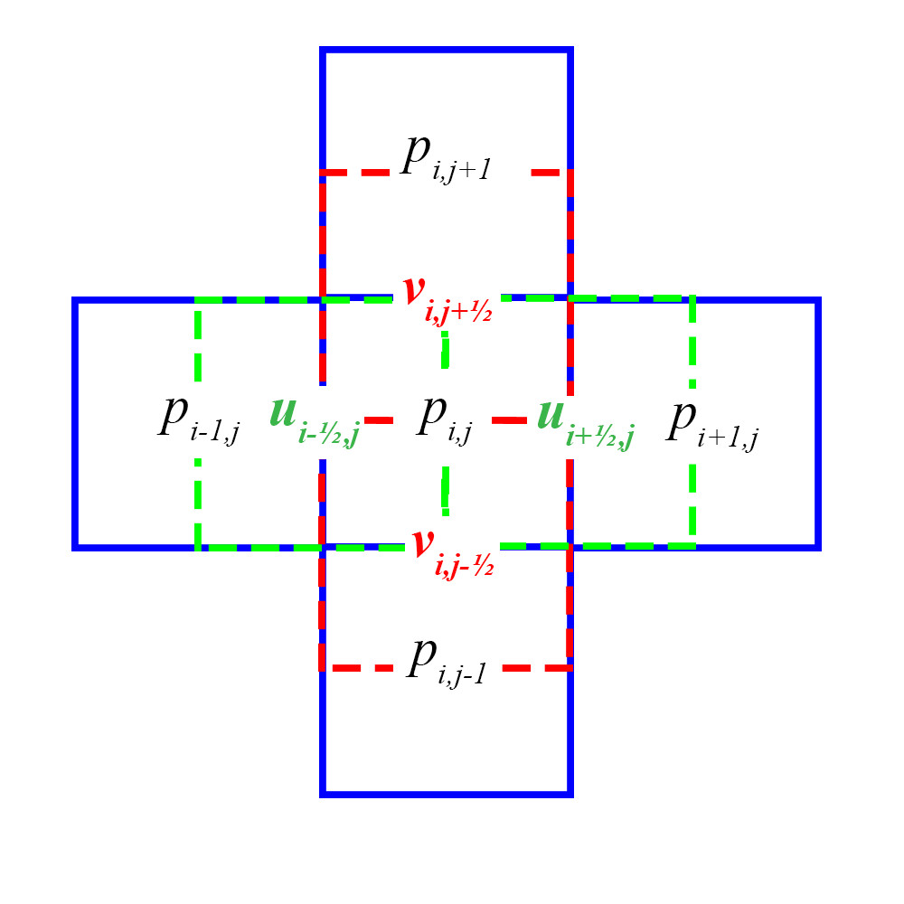
Figure 1: Mesh-staggering for the two dimensional case (left) and for the three-dimensional case (right).

where $s$ stands for $x$, $y$ or $z$. A simplified picture of the resulting mesh-staggering is depicted in Figure 1 for the two dimensional and for the three dimensional case. In our particular implementation, the $\varphi(\xi)$ are defined by the Lagrange interpolation polynomials passing through the Gauss-Legendre quadrature points on the unit interval $[0,1]$, see [59], hence leading to an orthogonal nodal basis. As a result, all element mass matrices are diagonal.

By direct substitution of the definitions (6-9) into (4-5) and by using the same basis functions also as test functions, one obtains the following semi-discrete staggered DG discretiation of the incompressible Navier-Stokes equations:

$$\int\limits_{T_{i+\frac{1}{2},j,k}}\psi_{m_{1}}(x)\omega_{m_{2}}(y)\omega_{m_{3}}(z)\left(\frac{\partial u_{h}}{\partial t}+\nabla\cdot\mathbf{F}_{u}+\partial_{x}p_{h}\right)d\mathbf{x}=0,$$ (10)

$$\int\limits_{T_{i,j+\frac{1}{2},k}}\omega_{m_{1}}(x)\psi_{m_{2}}(y)\omega_{m_{3}}(z)\left(\frac{\partial v_{h}}{\partial t}+\nabla\cdot\mathbf{F}_{v}+\partial_{y}p_{h}\right)d\mathbf{x}=0,$$ (11)

$$\int\limits_{T_{i,j,k+\frac{1}{2}}}\omega_{m_{1}}(x)\omega_{m_{2}}(y)\psi_{m_{3}}(z)\left(\frac{\partial w_{h}}{\partial t}+\nabla\cdot\mathbf{F}_{w}+\partial_{z}p_{h}\right)d\mathbf{x}=0,$$ (12)

$$\int\limits_{T_{i,j,k}}\omega_{m_{1}}(x)\omega_{m_{2}}(y)\omega_{m_{3}}(z)\,\left(\nabla\cdot\mathbf{v}_{h}\right)d\mathbf{x}=0.$$ (13)

Integration of (13) by parts yields

$$\int\limits_{\partial T_{i,j,k}}\omega_{m_{1}}(x)\omega_{m_{2}}(y)\omega_{m_{3}}(z)\,\mathbf{v}_{h}\cdot\vec{n}\,dS-\int\limits_{T_{i,j,k}}\nabla\left(\omega_{m_{1}}(x)\omega_{m_{2}}(y)\omega_{m_{3}}(z)\right)\cdot\mathbf{v}_{h}\,d\mathbf{x}=0,$$ (14)

which is well defined, since the velocity vector $\mathbf{v}_{h}$ is continuous across the element boundary $\partial T_{i,j,k}$, thanks to the use of a staggered grid approach. However, because of the staggering, $p_{h}$ is discontinuous inside the domains of integration of the momentum equations (10-12) and the following jump contributions arise

$$\int\limits_{x_{i}}^{x_{i+1}}\int\limits_{y_{j-\frac{1}{2}}}^{y_{j+\frac{1}{2}}}\int\limits_{z_{k-\frac{1}{2}}}^{z_{k+\frac{1}{2}}}\psi_{m_{1}}(x)\omega_{m_{2}}(y)\omega_{m_{3}}(z)\partial_{x}p_{h}(\mathbf{x},t)\,d\mathbf{x}=$$

$$\int\limits_{x_{i}}^{x_{i+\frac{1}{2}}}\int\limits_{y_{j-\frac{1}{2}}}^{y_{j+\frac{1}{2}}}\int\limits_{z_{k-\frac{1}{2}}}^{z_{k+\frac{1}{2}}}\psi_{m_{1}}(x)\omega_{m_{2}}(y)\omega_{m_{3}}(z)\partial_{x}p_{i,j,k}(\mathbf{x},t)\,d\mathbf{x}+\int\limits_{x_{i+\frac{1}{2}}}^{x_{i+1}}\int\limits_{y_{j-\frac{1}{2}}}^{y_{j+\frac{1}{2}}}\int\limits_{z_{k-\frac{1}{2}}}^{z_{k+\frac{1}{2}}}\psi_{m_{1}}(x)\omega_{m_{2}}(y)\omega_{m_{3}}(z)\partial_{x}p_{i+1,j,k}(\mathbf{x},t)\,d\mathbf{x}+$$

$$+\int\limits_{y_{j-\frac{1}{2}}}^{y_{j+\frac{1}{2}}}\int\limits_{z_{k-\frac{1}{2}}}^{z_{k+\frac{1}{2}}}\psi_{m_{1}}(x_{i+\frac{1}{2}})\omega_{m_{2}}(y)\omega_{m_{3}}(z)\left(p_{i+1,j,k}(x_{i+\frac{1}{2}},y,z,t)-p_{i,j,k}(x_{i+\frac{1}{2}},y,z,t)\right)dydz,$$ (15)

with similar expressions also in the $y$- and $z$-momentum equations, respectively. Thus, an efficient semi-implicit time discretization of the governing PDE system is obtained by introducing an explicit discretization of the nonlinear convective and viscous terms and an implicit discretization of the pressure gradients in the momentum equations (10-12) and of the incompressibility condition (13). After evaluating the integrals and via some manipulations one can obtain the following coupled system of equations for the vectors of the degrees of freedom of velocity $\widehat{\mathbf{U}}^{n+1}_{i+\frac{1}{2},j,k}=\hat{u}^{n+1}_{l,i+\frac{1}{2},j,k}$, $\widehat{\mathbf{V}}^{n+1}_{i,j+\frac{1}{2},k}=\hat{v}^{n+1}_{l,i,j+\frac{1}{2},k}$, $\widehat{\mathbf{W}}^{n+1}_{i,j,k+\frac{1}{2}}=\hat{w}^{n+1}_{l,i,j,k+\frac{1}{2}}$ and pressure $\widehat{\mathbf{P}}^{n+1}_{i,j,k}=\hat{p}^{n+1}_{l,i,j,k}$, respectively:

$$\mathbf{M}^{\textsl{xyz}}\cdot\left(\widehat{\mathbf{U}}^{n+1}_{i+\frac{1}{2},j,k}-\widehat{\mathbf{Fu}}^{n}_{i+\frac{1}{2},j,k}\right)+\frac{\Delta t}{\Delta x}\mathbf{M}^{\textsl{yz}}\cdot\left(\mathbf{R}_{\text{{{v}}}}^{\textsl{x}}\cdot\widehat{\mathbf{P}}^{n+\theta}_{i+1,j,k}-\mathbf{L}_{\text{{{v}}}}^{\textsl{x}}\cdot\widehat{\mathbf{P}}^{n+\theta}_{i,j,k}\right) =0,$$ (16)

$$\mathbf{M}^{\textsl{xyz}}\cdot\left(\widehat{\mathbf{V}}^{n+1}_{i,j+\frac{1}{2},k}-\widehat{\mathbf{Fv}}^{n}_{i,j+\frac{1}{2},k}\right)+\frac{\Delta t}{\Delta y}\mathbf{M}^{\textsl{zx}}\cdot\left(\mathbf{R}_{\text{{{v}}}}^{\textsl{y}}\cdot\widehat{\mathbf{P}}^{n+\theta}_{i,j+1,k}-\mathbf{L}_{\text{{{v}}}}^{\textsl{y}}\cdot\widehat{\mathbf{P}}^{n+\theta}_{i,j,k}\right) =0,$$ (17)

$$\mathbf{M}^{\textsl{xyz}}\cdot\left(\widehat{\mathbf{W}}^{n+1}_{i,j,k+\frac{1}{2}}-\widehat{\mathbf{Fw}}^{n}_{i,j,k+\frac{1}{2}}\right)+\frac{\Delta t}{\Delta z}\mathbf{M}^{\textsl{xy}}\cdot\left(\mathbf{R}_{\text{{{v}}}}^{\textsl{z}}\cdot\widehat{\mathbf{P}}^{n+\theta}_{i,j,k+1}-\mathbf{L}_{\text{{{v}}}}^{\textsl{z}}\cdot\widehat{\mathbf{P}}^{n+\theta}_{i,j,k}\right) =0,$$ (18)

$$\frac{\mathbf{M}^{\textsl{yz}}\left(\mathbf{R}_{\text{{{p}}}}^{\textsl{x}}\cdot\widehat{\mathbf{U}}^{n+1}_{i+\frac{1}{2},j,k}\!-\!\mathbf{L}_{\text{{{p}}}}^{\textsl{x}}\cdot\widehat{\mathbf{U}}^{n+1}_{i-\frac{1}{2},j,k}\right)}{\Delta x}+\frac{\mathbf{M}^{\textsl{zx}}\left(\mathbf{R}_{\text{{{p}}}}^{\textsl{y}}\cdot\widehat{\mathbf{V}}^{n+1}_{i,j+\frac{1}{2},k}\!-\!\mathbf{L}_{\text{{{p}}}}^{\textsl{y}}\cdot\widehat{\mathbf{V}}^{n+1}_{i,j-\frac{1}{2},k}\right)}{\Delta y}+\frac{\mathbf{M}^{\textsl{xy}}\left(\mathbf{R}_{\text{{{p}}}}^{\textsl{z}}\cdot\widehat{\mathbf{W}}^{n+1}_{i,j,k+\frac{1}{2}}\!-\!\mathbf{L}_{\text{{{p}}}}^{\textsl{z}}\cdot\widehat{\mathbf{W}}^{n+1}_{i,j,k-\frac{1}{2}}\right)}{\Delta z}=0.$$ (19)

Here, the following matrices have been used

$$\mathbf{M}^{\textsl{}}\equiv\left\{M_{pq}\right\}_{p,q=0,...,N}\equiv\left\{\int\limits_{0}^{1}\,\varphi_{p}\left(\xi\right)\varphi_{q}\left(\xi\right)d\xi\right\}_{p,q=0,...,N}$$

$$\mathbf{R}_{\text{{{v}}}}^{\textsl{}}\equiv\left\{R_{pq}\right\}_{p,q=0,...,N}\equiv\left\{\varphi_{p}(\frac{1}{2})\varphi_{q}(0)+\frac{1}{2}\int\limits_{0}^{1}\,\varphi_{p}\left(\frac{1}{2}+\frac{\xi}{2}\right)\varphi_{q}^{\prime}\left(\frac{\xi}{2}\right)d\xi\right\}_{p,q=0,...,N}$$

$$\mathbf{L}_{\text{{{v}}}}^{\textsl{}}\equiv\left\{L_{pq}\right\}_{p,q=0,...,N}\equiv\left\{\varphi_{p}(\frac{1}{2})\varphi_{q}(1)-\frac{1}{2}\int\limits_{0}^{1}\,\varphi_{p}\left(\frac{\xi}{2}\right)\varphi_{q}^{\prime}\left(\frac{1}{2}+\frac{\xi}{2}\right)d\xi\right\}_{p,q=0,...,N}$$

$$\mathbf{R}_{\text{{{p}}}}^{\textsl{}}\equiv\left\{L^{T}_{pq}\right\}_{p,q=0,...,N}\equiv\left\{\varphi_{p}(1)\varphi_{q}(\frac{1}{2})-\frac{1}{2}\int\limits_{0}^{1}\,\varphi_{p}^{\prime}\left(\frac{1}{2}+\frac{\xi}{2}\right)\varphi_{q}\left(\frac{\xi}{2}\right)d\xi\right\}_{p,q=0,...,N}$$

$$\mathbf{L}_{\text{{{p}}}}^{\textsl{}}\equiv\left\{R^{T}_{pq}\right\}_{p,q=0,...,N}\equiv\left\{\varphi_{p}(0)\varphi_{q}(\frac{1}{2})+\frac{1}{2}\int\limits_{0}^{1}\,\varphi_{p}^{\prime}\left(\frac{\xi}{2}\right)\varphi_{q}\left(\frac{1}{2}+\frac{\xi}{2}\right)d\xi\right\}_{p,q=0,...,N},$$ (20)

which operate along a generic vector of degrees of freedom $\widehat{\mathbf{X}}=\left\{\hat{x}_{mm^{\prime}m^{\prime\prime}}\right\}_{m,m^{\prime},m^{\prime\prime}=0,..,N},$via the tensor products

$$\mathbf{Z}^{\textsl{x}}\cdot\widehat{\mathbf{X}}=Z_{ml}I_{m^{\prime}l^{\prime}}I_{m^{\prime\prime}l^{\prime\prime}}\hat{x}_{l\,l^{\prime}l^{\prime\prime}},\qquad\mathbf{Z}^{\textsl{y}}\cdot\widehat{\mathbf{X}}=I_{ml}Z_{m^{\prime}l^{\prime}}I_{m^{\prime\prime}l^{\prime\prime}}\hat{x}_{l\,l^{\prime}l^{\prime\prime}},\qquad\mathbf{Z}^{\textsl{z}}\cdot\widehat{\mathbf{X}}=I_{ml}I_{m^{\prime}l^{\prime}}Z_{m^{\prime\prime}l^{\prime\prime}}\hat{x}_{l\,l^{\prime}l^{\prime\prime}}$$ (21)

and

$$\begin{array}[]{rl}\mathbf{Z}^{\textsl{x${}_{i}$ x${}_{j}$}}&\equiv\mathbf{Z}^{\textsl{x${}_{i}$}}\cdot\mathbf{Z}^{\textsl{x${}_{j}$}},\\ \mathbf{Z}^{\textsl{x${}_{i}$ x${}_{j}$ x${}_{k}$}}&\equiv\mathbf{Z}^{\textsl{x${}_{i}$}}\cdot\mathbf{Z}^{\textsl{x${}_{j}$}}\cdot\mathbf{Z}^{\textsl{x${}_{k}$}},\end{array}\;\;\;\text{with}\;x_{i},x_{j},x_{k}\in\left\{x,y,z\right\}$$ (24)

where $\mathbf{Z}$ is a real square matrix, $I$ is the identity operator and the Einstein convention of summation over repeated indexes is assumed. Note that for the pressure gradients an implicitness factor $\theta\in[\frac{1}{2},1]$ has been introduced, by defining $\widehat{\mathbf{P}}^{n+\theta}=\theta\widehat{\mathbf{P}}^{n+1}+\left(1-\theta\right)\widehat{\mathbf{P}}^{n}$. By choosing $\theta=\left.1\middle/2\right.$, the time discretization of (16)-(19) is equivalent to a Crank-Nicolson scheme, which is second-order accurate in time.

$\widehat{\mathbf{Fu}}^{n}$, $\widehat{\mathbf{Fv}}^{n}$ and $\widehat{\mathbf{Fw}}^{n}$ can be computed with any suitable explicit discretization for advection and diffusion. An insight into these terms will be given later in the text.

The coupled system of equations (16)-(19) has a typical saddle point structure that arises naturally from the discretization of the incompressible Navier-Stokes equations. Its direct solution can be cumbersome, since it involves four unknown quantities: three velocity components and the scalar pressure. The complexity of the problem can be considerably reduced with a very simple manipulation. After multiplying the momentum equations by the inverse of the mass matrix $\mathbf{M}^{\textsl{xyz}}$, the discrete velocity equations can be substituted into the discrete incompressibility condition (19). As a result, one obtains one single linear system for the degrees of freedom of the unknown scalar pressure $\widehat{\mathbf{P}}^{n+1}$ only, i.e.

$$\frac{\theta\Delta t}{\Delta x^{2}}\left(\mathbf{M}^{\textsl{yz}}\cdot\mathbb{R}^{\textsl{x}}\right)\cdot\widehat{\mathbf{P}}^{n+1}_{i+1,j,k}+\frac{\theta\Delta t}{\Delta y^{2}}\left(\mathbf{M}^{\textsl{zx}}\cdot\mathbb{R}^{\textsl{y}}\right)\cdot\widehat{\mathbf{P}}^{n+1}_{i,j+1,k}+\frac{\theta\Delta t}{\Delta z^{2}}\left(\mathbf{M}^{\textsl{xy}}\cdot\mathbb{R}^{\textsl{z}}\right)\cdot\widehat{\mathbf{P}}^{n+1}_{i,j,k+1}+$$

$$+\left(\frac{\theta\Delta t}{\Delta x^{2}}\mathbf{M}^{\textsl{yz}}\cdot\mathbb{C}^{\textsl{x}}+\frac{\theta\Delta t}{\Delta y^{2}}\mathbf{M}^{\textsl{zx}}\cdot\mathbb{C}^{\textsl{y}}+\frac{\theta\Delta t}{\Delta z^{2}}\mathbf{M}^{\textsl{xy}}\cdot\mathbb{C}^{\textsl{z}}\right)\cdot\widehat{\mathbf{P}}^{n+1}_{i,j,k}+$$

$$+\frac{\theta\Delta t}{\Delta x^{2}}\left(\mathbf{M}^{\textsl{yz}}\cdot\mathbb{L}^{\textsl{x}}\right)\cdot\widehat{\mathbf{P}}^{n+1}_{i-1,j,k}+\frac{\theta\Delta t}{\Delta y^{2}}\left(\mathbf{M}^{\textsl{zx}}\cdot\mathbb{L}^{\textsl{y}}\right)\cdot\widehat{\mathbf{P}}^{n+1}_{i,j-1,k}+\frac{\theta\Delta t}{\Delta z^{2}}\left(\mathbf{M}^{\textsl{xy}}\cdot\mathbb{L}^{\textsl{z}}\right)\cdot\widehat{\mathbf{P}}^{n+1}_{i,j,k-1} =\widehat{\mathbf{b}}^{n}_{i,j,k},$$ (25)

$$\text{for}\;\;\;i=2,...,N_{x}-1;\;\;\;j=2,...,N_{y}-1;\;\;\,k=2,...,N_{z}-1$$

Here, the following new tensors have been defined

$$\mathbb{R}^{\textsl{}}=-\left(\mathbf{R}_{\text{{{p}}}}^{\textsl{}}\cdot\mathbf{M}^{\mathbf{-1}\,\textsl{}}\cdot\mathbf{R}_{\text{{{v}}}}^{\textsl{}}\right),\;\;\;\mathbb{L}^{\textsl{}}=-\left(\mathbf{L}_{\text{{{p}}}}^{\textsl{}}\cdot\mathbf{M}^{\mathbf{-1}\,\textsl{}}\cdot\mathbf{L}_{\text{{{v}}}}^{\textsl{}}\right),\;\;\;\mathbb{C}^{\textsl{}}=+\left(\mathbf{R}_{\text{{{p}}}}^{\textsl{}}\cdot\mathbf{M}^{\mathbf{-1}\,\textsl{}}\cdot\mathbf{L}_{\text{{{v}}}}^{\textsl{}}\right)+\left(\mathbf{L}_{\text{{{p}}}}^{\textsl{}}\cdot\mathbf{M}^{\mathbf{-1}\,\textsl{}}\cdot\mathbf{R}_{\text{{{v}}}}^{\textsl{}}\right).$$ (26)

System (25) can be written in compact form as $\mathbb{H}\cdot\mathpzc{P}^{n+1}=\mathpzc{b}^{n}$, where $\mathbb{H}$ is the block coefficient matrix, $\mathpzc{P}^{n+1}$ collects all the unknown pressure degrees of freedom of the computational domain at the new time level and $\mathpzc{b}^{n}$ collects all the known terms of the equations. All the real advantages of the chosen mesh-staggering and the semi-implicit discretization arise in the particular features of the resulting linear system (25). The substitution of the discrete velocity equation into the discrete divergence condition can be seen as the application of the Schur complement to the saddle point problem (16)-(19). The particular grid staggering used in this paper, i.e. the so-called C-grid according to the nomenclature of Arakawa & Lamb [2], has been selected to be the one that minimizes the stencil size of the resulting pressure system. In fact, $\mathbb{H}$ is only block hepta-diagonal for the three dimensional case, and only block penta-diagonal for the two dimensional case. Table 4 shows the stencil-sizes (number of non-zero blocks) of the resulting algebraic systems for the pressure, varying for different choices of the grid type and for different numbers of space dimensions. In particular, the symmetry of $\mathbb{H}$ can be easily proven by showing directly from the definition in eq. (25) that $\mathbb{H}=\mathbb{H}^{T}$. The key point of the demonstration is that the next three equivalences are true by construction of (20)

$$\mathbf{M}^{\textsl{T}} =\mathbf{M}^{\textsl{}}$$

$$\mathbb{R}^{\textsl{T}} =-\left(\mathbf{R}_{\text{{{p}}}}^{\textsl{}}\cdot\mathbf{M}^{\mathbf{-1}\,\textsl{}}\cdot\mathbf{R}_{\text{{{v}}}}^{\textsl{}}\right)^{T}=-\left(\mathbf{R}_{\text{{{v}}}}^{\textsl{T}}\cdot\left(\mathbf{M}^{\mathbf{-1}\,\textsl{}}\right)^{T}\cdot\mathbf{R}_{\text{{{p}}}}^{\textsl{T}}\right)=-\left(\mathbf{L}_{\text{{{p}}}}^{\textsl{}}\cdot\mathbf{M}^{\mathbf{-1}\,\textsl{}}\cdot\mathbf{L}_{\text{{{v}}}}^{\textsl{}}\right)\equiv\mathbb{L}^{\textsl{}},$$

$$\mathbb{C}^{\textsl{T}} =\left(\mathbf{R}_{\text{{{p}}}}^{\textsl{}}\cdot\mathbf{M}^{\mathbf{-1}\,\textsl{}}\cdot\mathbf{L}_{\text{{{v}}}}^{\textsl{}}\right)^{T}+\left(\mathbf{L}_{\text{{{p}}}}^{\textsl{}}\cdot\mathbf{M}^{\mathbf{-1}\,\textsl{}}\cdot\mathbf{R}_{\text{{{v}}}}^{\textsl{}}\right)^{T}=$$

$$=\left(\mathbf{L}_{\text{{{v}}}}^{\textsl{T}}\cdot\left(\mathbf{M}^{\mathbf{-1}\,\textsl{}}\right)^{T}\cdot\mathbf{R}_{\text{{{p}}}}^{\textsl{T}}\right)+\left(\mathbf{R}_{\text{{{v}}}}^{\textsl{T}}\cdot\left(\mathbf{M}^{\mathbf{-1}\,\textsl{}}\right)^{T}\cdot\mathbf{L}_{\text{{{p}}}}^{\textsl{T}}\right)=$$

$$=\left(\mathbf{R}_{\text{{{p}}}}^{\textsl{}}\cdot\mathbf{M}^{\mathbf{-1}\,\textsl{}}\cdot\mathbf{L}_{\text{{{v}}}}^{\textsl{}}\right)+\left(\mathbf{L}_{\text{{{p}}}}^{\textsl{}}\cdot\mathbf{M}^{\mathbf{-1}\,\textsl{}}\cdot\mathbf{R}_{\text{{{v}}}}^{\textsl{}}\right)\equiv\mathbb{C}^{\textsl{}}.$$ (27)

Further to that, it can be shown that $\mathbb{H}$ is also positive semi-definite in the general case, i.e.

$$\mathpzc{v}^{T}\mathbb{H}\mathpzc{v}\geq 0,\qquad\forall\mathpzc{v}\neq 0.$$ (28)

Note that in this notation, equation (25) can be written as $\mathbb{H}^{i,j,k}\cdot\mathpzc{P}^{n+1}=\mathpzc{b}^{n}_{i,j,k}$. Matrix $\mathbb{H}$ can be written in the form of a tensor product of the matrices $\mathbb{H}=\mathbb{H}^{xyz}=\mathbb{H}^{x}\mathbb{H}^{y}\mathbb{H}^{z}$. Next, the positive semi-definiteness is shown to be valid for the one-dimensional case $\mathbb{H}=\mathbb{H}^{x}$, then the extension to $\mathbb{H}=\mathbb{H}^{xyz}$ is straightforward. If $d=1$ and periodic boundary conditions are assumed the left hand side of (25) can be written as

$$\mathbb{H}^{i}\cdot\mathpzc{P}^{n+1}= -\left[\left(\mathbf{R}_{\text{{{p}}}}^{\textsl{}}\cdot\mathbf{M}^{\mathbf{-1}\,\textsl{}}\cdot\mathbf{R}_{\text{{{v}}}}^{\textsl{}}\right)\cdot\widehat{\mathbf{P}}^{n+1}_{i+1}-\left(\mathbf{R}_{\text{{{p}}}}^{\textsl{}}\cdot\mathbf{M}^{\mathbf{-1}\,\textsl{}}\cdot\mathbf{L}_{\text{{{v}}}}^{\textsl{}}\right)\widehat{\mathbf{P}}^{n+1}_{i}\right]+$$

$$+\left[\left(\mathbf{L}_{\text{{{p}}}}^{\textsl{}}\cdot\mathbf{M}^{\mathbf{-1}\,\textsl{}}\cdot\mathbf{R}_{\text{{{v}}}}^{\textsl{}}\right)\widehat{\mathbf{P}}^{n+1}_{i}-\left(\mathbf{L}_{\text{{{p}}}}^{\textsl{}}\cdot\mathbf{M}^{\mathbf{-1}\,\textsl{}}\cdot\mathbf{L}_{\text{{{v}}}}^{\textsl{}}\right)\widehat{\mathbf{P}}^{n+1}_{i-1}\right],$$ (29)

$$\text{for}\;\;\;i=1,...,N_{x},\;\;\;\text{with}\;P_{N_{x}+1}=P_{1};$$

where the mass matrix tensors and the discretization constants can be removed after multiplication with suitable factors from the left. Now a new nomenclature is introduced to emphasize the features of the system,

$$\mathcal{R}=\mathbf{R}_{\text{{{v}}}}^{\textsl{}}\equiv\mathbf{L}_{\text{{{p}}}}^{\textsl{T}},\;\;\;\mathcal{L}=\mathbf{L}_{\text{{{v}}}}^{\textsl{}}\equiv\mathbf{R}_{\text{{{p}}}}^{\textsl{T}},$$ (30)

from the definitions (20). Now, relation (29) can be written as

$$\mathbb{H}^{i}\cdot\mathpzc{P}^{n+1}= -\left[\mathcal{L}^{T}\mathbf{M}^{-1}\mathcal{R}\cdot\widehat{\mathbf{P}}^{n+1}_{i+1}-\mathcal{L}^{T}\mathbf{M}^{-1}\mathcal{L}\cdot\widehat{\mathbf{P}}^{n+1}_{i}\right]+\left[\mathcal{R}^{T}\mathbf{M}^{-1}\mathcal{R}\cdot\widehat{\mathbf{P}}^{n+1}_{i}-\mathcal{R}^{T}\mathbf{M}^{-1}\mathcal{L}\cdot\widehat{\mathbf{P}}^{n+1}_{i-1}\right],$$

$$\text{for}\;\;\;i=1,...,N_{x},\;\;\;\text{with}\;P_{N_{x}+1}=P_{1};$$

Then, the global system can be written as

$$\mathbb{H}\cdot\mathpzc{P}^{n+1} \equiv\left(\begin{array}[]{ccccc}-\mathcal{L}^{T}&0&\cdots&0&\mathcal{R}^{T}\\ \mathcal{R}^{T}&-\mathcal{L}^{T}&0&0&0\\ 0&\mathcal{R}^{T}&-\mathcal{L}^{T}&\ddots&\vdots\\ \vdots&0&\ddots&\ddots&0\\ 0&\cdots&0&\mathcal{R}^{T}&-\mathcal{L}^{T}\end{array}\right)\cdot\mathbb{M}^{-1}\cdot\left(\begin{array}[]{ccccc}-\mathcal{L}&\mathcal{R}&0&\cdots&0\\ 0&-\mathcal{L}&\mathcal{R}&0&0\\ \vdots&0&-\mathcal{L}&\ddots&0\\ 0&0&\ddots&\ddots&\mathcal{R}\\ \mathcal{R}&0&\cdots&0&-\mathcal{L}\end{array}\right)\cdot\left(\begin{array}[]{c}\widehat{\mathbf{P}}^{n+1}_{1}\\ \widehat{\mathbf{P}}^{n+1}_{2}\\ \vdots\\ \widehat{\mathbf{P}}^{n+1}_{N_{x}-1}\\ \widehat{\mathbf{P}}^{n+1}_{N_{x}}\end{array}\right)=\mathpzc{b}^{n},$$ (46)

where the diagonal mass matrix $\mathbb{M}$ has been introduced. Matrix $\mathbb{H}$ is proved to be positive semi-definite because it can be decomposed into the matrix product

$$\mathpzc{v}^{T}\mathbb{H}\mathpzc{v}\equiv\mathpzc{v}^{T}\mathcal{D}^{T}\mathbb{M}^{-1}\mathcal{D}\mathpzc{v}=\mathpzc{w}^{T}\mathbb{M}^{-1}\mathpzc{w}\geq 0,\;\;\;\text{with}\;\;\;\mathpzc{w}=\mathcal{D}\mathpzc{v}\qquad\forall\;\mathpzc{v}$$

because the mass matrix is positive definite. Notice that

$$\mathcal{D}=\left(\begin{array}[]{ccccc}-\mathcal{L}&\mathcal{R}&0&\cdots&0\\ 0&-\mathcal{L}&\mathcal{R}&0&0\\ \vdots&0&-\mathcal{L}&\ddots&0\\ 0&0&\ddots&\ddots&\mathcal{R}\\ \mathcal{R}&0&\cdots&0&-\mathcal{L}\end{array}\right)$$ (52)

is precisely the weak form of the gradient operator, in fact

$$\partial_{x}p\xrightarrow{\;\;\;\int_{d\Omega^{*}}\psi\cdot\;\;\;}\mathcal{D}^{i}\,\mathpzc{P}=\mathcal{R}\cdot\widehat{\mathbf{P}}_{i+1}-\mathcal{L}\cdot\widehat{\mathbf{P}}_{i}$$ (53)

This is an interesting property because the problem of the uniqueness of the solutions of the pressure system is shifted to the uniqueness of the solutions of

$$\mathcal{D}\,\mathpzc{P}=\text{right hand side}.$$ (54)

that in ensured in general up to the solutions of $\mathcal{D}\,\mathpzc{P}=0$. This means that (for periodic boundaries) the discrete pressure $\mathpzc{P}$ is defined up to weak solutions of $\partial_{x}p=0$, which is exactly what one could expect from a discrete formulation of the incompressible Navier-Stokes equations. If pressure boundary conditions are specified, it can be verified easily that the resulting system for the pressure is indeed symmetric and positive-definite. We further observe all in our numerical experiments that the pressure system seems to be reasonably well conditioned, since the conjugate gradient method converges in rather few iterations even without the use of any preconditioner. This is a rather unique feature among existing implicit DG schemes.

Future research is concerned with the theoretical analysis of the condition number of the resulting linear systems of our method and the design of specific preconditioners for Krylov subspace solvers, using the theory of matrix-valued symbols and Generalized Locally Toeplitz (GLT) algebras, see [121, 77, 122, 134].

Finally, once the pressure $\mathpzc{P}^{n+1}$ has been computed, the velocities can be updated directly accordingly to equations (16-18).

2.2 Explicit discretization of the nonlinear convective and viscous terms

For an explicit discretization of the nonlinear convective and viscous terms, a standard DG scheme based on the Rusanov flux (local Lax-Friedrichs flux [118, 130]) can be adopted on the main grid, see also [72, 57, 83] for numerical flux functions in the presence of physical viscosity:

$$\widehat{\mathbf{Fu}}^{n}_{i,j,k} =\widehat{\mathbf{U}}^{n}_{i,j,k}-\frac{\Delta t}{\Delta x\Delta y\Delta z}\left(\mathbf{M}^{\textsl{xyz}}\right)^{-1}\cdot\left(\,\int\limits_{\partial T_{i,j,k}}\bm{\omega}\mathbf{F}_{u}\cdot\vec{n}dS-\int\limits_{T_{i,j,k}}\nabla\bm{\omega}\cdot\mathbf{F}_{u}\,d\mathbf{x}\right)$$ (55)

$$\widehat{\mathbf{Fv}}^{n}_{i,j,k} =\widehat{\mathbf{V}}^{n}_{i,j,k}-\frac{\Delta t}{\Delta x\Delta y\Delta z}\left(\mathbf{M}^{\textsl{xyz}}\right)^{-1}\cdot\left(\,\int\limits_{\partial T_{i,j,k}}\bm{\omega}\mathbf{F}_{v}\cdot\vec{n}dS-\int\limits_{T_{i,j,k}}\nabla\bm{\omega}\cdot\mathbf{F}_{v}\,d\mathbf{x}\right)$$ (56)

$$\widehat{\mathbf{Fw}}^{n}_{i,j,k} =\widehat{\mathbf{W}}^{n}_{i,j,k}-\frac{\Delta t}{\Delta x\Delta y\Delta z}\left(\mathbf{M}^{\textsl{xyz}}\right)^{-1}\cdot\left(\,\int\limits_{\partial T_{i,j,k}}\bm{\omega}\mathbf{F}_{w}\cdot\vec{n}dS-\int\limits_{T_{i,j,k}}\nabla\bm{\omega}\cdot\mathbf{F}_{w}\,d\mathbf{x}\right),$$ (57)

where the numerical flux has the following simple form

$$\mathbf{F}_{q}\cdot\vec{n} =\frac{1}{2}\left(\mathbf{F}^{+}_{q}+\mathbf{F}^{-}_{q}\right)\cdot\vec{n}-\frac{1}{2}s_{q}\left(q^{+}-q^{-}\right)\;\;\;\text{with}\;q=u,v,w.$$ (58)

where $s_{q}$ are the maximum eigenvalues of the Jacobian of the convective and viscous flux tensor

$$s_{q} =2\,\text{max}\left(|q^{+}|,|q^{-}|\right)+2\nu\frac{2N+1}{\Delta x_{q}\sqrt{\left.{\pi}\middle/{2}\right.}}\;\;\;\;\;\;\text{with}\;(q,\Delta x_{q})=(u,\Delta x),(v,\Delta y),(w,\Delta z).$$ (59)

A linear transformation that allows to compute (55-57) with the velocity polynomials centered in the main grid is the $L_{2}$-projection

$$\widehat{\mathbf{U}}^{n}_{i,j,k} =\left(\mathbf{M}^{\textsl{x}}\right)^{-1}\cdot\left(\mathbf{M}^{Lx}\cdot\widehat{\mathbf{U}}^{n}_{i-\frac{1}{2},j,k}+\mathbf{M}^{Rx}\cdot\widehat{\mathbf{U}}^{n}_{i+\frac{1}{2},j,k}\right),$$ (60)

$$\widehat{\mathbf{V}}^{n}_{i,j,k} =\left(\mathbf{M}^{\textsl{y}}\right)^{-1}\cdot\left(\mathbf{M}^{Ly}\cdot\widehat{\mathbf{V}}^{n}_{i,j-\frac{1}{2},k}+\mathbf{M}^{Ry}\cdot\widehat{\mathbf{V}}^{n}_{i,j+\frac{1}{2},k}\right),$$ (61)

$$\widehat{\mathbf{W}}^{n}_{i,j,k} =\left(\mathbf{M}^{\textsl{z}}\right)^{-1}\cdot\left(\mathbf{M}^{Lz}\cdot\widehat{\mathbf{W}}^{n}_{i,j,k-\frac{1}{2}}+\mathbf{M}^{Rz}\cdot\widehat{\mathbf{W}}^{n}_{i,j,k+\frac{1}{2}}\right),$$ (62)

with

$$\mathbf{M}^{L}=\left\{M^{L}_{pq}\right\}_{p,q=0,..,N}=\left\{\frac{1}{2}\int\limits_{0}^{1}\varphi_{p}\left(\frac{\xi}{2}\right)\varphi_{q}\left(\frac{1}{2}+\frac{\xi}{2}\right)\,d\xi\right\}_{p,q=0,..,N}$$

$$\mathbf{M}^{R}=\left\{M^{R}_{pq}\right\}_{p,q=0,..,N}=\left\{\frac{1}{2}\int\limits_{0}^{1}\varphi_{p}\left(\frac{1}{2}+\frac{\xi}{2}\right)\varphi_{q}\left(\frac{\xi}{2}\right)\,d\xi\right\}_{p,q=0,..,N}$$

Once the advection-diffusion terms have been computed on the main grid, they are projected back to the dual grid with

$$\widehat{\mathbf{Fu}}^{n}_{i+\frac{1}{2},j,k} =\left(\mathbf{M}^{\textsl{x}}\right)^{-1}\cdot\left(\mathbf{M}^{Lx}\cdot\widehat{\mathbf{Fu}}^{n}_{i,j,k}+\mathbf{M}^{Rx}\cdot\widehat{\mathbf{Fu}}^{n}_{i+1,j,k}\right),$$ (63)

$$\widehat{\mathbf{Fv}}^{n}_{i,j+\frac{1}{2},k} =\left(\mathbf{M}^{\textsl{y}}\right)^{-1}\cdot\left(\mathbf{M}^{Ly}\cdot\widehat{\mathbf{Fv}}^{n}_{i,j,k}+\mathbf{M}^{Ry}\cdot\widehat{\mathbf{Fv}}^{n}_{i,j+1,k}\right),$$ (64)

$$\widehat{\mathbf{Fw}}^{n}_{i,j,k+\frac{1}{2}} =\left(\mathbf{M}^{\textsl{z}}\right)^{-1}\cdot\left(\mathbf{M}^{Lz}\cdot\widehat{\mathbf{Fw}}^{n}_{i,j,k}+\mathbf{M}^{Rz}\cdot\widehat{\mathbf{Fw}}^{n}_{i,j,k+1}\right).$$ (65)

Since a simple first order Euler time discretization is likely to become linearly unstable, a classical third order TVD Runge-Kutta scheme is used [52, 59, 123, 125, 126, 127]. The explicit discretization has to satisfy a CFL-type time step restriction

$$\Delta t=\text{CFL}\left[\left(2N+1\right)\left(\frac{|u_{\text{max}}|}{\Delta x}+\frac{|v_{\text{max}}|}{\Delta y}+\frac{|w_{\text{max}}|}{\Delta z}\right)+\left(2N+1\right)^{2}\left(\frac{2\nu}{\Delta x^{2}}+\frac{2\nu}{\Delta y^{2}}+\frac{2\nu}{\Delta z^{2}}\right)\right]^{-1},$$ (66)

with $0<$CFL$<1$.

2.3 Implicit diffusion

The discrete formulation of advection and diffusion (55-57) is an explicit discretization of the equation

$$\frac{\partial\mathbf{v}}{\partial t}+\nabla\cdot\mathbf{F}=0.$$ (67)

The time-step restriction (66) can become rather severe, in particular for highly refined meshes and large values of the kinematic viscosity. An important improvement that allows the time-step restriction to become independent of the kinematic viscosity is achieved by taking advantage from an implicit discretization of the viscous terms. In the following, a novel semi-implicit numerical method for the advection-diffusion problem is described. An efficient semi-implicit discretization of equation (67) is obtained by considering the velocity polynomials to be centered in the main grid, and the velocity gradient (i.e. the stress tensor $\nu\nabla\mathbf{v}$) to be defined on the edge-based dual grid. The use of the staggered control volumes for the stress tensor leads to a continuous function $\mathbf{F}_{d}$ across the cell interfaces of the main grid. Hence, integration over the control volume $T_{i,j,k}$ yields

$$\int\limits_{T_{i,j,k}}\omega_{k_{1}}(x)\omega_{k_{2}}(y)\omega_{k_{3}}(z)\left(\nabla\cdot\mathbf{F}_{d}\right)d\mathbf{x}=\int\limits_{\partial T_{i,j,k}}\omega_{k_{1}}(x)\omega_{k_{2}}(y)\omega_{k_{3}}(z)\mathbf{F}_{d}\cdot\vec{n}-\int\limits_{T_{i,j,k}}\nabla\left(\omega_{k_{1}}(x)\omega_{k_{2}}(y)\omega_{k_{3}}(z)\right)\cdot\mathbf{F}_{d}d\mathbf{x},$$ (68)

and then

$$\mathbf{M}^{\textsl{xyz}}\cdot\left(\widehat{\mathbf{U}}^{n+\frac{1}{2}}_{i,j,k}-\widehat{\mathbf{Fu}}^{n}_{i,j,k}\right)-\nu\frac{\Delta t}{\Delta x}\mathbf{M}^{\textsl{yz}}\cdot\left(\mathbf{R}_{\text{{{p}}}}^{\textsl{x}}\cdot\widehat{\mathbf{U}}^{\textsl{(x)}}_{i+\frac{1}{2},j,k}-\mathbf{L}_{\text{{{p}}}}^{\textsl{x}}\cdot\widehat{\mathbf{U}}^{\textsl{(x)}}_{i-\frac{1}{2},j,k}\right)+$$

$$-\nu\frac{\Delta t}{\Delta y}\mathbf{M}^{\textsl{zx}}\cdot\left(\mathbf{R}_{\text{{{p}}}}^{\textsl{y}}\cdot\widehat{\mathbf{U}}^{\textsl{(y)}}_{i,j+\frac{1}{2},k}-\mathbf{L}_{\text{{{p}}}}^{\textsl{y}}\cdot\widehat{\mathbf{U}}^{\textsl{(y)}}_{i,j-\frac{1}{2},k}\right)-\nu\frac{\Delta t}{\Delta z}\mathbf{M}^{\textsl{xy}}\cdot\left(\mathbf{R}_{\text{{{p}}}}^{\textsl{z}}\cdot\widehat{\mathbf{U}}^{\textsl{(z)}}_{i,j,k+\frac{1}{2}}-\mathbf{L}_{\text{{{p}}}}^{\textsl{z}}\cdot\widehat{\mathbf{U}}^{\textsl{(z)}}_{i,j,k-\frac{1}{2}}\right)=0,$$ (69)

where the velocity derivatives can be computed with

$$\widehat{\mathbf{U}}^{\textsl{(x)}}_{i+\frac{1}{2},j,k}=\frac{1}{\Delta x}\left(\mathbf{M}^{\textsl{x}}\right)^{-1}\cdot\left(\mathbf{R}_{\text{{{v}}}}^{\textsl{x}}\cdot\widehat{\mathbf{U}}^{n+\frac{1}{2}}_{i+1,j,k}-\mathbf{L}_{\text{{{v}}}}^{\textsl{x}}\cdot\widehat{\mathbf{U}}^{n+\frac{1}{2}}_{i,j,k}\right),$$ (70)

$$\widehat{\mathbf{U}}^{\textsl{(y)}}_{i,j+\frac{1}{2},k}=\frac{1}{\Delta y}\left(\mathbf{M}^{\textsl{y}}\right)^{-1}\cdot\left(\mathbf{R}_{\text{{{v}}}}^{\textsl{y}}\cdot\widehat{\mathbf{U}}^{n+\frac{1}{2}}_{i+1,j,k}-\mathbf{L}_{\text{{{v}}}}^{\textsl{y}}\cdot\widehat{\mathbf{U}}^{n+\frac{1}{2}}_{i,j,k}\right),$$ (71)

$$\widehat{\mathbf{U}}^{\textsl{(z)}}_{i,j,k+\frac{1}{2}}=\frac{1}{\Delta z}\left(\mathbf{M}^{\textsl{z}}\right)^{-1}\cdot\left(\mathbf{R}_{\text{{{v}}}}^{\textsl{z}}\cdot\widehat{\mathbf{U}}^{n+\frac{1}{2}}_{i+1,j,k}-\mathbf{L}_{\text{{{v}}}}^{\textsl{z}}\cdot\widehat{\mathbf{U}}^{n+\frac{1}{2}}_{i,j,k}\right),$$ (72)

and analogous equations for $\widehat{\mathbf{V}}^{n+\frac{1}{2}}$ and $\widehat{\mathbf{W}}^{n+\frac{1}{2}}$. By a formal substitution of equations (70-72) into (69), the following systems for the velocity components can be written in a very compact form as

$$\left(\mathbb{M}+\nu\mathbb{H}\right)\cdot\mathpzc{U}^{n+\frac{1}{2}}=\mathbb{M}\cdot\mathpzc{Fu}^{n},\;\;\;\left(\mathbb{M}+\nu\mathbb{H}\right)\cdot\mathpzc{V}^{n+\frac{1}{2}}=\mathbb{M}\cdot\mathpzc{Fv}^{n},\;\;\;\left(\mathbb{M}+\nu\mathbb{H}\right)\cdot\mathpzc{W}^{n+\frac{1}{2}}=\mathbb{M}\cdot\mathpzc{Fw}^{n},$$ (73)

by means of the piecewise polynomials $\mathpzc{U}^{n+\frac{1}{2}}$, $\mathpzc{V}^{n+\frac{1}{2}}$, $\mathpzc{W}^{n+\frac{1}{2}}$ on the main grid. Here, $\mathbb{M}>0$ is the diagonal tensor of the element mass matrices, $\mathbb{H}\geq 0$ is exactly the same operator that has been obtained for the pressure system in (29). Then, the tensor coefficient matrices of systems (73) are all positive definite because the sum of a positive semi-definite matrix and a positive definite matrix is positive definite. The right hand sides of the system of equations (73) contains only the fully explicit discretization of the nonlinear convective terms $\mathpzc{Fu}^{n}=\left\{\widehat{\mathbf{Fu}}^{n}\right\}$, $\mathpzc{Fv}^{n}=\left\{\widehat{\mathbf{Fv}}^{n}\right\}$ and $\mathpzc{Fw}^{n}=\left\{\widehat{\mathbf{Fw}}^{n}\right\}$ multiplied by the mass matrix. This means that the CFL-type restriction on the time-step (66) looses the dependency on the viscosity and relaxes to

$$\Delta t=\frac{\text{CFL}}{\left(2N+1\right)}\left(\frac{|u_{\text{max}}|}{\Delta x}+\frac{|v_{\text{max}}|}{\Delta y}+\frac{|w_{\text{max}}|}{\Delta z}\right)^{-1}.$$ (74)

If the solutions of the semi-implicit formulation of the advection-diffusion system (73) substitute the fully explicit terms $\widehat{\mathbf{Fu}}^{n}$, $\widehat{\mathbf{Fv}}^{n}$ and $\widehat{\mathbf{Fw}}^{n}$ in (55-57), a coherent DG scheme is obtained by means of a fractional time-stepping approach. The resulting numerical scheme can be finally written in compact form as

$$\left(\mathbb{M}+\nu\mathbb{H}\right)\cdot\mathpzc{U}^{n+\frac{1}{2}}_{\#}=\mathbb{M}\cdot\mathpzc{Fu}^{n}_{\#},$$ (75)

$$\left(\mathbb{M}+\nu\mathbb{H}\right)\cdot\mathpzc{V}^{n+\frac{1}{2}}_{\#}=\mathbb{M}\cdot\mathpzc{Fv}^{n}_{\#},$$ (76)

$$\left(\mathbb{M}+\nu\mathbb{H}\right)\cdot\mathpzc{W}^{n+\frac{1}{2}}_{\#}=\mathbb{M}\cdot\mathpzc{Fw}^{n}_{\#},$$ (77)

$$\mathbb{H}\cdot\mathpzc{P}^{n+\theta}_{\#}=\mathpzc{b}^{n+\frac{1}{2}}_{\#},$$ (78)

$$\text{with}\;\;\;\mathpzc{b}^{n+\frac{1}{2}}_{\#}\equiv\mathbb{M}^{yz}\left(\mathcal{D}^{x}\right)^{T}\cdot\mathpzc{U}^{n+\frac{1}{2}}_{*}+\mathbb{M}^{zx}\left(\mathcal{D}^{y}\right)^{T}\cdot\mathpzc{V}^{n+\frac{1}{2}}_{*}+\mathbb{M}^{xy}\left(\mathcal{D}^{z}\right)^{T}\cdot\mathpzc{W}^{n+\frac{1}{2}}_{*},$$

$$\mathpzc{U}^{n+1}_{*} =\mathpzc{U}^{n+\frac{1}{2}}_{*}-\frac{\Delta t}{\Delta x}\left(\mathbb{M}^{-1}\mathcal{D}\right)^{x}\cdot\mathpzc{P}^{n+\theta}_{{\#}},$$ (79)

$$\mathpzc{V}^{n+1}_{*} =\mathpzc{V}^{n+\frac{1}{2}}_{*}-\frac{\Delta t}{\Delta y}\left(\mathbb{M}^{-1}\mathcal{D}\right)^{y}\cdot\mathpzc{P}^{n+\theta}_{{\#}},$$ (80)

$$\mathpzc{W}^{n+1}_{*} =\mathpzc{W}^{n+\frac{1}{2}}_{*}-\frac{\Delta t}{\Delta z}\left(\mathbb{M}^{-1}\mathcal{D}\right)^{z}\cdot\mathpzc{P}^{n+\theta}_{{\#}},$$ (81)

where $\mathpzc{Fu}^{n}=\left\{\widehat{\mathbf{Fu}}^{n}\right\}$, $\mathpzc{Fv}^{n}=\left\{\widehat{\mathbf{Fv}}^{n}\right\}$ and $\mathpzc{Fw}^{n}=\left\{\widehat{\mathbf{Fw}}^{n}\right\}$ are the purely explicit discretization of the nonlinear convective terms outlined in the previous section; ’$*$’ is used for the field variables defined along the dual grids; ’$\#$’ for those variables defined along the main grid; notice that the projection of a field variable from the dual grid to the main grid ($\pi_{:*\rightarrow\#}$) and vice versa ($\pi_{:\#\rightarrow*}$) is simply performed by the $L_{2}$ projections defined in (62) and (65), respectively. Once the nonlinear convective terms have been computed with respect to the field variables of the old time step $t^{n}$, then the viscous terms are computed implicitly at a fictitious fractional time-step $t^{n+\frac{1}{2}}$ (75-77). Finally the pressure forces and the incompressibility condition are solved implicitly (78) and the field variables at the future time $t^{n+1}$ are worked out (79-81). The fractional time discretization $t^{n+\frac{1}{2}}$ is only an auxiliary notation emphasizing that it is a intermediate stage. In fact, the real time evolution of the discrete diffusion equations (75-77) is from $t^{n}$ to $t^{n+1}=t^{n}+\Delta t$.

2.4 Numerical validation

In order to check the ability of the new method in solving the governing equations accurately, some different numerical test problems in two and three space dimensions have been chosen, for which an analytical or other numerical reference solutions exist.

2.4.1 Blasius boundary layer

In this test, a steady laminar boundary layer over a flat plate is considered. According to the theory of Prandtl [114, 120], convective terms are of the order $1$ in the boundary layer along the horizontal direction, whereas the vertical accelerations are of the order of the boundary layer thickness. The spatial domain under consideration is $\Omega=[-1,1]\times[0,0.25]$ and the chosen kinematic viscosity is $\nu=10^{-3}$. The flat-plate boundary is imposed at $y=0$ for $x>0$. Constant velocity $\mathbf{v}=(1,0)$ is imposed at the left inflow boundary, constant pressure $p=0$ at the right outflow, no-slip boundary conditions along the wall and no-jump condition in the rest. Results are shown in Fig. 2, obtained with our SIDG-$\textnormal{P}_{7}$ method using $\theta=1$ and a very coarse grid of only $18\times 6$ elements. A very good agreement between the numerical solution obtained with the semi-implicit spectral DG scheme and the Blasius reference solution can be observed. Notice that the complete boundary layer is well resolved inside a single element close to $x=0$.

2.4.2 Lid-driven cavity: 2D

An interesting standard benchmark problem for numerical methods applied to the incompressible Navier-Stokes equations is the lid-driven cavity, see [75]. In this test, a closed square cavity is filled with an incompressible fluid and the flow is driven by the upper wall that moves with velocity $\mathbf{v}=(1,0)$. The main difficulties in solving this problem arise from the singularities of the velocity gradient at the top right and at the top left corners, where the horizontal velocity component is a double valued function: $u=0$ at the left (or right) wall boundary and $u=1$ at the upper moving boundary. Moreover, the pressure is determined only up to a constant, because there are only velocity boundary conditions. The physical domain is $\Omega=[-0.5,0.5]\times[-0.5,0.5]$, the initial condition for velocity and pressure is set to $\mathbf{v}=(0,0)$ and $p=0$. Fig. 3 shows the computed results compared with the reference solution of Ghia et al. [75] next to the two-dimensional view of the velocity magnitude at different Reynolds numbers from Re=$100$ to Re=$3200$, obtained with the $\textnormal{P}_{6}$ version of our staggered semi-implicit spectral DG scheme. The implicitness factor has been chosen equal to $\theta=1$, since only a steady solution is sought for this test problem. Notice that the computed results match the reference solution very well, despite the presence of the corner singularities and the use of a very coarse mesh. A possibility to avoid the corner singularities in this test problem is the use the unified first order hyperbolic formulation of viscous Newtonian fluids, recently proposed and used in [113, 64], which does not need the computation of velocity gradients in the numerical fluxes.

2.4.3 Lid-driven cavity: 3D

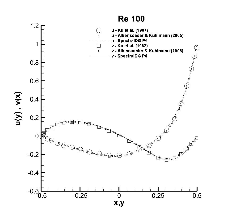
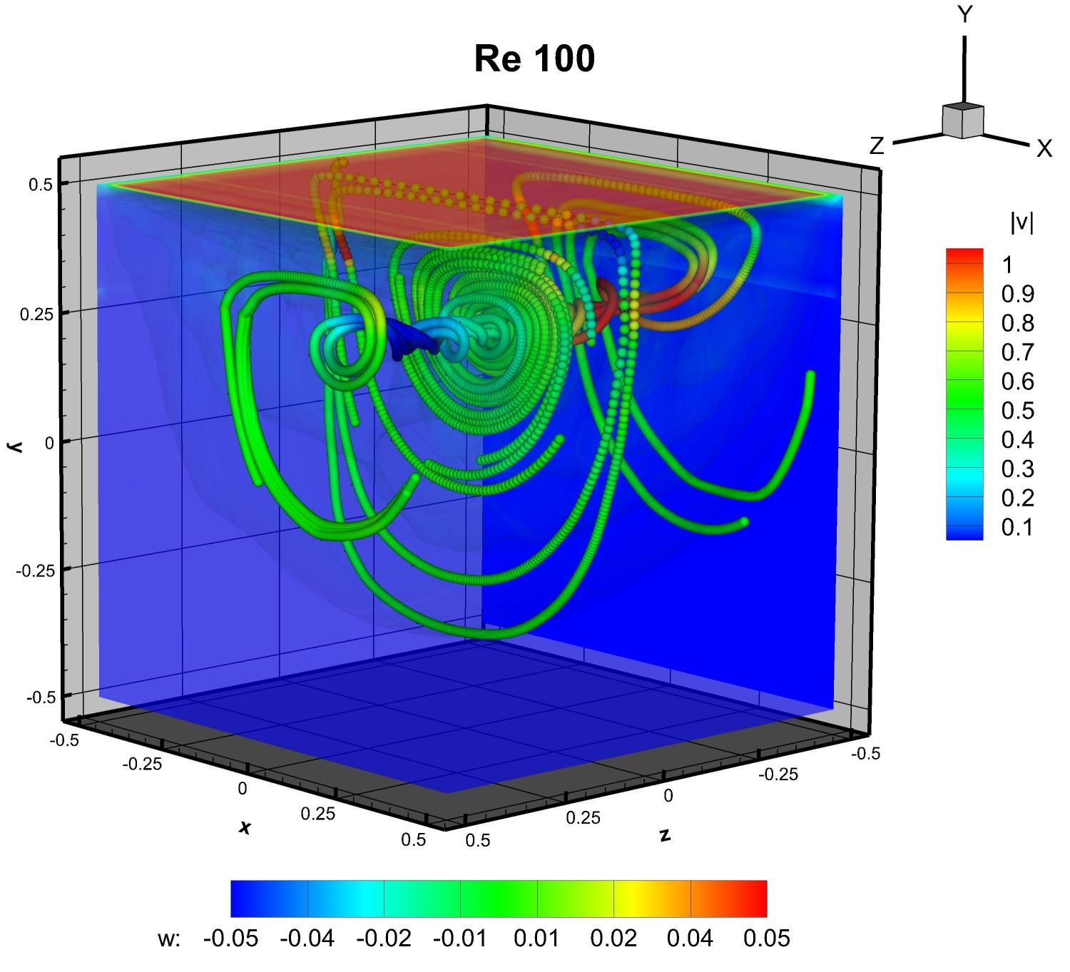
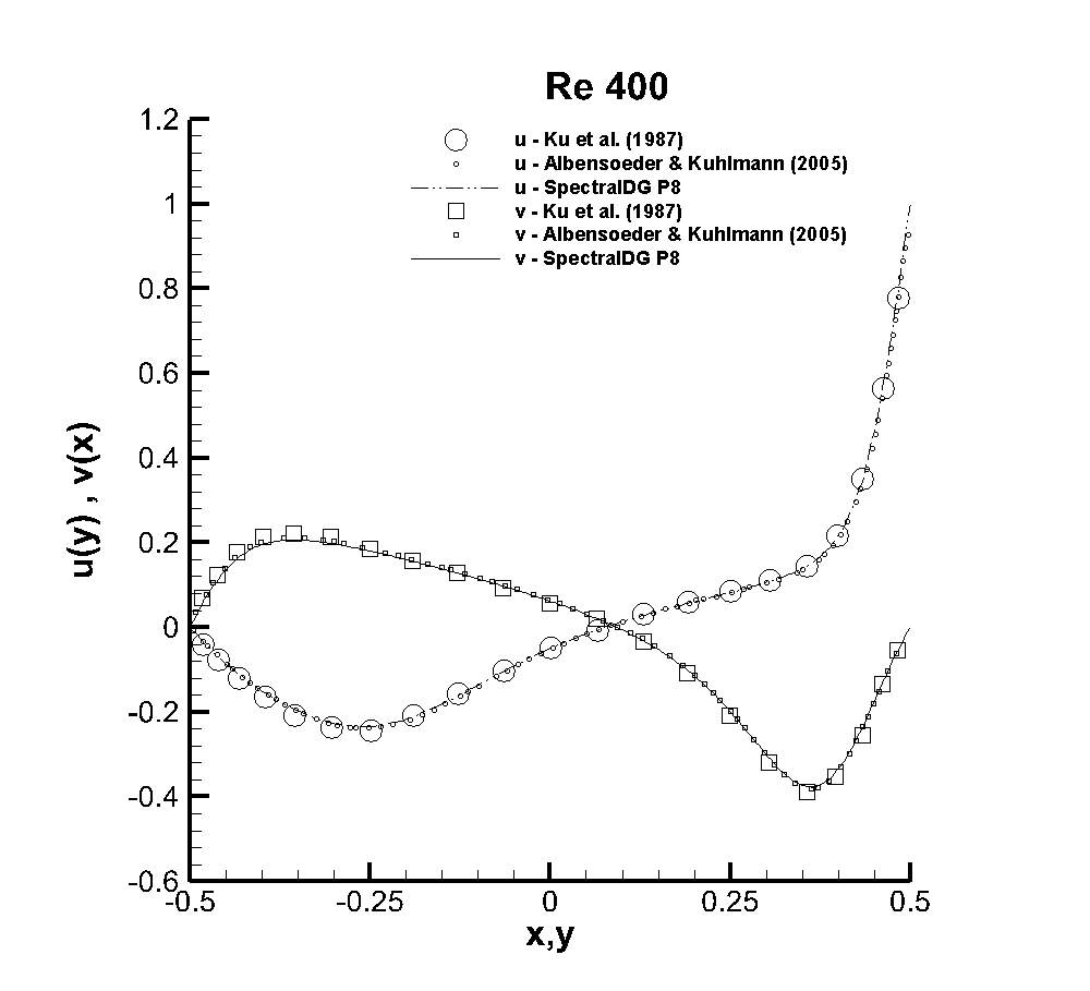
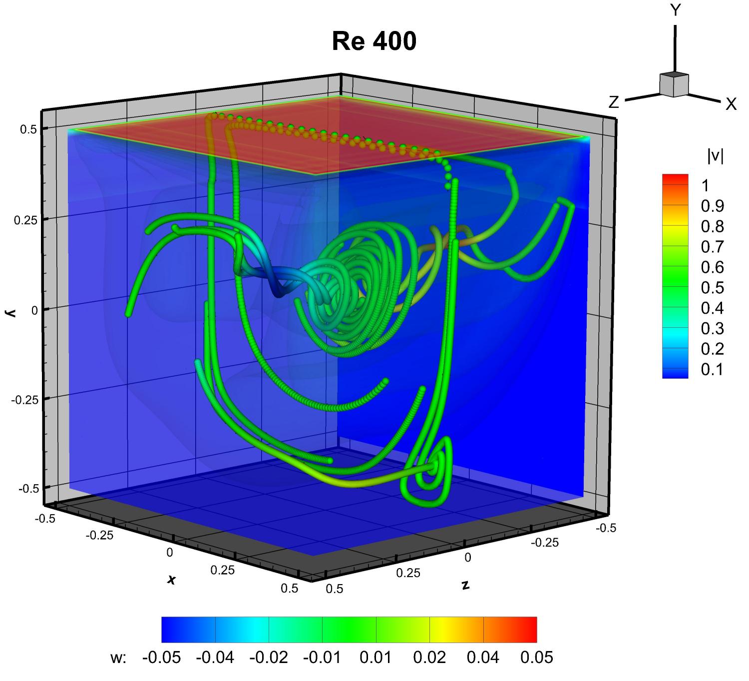
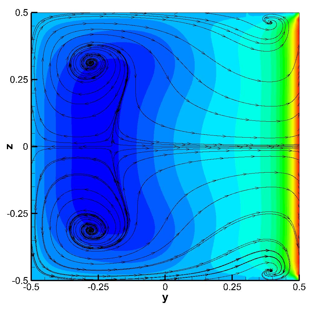
Figure 4: The numerical solution obtained for the three dimensional lid-driven cavity problem compared with the numerical results of [1, 95] at different Reynolds numbers, respectively, from the top to the center: Re=$100$ and Re=$400$ using $5\times 5\times 5$ elements. The results have been obtained with a staggered semi-implicit spectral DG-$\textnormal{P}_{6}$ and DG-$\textnormal{P}_{8}$ method. The streamlines are colored with the $w$ velocity magnitude. The numerical solution for the case $Re=400$ has been interpolated along the three orthogonal planes $x-y$, $x-z$ and $y-z$ at the bottom: streamlines and the $u$ velocity are depicted.

In this section we present the three-dimensional version of the previous test case. A cubic cavity is filled by an incompressible fluid, and the upper wall boundary drives the fluid flow with a non-zero velocity $\mathbf{v}=(1,0,0)$. The presence of a third spatial dimension introduces a new degree of freedom to dynamics of the flow and the resulting flow field is different compared to the 2D case discussed before. The physical domain $\Omega=[-0.5,0.5]^{3}$ has been divided into only $5\times 5\times 5$ spatial elements, with the implicitness factor $\theta=1$ chosen for the time discretization. Fig. 4 shows the computed results compared with the reference data provided by [95] and [1] next to the three-dimensional view of the flow field at Reynolds numbers Re=$100$ and Re=$400$, obtained with the $\textnormal{P}_{6}$ and $\textnormal{P}_{8}$ version of our staggered semi-implicit spectral DG scheme. Also for the three-dimensional cavity flow, our numerical results are in very good agreement with the reference data. At the bottom of Fig. 4 the numerical solution for the case $Re=400$ has been projected onto the three orthogonal planes ${x-y}$, ${x-z}$ and ${y-z}$. The expected secondary recirculations, which distinguish the three dimensional flow field from the two dimensional one, are clearly visible.

2.4.4 Backward facing step: 2D

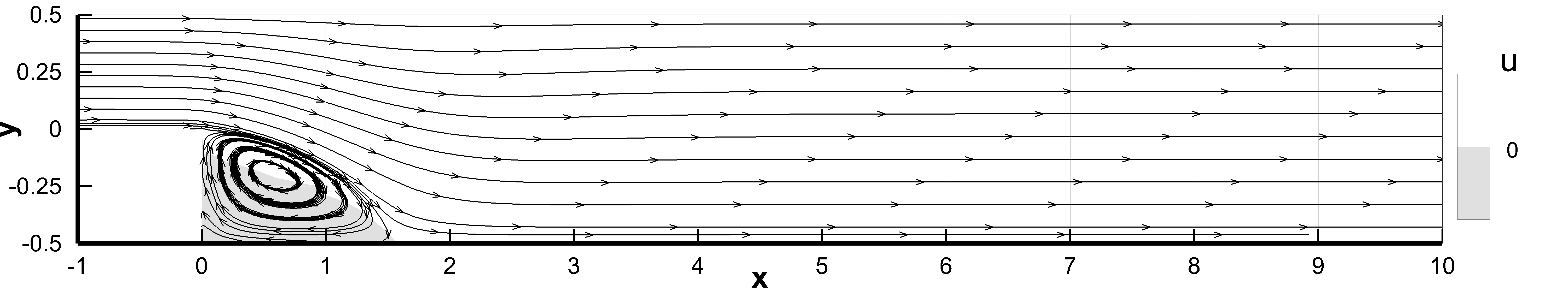
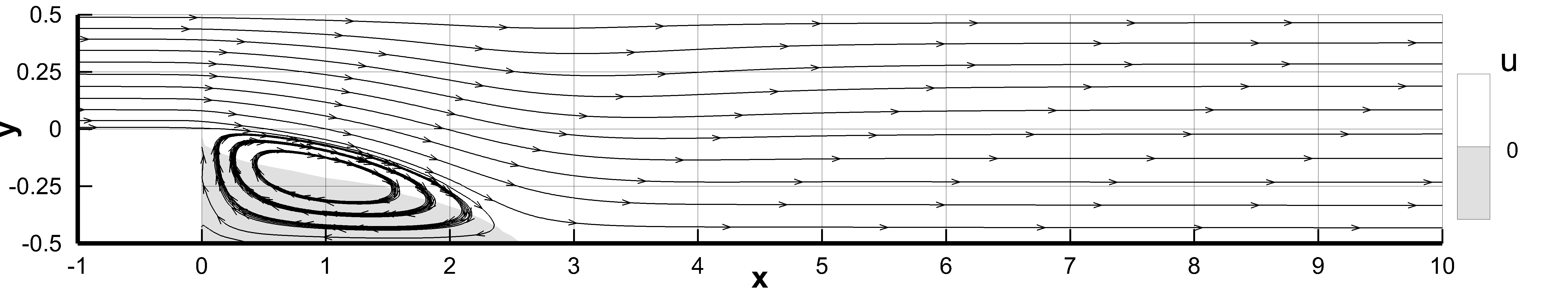
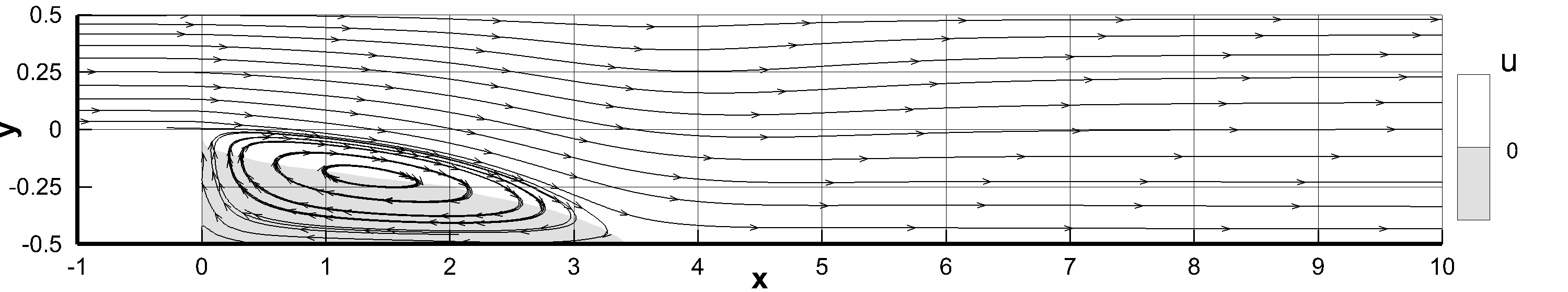
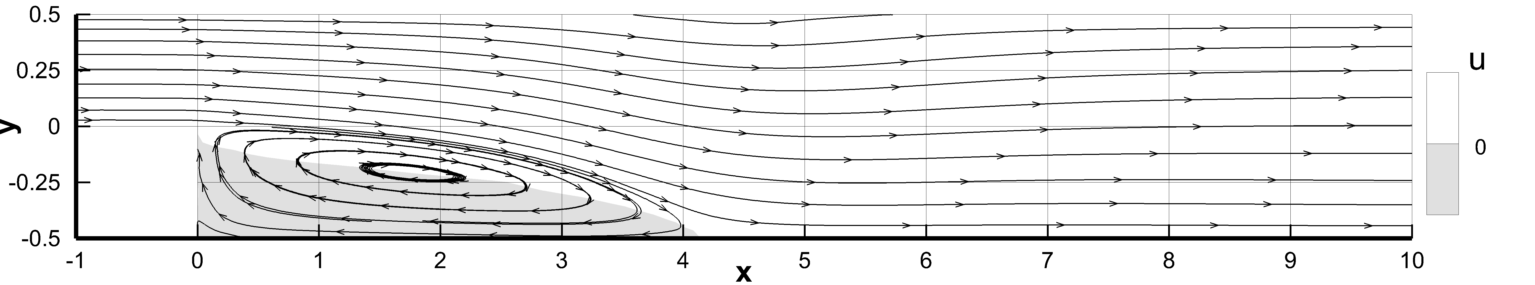
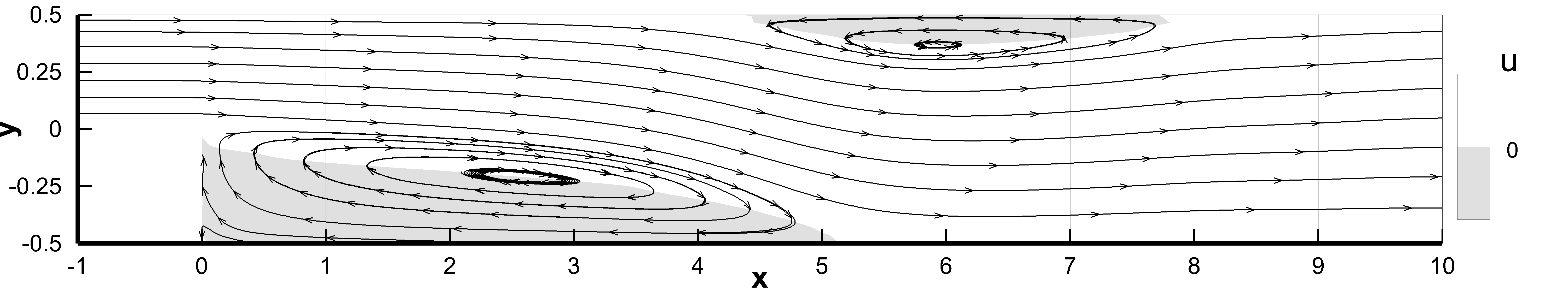
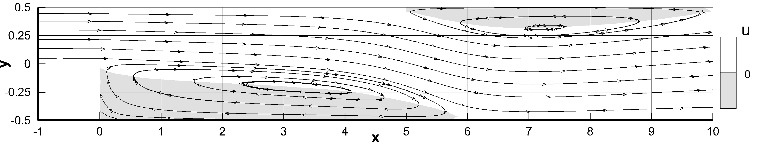
Figure 5: The numerical solution obtained for the two-dimensional backward facing step problem at different Reynolds numbers, respectively, from the top to the bottom: Re=$100$, Re=$200$, Re=$300$, Re=$400$, Re=$500$, Re=$600$, and Re=$800$ obtained with the staggered semi-implicit spectral DG-$\textnormal{P}_{6}$ method. Recirculations are highlighted by the sign of the axial velocity $u$.

Another typical benchmark problem for testing the accuracy of numerical methods in computational fluid dynamics is the backward facing step problem. In this test a flow separation is induced by a sudden backward step inside a two dimensional duct. A main recirculation zone is generated next to the step, starting already at low Reynolds numbers. Then, by increasing the Reynolds number, new secondary recirculations are generated. A non-zero velocity $u=1$ is imposed at the entrance, a constant pressure $p=0$ is imposed at the outflow. In this case the axial spatial domain is $x\in[-10,20]$, the height of the two dimensional duct is $h_{\text{in}}=0.5$ at the entrance and $h_{\text{out}}=h_{\text{in}}+h_{\text{s}}=1.0$ at the exit, with an expansion ratio ER$=h_{\text{out}}/h_{\text{in}}=2$ at $x=0$, i.e. a backward facing step of height $h_{s}=0.5$. The spatial domain is discretized with elements of dimension $\Delta x=1$, $\Delta y=0.25$, the implicitness factor in time is taken as $\theta=0.6$. Fig. 5 shows the streamlines and the recirculation patterns obtained for different Reynolds number up to $Re=800$ with the $\textnormal{P}_{6}$ version of our staggered semi-implicit spectral DG method. The numerical results are compared with the two dimensional reference data provided in [67] and with the experimental measurements of [99]. A good agreement is achieved. The plotted data in Fig. 5 show some discrepancies between the two dimensional simulations and the experimental data [99] that become more visible at higher Reynolds number. These differences are due to three dimensional effects that are introduced by the sidewalls at higher Reynolds numbers, as discussed in [133, 3, 109, 116].

2.4.5 Backward facing step: 3D

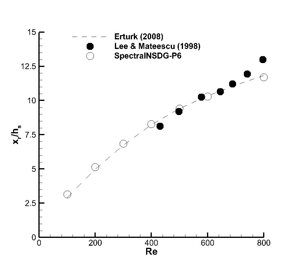
Figure 6: Position of the reattachment point obtained with the staggered semi-implicit spectral DG-$\textnormal{P}_{6}$ method for the two dimensional backward facing step problem compared with the two dimensional numerical results of [67] and the experimental measurements of [99] at different Reynolds numbers, in the range $Re\in(0,800)$.

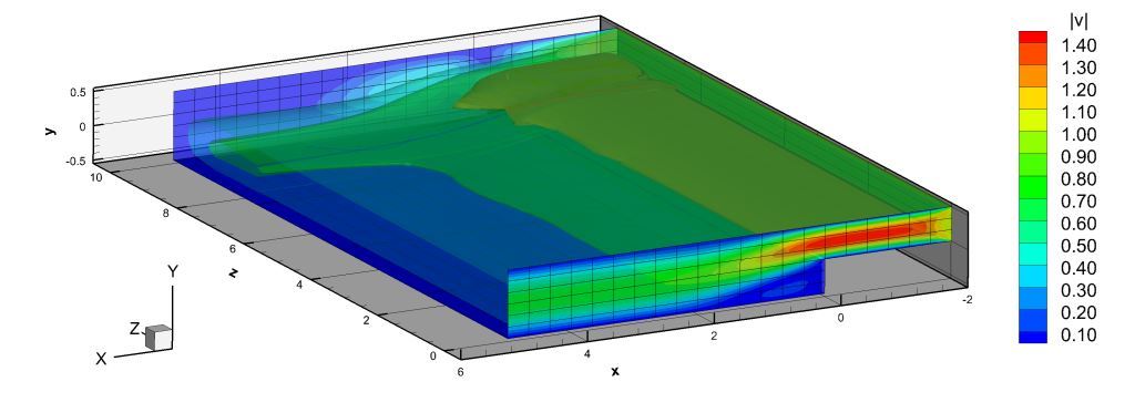
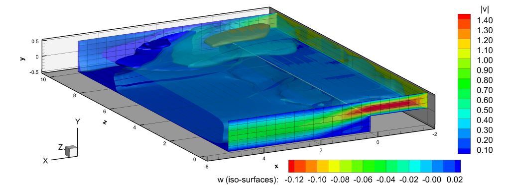
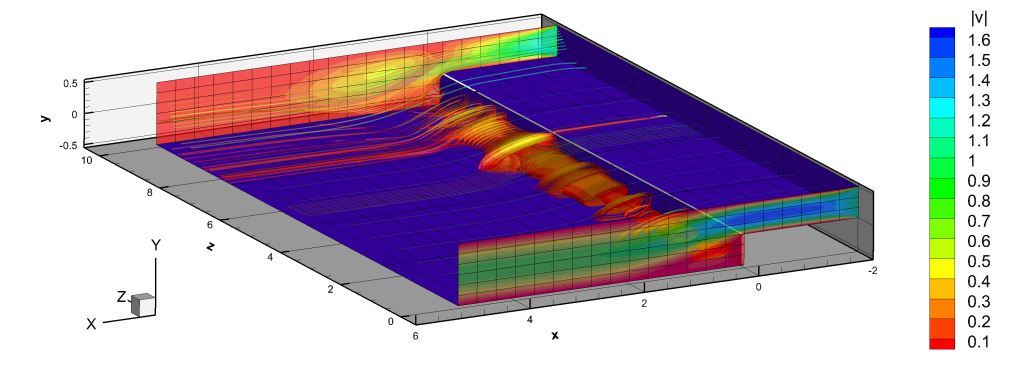
Figure 7: Numerical solution for the three dimensional backward facing step problem at time $t=25.0$ computed with the staggered semi-implicit spectral DG-$\mathbb{P}_{3}$ method for $Re=100$. The iso-surfaces of the velocity magnitude (top), the iso-surfaces of the $w$ velocity component (center) and the streamtraces of the fluid flow (bottom) are plotted for the first half of the spatial domain $z>0$.

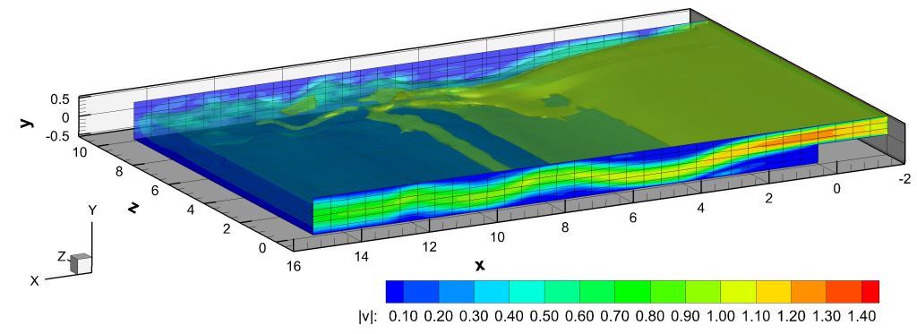
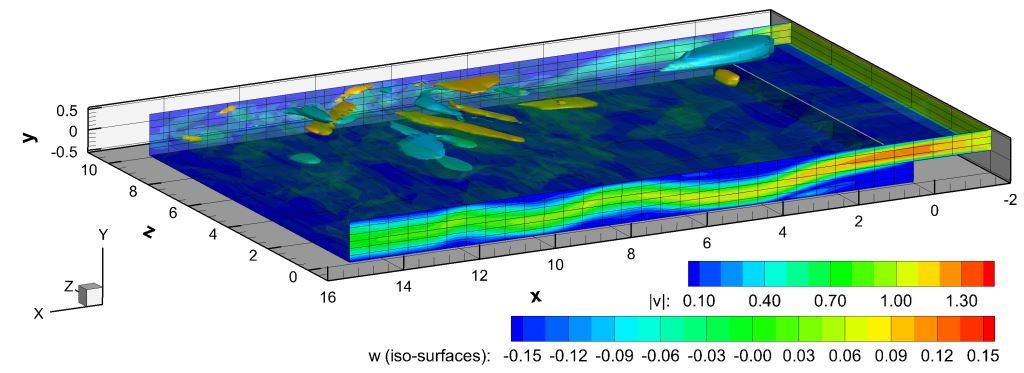
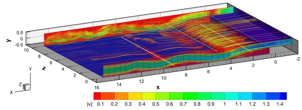
Figure 8: Numerical solution for the three dimensional backward facing step problem at time $t=25.0$ computed with the staggered semi-implicit spectral DG-$\mathbb{P}_{3}$ method for $Re=1000$. The iso-surfaces of the velocity magnitude (top), the iso-surfaces of the $w$ velocity component (center) and the streamtraces of the fluid flow (bottom) are plotted for the first half of the spatial domain $z>0$. The main recirculation axes are highlighted in the figure at the bottom.

In this section, the numerical results of the simulation of the three dimensional extension of the backward facing step problem are shown and discussed. The physical domain is described by an expansion-ratio ER$=2$, and an aspect-ratio AR$=L_{z}/H=40$, where $L_{z}$ is the width of the duct in the third spatial dimension. As mentioned above, the two dimensional results are show differences compared to the experimental data for higher Reynolds numbers. The main reason is that the lateral boundary layers developing on the side walls interact with the main recirculations of the two-dimensional flow. This interpretation is justified by the fact that at lower Reynolds numbers and higher aspect ratio, i.e. when the aforementioned interactions are negligible, the two-dimensional results actually match the three dimensional ones and the experimental data (see Figure 6). The numerical solutions for $Re=100$ (laminar regime) and Re=$1000$ (transitional regime) at time $t=25.0$ obtained with our spectral SIDG-$\textnormal{P}_{3}$ scheme give an overview of the 3D flow field, see Figures 7-8. The friction forces at the lateral boundary layers constrict the axial velocity profile and the main recirculation to the center of the duct. A non-zero $w$ velocity component is generated consequently.

2.5 Three dimensional Taylor-Green vortex problem

A classical fully three-dimensional flow that is widely used for testing the ability of a numerical method in solving the smallest scales in turbulent flows is the three dimensional Taylor-Green vortex problem. In this test the velocity and pressure field are initialized with

$$u(x,y,z,0)=\sin(x)\cos(y)\cos(z),$$ (82)

$$v(x,y,z,0)=-\cos(x)\sin(y)\cos(z),$$ (83)

$$w(x,y,z,0)=0,$$ (84)

$$p(x,y,z,0)=\frac{1}{16}\left(\cos(2x)+\cos(2y)\right)\left(\cos(2z)+2\right).$$ (85)

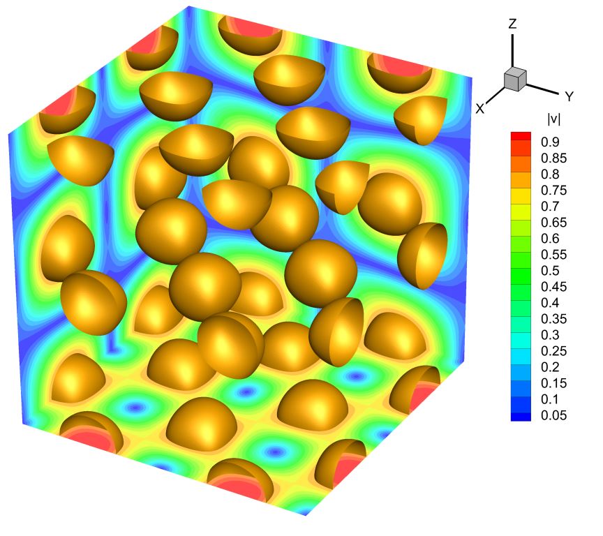
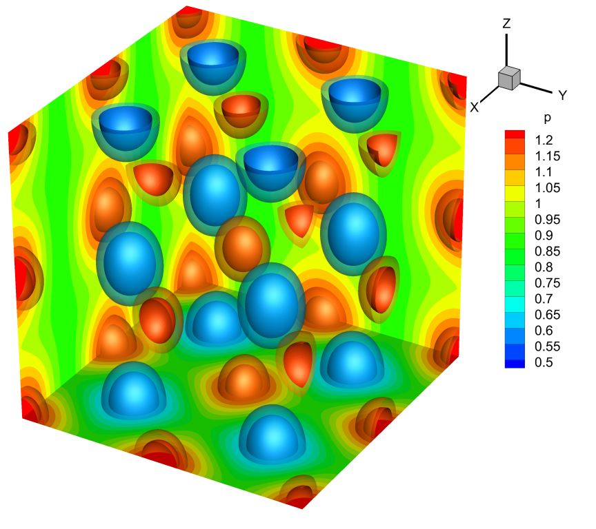
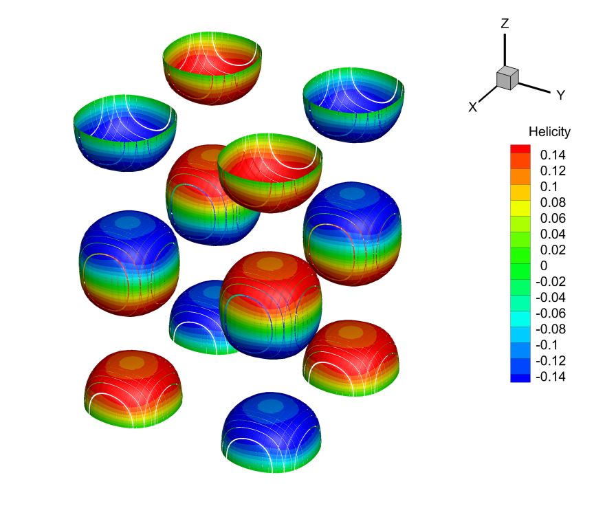
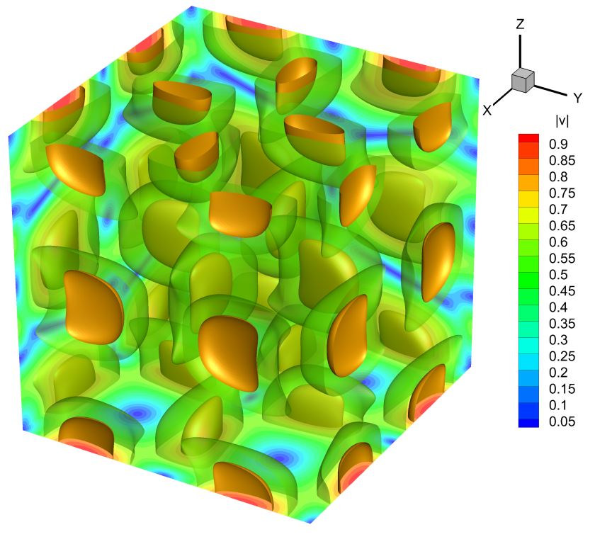
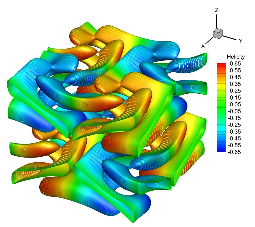
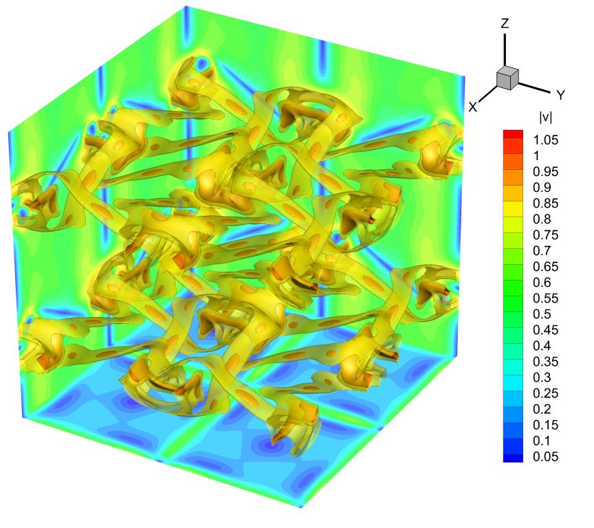
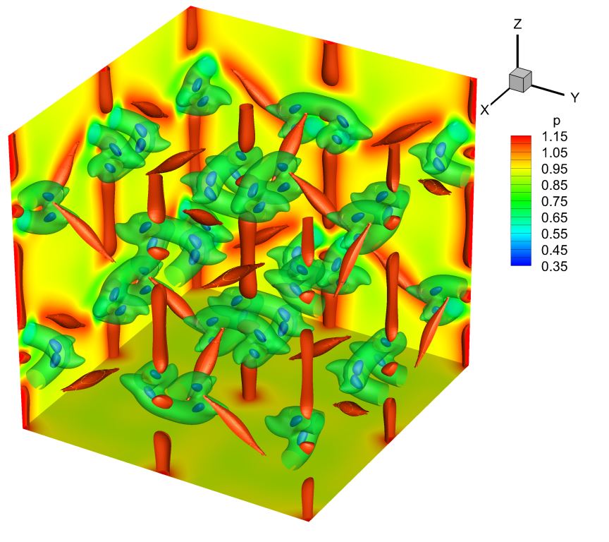
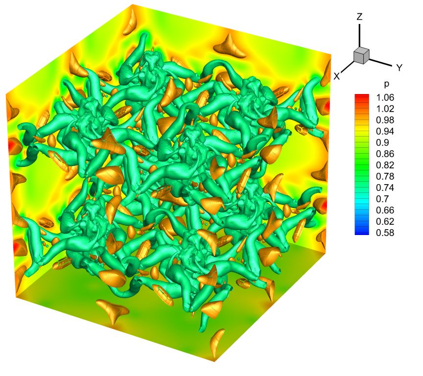
Figure 10: Numerical solution for the three dimensional Taylor-Green vortex flow at $Re=800$ computed with the staggered semi-implicit spectral DG-$\textnormal{P}_{6}$ method using $50^{3}$ elements. The isosurfaces of the velocity (left), the isosurfaces of the pressure (center) and the isosurfaces of the vorticity colored by the helicity field (right) are plotted at times $t=0.4$, $2.0$, $6.0$ and $10.0$ from the top to the bottom, respectively.

The resulting fluid flow is initially smooth and laminar, but the nonlinearity in the governing PDE due to the convective terms combined with a small viscosity quickly generates complex small-scale flow structures after finite times. A widely accepted reference solution for the rate of kinetic energy dissipation has been computed for this test problem by Brachet et al. in [16] through both a direct spectral method based on up to $256^{3}$ modes and a rigorous power series analysis up to order $t^{80}$ (see also [108]). The computational domain is chosen as $\Omega=[0,2\pi]^{3}$, with periodic boundary conditions everywhere. The smaller the expected flow scales, the higher the necessary grid resolution. The time evolution of the main physical variables of the fluid flow is represented in Figure 10 at times $t=0.4$, $2.0$, $6.0$ and $10.0$ for the case $Re=800$. The complexity of the resulting small scale flow structures is clearly visible. In order to compare our results quantitatively with those of Brachet et al. [16], we compute the rate of kinetic energy dissipation

$$\epsilon(t)=-\frac{\partial K}{\partial t}=-\frac{1}{\left\|\Omega\right\|}\frac{\partial}{\partial t}\int_{\Omega}\frac{1}{2}\mathbf{v}^{2}d\mathbf{x}.$$ (86)

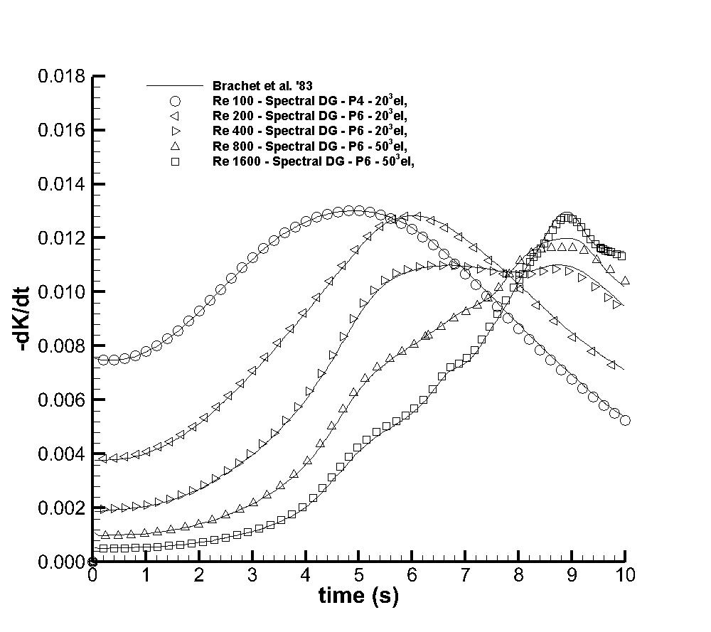
Figure 9: Time evolution of the kinetic energy dissipation rate $\epsilon(t)$ obtained with staggered semi-implicit spectral DG-$\textnormal{P}_{N}$ schemes at different Reynolds numbers $100<Re<1600$. The DNS reference solutions of Brachet et al. [16] are plotted as continuous lines.

Especially when the rate $\epsilon$ reaches its maximum, a high-resolution method together with a sufficiently fine grid is needed in order to resolve the flow physics properly. Figure 9 shows the time evolution of the rate of the global kinetic energy dissipation $\epsilon(t)$ for different Reynolds numbers $Re=100$, Re=$200$, Re=$400$, Re=$800$ and Re=$1600$, obtained with our semi-implicit staggered spectral DG-$\textnormal{P}_{4}$ and -$\textnormal{P}_{6}$ schemes, along with $20^{3}$ and $50^{3}$ elements, respectively, see Figure 9. The computed results fit the DNS reference data very well, confirming that our scheme is able to resolve even the smallest flow scales properly up to $Re=1600$.

3 Spectral space-time DG schemes on staggered Cartesian grids

In this section the high-order DG formulation is extended to the time dimension by looking for discrete solutions $(u_{h},v_{h},w_{h},p_{h})$ under the form of linear combinations of piecewise space-time polynomials of maximum degree $N$ in space and $M$ in time with respect to a reference basis $\mathpzc{B}_{N}$ for the spatial dependency and $\mathpzc{B}_{M}$ for the time dependency. In the following, the general mathematical framework is outlined, and several numerical tests are performed in two and three space dimensions, with the aim of assessing the efficiency and the accuracy of the proposed high order accurate staggered spectral space-time DG scheme.

3.1 Presentation of the numerical scheme

By using the same nomenclature as before, the weak formulation of the governing equations (4-5) in space-time reads

$$\begin{array}[]{lcr}\int\limits_{d\Omega^{*}_{x}\times T_{n+1}}\mathit{f_{u}}\left(\frac{\partial u}{\partial t}+\nabla\cdot\mathbf{F}_{u}+\partial_{x}p\right)=0,&&\\ \int\limits_{d\Omega^{*}_{y}\times T_{n+1}}\mathit{f_{v}}\left(\frac{\partial v}{\partial t}+\nabla\cdot\mathbf{F}_{v}+\partial_{y}p\right)=0,&&\int\limits_{d\Omega\times T_{n+1}}\mathit{f}\,\left(\nabla\cdot\mathbf{v}\right)=0,\\ \int\limits_{d\Omega^{*}_{z}\times T_{n+1}}\mathit{f_{w}}\left(\frac{\partial w}{\partial t}+\nabla\cdot\mathbf{F}_{w}+\partial_{z}p\right)=0,&&\end{array}$$ (90)

where $T_{n+1}=\left[t_{n},t_{n+1}\right]$ is the future time interval where the solution is unknown. Then, the definitions of the piecewise polynomials (6-9) are augmented by

$$\left\{\begin{array}[]{rcl}\hat{u}_{pqr}(t)&=&\sum_{s=0}^{M}\omega_{s}(t)\,\hat{u}_{pqrs},\\ \hat{v}_{pqr}(t)&=&\sum_{s=0}^{M}\omega_{s}(t)\,\hat{v}_{pqrs},\\ \hat{w}_{pqr}(t)&=&\sum_{s=0}^{M}\omega_{s}(t)\,\hat{w}_{pqrs},\\ \hat{p}_{pqr}(t)&=&\sum_{s=0}^{M}\omega_{s}(t)\,\hat{p}_{pqrs},\end{array}\right.\;\;\;\;\;\left.\begin{array}[]{l}\text{with}\;\;t\in T_{n+1},\\ n=1,...,N_{t},\\ u_{lmnp},v_{lmnp},w_{lmnp},p_{lmnp}\in\varmathbb{R},\end{array}\right.$$ (97)

where $\omega_{s}(t)$ is a polynomial in time, generated from the basis functions $\varphi_{s}\in\mathpzc{B}_{M}$ with the rule

$$\omega(t)=\varphi(\xi),\;\;\;\textnormal{with}\;t=t_{n}+\xi\Delta t,\;0\leq\xi\leq 1.$$

Then a staggered space-time DG discretization of the incompressible Navier-Stokes equations reads

$$\int\limits_{T_{i+\frac{1}{2},j,k}\times T_{n+1}}\psi_{m_{1}}(x)\omega_{m_{2}}(y)\omega_{m_{3}}(z)\omega_{m_{0}}(t)\left(\frac{\partial u_{h}}{\partial t}+\nabla\cdot\mathbf{F}_{u}+\partial_{x}p_{h}\right)d\mathbf{x}dt=0,$$ (98)

$$\int\limits_{T_{i,j+\frac{1}{2},k}\times T_{n+1}}\omega_{m_{1}}(x)\psi_{m_{2}}(y)\omega_{m_{3}}(z)\omega_{m_{0}}(t)\left(\frac{\partial v_{h}}{\partial t}+\nabla\cdot\mathbf{F}_{v}+\partial_{y}p_{h}\right)d\mathbf{x}dt=0,$$ (99)

$$\int\limits_{T_{i,j,k+\frac{1}{2}}\times T_{n+1}}\omega_{m_{1}}(x)\omega_{m_{2}}(y)\psi_{m_{3}}(z)\omega_{m_{0}}(t)\left(\frac{\partial w_{h}}{\partial t}+\nabla\cdot\mathbf{F}_{w}+\partial_{z}p_{h}\right)d\mathbf{x}dt=0,$$ (100)

$$\int\limits_{T_{i,j,k}\times T_{n+1}}\omega_{m_{1}}(x)\omega_{m_{2}}(y)\omega_{m_{3}}(z)\omega_{m_{0}}(t)\,\left(\nabla\cdot\mathbf{v}_{h}\right)d\mathbf{x}dt=0.$$ (101)

Again, we need to account for the jump of the pressure inside the velocity control volumes, and we perform integration by parts in space of equation (101), which thus becomes

$$\int\limits_{\partial T_{i,j,k}\times T_{n+1}}\omega_{m_{1}}(x)\omega_{m_{2}}(y)\omega_{m_{3}}(z)\omega_{m_{0}}(t)\,\mathbf{v}_{h}\cdot\vec{n}\,dSdt-\int\limits_{T_{i,j,k}\times T_{n+1}}\nabla\left(\omega_{m_{1}}(x)\omega_{m_{2}}(y)\omega_{m_{3}}(z)\omega_{m_{0}}(t)\right)\cdot\mathbf{v}_{h}(\mathbf{x},t)\,d\mathbf{x}dt=0.$$ (102)

Eqn. (102) is again well defined, since the velocity vector $\mathbf{v}_{h}$ is continuous across the element boundary $\partial T_{i,j,k}\times T_{n+1}$, thanks to the use of a staggered grid approach. Since $p_{h}$ is discontinuous inside the domains of integration of the momentum equations (98-100) the following jump terms arise

$$\int\limits_{t^{n}}^{t^{n+1}}\int\limits_{x_{i}}^{x_{i+1}}\int\limits_{y_{j-\frac{1}{2}}}^{y_{j+\frac{1}{2}}}\int\limits_{z_{k-\frac{1}{2}}}^{z_{k+\frac{1}{2}}}\psi_{m_{1}}(x)\omega_{m_{2}}(y)\omega_{m_{3}}(z)\omega_{m_{0}}(t)\partial_{x}p_{h}(\mathbf{x},t)\,d\mathbf{x}dt=$$

$$\int\limits_{t^{n}}^{t^{n+1}}\int\limits_{x_{i}}^{x_{i+\frac{1}{2}}}\int\limits_{y_{j-\frac{1}{2}}}^{y_{j+\frac{1}{2}}}\int\limits_{z_{k-\frac{1}{2}}}^{z_{k+\frac{1}{2}}}\psi_{m_{1}}(x)\omega_{m_{2}}(y)\omega_{m_{3}}(z)\omega_{m_{0}}(t)\partial_{x}p_{i,j,k}(\mathbf{x},t)\,d\mathbf{x}dt+$$

$$\int\limits_{t^{n}}^{t^{n+1}}\int\limits_{x_{i+\frac{1}{2}}}^{x_{i+1}}\int\limits_{y_{j-\frac{1}{2}}}^{y_{j+\frac{1}{2}}}\int\limits_{z_{k-\frac{1}{2}}}^{z_{k+\frac{1}{2}}}\psi_{m_{1}}(x)\omega_{m_{2}}(y)\omega_{m_{3}}(z)\omega_{m_{0}}(t)\partial_{x}p_{i+1,j,k}(\mathbf{x},t)\,d\mathbf{x}dt+$$

$$+\int\limits_{t^{n}}^{t^{n+1}}\int\limits_{y_{j-\frac{1}{2}}}^{y_{j+\frac{1}{2}}}\int\limits_{z_{k-\frac{1}{2}}}^{z_{k+\frac{1}{2}}}\psi_{m_{1}}(x_{i+\frac{1}{2}})\omega_{m_{2}}(y)\omega_{m_{3}}(z)\omega_{m_{0}}(t)\left(p_{i+1,j,k}(x_{i+\frac{1}{2}},y,z,t)-p_{i,j,k}(x_{i+\frac{1}{2}},y,z,t)\right)dydzdt,$$ (103)

with similar expressions also in the $y$- and $z$-momentum equations, respectively.

The only real changes with respect to the previous formulation arise in the integration of the time derivatives that, after integrating by parts in time and introducing the known solution at time $t^{n}$ (upwinding in time, according to the causality principle), read

$$\!\!\!\!\!\int\limits_{T_{i+\frac{1}{2},j,k}\times T_{n+1}}\!\!\!\!\!\psi_{m_{1}}(x)\omega_{m_{2}}(y)\omega_{m_{3}}(z)\omega_{m_{0}}(t)\frac{\partial u_{h}}{\partial t}d\mathbf{x}dt=\int\limits_{T_{i+\frac{1}{2},j,k}}\!\!\psi_{m_{1}}(x)\omega_{m_{2}}(y)\omega_{m_{3}}(z)\left(\omega_{m_{0}}(t^{n+1})u_{h}(\mathbf{x},t^{n+1})-\omega_{m_{0}}(t^{n})u_{h}(\mathbf{x},t^{n})\right)d\mathbf{x}$$

$$-\int\limits_{T_{i+\frac{1}{2},j,k}\times T_{n+1}}\!\!\!\!\!\psi_{m_{1}}(x)\omega_{m_{2}}(y)\omega_{m_{3}}(z)\left(\frac{\partial}{\partial t}\omega_{m_{0}}(t)\right)u_{h}d\mathbf{x}dt=\mathbf{M}^{\textsl{xyz}}\left[\left(\mathbf{M}^{\textsl{t}}_{1}-\mathbf{M}^{\textsl{t}}_{V}\right)\cdot\widehat{\mathbf{U}}^{n+1}_{i,j,k}-\mathbf{M}^{\textsl{t}}_{0}\cdot\widehat{\mathbf{U}}^{n}_{i,j,k}\right]\times\Delta x\,\Delta y\,\Delta z\,$$ (104)

with analogous terms for $v_{h}$ and $w_{h}$, and where

$$\mathbf{M}^{\textsl{t}}_{1} =\left\{M^{t}_{1\,pq}\right\}_{p,q=0,..,M}=\Bigg{\{}\varphi_{p}(1)\varphi_{q}(1)\Bigg{\}}_{p,q=0,..,M},$$ (105)

$$\mathbf{M}^{\textsl{t}}_{0} =\left\{M^{t}_{0\,pq}\right\}_{p,q=0,..,M}=\Bigg{\{}\varphi_{p}(0)\varphi_{q}(1)\Bigg{\}}_{p,q=0,..,M},$$ (106)

$$\mathbf{M}^{\textsl{t}}_{V} =\left\{M^{t}_{V\,pq}\right\}_{p,q=0,..,M}=\left\{\int\limits_{0}^{1}\varphi^{\prime}_{p}(\xi)\varphi_{q}(\xi)\,d\xi\right\}_{p,q=0,..,M}.$$ (107)

With the aim of simplifying the notation, one can extend the spatial $xyz$-formalism of the tensor products (21-24) to the space-time case by defining a generic vector of space-time degrees of freedom as

$$\widehat{\mathbf{X}}=\left\{\hat{x}_{mm^{\prime}m^{\prime\prime}m^{\prime\prime\prime}}\right\}_{m,m^{\prime},m^{\prime\prime}=0,..,N;\,m^{\prime\prime\prime}=0,..,M},$$ (108)

the space-time operators in the form of

$$\begin{array}[]{rl}\mathbf{Z}^{\textsl{x${}_{i}$ x${}_{j}$}}&\equiv\mathbf{Z}^{\textsl{x${}_{i}$}}\cdot\mathbf{Z}^{\textsl{x${}_{j}$}},\\ \mathbf{Z}^{\textsl{x${}_{i}$ x${}_{j}$ x${}_{k}$}}&\equiv\mathbf{Z}^{\textsl{x${}_{i}$}}\cdot\mathbf{Z}^{\textsl{x${}_{j}$}}\cdot\mathbf{Z}^{\textsl{x${}_{k}$}},\\ \mathbf{Z}^{\textsl{x${}_{i}$ x${}_{j}$ x${}_{k}$ x${}_{l}$}}&\equiv\mathbf{Z}^{\textsl{x${}_{i}$}}\cdot\mathbf{Z}^{\textsl{x${}_{j}$}}\cdot\mathbf{Z}^{\textsl{x${}_{k}$}}\cdot\mathbf{Z}^{\textsl{x${}_{l}$}},\end{array}\;\;\;\text{with}\;x_{i},x_{j},x_{k},x_{l}\in\left\{x,y,z,t\right\}$$ (112)

which operate along a generic vector of degrees of freedom via the tensor products

$$\mathbf{Z}^{\textsl{x}}\cdot\widehat{\mathbf{X}}=Z_{ml}I_{m^{\prime}l^{\prime}}I_{m^{\prime\prime}l^{\prime\prime}}I_{m^{\prime\prime\prime}l^{\prime\prime\prime}}x_{l\,l^{\prime}l^{\prime\prime}l^{\prime\prime\prime}},\qquad\mathbf{Z}^{\textsl{y}}\cdot\widehat{\mathbf{X}}=I_{ml}Z_{m^{\prime}l^{\prime}}I_{m^{\prime\prime}l^{\prime\prime}}I_{m^{\prime\prime\prime}l^{\prime\prime\prime}}x_{l\,l^{\prime}l^{\prime\prime}l^{\prime\prime\prime}},$$ (113)

$$\mathbf{Z}^{\textsl{z}}\cdot\widehat{\mathbf{X}}=I_{ml}I_{m^{\prime}l^{\prime}}Z_{m^{\prime\prime}l^{\prime\prime}}I_{m^{\prime\prime\prime}l^{\prime\prime\prime}}x_{l\,l^{\prime}l^{\prime\prime}l^{\prime\prime\prime}},\qquad\mathbf{Z}^{\textsl{t}}\cdot\widehat{\mathbf{X}}=I_{ml}I_{m^{\prime}l^{\prime}}I_{m^{\prime\prime}l^{\prime\prime}}Z_{m^{\prime\prime\prime}l^{\prime\prime\prime}}x_{l\,l^{\prime}l^{\prime\prime}l^{\prime\prime\prime}},$$ (114)

where $\mathbf{Z}$ is a real square matrix, $I$ is the identity operator and the Einstein convention of summation over repeated indexes is assumed. In this notation the mass matrix that corresponds to the time coordinate can be written as $\mathbf{M}^{\textsl{t}}$, according to the definition of the mass matrix in equations (20). Then, from equations (98-101) the following system is obtained:

$$\mathbf{M}^{\textsl{xyz}}\left[\left(\mathbf{M}^{\textsl{t}}_{1}-\mathbf{M}^{\textsl{t}}_{V}\right)\cdot\widehat{\mathbf{U}}^{n+1}_{i+\frac{1}{2},j,k}-\mathbf{M}^{\textsl{t}}_{0}\cdot\widehat{\mathbf{Fu}}^{n}_{i+\frac{1}{2},j,k}\right]+\frac{\Delta t}{\Delta x}\mathbf{M}^{\textsl{yzt}}\cdot\left(\mathbf{R}_{\text{{{v}}}}^{\textsl{x}}\cdot\widehat{\mathbf{P}}^{n+1}_{i+1,j,k}-\mathbf{L}_{\text{{{v}}}}^{\textsl{x}}\cdot\widehat{\mathbf{P}}^{n+1}_{i,j,k}\right) =0,$$ (115)

$$\mathbf{M}^{\textsl{xyz}}\left[\left(\mathbf{M}^{\textsl{t}}_{1}-\mathbf{M}^{\textsl{t}}_{V}\right)\cdot\widehat{\mathbf{V}}^{n+1}_{i,j+\frac{1}{2},k}-\mathbf{M}^{\textsl{t}}_{0}\cdot\widehat{\mathbf{Fv}}^{n}_{i,j+\frac{1}{2},k}\right]+\frac{\Delta t}{\Delta y}\mathbf{M}^{\textsl{zxt}}\cdot\left(\mathbf{R}_{\text{{{v}}}}^{\textsl{y}}\cdot\widehat{\mathbf{P}}^{n+1}_{i,j+1,k}-\mathbf{L}_{\text{{{v}}}}^{\textsl{y}}\cdot\widehat{\mathbf{P}}^{n+1}_{i,j,k}\right) =0,$$ (116)

$$\mathbf{M}^{\textsl{xyz}}\left[\left(\mathbf{M}^{\textsl{t}}_{1}-\mathbf{M}^{\textsl{t}}_{V}\right)\cdot\widehat{\mathbf{W}}^{n+1}_{i,j,k+\frac{1}{2}}-\mathbf{M}^{\textsl{t}}_{0}\cdot\widehat{\mathbf{Fw}}^{n}_{i,j,k+\frac{1}{2}}\right]+\frac{\Delta t}{\Delta z}\mathbf{M}^{\textsl{xyt}}\cdot\left(\mathbf{R}_{\text{{{v}}}}^{\textsl{z}}\cdot\widehat{\mathbf{P}}^{n+1}_{i,j,k+1}-\mathbf{L}_{\text{{{v}}}}^{\textsl{z}}\cdot\widehat{\mathbf{P}}^{n+1}_{i,j,k}\right) =0,$$ (117)

$$\frac{\mathbf{M}^{\textsl{yzt}}\left(\mathbf{R}_{\text{{{p}}}}^{\textsl{x}}\cdot\widehat{\mathbf{U}}^{n+1}_{i+\frac{1}{2},j,k}\!-\!\mathbf{L}_{\text{{{p}}}}^{\textsl{x}}\cdot\widehat{\mathbf{U}}^{n+1}_{i-\frac{1}{2},j,k}\right)}{\Delta x}+\frac{\mathbf{M}^{\textsl{zxt}}\left(\mathbf{R}_{\text{{{p}}}}^{\textsl{y}}\cdot\widehat{\mathbf{V}}^{n+1}_{i,j+\frac{1}{2},k}\!-\!\mathbf{L}_{\text{{{p}}}}^{\textsl{y}}\cdot\widehat{\mathbf{V}}^{n+1}_{i,j-\frac{1}{2},k}\right)}{\Delta y}+\frac{\mathbf{M}^{\textsl{xyt}}\left(\mathbf{R}_{\text{{{p}}}}^{\textsl{z}}\cdot\widehat{\mathbf{W}}^{n+1}_{i,j,k+\frac{1}{2}}\!-\!\mathbf{L}_{\text{{{p}}}}^{\textsl{z}}\cdot\widehat{\mathbf{W}}^{n+1}_{i,j,k-\frac{1}{2}}\right)}{\Delta z}=0,$$ (118)

which is analogous to the system of equations (16-19), where now the advective-diffusive terms are computed according to

$$\mathbf{M}^{\textsl{t}}_{0}\cdot\widehat{\mathbf{Fu}}^{n}_{i,j,k} =\mathbf{M}^{\textsl{t}}_{0}\cdot\widehat{\mathbf{U}}^{n}_{i,j,k}-\frac{\Delta t}{\Delta x\Delta y\Delta z}\left(\mathbf{M}^{\textsl{xyz}}\right)^{-1}\mathbf{M}^{\textsl{t}}\cdot\left(\,\int\limits_{\partial T_{i,j,k}}\omega\mathbf{F}_{u}\cdot\vec{n}dS-\int\limits_{T_{i,j,k}}\nabla\omega\cdot\mathbf{F}_{u}\,d\mathbf{x}\right),$$ (119)

$$\mathbf{M}^{\textsl{t}}_{0}\cdot\widehat{\mathbf{Fv}}^{n}_{i,j,k} =\mathbf{M}^{\textsl{t}}_{0}\cdot\widehat{\mathbf{V}}^{n}_{i,j,k}-\frac{\Delta t}{\Delta x\Delta y\Delta z}\left(\mathbf{M}^{\textsl{xyz}}\right)^{-1}\mathbf{M}^{\textsl{t}}\cdot\left(\,\int\limits_{\partial T_{i,j,k}}\omega\mathbf{F}_{v}\cdot\vec{n}dS-\int\limits_{T_{i,j,k}}\nabla\omega\cdot\mathbf{F}_{v}\,d\mathbf{x}\right),$$ (120)

$$\mathbf{M}^{\textsl{t}}_{0}\cdot\widehat{\mathbf{Fw}}^{n}_{i,j,k} =\mathbf{M}^{\textsl{t}}_{0}\cdot\widehat{\mathbf{W}}^{n}_{i,j,k}-\frac{\Delta t}{\Delta x\Delta y\Delta z}\left(\mathbf{M}^{\textsl{xyz}}\right)^{-1}\mathbf{M}^{\textsl{t}}\cdot\left(\,\int\limits_{\partial T_{i,j,k}}\omega\mathbf{F}_{w}\cdot\vec{n}dS-\int\limits_{T_{i,j,k}}\nabla\omega\cdot\mathbf{F}_{w}\,d\mathbf{x}\right).$$ (121)

The adopted numerical strategy for the implicit diffusion is actually the higher order time extension of the aforementioned implicit approach and it will be described later in this section. Following the philosophy of section 2, after multiplying equations (115-117) by the inverse of the matrix $\mathbf{M}^{\textsl{xyz}}\left(\mathbf{M}^{\textsl{t}}_{1}-\mathbf{M}^{\textsl{t}}_{V}\right)$, the following direct definitions of the degrees of freedom of the velocity components are obtained

$$\widehat{\mathbf{U}}^{n+1}_{i+\frac{1}{2},j,k} =\left(\mathbf{M}^{\textsl{t}}_{1}-\mathbf{M}^{\textsl{t}}_{V}\right)^{-1}\mathbf{M}^{\textsl{t}}_{0}\cdot\widehat{\mathbf{Fu}}^{n}_{i+\frac{1}{2},j,k}{-}\frac{\Delta t}{\Delta x}\left(\mathbf{M}^{\textsl{t}}_{1}-\mathbf{M}^{\textsl{t}}_{V}\right)^{-1}\mathbf{M}^{\textsl{t}}\left(\mathbf{M}^{\textsl{x}}\right)^{-1}\cdot\left(\mathbf{R}_{\text{{{v}}}}^{\textsl{x}}\cdot\widehat{\mathbf{P}}^{n+1}_{i+1,j,k}-\mathbf{L}_{\text{{{v}}}}^{\textsl{x}}\cdot\widehat{\mathbf{P}}^{n+1}_{i,j,k}\right),$$ (122)

$$\widehat{\mathbf{V}}^{n+1}_{i,j+\frac{1}{2},k} =\left(\mathbf{M}^{\textsl{t}}_{1}-\mathbf{M}^{\textsl{t}}_{V}\right)^{-1}\mathbf{M}^{\textsl{t}}_{0}\cdot\widehat{\mathbf{Fv}}^{n}_{i,j+\frac{1}{2},k}{-}\frac{\Delta t}{\Delta y}\left(\mathbf{M}^{\textsl{t}}_{1}-\mathbf{M}^{\textsl{t}}_{V}\right)^{-1}\mathbf{M}^{\textsl{t}}\left(\mathbf{M}^{\textsl{y}}\right)^{-1}\cdot\left(\mathbf{R}_{\text{{{v}}}}^{\textsl{y}}\cdot\widehat{\mathbf{P}}^{n+1}_{i,j+1,k}-\mathbf{L}_{\text{{{v}}}}^{\textsl{y}}\cdot\widehat{\mathbf{P}}^{n+1}_{i,j,k}\right),$$ (123)

$$\widehat{\mathbf{W}}^{n+1}_{i,j,k+\frac{1}{2}} =\left(\mathbf{M}^{\textsl{t}}_{1}-\mathbf{M}^{\textsl{t}}_{V}\right)^{-1}\mathbf{M}^{\textsl{t}}_{0}\cdot\widehat{\mathbf{Fw}}^{n}_{i,j,k+\frac{1}{2}}{-}\frac{\Delta t}{\Delta z}\left(\mathbf{M}^{\textsl{t}}_{1}-\mathbf{M}^{\textsl{t}}_{V}\right)^{-1}\mathbf{M}^{\textsl{t}}\left(\mathbf{M}^{\textsl{z}}\right)^{-1}\cdot\left(\mathbf{R}_{\text{{{v}}}}^{\textsl{z}}\cdot\widehat{\mathbf{P}}^{n+1}_{i,j,k+1}-\mathbf{L}_{\text{{{v}}}}^{\textsl{z}}\cdot\widehat{\mathbf{P}}^{n+1}_{i,j,k}\right),$$ (124)

Then, after substitution of the resulting equations in the discrete incompressibility condition (118), one obtains

$$\left[\mathbf{M}^{\textsl{t}}\left(\mathbf{M}^{\textsl{t}}_{1}-\mathbf{M}^{\textsl{t}}_{V}\right)^{-1}\mathbf{M}^{\textsl{t}}\;\;\mathbb{H}^{i,j,k}\right]\cdot\mathpzc{P}^{n+1}=\left[\mathbf{M}^{\textsl{t}}\left(\mathbf{M}^{\textsl{t}}_{1}-\mathbf{M}^{\textsl{t}}_{V}\right)^{-1}\mathbf{M}^{\textsl{t}}_{0}\right]\cdot\mathpzc{b}^{n}_{i,j,k}$$ (125)

that is the higher order time-accurate version of the pressure equation, analogous to (25). The right hand side $\mathpzc{b}^{n}_{i,j,k}$ collects all the known terms, i.e. the advective and diffusive terms $\{\widehat{\mathbf{Fu}}^{n}\}$, $\{\widehat{\mathbf{Fv}}^{n}\}$ and $\{\widehat{\mathbf{Fw}}^{n}\}$. This system is not symmetric because of the non-symmetric time-matrices (105) and (107). After multiplication by the inverse of $\mathbf{M}^{\textsl{t}}\left(\mathbf{M}^{\textsl{t}}_{1}-\mathbf{M}^{\textsl{t}}_{V}\right)^{-1}$, the non-symmetric contribution of the time-matrix can be removed, and the same well suited coefficient matrix $\mathbb{H}$ of section 2 is obtained, i.e.

$$\mathbf{M}^{\textsl{t}}\mathbb{H}^{i,j,k}\cdot\mathpzc{P}^{n+1}=\left[\mathbf{M}^{\textsl{t}}_{0}\right]\cdot\mathpzc{b}^{n}_{i,j,k}$$ (126)

and consequently, the resulting system is symmetric and strictly positive definite (for appropriate pressure boundary conditions). Hence, it can be solved very efficiently by means of a classical conjugate gradient method. Once the system for the higher order accurate space-time expansion coefficients of the pressure $\mathpzc{P}^{n+1}$ has been solved, the velocity can be readily updated according to equations (122-124). Note, however, that although the presented space-time DG framework is formally high order accurate in time, the final numerical scheme is strongly influenced by the time-splitting between advection, diffusion and incompressibility condition, which constrains the final method to be only first order accurate in time. In section 3.3 a very simple numerical procedure based on the Picard iteration is outlined in order to circumvent the order limitation induced by the time-splitting and to enable the final solution to preserve the original high-order time accuracy of the presented spectral staggered space-time DG discretization.

3.2 Implicit diffusion

Following the same procedure outlined in Section 2, the high-order time accurate version of the implicit scheme for diffusion (69) reads

$$\mathbf{M}^{\textsl{xyz}}\cdot\left[\left(\mathbf{M}^{\textsl{t}}_{1}-\mathbf{M}^{\textsl{t}}_{V}\right)\cdot\widehat{\mathbf{U}}^{n+1}_{i,j,k}-\mathbf{M}^{\textsl{t}}_{0}\cdot\widehat{\mathbf{Fu}}^{n}_{i,j,k}\right]-\frac{\Delta t}{\Delta x}\mathbf{M}^{\textsl{yzt}}\cdot\left(\mathbf{R}_{\text{{{p}}}}^{\textsl{x}}\cdot\widehat{\mathbf{U}}^{\textsl{(x)}}_{i+\frac{1}{2},j,k}-\mathbf{L}_{\text{{{p}}}}^{\textsl{x}}\cdot\widehat{\mathbf{U}}^{\textsl{(x)}}_{i-\frac{1}{2},j,k}\right)+$$

$$-\frac{\Delta t}{\Delta y}\mathbf{M}^{\textsl{zxt}}\cdot\left(\mathbf{R}_{\text{{{p}}}}^{\textsl{y}}\cdot\widehat{\mathbf{U}}^{\textsl{(y)}}_{i,j+\frac{1}{2},k}-\mathbf{L}_{\text{{{p}}}}^{\textsl{y}}\cdot\widehat{\mathbf{U}}^{\textsl{(y)}}_{i,j-\frac{1}{2},k}\right)-\frac{\Delta t}{\Delta z}\mathbf{M}^{\textsl{xyt}}\cdot\left(\mathbf{R}_{\text{{{p}}}}^{\textsl{z}}\cdot\widehat{\mathbf{U}}^{\textsl{(z)}}_{i,j,k+\frac{1}{2}}-\mathbf{L}_{\text{{{p}}}}^{\textsl{z}}\cdot\widehat{\mathbf{U}}^{\textsl{(z)}}_{i,j,k-\frac{1}{2}}\right)=0,$$ (127)

Then, after substituting the definitions of the velocity derivatives (70-72) the high-order accurate space-time DG version of (73) can be written as

$$\left[\left(\mathbb{M}^{t}_{1}-\mathbb{M}^{t}_{V}\right)\mathbb{M}^{xyz}+\nu\mathbb{M}^{t}\mathbb{H}^{xyz}\right]\cdot\mathpzc{U}= \mathbb{M}^{t}_{0}\mathbb{M}^{xyz}\cdot\mathpzc{Fu}^{n},$$

$$\left[\left(\mathbb{M}^{t}_{1}-\mathbb{M}^{t}_{V}\right)\mathbb{M}^{xyz}+\nu\mathbb{M}^{t}\mathbb{H}^{xyz}\right]\cdot\mathpzc{V}= \mathbb{M}^{t}_{0}\mathbb{M}^{xyz}\cdot\mathpzc{Fv}^{n},$$

$$\left[\left(\mathbb{M}^{t}_{1}-\mathbb{M}^{t}_{V}\right)\mathbb{M}^{xyz}+\nu\mathbb{M}^{t}\mathbb{H}^{xyz}\right]\cdot\mathpzc{W}= \mathbb{M}^{t}_{0}\mathbb{M}^{xyz}\cdot\mathpzc{Fw}^{n},$$ (128)

that is non-symmetric because of the time-matrices

$$\left(\mathbb{M}^{t}_{1}-\mathbb{M}^{t}_{V}\right)=\left\{\left(\mathbf{M}^{\textsl{t}}_{1}-\mathbf{M}^{\textsl{t}}_{V}\right)_{ijk}\right\},\hskip 28.45274pt\mathbb{M}^{t}_{0}=\left\{\left.\mathbf{M}^{\textsl{t}}_{0}\right._{ijk}\right\}$$ (129)

and can be efficiently solved by means of a classical GMRES method [119]. Notice that the non-symmetric component of system (128) can be shifted to the viscous terms, i.e. the second term on the left-hand-side, by multiplying the equations with the inverse of $\left(\mathbb{M}^{t}_{1}-\mathbb{M}^{t}_{V}\right)$ from the left. In that case, for small viscosities, the system can be seen as a non-symmetric perturbation of the inviscid case.

3.3 Space-time pressure correction algorithm

In Section 2 the final staggered semi-implicit DG scheme (79-77) consists of two main blocks that are solved sequentially by the use of a fractional time-step approach. If only high order of accuracy in space is needed, such a splitting is possible. The first fractional block is described by the discrete advection-diffusion equations (75-77), which itself contains a first fractional step for the purely explicit advection and a second fractional step for the implicit discretization of the diffusive terms. Then, the second fractional block contains the solution of the discrete pressure Poisson equation that results from substituting the discrete momentum equations into the discrete incompressibility condition, i.e. combining (79-81) with (78). The important fact is that the chosen fractional time discretization is only first order accurate. In principle, higher order schemes for fractional time-stepping or other more sophisticated techniques could be adopted in defiance of simplicity or generality [87, 141, 88, 104]. In this work a simple Picard method has been implemented. In this manner, the first order time-splitting approach of system (79-77) can then be generalized to arbitrary high order of accuracy in time at the aid of the Picard procedure. We emphasize that at the moment we have no rigorous mathematical proof for the fact that the Picard iterations actually increase the order of accuracy by one per iteration. We only have numerical evidence which support this claim in the context of high order ADER schemes, see [58], as well as the numerical convergence tables shown later in this paper for a set of test cases. The final version of the spectral staggered space-time DG scheme, which is written in terms of a space-time pressure correction algorithm, reads: for $k=0,\ldots,M$ do

$$\left[\left(\mathbb{M}^{t}_{1}-\mathbb{M}^{t}_{V}\right)\mathbb{M}^{xyz}+\nu\mathbb{M}^{t}\mathbb{H}^{xyz}\right]\cdot\mathpzc{U}_{\#}^{{n+1,(k+\frac{1}{2})}}= \mathbb{M}^{xyz}\cdot\left[\mathbb{M}^{t}_{0}\cdot\mathpzc{Fu}^{n+1,(k)}_{\#}-{\pi_{:*\rightarrow\#}}\left\{\frac{\Delta t}{\Delta x}\mathbb{M}^{t}\cdot\left(\mathbb{M}^{-1}\mathcal{D}\right)^{x}\cdot\mathpzc{P}^{n+1,(k)}_{{\#}}\right\}\right],$$ (130)

$$\left[\left(\mathbb{M}^{t}_{1}-\mathbb{M}^{t}_{V}\right)\mathbb{M}^{xyz}+\nu\mathbb{M}^{t}\mathbb{H}^{xyz}\right]\cdot\mathpzc{V}_{\#}^{{n+1,(k+\frac{1}{2})}}= \mathbb{M}^{xyz}\cdot\left[\mathbb{M}^{t}_{0}\cdot\mathpzc{Fv}^{n+1,(k)}_{\#}-{\pi_{:*\rightarrow\#}}\left\{\frac{\Delta t}{\Delta y}\mathbb{M}^{t}\cdot\left(\mathbb{M}^{-1}\mathcal{D}\right)^{y}\cdot\mathpzc{P}^{n+1,(k)}_{{\#}}\right\}\right],$$ (131)

$$\left[\left(\mathbb{M}^{t}_{1}-\mathbb{M}^{t}_{V}\right)\mathbb{M}^{xyz}+\nu\mathbb{M}^{t}\mathbb{H}^{xyz}\right]\cdot\mathpzc{W}_{\#}^{{n+1,(k+\frac{1}{2})}}= \mathbb{M}^{xyz}\cdot\left[\mathbb{M}^{t}_{0}\cdot\mathpzc{Fw}^{n+1,(k)}_{\#}-{\pi_{:*\rightarrow\#}}\left\{\frac{\Delta t}{\Delta z}\mathbb{M}^{t}\cdot\left(\mathbb{M}^{-1}\mathcal{D}\right)^{z}\cdot\mathpzc{P}^{n+1,(k)}_{{\#}}\right\}\right],$$ (132)

$$\mathbb{M}^{t}\mathbb{H}^{xyz}\cdot\left(\mathpzc{P}^{n+1,(k+1)}_{\#}-\mathpzc{P}^{n+1,(k)}_{\#}\right)={\mathpzc{b}_{\#}}^{{n+1,(k+\frac{1}{2})}},$$ (133)

$$\text{with}\;\;\;\mathpzc{b}_{\#}^{{n+1,(k+\frac{1}{2})}}\equiv\mathbb{M}^{yz}\mathcal{D}^{T\,x}\cdot\mathpzc{U}_{*}^{{n+1,(k+\frac{1}{2})}}+\mathbb{M}^{zx}\mathcal{D}^{T\,y}\cdot\mathpzc{V}_{*}^{{n+1,(k+\frac{1}{2})}}+\mathbb{M}^{xy}\mathcal{D}^{T\,z}\cdot\mathpzc{W}_{*}^{{n+1,(k+\frac{1}{2})}},$$

$$\mathpzc{U}^{n+1,(k+1)}_{*} =\left(\mathbb{M}^{t}_{1}-\mathbb{M}^{t}_{V}\right)^{-1}\cdot\left[\mathbb{M}^{t}_{0}\cdot\mathpzc{U}_{*}^{{n+1,(k+\frac{1}{2})}}-\frac{\Delta t}{\Delta x}\mathbb{M}^{t}\cdot\left(\mathbb{M}^{-1}\mathcal{D}\right)^{x}\cdot\left(\mathpzc{P}^{n+1,(k+1)}_{{\#}}-\mathpzc{P}^{n+1,(k)}_{{\#}}\right)\right],$$ (134)

$$\mathpzc{V}^{n+1,(k+1)}_{*} =\left(\mathbb{M}^{t}_{1}-\mathbb{M}^{t}_{V}\right)^{-1}\cdot\left[\mathbb{M}^{t}_{0}\cdot\mathpzc{V}_{*}^{{n+1,(k+\frac{1}{2})}}-\frac{\Delta t}{\Delta y}\mathbb{M}^{t}\cdot\left(\mathbb{M}^{-1}\mathcal{D}\right)^{y}\cdot\left(\mathpzc{P}^{n+1,(k+1)}_{{\#}}-\mathpzc{P}^{n+1,(k)}_{{\#}}\right)\right],$$ (135)

$$\mathpzc{W}^{n+1,(k+1)}_{*} =\left(\mathbb{M}^{t}_{1}-\mathbb{M}^{t}_{V}\right)^{-1}\cdot\left[\mathbb{M}^{t}_{0}\cdot\mathpzc{W}_{*}^{{n+1,(k+\frac{1}{2})}}-\frac{\Delta t}{\Delta z}\mathbb{M}^{t}\cdot\left(\mathbb{M}^{-1}\mathcal{D}\right)^{z}\cdot\left(\mathpzc{P}^{n+1,(k+1)}_{{\#}}-\mathpzc{P}^{n+1,(k)}_{{\#}}\right)\right],$$ (136)

where $M$ is the maximum degree of the time-polynomials and $k$ is the Picard iteration number. Note that the Picard process allows to gain one order of accuracy in time per Picard iteration when applied to an ODE, see [98, 106, 107]. $\mathpzc{Fu}=\left\{\widehat{\mathbf{Fu}}_{i,j,k}\right\}$, $\mathpzc{Fv}=\left\{\widehat{\mathbf{Fv}}_{i,j,k}\right\}$, $\mathpzc{Fw}=\left\{\widehat{\mathbf{Fw}}_{i,j,k}\right\}$ are the advective terms computed according to (119)-(121), without taking into account the diffusive flux. We furthermore set

$$\mathpzc{Fu}^{n+1,(0)}=\mathpzc{Fu}^{n},\;\;\;\mathpzc{Fv}^{n+1,(0)}=\mathpzc{Fv}^{n},\;\;\;\mathpzc{Fw}^{n+1,(0)}=\mathpzc{Fw}^{n},$$ (137)

and $\mathpzc{P}^{n+1,(k)}$ is the $k$-th iterate for the discrete pressure, for which we use the trivial initial guess

$$\mathpzc{P}^{n+1,(0)}_{{\#}}=0.$$ (138)

Thanks to the Picard procedure the desired properties of the presented spectral space-time DG method are re-established, so that the final algorithm (134)-(132) is arbitrary high-order accurate both in space and time. Finally, it is important to stress that the proposed iterative solution of the non-trivial system of equations (134)-(132) is feasible in practice, thanks to the fact that the coefficient matrix $\mathbb{H}$ that enters into the discrete Poisson equation (i.e. the incompressibility condition) and the discrete diffusion equation is well conditioned and can be solved in a very efficient way via modern matrix-free Krylov subspace methods, even without the use of any preconditioner. Finally, note that when the degree of the time-polynomials $M$ is set to be zero, then

$$\mathbf{M}^{\textsl{t}}_{1}\equiv 1,\;\;\;\mathbf{M}^{\textsl{t}}_{0}\equiv 1,\;\;\;\mathbf{M}^{\textsl{t}}_{V}\equiv 0,$$

and the method collapses to the previous spectral staggered semi-implicit DG scheme with a classical first order backward Euler discretization in time. Moreover, if at the same time the spatial and the temporal polynomial approximation degrees are chosen to be zero ($M=N=0$), then the following equalities arise from (20)

$$\mathbf{M}^{\textsl{}}\equiv 1,\;\;\;\mathbf{R}_{\text{{{v}}}}^{\textsl{}}\equiv 1,\;\;\;\mathbf{L}_{\text{{{v}}}}^{\textsl{}}\equiv 1,\;\;\;\mathbf{R}_{\text{{{p}}}}^{\textsl{}}=1,\;\;\;\mathbf{L}_{\text{{{p}}}}^{\textsl{}}\equiv 1,$$

and the method collapses to a classical staggered semi-implicit finite-difference finite-volume method for the incompressible Navier-Stokes equations, where the pressure field is defined at the barycenters of the main grid and the velocity components are defined at the middle points of the cell interfaces, i.e. the classical family of efficient semi-implicit methods on staggered grids of Casulli et al. [32, 15, 35, 27, 31, 26, 68, 62, 28, 38, 36, 30, 34] is obtained.

3.4 Numerical validation

In this section the capabilities of our new spectral space-time DG method are tested against several numerical benchmark problems in two and three space dimensions for which either an analytical or other numerical reference solutions exist. In particular, three different numerical convergence tables are produced, with the aim of assuring that the presented method is really arbitrary high-order accurate in both space and time. Note that achieving high order time accuracy for the incompressible Navier-Stokes equations is far from being straightforward.

3.4.1 Oscillatory viscous flow between two flat plates

In this test, the fluid flow between two parallel flat plates is driven by a time harmonic pressure gradient. According to [97, 96, 103], by neglecting the nonlinear convective terms, the resulting axial velocity profile is only a function of time and the distance from the plates. The flow furthermore depends only on one single dimensionless parameter, known as the Womersley number $\alpha_{W}=R\sqrt{\omega/\nu}$, see [139], where $R$ is the half distance between the two plates, $\omega$ is the frequency of the oscillations and $\nu$ is the kinematic viscosity. In particular the fluid velocity and pressure are given by

$$u\left(x,y\right)=\frac{A}{i\,\omega}\left[1-\frac{\cosh\left(\alpha_{W}\sqrt{i}\left.y\middle/R\right.\right)}{\cosh\left(\alpha_{W}\sqrt{i}\right)}\right],$$

$$\frac{\partial p}{\partial x}=\frac{p(x_{R})-p(x_{L})}{L}=-A\,e^{i\omega t},$$

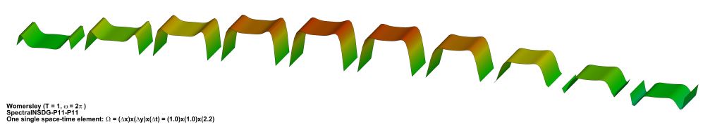
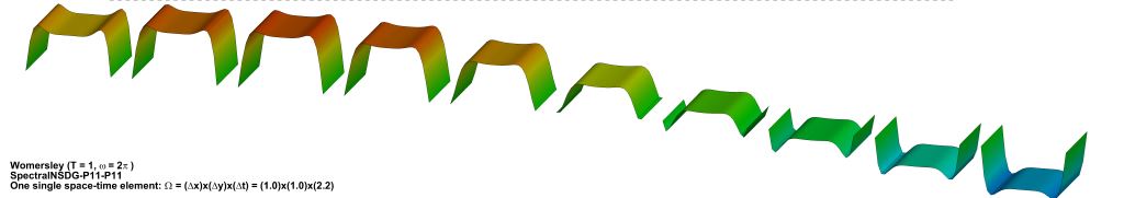
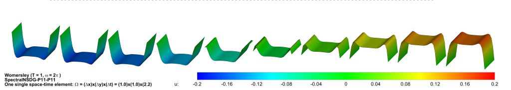
Figure 12: The numerical solution obtained for the two-dimensional oscillatory flow between two flat plates with the staggered spectral space-time DG-$\mathbb{P}_{11}$ scheme. The computational domain in space and time $\Omega=\Delta x\times\Delta y\times\Delta t=1.0\times 1.0\times 2.2$ has been discretized by using only one single space time element, and the plotted numerical solution for the velocity field has been interpolated along $40$ time slices with $t\in[0,2.2]$, respectively, from top left to bottom right.

where $i=\sqrt{-1}$ is the imaginary unit, $L=x_{R}-x_{L}$ is the total length of the duct and the amplitude has been chosen equal to $A=1$. The exact solution has been chosen as initial condition at $t=0$, then pressure conditions are imposed on the left and right boundaries, while no-slip boundary conditions have been imposed at the upper and lower walls. The other parameters of this test problem were chosen as $L=1$, $R=0.5$ and $\omega=1$. Figs. 11 and 12 show the numerical results obtained for $\nu=2\cdot 10^{-2}$ with our spectral staggered space-time DG scheme using only one single $\textnormal{P}_{11}$ space-time element (M=N=11), completing the entire simulation within the time interval $t\in[0,2.2]$ in one single time step. The results are compared with the exact analytical solution at different intermediate output times. In particular, for this test problem, two periods of oscillation are resolved within a single time-step, and the complete velocity profile is resolved within a single spatial cell. From the obtained results one can conclude that the proposed staggered spectral space-time DG scheme is indeed very accurate in both space and time, since it is able to resolve all flow features within one single space-time element.

Furthermore, Table 1 contains the results of a numerical convergence study that we have performed with this smooth unsteady two-dimensional flow problem, for which an exact solution is available. The order of accuracy has been verified up to order $7$ in space and time by evaluating the $L_{2}$ and $L_{\infty}$ errors

$$\epsilon_{L_{2}}=\sqrt{\int_{\Omega}\left(u_{h}-u\right)^{2}},\;\;\;\text{and}\;\;\;\epsilon_{L_{\infty}}=\max\limits_{\Omega}\left|u_{h}-u\right|,$$

at different discretization numbers for the polynomial degrees $N=M=1,\ldots,6$. From the obtained results we conclude that the designed order of accuracy of the scheme has been reached in both space and time. For the polynomial degree $N=M=1$, only sub-optimal convergence rates have been verified experimentally, and will be subject of future research.

3.4.2 2D Taylor-Green vortex

The two dimensional Taylor-Green vortex problem is widely used for testing the accuracy of numerical schemes, because it offers another smooth unsteady analytical solution of the incompressible Navier-Stokes equations with periodic boundary conditions. The exact solution of this problem is given by

$$u(x,y,t)=\sin(x)\cos(y)e^{-2\nu t},\qquad v(x,y,t)=-\cos(x)\sin(y)e^{-2\nu t},$$

$$p(x,y,t)=\frac{1}{4}\left(\cos(2x)+\cos(2y)\right)e^{-4\nu t}.$$

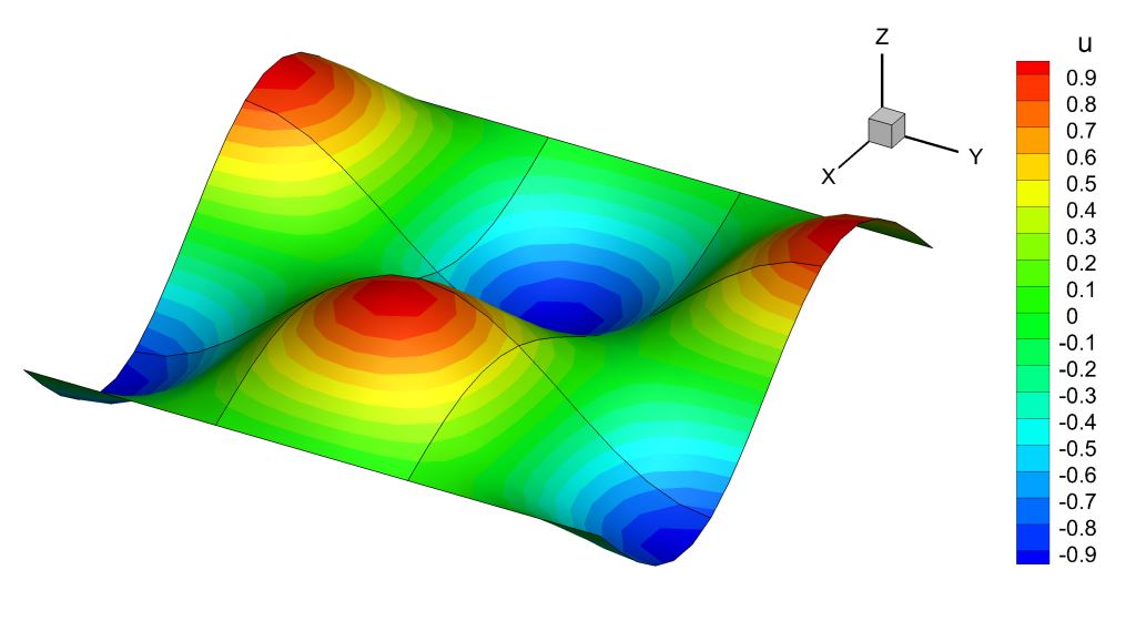
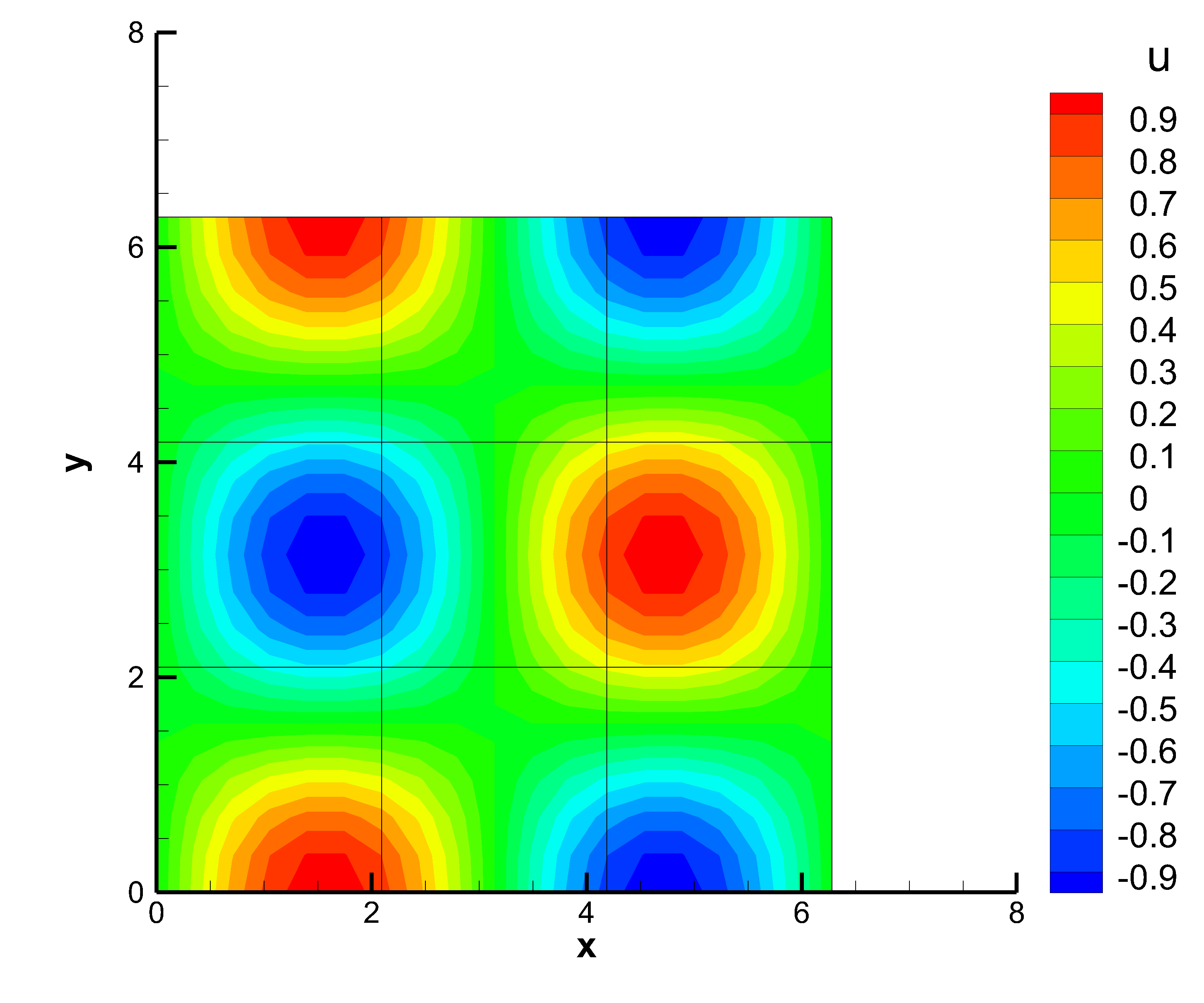
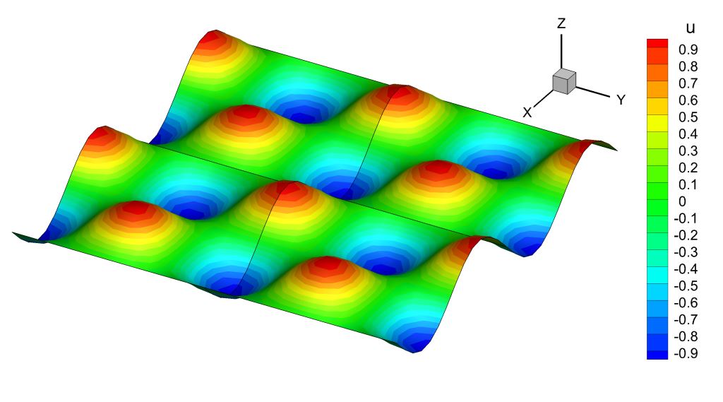
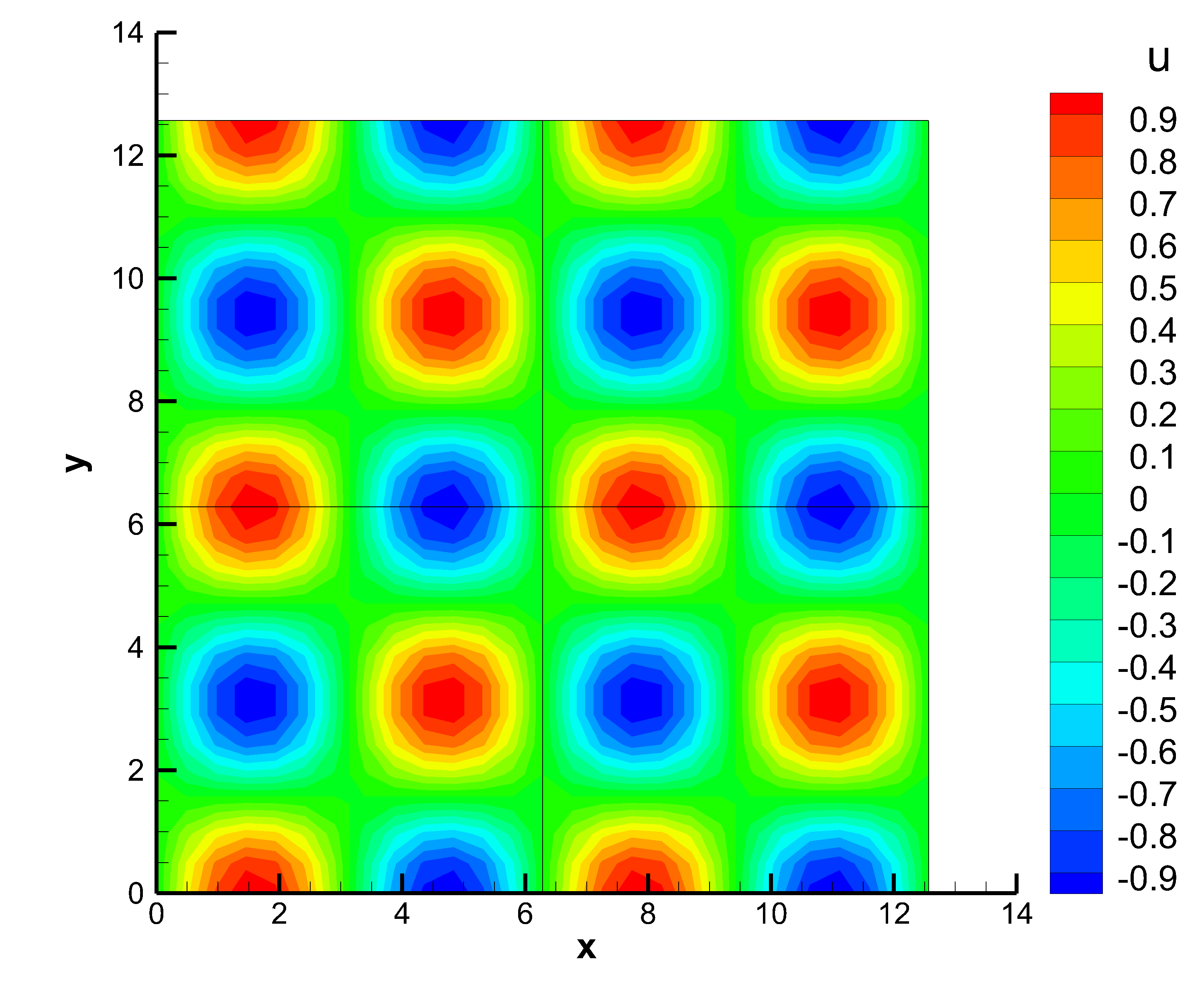
Figure 13: Numerical solution of the $u$ velocity component for the two dimensional Taylor-Green vortex problem computed with the staggered spectral space-time DG-$\mathbb{P}_{5}$ method using $3^{2}$ elements with $L=2\pi$ (top) and the staggered spectral space-time DG-$\mathbb{P}_{12}$ scheme using $2^{2}$ elements with $L=4\pi$ (bottom).

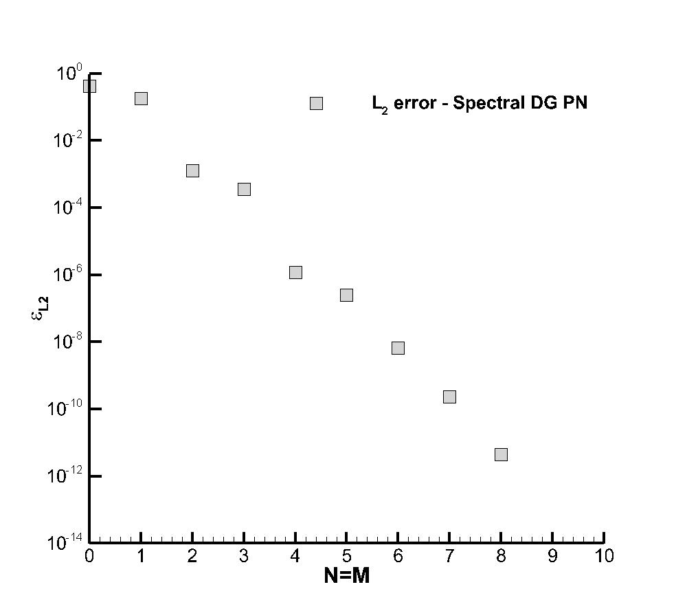
Figure 14: Numerical $L_{2}$ error $\epsilon_{L_{2}}$ of the $u$ velocity component for the two dimensional Taylor-Green vortex problem computed with staggered spectral space-time DG-$\mathbb{P}_{N}$ schemes as a function of the polynomial degree $N=M$ on a fixed grid of $12^{2}$ elements.

The computational domain is $\Omega=[0,L]^{2}$ with periodic boundary conditions. The initial sinusoidal velocity field is smoothed in time by the viscous dissipative forces. The convergence study for this test is summarized in Table 2. The accuracy of our staggered spectral space-time DG scheme is verified for polynomial degrees $N=M=1,\ldots,8$. Figure 13 shows the numerical solution obtained by setting $L=2\pi$ for the staggered spectral space-time DG-$\mathbb{P}_{5}$ scheme, using a very coarse mesh composed of only $3^{2}$ spatial elements. Furthermore, we repeat this test with $L=4\pi$ using a staggered spectral space-time DG-$\mathbb{P}_{12}$ scheme using only $2^{2}$ spatial elements. Moreover, Figure 14 shows the behavior of the error $\epsilon_{L_{2}}$ as a function of the polynomial degree ($N=M$) for a fixed mesh: the exponential decay of the error, i.e. the spectral convergence obtained with our scheme by increasing the polynomial approximation degree in space and time, is explicitly verified. The results confirm the designed accuracy in space and time and show how the presented numerical method works properly even when using very high order approximation polynomials and very coarse meshes. Also in this two dimensional test, for the polynomial degree $N=M=1$ a non-optimal convergence has been experimetally verified.

3.4.3 3D Arnold-Beltrami-Childress flow

In order to test the accuracy of our staggered spectral space-time DG scheme also against an unsteady three dimensional benchmark problem, the Arnold-Beltrami-Childress (ABC) flow, proposed by Arnold [6] and Childress in [40], is considered. For this smooth unsteady test problem, the exact solution reads

$$u(x,y,z,t)=\left[\sin(z)+\cos(y)\right]e^{-\nu t},$$

$$v(x,y,z,t)=\left[\sin(x)+\cos(z)\right]e^{-\nu t},$$ (139)

$$w(x,y,z,t)=\left[\sin(y)+\sin(x)\right]e^{-\nu t}.$$

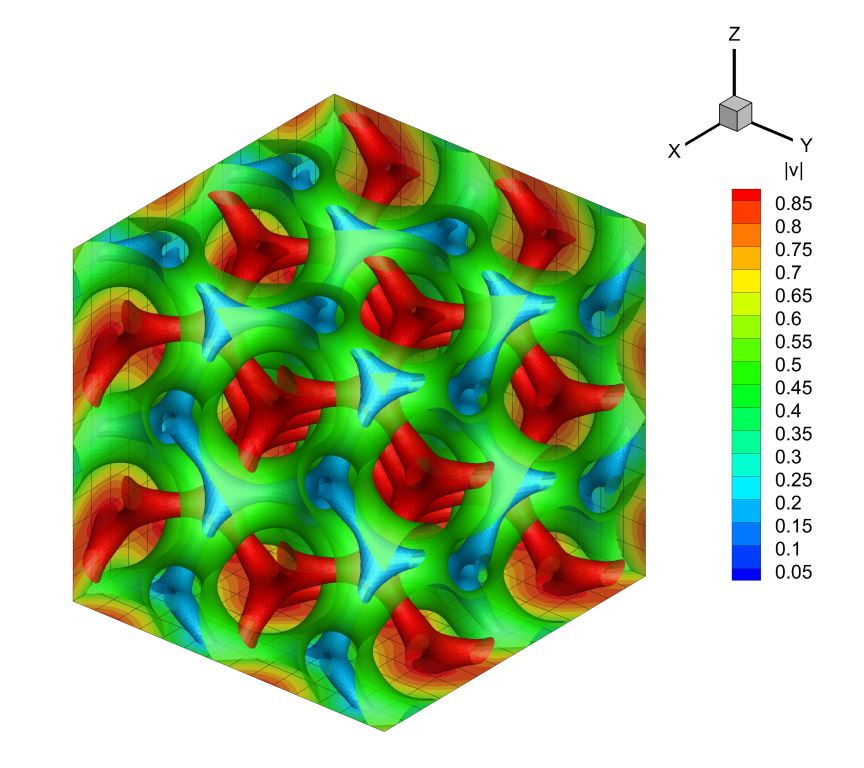
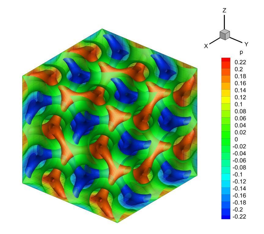
Figure 15: Numerical solution for the three dimensional Arnold-Beltrami-Childress (ABC) flow at time $t=1.0$ computed with the staggered spectral space-time DG-$\mathbb{P}_{5}$ scheme using only $7^{3}$ elements in space. The periodic solution has been replicated along the three dimensional cube of edge $L_{c}=4\pi$ for giving a better view of the field variables. At the top of the figure the velocity is plotted on the left and the pressure is depicted on the right; at the bottom the 3D stream-traces together with the pressure isosurfaces are plotted.

The computational domain is the cube $\Omega=[0,2\pi]^{3}$, with periodic boundary conditions everywhere. Given the initial condition (139) at time $t=0$, the corresponding analytical solution decays exponentially in time according to the chosen kinematic viscosity. Also for this three dimensional time-dependent test problem, the designed high order of accuracy of our staggered spectral space-time DG scheme has been confirmed up to order $9$ by a numerical convergence study that is summarized in Table 3. Similar to the two dimensional Taylor-Green vortex, in the 3D ABC flow the advective terms, the pressure forces and the incompressibility condition are highly coupled. The numerical solution for $\nu=0.1$ at time $t=10$ is depicted in Figure 15.

4 Conclusion

In this paper the new family of staggered spectral semi-implicit DG methods, recently proposed by Dumbser and Casulli in [59] for the shallow water equations on staggered Cartesian grids, has been extended to the incompressible Navier-Stokes equations in two and three space dimensions and to arbitrary high order of accuracy in time, adopting a novel staggered spectral space-time DG formalism. A similar formulation has been recently presented in [125, 126, 127] for unstructured staggered meshes, but there the chosen staggered grid was slightly different, and the use of unstructured meshes did not allow to produce a spectral DG scheme based on simple tensor products of one-dimensional operators. Of course, unstructured meshes as those used in [125, 126, 127] allow to fit very complicate geometries and complex physical boundaries, however, by choosing staggered Cartesian grids, some interesting advantages follow, in particular:

1. Cartesian grids allow the use of tensor-products of the basis and test functions; this means that the weak formulation of the governing equations can be written as a very handy combination of one dimensional integrals over the canonical reference element $\xi\in[0,1]$;

2. this fact significantly minimizes the computational costs and difficulties for evaluating integrals, because the defined matrices are the same for all the elements in the Cartesian framework;

3. by using basis functions that are built from the Lagrange interpolation polynomials passing through the Gauss-Legendre quadrature points, the basis functions are orthogonal and thus the resulting mass matrices are diagonal; this fact reduces significantly the computational cost for a mass-matrix multiplication;

4. in our staggered Cartesian framework, each velocity component is defined on a different staggered dual control volume; consequently, the computation of convective and viscous terms on the main grid by interpolating from the dual grids to the main grid and vice versa is simpler and more natural than a discretization of these terms on the dual grids;

5. the resulting numerical method achieves a spectral convergence property, i.e. the computational error decreases exponentially when increasing the degree of the approximation polynomials in space and time.

The key-role of the proposed mesh-staggering, combined with the adopted semi-implicit or space-time DG time discretization, is to optimize the sparsity pattern of the resulting pressure system. Furthermore, the pressure system is symmetric and only block five-diagonal for the 2D case, or only block seven-diagonal for the 3D case. In addition, we have presented a new way of evaluating the viscous terms in the DG framework, computing the velocity gradient (i.e. the stress tensor) on the staggered dual control volumes, which can be interpreted as the use of a Bassi-Rebay-type lifting operator that accounts for the jumps of the solution in the discrete gradients, but on the dual grid. This allows to compute the viscous terms via an implicit discretization with essentially the same coefficient matrix that is already used in the discrete pressure system, with an additional diagonal term that further enforces the stability of the system. The resulting algorithm is shown to be arbitrary higher order accurate in space and time, robust, stable, and very efficient compared to other classical higher order DG methods for the incompressible Navier-Stokes equations on collocated grids, which either lead to a larger computational stencil or to a larger linear system with more unknowns. These features have been verified against a large set of test cases in two and three space dimensions. The designed space-time accuracy of our method has been verified up to $9$-th order through a series of numerical convergence tests in two and three space dimensions.

For the simulation of turbulent flows, very high spatial and temporal resolution is needed for giving a correct and complete description of the flow physics. With the aim of improving the efficiency of our algorithm further, future work will concern the extension of the present high order staggered DG schemes to space-time adaptive meshes, following the ideas outlined in [142, 65, 61, 144, 143]. By introducing adaptive mesh refinement (AMR) for staggered grids, simulations of turbulent flows should become feasible. Moreover, it is a well known fact that discontinuous Galerkin schemes suffer of spurious oscillations when attempting to resolve shocks, because of Gibbs phenomenon. A novel a posteriori approach of shock capturing for DG schemes, without losing the classical subcell resolution properties of the DG method, has been recently proposed for collocated grids in [66, 144, 143]. The extension of this a posteriori subcell limiter techniques to semi-implicit DG schemes on staggered meshes belongs to future investigations. The possibility of extending the present semi-implicit staggered DG schemes to the context of the compressible Navier-Stokes equations, following the ideas of [92, 110, 91, 105, 60], is also another topic of future research.

Figure 2: Top: Comparison of the reference solution of Blasius with the numerical results at $t=5$ for different axial positions $x=0.25$ and $x=0.50$ obtained with a staggered semi-implicit spectral DG-$\textnormal{P}_{7}$ scheme on a very coarse grid of $18\times 6$ elements. Bottom: numerical solution for the horizontal velocity field computed at time $t=5$; the high-order elements of the main grid are depicted with solid lines; the vertical cuts at $x=0.25$ and $x=0.50$ with dash-dotted lines.

Figure 3: The numerical solution obtained for the two dimensional lid-driven cavity problem compared with the numerical results of [75] at different Reynolds numbers, respectively, from the top to the bottom: Re=$100$, Re=$400$, Re=$1000$ using $5x5$ elements, and Re=$3200$ using $15x15$ elements obtained with a staggered semi-implicit spectral DG-$\textnormal{P}_{6}$ method.

Figure 11: The numerical solution interpolated along 100 equidistant spatial points obtained for the unsteady Womersley problem compared with the exact solution [139, 103] at different times for $\nu=2\cdot 10^{-2}$: $t=1.8$, $1.6$, $2.0$, $1.4$, $2.2$, respectively, from the bottom to the top. A staggered spectral space-time DG-$\mathbb{P}_{11}$ method has been run using only one single space-time element.

2D Womersley problem — Spectral-DG-$\mathbb{P}_{N}$
	$N_{\text{el}}$	$\epsilon_{L^{2}}$	$\epsilon_{L^{\infty}}$	$\mathcal{O}_{L^{2}}$	$\mathcal{O}_{L^{\infty}}$			$N_{\text{el}}$	$\epsilon_{L^{2}}$	$\epsilon_{L^{\infty}}$	$\mathcal{O}_{L^{2}}$	$\mathcal{O}_{L^{\infty}}$
	$N=M=1$				($t_{\text{end}}$ = 0.5)			$N=M=2$
	402	1.6288E-03	3.1562E-03	—	—			202	1.1014E-04	4.7994E-04	—	—
	502	1.3100E-03	2.5073E-03	0.98	1.03			252	5.5799E-05	2.5608E-04	3.05	2.82
	602	1.0947E-03	2.0868E-03	0.98	1.00			302	3.1934E-05	1.5173E-04	3.06	2.87
	702	9.3992E-04	1.7923E-03	0.99	0.99			352	1.9913E-05	9.6986E-05	3.06	2.90
	$N=M=3$							$N=M=4$
	162	2.0842E-05	7.7657E-05	—	—			152	2.9044E-06	1.6983E-05	—	—
	202	8.9568E-06	3.1298E-05	3.78	4.07			202	7.3904E-07	4.9121E-06	4.76	4.31
	242	4.4439E-06	1.6255E-05	3.84	3.60			252	2.3730E-07	1.7422E-06	5.09	4.65
	282	2.4474E-06	9.0529E-06	3.87	3.80			302	9.2319E-08	7.2933E-07	5.18	4.78
	$N=M=5$							$N=M=6$				($t_{\text{end}}$ = 2.2)
	82	4.1408E-06	2.1569E-05	—	—			92	1.7483E-07	1.0630E-06	—	—
	122	7.1268E-07	4.5893E-06	4.34	3.82			102	8.4841E-08	5.1637E-07	6.86	6.85
	162	1.7093E-07	1.2088E-06	4.96	4.64			112	4.3911E-08	2.6415E-07	6.91	7.03
	202	5.0328E-08	3.6841E-07	5.48	5.32			122	2.3925E-08	1.4122E-07	6.98	7.20

Table 1: Numerical convergence table for the two dimensional oscillatory flow between two flat plates computed with staggered spectral space-time DG schemes for $N=M=1,\ldots,6$.

2D Taylor-Green vortex problem $L=2\pi$ — Staggered spectral space-time DG-$\mathbb{P}_{N}$
	$N_{\text{el}}$	$\epsilon_{L^{2}}$	$\epsilon_{L^{\infty}}$	$\mathcal{O}_{L^{2}}$	$\mathcal{O}_{L^{\infty}}$			$N_{\text{el}}$	$\epsilon_{L^{2}}$	$\epsilon_{L^{\infty}}$	$\mathcal{O}_{L^{2}}$	$\mathcal{O}_{L^{\infty}}$
	$N=M=1$							$N=M=2$
	202	6.8094E-02	2.0375E-02	—	—			102	2.9023E-03	1.3592E-03	—	—
	252	5.2703E-02	1.5419E-02	1.15	1.25			152	6.6991E-04	3.2999E-04	3.62	3.49
	302	4.2541E-02	1.2114E-02	1.17	1.32			202	2.1652E-04	9.4734E-05	3.93	4.34
	352	3.5663E-02	1.0062E-02	1.14	1.20			252	9.2092E-05	5.0350E-05	3.83	2.83
	$N=M=3$							$N=M=4$
	162	1.3626E-04	7.8999E-05	—	—			162	1.0519E-06	6.1297E-07	—	—
	202	6.5874E-05	3.7886E-05	3.26	3.29			202	2.7970E-07	1.6271E-07	5.94	5.94
	242	3.6213E-05	2.0085E-05	3.28	3.48			242	9.1334E-08	5.3150E-08	6.14	6.14
	282	2.1887E-05	1.1756E-05	3.27	3.47			282	3.4806E-08	2.0411E-08	6.26	6.21
	$N=M=5$							$N=M=6$
	122	2.9725E-07	2.1057E-07	—	—			122	3.9994E-09	2.4762E-09	—	—
	152	8.4575E-08	6.3046E-08	5.63	5.40			152	9.2671E-10	5.6882E-10	6.55	6.59
	182	2.9174E-08	2.2565E-08	5.84	5.64			182	2.6783E-10	1.7230E-10	6.81	6.55
	212	1.1910E-08	9.4502E-09	5.81	5.65			212	8.9312E-11	6.0292E-11	7.12	6.81
	$N=M=7$							$N=M=8$
	62	1.0586E-08	6.3735E-09	—	—			42	3.4616E-08	2.4849E-08	—	—
	92	4.8791E-10	2.6452E-10	7.59	7.85			62	1.5605E-09	7.1039E-10	7.64	8.77
	122	7.2738E-11	3.8053E-11	6.62	6.74			82	6.1523E-11	3.3955E-11	11.24	10.57
	152	1.2830E-11	7.5665E-12	7.78	7.24			102	5.7787E-12	4.9803E-12	10.60	8.60

Table 2: Numerical convergence table computed for the two dimensional Taylor-Green vortex problem using staggered spectral space-time DG schemes with $N=M=1,\ldots,8$.

3D ABC flow problem — Staggered spectral space-time DG-$\mathbb{P}_{N}$
	$N_{\text{el}}$	$\epsilon_{L^{2}}$	$\epsilon_{L^{\infty}}$	$\mathcal{O}_{L^{2}}$	$\mathcal{O}_{L^{\infty}}$			$N_{\text{el}}$	$\epsilon_{L^{2}}$	$\epsilon_{L^{\infty}}$	$\mathcal{O}_{L^{2}}$	$\mathcal{O}_{L^{\infty}}$
	$N=M=1$							$N=M=2$
	122	8.6905E-02	1.0949E-02	—	—			122	6.9061E-03	1.7183E-03	—	—
	162	4.8615E-02	6.6433E-03	2.02	1.74			152	3.3559E-03	8.2081E-04	3.23	3.31
	202	3.2626E-02	4.7890E-03	1.79	1.47			182	1.7856E-03	4.2641E-04	3.46	3.59
	242	2.3886E-02	3.6992E-03	1.71	1.42			212	1.0316E-03	2.4384E-04	3.56	3.63
	$N=M=3$							$N=M=4$
	42	1.2102E-02	2.3277E-03	—	—			42	1.2102E-02	2.3277E-03	—	—
	62	2.1258E-03	4.9684E-04	4.29	3.81			62	2.1258E-03	4.9684E-04	4.29	3.81
	82	6.4822E-04	1.6790E-04	4.13	3.77			82	6.4822E-04	1.6790E-04	4.13	3.77
	102	2.6346E-04	7.5594E-05	4.03	3.58			102	2.6346E-04	7.5594E-05	4.03	3.58
	$N=M=5$							$N=M=6$
	22	4.6766E-03	9.2223E-04	—	—			22	2.4587E-04	8.9231E-05	—	—
	42	6.6120E-05	1.9076E-05	6.14	5.60			42	4.2976E-06	1.2496E-06	5.84	6.16
	62	5.7711E-06	2.1200E-06	6.01	5.42			62	3.6205E-07	1.0417E-07	6.10	6.13
	82	1.1153E-06	5.0069E-07	5.71	5.02			82	5.6088E-08	1.6526E-08	6.48	6.40
	$N=M=7$							$N=M=8$
	22	5.4083E-05	1.4183E-05	—	—			12	1.5955E-03	5.0110E-04	—	—
	32	2.1818E-06	7.6077E-07	7.92	7.22			22	2.1017E-06	1.0666E-06	9.57	8.88
	42	2.1037E-07	6.2486E-08	8.13	8.69			32	9.7717E-08	3.5484E-08	7.57	8.39
	52	3.5196E-08	1.3221E-08	8.01	6.96			42	1.0666E-08	3.4279E-09	7.70	8.12

Table 3: Numerical convergence table for the three dimensional Arnold-Beltrami-Childress (ABC) flow problem computed with staggered spectral space-time DG schemes for $N=M=1,\ldots,8$.

space	Collocated grid	Vertex-based staggered grid	Edge-based staggered grid
dimensions	(A–grid)	(B–grid)	(C–grid)
1D	$5$	$\mathbf{3}$	$\mathbf{3}$
2D	$9$	$9$	$\mathbf{5}$
3D	$13$	$27$	$\mathbf{7}$

Table 4: Total stencil-size for the resulting pressure systems for semi-implicit DG schemes using different grid types for different numbers of space dimensions. In all cases it is assumed that the discrete momentum equation is substituted into the discrete continuity equation, in order to yield one single equation system for the scalar pressure.

References

• [1] S. Albensoeder and H.C. Kuhlmann. Accurate three-dimensional lid-driven cavity flow. Journal of Computational Physics, 206(2):536 – 558, 2005.
• [2] A. Arakawa and V.R. Lamb. Computational design of the basic dynamical processes of the UCLA general circulation model. Methods of Computational Physics, 17:173–265, 1977.
• [3] B. F. Armaly, F. Durst, J. C. F. Pereira, and B. Schönung. Experimental and theoretical investigation of backward-facing step flow. Journal of Fluid Mechanics, 127:473–496, 2 1983.
• [4] D.N. Arnold, F. Brezzi, B. Cockburn, and L.D. Marini. Unified analysis of discontinuous Galerkin methods for elliptic problems. SIAM J. Numer. Anal., 39(5):1749–1779, May 2001.
• [5] D.N. Arnold, F. Brezzi, and M. Fortin. A stable finite element for the Stokes equations. Calcolo, 21(4):337–344, 1984.
• [6] V.I. Arnold. Sur la topologic des écoulements stationnaires des fluides parfaits. Comptes Rendus Hebdomadaires des Séances de l’Académie des Sciences, 261:17–20, 1965.
• [7] T. Barth and P. Charrier. Energy stable flux formulas for the discontinuous Galerkin discretization of first-order nonlinear conservation laws. Technical Report NAS-01-001, NASA, 2001.
• [8] F. Bassi, A. Crivellini, D.A. Di Pietro, and S. Rebay. An implicit high-order discontinuous Galerkin method for steady and unsteady incompressible flows. Computers & Fluids, 36(10):1529 – 1546, 2007.
• [9] F. Bassi and S. Rebay. A high-order accurate discontinuous finite element method for the numerical solution of the compressible Navier-Stokes equations. Journal of Computational Physics, 131:267–279, 1997.
• [10] C.E. Baumann and J.T. Oden. A discontinuous hp finite element method for convection-diffusion problems. Computer Methods in Applied Mechanics and Engineering, 175:311–341, 1999.
• [11] C.E. Baumann and J.T. Oden. A discontinuous hp finite element method for the Euler and Navier-Stokes equations. International Journal for Numerical Methods in Fluids, 31:79–95, 1999.
• [12] A.D. Beck, T. Bolemann, D. Flad, H. Frank, G.J. Gassner, F. Hindenlang, and C.-D. Munz. High-order discontinuous Galerkin spectral element methods for transitional and turbulent flow simulations. International Journal for Numerical Methods in Fluids, 76:522–548, 2014.
• [13] A. Bermudez, A. Dervieux, J.A. Desideri, and M.E. Vázquez Cendón. Upwind schemes for the two–dimensional shallow water equations with variable depth using unstructured meshes. Computer Methods in Applied Mechanics and Engineering, 155:49–72, 1998.
• [14] A. Bermúdez, J.L. Ferrín, L. Saavedra, and M.E. Vázquez Cendón. A projection hybrid finite volume/element method for low-Mach number flows. Journal of Computational Physics, 271:360–378, 2014.
• [15] W. Boscheri, M. Dumbser, and M. Righetti. A semi-implicit scheme for 3d free surface flows with high order velocity reconstruction on unstructured Voronoi meshes. International Journal for Numerical Methods in Fluids, 72:607– 631, 2013.
• [16] M. E. Brachet, D. I. Meiron, S. A. Orszag, B. G. Nickel, R. H. Morf, and U. Frisch. Small-scale structure of the Taylor-Green vortex. Journal of Fluid Mechanics, 130:411–452, 5 1983.
• [17] F. Brezzi, C. Canuto, and A. Russo. A self-adaptive formulation for the Euler/Navier-Stokes coupling. Computer Methods in Applied Mechanics and Engineering, 73(3):317–330, 1989.
• [18] A. N. Brooks and T. J. R. Hughes. Streamline upwind/Petrov-Galerkin formulations for convection dominated flows with particular emphasis on the incompressible navier-stokes equations. Computer Methods in Applied Mechanics and Engineering, 32(1-3):199 – 259, 1982.
• [19] L. Brugnano and V. Casulli. Iterative solution of piecewise linear systems. SIAM Journal on Scientific Computing, 30:463–472, 2008.
• [20] L. Brugnano and V. Casulli. Iterative solution of piecewise linear systems and applications to flows in porous media. SIAM Journal on Scientific Computing, 31:1858–1873, 2009.
• [21] L. Brugnano and A. Sestini. Iterative solution of piecewise linear systems for the numerical solution of obstacle problems. Journal of Numerical Analysis, Industrial and Applied Mathematics, 6:67–82, 2012.
• [22] C. Canuto, S.I. Hariharan, and L. Lustman. Spectral methods for exterior elliptic problems. Numerische Mathematik, 46(4):505–520, 1985.
• [23] C. Canuto, Y. Maday, and A. Quarteroni. Combined finite element and spectral approximation of the Navier-Stokes equations. Numerische Mathematik, 44(2):201–217, 1984.
• [24] C. Canuto, A. Russo, and V. Van Kemenade. Stabilized spectral methods for the Navier-Stokes equations: Residual-free bubbles and preconditioning. Computer Methods in Applied Mechanics and Engineering, 166(1-2):65–83, 1998.
• [25] C. Canuto and V. Van Kemenade. Bubble-stabilized spectral methods for the incompressible Navier-Stokes equations. Computer Methods in Applied Mechanics and Engineering, 135(1-2):35–61, 1996.
• [26] V. Casulli. Semi-implicit finite difference methods for the two-dimensional shallow water equations. J. Comp. Phys., 86:56–74, 1990.
• [27] V. Casulli. A semi-implicit finite difference method for non-hydrostatic, free-surface flows. Int. J. Numeric. Meth. Fluids, 30:425–440, 1999.
• [28] V. Casulli. A high-resolution wetting and drying algorithm for free-surface hydrodynamics. International Journal for Numerical Methods in Fluids, 60:391–408, 2009.
• [29] V. Casulli. A semi–implicit numerical method for the free–surface Navier–Stokes equations. International Journal for Numerical Methods in Fluids, 74:605–622, 2014.
• [30] V. Casulli and E. Cattani. Stability, accuracy and efficiency of a semi implicit method for three-dimensional shallow water flow. Comp. Math. Appl., 27:99–112, 1994.
• [31] V. Casulli and R. T. Cheng. Semi-implicit finite difference methods for three-dimensional shallow water flow. Int. J. Numeric. Meth. Fluids, 15:629–648, 1992.
• [32] V. Casulli, M. Dumbser, and E.F. Toro. Semi-implicit numerical modeling of axially symmetric flows in compliant arterial systems. Int. J. Numeric. Meth. Biomed. Engng., 28:257–272, 2012.
• [33] V. Casulli and D. Greenspan. Pressure method for the numerical solution of transient, compressible fluid flows. International Journal for Numerical Methods in Fluids, 4(11):1001–1012, 1984.
• [34] V. Casulli and G. S. Stelling. Semi-implicit subgrid modelling of three-dimensional free-surface flows. International Journal for Numerical Methods in Fluids, 67:441–449, 2011.
• [35] V. Casulli and R. A. Walters. An unstructured grid, three-dimensional model based on the shallow water equations. Int. J. Numeric. Meth. Fluids, 32:331–348, 2000.
• [36] V. Casulli and P. Zanolli. Semi-implicit numerical modeling of nonhydrostatic free-surface flows for environmental problems. Math. Comp. Model., 36:1131–1149, 2002.
• [37] V. Casulli and P. Zanolli. A nested newton–type algorithm for finite volume methods solving Richards’ equation in mixed form. SIAM Journal on Scientific Computing, 32:2255–2273, 2009.
• [38] V. Casulli and P. Zanolli. Iterative solutions of mildly nonlinear systems. J. Comp. Appl. Math., 236:3937–3947, 2012.
• [39] S.W. Cheung, E. Chung, H.H. Kim, and Y. Qian. Staggered discontinuous Galerkin methods for the incompressible Navier Stokes equations. Journal of Computational Physics, 302:251–266, 2015.
• [40] S. Childress. New solutions of the kinematic dynamo problem. Journal of Mathematical Physics, 11:3063–3076, 1970.
• [41] A.J. Chorin. A numerical method for solving incompressible viscous flow problems. Journal of Computational Physics, 2(1):12–26, 1967.
• [42] A.J. Chorin. Numerical solution of the Navier-Stokes equations. Mathematics of Computation, 22(104):745–762, 1968.
• [43] E.T. Chung, P. Ciarlet, and T.F. Yu. Convergence and superconvergence of staggered discontinuous Galerkin methods for the three–dimensional Maxwell’s equations on Cartesian grids. Journal of Computational Physics, 235:14–31, 2013.
• [44] E.T. Chung, H.H. Kim, and O.B. Widlund. Two–level overlapping Schwarz algorithms for a staggered discontinuous Galerkin method. SIAM Journal on Numerical Analysis, 51:47–67, 2013.
• [45] E.T. Chung and C.S. Lee. A staggered discontinuous Galerkin method for the convection–diffusion equation. Journal of Numerical Mathematics, 20(1):1–32, 2012.
• [46] B. Cockburn, S. How, and C.-W. Shu. TVB Runge Kutta Local Projection Discontinuous Galerkin Finite Element Method for Conservation Laws IV: The Multidimensional Case. Math. Comp., 54:545, 1990.
• [47] B. Cockburn, G. E. Karniadakis, and C.-W. Shu. Discontinuous Galerkin Methods: Theory, Computation and Applications. Lacture Notes on Computational Science and Engineering. Springer, 2000.
• [48] B. Cockburn, S.-Y. Lin, and C.-W. Shu. TVB Runge Kutta Local Projection Discontinuous Galerkin Finite Element Method for Conservation Laws III: One-Dimensional Systems. Journal of Computational Physics, 84:90, September 1989.
• [49] B. Cockburn and C.-W. Shu. TVB Runge Kutta Local Projection Discontinuous Galerkin Finite Element Method for Scalar Conservation Laws II: General Framework. Math. Comp., 52:411, 1989.
• [50] B. Cockburn and C.W. Shu. The local discontinuous Galerkin method for time-dependent convection-diffusion systems. SIAM Journal on Numerical Analysis, 35(6):2440–2463, 1998.
• [51] B. Cockburn and C.W. Shu. The Runge–Kutta discontinuous Galerkin method for conservation laws V: multidimensional systems. Journal of Computational Physics, 141(2):199–224, 1998.
• [52] B. Cockburn and C.W. Shu. Runge-Kutta discontinuous Galerkin methods for convection-dominated problems. Journal of Scientific Computing, 16(3):173, 2001.
• [53] A. Crivellini, V. D’Alessandro, and F. Bassi. High-order discontinuous Galerkin solutions of three-dimensional incompressible RANS equations. Computers and Fluids, 81:122–133, 2013.
• [54] V. Dolejsi. Semi-implicit interior penalty discontinuous Galerkin method for viscous compressible flows. Communications in Computational Physics, 4(2):231–274, 2008.
• [55] V. Dolejsi and M. Feistauer. A semi-implicit discontinuous Galerkin finite element method for the numerical solution of inviscid compressible flow. Journal of Computational Physics, 198(2):727 – 746, 2004.
• [56] V. Dolejsi, M. Feistauer, and J. Hozman. Analysis of semi-implicit DGFEM for nonlinear convection-diffusion problems on nonconforming meshes. Computer Methods in Applied Mechanics and Engineering, 196(29-30):2813 – 2827, 2007.
• [57] M. Dumbser. Arbitrary high order PNPM schemes on unstructured meshes for the compressible Navier–Stokes equations. Computers & Fluids, 39:60–76, 2010.
• [58] M. Dumbser, D. S. Balsara, E. F. Toro, and C.-D. Munz. A unified framework for the construction of one-step finite volume and discontinuous Galerkin schemes on unstructured meshes. Journal of Computational Physics, 227:8209–8253, September 2008.
• [59] M. Dumbser and V. Casulli. A staggered semi-implicit spectral discontinuous Galerkin scheme for the shallow water equations. Applied Mathematics and Computation, 219(15):8057 – 8077, 2013.
• [60] M. Dumbser and V. Casulli. A conservative, weakly nonlinear semi-implicit finite volume scheme for the compressible Navier–Stokes equations with general equation of state. Applied Mathematics and Computation, 272, Part 2:479 – 497, 2016.
• [61] M. Dumbser, A. Hidalgo, and O. Zanotti. High Order Space-Time Adaptive ADER-WENO Finite Volume Schemes for Non-Conservative Hyperbolic Systems. Computer Methods in Applied Mechanics and Engineering, 268:359–387, 2014.
• [62] M. Dumbser, U. Iben, and M. Ioriatti. An efficient semi-implicit finite volume method for axially symmetric compressible flows in compliant tubes. Applied Numerical Mathematics, 89:24 – 44, 2015.
• [63] M. Dumbser and C.D. Munz. Building blocks for arbitrary high order discontinuous Galerkin schemes. Journal of Scientific Computing, 27:215–230, 2006.
• [64] M. Dumbser, I. Peshkov, and E. Romenski. High order ADER schemes for a unified first order hyperbolic formulation of continuum mechanics: Viscous heat-conducting fluids and elastic solids. Journal of Computational Physics, 314:824–862, 2016.
• [65] M. Dumbser, O. Zanotti, A. Hidalgo, and D.S. Balsara. ADER-WENO Finite Volume Schemes with Space-Time Adaptive Mesh Refinement. Journal of Computational Physics, 248:257–286, 2013.
• [66] M. Dumbser, O. Zanotti, R. Loubère, and S. Diot. A posteriori subcell limiting of the discontinuous Galerkin finite element method for hyperbolic conservation laws. Journal of Computational Physics, 278:47–75, 2014.
• [67] E. Erturk. Numerical solutions of 2-d steady incompressible flow over a backward-facing step, part i: High reynolds number solutions. Computers and Fluids, 37(6):633 – 655, 2008.
• [68] F. Fambri, M. Dumbser, and V. Casulli. An efficient semi-implicit method for three-dimensional non-hydrostatic flows in compliant arterial vessels. International Journal for Numerical Methods in Biomedical Engineering, 30(11):1170–1198, 2014.
• [69] M. Fortin. Old and new finite elements for incompressible flows. International Journal for Numerical Methods in Fluids, 1(4):347–364, 1981.
• [70] G. Gassner and D.A. Kopriva. A comparison of the dispersion and dissipation errors of Gauss and Gauss-Lobatto discontinuous Galerkin spectral element methods. SIAM Journal on Scientific Computing, 33(5):2560–2579, 2011.
• [71] G. Gassner, F. Lörcher, and C. D. Munz. A discontinuous Galerkin scheme based on a space-time expansion II. viscous flow equations in multi dimensions. Journal of Scientific Computing, 34:260–286, 2008.
• [72] G. Gassner, F. Lörcher, and C.D. Munz. A contribution to the construction of diffusion fluxes for finite volume and discontinuous Galerkin schemes. Journal of Computational Physics, 224:1049–1063, 2007.
• [73] G.J. Gassner. A skew-symmetric discontinuous Galerkin spectral element discretization and its relation to sbp-sat finite difference methods. SIAM Journal on Scientific Computing, 35(3):A1233–A1253, 2013.
• [74] G.J. Gassner, A.R. Winters, and D.A. Kopriva. A well balanced and entropy conservative discontinuous Galerkin spectral element method for the shallow water equations. Applied Mathematics and Computation, 272:291–308, 2016.
• [75] U. Ghia, K.N. Ghia, and C.T. Shin. High-Re solutions for incompressible flow using the Navier-Stokes equations and a multigrid method. Journal of Computational Physics, 48(3):387 – 411, 1982.
• [76] F. X. Giraldo and M. Restelli. High-order semi-implicit time-integrators for a triangular discontinuous Galerkin oceanic shallow water model. International Journal for Numerical Methods in Fluids, 63(9):1077–1102, 2010.
• [77] U. Grenander and G. Szegö. Toeplitz Forms and Their Applications, volume 321. Second Edition, Chelsea, New York, 1984.
• [78] F. H. Harlow and J. E. Welch. Numerical calculation of time‐dependent viscous incompressible flow of fluid with free surface. Physics of Fluids, 8(12):2182–2189, 1965.
• [79] R. Hartmann and P. Houston. Symmetric interior penalty DG methods for the compressible Navier–Stokes equations I: Method formulation. Int. J. Num. Anal. Model., 3:1–20, 2006.
• [80] R. Hartmann and P. Houston. An optimal order interior penalty discontinuous Galerkin discretization of the compressible Navier–Stokes equations. Journal of Computational Physics, 227:9670–9685, 2008.
• [81] J.G. Heywood and R. Rannacher. Finite element approximation of the nonstationary Navier-Stokes problem. I. regularity of solutions and second-order error estimates for spatial discretization. SIAM Journal on Numerical Analysis, 19(2):275–311, 1982.
• [82] J.G. Heywood and R. Rannacher. Finite element approximation of the nonstationary Navier-Stokes problem III. smoothing property and higher order error estimates for spatial discretization. SIAM Journal on Numerical Analysis, 25(3):489–512, 1988.
• [83] A. Hidalgo and M. Dumbser. ADER schemes for nonlinear systems of stiff advection diffusion reaction equations. Journal of Scientific Computing, 48:173–189, 2011.
• [84] S. Hou and X. D. Liu. Solutions of multi-dimensional hyperbolic systems of conservation laws by square entropy condition satisfying discontinuous Galerkin method. Journal of Scientific Computing, 31:127–151, 2007.
• [85] T. J.R. Hughes, M. Mallet, and M. Akira. A new finite element formulation for computational fluid dynamics: II. Beyond SUPG. Computer Methods in Applied Mechanics and Engineering, 54(3):341 – 355, 1986.
• [86] G. S. Jiang and C.-W. Shu. On a cell entropy inequality for discontinuous Galerkin methods. Mathematics of Computation, 62:531–538, 1994.
• [87] G. E. Karniadakis, M. Israeli, and S. A. Orszag. High-order splitting methods for the incompressible Navier-Stokes equations. Journal of Computational Physics, 97(2):414 – 443, 1991.
• [88] J. Kim and P. Moin. Application of a fractional-step method to incompressible Navier–Stokes equations. Journal of Computational Physics, 59(2):308 – 323, 1985.
• [89] C. Klaij, J.J.W. Van der Vegt, and H. Van der Ven. Space-time discontinuous Galerkin method for the compressible Navier-Stokes equations. Journal of Computational Physics, 217:589–611, 2006.
• [90] B. Klein, F. Kummer, and M. Oberlack. A SIMPLE based discontinuous Galerkin solver for steady incompressible flows. Journal of Computational Physics, 237:235–250, 2013.
• [91] R. Klein. Semi-implicit extension of a godunov-type scheme based on low mach number asymptotics I: one-dimensional flow. Journal of Computational Physics, 121:213–237, 1995.
• [92] R. Klein, N. Botta, T. Schneider, C.D. Munz, S.Roller, A. Meister, L. Hoffmann, and T. Sonar. Asymptotic adaptive methods for multi-scale problems in fluid mechanics. J. of Eng. Math., 39:261–343, 2001.
• [93] D.A. Kopriva. Metric identities and the discontinuous spectral element method on curvilinear meshes. Journal of Scientific Computing, 26(3):301–327, 2006.
• [94] D.A. Kopriva and G. Gassner. On the quadrature and weak form choices in collocation type discontinuous Galerkin spectral element methods. Journal of Scientific Computing, 44(2):136–155, 2010.
• [95] H. C. Ku, R. S. Hirsh, and T. D. Taylor. A pseudospectral method for solution of the three-dimensional incompressible Navier-Stokes equations. Journal of Computational Physics, 70(2):439 – 462, 1987.
• [96] U. H. Kurzweg. Enhanced heat conduction in oscillating viscous flows within parallel-plate channels. Journal of Fluid Mechanics, 156:291–300, 7 1985.
• [97] L. D. Landau and E. M. Lifshitz. Fluid Mechanics, Course of Theoretical Physics, Volume 6. Elsevier Butterworth-Heinemann, Oxford, 2004.
• [98] A.T. Layton. On the choice of correctors for semi-implicit Picard deferred correction methods. Applied Numerical Mathematics, 58(6):845–858, 2008.
• [99] T. Lee and D. Mateescu. Experimental and numerical investigation of 2-d backward-facing step flow. Journal of Fluids and Structures, 12(6):703 – 716, 1998.
• [100] D. Levy, C.W. Shu, and J. Yan. Local discontinuous Galerkin methods for nonlinear dispersive equations. Journal of Computational Physics, 196(2):751–772, 2004.
• [101] C. Liu, C.W. Shu, E. Tadmor, and M. Zhang. L2 stability analysis of the central discontinuous galerkin method and a comparison between the central and regular discontinuous galerkin methods. ESAIM: Mathematical Modelling and Numerical Analysis, 42(04):593–607, 2008.
• [102] Y. Liu, C.W. Shu, E. Tadmor, and M. Zhang. Central discontinuous Galerkin methods on overlapping cells with a nonoscillatory hierarchical reconstruction. SIAM Journal on Numerical Analysis, 45(6):2442–2467, 2007.
• [103] C. Loudon and A. Tordesillas. The use of the dimensionless womersley number to characterize the unsteady nature of internal flow. Journal of Theoretical Biology, 191(1):63 – 78, 1998.
• [104] Philip S. Marcus. Simulation of taylor-couette flow. part 1. numerical methods and comparison with experiment. Journal of Fluid Mechanics, 146:45–64, 9 1984.
• [105] A. Meister. Asymptotic single and multiple scale expansions in the low mach number limit. SIAM Journal on Applied Mathematics, 60(1):256–271, 1999.
• [106] M. L. Minion. Semi-implicit spectral deferred correction methods for ordinary differential equations. Commun. Math. Sci., 1(3):471–500, 2003.
• [107] M. L. Minion. Higher-order semi-implicit projection methods. in M. Hafez, editor, Numerical Simulations of Incompressible Flows: Proceedings of a Conference Held at Half Moon Bay, CA (June 18-20, 2001), January 2003.
• [108] R. H. Morf, S. A. Orszag, and U. Frisch. Spontaneous singularity in three-dimensional inviscid, incompressible flow. Phys. Rev. Lett., 44:572–575, Mar 1980.
• [109] A.A. Mouza, M.N. Pantzali, S.V. Paras, and J. Tihon. Experimental and numerical study of backward-facing step flow. 5th National Chemical Engineering Conference, Thessaloniki, Greece, 2005.
• [110] C.D. Munz, R. Klein, S. Roller, and K.J. Geratz. The extension of incompressible flow solvers to the weakly compressible regime. Computers and Fluids, pages 173–196, 2003.
• [111] S. V. Patankar and D. B. Spalding. A calculation procedure for heat, mass and momentum transfer in three-dimensional parabolic flows. International Journal of Heat and Mass Transfer, 15(10):1787 – 1806, 1972.
• [112] V.S. Patankar. Numerical Heat Transfer and Fluid Flow. series in computational methods in mechanics and thermal sciences. Hemisphere Publishing Corporation, 1980.
• [113] I. Peshkov and E. Romenski. A hyperbolic model for viscous Newtonian flows. Continuum Mechanics and Thermodynamics, 28:85–104, 2016.
• [114] L. Prandtl. Über Flüssigkeitsbewegung bei sehr kleiner Reibung. Verhandlg. III. Intern. Math. Kongr. Heidelberg, pages 484–491, 1904.
• [115] J. Qiu, M. Dumbser, and C.W. Shu. The discontinuous Galerkin method with Lax-Wendroff type time discretizations. Computer Methods in Applied Mechanics and Engineering, 194:4528–4543, 2005.
• [116] H. P. Rani, Tony W. H. Sheu, and Eric S. F. Tsai. Eddy structures in a transitional backward-facing step flow. Journal of Fluid Mechanics, 588:43–58, 10 2007.
• [117] W. H Reed and T. R. Hill. Triangular mesh methods for the neutron transport equation. Technical report, Los Alamos Scientific Laboratory, 1973.
• [118] V. V. Rusanov. Calculation of Interaction of Non–Steady Shock Waves with Obstacles. J. Comput. Math. Phys. USSR, 1:267–279, 1961.
• [119] Y. Saad and M. H. Schultz. GMRES: A generalized minimum residual algorithm for solving nonsymmetric linear systems. SIAM J. Sci. Stat. Comput., 7(3):856–869, 1986.
• [120] H. Schlichting and K. Gersten. Grenzschichttheorie. Springer Verlag, 2005.
• [121] S. Serra-Capizzano. Asymptotic results on the spectra of block Toeplitz preconditioned matrices. SIAM journal on matrix analysis and applications, 20(1):31–44, 1998.
• [122] S Serra-Capizzano. Generalized locally Toeplitz sequences: spectral analysis and applications to discretized partial differential equations. Linear Algebra Appl., 366:371–402, 2003.
• [123] C. W. Shu and S. J. Osher. Efficient implementation of essentially non-oscillatory shock-capturing schemes. J. Comput. Phys., 77:439, 1988.
• [124] A. Taube, M. Dumbser, D. Balsara, and C.D. Munz. Arbitrary high order discontinuous Galerkin schemes for the magnetohydrodynamic equations. Journal of Scientific Computing, 30:441–464, 2007.
• [125] M. Tavelli and M. Dumbser. A high order semi-implicit discontinuous Galerkin method for the two dimensional shallow water equations on staggered unstructured meshes. Applied Mathematics and Computation, 234:623 – 644, 2014.
• [126] M. Tavelli and M. Dumbser. A staggered semi-implicit discontinuous Galerkin method for the two dimensional incompressible Navier-Stokes equations. Applied Mathematics and Computation, 248:70 – 92, 2014.
• [127] M. Tavelli and M. Dumbser. A staggered space-time discontinuous Galerkin method for the incompressible Navier-Stokes equations on two-dimensional triangular meshes. Computers & Fluids, 119:235 – 249, 2015.
• [128] M. Tavelli and M. Dumbser. A staggered space-time discontinuous Galerkin method for the three-dimensional incompressible Navier-Stokes equations on unstructured tetrahedral meshes. Journal of Computational Physics, 319:294 – 323, 2016.
• [129] C. Taylor and P. Hood. A numerical solution of the Navier–Stokes equations using the finite element technique. Computers & Fluids, 1(1):73 – 100, 1973.
• [130] E. F. Toro. Riemann Solvers and Numerical Methods for Fluid Dynamics. Springer-Verlag, 1999.
• [131] E.F. Toro, A. Hidalgo, and M. Dumbser. FORCE schemes on unstructured meshes I: Conservative hyperbolic systems. Journal of Computational Physics, 228:3368–3389, 2009.
• [132] G. Tumolo, L. Bonaventura, and M. Restelli. A semi-implicit, semi-lagrangian, p-adaptive discontinuous galerkin method for the shallow water equations. Journal of Computational Physics, 232(1):46 – 67, 2013.
• [133] N. Tylli, L. Kaiktsis, and B. Ineichen. Sidewall effects in flow over a backward-facing step: Experiments and numerical simulations. Physics of Fluids, 14(11):3835–3845, 2002.
• [134] E. Tyrtyshnikov and N. Zamarashkin. Spectra of multilevel toeplitz matrices: advanced theory via simple matrix relationships. Linear Algebra Appl., 270:15–27, 1998.
• [135] J. J. W. van der Vegt and H. van der Ven. Space–time discontinuous Galerkin finite element method with dynamic grid motion for inviscid compressible flows I. general formulation. Journal of Computational Physics, 182:546–585, 2002.
• [136] H. van der Ven and J. J. W. van der Vegt. Space–time discontinuous Galerkin finite element method with dynamic grid motion for inviscid compressible flows II. efficient flux quadrature. Comput. Methods Appl. Mech. Engrg., 191:4747–4780, 2002.
• [137] J van Kan. A second-order accurate pressure correction scheme for viscous incompressible flow. SIAM J. Sci. Stat. Comput., 7(3):870–891, July 1986.
• [138] R. Verfürth. Finite element approximation of incompressible Navier-Stokes equations with slip boundary condition II. Numerische Mathematik, 59:615–636, 1991.
• [139] J. R. Womersley. Method for the calculation of velocity, rate of flow and viscous drag in arteries when the pressure gradient is known. The Journal of Physiology, 127(3):553–563, 1955.
• [140] J. Yan and C.W. Shu. A local discontinuous Galerkin method for KdV type equations. SIAM Journal on Numerical Analysis, 40(2):769–791, 2002.
• [141] T. A. Zang and M. Y. Hussaini. On spectral multigrid methods for the time-dependent Navier–Stokes equations. Applied Mathematics and Computation, 19(1-4):359 – 372, 1986.
• [142] O. Zanotti and M. Dumbser. A high order special relativistic hydrodynamic and magnetohydrodynamic code with space-time adaptive mesh refinement. Computer Physics Communications, 188:110–127, 2015.
• [143] O. Zanotti, F. Fambri, and M. Dumbser. Solving the relativistic magnetohydrodynamics equations with ADER discontinuous Galerkin methods, a posteriori subcell limiting and adaptive mesh refinement. Mon. Not. R. Astron. Soc., 452:3010–3029, September 2015.
• [144] O. Zanotti, F. Fambri, M. Dumbser, and A. Hidalgo. Space-time adaptive ADER discontinuous Galerkin finite element schemes with a posteriori sub-cell finite volume limiting. Computers and Fluids, 118:204 – 224, 2015.
Refer to caption Refer to caption