Accretion onto Some Well-Known Regular Black Holes

Abstract

In this work, we discuss the accretion onto static spherical symmetric regular black holes for specific choices of equation of state parameter. The underlying regular black holes are charged regular black hole using Fermi-Dirac Distribution, logistic distribution, nonlinear electrodynamics, respectively and Kehagias-Sftesos asymptotically flat regular black hole. We obtain the critical radius, critical speed and squared sound speed during the accretion process near the regular black holes. We also study the behavior of radial velocity, energy density and rate of change of mass for each regular black holes.

1 Introduction

At present, type 1a supernova [1], Cosmic microwave background (CMB) radiation [2] and large scale structure [3, 4] have shown that our universe is currently in accelerating expansion period. Dark energy is responsible for this acceleration and it has strange property that violates the null energy condition (NEC) and weak energy condition (WEC) [5, 6] and produces strong repulsive gravitational effects. Recent observations suggests that approximately 74% of our universe is occupied by dark energy and the rest 22% and 4% is of dark matter and ordinary matter respectively. Nowadays dark energy is the most challenging problem in astrophysics. Many theories have been proposed to handle this important problem in last two decade. Dark energy is modeled using the relationship between energy density and pressure by perfect fluid with equation of state (EoS) $\rho=\omega p$. The candidates of dark energy are phantom like fluid $(\omega<-1)$, quintessence $(-1<\omega<-1/3)$, cosmological constant $(\omega=-1)$[7]. Other models are also proposed for explanation of dark energy like k-essence, DBI-essence, Hessence, dilation, tachyon, chaplygin gas etc [8]-[16].

On the other hand, existence of essential singularities (which leads to various black holes (BHs)) is one of the major problems in general relativity (GR) and it seems to be a common property in most of the solutions of Einstein field equations. To avoid these singularities, regular BHs (RBHs) have been developed. These BHs are solutions of Einstein Equation with no essential singularity hence their metric is regular everywhere. Strong energy condition (SEC) is violated by these RBHs somewhere in space time [17, 18] while some of these satisfy the WEC. However, it is necessary for those RBHs to satisfy WEC having de sitter center. The study of RBHs solutions is very important to understand the gravitational collapse. Since Penrose cosmic censorship conjecture claims that is singularities predicted by GR [19, 20] occur, they must be explained by event horizons. Bardeen [21] has done a poineer work in this way by presenting the first RBH known as ”Bardeen Black Hole”, which satisfy the WEC.

The discussion about the properties of BHs have led many interesting phenomenon. Accretion onto the BHs is one of them. When a massive condensed object (e.g. black holes, neutron stars, stars etc.) try to capture a particle of the fluid from its surroundings, then the mass of condensed object has been effected. This process is known as accretion of fluid by condensed object. Due to accretion the planets and star form inhomogeneous regions of dust and gas. Supermassive BHs exist at center of giant galaxies which suggests that they could have formed through accretion process. It is not necessary that the mass of BH increases due to accretion process, sometimes in falling matter is thrown away like cosmic rays [22]. First of all, the problem of accretion on compact object was investigated by Bondi using Newtonian theory of gravity [23]. After that many researchers such as Michel [24], Babichev et al. [25, 26], Jamil [27] and Debnath [31] have discussed the accretion on Schwarzschild BH under different aspects. Kim et al [29] and Madrid et al. [30] studied accretion of dark energy on static BH and Kerr-Newman BH. Sharif and Abbas [28] discussed the accretion on stringy charged BHs due to phantom energy.

Recently, framework of accretion on general static spherical symmetric BHs has been presented by Bahamonde and Jamil [22]. We have extended this general formalism for some RBHs. We analyze the effect of mass of RBH by choosing different values of EoS parameter. This paper is established as follows: In section 2, we derive general formalism for spherically static accretion process. In section 3, we discuss some RBHs and for each case, we explain the critical radius, critical points, speed of sound, radial velocities profile, energy density and rate of change of BH mass. In the end, we conclude our results.

2 General Formalism For Accretion

The generalized static spherical symmetry is characterized by the following line element

$$ds^{2}=-X(r)dt^{2}+\frac{1}{Y(r)}dr^{2}+Z(r)(d\theta^{2}+\sin\theta^{2}d\phi^{2}),$$ (1)

where $X(r)>0$, $Y(r)>0$ and $Z(r)>0$ are the functions of $r$ only. The energy-momentum tensor is considered as perfect fluid which is isotropic and inhomogeneous and defined as follows

$$T_{\mu\nu}=(\rho+p)u_{\mu}u_{\nu}+pg_{\mu\nu},$$ (2)

where p is pressure, $\rho$ is energy density and $u^{\mu}$ is the four velocity which is given by

$$u^{\mu}=\frac{dx^{\mu}}{d\tau}=(u^{t},u^{r},0,0),$$ (3)

where $\tau$ is the proper time. We have $u^{\theta}$ and $u^{\phi}$ both equal to zero due to spherical symmetry restrictions. Here pressure, energy density and four velocity components are only the functions of $r$. The normalization condition of four velocity must satisfy $u^{\mu}u_{\mu}=-1$, we get

$$u^{t}:=\frac{dt}{d\tau}=\sqrt{\frac{u^{2}+Y}{XY}},$$ (4)

where $u=dr/d\tau=u^{r}$[22], $u^{t}$ can be negative or positive due to square root which represents the backward or forward in time conditions. However, $u<0$ is required for accretion process otherwise for any outward flows $u>0$. Both inward and outward flows are very important in astrophysics. One can assume that the fluid is dark energy or any kind of dark matter. For spherical symmetric BH, the proper dark energy model could be obtained by generalizing Michel’s theory. In dark energy accretion, Babichev et al. [25] have introduced the above generalization on Schwarzschild black hole. Similarly, some authors [22, 31] have extended this procedure for generalized static spherically symmetric BH. In these works, equation of continuity plays an important role which turns out to be

$$(\rho+p)u\frac{X(r)}{Y(r)}\sqrt{u^{2}+Y(r)}Z(r)=A_{0},$$ (5)

where $A_{0}$ is the constant of integration. Using $u_{\mu}T^{\mu\nu}_{\mu}=0$, we obtain continuity (or relativistic energy flux) equation

$$u^{\mu}\rho_{,\mu}+(\rho+p)u^{\mu}_{;\mu}=0.$$ (6)

Furthermore, assuming $p=p(\rho)$ a certain EoS in this case. After some calculations, the above equation becomes

$$\frac{\rho^{{}^{\prime}}}{\rho+p}+\frac{u^{{}^{\prime}}}{u}+\frac{X^{{}^{\prime}}}{2X}+\frac{Y^{{}^{\prime}}}{2Y}+\frac{Z^{{}^{\prime}}}{Z}=0,$$ (7)

here prime represents the derivative with respect to $r$. By integrating the last equation, we obtain

$$uZ(r)\sqrt{\frac{X(r)}{Y(r)}}e^{\int{\frac{d\rho}{\rho+p(\rho)}}}=-A_{1},$$ (8)

where $A_{1}$ is the constant of integration. By equating Eqs.(5) and (8), we get

$$(\rho+p)\sqrt{\frac{X(r)}{Y(r)}}\sqrt{u^{2}+Y}e^{-\int{\frac{d\rho}{\rho+p(\rho)}}}=-\frac{A_{0}}{A_{1}}=A_{3},$$ (9)

where $A_{3}$ is another constant depends upon $A_{0}$ and $A_{1}$. Moreover, the equation of mass flux yields

$$\rho u\sqrt{\frac{X(r)}{Y(r)}}Z(r)=A_{2},$$ (10)

where $A_{2}$ is the constant of integration. By using Eqs.(5) and (10), we obtain the following important relation

$$\frac{(\rho+p)}{\rho}\sqrt{\frac{X(r)}{Y(r)}}\sqrt{u^{2}+Y}=\frac{A_{1}}{A_{2}}\equiv A_{4},$$ (11)

where $A_{4}$ is arbitrary constant which depends on $A_{1}$ and $A_{2}$. Differentials of Eqs.(10) and (11) and some manipulation leads to

$$\left(V^{2}-\frac{u^{2}}{u^{2}+Y}\right)\frac{du}{u}+\left(\left(V^{2}-1\right)\left(\frac{X^{{}^{\prime}}}{X}-\frac{Y^{{}^{\prime}}}{Y}\right)+\frac{Z^{{}^{\prime}}}{Z}V^{2}-\frac{Y^{{}^{\prime}}}{2\left(u^{2}+Y\right)}\right)dr=0.$$ (12)

In addition, we have introduced the variable

$$V^{2}\equiv\frac{d\ln{\rho+p}}{d\ln{\rho}}-1.$$ (13)

If the bracketed terms in Eq.(12) vanishes, we obtain the critical point (where speed of sound equal to speed of flow) which is located at $r=r_{c}$. Hence at critical point, we get

$$V_{c}^{2}=\frac{u_{c}^{2}}{u_{c}^{2}+Y(r_{c})},$$ (14)

and Eq.(12) turns out to be

$$\left(V^{2}_{c}-1\right)\left(\frac{X^{{}^{\prime}}(r_{c})}{X(r_{c})}-\frac{Y^{{}^{\prime}}(r_{c})}{Y(r_{c})}\right)+\frac{Z^{{}^{\prime}}(r_{c})}{Z(r_{c})}V^{2}_{c}=\frac{Y^{{}^{\prime}}(r_{c})}{2\left(u^{2}_{c}+Y(r_{c})\right)}.$$ (15)

Also, $u_{c}$ is the critical speed of flow evaluated at critical value $r=r_{c}$. We can decoupled the above two equations and obtain

$$u^{2}_{c}=\frac{Y(r_{c})Z(r_{c})X^{{}^{\prime}}(r_{c})}{2X(r_{c})Z^{{}^{\prime}}(r_{c})},\quad V^{2}_{c}=\frac{Z(r_{c})X^{{}^{\prime}}(r_{c})}{2X(r_{c})Z^{{}^{\prime}}(r_{c})+Z(r_{c})X^{{}^{\prime}}(r_{c})}.$$ (16)

The speed of sound is evaluated at $r=r_{c}$ as follows

$$c^{2}_{s}=\frac{dp}{d\rho}|_{r=r_{c}}=A_{4}\sqrt{\frac{Y(r_{c})}{X(r_{c})(u^{2}_{c}+Y(r_{c}))}}-1,$$ (17)

Obviously, $u^{2}_{c}$ and $V^{2}_{c}$ can never be negative and hence

$$\frac{X^{{}^{\prime}}(r_{c})}{Z^{{}^{\prime}}(r_{c})}>0,$$ (18)

Moreover, the rate of change of BH mass can be defined as follows [31]

$$\dot{M}_{acc}=4\pi A_{3}M^{2}(\rho+p),$$ (19)

Here dot is derivative with respect to time. We can observe that the mass of BH will increase for the fluid $\rho+p>0$ and hence the accretion occurs outside the BH. Otherwise, for $\rho+p<0$ like fluid, the mass of BH will decrease. The mass of BH cannot remain fixed because it will decrease in hawking radiation while it will increase in accretion. If we consider the time dependence of BH mass, then first assume that it will not change the geometry and symmetry of space time. Hence the space time metric remain static spherical symmetric [22].

3 Spherical Symmetric Metrics with Charged RBHs

In this section, we discuss the spherically symmetric metrics with charged RBHs in which $X(r)=Y(r)$. For this assumption, Equation (16) give

$$u^{2}_{c}=\frac{Z(r_{c})X^{{}^{\prime}}(r_{c})}{2Z^{{}^{\prime}}(r_{c})},\quad V^{2}_{c}=\frac{Z(r_{c})X^{{}^{\prime}}(r_{c})}{2X(r_{c})Z^{{}^{\prime}}(r_{c})+Z(r_{c})X^{{}^{\prime}}(r_{c})}.$$ (20)

Although, our focus on charged RBHs metrics with event horizons, the present analysis is forbidden for horizon space time. In many cases, we concern on critical values (critical radius), critical velocities, speed of sound in fluid, behavior of energy density of fluid, radial velocity and rate of change of mass of accreting objects. So horizon does not involve anywhere [22].

3.1 Charged RBH Using Fermi-Dirac Distribution

The said RBH solution has the following metric functions [32]

$$X(r)=1-\frac{2M}{r}\left(\frac{\xi(x)(\beta r)}{\xi_{\infty}}\right)^{\beta}=Y(r),$$ (21)

where the Fermi-Dirac distribution function is

$$\xi(x)=\frac{1}{e^{x}+1}.$$ (22)

By replacing $x=\frac{q^{2}}{M\beta r}$, we can obtain the distribution function as

$$\xi(\beta r)=\frac{1}{e^{\frac{q^{2}}{M\beta r}}+1},$$ (23)

with normalization factor is $\xi_{\infty}=\frac{1}{2}$. Also the distribution function satisfies

$$\frac{\xi(r)}{\xi_{\infty}}\rightarrow 1,$$ (24)

where $r\rightarrow\infty$. Hence the metric functions turn out to be

$$X(r)=Y(r)=1-\frac{2M}{r}\left(\frac{2}{e^{\frac{q^{2}}{Mr}}+1}\right)^{\beta},Z(r)=r^{2}.$$ (25)

If we set $\beta$ $\rightarrow 0$ and $\beta$ $\rightarrow$ $\infty$, we obtain

$$X(r) = Y(r)=1-\frac{2M}{r}e^{\frac{-q^{2}}{Mr}},$$ (26)

$$X(r) = Y(r)=1-\frac{2M}{r}e^{\frac{-q^{2}}{2Mr}}.$$ (27)

In both equations, the difference of factor $2$ must be noted [32].

It is possible to integrate the conversation laws and obtain analytical expressions of the physical parameters. For simplicity, we will study the barotropic case where the fluid has an equation $p(r)=\omega\rho(r)$. Using (5) and (11), we obtain

$$u(r)=\frac{\left(\left(2M\left(\frac{1}{2}e^{\frac{q^{2}}{Mr}}+\frac{1}{2}\right)^{-\beta}-r\right)\left(\omega+1\right)^{2}+A^{2}_{4}r\right)^{1/2}}{(\omega+1)\sqrt{r}},$$ (28)

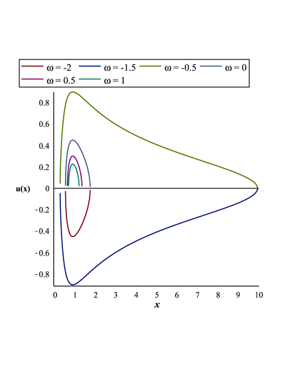
Figure 1: Velocity profile against $x=\frac{r}{M}$ for $\beta=1$, $q=1.055M$, $M=1$ and $A_{4}=0.45$ of charged RBH using Fermi-Dirac distribution.

$$\rho(r)=\frac{A_{2}(\omega+1)}{r^{3/2}\sqrt{\left(2M\left(\frac{1}{2}e^{\frac{q^{2}}{Mr}}+\frac{1}{2}\right)^{-\beta}-r\right)\left(\omega+1\right)^{2}+A^{2}_{4}r}}.$$ (29)

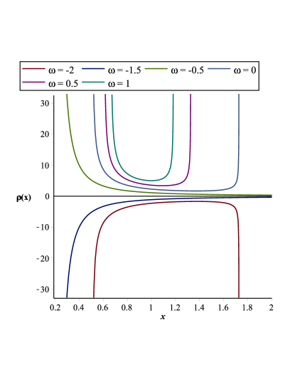
Figure 2: Energy density against $x=\frac{r}{M}$ for $\beta=1$, $q=1.055M$, $M=1$, $A_{2}=1$ and $A_{4}=0.45$ of charged RBH using Fermi-Dirac distribution.

The velocity profile for different values of $\omega$ is shown in Figure 1. Here $\omega=1,~{}0,~{}-1$ refer to stiff, dust and cosmological constant respectively and $-1<\omega<-1/3$ and $\omega<-1$ refer to quintessence and phantom energy. It can be seen that for $\omega=-1.5,~{}-2$ the radial velocity of the fluid is negative and it is positive for $\omega=-0.5,~{}0,~{}0.5,~{}1$. If the flow is outward then $u<0$ is not allowed and vice versa. In the case of $\omega=-1.5,~{}-0.5$ the fluid is at rest at $x=10$. Figure 2 represents the behavior of energy density of fluids in the surrounding area of BH. Obviously the WEC and DEC satisfied by dust, stiff and quintessence fluids. When phantom fluid ($\omega=-1.5,~{}-2$) moves towards BH then energy density decreases and reverse will happen for dust, stiff and quintessence fluids ($\omega=-0.5,~{}0,~{}0.5,~{}1$). Asymptotically $\rho~{}\rightarrow~{}0$ at infinity for $\omega=-1.5,~{}-0.5$ while it approaches to maximum at $x=1.2,~{}1.3,~{}1.8$ and near the BH.

Using this metric, Eqs.(19) and (29), the rate of change of mass of RBH due to accretion becomes

$$\dot{M}=\frac{4\pi A^{2}_{2}A_{4}(\omega+1)}{r^{3/2}\sqrt{\left(2M\left(\frac{1}{2}e^{\frac{q^{2}}{Mr}}+\frac{1}{2}\right)^{-\beta}-r\right)\left(\omega+1\right)^{2}+A^{2}_{4}r}}.$$ (30)

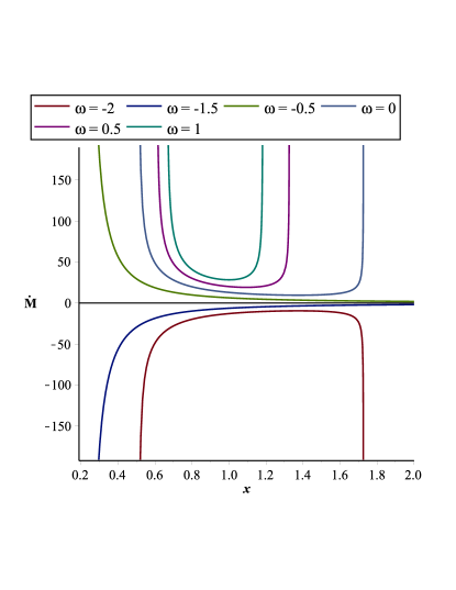
Figure 3: Rate of change of mass of RBH against $x=\frac{r}{M}$ for $\beta=1$, $q=1.055M$, $M=1$, $A_{2}=1$ and $A_{4}=0.45$ of charged RBH using Fermi-Dirac distribution.

Figure 3 represents the change in BH mass for different values of $\omega$. The mass of the BH will increase near it and at $x=1.2,~{}1.3,~{}1.7$ for $\omega=1,~{}0.5,~{}0$ respectively. On the other hand, mass of BH decrease near it and at $x=1.7$ for $\omega=-2$. Hence the mass of BH increases due to accretion of quintessence, dust and stiff matter while it decreases due to accretion phantom like fluids.

$\omega$	$r_{c}$	$u(r_{c})$	$c^{2}_{s}$
-2	1.37495	0.3138832070	.0000002580
-1.5	7.5044	0.2382908936	-.4999997476
-0.5	7.5044	-0.2382908936	-.4999997476
0	1.3749	-0.3138832070	.0000002580
0.5	1.092	-0.2476468259	0.503110174
1	0.999	-.1998921298	1.002986469

Table 1: Charged RBH using Fermi-Dirac distribution.

The critical values, critical velocities and speed of sound are obtained for different values of the EoS parameter in Table 1. Critical radius is shifting to left when $\omega\geq 0$ increases. Thus, the infalling the fluid acquires supersonic speeds closer to BH. Same critical radius is obtained for $\omega=-2,~{}0$ and $\omega=-1.5,~{}-0.5$ with same critical velocities but opposite direction. We get negative speed of sound at $x=7.5044$ and positive speed of sound for remaining critical radius. Also, the speed of sound increases near the RBH. For this metric, we find that

$$u^{2}_{c}=\frac{2^{\beta-1}\left(\left(Mr-q^{2}\right)e^{\frac{q^{2}}{\beta Mr}}+Mr\right)}{r^{2}\left(e^{\frac{q^{2}}{\beta Mr}}+1\right)^{\beta+1}},$$ (31)

$$V^{2}_{c}=\frac{2^{\beta}\left(\left(Mr-q^{2}\right)e^{\frac{q^{2}}{\beta Mr}}+Mr\right)}{2r^{2}\left(e^{\frac{q^{2}}{\beta Mr}}+1\right)^{\beta+1}-2^{\beta}\left(\left(3Mr+q^{2}\right)e^{\frac{q^{2}}{\beta Mr}}+3Mr\right)}.$$ (32)

Also, the condition (18) yields

$$\frac{2^{\beta}\left(\left(Mr-q^{2}\right)e^{\frac{q^{2}}{\beta Mr}}+Mr\right)}{r^{4}\left(e^{\frac{q^{2}}{\beta Mr}}+1\right)^{\beta+1}}>0.$$ (33)

3.2 Charged RBH Using Logistic Distribution

The Logistic distribution function is [32]

$$\xi(x)=\frac{e^{-x}}{(e^{-x}+1)^{2}},$$ (34)

in which replace $x=\frac{2q^{2}}{M\beta r}$ then we obtain the distribution function

$$\xi(\beta r)=\frac{e^{\frac{-2q^{2}}{M\beta r}}}{\left(e^{\frac{-2q^{2}}{M\beta r}}+1\right)^{2}},$$ (35)

with normalization factor is $\sigma_{\infty}=\frac{1}{4}$. Also the distribution function satisfies

$$\frac{\xi(r)}{\xi_{\infty}}\rightarrow 1,$$ (36)

where $r\rightarrow\infty$. The horizons can be obtained for $\beta=1$ where $q=1.055M$. The metric function can be written as

$$X(r)=Y(r)=1-\frac{2M}{r}\left(\frac{4e^{-\sqrt{\frac{2q^{2}}{\beta Mr}}}}{\left(e^{-\sqrt{\frac{2q^{2}}{\beta Mr}}}+1\right)^{2}}\right)^{\beta},Z(r)=r^{2}.$$ (37)

If we set $\beta\rightarrow 0$ then we obtain the Schwarzschild BH and if we set $\beta\rightarrow\infty$ we get

$$X(r)=Y(r)=1-\frac{2M}{r}e^{\frac{-q^{2}}{2Mr}}.$$ (38)

It is noteworthy that this metric function corresponds to an Ay on-Beato and Garc a BH [32].

The radial velocity and energy density for the metric (37) using eqs. (5) and (10) is given by

$$u(r)=\frac{1}{(\omega+1)\sqrt{r}}\left(\left(-2M\left(\frac{4e^{-\sqrt{\frac{2q^{2}}{\beta Mr}}}}{\left(e^{-\sqrt{\frac{2q^{2}}{\beta Mr}}}+1\right)^{2}}\right)^{\beta}+r\right)\left(\omega+1\right)^{2}-A^{2}_{4}r\right)^{1/2},$$ (39)

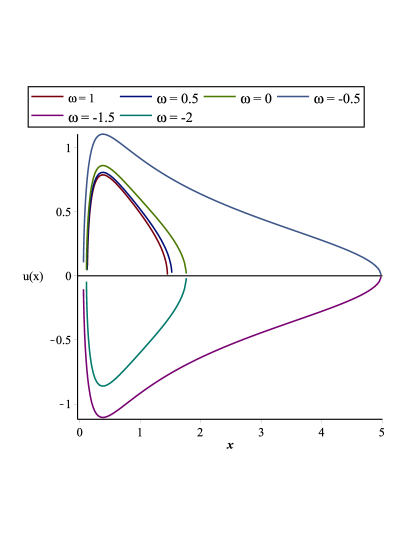
Figure 4: Velocity profile against $x=\frac{r}{M}$ for $\beta=1$, $q=1.055M$, $M=1$ and $A_{4}=0.4$ of charged RBH using logistic distribution.

$$\rho(r)=-\frac{A_{2}(\omega+1)}{r^{3/2}\left(\left(2M\left(\frac{4e^{-\sqrt{\frac{2q^{2}}{\beta Mr}}}}{\left(e^{-\sqrt{\frac{2q^{2}}{\beta Mr}}}+1\right)^{2}}\right)^{\beta}-r\right)\left(\omega+1\right)^{2}+A^{2}_{4}r\right)^{1/2}}.$$ (40)

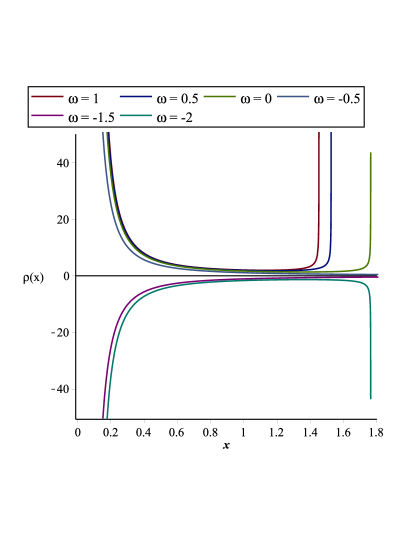
Figure 5: Energy density against $x=\frac{r}{M}$ for $\beta=1$, $q=1.055M$, $M=1$, $A_{2}=1$ and $A_{4}=0.4$ of charged RBH using logistic distribution.

The velocity profile for different values of $\omega$ is shown in Figure 4. It can be observed that for $\omega=-1.5,~{}-2$ the radial velocity of the fluid is negative and it is positive for $\omega=-0.5,~{}0,~{}1$. If the flow is inward then $u>0$ is not allowed and vice versa. In the case of $\omega=-2,~{}0$ the fluid is at rest at $x~{}\approx~{}5$. Figure 5, represents the behavior of energy density of fluids in the surrounding area of BH. Obviously the WEC and DEC are satisfied by dust, stiff and quintessence fluids. When phantom like fluid ($\omega=-1.5,~{}-2$) moves towards BH then energy density decreases and reverse will happen for dust, stiff and quintessence fluids ($\omega=-0.5,~{}0,~{}0.5,~{}1$).

The $\dot{M}$ of RBH for distinct EoS parameters is obtained by using (19)

$$\dot{M}=-\frac{4\pi A^{2}_{2}A_{4}(\omega+1)}{r^{3/2}\left(\left(2M\left(\frac{4e^{-\sqrt{\frac{2q^{2}}{\beta Mr}}}}{\left(e^{-\sqrt{\frac{2q^{2}}{\beta Mr}}}+1\right)^{2}}\right)^{\beta}-r\right)\left(\omega+1\right)^{2}+A^{2}_{4}r\right)^{1/2}}.$$ (41)

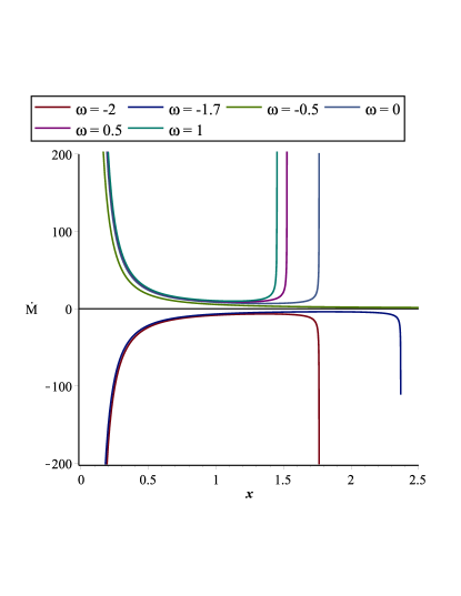
Figure 6: Rate of change of mass of RBH against $x=\frac{r}{M}$ for $\beta=1$, $q=1.055M$, $M=1$, $A_{2}=1$ and $A_{4}=0.4$ of charged RBH using logistic distribution.

Figure 6 represents the change in BH mass against x. It is evident that the mass of BH increases due to quintessence, dust and stiff fluids and it decreases due to phantom fluids.

$\omega$	$r_{c}$	$u(r_{c})$	$c^{2}_{s}$
-2	1.36375	-0.3998729763	-0.1018620364
-1.5	3.777412	-0.3138895411	-0.5007414180
-0.5	3.77412	0.3138895411	-0.5007414180
0	1.36375	0.3998724197	-0.1018620364
0.5	1.1850	0.4018068205	0.116622918
1	1.12974	0.4014558621	0.231766770

Table 2: Charged RBH using logistics distribution.

The critical radius, critical velocities and speed of sound are obtained for different values of EoS parameter in Table 2. Critical radius is shifting to right when $\omega\geq 0$ increases. Thus the infalling the fluid acquires supersonic speeds closer to BH. For phantom like fluid, quintessence, dust and stiff matter the critical radius and critical velocities are explained in the above table. Same critical radius is obtained for $\omega=-2,~{}0$ and $\omega=-1.5,~{}-0.5$ with same critical velocities but differ in sign. We obtained negative speed of sound at $x=1.36375,~{}3.777412$ and positive speed of sound at $x=1.12974,~{}1.1850$. Near the BH speed of sound will increase. For this metric we find that

$$u^{2}_{c}=\frac{2^{-2+2\beta}\sqrt{M}e^{\sqrt{\frac{2q^{2}\beta}{Mr}}}\left(\left(\sqrt{2}q\beta+2\sqrt{\beta Mr}\right)+\left(-\sqrt{2}q\beta+2\sqrt{\beta Mr}\right)e^{\sqrt{\frac{2q^{2}\beta}{Mr}}}\right)}{\sqrt{\beta}r^{3/2}\left(e^{\sqrt{\frac{2q^{2}\beta}{Mr}}}\right)},$$ (42)

$$V^{2}_{c} = \left(2^{\beta}Me^{\sqrt{\frac{2q^{2}\beta}{Mr}}}\left(\left(\sqrt{2}q\beta+2\sqrt{\beta Mr}\right)+\left(-\sqrt{2}q\beta+2\sqrt{\beta Mr}\right)e^{\sqrt{\frac{2q^{2}\beta}{Mr}}}\right)\right)$$ (43)

$$\left(4\sqrt{\beta M}r^{3/2}\left(e^{\sqrt{\frac{2q^{2}\beta}{Mr}}}\right)-2^{\beta}e^{-\sqrt{\frac{2\beta q^{2}}{Mr}}}\left(\left(-\sqrt{2}Mq\beta+6\sqrt{\beta r}M^{3/2}\right)\right.\right.$$

$$\left.\left.e^{-\sqrt{\frac{2q^{2}}{\beta Mr}}}+\sqrt{2}Mq\beta+6\sqrt{\beta r}M^{3/2}\right)\right)^{-1}.$$

Also, the condition (18) yields

$$\frac{2^{-1+2\beta}\sqrt{M}e^{-\sqrt{\frac{2q^{2}\beta}{Mr}}}\left(\left(\sqrt{2}q\beta+2\sqrt{\beta Mr}\right)e^{-\sqrt{\frac{2q^{2}\beta}{Mr}}}+\left(-\sqrt{2}q\beta+2\sqrt{\beta Mr}\right)\right)}{\sqrt{\beta}r^{7/2}\left(e^{\sqrt{\frac{2q^{2}\beta}{Mr}}}\right)}>0$$ (44)

3.3 Charged RBH from Nonlinear Electrodynamics

Using the line element

$$X(r)=Y(r)=1-\frac{2M(r)}{r}.$$ (45)

Here the function

$$M(r)=M\left(1-tanh\left(\frac{q^{2}}{2Mr}\right)\right),$$ (46)

and its associated electric field source is

$$E=\frac{q}{r^{2}}\left(1-tanh^{2}\left(\frac{q^{2}}{2Mr}\right)\right)\left(1-\frac{q^{2}}{4Mr}tanh\left(\frac{q^{2}}{2Mr}\right)\right),$$ (47)

where q and M represent electric charge and mass respectively [33]. The solution elaborate RBH and its global structure is like R-N BH. The asymptotic behavior of the solution is

$$X(r)=1-\frac{2M}{r}+\frac{q^{2}}{r^{2}}+O\left(\frac{1}{r^{4}}\right).$$ (48)

So the metric function

$$X(r)=Y(r)=1-\frac{2M}{r}\left(M\left(1-tanh(\frac{q^{2}}{2Mr})\right)\right),Z(r)=r^{2}.$$ (49)

The radial velocity and energy density for this metric are given by

$$u(r)=\frac{\sqrt{\left(-2Mtanh\left(\frac{q^{2}}{2Mr}\right)+2M-r\right)\left(\omega+1\right)^{2}+A^{2}_{4}r}}{(\omega+1)\sqrt{r}},$$ (50)

$$\rho(r)=\frac{(\omega+1)A_{2}}{r^{3/2}\sqrt{\left(-2Mtanh(\frac{q^{2}}{2Mr}+2M-r)\right)\left(\omega+1\right)^{2}+A^{2}_{4}r}}.$$ (51)

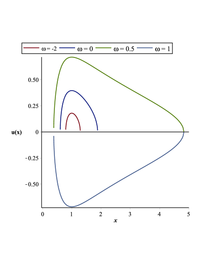
Figure 7: Velocity profile against $x=\frac{r}{M}$ for $q=1.055M$, $M=1$ and $A_{4}=0.7$ of charged RBH from nonlinear electrodynamics.

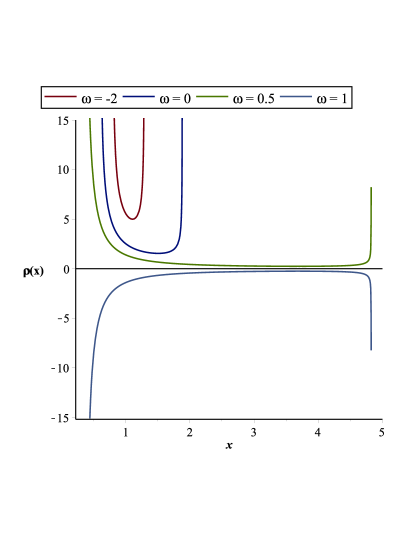
Figure 8: Energy density against $x=\frac{r}{M}$ for $q=1.055M$, $M=1$, $A_{2}=1$ and $A_{4}=0.7$ of charged RBH from nonlinear electrodynamics.

The absolute value of the velocity profile for different values of $\omega$ is shown in Figure 7. It can be observed that for $\omega=-2$ the radial velocity of the fluid is negative and it is positive for $\omega=0.5,~{}0,~{}1$. If the flow is inward then $u>0$ is not allowed and vice versa. In the case of $\omega=-2,~{}0$ the fluid is at rest at $x\approx 5$. Figure 8 represents the energy density of fluids in the region of BH. It is apparent that the WEC and DEC is satisfied by phantom fluids. When phantom fluids moves towards the BH the energy density increases on the other hand it decreases for dust and stiff matter.

The rate of change of mass is given by

$$\dot{M}=-\frac{4\pi A^{2}_{2}A_{4}(\omega+1)}{r^{3/2}\sqrt{\left(-2Mtanh(\frac{q^{2}}{2Mr}+2M-r)\right)\left(\omega+1\right)^{2}+A^{2}_{4}r}}.$$ (52)

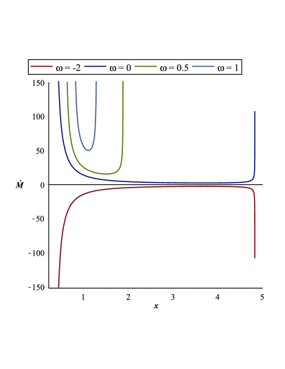
Figure 9: Rate of change of mass of RBH against $x=\frac{r}{M}$ for $q=1.055M$, $M=1$, $A_{2}=1$ and $A_{4}=0.7$ of charged RBH from nonlinear electrodynamics.

The rate of change of in the BH mass against x is plotted in Figure 9. Due to accretion of dust and stiff matter the mass of the BH will increase for small values of x and vice versa for phantom fluids. It is also noted that the maximum rate of RBH mass increases due to $\omega~{}=~{}1$ followed by $\omega=0.5,~{}0,~{}-2$.

$\omega$	$r_{c}$	$u(r_{c})$	$c^{2}_{s}$
-2	3.685523529	-0.2993097288	-0.125
0	3.685523529	0.2993097288	-0.125
0.5	1.506050868	0.2844719573	0.312500584
1	1.106971797	0.1633564212	0.750003072

Table 3: Charged RBH from nonlinear electrodynamics.

The critical values, critical velocities and speed of sound are obtained for different values of EoS parameter in Table 3. Critical radius is shifting to right when $\omega\geq 0$ increases. Speed of sound is negative at $x=3.685523529$ and near the BH the speed of sound will increase. For this RBH we find that

$$u^{2}_{c}=\frac{q^{2}\left(tanh^{2}\left(\frac{q^{2}}{2Mr}\right)-1\right)+2Mr\left(-tanh\left(\frac{q^{2}}{2Mr}\right)+1\right)}{4r^{2}},$$ (53)

$$V^{2}_{c}=\frac{q^{2}\left(tanh^{2}\left(\frac{q^{2}}{2Mr}\right)-1\right)+2Mr\left(-tanh\left(\frac{q^{2}}{2Mr}\right)+1\right)}{4r^{2}+q^{2}\left(tanh^{2}\left(\frac{q^{2}}{2Mr}\right)-1\right)+6+Mr\left(tanh\left(\frac{q^{2}}{2Mr}\right)-1\right)}.$$ (54)

Also, the condition (18) yields

$$\frac{\left(tanh^{2}\left(\frac{q^{2}}{2Mr}\right)-1\right)q^{2}+2Mr\left(-tanh\left(\frac{q^{2}}{2Mr}\right)+1\right)}{2r^{4}}>0.$$ (55)

3.4 Kehagias - Sftesos asymptotically flat BH

KS studied the following BH metric

$$X(r)=Y(r)=1+br^{2}-\sqrt{b^{2}r^{4}+4Mbr},Z(r)=r^{2}.$$ (56)

In the frame work of Horava theory, where m is the mass, b is the positive constant related to coupling constant of theory. The metric asymptotically behaves the usual Schwarzschild BH [34]

$$X(r)=Y(r)\approx 1-\frac{2M}{r}+O\left(\frac{1}{r^{4}}\right),$$ (57)

for $r\gg(\frac{r}{b})^{1/3}$. The KS metric have two horizons at

$$r_{\pm}=M\left(1\pm\sqrt{\left(1-\frac{1}{2bM^{2}}\right)}\right),$$ (58)

with $2bM^{2}\geq 1$ [34].

The radial velocity and energy density are given by

$$u(r)=\frac{\left(A^{2}_{4}+\left(\sqrt{b^{2}r^{4}+4Mbr}-br^{2}-1\right)\left(\omega+1\right)^{2}\right)^{1/2}}{\omega+1},$$ (59)

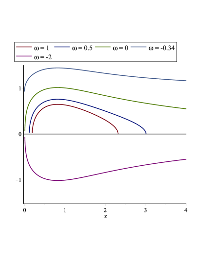
Figure 10: Velocity profile against $x=\frac{r}{M}$ for $M=1$, $b=0.9$ and $A_{4}=0.9$ of Kehagias - Sftesos asymptotically flat BH.

$$\rho(r)=\frac{A_{2}(\omega+1)}{r^{2}\left(A^{2}_{4}+\left(\sqrt{b^{2}r^{4}+4Mbr}-br^{2}-1\right)\left(\omega+1\right)^{2}\right)^{1/2}}.$$ (60)

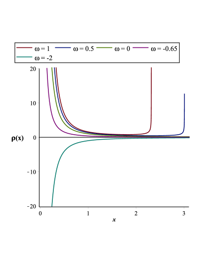
Figure 11: Energy density against $x=\frac{r}{M}$ for $M=1$, $A_{2}=1$, $b=0.9$ and $A_{4}=0.9$ of Kehagias - Sftesos asymptotically flat BH.

The radial velocity for different values of $\omega$ is shown in Figure 10. The radial velocity is negative for phantom like fluid and positive for quintessence, dust and stiff matter. The evolution of energy density of fluids in the surrounding area of RBH is plotted in Figure 11. The energy density for phantom fluids is negative while the energy density for stiff, dust and quintessence fluids is positive.

For this RBH, rate of change of mass becomes

$$\dot{M}=\frac{4\pi A^{2}_{2}A_{4}(\omega+1)}{r^{2}\left(A^{2}_{4}+\left(\sqrt{b^{2}r^{4}+4Mbr}-br^{2}-1\right)\left(\omega+1\right)^{2}\right)^{1/2}}.$$ (61)

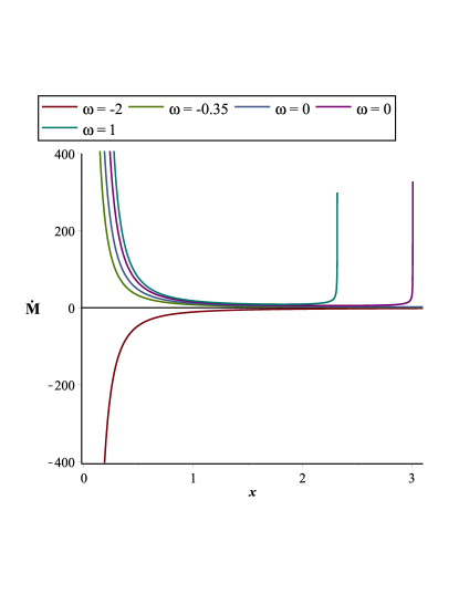
Figure 12: Rate of change of mass of RBH against $x=\frac{r}{M}$ for $M=1$, $A_{2}=1$, $b=0.9$ and $A_{4}=0.9$ of Kehagias - Sftesos asymptotically flat BH.

Figure 11 represents the rate of change in RBH mass against x. We see that the RBH mass will increase for $\omega=-0.35,~{}0,~{}0.5,~{}1$ and it will decrease for $\omega=-2$.

$\omega$	$r_{c}$	$u(r_{c})$	$c^{2}_{s}$
-2	7.8946	-0.2505321935	0.0000008330
-0.34	30267.74	0.6327458490	-0.0513167023
0	7.8946	0.2505321736	0.0000008330
0.5	2.3185	0.3961993774	0.500013404
1	1.8183	0.3888079314	0.500013404

Table 4: Kehagias - Sftesos asymptotically flat BH.

The critical values, critical velocities and speed of sound for different values of $\omega$ is presented in the Table 4. For quintessence matter, we obtain very large critical radius. Similarly as before, we obtain the same critical radius for dust and phantom like fluids and same critical velocities but differ in sign. If we increase the EoS parameter then the critical radius is shifted near RBH. It is evident that the critical velocity is negative for phantom like fluid and positive for quintessence, dust and stiff matter. The speed of sound is negative at $x=30267.74$ and positive for remaining critical radius. For this metric, we find that

$$u^{2}_{c}=\frac{r}{4}\left(2br-\frac{2b^{2}r^{3}+2Mb}{\sqrt{r\left(b^{2}r^{3}+4Mb\right)}}\right),$$ (62)

$$V^{2}_{c}=\frac{r^{2}\left(2br-\frac{2b^{2}r^{3}+2Mb}{\sqrt{r\left(b^{2}r^{3}+4Mb\right)}}\right)}{r^{2}\left(2br-\frac{2b^{2}r^{3}+2Mb}{\sqrt{r\left(b^{2}r^{3}+4Mb\right)}}\right)+4r\left(1+br^{2}-{\sqrt{r\left(b^{2}r^{3}+4Mb\right)}}\right)}.$$ (63)

The condition (18) becomes

$$\frac{\left(2br-\frac{2b^{2}r^{3}+2Mb}{\sqrt{r\left(b^{2}r^{3}+4Mb\right)}}\right)}{2r}>0.$$ (64)

4 Concluding Remarks

In this work, we have investigated the accretion onto various RBHs (such as RBH using Fermi-Dirac Distribution, RBH using logistic distribution, RBH using nonlinear electrodynamics and Kehagias-Sftesos asymptotically flat RBH) which are asymptotically leads to Schwarzschild and Reissner-Nordstrom BHs (most of them satisfy the WEC). We have followed the procedure of Bahamonde and Jamil [22] and obtained the critical points, critical velocities and the behavior of sound speed for chosen RBHs. Moreover, we have analyzed the behavior of radial velocity, energy density and rate of change of mass for RBHs for various EoS parameters. For calculating these quantities, we have assumed the barotropic EoS and found the relationship between the conservation law and barotropic EoS. We have found that the radial velocity ($u$) of the fluid is positive for stiff, dust and quintessence matter and it is negative for phantom-like fluids. If the flow is inward then $u<0$ is not allowed and $u>0$ is not allowed for outward flow. Also, we have obtained that the energy density remains positive for quintessence, dust and stiff matter while becomes negative for phantom-like fluid near RBHs.

In addition, the rate of mass of BH is dynamical quantity, so the analysis of the nature its mass in the presence of various dark energy models may become very interesting in the present scenario. Also, the sensitivity (increasing or decreasing) of BHs mass depend upon the nature of fluids which accretes onto it. Therefore, we have considered the various possibilities of accreting fluids such as dust and stiff matter, quintessence and phantom. We have found that the rate of change of mass of all RBHs increases for dust and stiff matter, quintessence-like fluid since these fluids do not have enough repulsive force. However, the mass of all RBHs decreases in the presence of phantom-like fluid (and the corresponding energy density and radial velocity becomes negative) because it has strong negative pressure. This result shows the consistency with several works [22, 31, 35, 36, 37, 38, 39]. Also, this result favor the phenomenon that universe undergoes the big rip singularity, where all the gravitationally bounded objects dispersed due to phantom dark energy.

Although, we have assumed the static fluid which may be extended for non-static fluid without assuming any EoS and can be obtained more interesting results. This is left for future considerations.

References

- [1] Perlmutter, et al., S.: Supernova Cosmology Project Collaboration. Astrophys. J. 517, 565 (1999).
- [2] Spergel, et al., D.N.: WMAP Collaboration. Astrophys. J. Suppl. 170, 377 (2007).
- [3] Eisenstein, et al., D.J.: SDSS Collaboration. Astrophys. J. 633, 560 (2005).
- [4] Riess, et al., A.G.: Supernova Search Team Collaboration. Astron. J. 116, 1009 (1998).
- [5] Johri, V.B.: Phys. Rev. D 70, 041303 (2004).
- [6] Lobo, F.S.N.: Phys. Rev. D 71, 084011 (2005).
- [7] Nojiri, S. and Odintsov, S.: Phys. Rep. 505, 59 144 (2011).
- [8] Armendariz-Picon, C., Mukhanov, V.F. and Steinhardt, P.J.: Phys. Rev. Lett. 85, 4438 (2000).
- [9] Gasperini, et al., M.: Phys. Rev. D 65, 023508 (2002).
- [10] Gumjudpai, B. and Ward, J.: Phys. Rev. D 80, 023528 (2009).
- [11] Martin, J. and Yamaguchi, M.: Phys. Rev. D 77, 123508 (2008).
- [12] Wei, H., Cai, R.G. and Zeng, D.F.: Class. Quant. Grav. 22, 3189 (2005).
- [13] Sen, A.: JHEP 0207, 065 (2002).
- [14] Caldwell, R.R.: Phys. Lett. B 545, 23 (2002).
- [15] Kamenshchik, A.Y., Moschella, U. and Pasquier, V.: Phys. Lett. B 511, 265 (2001).
- [16] Copeland, E.J., Sami, M. and Tsujikawa,S.: Int. J. Mod. Phys. D 15, 1753 (2006).
- [17] Elizalde, E. and Hildebrandt, S. R.: Phys. Rev. D 65, 124024 (2002).
- [18] Zaslavskii, O. B.: Phys. Lett. B 688, 278 (2010).
- [19] Hawking, S.W. and Ellis, G.F.: The Large Scale Structure of Space Time (Cambridge Univ. Press 1973).
- [20] Senovilla, J.M.M.: Gen. Relat. Gravt. 30, 701 (1998).
- [21] Bardeen, J.: presented at GR5, Tiflis, U.S.S.R., and published in the conference proceedings in the U.S.S.R. (1968).
- [22] Bahamonde, S. and Jamil, M.: Eur. Phys. J. C 75, 508 (2015).
- [23] Bondi, H.: Mon. Not. R. Astron. Soc. 112, 195 (1952).
- [24] Michel, F.C.: Astrophys. Space Sci. 15, 153 (1972).
- [25] Babichev, et al., E.: Phys. Rev. Lett. 93, 021102 (2004).
- [26] Babichev, E., Dokuchaev, V. and Eroshenko, Y.: J. Exp. Theor. Phys. 100, 528 538 (2005).
- [27] Jamil, M.: Eur. Phys. J. C 62, 609 (2009).
- [28] Sharif, M. and Abbas, G.: Chin. Phys. Lett. 29, 010401 (2012).
- [29] Kim, S.W. and Kang, Y.: Int. J. Mod. Phys. Conf. Ser. 12, 320 (2012).
- [30] Jimenez, Madrid, J.A. and Gonzalez-Diaz, P.F.: Grav. Cosmol. 14, 213 (2008).
- [31] Debnath, U.: Eur. Phys. J. C 75, 129 (2015).
- [32] Leonardo, Balart and Elias, C. Vagenas: Phys. Rev. D 90, 124045 (2014).
- [33] Sharif, M. and Jawad, A.: Mod. Phys. Lett. A 25, 3241-3250(2010).
- [34] Culetu, H.: Astrophys. Space Sci. 2, 360(2015).
- [35] Debnath, U.: Eur. Phys. J. C 75, 449 (2015).
- [36] Wei, H.: Class. Quantum Grav. 29(2012)175008.
- [37] Lobo, F.S.N.: Phys. Rev. D 71(2005)124022; Lobo, F.S.N.: Phys. Rev. D 71(2005)084011; Sushkov, S.: Phys. Rev. D 71(2005)043520.
- [38] Babichev, E., Dokuchaev, V. and Eroshenko, Y.: Phys. Rev. Lett. 93(2004)021102.
- [39] Sharif, M. and Abbas, G.: Chin. Phys. Lett. 28(2011)090402; Martin-Moruno, P.: Phys. Lett. B 659(2008)40; Jamil, M., Rashid, M.A. and Qadir, A.: Eur. Phys. J. C 58(2008)325; Babichev, E. et al.: Phys. Rev. D 78(2008)104027; Jamil, M.: Eur. Phys. J. C 62(2009)325; Jamil, M. and Qadir, A.: Gen. Rel. Grav. 43(2011)1069; Bhadra, J. and Debnath, U.: Eur. Phys. J. C 72(2012)1912.