First-forbidden $\mathbf{\beta}$-decay rates, energy rates of $\beta$-delayed neutrons and probability of $\beta$-delayed neutron emissions for neutron-rich nickel isotopes.

Abstract

First-forbidden (FF) transitions can play an important role in decreasing the calculated half-lives specially in environments where allowed Gamow-Teller (GT) transitions are unfavored. Of special mention is the case of neutron-rich nuclei where, due to phase-space amplification, FF transitions are much favored. We calculate the allowed GT transitions in various pn-QRPA models for even-even neutron-rich isotopes of nickel. Here we also study the effect of deformation on the calculated GT strengths. The FF transitions for even-even neutron-rich isotopes of nickel are calculated assuming the nuclei to be spherical. Later we take into account deformation of nuclei and calculate GT + unique FF transitions, stellar $\beta$-decay rates, energy rate of $\beta$-delayed neutrons and probability of $\beta$-delayed neutron emissions. The calculated half-lives are in excellent agreement with measured ones and might contribute in speeding-up of the $r$-matter flow.

1 Introduction

Exotic nuclei exhibiting high isospin values and located far from stability line have gained amplified interest. The reason for this is twofold. Unprecedented features are predicted with recent theoretical development when moving towards the neutron drip line and away from the valley of stability Dob94 . Changing of the traditional shell gaps and magic numbers, spin-orbit interaction weakening and dilute neutron matter are some of the examples of these features. The study of nuclei structure and its understanding when put under extreme conditions can shed new light on the effective nucleon-nucleon interaction choice in the nuclear medium. Following to this, the so called neutron-rich exotic nuclei are believed to play a crucial role in explosive nucleosynthesis phenomenon like the different $r$-processes in supernovae events Kra93 .

It is commonly accepted that $r$-process occurs in an explosive environment of relatively high temperatures (T $\thickapprox$ 10⁹ K) and very high neutron densities ($>$10²⁰ cm^-3) Kra93 ; Bur57 ; Cam57 ; Cow91 ; Woo94 . Neutron captures, under such conditions, are observed much faster than competing $\beta$-decays and the $r$-process path in the nuclear chart proceeds through a chain of extremely neutron-rich nuclei with approximately constant and relatively low neutron separation energies (S_n $\lesssim$ 3 MeV). They form a chain through which the $r$-process path appears to proceed in the nuclear chart. The neutron separation energies show discontinuities at the magic numbers N = 50, 82, and 126 due to the relatively stronger binding of nuclei with magic neutron numbers. The $r$-matter flow, in consequence, slows down when it approaches these magic neutron nuclei and here it waits for several $\beta$-decays (which are also longer than for other nuclei on the $r$-process path) to occur before further neutron captures are possible, carrying the mass flow to heavier nuclei. Thus matter is accumulated at these $r$-process waiting points associated with the neutron numbers N = 50, 82, and 126, leading to the well-known peaks in the observed $r$-process abundance distribution.

Practically in all stellar processes, e.g., massive stars hydrostatic burning, pre-supernova evolution of massive stars and nucleosynthesis ($s$-, $p$-, $r$-, $rp$-) processes, the weak interaction rates are the important ingredients and play a crucial role Bur57 . Stellar weak interaction processes, for densities $\rho\lesssim$ 10¹¹ g/cm³, are dominated by Gamow-Teller (GT) and also by Fermi transitions if applicable. The contribution of forbidden transitions is observed sizeable for nuclei lying in the vicinity of $\beta$ stability line for density $\rho\geq$ 10¹¹ g/cm³ and electron chemical potential of the order of 30 MeV or more Coo84 . However recent studies have shown the importance of forbidden transitions also at orders of magnitude lower densities Nab13 ; Zhi13 . The QRPA studies based on the Fayans energy functional has been extended by Borzov recently for a consistent treatment of allowed and first-forbidden (FF) contributions to $r$-process half-lives Bor06 . A significant reduction in the half-lives of N = 126 is seen while these calculations find that forbidden contributions give only a small correction to the half-lives of the N = 50 and N = 82. The correlations among nucleons are expected to not only affect the half-lives, but to give a reliable description of the detailed allowed and forbidden strength functions. This description is indeed needed to estimate the energy rate of neutron from daughter nuclei and probabilities for beta-delayed neutron emission rates which are known to be important to describe the decay of the $r$-process nuclei towards stability after freeze-out.

The $\beta$-decay properties, under terrestrial conditions, of allowed weak interaction and U1F Hom96 led to a better understanding of the $r$-process. Authors in Hom96 showed that for near-stable and near-magic nuclei a large contribution to the total transition probability came from U1F transitions. To describe the isotopic dependence of the $\beta$-decay characteristics the allowed $\beta$-decay approximation alone is not sufficient Bor06 , specially for the nuclei crossing the closed N and Z shells for which forbidden transitions give a dominant contribution to the total half-life (specially for N $>$ 50 in ⁷⁸Ni region). A large-scale shell-model calculation of the half-lives, including first-forbidden contributions, was also performed for $r$-process waiting-point nuclei Zhi13 . Since the weak interaction rates are of decisive importance in the domains of high temperature and density therefore there was a need to perform these calculations under stellar conditions. The microscopic calculations of allowed GT and unique first-forbidden (U1F) rates for nickel isotopes in stellar environment were performed recently using the pn-QRPA model Nab13 . This study suggested to also incorporate rank 0 and rank 1 operators for a full coverage of FF transitions and much better comparison with measured half-lives.

The pn-QRPA model was developed by Halbleib and Sorensen Hal67 by generalizing the usual RPA to describe charge-changing transitions. A microscopic approach based on the proton neutron quasi-particle random phase approximation (pn-QRPA), have so far been successfully used in studies of nuclear $\beta$-decay properties of stellar weak-interaction mediated rates (see Nab99 ; Nab99a ; Nab04 ). The pn-QRPA model allows a state-by-state evaluation of the weak rates by summing over Boltzmann-weighted, microscopically determined GT strengths for all parent excited states. Construction of a quasi-particle basis is first performed in this model with a pairing interaction, and then the RPA equation is solved with GT residual interaction.

This paper can be broadly categorized into two different calculations. Both calculations employ pn-QRPA methods using two different potentials. The first calculation deals with the allowed GT strength of even-even spherical and deformed isotopes of neutron-rich nickel isotopes using the Woods-Saxon potential. Here we use three different versions of the pn-QRPA model and tag them as pn-QRPA(WS-SSM), pn-QRPA(WS-SPM) and pn-QRPA(WS-DSM) models for spherical and deformed cases, respectively. The FF contributions were calculated using only the pn-QRPA(SSM) model. The second pn-QRPA calculation employs a deformed Nilsson potential and is referred to as pn-QRPA(N) model. All models would be introduced in the next section. The pn-QRPA(N) model was used to calculate GT+U1F transitions, $\beta$-decay and positron capture rates, energy rate of emitted neutrons from daughter nuclei and probability of $\beta$-delayed neutron emissions. All pn-QRPA(N) calculations were further performed in stellar environment.

The paper is organized in four sections. Section 2 briefly describes the formalism of the various pn-QRPA models used in this paper. In Section 3, we discuss the results of allowed GT and FF strength distributions, phase space calculations, half-lives, stellar $\beta$-decay and positron capture rates, energy rate of neutrons and probability of $\beta$-delayed neutron emissions for the neutron-rich nickel isotopes. Section 4 finally concludes our findings.

2 Formalism

As discussed earlier, this paper can be broadly divided into two different set of calculations using pn-QRPA models with different single-particle potentials. In this section we briefly describe the formalism to perform the respective calculations using the different models.

2.1 The pn-QRPA(WS) model

Allowed beta decay half-lives have been calculated using deformed schematic model (DSM), spherical schematic model (SSM) and spherical Pyatov’s method (SPM) within the framework of pn-QRPA(WS) method. The Woods-Saxon potential with Chepurnov parametrization has been used as a mean field basis in numerical calculations. The eigenvalues and eigenfunctions of the Hamiltonian with separable residual GT effective interactions in particle-hole (ph) channel were solved within the framework of pn-QRPA model.

We constructed a quasi-particle basis described by a Bogoliubov transformation and solved the RPA equation with a schematic residual GT interaction

$$a_{j_{p}m_{p}}=U_{j_{p}}\alpha_{j_{p}m_{p}}+(-1)^{j_{p}-m_{p}}V_{j_{p}}\alpha^{+}_{j_{p}-m_{p}}$$

$$a^{+}_{j_{n}m_{n}}=U_{j_{n}}\alpha^{+}_{j_{n}m_{n}}+(-1)^{j_{n}-m_{n}}V_{j_{n}}\alpha_{j_{n}-m_{n},}$$

where $U_{j_{n}}(U_{j_{p}})$, $V_{j_{n}}(V_{j_{p}})$, $a^{+}_{j_{n}m_{n}}(a_{j_{p}m_{p}})$ and $\alpha^{+}_{j_{n}m_{n}}(\alpha_{j_{p}m_{p}})$ are the standard BCS occupation amplitudes, the nucleon creation (annihilation) and the quasi-particle creation (annihilation) operators, respectively. We considered a system of nucleons in a deformed mean field with pairing forces. The single quasi-particle (sqp) Hamiltonian of the system can be defined using

$$\hat{H}_{sqp}=\sum_{j_{\tau}m_{\tau}}[\varepsilon_{j_{n}}\alpha^{+}_{j_{n}m_{n}}\alpha_{j_{n}m_{p}}+\varepsilon_{j_{p}}\alpha^{+}_{j_{p}m_{p}}\alpha_{j_{p}m_{p}}],~{}~{}~{}~{}\tau=n,p$$

where $\varepsilon_{j_{\tau}}$ are the energies of neutron(proton) quasi-particle

$$\varepsilon_{j_{\tau}}=\sqrt{(E_{j_{\tau}}-\lambda)^{2}+\Delta^{2}}.$$

Here $E_{j_{\tau}}$, $\lambda$ and $\Delta$ are the single particle neutron(proton) energy, the chemical potential and pairing energies, respectively. Charge-exchange spin-spin correlations are added to the model Hamiltonian in the following form

$$\hat{V}_{\beta}=2\chi_{\beta}\sum_{\beta}\beta^{+}_{\mu}\beta^{-}_{\mu},~{}~{}~{}~{}~{}~{}\mu=0,\pm 1$$

where $\beta^{+}_{\mu}(\beta^{-}_{\mu})$ is the positron(electron) decay operator

$$\beta^{+}_{\mu}=\sum_{n\rho}\sum_{p\rho^{{}^{\prime}}}<n\rho|\sigma_{\mu}+(-1)^{\mu}\sigma_{-\mu}|p\rho^{{}^{\prime}}>a^{+}_{n\rho}a_{p\rho^{{}^{\prime}}},~{}~{}~{}~{}~{}~{}\beta^{-}_{\mu}=({\beta^{+}_{\mu}})^{{\dagger}}$$

and $\sigma_{\mu}$ is and the spherical component of the Pauli operator. The main formulae are given here. Details mathematical formalism are available in Gab70 ; Ayg02 ; Sel03 ; Sel04 .

The total pn-QRPA Hamiltonian for deformed nuclei is described as

$$\hat{H}_{DSM}=\hat{H}_{sqp}+\hat{V}_{\beta}.$$ (1)

The total Hamiltonian in Pyatov’s method is given by

$$\hat{H}_{SPM}=\hat{H}_{av}+\hat{V}_{\beta}+\hat{h}_{0},$$ (2)

where $\hat{H}_{av}$ is the single quasi-particle Hamiltonian in a spherical symmetric average field with pairing forces. The third term comes from the restoration of broken commutation relation between the nuclear Hamiltonian and the GT operator. The schematic method Hamiltonian for GT excitations in the neighbor odd-odd nuclei is given by

$$\hat{H}_{SSM}=\hat{H}_{av}+\hat{V}_{\beta}.$$ (3)

Details of solution of allowed GT formalism can be seen in Cak10a ; Cak12 .

The ft values for the allowed GT $\beta$ transitions are finally calculated using

$$ft=\frac{D}{(\frac{g_{A}}{g_{V}})^{2}4\pi B^{GT}(I_{i}\rightarrow I_{f},\beta^{-})},$$

where the reduced matrix elements of GT transitions are given by

$$B^{GT}(I_{i}\rightarrow I_{f},\beta^{-})=\sum_{\mu}|\langle 1^{+}_{i},\mu|G_{\mu}^{-}|0^{+}\rangle|^{2}.$$

The model Hamiltonian which generates the spin-isospin dependent vibration modes with $\lambda^{\pi}=0^{-},1^{-},2^{-}$ in odd-odd nuclei in quasi boson approximation is given as

$$\hat{H}=\hat{H}_{sqp}+\hat{h}_{ph}.$$ (4)

The single quasi-particle Hamiltonian of the system is given by

$$\hat{H}_{sqp}=\sum_{j_{\tau}}\varepsilon_{j_{\tau}}\alpha^{{\dagger}}_{j_{\tau}m_{\tau}}\alpha_{j_{\tau}m_{\tau}}~{}~{}(\tau=p,n),$$

where $\varepsilon_{j_{\tau}}$ and $\alpha^{+}_{j_{\tau}m_{\tau}}(\alpha_{j_{\tau}m_{\tau}})$ are the single quasi-particle energy of the nucleons with angular momentum ${j_{\tau}}$ and the quasi-particle creation (annihilation) operators, respectively.

The $\hat{h}_{ph}$ is the spin-isospin effective interaction Hamiltonian which generates $0^{-}$,$1^{-}$,$2^{-}$ vibration modes in particle-hole channel and given as

$$\hat{h}_{ph}=\frac{2\chi_{ph}}{g_{A}^{2}}\sum_{j_{p}j_{n}j_{p^{\prime}}j_{n^{\prime}}\mu}[b_{j_{p}j_{n}}A^{+}_{j_{p}j_{n}}(\lambda\mu)+(-1)^{\lambda-\mu}\bar{b}_{j_{p}j_{n}}A_{j_{p}j_{n}}(\lambda-\mu)]$$

$$[b_{j_{p^{\prime}}j_{n^{\prime}}}A_{j_{p^{\prime}}j_{n^{\prime}}}(\lambda\mu)+(-1)^{\lambda-\mu}\bar{b}_{j_{p^{\prime}}j_{n^{\prime}}}A^{+}_{j_{p^{\prime}}j_{n^{\prime}}}(\lambda-\mu)]$$

where $\chi_{ph}$ is particle-hole effective interaction constant.

The quasi-boson creation $A^{+}_{j_{p}j_{n}}(\lambda\mu)$ and annihilation $A_{j_{p}j_{n}}(\lambda\mu)$ operators are given as

$$A^{+}_{j_{p}j_{n}}(\lambda\mu)=\sqrt{\frac{2\lambda+1}{2j_{p}+1}}\sum_{m_{n}m_{p}}(-1)^{j_{n}-m_{n}}\langle j_{n}m_{n}\lambda\mu|j_{p}m_{p}\rangle\alpha^{+}_{j_{p}m_{p}}\alpha^{+}_{j_{n}-m_{n}},~{}~{}~{}~{}~{}A_{j_{p}j_{n}}(\lambda\mu)=\{A^{+}_{j_{p}j_{n}}(\lambda\mu)\}^{{\dagger}}.$$

The $b_{j_{p}j_{n}}$, $\bar{b}_{j_{p}j_{n}}$ are the reduced matrix elements of the non-relativistic multipole operators for rank 0, 1 and 2 Boh69 and given by

$$b_{j_{p}j_{n}}=<j_{p}(l_{p}s_{p})\|r_{k}[Y_{1}\sigma_{k}]_{0}\|j_{n}(l_{n}s_{n})>V_{j_{n}}U_{j_{p}},~{}~{}~{}~{}~{}\bar{b}_{j_{p}j_{n}}=<j_{p}(l_{p}s_{p})\|r_{k}[Y_{1}\sigma_{k}]_{0}\|j_{n}(l_{n}s_{n})>U_{j_{n}}V_{j_{p}},$$

$$b_{j_{p}j_{n}}=<j_{p}(l_{p}s_{p})\|r_{k}[Y_{1}\sigma_{k}]_{1}\|j_{n}(l_{n}s_{n})>V_{j_{n}}U_{j_{p}},~{}~{}~{}~{}~{}\bar{b}_{j_{p}j_{n}}=<j_{p}(l_{p}s_{p})\|r_{k}[Y_{1}\sigma_{k}]_{1}\|j_{n}(l_{n}s_{n})>U_{j_{n}}V_{j_{p}},$$

$$b_{j_{p}j_{n}}=<j_{p}(l_{p}s_{p})\|r_{k}[Y_{1}\sigma_{k}]_{2}\|j_{n}(l_{n}s_{n})>V_{j_{n}}U_{j_{p}},~{}~{}~{}~{}~{}\bar{b}_{j_{p}j_{n}}=<j_{p}(l_{p}s_{p})\|r_{k}[Y_{1}\sigma_{k}]_{2}\|j_{n}(l_{n}s_{n})>U_{j_{n}}V_{j_{p}},$$

where $U_{j_{\tau}}$ and $V_{j_{\tau}}$ are the standard BCS occupation amplitudes. The calculation of the transition probabilities for rank 0 and rank 1 have been performed using $\xi$ approximation (see Boh69 for a detailed information about the $\xi$ approximation).

Calculation of rank 0 FF transitions was done within the pn-QRPA(WS-SSM) formalism. Details of this calculation can be seen from Cak10 . The first forbidden transitions are dictated by the matrix elements of moments Boh69 . The relativistic and the non-relativistic matrix elements, respectively, for $\lambda^{\pi}=0^{-}$ are given by

$$M^{\mp}(\rho_{A},\lambda=0)=\frac{g_{A}}{\sqrt{4\pi}c}\sum_{k}t_{\mp}(k)(\vec{\sigma}_{k}\cdot\vec{\vartheta}_{k}),$$

$$M^{\mp}(j_{A},\kappa=1,\lambda=0)=g_{A}\sum_{k}t_{\mp}(k)r_{k}\{Y_{1}(r_{k})\sigma_{k}\}_{0}.$$

The relativistic and the non-relativistic matrix elements, respectively, for $\lambda^{\pi}=1^{-}$ are given by

$$M^{\mp}(j_{v},\kappa=0,\lambda=1,\mu)=\frac{g_{v}}{\sqrt{4\pi}c}\sum_{k}t_{\mp}(k)r_{k}(\vec{\vartheta}_{k})_{1\mu},$$

$$M^{\mp}(\rho_{v},\lambda=1,\mu)=g_{v}\sum_{k}t_{\mp}(k)r_{k}Y_{1\mu}(r_{k}),$$

$$M^{\mp}(j_{v},\kappa=1,\lambda=1,\mu)=g_{A}\sum_{k}t_{\mp}(k)r_{k}\{Y_{1}(r_{k})\sigma_{k}\}_{1\mu}.$$

Finally, the non-relativistic matrix element for $\lambda^{\pi}=2^{-}$ is given as

$$M^{\mp}(j_{A},\kappa=1,\lambda=2,\mu)=g_{A}\sum_{k}t_{\mp}(k)r_{k}\{Y_{1}(r_{k})\sigma_{k}\}_{2\mu}.$$

The transitions probabilities $B(\lambda^{\pi}=0^{-},1^{-},2^{-};\beta^{\mp})$ are given by Boh69

$$B(\lambda^{\pi}=0^{-},\beta^{\mp})=|<0^{-}_{i}\|M_{\beta^{\mp}}^{0}\|0^{+}>|^{2},$$

where

$$M_{\beta^{\mp}}^{0}=\pm M^{\mp}(\rho_{A},\lambda=0)-i\frac{m_{e}c}{\hbar}\xi M^{\mp}(j_{A},\kappa=1,\lambda=0).$$ (5)

$$B(\lambda^{\pi}=1^{-},\beta^{\mp})=|<1^{-}_{i}\|M_{\beta^{\mp}}^{1}\|0^{+}>|^{2},$$

where

$$M_{\beta^{\mp}}^{1}=M^{\mp}(j_{v},\kappa=0,\lambda=1,\mu)\pm i\frac{m_{e}c}{\sqrt{3}\hbar}M^{\mp}(\rho_{v},\lambda=1,\mu)+i\sqrt{\frac{2}{3}}\frac{m_{e}c}{\hbar}\xi M^{\mp}(j_{A},\kappa=1,\lambda=1,\mu).$$ (6)

$$B(\lambda^{\pi}=2^{-},\beta^{\mp})=|<2^{-}_{i}\|M_{\beta^{\mp}}^{2}\|0^{+}>|^{2},$$

where

$$M_{\beta^{\mp}}^{2}=M^{\mp}(j_{A},\kappa=1,\lambda=2,\mu).$$ (7)

In Eq.(5) and Eq.(6), the upper and lower signs refer to $\beta^{-}$ and $\beta^{+}$ decays, respectively.

The ft values are given by the following expression:

$$(ft)_{\beta^{\mp}}=\frac{D}{(g_{A}/g_{V})^{2}4\pi B(I_{i}\longrightarrow I_{f},\beta^{\mp})}$$

where

$$D=\frac{2\pi^{3}\hbar^{2}ln2}{g_{v}^{2}m_{e}^{5}c^{4}}=6250~{}sec,~{}~{}~{}\frac{g_{A}}{g_{v}}=-1.254.$$

Transitions with $\lambda=n+1$ are referred to as unique first forbidden transitions Boh69 , and the $ft$ values are expressed as

$$(ft)_{\beta^{\mp}}=\frac{D}{(g_{A}/g_{V})^{2}4\pi B(I_{i}\longrightarrow I_{f},\beta^{\mp})}~{}\frac{(2n+1)!!}{[(n+1)!]^{2}n!}.$$

2.2 The pn-QRPA(N) model

In the pn-QRPA(N) formalism Mut92 , proton-neutron residual interactions occur as particle-hole (characterized by interaction constant $\chi$) and particle-particle (characterized by interaction constant $\kappa$) interactions. The particle-particle interaction was usually neglected in previous $\beta^{-}$-decay calculations Kru84 ; Moe90 ; Ben88 ; Sta89 ; Sta90 . However it was later found to be important, specially for the calculation of $\beta^{+}$-decay Sta90 ; Suh88 ; Hir91 ; Hir93 . The incorporation of particle-particle force leads to a redistribution of the calculated $\beta$ strength, which is commonly shifted toward lower excitation energies Hir93 . We use a schematic separable interaction. The advantage of using these separable GT forces is that the QRPA matrix equation reduces to an algebraic equation of fourth order, which is much easier to solve as compared to full diagonalization of the non-Hermitian matrix of large dimensionality Hom96 ; Mut92 .

Essentially we first constructed a quasiparticle basis (defined by a Bogoliubov transformation) with a pairing interaction, and then solved the RPA equation with a schematic separable GT residual interaction. As a starting point, single-particle energies and wave functions are calculated in the Nilsson model, which takes into account nuclear deformation. The transformation from the spherical basis to the axial-symmetric deformed basis is governed by

$$d^{\dagger}_{m\alpha}=\Sigma_{j}D^{m\alpha}_{j}s^{\dagger}_{jm},$$ (8)

where $d^{+}$ and $s^{+}$ are particle creation operators in the deformed and spherical basis, respectively, and the matrices $D^{m\alpha}_{j}$ are determined by diagonalization of the Nilsson Hamiltonian. The BCS calculation was performed in the deformed Nilsson basis for neutrons and protons separately. We employed a constant pairing force and introduced a quasiparticle basis via

$$a^{\dagger}_{m\alpha}=u_{m\alpha}d^{\dagger}_{m\alpha}-v_{m\alpha}d_{\bar{m}\alpha}$$ (9)

$$a^{\dagger}_{\bar{m}\alpha}=u_{m\alpha}d^{\dagger}_{\bar{m}\alpha}+v_{m\alpha}d_{m\alpha}$$

where $\bar{m}$ is the time reversed state of $m$ and $a^{\dagger}/a$ are the quasiparticle creation/annihilation operators which enter the RPA equation. The occupation amplitudes $u$ and $v$ satisfy the condition $u^{2}+v^{2}=1$ and are determined from the BCS equaitons. The formalism for solving the RPA equation and calculation of allowed $\beta$-decay rates in stellar matter using the pn-QRPA(N) model can be seen in detail from Hir93 . Below we describe briefly the necessary formalism to calculate the unique FF (referred to as U1F) $\beta$-decay rates.

For the calculation of the U1F $\beta$-decay rates, nuclear matrix elements of the separable forces which appear in RPA equation are given by

$$V^{ph}_{pn,p^{\prime}n^{\prime}}=+2\chi f_{pn}(\mu)f_{p^{\prime}n^{\prime}}(\mu),$$ (10)

$$V^{pp}_{pn,p^{\prime}n^{\prime}}=-2\kappa f_{pn}(\mu)f_{p^{\prime}n^{\prime}}(\mu),$$ (11)

where

$$f_{pn}(\mu)=<j_{p}m_{p}|t_{-}r[\sigma Y_{1}]_{2\mu}|j_{n}m_{n}>,$$ (12)

is a single-particle U1F transition amplitude (the symbols have their normal meaning). Note that $\mu$ takes the values $\mu=0,\pm 1$, and $\pm 2$ (for allowed decay rates $\mu$ only takes the values $0$ and $\pm 1$), and the proton and neutron states have opposite parities Hom96 .

Choice of particle-particle and particle-hole interaction strength needs special mention. Range of values for $\chi$ is roughly from 0.001 to 0.8 and $\kappa$ roughly from 0. to 0.15 in earlier calculations of pn-QRPA(N) where a locally best value of $\chi$ and $\kappa$ was found for every isotopic chain Sta90 ; Hir93 . Of course one has to ensure that for large values of $\kappa$, the model does not ”collapse” (i.e. lowest eigenvalue does not become complex). In initial works, we sought a Z-dependent value of $\chi$ and $\kappa$ for Fe-isotopes Nab10 ; Nab11 ; Nab11a and Ni-isotopes Nab12 ; Nab13 ; Nab13a . However, in literature, $A$-dependent values of $\chi$ and $\kappa$ are also frequently cited for RPA methods (e.g. Civ86 ; Hom96 ; Moe03 ). Our recent findings show that a mass-dependent $\chi$ and $\kappa$ formula better reproduces the experimental half-lives specially for cases where contributions from FF decays are also taken into account. Accordingly in this work we searched for mass-dependent $\chi$ and $\kappa$ values for even-even neutron-rich isotopes of nickel and found $\chi$= $4.2/A$ MeV for allowed and $56.16/A$ MeV fm^-2 for U1F transitions. The other interaction constant $\kappa$ was taken to be zero. These values of $\chi$ and $\kappa$ best reproduced the measured half-lives. The same values of $\chi$ and $\kappa$ were also used in another recent calculation of FF $\beta$-decay rates of Zn and Ge isotopes Nab15 .

Deformation of the nuclei was calculated using

$$\delta=\frac{125(Q_{2})}{1.44(Z)(A)^{2/3}},$$ (13)

where $Z$ and $A$ are the atomic and mass numbers, respectively and $Q_{2}$ is the electric quadrupole moment taken from Ref. Moe81 . Q-values were taken from the mass compilation of Audi et al. Aud12 .

We are currently working on calculation of rank 0 FF transition phase space factors at finite temperatures. This would be treated as a future assignment and currently we are only able to calculate phase factor for rank 2 forbidden (U1F) transitions under stellar conditions. The U1F stellar $\beta$-decay rates from the $\mathit{i}$th state of the parent to the $\mathit{j}$th state of the daughter nucleus is given by

$$\lambda_{ij}^{\beta}=\frac{m_{e}^{5}c^{4}}{2\pi^{3}\hbar^{7}}\sum_{\Delta J^{\pi}}g^{2}f_{ij}(\Delta J^{\pi})B_{ij}(\Delta J^{\pi}),$$ (14)

where $f_{ij}(\Delta J^{\pi})$ and $B_{ij}(\Delta J^{\pi})$ are the integrated Fermi function and the reduced transition probability for $\beta$-decay, respectively given as

$$B_{ij}(\Delta J^{\pi})=\frac{1}{12}z^{2}(w_{m}^{2}-1)-\frac{1}{6}z^{2}w_{m}w+\frac{1}{6}z^{2}w^{2},$$ (15)

where $z$ is

$$z=2g_{A}\frac{\langle f||\sum_{k}r_{k}[\textbf{C}^{k}_{1}\times\boldsymbol{\sigma}]^{2}{\textbf{t}}^{k}_{-}||i\rangle}{\sqrt{2J_{i}+1}},$$ (16)

where

$$\textbf{C}_{lm}=\sqrt{\frac{4\pi}{2l+1}}\textbf{Y}_{lm},$$ (17)

with $\textbf{Y}_{lm}$ the spherical harmonics. The phase space integral $f_{ij}$ for U1F transitions can be obtained as

$$f_{ij}=\int_{1}^{w_{m}}w\sqrt{w^{2}-1}(w_{m}-w)^{2}[(w_{m}-w)^{2}F_{1}(Z,w)$$

$$+(w^{2}-1)F_{2}(Z,w)](1-G_{-})dw,$$ (18)

where $w$ is the total kinetic energy of the electron including its rest mass and $w_{m}$ is the total $\beta$-decay energy ($w_{m}=m_{p}-m_{d}+E_{i}-E_{j}$, where $m_{p}$ and $E_{i}$ are mass and excitation energies of the parent nucleus, and $m_{d}$ and $E_{j}$ of the daughter nucleus, respectively). $G_{-}$ are the electron distribution functions. Assuming that the electrons are not in a bound state, these are the Fermi-Dirac distribution functions,

$$G_{-}=[exp(\frac{E-E_{f}}{kT})+1]^{-1}.$$ (19)

Here $E=(w-1)$ is the kinetic energy of the electrons, $E_{f}$ is the Fermi energy of the electrons, $T$ is the temperature, and $k$ is the Boltzmann constant.

The Fermi functions, $F_{1}(\pm Z,w)$ and $F_{2}(\pm Z,w)$ appearing in Eq. (2.2) were calculated according to the procedure adopted by Gov71 .

The number density of electrons associated with protons and nuclei is $\rho Y_{e}N_{A}$, where $\rho$ is the baryon density, $Y_{e}$ is the ratio of electron number to the baryon number, and $N_{A}$ is the Avogadro’s number.

$$\rho Y_{e}=\frac{1}{\pi^{2}N_{A}}(\frac{m_{e}c}{\hbar})^{3}\int_{0}^{\infty}(G_{-}-G_{+})p^{2}dp,$$ (20)

where $p=(w^{2}-1)^{1/2}$ is the electron or positron momentum, and Eq. (20) has the units of moles $cm^{-3}$. $G_{+}$ are the positron distribution functions given by

$$G_{+}=\left[\exp\left(\frac{E+2+E_{f}}{kT}\right)+1\right]^{-1}.$$ (21)

Eq. (20) is used for an iterative calculation of Fermi energies for selected values of $\rho Y_{e}$ and $T$.

There is a finite probability of occupation of parent excited states in the stellar environment as a result of the high temperature in the interior of massive stars. Weak decay rates then also have a finite contribution from these excited states. The occupation probability of a state $i$ is calculated on the assumption of thermal equilibrium,

$$P_{i}=\frac{exp(-E_{i}/kT)}{\sum_{i=1}exp(-E_{i}/kT)},$$ (22)

where $E_{i}$ is the excitation energy of the state $i$, respectively. The rate per unit time per nucleus for stellar $\beta$-decay process is finally given by

$$\lambda^{\beta}=\sum_{ij}P_{i}\lambda_{ij}^{\beta}.$$ (23)

The summation over all initial and final states are carried out until satisfactory convergence in the rate calculations is achieved. We note that due to the availability of a huge model space (up to 7 major oscillator shells) convergence is easily achieved in our rate calculations for excitation energies well in excess of 10 MeV (for both parent and daughter states).

It is assumed in our calculation that all daughter excited states, with energy greater than the separation energy of neutrons ($S_{n}$) decay by emission of neutrons. The neutron energy rate from the daughter nucleus is calculated using

$$\lambda^{n}=\sum_{ij}P_{i}\lambda_{ij}(E_{j}-S_{n}),$$ (24)

for all $E_{j}>S_{n}$.

The probability of $\beta$-delayed neutron emission is calculated by

$$P^{n}=\frac{\sum_{ij\prime}P_{i}\lambda_{ij\prime}}{\sum_{ij}P_{i}\lambda_{ij}},$$ (25)

where $j\prime$ are states in the daughter nucleus for which $E_{j\prime}>S_{n}$. In Eq. (24) and Eq. (25), $\lambda_{ij(\prime)}$ is the sum of the positron capture and electron decay rates, for the transition $i$ $\rightarrow$ $j(j\prime)$.

3 Results and comparison

The calculated GT strength transitions in our pn-QRPA(WS-SSM), pn-QRPA(WS-SPM) and pn-QRPA(WS-DSM) models are shown in Table 1 for chosen nickel isotopes. The inclusion of deformation lifts the degeneracy of energy levels presented in the spherical models. Only particle-hole interaction strength was considered for both allowed GT and FF calculations within the pn-QRPA(WS) formalism. A quenching factor of 0.6 was applied for all pn-QRPA(WS) and pn-QRPA(N) calculations. The pairing correlation constants were taken as $C_{n}=C_{p}=12/\sqrt{A}$. The excitation energies shown in Table 1 are the ones obtained over the ground states of daughter nuclei. The strength parameters of the effective interaction are $\chi_{\beta}=5.2A^{0.7}MeV$ Hom96 .

The calculated FF charge-changing transition strengths using the pn-QRPA(WS-SSM) model are shown in Table 2. The strength parameters of the effective interaction are $\chi_{\beta}=30A^{-5/3}MeVfm^{-2}$, $\chi_{\beta}=55A^{-5/3}MeVfm^{-2}$ and $\chi_{\beta}=99A^{-5/3}MeVfm^{-2}$ for rank0, rank1 and rank2, respectively.

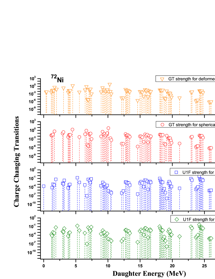
Figure 1: Allowed (GT) and unique first-forbidden (U1F) charge-changing transition strengths calculated in the pn-QRPA(N) model for deformed and spherical cases of ⁷²Ni.

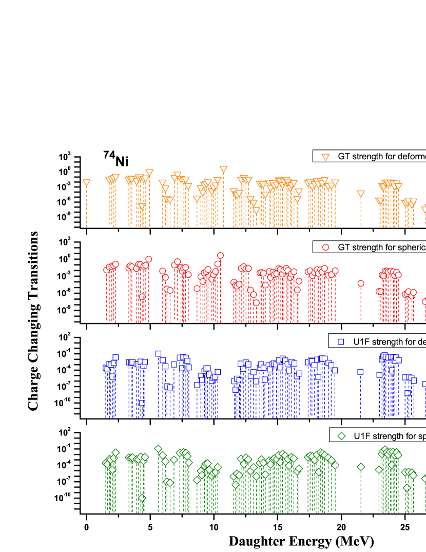
Figure 2: Same as Fig. 1 but for ⁷⁴Ni.

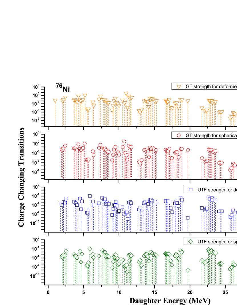
Figure 3: Same as Fig. 1 but for ⁷⁶Ni.

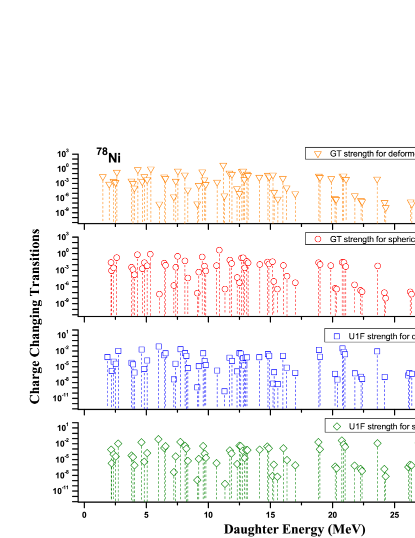
Figure 4: Same as Fig. 1 but for ⁷⁸Ni.

The deformation parameters for the even-even isotopes of Ni used in both pn-QRPA(WS) and pn-QRPA(N) models are shown in Table 3. In order to study the effect of deformation in Nilsson calculation, we performed two sets of calculation within the pn-QRPA(N) model. In the first case the deformation parameter was taken as zero and in the second case the deformation was taken from Table 3. The resulting charge-changing transitions both for allowed and U1F transitions are shown in Figs. 1-4 for ⁷²Ni, ⁷⁴Ni, ⁷⁶Ni and ⁷⁸Ni, respectively. The small value of deformation does not appreciably change the calculated strength distributions except for a few states in the low-lying energy region. The calculated allowed GT and U1F $\beta$-decay rates for the spherical and deformed cases were almost the same. Only at high stellar temperatures (T${}_{9}\geq$ 10) did the decay rate for the deformed case increase by around 10$\%$ as against those cases where we treated the nuclei as spherical.

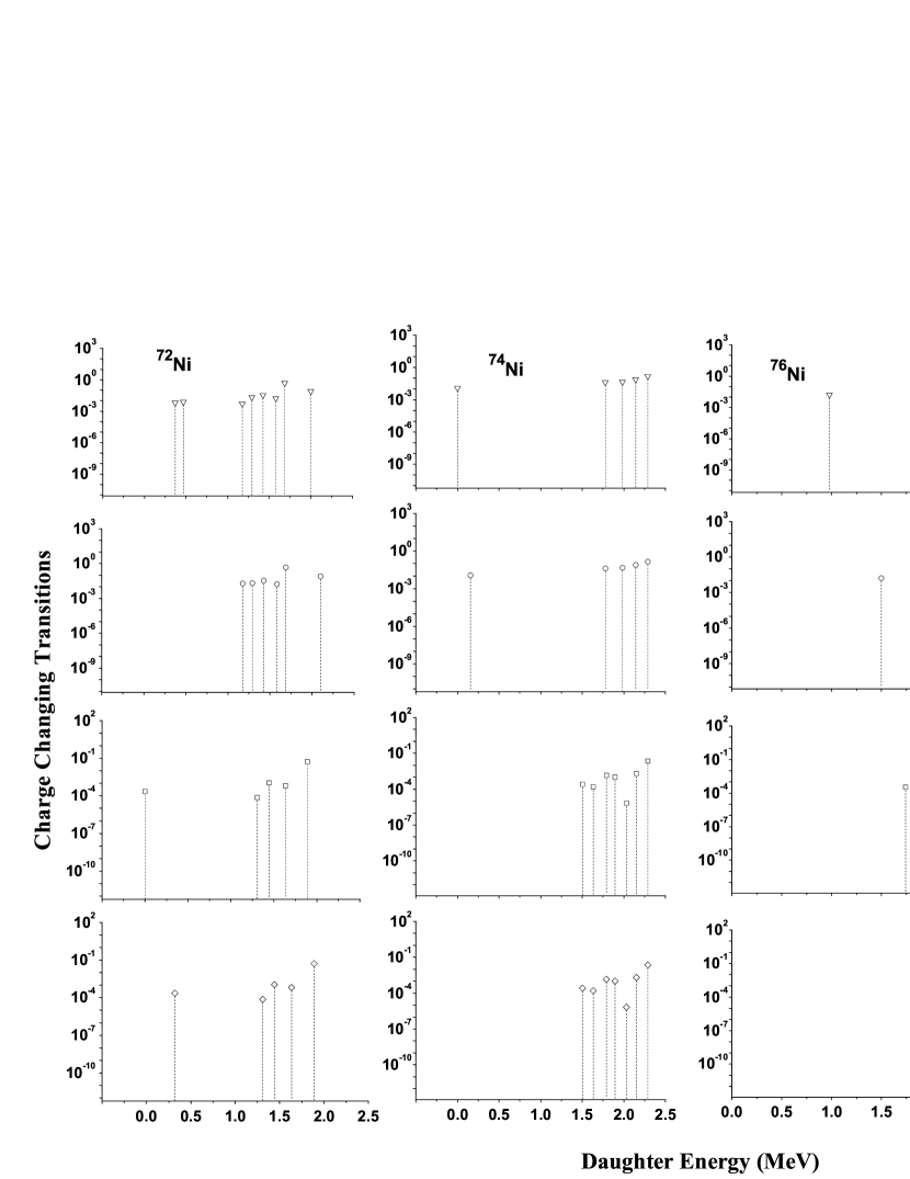
Figure 5: Allowed (GT) and unique first-forbidden (U1F) charge-changing transition strengths calculated in the pn-QRPA(N) model before and after insertion of experimental data.

Insertion of experimental data in the pn-QRPA(N) model deserves special mention. If the original calculated charge-changing strength distribution differs considerably from those after insertion of experimental data then it undermines the predictive power of the pn-QRPA(N) model. Fig. 5 shows the calculated strength distributions before and after insertion of experimental data both for allowed GT and U1F transitions. In case of allowed GT strength distribution for ⁷²Ni, the first calculated state is fragmented into three states (two of which are placed at experimentally measured levels). In other cases there is displacement of first few energy levels within 500 keV (which is roughly the uncertainty in calculation of energy eigenvalues in the pn-QRPA(N) model). Further there are no experimental insertions beyond 2.5 MeV in daughter energy in all nickel isotopes. The predictive power of the pn-QRPA(N) model gets better for shorter half-lives, that is, with increasing distance from line of stability Hir93 .

The allowed GT $\beta$-decay half-lives of nickel isotopes calculated within the pn-QRPA formalism are shown in Table 4. The calculated half-lives are also compared with experimental data. The recent atomic mass evaluation data of Ref. Aud12 have been used for experimental half-lives values. The calculated half-lives of Möller et al from Moe97 are also shown in comparison which uses the deformation of nucleus and folded-Yukawa single-particle potential. It may be concluded that QRPA calculation of Möller et al. improves as the nucleus becomes more neutron-rich. It can be seen that the pn-QRPA(N) and pn-QRPA(WS-DSM) models calculate half-lives in better agreement with the measured half-lives.

The FF contributions to the total calculated half-lives are shown in Table 5. Here we present the GT+U1F calculation of half-lives in the pn-QRPA(N) model and the GT+rank0+rank1+rank2 half-lives calculation using the pn-QRPA(WS-SSM) model. We are currently working on rank1 and rank 2 calculation of half-lives in the pn-QRPA(N) model. Calculation of FF contributions in pn-QRPA(WS-SPM) and pn-QRPA(WS-DSM) models would also be taken as a future assignment. Table 5 shows that the calculated half-lives get appreciably smaller and in better agreement with measured half-lives when the U1F contribution is added in the pn-QRPA(N) model. Likewise, but to a smaller extent, the half-lives get smaller once the FF contributions are added in the pn-QRPA(WS-SSM) model. Contribution of U1F rates to total $\beta$-decay half-lives in the pn-QRPA(N) model is 19.7$\%$, 24.0$\%$, 18.5$\%$ and 17.5$\%$ for ⁷²Ni, ⁷⁴Ni, ⁷⁶Ni and ⁷⁸Ni, respectively. Calculated half-lives of Bor05 using the DF3 + CQRPA model (which includes the FF contribution) can also be seen in Table 5. The DF3 + CQRPA results get in better agreement with experimental data as $N$ (neutron number) increases. It is concluded that pn-QRPA(N) emerges as the best model and has overall excellent agreement with experimentally determined half-lives of Ni isotopes. It is also expected to give reliable results for nuclei close to neutron-drip line for which no experimental data is available.

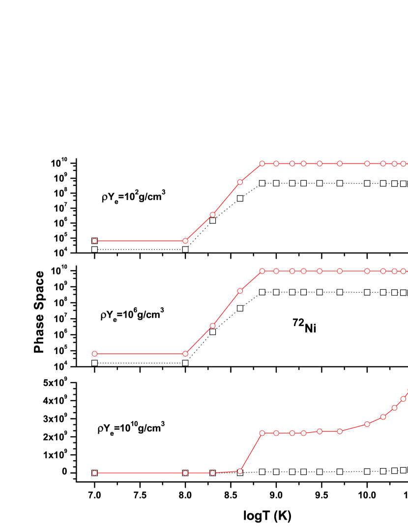
Figure 6: Comparison of calculated phase space for allowed and U1F transitions for ⁷²Ni as a function of stellar temperatures and densities.

The phase space calculation for allowed and U1F transitions, as a function of stellar temperature and density, for the neutron-rich nickel isotope (⁷²Ni) is shown in Fig. 6. The phase space is calculated at selected density of 10² g/cm³, 10⁶ g/cm³ and 10¹⁰ g/cm³ (corresponding to low, intermediate and high stellar densities, respectively) and stellar temperature T₉ = 0.01 - 30 given in logarithmic scale. It can be seen from Fig. 6 that, for low and intermediate stellar densities, the U1F phase space is a factor 4 bigger than the allowed phase space at low temperatures. As stellar temperature soars the phase space for U1F transitions is around a factor 25 bigger. For high densities the phase space is essentially zero at small stellar temperature T${}_{9}\sim$ 0.01 and increases with increasing temperatures. At high density the U1F phase space is around a factor 25 bigger at high temperatures. It can be further be noted from Fig. 6 that for low and intermediate stellar densities the phase space increases by 4-8 orders of magnitude as the stellar temperature goes from T₉ = 0.01 to 1. Moreover the calculated phase space remains same as stellar temperature soars from T₉ = 1 to 30. At a fixed stellar temperature, the phase space remains the same as the core stiffens from low to intermediate stellar density. This is because the electron distribution function at a fixed temperature changes appreciably only once the stellar density exceeds 10⁷ g/cm³. This happens because of an appreciable increase in the calculated Fermi energy of the electrons once the stellar density reaches 10⁷ g/cm³ and beyond. As the stellar core becomes more and more dense the phase space decreases. Phase space calculations of remaining isotopes namely ^74,76,78Ni shows a similar trend. When the nickel isotopes becomes more and more neutron-rich, the phase space enhancement for U1F transitions decreases but still is bigger than the phase space for allowed transitions and lead to a a significant U1F contribution to the total $\beta$–decay rates.

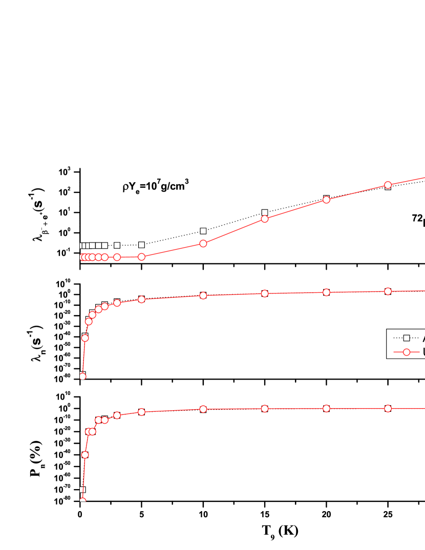
Figure 7: Allowed (GT) and unique first-forbidden (U1F) $\beta$-decay $\&$ positron capture rates (upper panel) and energy rates of neutron (middle panel) for ⁷²Ni as a function of temperature for selected density of 10⁷g.cm^-3. Shown also are the probabilities of $\beta$-delayed neutron emissions (bottom panel).

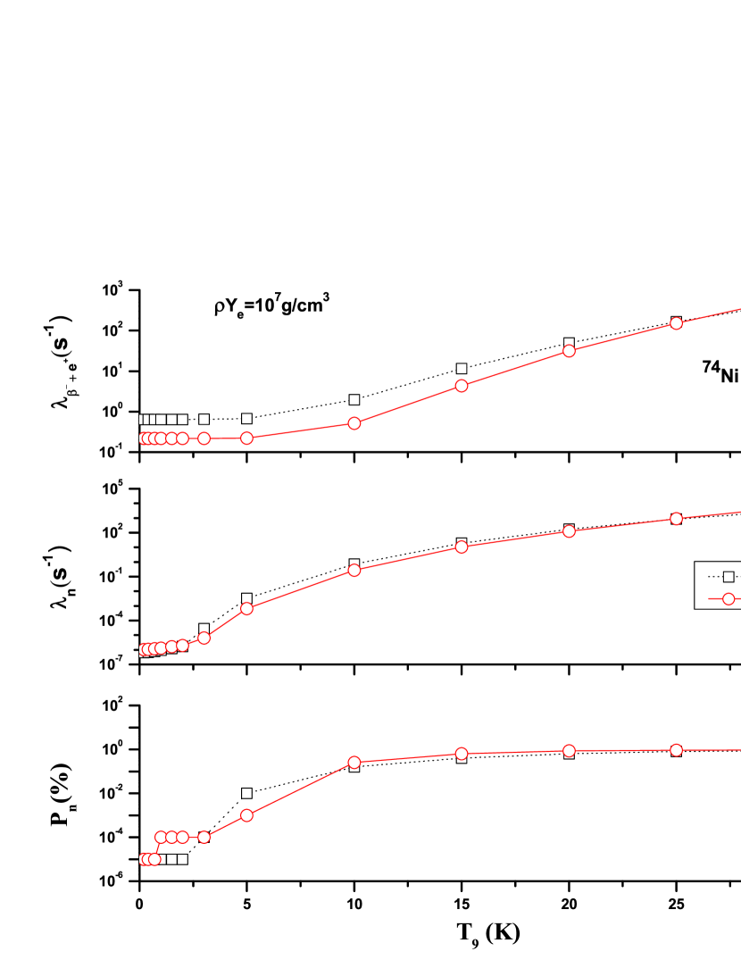
Figure 8: Same as Fig. 7 but for ⁷⁴Ni.

The stellar $\beta$-decay and positron capture rates are calculated for nickel isotopes (^72,74,76,78Ni) in density range of 10-10¹¹g/cm³ and temperature ranging from 0.01 $\leq$ T₉ $\leq$ 30. Figs. 7 - 10 show three panels graph in which the upper panel is depicting pn-QRPA calculated allowed and U1F $\beta$-decay+positron capture rates of Ni isotopes at a stellar density of 10⁷ g/cm³. It is to be noticed that contribution from all excited states are included in the final calculation of all rates. The allowed rates, for intermediate density, in upper panel of Fig. 7, are roughly a factor four bigger at low temperatures and around a factor two smaller at T₉ = 30 as compared to U1F rates. In order to understand this behavior, one has to calculate the relative contribution of $\beta$-decay and positron capture rates to the total rates both for allowed GT and U1F cases. Table 6 shows the relative contribution for allowed GT rates for nickel isotopes as a function of stellar temperature at a fixed density of 10⁷ g/cm³ in the pn-QRPA(N) model. For low stellar temperatures it is a safe assumption to neglect the positron capture rates when compared with the $\beta$-decay rates . At high temperatures ($kT>$ 1 MeV), positrons appear via electron-positron pair creation and their capture rates exceed the competing $\beta$-decay rates by a factor of 25 at T₉ = 30 for the case of ⁷²Ni. Roughly same trend is seen for ^74,76,78Ni. Table 7 shows a similar comparison for the case of U1F rates. Here one notes that, at high stellar temperatures, the contribution of positron capture rates is much bigger to the total rates as against those of allowed GT rates (e.g. for the case of ⁷²Ni the positron capture rates is around three orders of magnitude bigger than the $\beta$-decay rates at T₉ = 30). For ⁷⁴Ni, upper panel of Fig. 8 shows that, at low temperatures, the allowed rates are a factor three bigger and as temperature soars to T₉ = 30, the U1F rates surpass the allowed rates. For the case of ⁷⁶Ni and ⁷⁸Ni, the allowed rates are bigger than the corresponding U1F rates for all temperatures. The relative contributions of allowed and U1F $\beta$-decay and positron capture rates as well as phase space calculations provide the necessary explanation

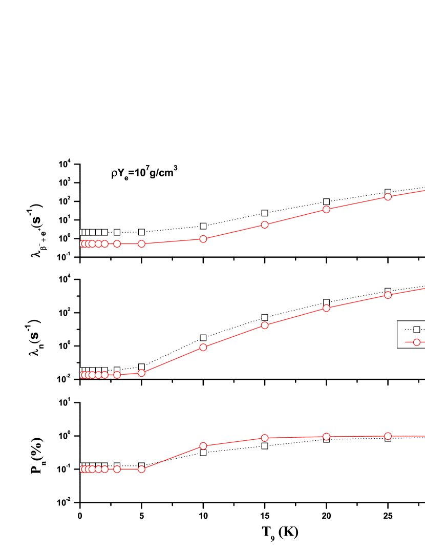
Figure 9: Same as Fig. 7 but for ⁷⁶Ni.

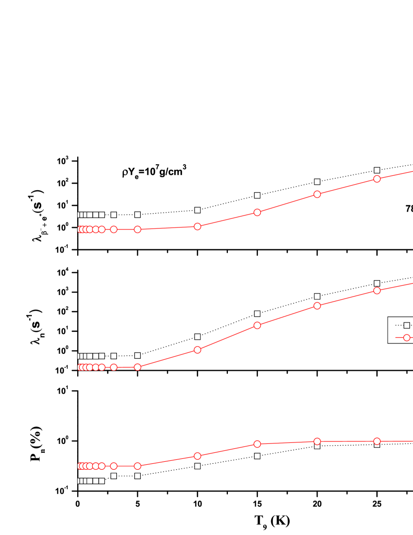
Figure 10: Same as Fig. 7 but for ⁷⁸Ni.

The second panel in Fig. 7 - 10 depicts the behavior of the calculated stellar rates of $\beta$-delayed neutron emission for Ni isotopes through allowed and U1F transitions. All rates are given in units of $MeV.s^{-1}$. The rates are calculated for intermediate density and temperature range of 0.01 $\leq$ T₉ $\leq$ 30. In Fig. 7 (⁷²Ni) the calculated rates of $\beta$-delayed neutron emission for allowed GT are about two order of magnitude bigger than U1F at low temperatures. At high temperatures the U1F rates are 3 times bigger. For the case of ⁷⁴Ni (Fig. 8) the U1F neutron emission rates are roughly twice that of allowed at low temperatures. As temperature increases the allowed rates surpass the U1F rates. At T₉ = 30, once again the U1F rates are twice the allowed rates. The scenario gets interesting for the cases of ⁷⁶Ni and ⁷⁸Ni (see middle panels of Fig. 9 and Fig. 10, respectively) where the neutron emission rates from allowed transitions are around a factor 1.5 - 4 bigger than the U1F rates for all temperature range. The total rates are a product of phase space and nuclear matrix elements. Whereas numerical techniques were used for the calculation of phase space integrals, we again re-iterate that all nuclear matrix elements were calculated in a microscopic fashion which is a distinguishing feature of our work.

The $\beta$-delayed neutron emission probabilities ($P$_n) are very important for a good description of both the separation energies of the neutron (S_n) and the $\beta$ strength functions within the Q_β window. The $\beta$-delayed neutron emission probabilities for Ni isotopes are presented in this paper for the first time (see bottom panels of Figs. 7 - 10). Borzov Bor05 did comment on the $A$ dependence of the calculated $P$_n values for Ni isotopes. We notice a similar behavior of increasing values of $P$_n verses mass number $A$ in Figs. 7 - 10. Borzov further noted that the increase in $\beta$-delayed neutron emission probability for Ni isotopes with A $\leq$ 79 was entirely due to relatively low-energy GT and FF $\beta$-decays. For all cases (^72,74,76,78Ni) the $\beta$-delayed neutron emission probabilities due to U1F transitions are bigger than those due to allowed GT transitions at high temperatures (T${}_{9}\geq$ 10). At low temperatures the emission probabilities are much too smaller for ^72,74Ni and becomes effective only for the neutron-richer isotopes ^76,78Ni.

4 Conclusions

The contribution of FF transitions to total $\beta$-decay becomes significant for neutron-rich isotopes. We used different versions of the pn-QRPA model using two different single-particle potentials. We used the Woods-Saxon potential to calculate allowed GT transitions for isotopes of nickel using the pn-QRPA(WS-SSM), pn-QRPA(WS-SPM) and pn-QRPA(WS-DSM) models. The calculated half-lives showed pn-QRPA(WS-DSM) to be the better model. Results of pn-QRPA(WS-SPM) model were not very encouraging. The pn-QRPA(WS-SSM) model was later used to calculate the FF contribution which led to a better agreement of the calculated half-lives with the measured data. The pn-QRPA(N) model employed the Nilsson potential and was used to calculate allowed GT and GT+U1F half-lives. The agreement with experimental data was the best for the pn-QRPA(N) model. The FF inclusion improved the overall comparison of calculated terrestrial $\beta$-decay half-lives in the pn-QRPA(WS-SSM) model. Likewise, and more significantly, the UIF contribution improved the pn-QRPA(N) calculated half-lives. The DF3 + CQRPA calculation was in good agreement with experimental data for heavier isotopes and allowed GT calculation by Möller and collaborators was way too big for ^72,74,76Ni but was in somewhat better agreement for ⁷⁸Ni.

It was also shown that the U1F phase space has a sizeable contribution to the total phase space at stellar temperatures and densities. It was shown that, for a particular element, the U1F phase space gets amplified with increasing neutron number. For the case of pn-QRPA(N) model the U1F rates contribute roughly 20$\%$ to the total $\beta$-decay half-lives. It is expected that contribution of FF transition may increase further with increasing neutron number. However there is a need to study many more neutron-rich nuclei in order to authenticate this claim which we would like to take as a future assignment. The microscopic calculation of U1F $\beta$-decay rates, presented in this work, could lead to a better understanding of the nuclear composition and $Y_{e}$ in the core prior to collapse and collapse phase. The energy rates of $\beta$-delayed neutrons and probability of $\beta$-delayed neutron emissions were also calculated in stellar matter.

The reduced $\beta$-decay half-lives calculated in this work bear consequences for nucleosynthesis problem and site-independent $r$-process calculations. Our findings might result in speeding-up of the $r$-matter flow relative to calculations based on half-lives calculated from only allowed GT transitions. The effects of shorter half-lives resulted in shifting of the third peak of the abundance of the elements in the $r$-process toward higher mass region Suz12 . The allowed and U1F $\beta$-decay rates on Ni isotopes were calculated on a fine temperature-density grid, suitable for simulation codes, and may be requested as ASCII files from the corresponding author.

Acknowledgments

J.-U. Nabi would like to acknowledge the support of the Higher Education Commission Pakistan through the HEC Project No. 20-3099.

Table 1: Calculated GT strength for ^72,74,76,78Ni using pn-QRPA(WS-DSM, WS-SSM, WS-SPM) models.

A	Ej		Ej		Ej
	(MeV)	$|\langle 1_{j}^{+}||M_{GT-}^{DSM}||0^{+}_{g.s}\rangle|^{2}$	(MeV)	$|\langle 1_{j}^{+}||M_{GT-}^{SSM}||0^{+}_{g.s}\rangle|^{2}$	(MeV)	$|\langle 1_{j}^{+}||M_{GT-}^{SPM}||0^{+}_{g.s}\rangle|^{2}$
	0.01	6.70$\times 10^{-6}$	0.31	1.40$\times 10^{-3}$	0.88	4.90$\times 10^{-4}$
72	0.02	1.20$\times 10^{-5}$
	0.22	5.90$\times 10^{-3}$
	0.07	6.10$\times 10^{-4}$	0.28	9.80$\times 10^{-2}$	0.12	2.70$\times 10^{-3}$
74	0.13	3.30$\times 10^{-3}$	0.43	3.70$\times 10^{-3}$	1.09	2.30$\times 10^{-3}$
	0.57	1.20$\times 10^{-4}$
	0.50	1.20$\times 10^{-4}$	0.32	1.04$\times 10^{-1}$	0.28	4.50$\times 10^{-2}$
	0.60	1.40$\times 10^{-4}$	1.44	6.50$\times 10^{-2}$	0.78	2.30$\times 10^{-2}$
76	0.75	2.30$\times 10^{-4}$	1.57	1.40$\times 10^{-3}$	1.91	8.20$\times 10^{-3}$
	0.85	2.90$\times 10^{-4}$
	0.86	3.00$\times 10^{-4}$
	1.00	9.90$\times 10^{-5}$	0.81	3.70$\times 10^{-2}$	0.49	5.30$\times 10^{-4}$
78	1.40	2.50$\times 10^{-4}$	0.91	2.07$\times 10^{-3}$	0.89	1.30$\times 10^{-2}$
	1.70	5.50$\times 10^{-4}$

Table 2: Calculated GT strengths (rank0, rank1 and rank2 transitions) for ^72,74,76,78Ni using the pn-QRPA (WS-SSM) model.

A	Ej		Ej		Ej
	(MeV)	$|\langle 0_{j}^{-}||M_{\beta-}^{0}||0^{+}\rangle|^{2}$	(MeV)	$|\langle 1_{j}^{+}||M_{\beta-}^{1}||0^{+}\rangle|^{2}$	(MeV)	$|\langle 2_{j}^{+}||M_{\beta-}^{2}||0^{+}\rangle|^{2}$
72	2.01	1.80$\times 10^{-4}$	0.95	3.4$\times 10^{-4}$	2.15	2.40$\times 10^{-2}$
74	1.76	2.30$\times 10^{-4}$	0.18	3.3$\times 10^{-4}$	0.03	8.20$\times 10^{-3}$
76	0.19	3.10$\times 10^{-4}$	1.47	9.50$\times 10^{-4}$	1.49	6.70$\times 10^{-3}$
78	1.63	5.90$\times 10^{-4}$	0.26	3.10$\times 10^{-4}$	0.21	6.80$\times 10^{-3}$

Table 3: Deformation parameters used in the pn-QRPA(N) and pn-QRPA(WS-DSM) calculations.

A	$\delta$
72	0.00896
74	0.01583
76	0.01037
78	0.00340

Table 4: Allowed GT $\beta$-decay half-lives (in seconds) for Ni isotopes calculated using the pn-QRPA(N) and pn-QRPA(WS-DSM, WS-SSM, WS-SPM) models, in comparison with experimental data Aud12 and those by Ref. Moe97 .

		pn-QRPA	pn-QRPA	pn-QRPA	pn-QRPA
A	Exp	(N)	(WS-DSM)	(WS-SSM)	(WS-SPM)	Möller
		(GT)	(GT)	(GT)	(GT)	(GT)
72	1.57	2.50	1.04	1.12	12.6	42.7
74	0.68	0.98	0.71	0.35	1.23	26.8
76	0.24	0.29	0.20	1.07	0.18	3.07
78	0.14	0.17	0.11	0.16	0.12	0.22

Table 5: Total $\beta$-decay half-lives (in seconds) for Ni isotopes calculated using the pn-QRPA(N) and pn-QRPA(WS-SSM) models for allowed plus first-forbidden transitions, in comparison with experimental data Aud12 and the DF3 + CQRPA Bor05 calculation.

		pn-QRPA	pn-QRPA	pn-QRPA	pn-QRPA
A	Exp	(N)	(WS-SSM)	(WS-SSM)	(WS-SSM)	DF3+CQRPA
		(GT+rank2)	(GT+rank2)	(GT+rank0,1,2)	(GT+rank0)	(GT+rank0)
72	1.57	2.01	1.12	1.09	1.11	1.33
74	0.68	0.74	0.34	0.32	0.35	0.53
76	0.24	0.24	1.01	0.89	1.03	0.26
78	0.14	0.14	0.15	0.15	0.15	0.13

Table 6: Calculated $\beta^{-}$-decay rates for allowed GT transitions (in units of s^-1) and ratio of $\beta^{-}$-decay to positron capture rates on ^72,74,76,78Ni at stellar density of 10⁷g/cm³ in the pn-QRPA(N) model. T₉ represents the temperature in 10⁹K.

	72Ni		74Ni		76Ni		78Ni
T9	$\lambda_{\beta^{-}}$	R($\beta^{-}/e^{+}$)	$\lambda_{\beta^{-}}$	R($\beta^{-}/e^{+}$)	$\lambda_{\beta^{-}}$	R($\beta^{-}/e^{+}$)	$\lambda_{\beta^{-}}$	R($\beta^{-}/e^{+}$)
1	2.3$\times 10^{-1}$	1.4$\times 10^{11}$	6.3$\times 10^{-1}$	2.8$\times 10^{11}$	2.1$\times 10^{0}$	5.0$\times 10^{11}$	3.7$\times 10^{0}$	7.7$\times 10^{11}$
3	2.4$\times 10^{-1}$	8.2$\times 10^{3}$	6.5$\times 10^{-1}$	1.7$\times 10^{4}$	2.2$\times 10^{0}$	3.2$\times 10^{4}$	3.7$\times 10^{0}$	5.0$\times 10^{4}$
5	2.6$\times 10^{-1}$	8.6$\times 10^{1}$	6.7$\times 10^{-1}$	1.9$\times 10^{2}$	2.3$\times 10^{0}$	3.6$\times 10^{2}$	3.8$\times 10^{0}$	5.6$\times 10^{2}$
10	8.7$\times 10^{-1}$	2.4$\times 10^{0}$	1.6$\times 10^{0}$	4.3$\times 10^{0}$	4.1$\times 10^{0}$	7.3$\times 10^{1}$	5.5$\times 10^{0}$	1.1$\times 10^{1}$
30	2.1$\times 10^{1}$	4.0$\times 10^{-2}$	2.6$\times 10^{1}$	6.0$\times 10^{-2}$	7.2$\times 10^{1}$	9.3$\times 10^{-2}$	1.3$\times 10^{2}$	1.4$\times 10^{-1}$

Table 7: Same as Table 6 but for U1F transitions.

	72Ni		74Ni		76Ni		78Ni
T9	$\lambda_{\beta^{-}}$	R($\beta^{-}/e^{+}$)	$\lambda_{\beta^{-}}$	R($\beta^{-}/e^{+}$)	$\lambda_{\beta^{-}}$	R($\beta^{-}/e^{+}$)	$\lambda_{\beta^{-}}$	R($\beta^{-}/e^{+}$)
1	6.3$\times 10^{-2}$	5.8$\times 10^{11}$	2.1$\times 10^{-1}$	1.7$\times 10^{12}$	5.1$\times 10^{-1}$	2.8$\times 10^{12}$	8.2$\times 10^{-1}$	4.1$\times 10^{12}$
3	6.4$\times 10^{-2}$	1.5$\times 10^{4}$	2.1$\times 10^{-1}$	4.6$\times 10^{4}$	5.1$\times 10^{-1}$	8.1$\times 10^{4}$	8.2$\times 10^{-1}$	1.2$\times 10^{5}$
5	6.5$\times 10^{-2}$	9.8$\times 10^{1}$	2.2$\times 10^{-1}$	3.0$\times 10^{2}$	5.2$\times 10^{-1}$	5.6$\times 10^{2}$	8.2$\times 10^{-1}$	8.7$\times 10^{2}$
10	1.0$\times 10^{-1}$	5.2$\times 10^{-1}$	3.5$\times 10^{-1}$	2.0$\times 10^{0}$	7.7$\times 10^{-1}$	4.4$\times 10^{0}$	9.7$\times 10^{-1}$	7.1$\times 10^{0}$
30	5.0$\times 10^{-1}$	5.4$\times 10^{-4}$	1.6$\times 10^{0}$	2.8$\times 10^{-3}$	5.3$\times 10^{0}$	8.4$\times 10^{-3}$	1.1$\times 10^{1}$	1.9$\times 10^{-2}$

References

- (1) J. Dobaczewski et al., Phys. Rev. Lett., 72, 981 (1994).
- (2) K. -L. Kratz et al., Astrophys. J., 403, 216 (1993).
- (3) E. M. Burbidge, G. M. Burbidge, W. A. Fowler, F. Hoyle, Rev. Mod. Phys., 29, 547 (1957).
- (4) A. G. W. Cameron, Pub. Astron. Soc. Pacific, 69, 201 (1957).
- (5) J. J. Cowan, F. -K. Thielemann, and J. W. Truran, Phys. Rep., 208, 267 (1991).
- (6) S. E. Woosley, G. J. Mathews, J. R. Wilson, R. D. Hoffman and B. S. Meyer, Astrophys. J., 433, 229 (1994).
- (7) J. Cooperstein and J. Wambach, Nucl. Phys. A, 420, 591 (1984).
- (8) J.-U. Nabi and S. Stoica, Astro. Space Sci., 349, 843 (2013).
- (9) Q. Zhi, E. Caurier, J. J. Cuenca-García, K. Langanke, G. Martínez-Pinedo and K. Siega, Phys. Rev. C, 87, 025803 (2013).
- (10) I. Borzov, Nucl. Phys. A., 777, 645 (2006).
- (11) H. Homma, E. Bender, M. Hirsch, K. Muto, H. V. Klapdor-Kleingrothaus and T. Oda, Phys. Rev. C, 54, 2972 (1996).
- (12) J. A. Halbleib, R. A. Sorensen, Nucl. Phys. A., 98, 542 (1967).
- (13) J.-U. Nabi and H. V. Klapdor-Kleingrothaus, Eur. Phys. J. A., 5, 337 (1999).
- (14) J.-U. Nabi and H. V. Klapdor-Kleingrothaus, At. Data Nucl. Data Tables, 71, 149 (1999).
- (15) J.-U. Nabi and H. V. Klapdor-Kleingrothaus, At. Data Nucl. Data Tables, 88, 237 (2004).
- (16) S. I. Gabrakov and A. A. Kuliev, JINR P4, 5003, 1-10 (1970).
- (17) H. A. Aygör, Phd Thesis, Suleyman Demirel University,Isparta, Turkey, (2002).
- (18) C. Selam, A. Kucukbursa, H. Bircan, H. A. Aygör, T. Babacan, I. Maras and A. Kokce, Turk. J. of Phys., 27, 187-193, (2003).
- (19) C. Selam, T. Babacan, H. A. Aygör, H. Bircan, A. Kucukbursa and I. Maras, Math. and Comp. App.,9, 1, 79-90, (2004).
- (20) N. Cakmak, S. Unlu, C. Selam et al., Pram. J. Phys., 75,4, 649-663, (2010).
- (21) N. Cakmak, S. Unlu, C. Selam, Phys. Atm. Nuc., 75, 8 (2012).
- (22) A. Bohr and B. R. Mottelson, Nuclear Structure, (Benjamin, New York, 1969).
- (23) N. Cakmak, K. Manisa, S. Unlu and C. Selam, Pram. J. Phys. 74, 541 (2010).
- (24) K. Muto, E. Bender, T. Oda, H. V. Klapdor-Kleingrothaus, Z. Phys. A., 341, 407 (1992).
- (25) J. Krumlinde and P. Möller, Nucl. Phys. A, 417, 419 (1984).
- (26) P. Möller and J. Randrup, Nucl. Phys. A, 514, 1 (1990).
- (27) E. Bender, K. Muto and H. V. Klapdor, Phys. Lett. B., 208, 53 (1988).
- (28) A. Staudt, E. Bender, K. Muto and H. V. Klapdor, Z. Phys. A, 334, 47 (1989).
- (29) A. Staudt, E. Bender, K. Muto and H. V.Klapdor-Kleingrothaus, At. Data. Nucl. Data Tables, 44, 79 (1990).
- (30) J. Suhonen, T. Taigel and A. Faessler, Nucl. Phys. A, 486, 91 (1988).
- (31) M. Hirsch, A. Staudt, K. Muto and H. V. Klapdor-Kleingrothaus, Nucl. Phys. A, 535, 62 (1991).
- (32) M. Hirsch, A. Staudt, K. Muto and H. V. Klapdor-Kleingrothaus, At. Data Nucl. Data Tables, 53, 165 (1993).
- (33) J.-U. Nabi, Adv. Space Res., 46, 1191 (2010)
- (34) J.-U. Nabi, Adv. Space Res., 48, 985 (2011).
- (35) J.-U. Nabi, Astro. Space Sci., 331, 537 (2011).
- (36) J.-U. Nabi, Eur. Phys. J. A., 48, 84 (2012).
- (37) J.-U. Nabi and C. W. Johnson, J. Phys. G, 40, 065202 (2013)
- (38) O. Civitarese, F. Krmpotic and O. A. Rosso, Nucl. Phys. A, 453, 45 (1986).
- (39) P. Möller, B. Pfeiffer and K.-L. Kratz, Phys. Rev. C, 67, 055802 (2003).
- (40) J.-U. Nabi, N. Cakmak and Z. Iftikhar, Phys. Scr., 90, 115301 (2015).
- (41) P. Möller and J. R. Nix, At. Data Nucl. Data Tables, 26, 165 (1981).
- (42) G. Audi, M. Wang, A.H. Wapstra, F.G. Kondev, M. MacCormick, X. Xu and B. Pfeiffer, Chin. Phys. C, 36 1287 (2012); M. Wang, G. Audi, A.H. Wapstra, F.G. Kondev, M. MacCormick, X. Xu and B. Pfeiffer B, Chin. Phys. C, 36 1603 (2012).
- (43) N. B. Gove, M. J. Martin, At. Data Nucl. Data Tables, 10, 205 (1971).
- (44) P. Möller, J. R. Nix and K. -L. Kratz, At. Data Nucl. Data Tables, 66, 131 (1997).
- (45) I. N. Borzov, Phys. Rev. C, 71, 065801 (2005).
- (46) T. Suzuki, T. Yoshida, T. Kajino and T. Otsuka, Phys. Rev. C, 85, 015802 (2012).