Gamow-Teller strength distributions and neutrino energy loss rates due to chromium isotopes in stellar matter

Abstract

Gamow-Teller transitions in isotopes of chromium play a consequential role in the presupernova evolution of massive stars. $\beta$-decay and electron capture rates on chromium isotopes significantly affect the time rate of change of lepton fraction ($\dot{Y_{e}}$). Fine-tuning of this parameter is one of the key for simulating a successful supernova explosion. The (anti)neutrinos produced as a result of electron capture and $\beta$-decay are transparent to stellar matter during presupernova phases. They carry away energy and this result in cooling the stellar core. In this paper we present the calculations of Gamow-Teller strength distributions and (anti)neutrino energy loss rates due to weak interactions on chromium isotopes of astrophysical importance. We compare our results with measured data and previous calculations wherever available.

Keywords neutrino energy loss rates; Gamow-Teller transitions; pn-QRPA theory; stellar evolution; core-collapse.

1 Introduction

Elements heavier than helium are synthesized in the stars via fusion chain reactions during the course of stellar evolution. Once the nucleosynthesis process cooks iron (⁵⁶Fe), the binding energy per nucleon curve prohibits any further production of energy by nuclear fusion. When the iron core, formed in the center of a massive star, grows by silicon shell burning to a mass around 1.5 M_⊙, the electron degeneracy pressure required to counter the enormous self-gravity force of the star is reduced and the core becomes unstable. This starts what is normally termed as core-collapse supernova, in the course of which the star explodes and the parts of heavy-element core and its outer shells are ejected into the intersteller medium. In addition to disseminating nuclei formed during stellar evolution, supernova play a key role in synthesizing additional heavy elements. These elements (heavier than iron) are thought to be formed in the r-process nucleosynthesis and type II supernova explosions are considered to be the most probable site for such neutron-capture processes (Cowan et al., 2004). Thus, a detailed understanding of the explosion mechanism is not only necessary for the fate of a star’s life but also for understanding the very important nucleosynthesis problem which is intricately linked with the microphysics of core collapse.

Since 1934, when Baade and Zwicky (Baade et al., 1934) proposed that a supernova represents the transition of a normal star to a neutron star, scientists have been debating about the details of the mechanism responsible for these spectacular explosions. Unfortunately, the supernova explosion mechanism is still mysterious. To date, core- collapse simulators find it challenging to successfully transform the collapse into an explosion.

Core collapse creates high temperatures ($>$ 1 MeV) and densities ($10^{7}$ g cm${}^{-3}<\rho<$ 10¹⁵ g cm^-3) and produces either a neutron star or black hole. Under such extreme thermodynamic conditions, neutrinos are produced in abundance. The discovery of neutrino burst from SN1987A by the Kamiokande II group (Hirata et al., 1987) and IMB group (Bionta et al., 1987) energized the research on neutrino astrophysics. Neutrinos are considered to play a critical role in our understanding of the dynamics of supernova. They not only provide an essential probe into the core-collapse mechanism, but also probably play an active role in the explosion mechanism. They seem to be mediators of the transfer of energy from the inner core to the outer mantle of the iron core. This energy transfer is thought to transform the collapse into an explosion.

According to our present understanding of the explosion mechanism, the onset of the collapse and infall dynamics are very sensitive to the core entropy and to the lepton to baryon ratio, Y_e (Bethe et al., 1979). These two quantities are mainly determined by weak interaction processes, electron capture and $\beta$-decay. Electron capture on (Fe-peak) nuclei is energetically favorable when electron Fermi energy reaches the nuclear energy scale (energies in the MeV range). This produces neutrinos and reduces the number of electrons available for the pressure support. Many of the nuclei present can also $\beta$-decay, a process which acts in the opposite direction. These weak-interaction mediated reactions affect the overall lepton to baryon ratio of the core and directly influence the collapse dynamics.

At the start of collapse, while densities in the core are $\sim 10^{9}$ g cm^-3, the neutrinos can freely escape the collapsing star and therefore assist in cooling the core to a lower entropy state. As the core density reaches $\rho\sim 10^{12}$ g cm^-3, an important change occurs in the physics of the core collapse. At such high densities, (where neutrino diffusion time becomes larger than the collapse time) (Bethe, 1990) neutrinos feel the pressure of matter and can become trapped in the so-called neutrinosphere, mainly due to elastic scattering with nuclei. After neutrino trapping, the collapse proceeds essentially homologously (Goldreich et al., 1980), until nuclear densities, $\rho\sim 10^{14}$ g cm^-3, are reached. The homologous core decelerates and bounces in response to the increased nuclear matter pressure. This drives a shock wave into the outer core. If the shock were to propagate outward without stalling, we would have what is called prompt-shock mechanism. However, it appears as if the energy available to the shock is not sufficient, as it loses energy in dissociating heavy nuclei that pass through it as it propagates outward. The shock loses additional energy due to neutrino emission (mainly non-thermal) leading to a standing shock. This stalled shock is thought to be revived by what has become known as the delayed-shock mechanism, originally proposed by Wilson and Bethe (Bethe et al., 1985). The success of this explosion mechanism mainly depends on the cross sections for neutrino capture on nucleons, the neutrino production rates, the details of the neutrino transport, neutrino cooling rates, convection behind the stalled shock, and other factors, many of which are not known with certainty. Depending on these ingredients, simulations of the delayed shock mechanism yielded successful explosions in some cases (Herant et al., 1994; Freher et al., 2000), while they failed in some of the other cases (Buras et al., 2003)-(Thompson et al., 2003).

After core bounce, $\sim 10^{53}$ ergs of energy (Balantekin et al., 2003) is released from the cooling proto-neutron star in the form of neutrinos and antineutrinos of all 3 flavours (electron, muon and tau). Only $1\%$ of this energy needs to be absorbed behind the shock to generate the $\sim 10^{51}$ ergs of energy associated with the explosion. Simulating a $1\%$ effect is indeed a challenging task faced by astrophysicists all around the globe. Neutrinos while propagating through the proto-neutron star interact with the protons, neutrons and electrons in this central object via absorption and scattering. These neutrinos play a vital role in our understanding of the microphysics of the supernova. They provide information concerning the neutronization due to electron capture, the formation, stalling, revival and propagation of the shock wave and the cooling phase. Electron capture rates and associated neutrino cooling rates (as a function of stellar temperature, density and Fermi energy) are important input parameters for modeling the dynamics and supernova collapse phase of massive stars (Strother et al., 2009). A reliable and microscopic calculation of neutrino loss rates and capture rates has thus become a topic of interest for core-collapse simulators all around the world.

Fuller, Fowler, and Newman (FFN) (Fuller et al., 1980, 1982) were the first who performed a comprehensive calculation of stellar weak rates including the capture rates, neutrino energy loss rates and decay rates for a wide range of density and temperature. The calculation was done for 226 nuclei in the mass range $21\leq A\leq 60$. FFN work was later extended by Aufderheide et al. (Aufderheide et al., 1994) for heavier nuclei with $A>60$. Since then theoretical efforts were focused on the microscopic calculations of capture rates of iron-regime nuclide. The proton-neutron quasi particle random phase approximation theory (pn-QRPA) (Nabi et al., 1999) and large-scale shell model (Langanke et al., 2000) were used largely for the microscopic calculation of weak interaction rates in stellar environment.

Weak interaction rates for 709 nuclei with A = 18 to 100 in stellar matter using the pn-QRPA theory were calculated by Nabi and Klapdor  (Nabi et al., 1999). These weak interaction rate calculations included decay rates, capture rates, neutrino energy loss rates, gamma heating rates, probabilities of $\beta$-delayed particle emissions and energy rate of these particle emissions (Nabi et al., 1999, 2004). These calculations were later refined using more efficient algorithms, incorporating latest data from mass compilations and experimental values, and by fine-tuning of model parameters (Nabi et al., 2005)-(Nabi et al., 2007). The present work is devoted to a microscopic calculation of Gamow-Teller strength distribution and detailed analysis of the neutrino and antineutrino energy loss rates due to weak-interaction reactions on isotopes of chromium in stellar environment. The neutrino and antineutrino energy loss rates can occur through four different weak-interaction mediated channels: electron and positron captures, and, electron and positron emissions. The neutrinos are produced due to electron captures and positron decays whereas the antineutrinos are produced due to positron captures and electron decays.

Charge-changing transitions normally referred to as Gamow- Teller (GT) transitions play an important role in many astrophysical events in universe. During early stages of collapse many important nuclear processes, such as $\beta$ decays, electron captures, neutrino absorption and inelastic scattering on nuclei, appear. These reactions are mainly governed by GT (and Fermi) transitions. GT transitions for $fp$-shell nuclei are considered very important for supernova physics (Fuller et al., 1980, 1982). The GT transitions, in $fp$-shell nuclei, play decisive roles in presupernova phases of massive stars and also during the core collapse stages of supernovae (specially in neutrino induced processes). At stellar densities $\sim$ 10¹¹ gcm^-3, for $fp$-shell nuclei, the electron chemical potential approaches the same order of magnitude as the nuclear Q-value. Under such conditions, the $\beta$-decay rates are sensitive to the detailed GT distributions. For still higher stellar densities, the electron chemical potential is much larger than nuclear Q-values. Electron capture rates become more sensitive to the total GT strength for such high densities. To achieve a better understanding of these notoriously complex astrophysical phenomena, a microscopic calculation of GT strength distributions is in order.

The GT excitations deal with the spin-isospin degree of freedom and are executed by the $\sigma\tau_{\pm,0}$ operator, where $\sigma$ is the spin operator and $\tau_{\pm,0}$ is the isospin operator in spherical coordinates. The plus sign refers to the GT₊ transitions where a proton is changed into a neutron (commonly referred to as electron capture or positron decay). On the other hand, the minus sign refers to GT_- transitions in which a neutron is transformed into a proton ($\beta$-decay or positron capture). The third component GT₀ is of relevance to inelastic neutrino-nucleus scattering for low neutrino energies and would not be considered further in this manuscript. Total GT_- and GT₊ strengths (referred to as $B(GT)_{-}$ and $B(GT)_{+}$, respectively, in this manuscript) are related by Ikeda Sum Rule as $B(GT)_{-}-B(GT)_{+}=3(N-Z)$, where $N$ and $Z$ are numbers of neutrons and protons, respectively (Ikeda et al., 1963). Given nucleons are treated as point particles and two-body currents are not considered, the model independent Ikeda Sum Rule should be satisfied by all calculations.

Isotopes of chromium are advocated to play an important role in the presupernova evolution of massive stars. The measured data of GT strength in chromium isotopes have been sparse to the best of our knowledge. The decay of ⁴⁶Cr was studied by (Zioni et al., 1972), who used the ³²S(¹⁶O,2n) reaction to produce ⁴⁶Cr. Later Onishi and collaborators (Onishi et al., 2005) observed the $\beta$-decay of ⁴⁶Cr to the 1${}^{+}_{1}$ state at 993 keV excitation energy in ⁴⁶V. The $T=1$ nuclei decay to the $T=0$ and 1⁺ states of daughter nuclei were called favored-allowed GT transitions and possessed a signature small $ft$ value. The experiment was performed at RIKEN accelerator research facility. Two sets of independent measurement of $B(GT)_{-}$ strength for ⁵⁰Cr were also performed. Fujita et al. did a ⁵⁰Cr(³He, $t$)⁵⁰Mn measurement up to 5 MeV in daughter (Fujita et al., 2011). On the other hand Adachi and collaborators (Adachi et al., 2007) were able to perform a high resolution ⁵⁰Cr(³He, $t$)⁵⁰Mn measurement at an incident energy of 140 MeV/nucleon and at 0⁰ for the precise study of GT transitions. The experiment was performed at RCNP, Japan. Owing to high resolution the authors were able to measure $B(GT)_{-}$ strength up to 12 MeV in ⁵⁰Mn. At higher excitations above the proton separation energy, a continuous spectrum caused by the quasifree scattering appeared in the experiment. Nonetheless there was a need to perform more experiments to measure GT transitions in $fp$-shell nuclei. Next-generation radioactive ion-beam facilities (e.g. FAIR (Germany), FRIB (USA) and FRIB (Japan)) are expected to provide us measured GT strength distribution of many more nuclei. It is also expected to observe GT states in exotic nuclei near the neutron and proton drip lines. However simulation of astrophysical events (e.g. core-collapse supernovae) requires GT strength distributions ideally for hundreds of nuclei. As such experiments alone cannot suffice and one has to rely on reliable theoretical estimates for GT strength distributions.

Aufderheide and collaborators (Aufderheide et al., 1994) searched for key weak interaction nuclei in presupernova evolution of massive stars. Phases of evolution, after core silicon burning, were considered and a search was performed for the most important electron capture and $\beta$-decay nuclei for 0.40 $\leq Y_{e}\leq$ 0.50 ($Y_{e}$ is lepton-to-baryon fraction of the stellar matter). The rate of change of $Y_{e}$ during presupernova evolution is one of the keys to generate a successful explosion. As per their calculation, electron captures on ^51-58Cr and $\beta$-decay of ^{53,54,55,56,57,59,60}Cr were found to be of significant astrophysical importance controlling $Y_{e}$ in stellar matter. Later Heger and collaborators (Heger et al., 2001) performed simulation studies of presupernova evolution employing shell model calculations of weak-interaction rates in the mass range A = 45 to 65. Electron capture rates on ^50,51,53Cr were found to be crucial for decreasing the $Y_{e}$ of the stellar matter. Similarly, it was shown in the same study that $\beta$-decay rates of ^53,54,55,56Cr played a significant role in increasing the $Y_{e}$ content of the stellar matter. These and similar studies of presupernova evolution provided us the motivation to perform a detailed study of GT transitions and the (anti)neutrino energy loss rates due to isotopes of chromium. In this work we calculate and study GT distributions of eleven (11) isotopes of chromium, ^50-60Cr, both in the electron capture and $\beta$-decay direction. The (anti)neutrino energy loss rates of these chromium isotopes are also calculated and compared with previous calculations.

The theoretical formalism used to calculate the GT strength distributions and associated (anti)neutrino energy loss rates in the pn-QRPA model is described briefly in the next section. We compare our results with other model calculations and measurements in Section 3. A decent comparison would put more weight in the predictive power of the pn-QRPA model used in this work. It is pertinent to mention again that our calculation includes many neutron-rich and neutron-deficient isotopes of chromium for which no experimental data is available for now. Core-collapse simulators rely heavily on reliable theoretical estimates of the corresponding weak rates in their codes. Section 4 finally summarizes our work and states the main findings of this study.

2 Model Selection and Formalism

GT strength distributions of ^50-60Cr isotopes were calculated by using the proton-neutron quasiparticle random phase approximation (pn-QRPA) model (we refer specially to the calculations by (Staudt et al., 1990; Hirsch et al., 1993)). The QRPA treats the particle-particle ($pp$) and hole-hole amplitudes in a similar way as in particle-hole ($ph$) amplitudes. The QRPA takes into account pairing correlations albeit in a non-perturbative way. Earlier a similar study for calculation of GT transitions for key chromium isotopes, using different pn-QRPA models, was performed (Cakmak et al., 2015). The idea was to find out the best pn-QRPA model to perform the stellar weak interaction rates with the respective model parameters. It was concluded in (Cakmak et al., 2015) that the current pn-QRPA model was indeed the best model that reproduced not only the available experimental data but had the best predictive power for estimate of weak rates of nuclei far away from line of stability. In this paper we use the same model (with same model parameters) to calculate (anti)neutrino cooling rates due to isotopes of chromium.

In this section, we give necessary formalism used in the pn-QRPA models. Detailed formalism may be seen in (Nabi et al., 2004) and is not reproduced here for space consideration.

2.1 The GT Strength Distribution

The Hamiltonian of the pn-QRPA model is given by

$$H^{QRPA}=H^{sp}+V^{pair}+V^{ph}_{GT}+V^{pp}_{GT}.$$ (1)

Single particle energies and wave functions were calculated in the Nilsson model which takes into account nuclear deformation. Pairing in nuclei was treated in the BCS approximation. In the pn-QRPA model, proton-neutron residual interaction occurs through both $pp$ and $ph$ channels. Both the interaction terms were given a separable form. $V_{GT}^{ph}$ is the particle-hole (ph) GT force, and $V_{GT}^{pp}$ is the particle-particle (pp) GT force. The proton-neutron residual interactions occurred as particle-hole and particle-particle interaction. The interactions were given separable form and were characterized by two interaction constants $\chi$ and $\kappa$, respectively. Other parameters required for the calculation of weak rates are the Nilsson potential parameters, the pairing gaps, the deformations, and the Q-values of the reactions. Nilsson-potential parameters were taken from Ref. (Nilsson, 1955) and the Nilsson oscillator constant was chosen as $\hbar\omega=41A^{-1/3}(MeV)$ (the same for protons and neutrons). The calculated half-lives depend only weakly on the values of the pairing gaps (Hirsch et al., 1991). Thus, the traditional choice of $\Delta_{p}=\Delta_{n}=12/\sqrt{A}(MeV)$ was applied in the present work. Experimentally adopted values of the deformation parameters, for even-even isotopes of chromium (^50,52,54Cr), extracted by relating the measured energy of the first $2^{+}$ excited state with the quadrupole deformation, were taken from (Raman et al., 1987). For other cases the deformation of the nucleus was calculated as

$$\delta=\frac{125(Q_{2})}{1.44(Z)(A)^{2/3}},$$ (2)

where $Z$ and $A$ are the atomic and mass numbers, respectively, and $Q_{2}$ is the electric quadrupole moment taken from Möller and collaborators (Möller et al., 1981). Q-values were taken from the recent mass compilation of Audi and collaborators (Audi et al., 2012). Our ultimate goal is to calculate reliable and microscopic weak rates for astrophysical environments, many of which cannot be measured experimentally. The theoretical calculation poses a big challenge. For example, it was concluded that $\beta$-decay and capture rates are exponentially sensitive to the location of GT₊ resonance while the total GT strength affect the stellar rates in a more or less linear fashion (Aufderheide et al., 1996). Weak rates, with an excited parent state, are required in sufficiently hot astrophysical environments.

The results of pn-QRPA calculations were multiplied by a quenching factor of $f_{q}^{2}$ = (0.6)² (Vetterli et al., 1989; Gaarde, 1983) in order to compare them with experimental data and previous calculations, and to later use them in calculation of (anti)neutrino energy loss rates. Interestingly Vetterli et al. (1989) and Rönnqvist et al. (1993) predicted the same quenching factor of 0.6 for the RPA calculation in the case of ⁵⁴Fe when comparing their measured strengths to RPA calculations.

The Ikeda Sum Rule, in re-normalized form, in our model translates to

$$ISR_{re-norm}=B(GT)_{-}-B(GT)_{+}\cong 3f_{q}^{2}(N-Z).$$ (3)

The reduced transition probabilities for GT transitions from the QRPA ground state to one-phonon states in the daughter nucleus were obtained as

$$B_{GT}^{\pm}(\omega)=|\langle\omega,\mu\|t_{\pm}\sigma_{\mu}\|QRPA\rangle|^{2},$$ (4)

where the symbols have their usual meaning. $\omega$ represents daughter excitation energies. $\mu$ can only take three values (-1, 0, 1) and represents the third component of the angular momentum. The charge-changing transition strengths were calculated as in Eq. (4). For details of calculation of nuclear matrix elements we refer to Nabi et al. (2004).

For odd-A nuclei, there exist two different types of transitions: (a) phonon transitions with the odd particle acting only as a spectator and (b) transitions of the odd particle itself. For case (b) phonon correlations were introduced to one-quasiparticle states in first-order perturbation. For further details, we refer to (Hirsch et al., 1993).

2.2 Neutrino-Antineutrino Energy Loss Rates

As discussed earlier the neutrino and antineutrino energy loss rates can occur through four different weak-interaction mediated channels: electron and positron emissions, and, continuum electron and positron captures. It is assumed that the neutrinos and antineutrinos produced as a result of these reactions are transparent to the stellar matter during the presupernova evolutionary phases and contributes effectively in cooling the system. The neutrino and antineutrino energy loss rates were calculated using the relation

$$\lambda^{{}^{\nu(\bar{\nu})}}_{ij}=\left(\frac{ln2}{D}\right)[f_{ij}^{\nu}(T,\rho,E_{f})][B(F)_{ij}+(g_{A}/g_{V})^{2}B(GT)_{ij}].$$ (5)

The value of D was taken to be 6295s (Yost et al., 1988). $B_{ij}^{\prime}s$ are the sum of reduced transition probabilities of the Fermi B(F) and Gamow-Teller (GT) transitions B(GT). The effective ratio of axial and vector coupling constants, $(g_{A}/g_{V})$ was taken to be -1.254 (Rodin et al., 2006). The $f_{ij}^{\nu}$ are the phase space integrals and are functions of stellar temperature ($T$), density ($\rho$) and Fermi energy ($E_{f}$) of the electrons. They are explicitly given by

$$f_{ij}^{\nu}\,=\,\int_{1}^{w_{m}}w\sqrt{w^{2}-1}(w_{m}\,-\,w)^{3}F(\pm Z,w)(1-G_{\mp})dw,$$ (6)

and by

$$f_{ij}^{\nu}\,=\,\int_{w_{l}}^{\infty}w\sqrt{w^{2}-1}(w_{m}\,+\,w)^{3}F(\pm Z,w)G_{\mp}dw.$$ (7)

In Eqs.  (6) and  (7) $w$ is the total energy of the electron including its rest mass, $w_{l}$ is the total capture threshold energy (rest+kinetic) for positron (or electron) capture. F($\pm$ Z,w) are the Fermi functions and were calculated according to the procedure adopted by (Gove and Martin, 1971). G_± is the Fermi-Dirac distribution function for positrons (electrons).

$$G_{+}=\left[\exp\left(\frac{E+2+E_{f}}{kT}\right)+1\right]^{-1},$$ (8)

$$G_{-}=\left[\exp\left(\frac{E-E_{f}}{kT}\right)+1\right]^{-1},$$ (9)

here $E$ is the kinetic energy of the electrons and $k$ is the Boltzmann constant.

For the decay (capture) channel Eq.  (6) (Eq.  (7)) was used for the calculation of phase space integrals. Upper (lower) signs were used for the case of electron (positron) emissions in Eq. (6). Similarly upper (lower) signs were used for the case of continuum electron (positron) captures in Eq.  (7). Details of the calculation of reduced transition probabilities can be found in Ref. (Nabi et al., 2004). Construction of parent and daughter excited states and calculation of transition amplitudes between these states can be seen in Ref. (Nabi et al., 1999).

The total neutrino energy loss rate per unit time per nucleus is given by

$$\lambda^{\nu}=\sum_{ij}P_{i}\lambda_{ij}^{\nu},$$ (10)

where $\lambda_{ij}^{\nu}$ is the sum of the electron capture and positron decay rates for the transition $i\rightarrow j$ and $P_{i}$ is the probability of occupation of parent excited states which follows the normal Boltzmann distribution.

On the other hand the total antineutrino energy loss rate per unit time per nucleus is given by

$$\lambda^{\bar{\nu}}=\sum_{ij}P_{i}\lambda_{ij}^{\bar{\nu}},$$ (11)

where $\lambda_{ij}^{\bar{\nu}}$ is the sum of the positron capture and electron decay rates for the transition $i\rightarrow j$.

3 Results and Discussions

The $\beta$-decay and capture rates are exponentially sensitive to the location of GT₊ resonance (Aufderheide et al., 1996) which in turn translates to the placement of GT centroid in daughter. The statistical data for the calculated GT strength distributions for isotopes of chromium (^50-60Cr) is presented in Table 1. Here we show the calculated GT strengths (in arbitrary units), centroids (in MeV) and widths (in MeV) along both $\beta$-decay and electron capture direction for isotopes of chromium. The fulfillment of Ikeda Sum Rule (Eq. (3)) is one of the key factors to check for the consistency of any theoretical calculation of GT strength function. Fig. 1 shows the excellent comparison of our calculated re-normalized Ikeda Sum Rule with the theoretical prediction.

We compare our calculated total GT strengths with other theoretical calculations and measurements wherever possible in Table 2. References for previous theoretical calculations and experimental data is provided in caption of Table 2. It is to be noted that the pn-QRPA calculated strengths are relatively smaller than those calculated by shell model results. The total $B(GT)_{+}$ strength for ⁵⁶Cr calculated by SMMC(KB3) model is 1.5$\pm$0.21 (Langanke et al., 1995) (not shown in Table 2). The corresponding strength calculated by our model is 1.31 and is in decent comparison with the shell model result.

Fig. 2 shows our calculated GT strength distribution in the $\beta$-decay direction for ⁵⁰Cr. Shown also are the two measured GT distributions for ⁵⁰Cr. Exp. 1 shows the measurement result of (³He, $t$) experiment up to 5 MeV by Fujita et al. (2011). The high resolution ⁵⁰Cr(³He, $t$)⁵⁰Mn measurement at an incident energy of 140 MeV/nucleon and at 0⁰, for a precise study of GT transitions up to 12 MeV in daughter performed by Adachi et al. (2007), is shown as Exp. 2 in Fig. 2. We further compare our calculated GT strength distribution with the previous shell model calculation of Petermann et al. (2007) using the KB3G interaction. Fragmentation of GT $1^{+}$ strength exists in all cases. It can be seen that the pn-QRPA calculates low-lying transitions in daughter of bigger magnitude than the shell model results resulting in placement of centroid at a much lower energy in daughter. The pn-QRPA calculated strength distribution is in good agreement with Exp. 2 data.

(Petermann et al., 2007) also performed a large scale shell model calculation of GT_- in ⁵²Cr using the KB3G interaction. We compare their results with our pn-QRPA calculation in Fig. 3. In shell model calculation the GT states are mainly concentrated between 5–15 MeV in daughter. The pn-QRPA places the energy centroid at low excitation energy of 5.41 MeV in ⁵²Mn.

A similar comparison of our calculated GT_- in ⁵⁴Cr with that of Petermann et al. (2007) is shown in Fig. 4. Bulk of GT strength in $1^{+}$ states have been concentrated in different energy ranges in both models. They are placed at energy intervals of 2.5–10 MeV in pn-QRPA model and 8–16 MeV in shell model calculation.

The calculated neutrino and antineutrino loss rates due to 11 isotopes of chromium (^50-60Cr) for selected densities and temperatures in stellar matter are presented in Tables 3-5. The first column of the tables gives $\log\rho\text{Y}_{e}$ in units of g cm^-3, where $\rho$ is the baryon density and Y_e is the ratio of the lepton number to the baryon number. Stellar temperatures (T₉) are given in units of $10^{9}$ K. $\lambda_{\nu}$ ($\lambda_{\bar{\nu}}$) are the total neutrino (antineutrino) energy loss rates as a result of $\beta^{+}$ decay and electron capture ($\beta^{-}$ decay and positron capture) in units of MeV s^-1. All calculated rates are tabulated in logarithmic (to base 10) scale. In the tables, -100 means that the rate is smaller than 10^-100 MeV s^-1. It can be seen from Table 3 that at low stellar temperatures the neutrino energy loss rates due to ^50,51Cr dominate by order of magnitudes. As temperature soars to $T_{9}[\text{K}]\sim 30$, the antineutrino energy loss rates try to catch up with the neutrino energy loss rates. For ⁵²Cr, energy losses by neutrino and antineutrino have comparable rates in density range $\rho$ = 10^2-5 g cm^-3, while for ⁵³Cr, at same density range, the antineutrino energy loss rates dominate. At high stellar densities the neutrino energy loss rates due to ^52,53Cr are orders of magnitude bigger. The calculated energy losses due to weak rates on ^54-57Cr and ^58-60Cr are given in Tables 4 and 5, respectively. It can be seen from Tables 3-5 that at low densities and temperatures the antineutrino energy loss rates due to ^53-60Cr dominate by order of magnitudes and hence more important for the collapse simulators. As T${}_{9}[K]\sim 30$, the neutrino energy loss rates try to catch up with the antineutrino energy loss rates. At high stellar densities the story reverses with neutrino energy loss rates assuming the role of the dominant partner. At low densities the antineutrino energy loss rates have a dominant contribution from the positron captures. As temperature rises or density lowers (the degeneracy parameter is negative for positrons), more and more high-energy positrons are created leading in turn to higher positron capture rates and consequently higher antineutrino energy loss rates. The complete electronic version (ASCII files) of these rates may be requested from the authors.

Our calculation of neutrino and antineutrino energy loss rates due to weak interactions on chromium isotopes was also compared with previous calculations performed by (Fuller et al., 1980, 1982) (FFN) and those performed using the large-scale shell model (LSSM) by Langanke et al. (2000). The FFN rates had been used in many simulation codes (e.g., KEPLER stellar evolution code) while LSSM rates were employed in recent simulation of presupernova evolution of massive stars in the mass range 11-40 M_⊙ Heger et al. (2001). Here we compare our calculation of (anti)neutrino energy loss rates for all isotopes of chromium which were found to be astrophysically important as per simulation results of (Aufderheide et al., 1994; Heger et al., 2001).

Figure 5 shows the comparison of neutrino energy loss rates due to weak rate interactions on ⁵⁰Cr (left column) and ⁵¹Cr (right column) with the FFN and LSSM calculations. The upper panel displays the ratio of the LSSM rates to the calculated rates, R_ν(LSSM/QRPA), and the lower panel shows a similar comparison with the FFN calculation, R_ν(FFN/QRPA). All graphs are drawn at four selected densities ($\rho\text{Y}_{e}$[g cm^-3] = $10^{2},10^{5},10^{8}$ and $10^{11}$). These values correspond to low, medium-low, medium-high and high stellar densities, respectively. The calculated ratios are shown as a function of stellar temperatures ranging from T${}_{9}[\text{K}]$ = 1 to 30. Our calculated neutrino energy loss rates due to ⁵⁰Cr is more than two orders of magnitude (factor 43) bigger than the rates calculated by LSSM (FFN) at T${}_{9}[\text{K}]$ = 1 at low and medium-low densities. As stellar temperature soars to T${}_{9}[\text{K}]$ = 30, our rates are still factor 5 (2) bigger than LSSM (FFN) rates. At high stellar densities and temperatures the mutual comparison with previous calculations improves to within a factor two. The primary reason for our enhanced neutrino energy loss rates may be traced back to the calculation of our ground-state GT strength distributions. Our calculated GT strength distribution centroids reside at much lower energy in daughter than shell model calculation (see Figs. 2- 4). To a lesser extent, the difference in calculated rates may also be attributed to calculation of excited state GT strength distributions in the two models. The LSSM employed the so-called Brink’s hypothesis in the electron capture direction and back-resonances in the $\beta$-decay direction to approximate the contributions from high-lying excited state GT strength distributions in their calculation of weak rates. Brink’s hypothesis states that GT strength distribution on excited states is identical to that from ground state, shifted only by the excitation energy of the state. GT back resonances are the states reached by the strong GT transitions in the inverse process (electron capture) built on ground and excited states. On the other hand the pn-QRPA model performs a microscopic calculation of the GT strength distributions for all parent excited states and provides a fairly reliable estimate of the total stellar rates. For the case of ⁵¹Cr (right column) the pn-QRPA neutrino energy loss rates are again bigger for reasons mentioned earlier. At high densities the comparison improves with LSSM and FFN calculations. However our rates are still bigger by factor of 3-9. Simulators should take note of our enhanced neutrino energy loss rates at low stellar temperatures and densities characteristic of the hydrostatic phases of stellar evolution which may affect the temperature and the corresponding lepton-to baryon ratio which becomes very important going into stellar collapse.

The left panels of Figure 6 shows that our calculation of neutrino energy loss rates due to ⁵²Cr agree with the previous calculations to within a factor 5. For the case of ⁵⁸Cr (right panels) we note that FFN rates are up to 7 orders of magnitude smaller than our rates and surpass our calculated rates only at high stellar densities. Our results are in better comparison with the LSSM calculation. Unmeasured matrix elements for allowed transitions were assigned an average value of $logft=$5 in FFN calculations. On the other hand these transitions were calculated in a microscopic fashion using the pn-QRPA theory (and LSSM) and depict a more realistic picture of the events taking place in stellar environment.

Figures 7-11 show the simultaneous comparison of neutrino (left panels) and antineutrino energy loss rates (right panels) with previous calculations for ⁵³Cr to ⁵⁷Cr, respectively. Figure 7 shows that for the case of ⁵³Cr the three neutrino energy loss rate calculations are in decent comparison whereas orders of magnitude differences are seen in the comparison of antineutrino energy loss rates. Our calculated antineutrino energy loss rates are in good comparison with FFN for low and medium-low density regions. At higher densities FFN rates are bigger by more than one order of magnitude. There are two main reasons for this enhancement of FFN rates. Firstly, FFN placed the centroid of the GT strength at too low excitation energies in their compilation of weak rates for odd-A nuclei Langanke et al. (1998). Secondly, FFN threshold parent excitation energies were not constrained and extended well beyond the particle decay channel. At high temperatures contributions from these high excitation energies begin to show their cumulative effect. Our antineutrino energy loss rates are more than an order of magnitude bigger than LSSM at low densities and temperatures. The reason is the calculation of more GT strength at lower energies in daughter in our model as discussed earlier. LSSM rates get bigger as stellar density increases.

A similar comparison is seen in Figure 8 for the case of neutrino energy loss rate due to ⁵⁴Cr. Our calculated antineutrino energy loss rates are bigger than LSSM at low densities and temperatures. At high densities LSSM rates get bigger except at high temperatures (for reasons already stated). The FFN rates are bigger. It is further to be noted that FFN neglected the quenching of the total GT strength in their rate calculation. The pn-QRPA calculated neutrino energy loss rates due to ⁵⁵Cr (Figure 9) are orders of magnitude bigger than FFN. The approximations used by FFN in calculation of nuclear matrix elements were not good and resulted in very small neutrino cooling rates as compared with the microscopic calculations performed by us and LSSM. Our calculated neutrino energy loss rates due to ⁵⁵Cr are also bigger than LSSM results. Only at high density does the comparison improves. Our calculated antineutrino energy loss rates due to ⁵⁵Cr are bigger at low, medium-low and medium-high densities. At high density, the FFN and LSSM rates get factor 5-10 bigger. Our calculated neutrino energy loss rates for the case of ⁵⁶Cr are orders of magnitude bigger than FFN (Figure 10). The situation is very much similar to the comparison seen in bottom-left panel of Figure 9. The reason for this large discrepancy was stated earlier. At high density the two results compare well. The antineutrino energy loss rates are in better comparison. For the case of ⁵⁷Cr (Figure 11) our calculated neutrino energy loss rates are generally bigger except at high density. The antineutrino energy loss rates of FFN are bigger by orders of magnitude at high density. The antineutrino energy loss rate comparison is fair for the case of ^59,60Cr (Figure 12). At high density FFN rates are too big for ⁵⁹Cr whereas a decent comparison is seen for the case of ⁶⁰Cr. It is to be noted that both pn-QRPA theory and LSSM calculates the ground-state GT distributions microscopically. For higher lying excited states, pn-QRPA model again calculates the GT strength distributions in a microscopic fashion whereas Brink’s hypothesis and back resonances are employed in LSSM and FFN calculations. Accordingly, whenever ground state rates command the total rate, the two calculations are found to be in excellent agreement. For cases where excited state partial rates influence the total rate, differences are seen between the two calculations.

4 Conclusions

For stellar densities less than $\rho\text{Y}_{e}$[g cm^-3] = $10^{11}$, the non-thermal (anti)neutrinos produced as a result of weak-interaction rates are transparent to stellar matter and cools the stellar core as a result of energy transfer. This process also reduces the entropy of the core material. In this paper we concentrated on astrophysically important isotopes of chromium and calculated their GT transitions using the microscopic pn-QRPA theory. The calculated GT strength distributions satisfied the model-independent Ikeda Sum Rule and were found in decent comparison with measured data wherever available. We also calculated the centroids and widths of the calculated GT strength distributions for 11 isotopes of chromium.

Later we performed calculation of (anti)neutrino energy loss rates due to these isotopes of chromium in stellar matter. The neutrino and antineutrino energy loss rates were calculated on a detailed density-temperature grid point and the ASCII files of the rates can be requested from the authors. The rates were also compared with the previous calculations (LSSM and FFN). FFN and LSSM calculations used approximations like Brink’s hypothesis, back-resonances not used in our calculation. FFN calculation suffered with problems like placement of centroids of GT strengths, microscopic calculation of nuclear matrix elements, quenching of GT strength. On the other hand the LSSM calculation possessed the convergence problem (Lanczos-based as pointed by Pruet et al. (2003)). Our pn-QRPA model did not suffer from these issues and we believe our calculated rates provide a fair and realistic picture of energy transfer from stellar cores via (anti)neutrino carriers.

We will urge simulators to test run our reported weak interaction rates presented here to check for some interesting outcome. We are currently in a phase of extending the present work for other nuclide of astrophysical importance and hope to report on the outcome of these calculations in near future.

Acknowledgements J.-U. Nabi would like to acknowledge the support of the Higher Education Commission Pakistan through the HEC Project No. 20-3099.

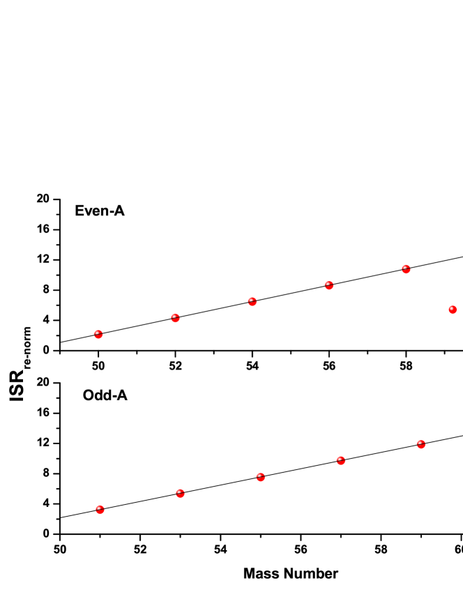
Fig. 1 : Calculated re-normalized Ikeda Sum Rule. The straight line is the theoretical prediction of the sum rule and is shown just to guide the eye.

Fig. 2 : Comparison of calculated B(GT)_- strength distributions in ⁵⁰Cr with measurements and other theoretical model. Exp. 1 shows measured values by (Fujita et al., 2011), Exp. 2 by (Adachi et al., 2007) while KB3G shows shell model calculation by (Petermann et al., 2007). $E_{j}$ represents excitation energy in ⁵⁰Mn in units of MeV.

Fig. 3 : Comparison of calculated B(GT)_- strength distributions in ⁵²Cr with shell model calculation (Petermann et al., 2007). $E_{j}$ represents excitation energy in ⁵²Mn in units of MeV.

Fig. 4 : Comparison of calculated B(GT)_- strength distributions in ⁵⁴Cr with shell model calculation (Petermann et al., 2007). $E_{j}$ represents excitation energy in ⁵⁴Mn in units of MeV.

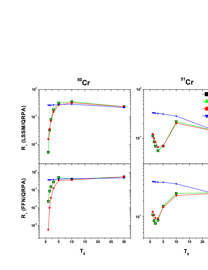
Fig. 5 : The comparison of pn-QRPA neutrino energy loss rates due to ⁵⁰Cr (left) and ⁵¹Cr (right) with the previous calculations performed by LSSM (upper panel) and those performed by FFN (lower panel) as function of stellar temperatures for different selected densities. $\log\rho\text{Y}_{e}$ gives the $\log$ to base 10 of stellar density in units of g cm^-3. T₉ gives the stellar temperature in units of $10^{9}$ K.

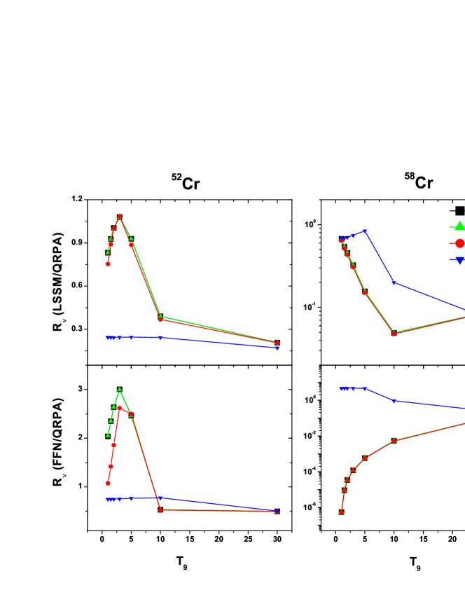
Fig. 6 : Same as Fig. 5 but for neutrino energy loss rates due to ⁵²Cr (left) and ⁵⁸Cr (right)

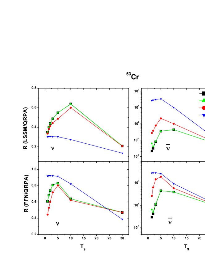
Fig. 7 : The comparison of pn-QRPA neutrino and antineutrino energy loss rates due to ⁵³Cr with the previous calculations performed by LSSM (upper panel) and those performed by FFN (lower panel) as function of stellar temperatures for different selected densities. $\log\rho\text{Y}_{e}$ gives the $\log$ to base 10 of stellar density in units of g cm^-3. T₉ gives the stellar temperature in units of $10^{9}$ K.

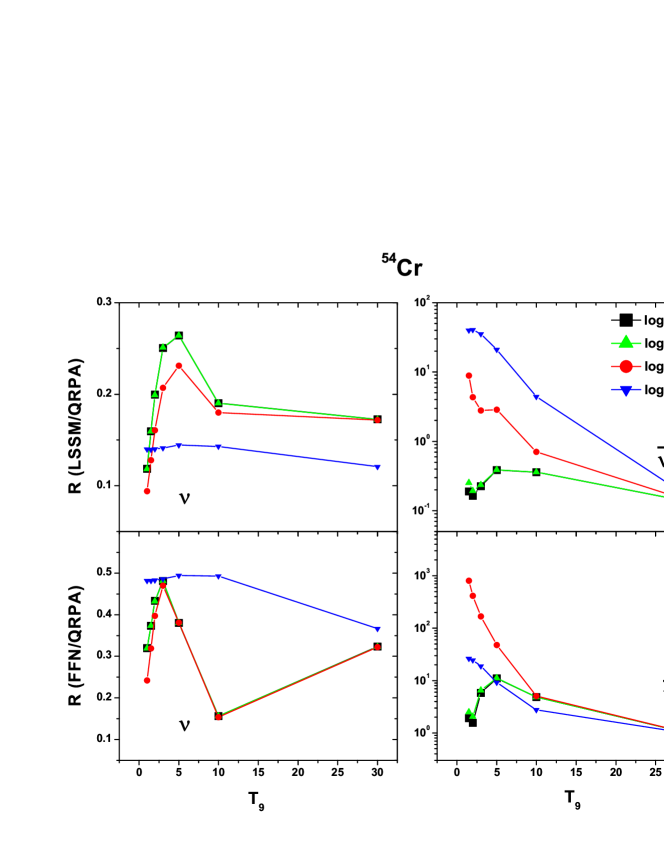
Fig. 8 : Same as Fig. 7 but due to ⁵⁴Cr.

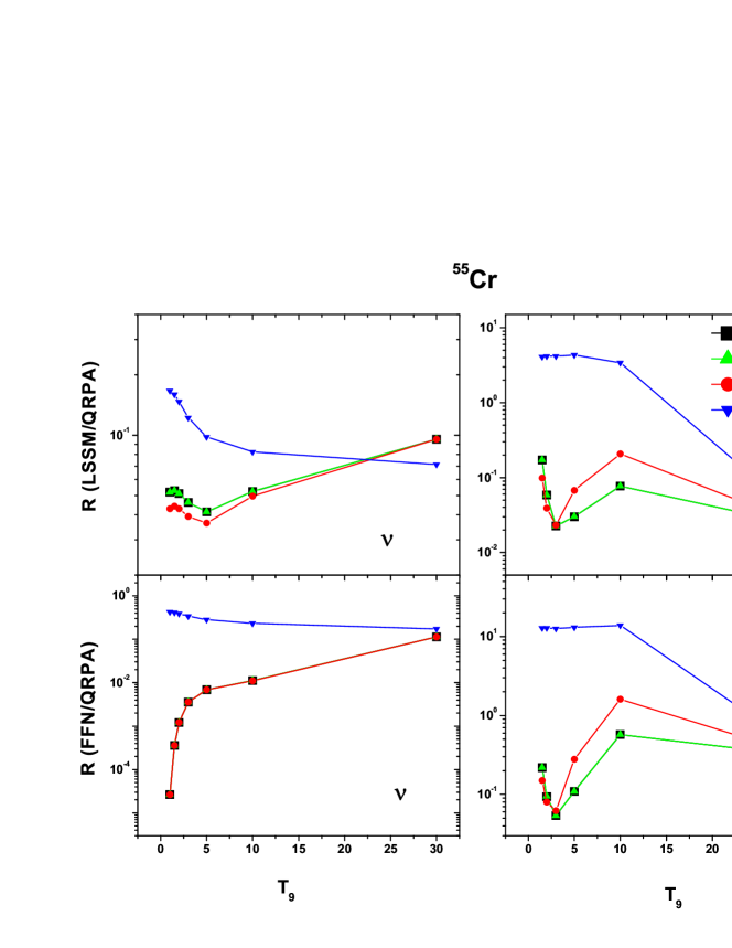
Fig. 9 : Same as Fig. 7 but due to ⁵⁵Cr.

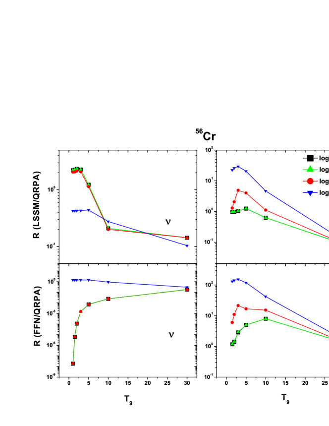
Fig. 10 : Same as Fig. 7 but due to ⁵⁶Cr.

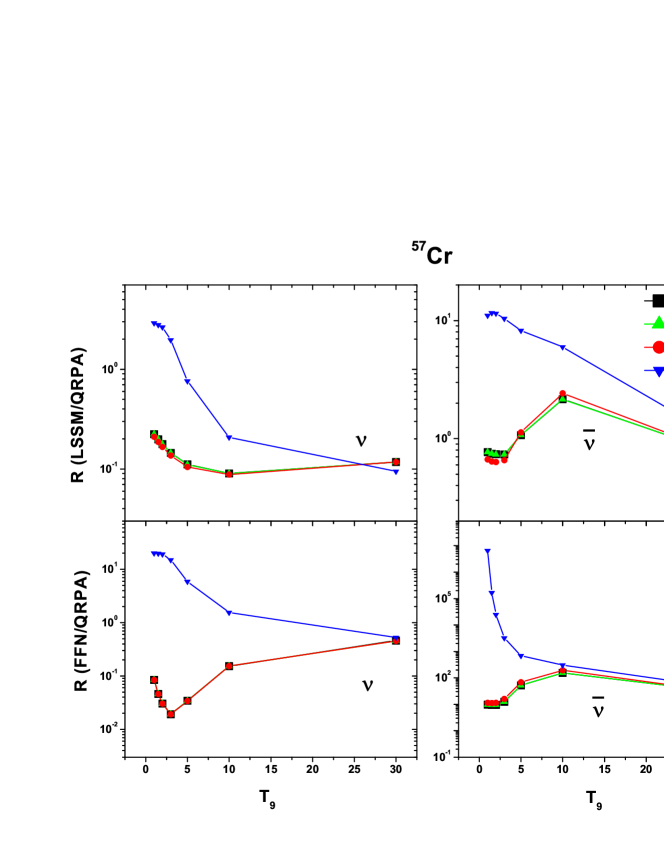
Fig. 11 : Same as Fig. 7 but due to ⁵⁷Cr.

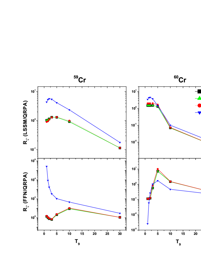
Fig. 12 : Same as Fig. 5 but for antineutrino energy loss rates due to ⁵⁹Cr (left) and ⁶⁰Cr (right)

Table 1 : Total strength, centroid and width of calculated GT strength distributions (for $\beta$-decay and electron capture directions) for ^50-60Cr.

Nuclei	$\sum B(GT)_{-}$	$\sum B(GT)_{+}$	$\bar{E}_{-}$ (MeV)	$\bar{E}_{+}$ (MeV)	Width- (MeV)	Width+ (MeV)
50Cr	4.65	2.49	4.81	4.16	2.12	2.3
51Cr	5.13	1.87	7.72	7.96	3.06	2.41
52Cr	6.55	2.21	5.41	3.27	2.44	1.92
53Cr	5.91	0.51	8.81	6.21	2.79	2.71
54Cr	8.45	1.95	6.19	2.88	2.97	3.32
55Cr	7.94	0.39	9.57	4.06	3.05	3.47
56Cr	9.95	1.31	6.44	1.77	2.59	2.14
57Cr	9.98	0.25	9.62	5.21	2.98	2.84
58Cr	11.6	0.82	6.85	1.57	2.83	2.49
59Cr	12.1	0.24	6.86	1.26	4.79	2.24
60Cr	13.4	0.39	7.74	3.03	3.3	4.99

Table 2 : Comparison of calculated total $B(GT)$ values in ^50,52,53,54Cr with measurement and other theoretical models (LSSM (KB3G) $\rightarrow$ Petermann et al. (2007), SMMC (KB3) $\rightarrow$ Langanke et al. (1995), Shell Model $\rightarrow$ Nakada et al. (1996) and Shell Model (KB3) $\rightarrow$ Caurier et al. (1995)). Experimental data was taken from Adachi et al. (2007).

	50Cr		52Cr		53Cr		54Cr
	$\sum B(GT)_{-}$	$\sum B(GT)_{+}$	$\sum B(GT)_{-}$	$\sum B(GT)_{+}$	$\sum B(GT)_{-}$	$\sum B(GT)_{+}$	$\sum B(GT)_{-}$	$\sum B(GT)_{+}$
pn-QRPA	4.65	2.49	6.55	2.22	5.90	0.51	8.44	1.96
LSSM (KB3G)	5.20	-	8.85	-	-	-	11.13	-
SMMC (KB3)	-	$3.51\pm 0.27$	-	3.51$\pm$0.19	-	-	-	2.21$\pm$0.22
Shell Model	-	-	17.4	4.3	20.1	3.8	22.4	2.9
Shell Model (KB3)	-	3.57	-	-	-	-	-	-
Exp.	2.69	-	-	-	-	-	-	-

Table 3 : Neutrino and antineutrino energy loss rates due to ^50,51,52,53Cr for selected densities and temperatures in stellar matter. $\log\rho\text{Y}_{e}$ has units of g cm^-3, where $\rho$ is the baryon density and Y_e is the ratio of the lepton number to the baryon number. Temperatures (T₉) are given in units of $10^{9}$ K. $\lambda_{\nu}$ ($\lambda_{\bar{\nu}}$) are the total neutrino (antineutrino) energy loss rates as a result of $\beta^{+}$ decay and electron capture ($\beta^{-}$ decay and positron capture) in units of MeV s^-1. All calculated rates are tabulated in logarithmic (to base 10) scale. In the table, -100 means that the rate is smaller than 10^-100 MeV s^-1.

$\log\rho\text{Y}_{e}$	T9	50Cr		51Cr		52Cr		53Cr
		$\lambda_{\nu}$	$\lambda_{\bar{\nu}}$	$\lambda_{\nu}$	$\lambda_{\bar{\nu}}$	$\lambda_{\nu}$	$\lambda_{\bar{\nu}}$	$\lambda_{\nu}$	$\lambda_{\bar{\nu}}$
2.0	0.01	-100	-100	-7.99	-100	-100	-100	-100	-100
2.0	0.10	-64.184	-100	-8.452	-100	-100	-100	-100	-45.112
2.0	0.20	-37.285	-100	-8.556	-93.165	-100	-100	-96.304	-29.973
2.0	0.40	-23.451	-100	-8.449	-48.523	-59.425	-66.075	-52.296	-17.72
2.0	0.70	-17.151	-59.608	-8.191	-28.863	-37.187	-38.789	-33.122	-11.164
2.0	1.00	-13.519	-42.43	-7.124	-21.319	-27.246	-28.289	-24.401	-9.072
2.0	1.50	-10.009	-28.721	-5.757	-15.085	-18.942	-19.798	-17.038	-7.477
2.0	2.00	-8.006	-21.691	-4.882	-11.778	-14.604	-15.261	-13.175	-6.467
2.0	3.00	-5.695	-14.497	-3.733	-8.294	-9.986	-10.45	-9.077	-5.122
2.0	5.00	-3.351	-8.409	-2.379	-5.192	-5.745	-6.105	-5.43	-3.493
2.0	10.00	-0.569	-3.009	-0.506	-1.983	-1.522	-1.92	-1.92	-1.182
2.0	30.00	3.184	2.229	3.322	2.669	2.97	2.678	2.884	2.951
5.0	0.01	-100	-100	-5.667	-100	-100	-100	-100	-100
5.0	0.10	-59.658	-100	-5.669	-100	-100	-100	-100	-47.691
5.0	0.20	-33.723	-100	-5.66	-95.628	-100	-100	-92.741	-30.924
5.0	0.40	-20.261	-100	-5.482	-50.659	-56.235	-69.081	-49.106	-18.709
5.0	0.70	-14.13	-62.629	-5.251	-31.31	-34.167	-41.568	-30.101	-13.248
5.0	1.00	-11.459	-44.489	-5.103	-23.227	-25.187	-30.19	-22.341	-10.809
5.0	1.50	-9.119	-29.611	-4.881	-15.966	-18.052	-20.667	-16.148	-8.312
5.0	2.00	-7.683	-22.014	-4.564	-12.099	-14.281	-15.582	-12.851	-6.771
5.0	3.00	-5.636	-14.556	-3.674	-8.352	-9.926	-10.509	-9.017	-5.173
5.0	5.00	-3.342	-8.418	-2.37	-5.201	-5.735	-6.114	-5.421	-3.5
5.0	10.00	-0.568	-3.009	-0.505	-1.984	-1.521	-1.921	-1.918	-1.182
5.0	30.00	3.184	2.23	3.322	2.67	2.971	2.679	2.884	2.952
8.0	0.01	-2.65	-100	-1.454	-100	-100	-100	-100	-100
8.0	0.10	-2.65	-100	-1.453	-100	-100	-100	-84.178	-100
8.0	0.20	-2.645	-100	-1.444	-100	-59.392	-100	-45.153	-72.452
8.0	0.40	-2.626	-100	-1.348	-71.367	-32.205	-90.891	-25.07	-39.23
8.0	0.70	-2.577	-74.916	-1.201	-42.683	-20.095	-53.541	-16.016	-24.516
8.0	1.00	-2.506	-53.607	-1.112	-30.989	-15.018	-38.342	-12.15	-18.239
8.0	1.50	-2.357	-36.578	-1.005	-21.665	-10.844	-26.353	-8.901	-13.037
8.0	2.00	-2.185	-27.667	-0.908	-16.847	-8.599	-20.229	-7.118	-10.301
8.0	3.00	-1.829	-18.434	-0.732	-11.785	-6.103	-13.86	-5.126	-7.39
8.0	5.00	-1.177	-10.615	-0.45	-7.279	-3.602	-8.167	-3.225	-4.815
8.0	10.00	0.161	-3.76	0.218	-2.73	-0.786	-2.664	-1.169	-1.891
8.0	30.00	3.219	2.195	3.357	2.635	3.006	2.644	2.919	2.917
11.0	0.01	5.913	-100	5.802	-100	5.731	-100	5.582	-100
11.0	0.10	5.913	-100	5.798	-100	5.73	-100	5.578	-100
11.0	0.20	5.914	-100	5.801	-100	5.731	-100	5.577	-100
11.0	0.40	5.912	-100	5.802	-100	5.731	-100	5.575	-100
11.0	0.70	5.913	-100	5.807	-100	5.731	-100	5.571	-100
11.0	1.00	5.913	-100	5.811	-100	5.731	-100	5.57	-100
11.0	1.50	5.913	-100	5.816	-93.812	5.731	-98.131	5.569	-84.642
11.0	2.00	5.914	-81.906	5.82	-70.997	5.732	-74.029	5.569	-64.008
11.0	3.00	5.915	-54.671	5.829	-47.962	5.733	-49.728	5.573	-43.213
11.0	5.00	5.918	-32.505	5.844	-29.135	5.737	-29.868	5.585	-26.383
11.0	10.00	5.942	-15.018	5.912	-13.984	5.77	-13.9	5.66	-13.069
11.0	30.00	6.322	-1.635	6.55	-1.195	6.236	-1.185	6.285	-0.912

Table 4 : Same as Table 3 but for ⁵⁴Cr, ⁵⁵Cr, ⁵⁶Cr and ⁵⁷Cr

$\log\rho\text{Y}_{e}$	T9	54Cr		55Cr		56Cr		57Cr
		$\lambda_{\nu}$	$\lambda_{\bar{\nu}}$	$\lambda_{\nu}$	$\lambda_{\bar{\nu}}$	$\lambda_{\nu}$	$\lambda_{\bar{\nu}}$	$\lambda_{\nu}$	$\lambda_{\bar{\nu}}$
2.0	0.01	-100	-100	-100	-2.482	-100	-2.762	-100	-1.053
2.0	0.10	-100	-100	-100	-2.482	-100	-2.762	-100	-1.053
2.0	0.20	-100	-63.135	-100	-2.482	-100	-2.762	-100	-1.044
2.0	0.40	-96.652	-31.8	-82.692	-2.482	-100	-2.762	-100	-0.999
2.0	0.70	-57.864	-18.076	-49.88	-2.464	-72.849	-2.762	-65.044	-0.951
2.0	1.00	-41.311	-13.29	-35.712	-2.249	-51.937	-2.761	-46.356	-0.927
2.0	1.50	-27.874	-9.768	-24.122	-1.576	-35.096	-2.76	-31.245	-0.907
2.0	2.00	-20.983	-7.9	-18.15	-1.128	-26.487	-2.748	-23.502	-0.892
2.0	3.00	-13.85	-5.797	-11.943	-0.689	-17.593	-2.635	-15.502	-0.84
2.0	5.00	-7.731	-3.534	-6.596	-0.3	-9.921	-1.86	-8.702	-0.648
2.0	10.00	-2.354	-0.743	-1.91	0.695	-3.162	0.04	-2.906	-0.102
2.0	30.00	2.734	3.075	2.909	3.6	2.547	3.225	2.492	2.355
5.0	0.01	-100	-100	-100	-2.501	-100	-2.783	-100	-1.054
5.0	0.10	-100	-100	-100	-2.501	-100	-2.783	-100	-1.054
5.0	0.20	-100	-66.698	-100	-2.5	-100	-2.781	-100	-1.045
5.0	0.40	-93.462	-34.991	-79.502	-2.497	-100	-2.778	-100	-1
5.0	0.70	-54.843	-21.097	-46.859	-2.475	-69.828	-2.775	-62.023	-0.952
5.0	1.00	-39.251	-15.35	-33.652	-2.256	-49.877	-2.772	-44.296	-0.928
5.0	1.50	-26.984	-10.658	-23.232	-1.58	-34.206	-2.77	-30.355	-0.907
5.0	2.00	-20.659	-8.224	-17.827	-1.131	-26.163	-2.761	-23.178	-0.892
5.0	3.00	-13.791	-5.856	-11.883	-0.691	-17.533	-2.652	-15.442	-0.841
5.0	5.00	-7.722	-3.543	-6.586	-0.302	-9.912	-1.867	-8.692	-0.649
5.0	10.00	-2.353	-0.744	-1.909	0.694	-3.161	0.04	-2.905	-0.102
5.0	30.00	2.735	3.076	2.909	3.6	2.547	3.226	2.493	2.355
8.0	0.01	-100	-100	-100	-4.442	-100	-100	-100	-1.381
8.0	0.10	-100	-100	-100	-4.437	-100	-27.97	-100	-1.379
8.0	0.20	-100	-100	-100	-4.432	-100	-17.652	-100	-1.371
8.0	0.40	-69.429	-52.982	-55.462	-4.413	-95.294	-11.906	-81.949	-1.329
8.0	0.70	-40.758	-31.853	-32.769	-4.27	-55.76	-9.009	-47.933	-1.283
8.0	1.00	-29.058	-23.194	-23.455	-3.656	-39.698	-7.64	-34.099	-1.259
8.0	1.50	-19.735	-16.173	-15.98	-2.712	-26.966	-6.383	-23.103	-1.234
8.0	2.00	-14.923	-12.493	-12.088	-2.171	-20.433	-5.638	-17.439	-1.211
8.0	3.00	-9.898	-8.599	-7.986	-1.582	-13.642	-4.68	-11.546	-1.129
8.0	5.00	-5.527	-5.078	-4.386	-1.001	-7.714	-2.797	-6.492	-0.863
8.0	10.00	-1.604	-1.41	-1.157	0.072	-2.409	-0.4	-2.153	-0.28
8.0	30.00	2.77	3.041	2.944	3.566	2.582	3.191	2.528	2.321
11.0	0.01	5.595	-100	5.494	-100	4.854	-100	3.966	-100
11.0	0.10	5.59	-100	5.493	-100	4.858	-100	3.968	-100
11.0	0.20	5.592	-100	5.49	-100	4.856	-100	3.969	-100
11.0	0.40	5.593	-100	5.491	-100	4.854	-100	3.975	-100
11.0	0.70	5.593	-100	5.491	-100	4.854	-100	3.982	-100
11.0	1.00	5.593	-100	5.492	-100	4.854	-100	3.986	-96.729
11.0	1.50	5.594	-86.624	5.503	-73.012	4.855	-76.197	3.991	-65.243
11.0	2.00	5.594	-65.265	5.529	-55.054	4.855	-57.373	4.005	-49.357
11.0	3.00	5.596	-43.68	5.593	-36.948	4.857	-38.347	4.119	-33.277
11.0	5.00	5.601	-26.081	5.684	-22.264	4.866	-22.797	4.529	-20.139
11.0	10.00	5.644	-12.298	5.805	-10.87	5.115	-10.649	5.143	-9.963
11.0	30.00	6.105	-0.786	6.284	-0.258	5.961	-0.632	5.901	-1.489

Table 5 : Same as Table 3 but for ⁵⁸Cr, ⁵⁹Cr and ⁶⁰Cr

$\log\rho\text{Y}_{e}$	T9	58Cr		59Cr		60Cr
		$\lambda_{\nu}$	$\lambda_{\bar{\nu}}$	$\lambda_{\nu}$	$\lambda_{\bar{\nu}}$	$\lambda_{\nu}$	$\lambda_{\bar{\nu}}$
2.0	0.01	-100	-0.826	-100	0.396	-100	0.563
2.0	0.10	-100	-0.826	-100	0.396	-100	0.563
2.0	0.20	-100	-0.826	-100	0.396	-100	0.563
2.0	0.40	-100	-0.826	-100	0.395	-100	0.563
2.0	0.70	-89.901	-0.826	-79.134	0.396	-100	0.563
2.0	1.00	-63.491	-0.826	-56.211	0.423	-74.647	0.563
2.0	1.50	-42.335	-0.826	-37.747	0.515	-49.677	0.563
2.0	2.00	-31.552	-0.825	-28.293	0.6	-36.989	0.563
2.0	3.00	-20.493	-0.815	-18.537	0.713	-24.036	0.564
2.0	5.00	-11.197	-0.526	-10.273	0.837	-13.259	0.662
2.0	10.00	-3.512	1.23	-3.414	1.108	-4.519	2.061
2.0	30.00	2.498	3.846	2.397	3.211	2.256	4.241
5.0	0.01	-100	-0.831	-100	0.395	-100	0.561
5.0	0.10	-100	-0.831	-100	0.395	-100	0.561
5.0	0.20	-100	-0.831	-100	0.395	-100	0.561
5.0	0.40	-100	-0.83	-100	0.395	-100	0.562
5.0	0.70	-86.881	-0.829	-76.113	0.396	-100	0.562
5.0	1.00	-61.431	-0.829	-54.151	0.423	-72.587	0.562
5.0	1.50	-41.445	-0.828	-36.857	0.514	-48.787	0.562
5.0	2.00	-31.229	-0.828	-27.97	0.6	-36.665	0.562
5.0	3.00	-20.433	-0.818	-18.477	0.713	-23.976	0.564
5.0	5.00	-11.187	-0.528	-10.263	0.836	-13.25	0.661
5.0	10.00	-3.51	1.23	-3.413	1.108	-4.517	2.061
5.0	30.00	2.499	3.846	2.398	3.212	2.257	4.241
8.0	0.01	-100	-1.82	-100	0.243	-100	0.203
8.0	0.10	-100	-1.818	-100	0.242	-100	0.202
8.0	0.20	-100	-1.817	-100	0.241	-100	0.202
8.0	0.40	-100	-1.813	-100	0.241	-100	0.203
8.0	0.70	-72.79	-1.803	-62.023	0.243	-88.823	0.204
8.0	1.00	-51.234	-1.788	-43.954	0.274	-62.39	0.207
8.0	1.50	-34.193	-1.753	-29.604	0.375	-41.535	0.212
8.0	2.00	-25.489	-1.709	-22.23	0.468	-30.926	0.22
8.0	3.00	-16.536	-1.604	-14.58	0.591	-20.08	0.24
8.0	5.00	-8.987	-1.003	-8.063	0.728	-11.049	0.404
8.0	10.00	-2.758	1.019	-2.661	0.995	-3.765	1.952
8.0	30.00	2.534	3.812	2.433	3.178	2.292	4.209
11.0	0.01	3.857	-100	4.392	-100	3.364	-100
11.0	0.10	3.858	-100	4.394	-100	3.364	-100
11.0	0.20	3.858	-100	4.397	-100	3.364	-100
11.0	0.40	3.857	-100	4.394	-100	3.363	-100
11.0	0.70	3.857	-100	4.389	-100	3.364	-100
11.0	1.00	3.858	-100	4.377	-83.281	3.364	-90.844
11.0	1.50	3.859	-67.836	4.354	-56.099	3.366	-60.964
11.0	2.00	3.86	-50.968	4.334	-42.39	3.368	-45.839
11.0	3.00	3.864	-33.878	4.305	-28.516	3.373	-30.447
11.0	5.00	3.884	-19.842	4.284	-17.163	3.399	-17.701
11.0	10.00	4.643	-8.732	4.755	-8.254	4.155	-7.29
11.0	30.00	5.907	0.016	5.818	-0.609	5.755	0.539

References

- Cowan et al. (2004) J.J. Cowan, F.-K. Thielemann, Phys. Today Oct. issue, (2004) 47.
- Baade et al. (1934) W. Baade and F. Zwicky, Proc. Nat. Acad. Sci, (1934) 254.
- Hirata et al. (1987) K. Hirata et al., Phys. Rev. Lett. 58 (1987) 1490 .
- Bionta et al. (1987) R. M. Bionta et al., Phys. Rev. Lett. 58 (1987) 1494.
- Bethe et al. (1979) H.A. Bethe, G.E. Brown, J. Applegate, et al., Nucl. Phys. A (1979) 487.
- Bethe (1990) H.A. Bethe, Rev. Mod. Phys. (1990) 801.
- Goldreich et al. (1980) P. Goldreich and S.V. Weber, Astrophys. J. (1980) 991.
- Bethe et al. (1985) H.A. Bethe and J.R. Wilson, Astrophys. J. (1985) 14.
- Herant et al. (1994) M. Herant, W. Benz, W.R. Hix, et al., Astrophys. J. (1994) 339.
- Freher et al. (2000) C.L. Freyer and A. Heger, Astrophys. J. (2000) 1033.
- Buras et al. (2003) R. Buras, M. Rampp, H.-T. Janka, et al., Phys. Rev. Lett. (2003) 241101.
- Janka et al. (2003) H.-T. Janka, R. Buras and M. Rampp, Nucl. Phys. A (2003) 269.
- Mezzacappa et al. (2001) A. Mezzacappa, M. Liebendoerfer, O.E. Messer, et al., Phys. Rev. Lett. (2001) 1935.
- Thompson et al. (2003) T.A. Thompson, A. Burrows, and P.A. Pinto, Astrophys. J. (2003) 434.
- Balantekin et al. (2003) A.B. Balantekin and G.M. Fuller, J. Phys. G (2003) 2513.
- Strother et al. (2009) T. Strother and W. Bauer, Prog. Part. Nucl. Phys. (2009) 468.
- Fuller et al. (1980, 1982) G.M. Fuller, W.A. Fowler, and M.J. Newman, Astrophys. J. Suppl. Ser. (1980) 447; (1982)279; Astrophys. J. (1982) 715; (1985) 1.
- Ikeda et al. (1963) K.I. Ikeda, S. Fuji, J.I. Fujita, Phys. Lett. (1963) 27.
- Zioni et al. (1972) J. Zioni, A.A. Jaffe, E. FriedMan, N. Haik, , R. Schectman and D. Nir, Nucl. Phys. A , (1972) 465.
- Onishi et al. (2005) T.K. Onishi, A. Gelberg, H. Sakurai, K. Yoneda, N. Aoi, N. Imai, H. Baba, P. von Brentano, N. Fukuda, Y. Ichikawa, M. Ishihara, H. Iwasaki, D. Kameda, T. Kishida, A.F. Lisetskiy, H.J. Ong, M. Osada, T. Otsuka, M.K. Suzuki, K. Ue, Y. Utsuno and H. Watanabe, Phys. Rev. C , (2005) 024308 .
- Fujita et al. (2011) Y. Fujita, B. Rubio, W. Gelletly, Prog. Part. Nucl. Phys. , (2011) 549.
- Adachi et al. (2007) T. Adachi et al. Nucl. Phys. A , (2007) 70c .
- Aufderheide et al. (1994) M.B. Aufderheide, I. Fushiki, S. E. Woosley, et al., Astrophys. J. Suppl. (1994) 389.
- Nabi et al. (1999) J.-U. Nabi and H.V. Klapdor-Kleingrothaus, Eur. Phys. J. A (1999) 337.
- Langanke et al. (2000) K. Langanke and G. Martínez-Pinedo, Nucl. Phys. A 673 (2000) 481.
- Heger et al. (2001) A. Heger, S. E. Woosley, G. Martínez-Pinedo, K. Langanke, Astrophys. J. 560 (2001) 307.
- Nabi et al. (2004) J.-U. Nabi and H.V. Klapdor-Kleingrothaus, At. Data Nucl. Data Tables (2004) 237.
- Petermann et al. (2007) I. Petermann, G. Martínez-Pinedo, K. Langanke, and E. Caurier, Eur. Phys. J. A , (2007) 319.
- Langanke et al. (1995) K. Langanke, D.J. Dean, P.B. Radha, Y. Alhassaid, and S.E. Koonin, Phys. Rev. C , (1995) 718.
- Caurier et al. (1995) E. Caurier, G. Martínez-Pinedo, A. Poves, A.P. Zuker, Phys. Rev. C , (1995) R1736.
- Nakada et al. (1996) H. Nakada, and T. Sebe J. Phys. G: Nucl. Part. Phys. , (1996) 1349.
- Nabi et al. (1999) J.-U. Nabi and H.V. Klapdor-Kleingrothaus, At. Data Nucl. Data Tables (1999) 149.
- Nabi et al. (2005) J.-U. Nabi and M.-U. Rahman, Phys. Lett. B (2005) 190.
- Nabi et al. (2007) J.-U. Nabi and M.-U. Rahman, Phys. Rev. C (2007) 035803.
- Nabi et al. (2007) J.-U. Nabi and M. Sajjad, Phys. Rev. C (2007) 055803.
- Nabi et al. (2007) J.-U. Nabi, M. Sajjad, and M.-U. Rahman, Acta Phys. Pol. B (2007) 3203.
- Staudt et al. (1990) A. Staudt, E. Bender, K. Muto and H.V. Klapdor-Kleingrothaus, At. Data Nucl. Data Tables , (1990) 79.
- Hirsch et al. (1993) M. Hirsch, A. Staudt, K. Muto and H.V. Klapdor-Kleingrothaus, At. Data Nucl. Data Tables , (1993) 165.
- Raman et al. (1987) S. Raman, C.H. Malarkey, W.T. Milner, C.W. Nestor, P.H.Jr. Stelson, At. Data Nucl. Data Tables, , (1987) 1.
- Möller et al. (1981) P. Möller, and J.R. Nix, At. Data Nucl. Data Tables , (1981) 165.
- Audi et al. (2012) G. Audi, M. Wang, A.H. Wapstra, F.G. Kondev, M. MacCormick, X. Xu and B. Pfeiffer, Chin. Phys. C, 36 (2012) 1287 ; M. Wang, G. Audi, A.H. Wapstra, F.G. Kondev, M. MacCormick, X. Xu and B. Pfeiffer B, Chin. Phys. C, 36 (2012) 1603.
- Aufderheide et al. (1996) M.B. Aufderheide, S.D. Bloom, G.J. Mathews, and D.A. Resler, Phys. Rev. C , (1996) 3139.
- Vetterli et al. (1989) M.C. Vetterli, O. Häusser, R. Abegg, W.P. Alford, A. Celler, D. Frekers, R.Helmer, R. Henderson, K.H. Hicks, K.P. Jackson, R.G. Jeppesen, C.A. Miller, K. Raywood, and S. Yen, Phy. Rev. C , (1989) 559.
- Gaarde (1983) C. Gaarde, Nucl. Phys. A 396 (1983) 127c.
- Rönnqvist et al. (1993) T. Rönnqvist, H. Condé, N. Olsson, E. Ramström, R. Zorro, J. Blomgren, A. Håkansson, A. Ringbom, G. Tibell, O. Jonsson, L. Nilsson, P.-U. Renberg, S. Y. van der Werf, W. Unkelbach, and F. P. Brady, Nucl. Phys. A 563 (1993) 225.
- Rodin et al. (2006) V. Rodin, A. Faessler, F. Simkovic, and P. Vogel, Czech. J. Phys. 56 (2006) 495.
- Yost et al. (1988) G. P. Yost et al. (Particle Data Group), Phys. Lett. B204 (1988) 1.
- Gove and Martin (1971) N. B. Gove and M. J. Martin, At. Data Nucl. Data Tables, 10 (1971) 205.
- Nilsson (1955) S. G. Nilsson, Mat. Fys. Medd. Dan. Vid. Selsk 29, 16 (1955).
- Hirsch et al. (1991) M. Hirsch, A. Staudt, K. Muto, and H. V. Klapdor-Kliengrothaus, Nucl. Phys. A535, 62 (1991).
- Cakmak et al. (2015) S. Cakmak, J.-U. Nabi, T. Babacan and I. Maras, Adv. Space Res. (2015) 440.
- Langanke et al. (1998) K. Langanke and G. Martínez-Pinedo, Phys. Lett. B436 (1998) 19.
- Pruet et al. (2003) J. Pruet and G. M. Fuller, Astrophys. J. Suppl. Ser. 149 (2003) 189-203.