Evaluation of Generalized Degrees of Freedom for Sparse Estimation by Replica Method

Abstract

We develop a method to evaluate the generalized degrees of freedom (GDF) for linear regression with sparse regularization. The GDF is a key factor in model selection, and thus its evaluation is useful in many modelling applications. An analytical expression for the GDF is derived using the replica method in the large-system-size limit with random Gaussian predictors. The resulting formula has a universal form that is independent of the type of regularization, providing us with a simple interpretation. Within the framework of replica symmetric (RS) analysis, GDF has a physical meaning as the effective fraction of non-zero components. The validity of our method in the RS phase is supported by the consistency of our results with previous mathematical results. The analytical results in the RS phase are calculated numerically using the belief propagation algorithm.

Keywords: Cavity and replica method, Statistical inference, Learning theory

1 Introduction

Statistical modelling plays a key role in extracting the structures of a system that may be hidden behind observed data and using them for prediction or control. A statistical model approximates the true generative process of the data, which is generally expressed by a probability distribution. Although it is necessary to adopt an appropriate statistical model, this will depend on the purpose of the modelling, and the definition of appropriateness is not unique. Akaike proposed an information criterion for model selection, where the appropriate model is defined using Kullback–Leibler divergence [1]. This criterion validates the relative effectiveness of the model under consideration, and mathematically expresses the contribution of the model to the prediction performance.

Since the systemization of the least absolute shrinkage and selection operator (LASSO) [2], which simultaneously achieves variable selection and estimation, sparse estimation has been attracting considerable attention in fields such as signal processing [3, 4] and machine learning [5, 6]. In general, sparse estimation is formulated as the problem of minimizing the estimating function penalized by sparse regularization. The estimated variables have zero components, a property known as sparsity. To find the sparse representation of the system from among various candidates, a seemingly hidden rule that controls the system is sought. Similar to LASSO, $\ell_{1}$ regularization is widely used because of its convexity, which yields mathematical and algorithmic tractability [3]. In addition, non-convex regularization, such as using the $\ell_{p}~{}(p<1)$-norm [7, 8], has been studied to obtain a sparser representation than that given by $\ell_{1}$-norm regularization [9]. Furthermore, the smoothly clipped absolute deviation (SCAD) and adaptive LASSO penalty have been investigated [10, 11, 12] to acquire the oracle property, which the LASSO estimator does not possess.

The emergence of the estimation paradigm associated with sparsity requires the development of appropriate model selection criteria. In sparse estimation, the determination of the regularization parameter can be regarded as the selection of a model from a family of models that have different sparsities controlled by the regularization parameter. In addition to the cross-validation (CV) method [13], which is a simple numerical approach for sparse estimation [14, 15], analytical model selection methods with lower computational costs have been developed. One such method involves estimating the generalized degrees of freedom (GDF) [16]. The GDF is a key quantity for Mallows’ $C_{p}$, a model selection criterion based on the prediction error [17]. In particular, the derivation of GDF has been studied in linear regression with a known variance [18]. The analytical form of the GDF for LASSO [19] and elastic net regularization [20] are well known, but general expressions for other regularizations have not yet been derived.

In this paper, we propose an analytical method based on statistical physics for the derivation of GDF in sparse estimation. Certain aspects of statistical physics developed for random systems have already been applied to sparse estimation problems [21, 22, 23, 24]. The analysis of typical properties provides physical interpretations of the problems based on phase transition pictures, and this contributes to the development of algorithms [25, 26, 27, 28]. The statistical physical method can be applied to the estimation of GDF for sparse regularization. We show that GDF is expressed as the effective fraction of non-zero components for any sparse regularization. This expression is a mathematical realization of the meaning of GDF in terms of “model complexity” [19, 29].

The remainder of this paper is organized as follows. Section 2 summarizes the model selection criterion discussed in this paper and highlights some previous related studies on sparse estimation. Section 3 explains our problem setting for the estimation of GDF. Sections 4 and 5 describe our analytical method based on the replica method for sparse estimation. Section 6 represents the behaviour of GDF for $\ell_{1}$, elastic net, $\ell_{0}$, and SCAD regularization. Section 7 proposes the numerical calculation of GDF using the belief propagation algorithm, and discusses the generality of the results. In Section 8, the approximation performance of our method for the calculation of GDF is examined in the case of $\ell_{0}$ regularization. Finally, Section 9 concludes the paper.

2 Overview of model selection

In this section, we explain the criteria for model selection discussed in this paper. In addition, we summarize previous studies and identify our contributions. We focus on the parametric model, where the true generative model of $z$, denoted by $q(z)$, is approximated by $p(z|\bm{\theta})$ with a parameter $\bm{\theta}\in\bm{\Theta}\subset\mathbb{R}^{N}$, where $\bm{\Theta}$ is a parameter space. The parameter is estimated under the given model to effectively describe the true distribution using training data $\bm{w}=\{w_{\mu}\}$ $(\mu=1,\cdots,M,w_{\mu}\sim q(w_{\mu}))$. Let us prepare a set of candidate models ${\cal M}=\{p_{1}(z|\hat{\bm{\theta}}_{1}),\cdots,p_{m}(z|\hat{\bm{\theta}}_{m})\}$ for the approximation of the true distribution, where $\hat{\bm{\theta}}_{k}$ is the estimated parameter under the $k$-th model. Model selection is then the problem of adopting a model based on a certain criterion.

2.1 Information criterion

The information criterion evaluates the quality of the statistical model based on Kullback–Leibler (KL) divergence. KL divergence describes the closeness between the true distribution $q(z)$ and the assumed distribution $p(z|\hat{\bm{\theta}}_{\rm ML}(\bm{w}))$ as

$${\rm KL}(q:p)=E_{z\sim q(z)}\left[\log{q(z)}\right]-E_{z\sim q(z)}[\log{p(z|\hat{\bm{\theta}}_{\rm ML}(\bm{w}))}],$$ (1)

where $\hat{\bm{\theta}}_{\rm ML}(\bm{w})$ is the maximum likelihood estimator from the training sample $\bm{w}$. The dependency on the model appears only in the second term of (1), called the predicting log-likelihood, i.e. $l(\bm{w})\equiv E_{z\sim q(z)}[\log{p(z|\hat{\bm{\theta}}_{\rm ML}(\bm{w}))}]$. Therefore, the maximization of the predicting log-likelihood is the basis for the information criterion. Unfortunately, it is generally impossible to evaluate the predicting log-likelihood, because we cannot determine the true distribution. We define the estimator of the predicting log-likelihood using the empirical distribution

$$\hat{l}(\bm{w})=\frac{1}{M}\sum_{\mu=1}^{M}\log p(w_{\mu}|\hat{\bm{\theta}}_{\rm ML}(\bm{w})),$$ (2)

which corresponds to the maximum log-likelihood. The expected value of the difference between the predicting log-likelihood and the maximum log-likelihood, termed the bias, is given by

$$b=E_{\bm{w}\sim q(\bm{w})}\left[\hat{l}(\bm{w})-E_{z\sim q(z)}\left[\log p(z|\hat{\bm{\theta}}_{\rm ML}(\bm{w}))\right]\right],$$ (3)

where $q(\bm{w})=\prod_{\mu}q(w_{\mu})$. The information criterion is defined as an unbiased estimator of the negative predicting log-likelihood:

$${\rm IC}(\bm{w})=-2\hat{l}(\bm{w})+2\hat{b}(\bm{w}),$$ (4)

where $\hat{b}(\bm{w})$ is an unbiased estimator of the bias, and the coefficient $2$ is a conventional value. The optimal model is defined as that which minimizes ${\rm IC}(\bm{w})$ among the models in ${\cal M}$. Intuitively, the first and second terms represent the training error and the complexity of the model, respectively. As the complexity of the model increases, the model can express various distributions. However, overfitting is likely to occur, which hampers the prediction of unknown data. The information criterion selects the model that achieves the best trade-off between the training error and the level of model complexity.

The values of $b$ can be calculated asymptotically. In particular, when the statistical model contains the true model, namely a parameter $\bm{\theta}^{*}$ exists such that $q(z)=p(z|\bm{\theta}^{*})$, the information criterion is known as Akaike’s information criterion (AIC), where the bias term $b$ is reduced to the dimension of the parameter $\bm{\theta}$ [1].

The criterion explained thus far is for models constructed by maximum likelihood estimation. To determine the parameter with other learning strategies, we focus on maximum likelihood estimation under regularization, where the GDF facilitates the extension of the information criterion [29]. A general expression of GDF is naturally derived from another model selection criterion, namely, Mallows’ $C_{p}$ [17].

2.2 Mallows’ $C_{p}$ and generalized degrees of freedom

The prediction of unknown data is another criterion for the evaluation of a model. We define the squared prediction error per component as

$${\rm err}_{\rm pre}(\bm{w})=\frac{1}{M}E_{\bm{z}}[||\bm{z}-\hat{\bm{w}}(\bm{w})||_{2}^{2}],$$ (5)

where $\hat{\bm{w}}$ is the estimate of $\bm{w}$ and $\bm{z}\in\mathbb{R}^{M}$ is independent of $\bm{w}\in\mathbb{R}^{M}$, but each component of $\bm{z}$ is generated according to the same distribution as $\bm{w}$. When the training sample is generated as $\bm{w}\sim{\cal N}(\bm{\mu},\sigma^{2}\bm{I}_{M})$, where $\bm{I}_{M}$ is the $M$-dimensional identity matrix, Mallows’ $C_{p}$, calculated as

$${c_{p}}(\bm{w})={\rm err}_{\rm train}(\bm{w})+2\sigma^{2}\hat{\rm df}(\bm{w}),$$ (6)

is an unbiased estimator of the prediction error. Here,

$${\rm err}_{\rm train}(\bm{w}) =\frac{1}{M}||\bm{w}-\hat{\bm{w}}(\bm{w})||_{2}^{2}$$ (7)

is the training error and $\hat{\rm df}(\bm{w})$ is an unbiased estimator of GDF defined by

$${\rm df}=\frac{{\rm cov}(\bm{w},\hat{\bm{w}}(\bm{w}))}{M\sigma^{2}},$$ (8)

which quantifies the complexity of the model [19, 29], where ${\rm cov}(\bm{w},\hat{\bm{w}}(\bm{w}))=E_{\bm{w}}[(\bm{w}-E_{\bm{w}}[\bm{w}])(\hat{\bm{w}}(\bm{w})-E_{\bm{w}}[\hat{\bm{w}}(\bm{w})])]$. In the framework of $C_{p}$, the optimal model is defined as that which minimizes $c_{p}(\bm{w})$ among the models in ${\cal M}$.

Another expression of GDF is given by [16]

$${\rm df}=\frac{1}{M}\sum_{\mu}E_{\bm{\bm{w}}}\left[\frac{\partial\hat{w}_{\mu}(\bm{w})}{\partial w_{\mu}}\right],$$ (9)

which corresponds to the expectation of Stein’s unbiased risk estimate (SURE) for the prediction error [30]. GDF was originally introduced as an extension of the degrees of freedom in the linear estimation rule for a general modelling procedure in the form (9) [16].

When the assumed model obeys a Gaussian distribution $p(\bm{w}|\bm{\theta})\propto\exp(-\frac{1}{2\sigma^{2}}||\bm{w}-\bm{\mu}(\bm{\theta})||_{2}^{2})$ with a known variance, and taking $\bm{\mu}(\hat{\bm{\theta}}_{\rm ML}(\bm{w}))=\hat{\bm{w}}(\bm{w})$, AIC (normalized by the number of training samples) is given by [19]

$${\rm AIC}(\bm{w})=\frac{{\rm err}_{\rm train}(\bm{w})}{\sigma^{2}}+2\hat{\rm df}(\bm{w}).$$ (10)

Equations (6) and (10) indicate that model selection based on AIC and that based on $C_{p}$ give the same result; they are proportional to each other $c_{p}(\bm{w})=\sigma^{2}{\rm AIC}(\bm{w})$.

2.3 Model selection for sparse regularization and our contributions

The regression problems with sparse regularization is formulad as

$$\min_{\bm{x}}\left\{e(\bm{x};\bm{w},\bm{A})+r(\bm{x};\eta)\right\},$$ (11)

where $e(\bm{x};\bm{w},\bm{A})$ measures the difference between training data $\bm{w}$ and its fit using regression coefficients $\bm{x}$ under the predictor matrix $\bm{A}$, and $r(\bm{x};\eta)$ is the regularization term with the regularization parameter $\eta$ that enhances zero components in $\bm{x}$. The regularization parameter determines the number of predictors used in the expression of the data distribution, and the model distribution under the determined number of predictors can be regarded as a model: ${\cal M}=\{p_{\eta}(z|\hat{\bm{\theta}}_{\eta})|\eta\in\bm{H}\}$, where $\bm{H}$ is the support of the regularization parameter. Therefore, tuning the regularization parameter $\eta$ corresponds to model selection. However, in general, the derivation of AIC based on the asymptotic expansion is not straightforwardly applicable to sparse regularization. In such cases, $C_{p}$ is useful for deriving the model selection criterion when the squared error is considered. In LASSO, it is mathematically proven that, when the number of training samples is greater than the number of predictors, the ratio of the number of non-zero regression coefficients to the number of training samples is an unbiased estimator of the degrees of freedom in a finite sample [19]. However, the derivation of GDF is analytically difficult for general sparse regularizations. To overcome this difficulty, GDF computation techniques have been developed using the parametric bootstrap method [18] and SURE [30, 31].

In the present paper, we propose an estimation technique for GDF using the replica method under a replica symmetric (RS) assumption for linear regression with Gaussian i.i.d. predictors. The replica symmetric analysis for the estimation problems under sparse regularization are shown in [21, 22, 23, 24]. In these papers, the replica method is employed to study phase transition or the property of estimators. We extend this analytical method for the calculation of GDF that is not taken into account in the current formalism of the replica analysis. The technique we propose is applicable to general sparse regularization. Using our method, the correspondence between GDF and the effective fraction of non-zero components in the large-system-size limit is shown to be independent of the form of regularization. Our approach differs from previous methods in which GDF has been derived for specific types of regularization. We apply our method to $\ell_{1}$, elastic net, $\ell_{0}$, and SCAD regularization to obtain the GDF. The results shown here for $\ell_{1}$ and elastic net regularization are weaker than those in previous studies, where the unbiased estimator of GDF, $\hat{\rm df}$, is derived for one instance of the predictor. However, our method is consistent with previous results, which supports the validity of our approach. Furthermore, our method can be applied to non-convex sparse regularizations such as $\ell_{0}$ and SCAD, and extends the discussion of GDF to general sparse regularization. For the $\ell_{0}$ case, the solution under the RS assumption is always unstable against perturbations that break the replica symmetry, but we show that GDF under the RS assumption approximates the true value of GDF. In the case of SCAD regularization, our method can identify the most appropriate model based on the prediction error within the range of the RS assumption when the mean of the data is sufficiently small. The generality of the result in terms of the correspondence between GDF and the effective fraction of non-zero components is discussed using a belief propagation algorithm for other predictor matrices.

3 Problem setting and formulation

We apply a linear regression model with sparse regularization $r(\bm{x};\eta)=\sum_{i}r(x_{i};\eta)$, where $\eta$ is a regularization parameter, to a set of training data $\bm{y}\in\mathbb{R}^{M}$:

$$\min_{\bm{x}}\left\{\frac{1}{2}||\bm{y}-\bm{Ax}||_{2}^{2}+r(\bm{x};\eta)\right\},$$ (12)

where the column vectors of $\bm{A}=\{\bm{A}_{1},\cdots,\bm{A}_{N}\}\in\mathbb{R}^{M\times N}$ and components of $\bm{x}\in\mathbb{R}^{N}$ correspond to predictors and regression coefficients, respectively. Here, the coefficient of the squared error, $1/2$, is introduced for mathematical convenience. The variable $\bm{x}$ to be estimated here corresponds to the parameter $\bm{\theta}$ in the previous section, and the number of non-zero components in $\bm{x}$ corresponds to the number of parameters used in the model. We introduce the posterior distribution of $\bm{x}$:

$$P_{\beta}(\bm{x}|\bm{y},\bm{A})=\exp\left\{-\frac{\beta}{2}||\bm{y}-\bm{Ax}||_{2}^{2}-\beta r(\bm{x};\eta)-\ln Z_{\beta}(\bm{y},\bm{A})\right\},$$ (13)

where $Z_{\beta}(\bm{y},\bm{A})$ is the normalization constant. The distribution as $\beta\to\infty$ is the uniform distribution over the minimizers of (12). Estimate of the solution of (12) under a fixed set of $\{\bm{y},\bm{A}\}$, denoted by $\hat{\bm{x}}(\bm{y},\bm{A})$, is given by

$$\hat{\bm{x}}(\bm{y},\bm{A})=\lim_{\beta\to\infty}\langle\bm{x}\rangle_{\beta},$$ (14)

where $\langle\cdot\rangle_{\beta}$ denotes the expectation according to (13) at $\beta$. Using this estimate $\hat{\bm{x}}(\bm{y},\bm{A})$ of $\bm{x}$, the training sample $\bm{y}$ is estimated as

$$\hat{\bm{y}}(\bm{y},\bm{A})=\bm{A}\hat{\bm{x}}(\bm{y},\bm{A}).$$ (15)

To understand the typical performance of (12), we calculate the expectation of the training error with respect to $\bm{y}$ and $\bm{A}$,

$$\overline{\rm err}_{\rm train}=E_{\bm{y},\bm{A}}[{\rm err}_{\rm train}(\bm{y},\bm{A})].$$ (16)

At a sufficiently large system size $N\to\infty$, we set the scaling relationship as $\alpha=M/N\sim O(1)$ and $\hat{\rho}=K/N\sim O(1)$, where $K$ is the number of non-zero components of $\hat{\bm{x}}$. The training error relates to the free energy density $f$ as [34]

$$f \equiv-\lim_{\beta\to\infty}\frac{1}{N}\frac{\partial}{\partial\beta}\phi_{\beta}=\frac{\alpha\overline{\rm err}_{\rm train}}{2}+\overline{r},$$ (17)

where $\phi_{\beta}\equiv E_{\bm{y},\bm{A}}[\ln Z_{\beta}(\bm{y},\bm{A})]$ and

$$\overline{r}=\frac{1}{N}E_{\bm{y},\bm{A}}[r(\hat{\bm{x}}(\bm{y},\bm{A});\eta)].$$ (18)

The expectation of the regularization term $\overline{r}$ is derived separately from $f$, as shown in the following section. Hence, the training error is derived as

$$\overline{\rm err}_{\rm train} =\frac{2(f-\overline{r})}{\alpha}.$$ (19)

For the calculation of GDF, we introduce external fields $\kappa$ and $\nu$, and define the extended posterior distribution as

$$P_{\beta,\kappa,\nu}(\bm{x}|\bm{y},\bm{A}) \!=\!\exp\left\{-\frac{\beta}{2}||\bm{y}\!-\!\bm{Ax}||_{2}^{2}\!-\!\beta r(\bm{x};\eta)\!-\!\beta\!\sum_{\mu i}(\kappa y_{\mu}\!+\!\nu)A_{\mu i}x_{i}\!-\!\ln Z_{\beta,\kappa,\nu}(\bm{y},\!\bm{A})\right\},$$

(20)

where $Z_{\beta,\kappa,\nu}(\bm{y},\bm{A})$ is the normalization constant. We define the extended free energy density as

$$f_{\kappa,\nu} =-\lim_{\beta\to\infty}\frac{1}{N}\frac{\partial}{\partial\beta}\phi_{\beta,\kappa,\nu},$$ (21)

where $\phi_{\beta,\kappa,\nu}=E_{\bm{y},\bm{A}}[\ln Z_{\beta,\kappa,\nu}(\bm{A},\bm{y})]$ and $f=f_{\kappa=0,\nu=0}$. We derive the following quantities from the extended free energy density:

$$\hat{\gamma} \equiv\frac{1}{M}\sum_{\mu}E_{\bm{y},\bm{A}}[y_{\mu}\sum_{i}A_{\mu i}\hat{x}_{i}(\bm{y},\bm{A})]=\frac{1}{\alpha}\frac{\partial}{\partial\kappa}f_{\kappa,\nu}\Big{|}_{\kappa,\nu=0}$$ (22)

$$\hat{m}_{y} \equiv\frac{1}{M}\sum_{\mu}E_{\bm{y},\bm{A}}[\sum_{i}A_{\mu i}\hat{x}_{i}(\bm{y},\bm{A})]=\frac{1}{\alpha}\frac{\partial}{\partial\nu}f_{\kappa,\nu}\Big{|}_{\kappa,\nu=0}.$$ (23)

Using these, the GDF for a Gaussian training sample is derived as

$${\rm df}=\frac{\hat{\gamma}-\hat{m}_{y}m_{y}}{\sigma_{y}^{2}},$$ (24)

where $m_{y}\in\mathbb{R}$ and $\sigma_{y}^{2}\in\mathbb{R}$ are the mean and variance of the training sample, respectively. Further, $C_{p}$ given by (6) is the unbiased estimator of the prediction error. Hence, the expectation of the prediction error with respect to $\bm{y}$ and $\bm{A}$,

$$\overline{\rm err}_{\rm pre}=\frac{1}{M}E_{\bm{y},\bm{A}}[E_{\bm{z}}[||\bm{z}-\hat{\bm{y}}(\bm{y},\bm{A})||_{2}^{2}]],$$ (25)

is given by

$$\overline{\rm err}_{\rm pre}=\overline{\rm err}_{\rm train}+2\sigma_{y}^{2}{\rm df}.$$ (26)

4 Analysis

For the derivation of GDF, we resort to the replica method [32, 33]. The RS calculations for $\ell_{0}$ and $\ell_{1}$ minimization are shown in the typical performance analysis of compressed sensing [21] and dictionary learning [24]. We summarize the analytical method and explain how it can be extended to the evaluation of GDF. Hereafter, we consider Gaussian i.i.d. predictors $A_{\mu i}\sim{\cal N}(0,M^{-1})~{}\forall(\mu,i)$.

4.1 Replica method and replica symmetry

We calculate the generating function $\phi_{\beta}$ using the following identity:

$$E_{\bm{y},\bm{A}}[\ln Z_{\beta}(\bm{y},\bm{A})]=\lim_{n\to 0}\frac{E_{\bm{y},\bm{A}}[Z_{\beta}^{n}(\bm{y},\bm{A})]-1}{n}.$$ (27)

Assuming that $n$ is a positive integer, we can express the expectation of $Z_{\beta}^{n}(\bm{y},\bm{A})$ by introducing $n$ replicated systems:

$$E_{\bm{y},\bm{A}}[Z_{\beta}^{n}(\bm{y},\bm{A})] =\int d\bm{A}d\bm{y}P_{A}(\bm{A})P_{y}(\bm{y})\int d\bm{x}^{(1)}\cdots d\bm{x}^{(n)}$$ (28)

$$\times\exp\Big{[}\sum_{a=1}^{n}\Big{\{}-\frac{\beta}{2}||\bm{y}-\bm{Ax}^{(a)}||_{2}^{2}-\beta r(\bm{x}^{(a)};\eta)\Big{\}}\Big{]},$$

where $P_{A}(\bm{A})=\prod_{\mu,i}\sqrt{\frac{M}{2\pi}}\exp(-\frac{M}{2}A_{\mu i}^{2})$ and $P_{y}(\bm{y})=\prod_{\mu}\sqrt{\frac{1}{2\pi\sigma_{y}^{2}}}\exp(-\frac{1}{2\sigma_{y}^{2}}(y-m_{y})^{2})$. We characterize the microscopic states of $\{\bm{x}^{(a)}\}$ with the macroscopic quantities

$$q^{(ab)} =\frac{1}{M}\sum_{i}x_{i}^{(a)}x_{i}^{(b)}.$$ (29)

Introducing the identity for all combinations of $a,b~{}(a\leq b)$

$$1=\int dq^{(ab)}\delta\left(q^{(ab)}-\frac{1}{M}\sum_{i}x_{i}^{(a)}x_{i}^{(b)}\right),$$ (30)

the integration with respect to $\bm{A}$ leads to the following expression:

$$E_{\bm{y},\bm{A}}[Z_{\beta}^{n}(\bm{y},\bm{A})] =\int d{\cal Q}{\cal S}({\cal Q})\int\{d\bm{u}^{(a)}\}P_{u}(\{\bm{u}^{(a)}\}|{\cal Q})\int d\bm{y}P_{y}(\bm{y})$$ (31)

$$\times\exp\Big{\{}-\frac{\beta}{2}\sum_{a}||\bm{y}-\bm{u}^{(a)}||^{2}_{2}\Big{\}},$$

where each component of $\bm{u}^{(a)}$, denoted by $u_{\mu}^{(a)}$, is statistically equivalent to $\sum_{i}A_{\mu i}x_{i}^{(a)}$, and ${\cal Q}$ is a matrix representation of $\{q^{(ab)}\}$. Setting $\tilde{\bm{u}}_{\mu}=\{u_{\mu}^{(1)},\cdots,u_{\mu}^{(n)}\}$, its probability distribution is given by [21]

$$P_{u}(\{\bm{u}^{a}\}|{\cal Q})=\prod_{\mu}\frac{1}{\sqrt{(2\pi)^{n}|{\cal Q|}}}\exp\Big{(}-\frac{1}{2}\tilde{\bm{u}}_{\mu}^{\rm T}{\cal Q}^{-1}\tilde{\bm{u}}_{\mu}\Big{)},$$ (32)

and the function ${\cal S}({\cal Q})$ is given by

$${\cal S}({\cal Q})=\int d\hat{\cal Q}\{d\bm{x}^{(a)}\}\exp\Big{\{}-M {\sum_{a\leq b}q^{(ab)}\hat{q}^{(ab)}}+\sum_{a\leq b}\sum_{i}\hat{q}^{(ab)}x_{i}^{(a)}x_{i}^{(b)}$$ (33)

$$-\beta\sum_{a}r(\bm{x}^{(a)};\eta)\Big{\}},$$

where $\hat{q}^{(ab)}$ is the conjugate variable for the integral representation of the delta function in (30), and $\hat{\cal Q}$ is the matrix representation of $\{\hat{q}^{(ab)}\}$.

To obtain an analytic expression with respect to $n\in\mathbb{R}$ and take the limit as $n\to 0$, we restrict the candidates for the dominant saddle point to those of RS form as

$$(q^{(ab)},\hat{q}^{(ab)})=\left\{\begin{array}[]{ll}(Q,-\tilde{Q}/2)&(a=b)\\ (q,\tilde{q})&(a\neq b).\end{array}\right.$$ (36)

For $\beta\to\infty$, RS order parameters scale to keep $\beta(Q-q)=\chi$, $\beta^{-1}(\tilde{Q}+\tilde{q})=\hat{Q}$, and $\beta^{-2}\tilde{q}=\hat{\chi}$ of the order of unity. Under the RS assumption, the free energy density is given by

$$f=\mathop{\rm extr}_{Q,\chi,\hat{Q},\hat{\chi}}\Big{\{}\frac{\alpha(Q+\sigma_{y}^{2}+m_{y}^{2})}{2(1+\chi)}-\frac{\alpha(Q\hat{Q}-\chi\hat{\chi})}{2}-\frac{1}{2}\pi_{r}(\hat{Q},\hat{\chi})\Big{\}},$$ (37)

where ${\rm extr}_{Q,\chi,\hat{Q},\hat{\chi}}$ denotes extremization with respect to the variables $\{Q,\chi,\hat{Q},\hat{\chi}\}$. The function $\pi_{r}$, where the subscript $r$ denotes the dependency on the regularization, is given by

$$\pi_{r}(\hat{Q},\hat{\chi})=2\int Dz\log g_{r}(h^{\rm RS}(z;\hat{\chi}),\hat{Q})$$ (38)

$$g_{r}(h,\hat{Q})=\max_{x}\exp\Big{(}-\frac{\hat{Q}}{2}x^{2}+hx-r(x;\eta)\Big{)},$$ (39)

where $h^{\rm RS}(z;\hat{\chi})=\sqrt{\hat{\chi}}z$ is the random field that effectively represents the randomness of the problem introduced by $\bm{y}$ and $\bm{A}$, and $Dz=dz\exp(-z^{2}/2)/\sqrt{2\pi}$. The solution of $x$ concerned with the effective single-body problem (39), denoted by $x^{*}_{r}(z;\hat{Q},\hat{\chi})$, is statistically equivalent to the solution of the original problem (12). Therefore, the expectation of the regularization term is derived as

$$\overline{r}=\int Dzr(x^{*}_{r}(z;\hat{Q},\hat{\chi});\eta).$$ (40)

The variables $Q,\chi,\hat{Q},\hat{\chi}$ are determined by saddle point equations to satisfy the extremum conditions of the free energy density:

$$\chi =\frac{1}{\alpha}\frac{\partial\pi_{r}(\hat{Q},\hat{\chi})}{\partial\hat{\chi}}$$ (41)

$$Q =-\frac{1}{\alpha}\frac{\partial\pi_{r}(\hat{Q},\hat{\chi})}{\partial\hat{Q}}$$ (42)

$$\hat{\chi} =\frac{Q+\sigma_{y}^{2}+m_{y}^{2}}{(1+\chi)^{2}}$$ (43)

$$\hat{Q} =\frac{1}{1+\chi}.$$ (44)

Note that the functional form of the parameters $\hat{\chi}$ and $\hat{Q}$ does not depend on the regularization, but the values of $\chi$ and $Q$ are regularization-dependent. At the extremum, the parameters $Q$ and $\chi$ are related to the physical quantities by

$$Q =\frac{1}{M}\sum_{i=1}^{N}E_{\bm{y},\bm{A}}[||\hat{\bm{x}}(\bm{y},\bm{A})||_{2}^{2}]$$ (45)

$$\chi =\lim_{\beta\to\infty}\frac{\beta}{M}\sum_{i=1}^{N}E_{\bm{y},\bm{A}}[\langle||\bm{x}||^{2}_{2}\rangle_{\beta}-||\langle\bm{x}\rangle_{\beta}||^{2}_{2}],$$ (46)

and can be expressed using $x^{*}_{r}$ as

$$\chi =\frac{1}{\alpha}\int Dz\frac{\partial x^{*}_{r}(z;\hat{Q},\hat{\chi})}{\partial(\sqrt{\hat{\chi}}z)}$$ (47)

$$Q =\frac{1}{\alpha}\int Dz(x_{r}^{*}(z;\hat{Q},\hat{\chi}))^{2}.$$ (48)

The extended free energy density with the external fields $\kappa$ and $\nu$ is given by

$$f_{\kappa,\nu} =f-\left\{\frac{\alpha(m_{y}^{2}+\sigma_{y}^{2})\kappa({\kappa}-2)}{2(1+\chi)}+\frac{\alpha\nu(\nu-2m_{y})}{2(1+\chi)}\right\}\chi.$$ (49)

To evaluate $f_{\kappa,\nu}$ for non-zero $\kappa$ and $\nu$, one has to solve the saddle point equation at non-zero $\kappa$ and $\nu$ to determine the saddle point value of $\chi$. However, since one would only need to evaluate derivatives of $f_{\kappa,\nu}$ at $\kappa=\nu=0$ to obtain GDF, the saddle point value of $\chi$ that is to be used in such evaluations should remain the same as that obtained in the calculation of $f$. From (22)–(24), GDF is obtained as

$${\rm df}=\frac{\chi}{1+\chi}=\frac{\chi}{\hat{Q}^{-1}},$$ (50)

where $\chi$ and $\hat{Q}$ satisfy the saddle point equations (41) and (44), respectively. This expression is also independent of the form of the regularization. The effective single-body problem (39) can be interpreted as a scalar estimation problem in which $x$ is estimated on the basis of the prior (regularization) $\exp(-r(x;\eta))$ and the random observation $h/\hat{Q}$, which is assumed to be generated as $h/\hat{Q}=x+n$, where $n\sim{\cal N}(0,\hat{Q}^{-1})$ is the Gaussian observation noise. If one uses the observation itself in the single-body problem as an estimate of $x$, then it is an unbiased estimator of $x$ and its variance is $\hat{Q}^{-1}$. However, the actual variance of the estimates can change according to the regularization. The variable $\chi$ is the rescaled variance of the system expressed as (46). Therefore, GDF (50) corresponds to the effective fraction of the non-zero components of $\hat{\bm{x}}$ (parameters), which is estimated by dividing the variance of the total system by that of one component when the observation is used as the estimate. The effective fraction of the non-zero components is measured under the assumption that the regularization does not change the variance of one component from $\hat{Q}^{-1}$. If this assumption is correct and the fluctuation of non-zero components is the unique source of the system’s fluctuation, GDF is considered to be equal to the ratio of the number of non-zero components to the number of training samples.

The RS solution discussed thus far loses local stability under perturbations that break the symmetry between replicas in a certain parameter region. Known as the de Almeida–Thouless (AT) instability [35], this phenomenon appears when

$$\frac{1}{\alpha(1+\chi)^{2}}\int Dz\Big{\{}\frac{\partial x^{*}_{r}(z;\hat{Q},\hat{\chi})}{\partial(\sqrt{\hat{\chi}}z)}\Big{\}}^{2}>1.$$ (51)

In general, when AT instability appears, we have to construct the full-step replica symmetry breaking (RSB) solution for an exact evaluation. However, the RS solution remains meaningful as an approximation [32, 33].

5 Applications to several sparse regularizations

As shown in the previous section, some regularization-dependency appears in the effective single-body problem (39). We now apply the analytical method to $\ell_{1}$, elastic net, $\ell_{0}$, and SCAD regularization. The ratio of the number of non-zero components to the number of training samples is denoted by $\delta=\hat{\rho}/\alpha$, and we focus on the physical region $\delta\leq 1$, where the number of unknown variables is smaller than the number of known variables.

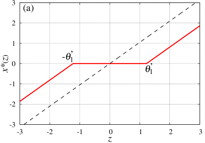
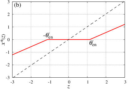
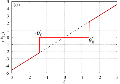
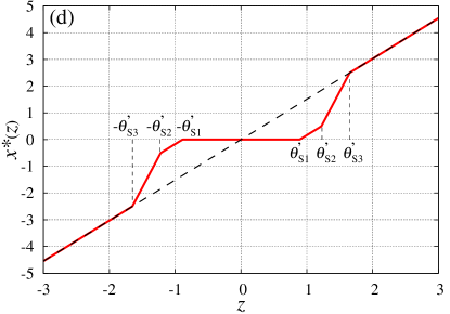
Figure 1: Behaviour of the maximizers of the single-body problem at $\alpha=1$ for (a) $\ell_{1}$ ($\eta=1$), (b) elastic net ($\eta_{1}=1,~{}\eta_{2}=0.5$), (c) $\ell_{0}$ ($\eta=1$), and (d) SCAD regularization ($\eta=1,~{}a=5,~{}\lambda=0.5$). The dashed diagonal lines of gradient 1 are the maximizers under no regularization, and the threshold $\theta^{\prime}$ denotes $\sqrt{2}\theta$.

5.1 $\ell_{1}$ regularization

In the $\ell_{1}$ regularization $r(\bm{x};\eta)=\eta||\bm{x}||_{1}=\eta\sum_{i}|x_{i}|$, the maximizer of the single-body problem (39) is given by

$$x^{*}_{\ell_{1}}(z;\hat{Q},\hat{\chi})=\left\{\begin{array}[]{ll}(h^{\rm RS}(z;\hat{\chi})-\eta{\rm sgn}(z))/\hat{Q}&(|h^{\rm RS}(z;\hat{\chi})|>\eta)\\ 0&({\rm otherwise})\end{array}\right.,$$ (54)

where ${\rm sgn}(z)$ denotes the sign of $z$ and is $0$ when $z=0$. Figure 1 (a) shows the behaviour of $x^{*}_{\ell_{1}}$ at $\alpha=1$ and $\eta=1$. Setting $\theta_{1}=\eta/\sqrt{2\hat{\chi}}$, the fraction of non-zero components is given by the probability that the solution of the RS single-body problem (54) is non-zero: $\hat{\rho}={\rm erfc}(\theta_{1})$, where

$${\rm erfc}(a)=\frac{2}{\sqrt{\pi}}\int_{a}^{\infty}dze^{-z^{2}},$$ (55)

and

$$\pi_{\ell_{1}}=\frac{\hat{\chi}}{\hat{Q}}\Big{\{}(1+2\theta_{1}^{2})\hat{\rho}-\frac{2\theta_{1}}{\sqrt{\pi}}e^{-\theta_{1}^{2}}\Big{\}}.$$ (56)

The regularization-dependent saddle point equations are given by

$$\chi =\frac{\hat{\rho}}{\alpha\hat{Q}}$$ (57)

$$Q =\frac{\hat{\chi}\hat{\tau}_{1}}{\alpha\hat{Q}^{2}},$$ (58)

where

$$\hat{\tau}_{1}=(1+2\theta_{1}^{2})\hat{\rho}-\frac{2\theta_{1}}{\sqrt{\pi}}e^{-\theta_{1}^{2}}.$$ (59)

From (43) and (44), the solutions of the saddle point equations (57) and (58) can be derived as

$$\chi =\frac{\hat{\rho}}{\alpha-\hat{\rho}}$$ (60)

$$Q =\frac{(m_{y}^{2}+\sigma_{y}^{2})\hat{\tau}_{1}}{\alpha-\hat{\tau}_{1}}.$$ (61)

Substituting the saddle point equations, the free energy density and the expectation of the regularization term are given by

$$f =\frac{\alpha\hat{\chi}}{2}+\alpha(\chi\hat{\chi}-Q\hat{Q})$$ (62)

$$\overline{r} =\lim_{N\to\infty}\frac{\eta}{N}E_{\bm{y},\bm{A}}[||\hat{\bm{x}}(\bm{y},\bm{A})||_{1}]=\alpha(\chi\hat{\chi}-Q\hat{Q}),$$ (63)

respectively. Hence, the training error is given by

$$\overline{\rm err}_{\rm train}=\hat{\chi}.$$ (64)

AT instability appears when

$$\frac{\hat{\rho}}{\alpha}>1,$$ (65)

which is outside the region of interest for physical parameters. Equation (60) leads to the following expression for the GDF:

$${\rm df}=\frac{\hat{\rho}}{\alpha}=\delta.$$ (66)

This expression is consistent with the result in [19], which verifies the validity of this RS analysis for the derivation of GDF.

5.2 Elastic net regularization

Elastic net regularization, given by

$$r(\bm{x};\eta_{1},\eta_{2})=\eta_{1}||\bm{x}||_{1}+\frac{\eta_{2}}{2}||\bm{x}||_{2}^{2},$$ (67)

was developed to encourage the grouping effect, which is not exhibited by $\ell_{1}$ regularization, and to stabilize the $\ell_{1}$ regularization path [36]. Here, the coefficient $1/2$ is introduced for mathematical convenience, and $\eta_{2}=0$ and $\eta_{1}=0$ correspond to $\ell_{1}$ regularization and $\ell_{2}$ regularization, respectively.

The solution of the effective single-body problem for elastic net regularization is given by

$$x^{*}_{\rm en}(z;\hat{Q},\hat{\chi})=\left\{\begin{array}[]{ll}(h^{\rm RS}(z;\hat{\chi})-\eta_{1}{\rm sgn}(z))/(\hat{Q}+\eta_{2})&(|h^{\rm RS}(z;\hat{\chi})|>\eta_{1})\\ 0&({\rm otherwise})\end{array}\right..$$ (70)

The behaviour of this solution is shown in Fig. 1 (b) for $\alpha=1,~{}\eta_{1}=1$, $\eta_{2}=0.5$, and

$$\pi_{\rm en}=\frac{\hat{\chi}}{\hat{Q}+\eta_{2}}\Big{\{}(1+2\theta_{\rm en}^{2}){\rm erfc}(\theta_{\rm en})-\frac{2\theta_{\rm en}}{\sqrt{\pi}}e^{-\theta_{\rm en}^{2}}\Big{\}},$$ (71)

where $\theta_{\rm en}=\eta_{1}/\sqrt{2\hat{\chi}}$. The fraction of non-zero components is given by $\hat{\rho}={\rm erfc}(\theta_{\rm en})$, and the regularization-dependent saddle point equations are given by

$$Q =\frac{\hat{\chi}}{\alpha(\hat{Q}+\eta_{2})^{2}}\Big{\{}(1+2\theta_{\rm en}^{2})\hat{\rho}-\frac{2\theta_{\rm en}}{\sqrt{\pi}}e^{-\theta_{\rm en}^{2}}\Big{\}}$$ (72)

$$\chi =\frac{\hat{\rho}}{\alpha(\hat{Q}+\eta_{2})}.$$ (73)

At the saddle point, the free energy density and the expectation of the regularization term can be simplified as

$$f =\frac{\alpha\hat{\chi}}{2}+\alpha(\chi\hat{\chi}-Q\hat{Q})-\frac{\alpha\eta_{2}Q}{2}$$ (74)

$$\overline{r} =\lim_{N\to\infty}\frac{1}{N}E_{\bm{y},\bm{A}}\Big{[}\eta_{1}||\bm{\hat{x}}||_{1}+\frac{\eta_{2}}{2}||\bm{\hat{x}}||_{2}\Big{]}$$ (75)

$$=\alpha\{\hat{\chi}\chi-(\hat{Q}+\eta_{2})Q\}+\frac{\alpha\eta_{2}Q}{2},$$

respectively. Hence, the training error is given by

$$\overline{\rm err}_{\rm train}=\hat{\chi}.$$ (76)

AT instability arises when

$$\frac{\hat{\rho}}{\alpha}>\Big{(}\frac{\hat{Q}+\eta_{2}}{\hat{Q}}\Big{)}^{2};$$ (77)

the right-hand side is always greater than $1$ because $\eta_{2}\geq 0$ and $\hat{Q}>0$. Therefore, the RS solution is always stable under symmetry breaking perturbations in the physical parameter region $\alpha>\hat{\rho}$.

From (73), the GDF for elastic net regularization is given by

$${\rm df}=\frac{\hat{\rho}}{\alpha}-\chi\eta_{2}=\frac{\delta\hat{Q}}{\hat{Q}+\eta_{2}},$$ (78)

which reduces to the GDF for $\ell_{1}$ regularization at $\eta_{2}=0$. An unbiased estimator of the GDF for one instance of $\bm{A}$ is derived in [20] as

$$\hat{\rm df}(\bm{A})=\frac{1}{M}{\rm Tr}(\bm{A}_{{\cal A}}(\bm{A}_{{\cal A}}^{\rm T}\bm{A}_{{\cal A}}+\eta_{2}\bm{I}_{|{\cal A}|})^{-1}\bm{A}_{{\cal A}}^{\rm T}),$$ (79)

where ${\cal A}$ is the set of indices of non-zero components, and the columns $\{\bm{A}_{i}|i\in{\cal A}\}$ constitute the submatrix $\bm{A}_{\cal A}$. The number of the components of ${\cal A}$ is denoted by $|{\cal A}|$. Our expression (78) for df corresponds to the typical value (or the expectation) of $\hat{\rm df}(\bm{A})$ for a Gaussian random matrix $\bm{A}$. The physical implications suggested by the cavity method [32, 38], which is complementary to the replica method, supports the correspondence relationship between $\hat{Q}$ in the replica method and the Gram matrix of $\bm{A}$. This correspondence indicates that our RS analysis is valid for the derivation of GDF under elastic net regularization.

As shown in (78), the GDF for elastic net regularization deviates from $\delta=\hat{\rho}/\alpha$. The $\ell_{2}$ regularization term in elastic net regularization changes the variance of the non-zero components from $\hat{Q}^{-1}$ to $(\hat{Q}+\eta_{2})^{-1}$. Hence, the effective fraction of the non-zero components measured by $\chi/\hat{Q}^{-1}$ does not coincide with $\delta$. By defining the rescaled estimates of the single-body problem as $x^{*{\rm res}}_{\rm en}=(1+\eta_{2}/\hat{Q})x^{*}_{\rm en}$, the corresponding variance is reduced to $\chi^{\rm res}=\hat{\rho}/(\alpha\hat{Q})$ from (47), and this gives ${\rm df}=\delta$. This rescaling corresponds to that shown in [36], which was introduced to cancel out the shrinkage caused by $\ell_{2}$ regularization and improve the prediction performance.

Taking the limit as $\eta_{1}\to 0$, the GDF for $\ell_{2}$ regularization can be obtained where the estimate is not sparse. The solution of the effective single-body problem is given by

$$x^{*}_{\ell_{2}}(z;\hat{Q},\hat{\chi})=\frac{h^{\rm RS}(z;\hat{\chi})}{\hat{Q}+\eta_{2}},$$ (80)

and the function $\pi$ is given by

$$\pi_{\ell_{2}}=\frac{\hat{\chi}}{\hat{Q}+\eta_{2}}.$$ (81)

This expression leads to the following GDF:

$${\rm df}=\frac{\hat{Q}}{\hat{Q}+\eta_{2}},$$ (82)

which corresponds to the limit as $\delta\to 1$ of the elastic net regularization. An unbiased estimator of the GDF for one instance of $\bm{A}$ is proposed as [29]

$$\hat{\rm df}(\bm{A})=\frac{1}{M}{\rm Tr}\bm{A}(\bm{A}^{\rm T}\bm{A}+\eta_{2}\bm{I}_{N})^{-1}\bm{A}^{\rm T}.$$ (83)

Equation (82) corresponds to the expectation of $\hat{\rm df}(\bm{A})$ for a Gaussian random matrix $\bm{A}$.

5.3 $\ell_{0}$ regularization

The $\ell_{0}$ regularization is expressed by $r(\bm{x};\eta)=\eta||\bm{x}||_{0}=\eta\sum_{i}|x_{i}|_{0}$, which corresponds to the number of non-zero components in $\bm{x}$. The solution to the single-body problem for $\ell_{0}$ regularization is given by

$$x_{\ell_{0}}^{*}(z;\hat{Q},\hat{\chi})=\left\{\begin{array}[]{ll}h^{\rm RS}(z;\hat{\chi})/\hat{Q}&(|h^{\rm RS}(z;\hat{\chi})|>\sqrt{2\hat{\chi}}\theta_{0})\\ 0&({\rm otherwise})\end{array}\right.,$$ (86)

where $\theta_{0}=\sqrt{\eta\hat{Q}/\hat{\chi}}$, and by setting the fraction of non-zero components to $\hat{\rho}={\rm erfc}(\theta_{0})$, we can derive

$$\pi_{\ell_{0}}=\frac{\hat{\chi}}{\hat{Q}}\Big{\{}\frac{2\theta_{0}}{\sqrt{\pi}}e^{-\theta_{0}^{2}}+(1-2\theta_{0}^{2})\hat{\rho}\Big{\}}.$$ (87)

Figure 1 (c) shows the $z$-dependence of the maximizer $x^{*}_{\ell_{0}}$ at $\alpha=1$ and $\eta=1$. The regularization-dependent saddle point equations (41)–(42) are given by

$$\chi =\frac{1}{\alpha\hat{Q}}\Big{\{}\frac{2\theta_{0}}{\sqrt{\pi}}e^{-\theta_{0}^{2}}+\hat{\rho}\Big{\}}$$ (88)

$$Q =\frac{\hat{\chi}}{\alpha\hat{Q}^{2}}\Big{\{}\frac{2\theta_{0}}{\sqrt{\pi}}e^{-\theta_{0}^{2}}+\hat{\rho}\Big{\}},$$ (89)

and have two solutions: finite $\chi$ and $Q$ and infinite $\chi$ and $Q$. We denote the finite and infinite solutions as ${\rm S}_{1}=\{\chi_{1},Q_{1}\}$ and ${\rm S}_{2}=\{\chi_{2}=\infty,Q_{2}=\infty\}$, respectively. Using (43) and (44), the finite solution can be simplified as

$$\chi_{1} =\frac{\hat{\rho}+\omega}{\alpha-(\hat{\rho}+\omega)}$$ (90)

$$Q_{1} =(m_{y}^{2}+\sigma_{y}^{2})\chi_{1},$$ (91)

where

$$\omega=\int Dz|z|\delta(|z|-\sqrt{2}\theta_{0})=\frac{2\theta_{0}}{\sqrt{\pi}}e^{-\theta_{0}^{2}}.$$ (92)

By definition, $\chi_{1}$ and $Q_{1}$ should be positive, and so (90)–(91) are only valid when $\alpha>\hat{\rho}+\omega$. According to a local stability analysis of (88) around $1/\chi=0$, solution ${\rm S}_{2}$ is a locally stable solution of the RS saddle point equation when $\alpha<\hat{\rho}+\omega$, where as it is unstable when $\alpha>\hat{\rho}+\omega$. Therefore, the stable solution of the RS saddle point equation changes from ${\rm S}_{1}$ to ${\rm S}_{2}$ at $\alpha=\hat{\rho}+\omega$. Note that the stability discussed here refers to the RS solution, and does not relate to AT instability.

The free energy density is simplified by substituting the saddle point equations as

$$f=\frac{\alpha\hat{\chi}}{2}+\eta\hat{\rho}.$$ (93)

The second term of (93) corresponds to the expectation of the regularization term, and so the training error can be derived as

$$\overline{\rm err}_{\rm train}=\hat{\chi}.$$ (94)

The GDF is given by

$${\rm df}=\left\{\begin{array}[]{ll}\delta+\displaystyle\frac{\omega}{\alpha}&{\rm for~{}solution}~{}{\rm S}_{1}\\ 1&{\rm for~{}solution}~{}{\rm S}_{2}\end{array}\right..$$ (97)

The term $\omega$, given by (92), in the GDF originates from the discontinuity of the single-body problem at the threshold $\sqrt{2}\theta_{0}$, as shown in figure 1 (c). In addition to the fluctuation generated by the non-zero components, this discontinuity induces fluctuations in the system and increases the GDF from $\delta$.

Under $\ell_{0}$ regularization, AT instability always appears, but the estimated GDF under the RS assumption can be regarded as an approximation of the true value of the GDF, as shown in Sec. 8. Our calculations based on the one-step RSB assumption indicate that the form of the GDF, as the fraction of non-zero components plus the discontinuity term, is unchanged, although the values of these two terms does change (unreported).

5.4 SCAD regularization

SCAD regularization is a non-convex sparse regularization in which the estimator has the desirable properties of being unbiased, sparse, and continuous [10]. Mathematically, the SCAD estimator is asymptotically equivalent to the oracle estimator [10, 11]. SCAD regularization is given by

$$r(x;\eta)=\left\{\begin{array}[]{ll}\eta\lambda|x|&(|x|\leq\lambda)\\ -\eta\Big{\{}\displaystyle\frac{x^{2}-2a\lambda|x|+\lambda^{2}}{2(a-1)}\Big{\}}&(\lambda<|x|\leq a\lambda)\\ \displaystyle\frac{\eta(a+1)\lambda^{2}}{2}&|x|>a\lambda\end{array}\right.,$$ (101)

where $\lambda$ and $a$ are parameters that control the form of the regularization. The maximizer of the single-body problem for SCAD regularization is given by

$$x^{*}_{\rm S}(z;\hat{Q},\hat{\chi})=\left\{\begin{array}[]{ll}\displaystyle\frac{h^{\rm RS}(z;\hat{\chi})-\lambda\eta{\rm sgn}(z)}{\hat{Q}}&(\lambda\eta<|h^{\rm RS}(z;\hat{\chi})|\leq\lambda(\hat{Q}+\eta))\\ \displaystyle\frac{h^{\rm RS}(z;\hat{\chi})(a-1)-{a\lambda\eta{\rm sgn}(z)}}{\hat{Q}(a-1)-\eta}&(\lambda(\hat{Q}+\eta)<|h^{\rm RS}(z;\hat{\chi})|\leq a\lambda\hat{Q})\\ \displaystyle\frac{{h}^{\rm RS}(z;\hat{\chi})}{\hat{Q}}&(|h^{\rm RS}(z;\hat{\chi})|>a\lambda\hat{Q})\\ 0&({\rm otherwise})\end{array}\right..$$ (106)

(107)

Figure 1 (d) shows an example of the behaviour of the maximizer $x^{*}_{\rm S}$ at $a=5,\lambda=0.1$, and $\eta=1$, where three thresholds are given by $\theta_{S1}=\lambda\eta/\sqrt{2\hat{\chi}}$, $\theta_{S2}=\lambda(\hat{Q}+\eta)/\sqrt{2\hat{\chi}}$, and $\theta_{S3}=a\lambda\hat{Q}/\sqrt{2\hat{\chi}}$. The threshold $\theta_{{\rm S}1}$ gives the fraction of non-zero components as $\hat{\rho}={\rm erfc}(\theta_{S1})$. Between the thresholds $\theta_{{\rm S}1}$ and $\theta_{{\rm S}2}$, and beyond the third threshold $\theta_{{\rm S}3}$, the estimate $x^{*}_{\rm S}$ behaves like the $\ell_{1}$ and $\ell_{0}$ estimates, respectively. Between $\theta_{{\rm S}2}$ and $\theta_{{\rm S}3}$, the estimate transits linearly between the $\ell_{1}$ and $\ell_{0}$ estimates.

The function $\pi$ for SCAD regularization is derived as

$$\pi_{\rm S}=\pi_{1}+\pi_{2}+\pi_{3}+\frac{\eta\lambda^{2}\pi_{4}}{a-1}-\eta(a+1)\lambda^{2}{\rm erfc(\theta_{{\rm S}3})},$$ (108)

where

$$\pi_{1} \!=\!\frac{\hat{\chi}}{\hat{Q}}\Big{[}\!-\!\frac{2\theta_{S1}}{\sqrt{\pi}}\Big{(}\!e^{-\theta_{S1}^{2}}\!+\!(\frac{\hat{Q}\!-\!\eta}{\eta})e^{-\theta_{S2}^{2}}\!\Big{)}\!+\!(1\!+\!2\theta_{S1}^{2})\{\hat{\rho}\!-\!{\rm erfc}(\theta_{S2}\!)\}\!\Big{]}$$ (109)

$$\pi_{2} =\frac{\hat{\chi}}{\hat{Q}-\frac{\eta}{a-1}}\Big{[}\frac{2}{\sqrt{\pi}}\Big{\{}\Big{(}\theta_{S2}-\frac{2\theta_{S3}\eta}{\hat{Q}(a-1)}\Big{)}e^{-\theta_{S2}^{2}}-\Big{(}1-\frac{2\eta}{\hat{Q}(a-1)}\Big{)}\theta_{S3}e^{-\theta_{S3}^{2}}\Big{\}}$$ (110)

$$+\Big{\{}1+2\Big{(}\frac{\eta\theta_{S3}}{\hat{Q}(a-1)}\Big{)}^{2}\Big{\}}\pi_{4}\Big{]}$$

$$\pi_{3} =\frac{\hat{\chi}}{\hat{Q}}\Big{[}\frac{2\theta_{S3}}{\sqrt{\pi}}e^{-\theta_{S3}^{2}}+{\rm erfc}(\theta_{S3})\Big{]}$$ (111)

$$\pi_{4} ={\rm erfc}(\theta_{S2})-{\rm erfc}(\theta_{S3}).$$ (112)

The regularization-dependent saddle point equations are given by

$$Q =\frac{1}{\alpha}\left\{\frac{\pi_{1}}{\hat{Q}}+\frac{\pi_{2}}{\hat{Q}-\frac{\eta}{a-1}}+\frac{\pi_{3}}{\hat{Q}}\right\}$$ (113)

$$\chi =\frac{1}{\alpha\hat{Q}}\Big{[}\hat{\rho}+\frac{\frac{\eta}{a-1}}{\hat{Q}-\frac{\eta}{a-1}}\pi_{4}\Big{]},$$ (114)

and the expectation of the regularization term is given by

$$\overline{r} =\alpha\chi\hat{\chi}-\pi_{1}-\Big{\{}1+\frac{\frac{\eta}{a-1}}{2(\hat{Q}-\frac{\eta}{a-1})}\Big{\}}\pi_{2}-\pi_{3}-\frac{\eta\lambda^{2}}{2(a-1)}\pi_{4}+\frac{\eta(a+1)\lambda^{2}}{2}{\rm erfc}(\theta_{{\rm S}3}).$$

Substituting these equations into the free energy density, we get

$$\overline{\rm err}_{\rm train}=\hat{\chi}.$$ (116)

The AT instability condition is given by

$$\frac{1}{\alpha(1+\chi)^{2}}\Big{[}\frac{\hat{\rho}}{\hat{Q}^{2}}+\left\{\left(\hat{Q}\!-\!\frac{\eta}{a-1}\right)^{-2}\!\!\!\!\!-\frac{1}{\hat{Q}^{2}}\right\}\pi_{4}\Big{]}>1,$$ (117)

which reduces to that for $\ell_{1}$ regularization as $a\to\infty$.

There are three solutions of $\{Q,\chi\}$: ${\rm S}_{1}=\{Q=Q_{1}<\infty,\chi=\chi_{1}<\infty\}$, ${\rm S}_{2}=\{Q=Q_{2}<\infty,\chi=\infty\}$, and ${\rm S}_{3}=\{Q=\infty,\chi=\infty\}$. For sufficiently large $a$, the finite solution ${\rm S}_{1}$ is a locally stable solution of the RS saddle point equation when

$$\alpha>\hat{\rho}+\frac{\eta/\{\hat{Q}(a-1)\}}{1-\eta/\{\hat{Q}(a-1)\}}\pi_{4}.$$ (118)

Beyond the range of (118), the stable RS solution is replaced by ${\rm S}_{2}$. For sufficiently small $\eta$, the stable RS solution can switch from ${\rm S}_{2}$ to ${\rm S}_{3}$ depending on the SCAD parameter, but this is not important in estimating the GDF, because both solutions give the same GDF value. The GDF for SCAD regularization can be summarized as

$${\rm df}=\left\{\begin{array}[]{ll}\delta+\displaystyle\frac{\frac{\eta}{a-1}}{\alpha(\hat{Q}-\frac{\eta}{a-1})}\pi_{4}&{\rm for~{}solution~{}S}_{1}\\ 1&{\rm for~{}solutions~{}S}_{2}{\rm~{}and~{}S}_{3}\end{array}\right..$$ (121)

As $a\to\infty$, we get $\pi_{4}\to 0$ and solution ${\rm S}_{1}$ is always a stable RS solution, satisfying (118); hence, the GDF reduces to that for $\ell_{1}$ regularization. The second term of the GDF for solution ${\rm S}_{1}$ arises from the weight between the thresholds $\theta_{{\rm S}2}$ and $\theta_{{\rm S}3}$. The manner of assigning the non-zero components to this transient region between the $\ell_{1}$ and $\ell_{0}$ estimates increases the fluctuation in the system, and the GDF does not coincide with $\delta$.

We note the pathology of solution ${\rm S}_{3}$ under the RS assumption. As shown in the solution to the single-body problem (107) (Fig. 1 (d)), the magnitude relation $\theta_{{\rm S}1}\leq\theta_{{\rm S}2}\leq\theta_{{\rm S}3}$ should hold. However, the $Q,\chi\to\infty$ solution leads to $\theta_{{\rm S}3}\to 0$ with finite $\theta_{{\rm S}1}=\theta_{{\rm S}2}$. Solution ${\rm S}_{3}$ appears in the region where AT instability appears, and so this non-physical phenomenon is considered to be caused by an inappropriate RS assumption. Hence, we must construct the RSB solution to correctly describe the GDF corresponding to solution ${\rm S}_{3}$.

6 Parameter dependence of GDF and prediction error

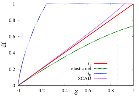
Figure 2: $\delta$-dependence of GDF for $\ell_{1}$, elastic net, $\ell_{0}$, and SCAD regularization at $\alpha=0.5$, $m_{y}=0$, and $\sigma_{y}^{2}=1$. The parameters for elastic net and SCAD regularization are $\eta_{2}=0.1$, $a=8$, and $\lambda=1$, and the vertical dashed line indicates the appearance of the AT instability for SCAD regularization, $\delta=0.866$. The $\ell_{1}$ result corresponds to the line ${\rm df}=\delta$.

Figure 2 illustrates the $\delta$-dependence of the GDF for $\ell_{1}$, the elastic net with $\eta_{2}=0.1$, $\ell_{0}$, and SCAD regularization with $a=8$ and $\lambda=1$ at $\alpha=0.5$, $m_{y}=0$, and $\sigma_{y}^{2}=1$. At each point of $\delta$, the regularization parameters $\eta$ for $\ell_{1}$, $\ell_{0}$ and SCAD regularization and $\eta_{2}$ for elastic net regularization are controlled such that $\delta=\hat{\rho}/\alpha$. Under $\ell_{1}$ regularization, the GDF is always equal to $\delta$, as shown in (66). In elastic net regularization, the GDF is less than $\delta$ as the $\ell_{2}$ parameter $\eta_{2}$ increases. For $\ell_{0}$ regularization, the RS solution ${\rm S}_{1}$ is unstable at $\delta>0.248$ in this parameter region, and is replaced by solution ${\rm S}_{2}$, which gives ${\rm df}=1$. In SCAD regularization, the solution ${\rm S}_{1}$ loses local stability within the RS assumption at $\delta>0.924$, and AT instability appears before the RS solution ${\rm S}_{1}$ becomes unstable at $\delta>0.866$ (denoted by the dashed vertical line in figure 2.)

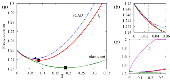
Figure 3: (a) $\delta$-dependence of the prediction error $\overline{\rm err}_{\rm pre}$ for $\ell_{1}$, elastic net, and SCAD regularization at $\alpha=0.5$, $m_{y}=0.5$, and $\sigma_{y}^{2}=1$. The parameters for elastic net and SCAD regularization are $\eta_{2}=0.1$, $a=8$, and $\lambda=1$. (b) Region where the magnitude relationship between each regularization changes. (c) Prediction error for $\ell_{0}$ regularization.

Figure 3 shows the prediction error (26) for the same parameter region as figure 2. At $\sigma_{y}^{2}=1$, the prediction error is equivalent to the expectation of AIC. In the entire range of $\delta$ shown in figure 3 (a), the RS solutions for $\ell_{1}$, elastic net, and SCAD regularization are stable under symmetry breaking perturbations. Thus, we can identify the value of $\delta$ that minimizes the prediction error for each regularization. In this case, the models with $\delta=0.085$ (denoted by •), $\delta=0.170$ ($\blacksquare$), and $\delta=0.072$ ($\blacktriangle$) are selected for $\ell_{1}$, elastic net, and SCAD regularization, respectively. In the current problem setting, sparse estimation with SCAD regularization minimizes the prediction error within the RS region when the mean of the data is sufficiently small. To identify the appropriate model using RS analysis, it is useful to standardize the data. As shown in figure 3 (b), the magnitude of the prediction errors at $\delta<\delta_{1}=0.028$, $\delta_{1}<\delta<\delta_{2}=0.045$, and $\delta>\delta_{2}$ runs in descending order as elastic net$>$SCAD$>\ell_{1}$, SCAD$>$elastic net$>\ell_{1}$, and SCAD$>\ell_{1}>$elastic net, respectively. The estimates $\hat{\bm{x}}$ have different supports depending on the regularization, even when the regularization parameters are controlled to give a certain value of $\delta$. A comparison of the prediction errors within the framework of RS analysis guides the choice of regularization for each value of $\delta$.

The prediction error for $\ell_{0}$ regularization under the RS assumption is shown in figure 3 (c) alongside those for other regularization types. The RS prediction error is minimized at $\delta=0$. This indicates that the appropriate model under RS analysis has a non-zero component of $O(1)$. Our analysis assumes that the number of non-zero components is $O(N)$; hence, the derived model selection criterion cannot identify the appropriate model in the current problem setting for $\ell_{0}$ regularization.

7 Numerical calculation of GDF using belief propagation algorithm

7.1 Belief propagation algorithm for sparse regularization

The correspondence between replica analysis and the belief propagation (BP) algorithm suggests that the typical properties of BP fixed points at the large-system-size limit can be described by the RS saddle point [32, 38]. Thus, we may expect that the numerically obtained GDF will be consistent with the RS analysis at finite system sizes using the BP algorithm. For the ordinary least squares with a regularization that can be written as (12), a tentative estimate of the $i$-th component at step $t$, denoted by $\hat{x}_{i}^{(t)}$, is given by the solution to the single-body problem (39) with the substitutions $\hat{Q}\to\hat{Q}_{i}^{(t)}$ and $h^{\rm RS}(z;\hat{\chi})\to h_{i}^{(t)}$ [25, 26, 27], where

$$h_{i}^{(t)} =\hat{x}_{i}^{(t-1)}\sum_{\mu=1}^{M}\frac{A_{\mu i}^{2}}{1+{\sigma_{\mu}^{(t-1)}}^{2}}+\sum_{\mu=1}^{M}A_{\mu i}R_{\mu}^{(t-1)}$$ (122)

$$\hat{Q}_{i}^{(t)} =\sum_{\mu=1}^{M}\frac{A_{\mu i}^{2}}{1+{\sigma_{\mu}^{(t-1)}}^{2}},$$ (123)

and setting $\hat{\bm{y}}^{(t)}=\bm{A}\hat{\bm{x}}^{(t)}$,

$$R_{\mu}^{(t)} =\frac{y_{\mu}-\hat{y}_{\mu}^{(t)}}{1+{\sigma_{\mu}^{(t)}}^{2}}$$ (124)

$${\sigma_{\mu}^{(t)}}^{2} =\frac{1}{\alpha}\sum_{i}A_{\mu i}^{2}\chi_{i}^{(t)}.$$ (125)

The variable $\chi_{i}^{(t)}$ represents the variance of $x_{i}^{(t)}$, and its determination rule depends on the regularization. For $\ell_{1}$ and elastic net regularization, the variable is given by

$$\chi_{i}^{(t)}=\left\{\begin{array}[]{ll}\displaystyle\frac{1}{\hat{Q}_{i}^{(t)}}&{\rm for}~{}|h_{i}^{(t)}|>\eta\\ 0&{\rm otherwise}\end{array}\right.$$ (128)

and

$$\chi_{i}^{(t)}=\left\{\begin{array}[]{ll}\displaystyle\frac{1}{\hat{Q}_{i}^{(t)}+\eta_{2}}&{\rm for}~{}|h_{i}^{(t)}|>\eta_{1}\\ 0&{\rm otherwise}\end{array}\right.,$$ (131)

respectively. For these regularizations, the GDF at the BP fixed point converges to that given by RS analysis as the system size increases. However, for these regularizations, the GDF can be calculated using least angle regression (LARS) [37], which has a lower computational cost than the BP algorithm. Hence, there is no need to introduce the BP algorithm. In the case of $\ell_{0}$ regularization, the variable $\chi_{i}$ is given by

$$\chi_{i}^{(t)}=\left\{\begin{array}[]{ll}\displaystyle\frac{1}{\hat{Q}_{i}^{(t)}}&{\rm for}~{}|h_{i}^{(t)}|>\sqrt{2\eta\hat{Q}_{i}^{(t)}}\\ 0&{\rm otherwise}\end{array}\right..$$ (134)

Unfortunately, AT instability appears across the whole parameter region for $\ell_{0}$ regularization, and the BP algorithm does not converge.

For SCAD regularization, no numerical method for the precise evaluation of GDF has been proposed. As shown in the previous section, SCAD regularization gives a parameter region where the RS solution is stable. Therefore, the BP algorithm is useful as a method of numerically calculating the GDF for SCAD regularization. The variable ${\chi}_{i}^{(t)}$ for SCAD regularization is given by

$${\chi_{i}^{(t)}} =\left\{\begin{array}[]{ll}\displaystyle\frac{1}{\hat{Q}_{i}^{(t)}}&{\rm for~{}}\lambda\eta<|h^{(t)}_{i}|\leq\lambda(\hat{Q}_{i}^{(t)}+\eta)\mbox{ and }|h^{(t)}_{i}|>a\lambda\hat{Q}^{(t)}_{i}\\ \displaystyle\frac{1}{\hat{Q}_{i}^{(t)}-\frac{\eta}{a-1}}&\mbox{for }\lambda(\hat{Q}_{i}^{(t)}+\eta)<|h_{i}^{(t)}|\leq a\lambda\hat{Q}_{i}^{(t)}\\ 0&{\rm otherwise}\end{array}\right..$$ (138)

After updating the estimates $\hat{\bm{x}}^{(t)}$, we can numerically evaluate the value of GDF using (8) with the data estimates $\hat{\bm{y}}^{(t)}$. To ensure convergence, appropriate damping is required at each update.

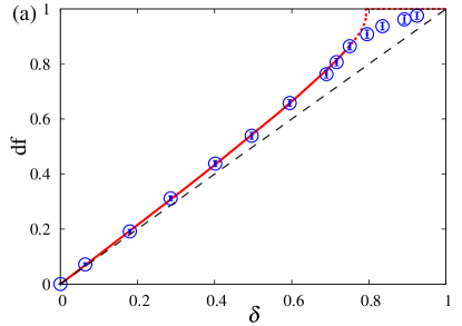
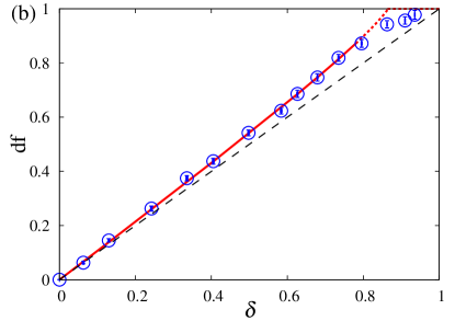
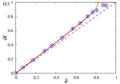
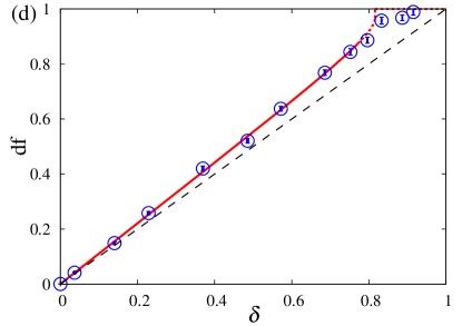
Figure 4: Comparison between BP algorithm and RS analysis for SCAD regularization at $N=200$, $m_{y}=0$, and $\sigma_{y}^{2}=1$ for (a) $a=5$, $\lambda=1$ for $M=100$ ($\alpha=0.5$), (b) $a=8$, $\lambda=0.8$ for $M=100$ ($\alpha=0.5$), (c) $a=6$, $\lambda=0.9$ for $M=160$ ($\alpha=0.8$), and (d) $a=8$, $\lambda=0.7$ for $M=160$ ($\alpha=0.8$). The BP results, averaged over 100 realizations of $\{\bm{y},\bm{A}\}$, are denoted by circles. The theoretical estimation of GDF by RS analysis is denoted by solid and dashed lines for the RS and RSB regions, respectively. To provide a visual guide, the dashed line has a gradient of $1$.

As for the replica analysis, we apply the BP algorithm for the case of Gaussian random data $\bm{y}$ and predictors $\bm{A}$. Figure 4 shows the numerically calculated GDF given by the BP algorithm at $N=200$, $m_{y}=0$, and $\sigma_{y}^{2}=1$. The BP algorithm is updated until $|\hat{x}_{i}^{(t)}-\hat{x}_{i}^{(t-1)}|<10^{-10}$ for each component, and the result is averaged over 100 realizations of $\{\bm{y},\bm{A}\}$. The solid and dashed lines represent the analytical results given by the replica method for the RS and RSB regions, respectively. In the RS regime, the numerically calculated GDF from the BP algorithm coincides with that evaluated by the replica method.

7.2 Perspective for other predictors

The RS analysis discussed so far has been applied to Gaussian i.i.d. random predictors. Its extension to other predictors is not straightforward. To check the generality of the GDF being given by the effective fraction of non-zero components $(\chi/\hat{Q}^{-1})$ at the RS saddle point for other predictor matrices, we resort to the BP algorithm. The typical properties of $\chi_{i}^{(t)}$ and $\hat{Q}_{i}^{(t)}$ at the BP fixed point denoted by $\chi_{i}^{*}$ and $\hat{Q}_{i}^{*}$ are described in the replica method by $\chi$ and $\hat{Q}$ of the RS saddle point at the large-system-size limit. Therefore, it is reasonable to define the effective fraction of non-zero components at the BP fixed point as

$$\delta^{\rm BP}_{\rm eff}=\frac{\overline{\frac{1}{N}\sum_{i}\chi_{i}^{*}(\bm{y},\bm{A})}}{\left(\overline{\frac{1}{N}\sum_{i}\hat{Q}^{*}_{i}(\bm{y},\bm{A})}\right)^{-1}},$$ (139)

where the overline represents the average over $\bm{y}$ and $\bm{A}$. If $\delta_{\rm eff}^{\rm BP}$ and the GDF from (8) coincide at the BP fixed point, it is considered that the correspondence between GDF and the effective fraction of non-zero components holds at the RS saddle point. For $\ell_{1}$, elastic net, and SCAD regularization, we examine the behaviour of GDF and $\delta_{\rm eff}^{\rm BP}$ under two predictors [36] in a parameter region where the BP algorithm converges.

Example 1:

Gaussian predictors with pairwise correlation. The correlation between predictors $\bm{A}_{i}$ and $\bm{A}_{j}$ is set to be $c^{|i-j|}$, and the predictors are normalized such that $||\bm{A}_{i}||_{2}^{2}=1$.

Example 2:

The predictors are generated as

$$\bm{A}_{i}=\left\{\begin{array}[]{ll}\bm{Z}_{1}+\bm{\epsilon}_{i}&{\rm for}~{}i=1,\cdots,T\\ \bm{Z}_{2}+\bm{\epsilon}_{i}&{\rm for}~{}i=K+1,\cdots,2T\\ \bm{Z}_{3}+\bm{\epsilon}_{i}&{\rm for}~{}i=2K+1,\cdots,3T\\ \bm{a}_{i}&{\rm for}~{}i=3T+1,\cdots,N\\ \end{array}\right.,$$ (144)

where the components of the $M$-dimensional vectors $\bm{Z}_{1},\bm{Z}_{2},\bm{Z}_{3}$, $\{\bm{a}_{i}\}$, and $\{\bm{\epsilon}_{i}\}$ are i.i.d. Gaussian random variables with mean zero and variance $1$, and $T$ is a parameter that takes an integer value smaller than $(N-1)/3$. The predictors are normalized such that $||\bm{A}_{i}||_{2}^{2}=1$.

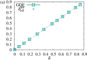
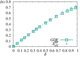
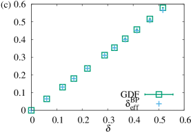
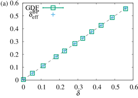
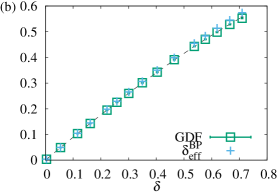
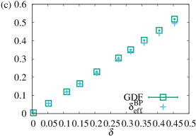
Figure 5: $\delta$-dependence of GDF and $\delta_{\rm eff}^{\rm BP}$ at BP fixed point of $N=1000$, $M=500$ $(\alpha=0.5)$ for (a) $\ell_{1}$, (b) elastic net of $\eta_{2}=0.1$, and (c) SCAD regularization of $a=0.5$ and $\lambda=1$ under the predictor matrix of example 1 with $c=0.5$. We used 1000 samples of predictor matrices to calculate the GDF and $\delta_{\rm eff}^{\rm BP}$ at the BP fixed point. The $\delta$-region where the BP algorithm converges within $10^{5}$ steps is shown. The dashed lines in (a) and (b) denote the results reported in [19] and [20].

Figure 6: $\delta$-dependence of GDF and $\delta_{\rm eff}^{\rm BP}$ at BP fixed point of $N=1000$, $M=500$ $(\alpha=0.5)$ for (a) $\ell_{1}$, (b) elastic net of $\eta_{2}=0.1$, and (c) SCAD regularization of $a=0.5$ and $\lambda=1$ under the predictor matrix of example 2 with $T=125$. We used 1000 samples of predictor matrices to calculate the GDF and $\delta_{\rm eff}^{\rm BP}$ at the BP fixed point. The $\delta$-region where the BP algorithm converges within $10^{5}$ steps is shown. The dashed lines in (a) and (b) denote the results reported in [19] and [20].

Figures 6 and 6 show the $\delta$-dependence of GDF and $\delta_{\rm eff}^{\rm BP}$ at the BP fixed point for $\ell_{1}$, elastic net, and SCAD regularization at $N=1000$ and $\alpha=0.5$ $(M=500)$. The values of each point have been averaged over 1000 samples of $\{\bm{y},\bm{A}\}$. Under $\ell_{1}$ and elastic net regularization, the GDF value calculated as the expectation of the unbiased estimator derived in [19, 20] is shown as a dashed line. In both examples, the correspondence between GDF and $\delta_{\rm eff}^{\rm BP}$ holds for each regularization, although a small discrepancy appears due to finite-size effects at large $\delta$. Furthermore, the values of $\delta_{\rm eff}^{\rm BP}$ and GDF at the BP fixed point are consistent with those of previous studies for $\ell_{1}$ and elastic net regularization. The parameters $c$ and $T$ in these examples do not influence the results, although they do affect the convergence of the BP algorithm. These results imply that the correspondence between GDF and the effective fraction of non-zero components holds outside of Gaussian i.i.d. predictors. For both examples, the convergence of the BP algorithm is worse than with the Gaussian i.i.d. predictors, particularly at large $\delta$. Thus, the algorithm must be improved to enable a discussion of the large-$\delta$ region and application to other predictor matrices.

In the case of $\ell_{0}$ regularization, the BP algorithm does not converge. Thus, we cannot confirm the generality of the result using the properties of BP fixed points. The replica analysis for non-Gaussian i.i.d. predictor matrices is a necessary step towards verifying the generality of the result for $\ell_{0}$ regularization. Although the range of applicable predictor matrices for replica analysis is narrower than that for the BP algorithm, the analysis of rotationally invariant predictor matrices offers a promising means towards demonstrating the generality [21].

8 RS solution approximates the GDF for $\ell_{0}$ regularization

For $\ell_{0}$ regularization, the RS solution is unstable in the whole parameter region, but it is known that this solution generally approximates the true solution. One can numerically obtain the exact solution of (12) for $\ell_{0}$ regularization by an exhaustive search, and calculate the exact value of GDF at small system sizes. Comparing the GDF under RS analysis with its exact value, we can evaluate the approximation performance of the RS solution.

Figure 7 compares the GDF approximated by the RS solution with its exact value for $N=20,30$, and $50$ as calculated by 1000 samples of $\{\bm{y},\bm{A}\}$. As $N$ increases, the exact GDF approaches the RS solution, although intense finite-size effects are observed in the small-$\delta$ region. For a comparison at larger system sizes, we must develop a computationally feasible algorithm for obtaining precise solutions of (12) for $\ell_{0}$ regularization, but this is beyond the scope of the present paper.

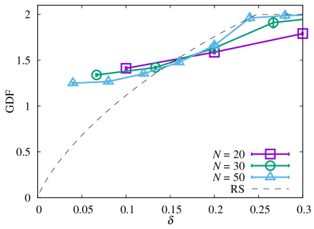
Figure 7: Comparison between exact value of GDF at finite system sizes and GDF under RS analysis.

9 Summary and Conclusion

We have derived the GDF using a method based on statistical physics. Within the range of the RS assumption, the GDF is represented as $\chi/\hat{Q}^{-1}$, where $\chi$ and $\hat{Q}^{-1}$ correspond to the rescaled variance around estimates and the variance of estimates when the regularization term is omitted, respectively. This expression does not depend on the type of regularization, and indicates that GDF can be regarded as the effective fraction of non-zero components.

We applied our method for the derivation of GDF to $\ell_{1}$, elastic net, $\ell_{0}$, and SCAD regularization. Our RS analysis was stable for $\ell_{1}$ and elastic net regularization in the entire physical parameter region, and the GDFs for these regularizations were consistent with previous results. This correspondence supports the validity of our RS analysis. The model selection criterion of prediction error was derived by combining the GDF with the training error. Theoretical predictions in the RS phase were then algorithmically achieved using the belief propagation method.

It has been implied that the equivalence between GDF and the ratio of the number of non-zero components to the number of samples, $\delta$, only holds for $\ell_{1}$ regularization [19]. Our representation of GDF as the effective fraction of non-zero components clarifies the origin of the additional component of the GDF from the fraction of non-zero components.

• In $\ell_{1}$ regularization, the GDF is given by $\delta$ because there is no factor that induces fluctuations other than the non-zero components.

• Elastic net regularization changes the variance of the components, and so the GDF does not coincide with $\delta$. However, as with $\ell_{1}$ regularization, the non-zero components are the unique source of fluctuations, and so the correspondence between GDF and $\delta$ can be recovered by appropriately rescaling the estimates.

• In $\ell_{0}$ regularization, the discontinuity of the estimates leads to additional fluctuations besides those caused by the non-zero components. Hence, the GDF is greater than $\delta$.

• In SCAD regularization, the assignment of non-zero components to the transient region between $\ell_{1}$-type estimates and $\ell_{0}$-type estimates induces additional components in the GDF.

For regularizations with AT instabilities in certain parameter regions (e.g. $\ell_{0}$, SCAD, and other non-convex regularizations), it is generally necessary to construct the full-step RSB solution. In the case of SCAD regularization, model selection based on the prediction error under RS analysis can be achieved in the current problem setting. Even when the RS solution is unstable, the prediction error gives a meaningful approximation of the true value.

Further development of our method for the general function of prediction error [39] and real data will be useful for practical applications. The BP algorithm discussed here can numerically calculate the GDF and model selection criterion for practical settings at reasonable computational cost.

References

References

- [1] Akaike H 1973 Second International Symposium on Information Theory (Petrov B N and Csaki F, eds.) 267 Académiai Kiadó, Budapest.
- [2] Tibshirani R 1996 J. Roy. Statist. Soc. Ser. B 58 267
- [3] Candès E J and Tao T 2005 IEEE Trans. Inform. Theory 51 4203
- [4] Donoho D 2006 IEEE Trans. Inform. Theory 52 1289
- [5] Girolami M 2001 Neural Comput. 13 2517
- [6] Zhu J, Rosset S, Hastie T and Tibshirani R 2004 Adv. Neural. Inf. Process 16 49
- [7] Foucart S and Lai M-J 2009 Appl. Comput. Harmon. Anal. 26 395
- [8] Wang M, Xu W and Tang A 2011 IEEE Trans. Inform. Theory 57 7255
- [9] Xu Z, Chang X, Xu F and Zhang H 2012 IEEE Trans. Neural Networks and Learning Systems 23 1013
- [10] Fan J and Li R 2001 J. Amer. Statist. Assoc. 96 1348
- [11] Fan J and Peng H 2004 Annal. Stat. 32 928
- [12] Huang J, Ma S and Zhang C-H 2008 Statistica Sinica 18 1603
- [13] Stone M 1974 Biometrika 61 509
- [14] Zhang Y, Li R and Tsai C-L 2010 J. Amer. Statist. Assoc. 105 312
- [15] Obuchi T and Kabashima Y arXiv:1601.00881
- [16] Ye J 1998 J. Amer. Statist. Assoc. 93 120
- [17] Mallows C 1973 Technometrics 15 661
- [18] Efron B 2004 J. Amer. Statist. Assoc. 99 619
- [19] Zou H, Hastie T and Tibshirani R 2007 Annal. Stat. 35 2173
- [20] Zou H 2005 Ph.D. dissertation Dept. Statistics, Stanford Univ.
- [21] Kabashima Y, Wadayama T and Tanaka T 2009 \JSTAT L09003
- [22] Rangan S, Goyal V and Fletcher A K 2009 in Y. Bengio et al. (eds.), Advances in Neural Information Processing Systems 22 1545
- [23] Guo D, Baron D and Shamai (Shitz) S 2009 Proceedings of the 47th Annual Allerton Conference on Communication, Control, and Computing 52
- [24] Sakata A and Kabashima Y 2013 Europhys. Lett. 103 28008
- [25] Donoho D L, Maleki A and Montanari A 2009 Proc. Nat. Acad. Sci. USA 106 18914
- [26] Donoho D L, Maleki A and Montanari A 2011 IEEE Trans. Inf. Theory 57 6920
- [27] Rangan S 2011 in Proceedings of the 2011 IEEE International Symposium on Information Theory Proceedings (ISIT), Austin, Texas (IEEE,New York), 2168
- [28] Krzakala F, Mézard M, Sausset F, Sun Y F and Zdeborova L 2012 Phys. Rev. X 2 021005
- [29] Hastie T and Tibshirani R 1990 Generalized Adaptive Models (Chapman and Hall, London)
- [30] Stein C 1981 Annal. Stat. 9 1135
- [31] Donoho D and Johnstone I 1995 J. Amer. Statist. Assoc. 90 1200
- [32] Mézard M, Parisi G and Virasoro M 1987 Spin Glass Theory and Beyond (World Scientific)
- [33] Nishimori H 2001 Statistical Physics of Spin Glasses and Information Processing: An Introduction (Oxford: Oxford University Press)
- [34] Nakanishi-Ohno Y, Obuchi T, Okada M and Kabashima Y arXiv:1510.02189.
- [35] de Almeida J R L and Thouless D J 1978 J. Phys. A: Math. Gen. 11 983
- [36] Zou H and Hastie T 2005 J. R. Statist. Soc. B 67 301
- [37] Efron B, Hastie T, Johnstone I and Tibshirani R 2004 Annal. Stat. 32 407
- [38] Mézard M and Montanari A 2009 Information, Physics, and Computation (Oxford: Oxford Press)
- [39] Efron B 1986 J. Amer. Statist. Assoc. 81 461